Efficiency Gains from the Elimination of Global Restrictio… · In this paper we compute the world-wide efficiency gains from the elimination of restrictions on labour mobility

EFFICIENCY GAINS FROM THE ELIMINATION OF GLOBAL RESTRICTIONS ON

LABOUR MOBILITY:

AN ANALYSIS USING A MULTIREGIONAL CGE MODEL

Ana María IreguiEstudios EconómicosBanco de la República

Bogotá, Colombia

December 1999

ABSTRACT

We compute the world-wide efficiency gains from the elimination of global restrictions on labourmobility using a multiregional CGE model. A distinctive feature of our analysis is the introductionof a segmented labour market, as two types of labour are considered: skilled and unskilled.According to our results, when labour is a homogeneous factor, the elimination of globalrestrictions on labour mobility generates world-wide efficiency gains that could be of considerablemagnitude. When the labour market is segmented and both skilled and unskilled labour migrate,welfare gains reduce since the benefits and losses of migration are not evenly distributed withineach region. When only skilled labour migrates, the world-wide efficiency gains are smaller, sincethis type of labour represents a small fraction of the labour force in developing regions.

Keywords: Migration, applied CGE modelling, labour market segmentation.

JEL classification: C68, F22, R13, R23

* I wish to thank Chris Dawkins, Jesús Otero, Jeff Round, John Whalley and the participants of theXVII Latin American meeting of the Econometric Society for helpful comments and suggestions.The views expressed in the paper are those of the author.

1

1. INTRODUCTION

The classic economic argument in favour of labour migration is that people move in search of

higher wages, hence increasing their own productivity. 1 However, as indicated by Layard et al.

(1992), the decision to migrate also depends upon other economic, social and political

considerations. Among the economic aspects, migrants may take into account comparative wage

levels (actual and expected); comparative unemployment rates and unemployment benefits; the

availability of housing; and the cost of migration which includes travel expenses, information costs,

and the psychological cost of leaving friends and family. Weyerbrock (1995) also indicates that

political instability and civil war may cause larger emigration flows than economic or demographic

pressures.

Recent empirical studies on international migration have mainly focused on U.S.-Mexico

migration patterns (Hill and Méndez, 1984, Robinson et al., 1993; Levy and van Wijnbergen, 1994),

and migration flows from Eastern Europe and the former Soviet Union into Western Europe

(Layard et al., 1992; Weyerbrock,1995).

Hamilton and Whalley (1984) has been the only attempt to quantify the efficiency gains

from the removal of global restrictions on labour mobility. They use a partial equilibrium

framework, in which the parameters of a CES production function are estimated for a seven-region

country classification. Then, the estimated parameters are used to calculate the changes in labour

allocation across regions after the removal of immigration controls. They assume that the world-

wide labour supply is fixed, that full employment occurs in all regions, and that differences in

labour’s marginal product across regions arise from barriers to inward mobility of labour in high

wage countries. Hamilton and Whalley find large efficiency gains from the removal of immigration

controls; in most cases, these gains exceed world-wide GNP generated in the presence of the

controls. In addition, in labour exporting regions wage rates rise and capital owners are made worse

1 Layard et al. (1992) indicate that free trade and international capital mobility can also raise productivity,without labour migration.

2

off; on the other hand, in labour receiving regions wage rates fall and capital owners are made better

off.

In this paper we compute the world-wide efficiency gains from the elimination of

restrictions on labour mobility. In contrast to Hamilton and Whalley (1984), we use a multiregional

general equilibrium model instead of a partial equilibrium approach, since the former provides an

ideal framework to analyse the effects of policy changes on resource allocation, the structure of

distribution, and thus in economic welfare. A distinctive feature of our analysis is that we consider a

segmented labour market (i.e., skilled and unskilled labour), which can be justified on the grounds

that this factor is not homogeneous. The segmentation of the labour market jointly with the general

equilibrium framework allow us to examine the distributional effects of migration between skilled

and unskilled labour in each region, and between these two and capital.

According to our results, the elimination of global restrictions on labour mobility generates

world-wide efficiency gains that could be of considerable magnitude, ranging from 15% to 67% of

world GDP. With the introduction of a segmented labour market, welfare gains reduce since the

benefits and losses of migration are not evenly distributed within each country, ranging from 13%

to 59% of world GDP. And when only skilled labour migrates, world-wide efficiency gains are

smaller ranging from 3% to 11% of world GDP, since skilled labour represents a small fraction of

the labour force in developing regions.

The paper proceeds as follows. Section 2 describes the basic structure of our multiregional

general equilibrium model. Section 3 contains the empirical implementation, including the

description of the benchmark data set and the calibration of the model. Section 4 presents the results

of the model as well as the sensitivity analysis. Section 5 presents model elaborations, including

transaction costs, international capital mobility, and selective mobility. Section 6 offers some

concluding remarks.

3

2. THE MODEL

In a world economy characterised by countries with different levels of income, individuals have

incentives to migrate to countries with higher wage rates. If labour were allowed to move from one

country to another without restrictions, it will do so until the marginal product of labour is the same

in both low income and high income countries. Migration will reduce the labour force in the low

income country (source region), leading to an increase in wages,2 and a reduction in the demand for

labour. In addition, migration leads to a process of factor reallocation within the poor country: the

remaining workers gain through higher wages, but capital owners lose since labour is now scarce

relative to capital. Conversely, in the high income country (destination region) the labour force

increases, which leads to a reduction in the wage rate (assuming no rigidities). This lower wage will

increase the demand for labour and aggregate employment. During the transition, workers will lose

through lower wages and capital owners will gain since labour is now less scarce relative to capital

(see e.g. Bhagwati et al., 1998; Layard et al. 1992). This analysis is based on the assumption that

labour is a homogeneous factor of production, which implies that the benefits and loses of migration

are evenly distributed within each country. However, as our analysis will show later on, this is not

necessarily the case when there are many types of labour.3

2 The magnitude of the increase will depend on the elasticity of labour demand. The more elastic the demandfor labour, the smaller the increase in wages.3 For some trade theorists the issue of the removal of restrictions on labour mobility may not be of greatrelevance because of the factor price equalisation theorem, according to which factor prices will be equalisedby free trade without internationally mobile factors (see Samuelson 1948, 1949). However, this theorem isbased on very restrictive assumptions, such as identical technologies in different countries, constant returns toscale, perfect competition, no factor intensity reversals, no specialisation, and that good prices are equalisedas a result of trade. Moreover, factor price equalisation depends on the complete convergence of the price ofthe goods. In reality, the prices of the goods are not fully equalised because of both natural (e.g.,transportation costs) and artificial barriers to trade (e.g., import tariffs, import quotas, voluntary exportrestraints). An additional reason why factor price equalisation may not be achieved is that countries exhibitdifferent technologies and resources, so that they are unlikely to remain unspecialised (see e.g. Layard andWalters 1978, Krugman and Obstfeld 1994).

4

2.1 STRUCTURE OF THE MODEL

The structure of the model follows the standard specification of a multiregional general equilibrium

model. The model is static, and consists of eight regions, each one with demand and production

structures, linked through trade. Each region contains one industry that produces a single output,

which is treated as heterogeneous across regions (Armington, 1969). There is a representative

consumer in each region and, for simplicity, intermediate production is not considered.

On the production side we consider two variants. In the first variant, production involves a

CES value added function with capital (K) and labour (L) as primary inputs; factor demands are

obtained from cost minimisation. In the second variant of the model, we consider capital (K) and

two types of labour: skilled (Ls) and unskilled (Lu). In other words, the labour market is assumed to

be segmented and this, as indicated above, is a distinctive feature of our modelling exercise in

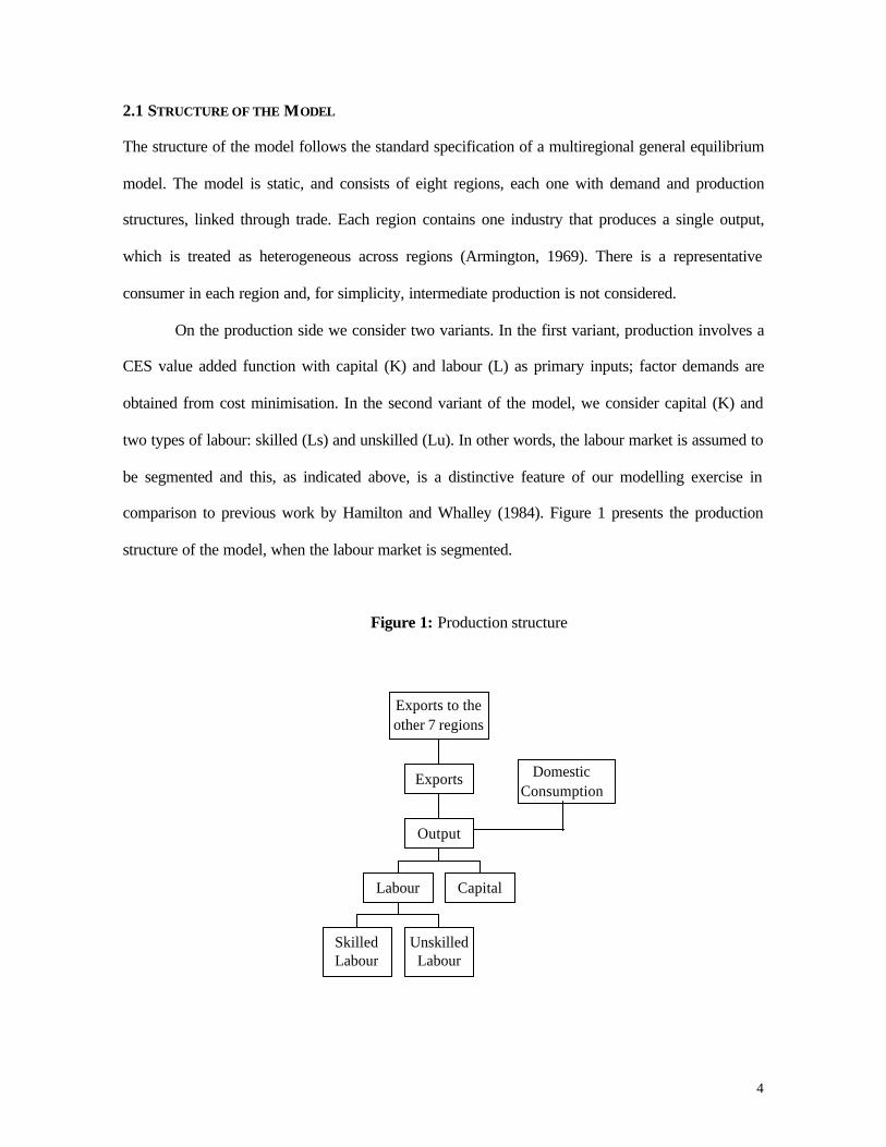
comparison to previous work by Hamilton and Whalley (1984). Figure 1 presents the production

structure of the model, when the labour market is segmented.

Figure 1: Production structure

DomesticConsumption

SkilledLabour

UnskilledLabour

Labour Capital

Output

Exports

Exports to theother 7 regions

5

The model uses two-stage CES production functions, which are more flexible since they

allow us to have different elasticity parameters in each stage of the production process. In the first

stage, Ls and Lu are combined to produce the aggregate labour input (L); that is,

)1/(rrrrrr

rrr/)1r(r/)1r(

Lu)1(LsL−ςς

π−+πφ=

ς−ςς−ς

, r = 1, …,8, [1]

where Lr is the aggregate labour input used in region r; Lsr and Lur are skilled and unskilled labour

inputs in region r; φ r is a constant defining units of measurement; πr is a share parameter; ςr is the

elasticity of substitution between skilled and unskilled labour in the production of the good in

region r.

Labour demand functions for the two types of labour are obtained from cost minimisation;

that is, each industry selects an optimal level of Ls and Lu that minimise the cost of producing L

units of the aggregate input.

In the second stage the aggregate labour input and capital are combined to produce value

added. In each region the industry selects an optimal level of inputs that minimises the cost of

producing value added. Further, the commodity produced in each region can be transformed either

into a commodity sold on the domestic market, or into an export according to a constant elasticity of

transformation (CET) function. Then, exports are allocated across regions according to a sub CET

function.

Factors are non-produced commodities in fixed supply in each region. Factors of production

are assumed to be internationally immobile, although this assumption is relaxed later on for Ls.

Turning to the demand side of the model, we assume that consumers within a region have

identical homothetic preferences, which allows us to consider a representative consumer, endowed

with all the labour and capital in the region. In this case, as there is only one good, the region’s

representative consumer demands a composite of domestically produced and imported goods

subject to the region’s budget constraint. Figure 2 presents the demand structure of the model.

6

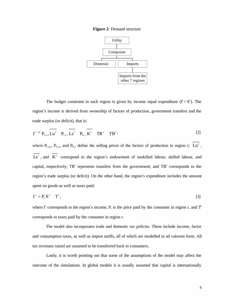
Figure 2: Demand structure

Domestic

Imports from theother 7 regions

Imports

Composite

Utility

The budget constraint in each region is given by income equal expenditure (Ir = Er). The

region’s income is derived from ownership of factors of production, government transfers and the

trade surplus (or deficit), that is:

rrrr,K

rr,Ls

rr,Lu

r TBTRKPLsPLuPI ++++= , [2]

where PLu,r, PLs,r, and PK,r define the selling prices of the factors of production in region r; Lu r ,

Lsr , and K r correspond to the region’s endowment of unskilled labour, skilled labour, and

capital, respectively; TRr represents transfers from the government; and TBr corresponds to the

region’s trade surplus (or deficit). On the other hand, the region’s expenditure includes the amount

spent on goods as well as taxes paid:

rrr

r TXPI += , [3]

where Ir corresponds to the region’s income, Pi is the price paid by the consumer in region r, and Tr

corresponds to taxes paid by the consumer in region r.

The model also incorporates trade and domestic tax policies. These include income, factor

and consumption taxes, as well as import tariffs, all of which are modelled in ad valorem form. All

tax revenues raised are assumed to be transferred back to consumers.

Lastly, it is worth pointing out that some of the assumptions of the model may affect the

outcome of the simulations. In global models it is usually assumed that capital is internationally

7

immobile. This assumption may not be very realistic since international capital markets are

becoming more integrated. However, this assumption is fundamental to the structure of the model;

if all factors of production are allowed to move freely, the concept of region is no longer clear.

Hence the need for a fixed factor in the specification of the model (in one of the extensions of the

model, when capital is assumed to be internationally mobile, unskilled labour is the fixed factor in

the model) 4.

Regarding labour, in the model it is assumed that differences in the marginal product of

labour arise from barriers to inward mobility of labour in high-wage countries. Thus, once barriers

to labour mobility are eliminated wage rates equalise across regions. The model also assumes that

labour in one region is the same as labour in another region, so that differences in labour quality or

human capital per worker across countries are ignored. In the real world these differences are not

only present but may also be significant. For example, Lucas (1995) indicates that production per

worker in the US is about fifteen times what it is in India; after correcting for differences in human

capital, each American worker was estimated to be the equivalent of about five Indian workers.

Another important factor that may affect labour productivity is the technology available in each

region. Thus, the elimination of restrictions on labour mobility may not after all eliminate

differences in productivity across regions. As can be seen, some of the assumptions used in the

specification of the labour market may be highly simplified; however, incorporating differences in

the quality of labour across regions is severely constrained by data availability.

2.2. EQUILIBRIUM CONDITIONS OF THE MODEL

Once the model has been specified, it can be solved for an equilibrium solution. Equilibrium in the

model is given by a set of goods and factor prices for which all markets clear. That is, demand-

4 Instead of having a fixed factor, a nontradable good could be introduced, so that all production factors couldbe inter-regionally mobile.

8

supply equalities hold in each goods and factors markets; zero profit conditions hold for each

industry in each region; and each region is in external-sector balance.

In the goods market, gross output equals final demand because intermediate production is

netted out; specifically, the model has the following blocks of market clearing conditions:

• The supply of goods for domestic consumption must equal the demand for domestically

produced goods.

• Exports from region r to region s must equal imports of region s from region r, because there

are assumed to be no transfer (e.g. transport) costs in shipping goods from one region to

another.

• Total supply of composite commodities, which consists of the composite of similar domestic

products and aggregate imports, must equal consumer’s demand in each region.

When labour is assumed to be heterogeneous, there is an additional market clearing

condition, which states that the supply of the aggregate labour input generated by the combination

of Lu and Ls, must equal the demand for the aggregate labour input used in the production of value

added.

As to the equilibrium conditions in the factor markets, we initially assume that all factors

are internationally immobile. This assumption implies that factor prices are different in each region;

this is an important assumption for the results of our model, since market clearing conditions in

factor markets determine factor prices. Under this assumption, we have separate labour and capital

equilibrium conditions in each region. That is, the region’s endowment of capital and labour must

equal factor use (i.e. full employment occurs in all regions). In the second variant of the model

capital is assumed to be internationally mobile. This assumption implies that there is only one price

for capital in the model, and this is determined by the market clearing condition that factor use

across all industries and regions must equal the world endowment of capital.

The zero profit conditions state that the total value of sales must equal the industry’s costs,

they must hold in each region. In particular,

9

• In each region the value of domestic output must be equal to the capital and labour costs of

producing the good. At the same time, the value of domestic output equals the value of

commodities sold in the domestic market plus the value of commodities sold as exports.

• The value of commodities sold as exports must equal the value of the sum of exports to the

other 7 regions.

• The value of total imports must equal the value of the sum of imports from the other 7 regions.

• The value of the composite commodity demanded by consumers must equal the value of

aggregate imports plus the value of domestically produced goods.

• The value of goods sold for domestic consumption must be equal to the value of the demand for

domestically produced goods.

• The value of exports from region r to region s must be equal to the value of imports of region s

from region r.

Once again, when considering heterogeneous labour it is necessary to introduce an

additional zero profit condition, that the value of the aggregate labour input must be equal to the

skilled and unskilled labour costs of producing the aggregate input.

Finally, the external sector balance condition indicates that each region is always on its

budget constraint. In this case, we assume that in each region the value of exports minus the value

of imports, that is the trade surplus (or deficit), remains fixed in real terms.5

rrX

rrrM EXPPTBIMPP =+ [4]

where

= r0

r

rrr

0r

XPXP

TBTB , where 0rP is the benchmark consumer price (this price is equal to 1), TB r

0 is

the benchmark trade surplus (or deficit), and the term in parentheses is a Paasche price index. We

use this price index to take into account changes in prices in the new equilibrium.

5 We do not have a zero trade balance, since this involves adjusting the data.

10

Once the equilibrium conditions that characterise the model have been specified, we

proceed to compare counterfactual equilibria with the benchmark equilibrium generated by the data.

However, before doing this, we calculate the parameters of the model that are consistent with the

benchmark data set; these parameters allow us to reproduce the data set as an equilibrium solution

of the model.

3. EMPIRICAL IMPLEMENTATION

The model consists of eight regions, each of which engages in domestic and foreign trade activities.

These regions were chosen to reflect world trade, and we use 1990 data for the United States

(USA), Japan (JAP), the European Union (12-member-EU), other development countries (ODC),

developing America (DAM), developing Africa (DAF), developing Asia (DAS), and developing

Europe (DE).6 Table 1 presents the grouping of individual countries.

We assume that each region produces one commodity, and that each region’s domestically

produced and imported goods are qualitatively different (Armington, 1969). We consider one

commodity as our analysis focuses on the efficiency gains from the elimination of restrictions on

labour mobility. The introduction of a segmented labour market is a very important feature of our

model, so that we consider two types of labour: skilled and unskilled. This characteristic allows as

to analyse the distributional effects that the migration of skilled labour has on unskilled labour,

since the assumption of homogeneous labour implies that the benefits and losses of migration are

evenly distributed within each region. Lastly, the price of the composite commodity demanded by

the consumer in USA is chosen as the numeraire.

6 Initially, developing Oceania (which included Fiji, Kiribati, Papua New Guinea, Samoa, Solomon Islands,and Vanuatu) was included as a ninth region. At the time of solving the model we encountered numericalproblems because this region was very small compared to the others (in 1990 its GDP accounted for only0.2% of world GDP). Hence, it was excluded from the analysis.

11

3.1. BENCHMARK DATA SET

The benchmark data set involves domestic activity data and external sector data for each region in

1990. Domestic activity data involve data on value added by component, the segmentation of the

labour market as well as domestic taxes. External sector data includes data on foreign trade and

import tariffs.

The size of the eight regions is given by their respective GDP in 1990 US dollars,

consistent with the World Tables (1995). The benchmark data set satisfies the equilibrium

conditions of the model in the presence of the existing policies. We use data from National

Accounts as compiled by the United Nations, World Tables produced by the World Bank, and the

Government Finance Statistics Yearbook of the International Monetary Fund. Regarding foreign

trade statistics, we use information from UNCTAD (1995) and the GATT-trade policy review for

various countries.

The data set used was based on a data set previously assembled by the author, in which

each region produced three goods, namely primary commodities, manufactured goods, and services.

For the purpose of this paper, these three goods were aggregated into a single commodity. We use

information from (various issues of) the Yearbook of Labour Statistics of the International Labour

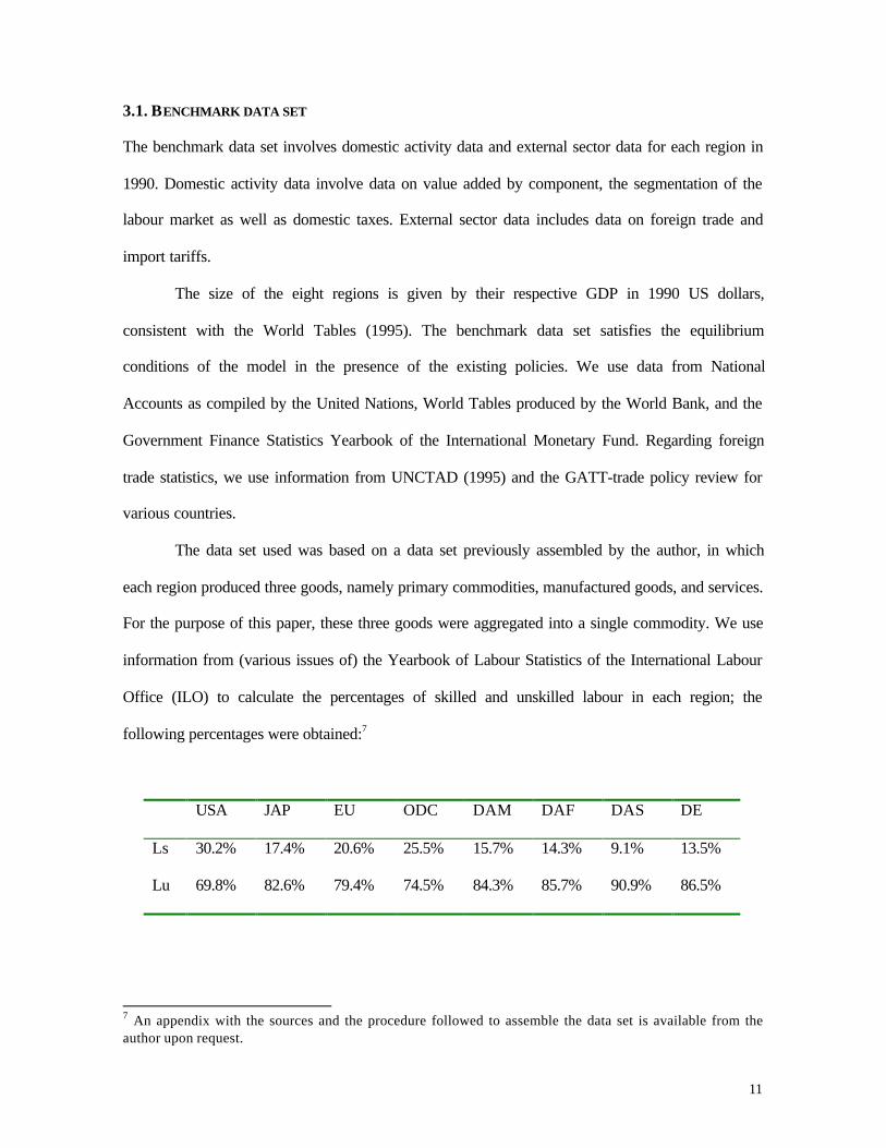
Office (ILO) to calculate the percentages of skilled and unskilled labour in each region; the

following percentages were obtained:7

USA JAP EU ODC DAM DAF DAS DE

Ls 30.2% 17.4% 20.6% 25.5% 15.7% 14.3% 9.1% 13.5%

Lu 69.8% 82.6% 79.4% 74.5% 84.3% 85.7% 90.9% 86.5%

7 An appendix with the sources and the procedure followed to assemble the data set is available from theauthor upon request.

12

As can be seen, these percentages indicate that more than 17% of the labour force in

developed regions is skilled, while in developing regions this percentage is less than 16%. National

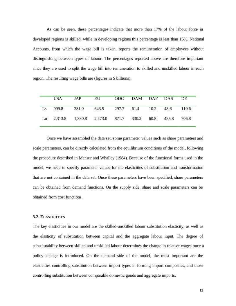
Accounts, from which the wage bill is taken, reports the remuneration of employees without

distinguishing between types of labour. The percentages reported above are therefore important

since they are used to split the wage bill into remuneration to skilled and unskilled labour in each

region. The resulting wage bills are (figures in $ billions):


Ls 999.8 281.0 643.5 297.7 61.4 10.2 48.6 110.6

Lu 2,313.8 1,330.8 2,473.0 871.7 330.2 60.8 485.8 706.8

Once we have assembled the data set, some parameter values such as share parameters and

scale parameters, can be directly calculated from the equilibrium conditions of the model, following

the procedure described in Mansur and Whalley (1984). Because of the functional forms used in the

model, we need to specify parameter values for the elasticities of substitution and transformation

that are not contained in the data set. Once these parameters have been specified, share parameters

can be obtained from demand functions. On the supply side, share and scale parameters can be

obtained from cost functions.

3.2. ELASTICITIES

The key elasticities in our model are the skilled-unskilled labour substitution elasticity, as well as

the elasticity of substitution between capital and the aggregate labour input. The degree of

substitutability between skilled and unskilled labour determines the change in relative wages once a

policy change is introduced. On the demand side of the model, the most important are the

elasticities controlling substitution between import types in forming import composites, and those

controlling substitution between comparable domestic goods and aggregate imports.

13

The majority of studies on labour-labour substitution use a disaggregation by occupation to

separate the labour force; in particular, the disaggregation most widely used is between production

and non-production workers, because of data availability. There does not seem to be consensus as to

an approximate value for the labour-labour substitution elasticity, and this is reflected by the fact

that there is a rather large range of variation in the elasticity estimates, from 0.14 to 7.5

(Hamermesh and Grant 1979).8 The big differences in the elasticity estimates can be the result of

major methodological differences, such as the choice of estimating a cost or a production function,

the choice of functional forms, the choice of data (time-series versus cross-section), and the

disaggregation of the labour force according to various criteria, among others. The estimate of the

elasticity of substitution between non-production-production workers was chosen as proxy for the

elasticity of substitution between skilled and unskilled labour. We use a value of 0.9 in our central

case, and this value is used for all regions, since estimates for each region were not available.

Sensitivity analysis is performed around the value chosen in the range 0.5 to 2.5.9

In the case of the value added functions, the key parameters are the CES elasticities of

substitution between the aggregate labour input and capital. 10 We use elasticities of factor

substitution based on those used by Whalley (1985). Because of the lack of detailed regional data

our elasticities are almost identical across regions.

On the demand side of the model, two different types of elasticities are involved with the

CES forms used: those controlling substitution between import types in forming import composites,

and those controlling substitution between comparable domestic goods and aggregate imports. In

this model, elasticities of substitution in consumption are not needed because each representative

8 Hamermesh (1993), however, points out that the substitution relationship between production and non-production workers tells us little about the substitution between high- and low-skilled workers because“…there is a remarkably large overlap in the earnings of these two groups” (p. 65).9 It was also tried to use elasticity values greater than 2.5, but we encountered numerical problems whensolving the model.10 Whalley (1985) points out that there is no consensus as to the quantitative orders of magnitude involved,since most time-series estimates of the aggregate substitution elasticity are in the neighbourhood of unity, andcross-section estimates are often around 0.5.

14

consumer demands one good only, which is a composite of comparable domestic and imported

(composite) goods.

Regarding trade elasticities, the most important are import-price elasticities and export-

price elasticities. Substitution elasticities between import types making up any composite determine

the export-price elasticities faced by regions. Substitution elasticities between import composites

and comparable domestic products reflect import-price elasticity estimates in the literature, since it

was not possible to find any econometric estimate of elasticities of substitution. The elasticities used

in the model (central case) are presented in Table 2.

3.3. CALIBRATION

Once the data set has been assembled, and elasticity parameters have been specified, share and scale

parameters can be calculated from the equilibrium conditions of the model, following the procedure

described in Mansur and Whalley (1984).

The benchmark data set provides information on equilibrium transactions in value terms.

The first step of the calibration procedure involves the separation of these transactions into price

and quantity observations. In order to do this, a units convention is widely used, in which it is

assumed that a physical unit of each good and factor is the amount that sells for one dollar. That is,

both goods and factors have a price of unity in the benchmark equilibrium.

However, this approach is not applicable in the case of the labour market, because we

assume different marginal products of labour, resulting from barriers to inward mobility of labour in

high-wage countries (that is, wages are different from one). In addition, we consider two types of

labour, skilled and unskilled, each one with a different productivity and, as a result, a different price

within each region.

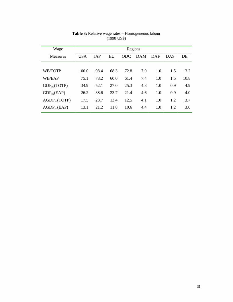
There is no agreement as to how to calculate the average wage rate. Hence, we consider six

alternative measures, which are the most widely used. First, we use the wage bill for each region

(WB), as taken from National Accounts, and divide it by total population (TOTP), as taken from the

15

UN Demographic Yearbook. Total population, however, exceeds the workforce in each region.

Therefore, we use as a second measure of the average wage rate the wage bill divided by the

economically active population (EAP).11 The third and fourth measures use GDP per capita using

TOTP and EAP, respectively. The fifth and sixth measures of the average wage rate use GDP per

capita using TOTP and EAP, where the GDP has been adjusted by the exchange rate deviation

index, that corrects for the difference between the official and the purchasing power parity exchange

rates (AGDPpc) (Kravis et al., 1982). The wage measures based on GDP per capita were included

for comparison purposes, since Hamilton and Whalley (1984) used this measure in their

calculations. However, GDP per capita in only an approximate measure of average wages as it is a

measure of economic activity, and not a measure of income. Furthermore, in the production of

domestic output labour is not the only factor of production involved; physical capital and human

capital are also involved. From GDPpc it is not possible to isolate the labour component. Table 3

reports the relative wage rates calculated using the six alternatives mentioned above. Regardless of

how the wage rates are calculated, USA, JAP, EU and ODC have higher wage rates than the

developing world (i.e. DAM, DAF, DAS and DE).

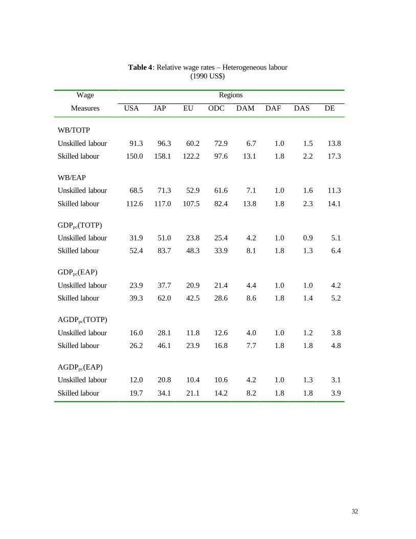
When there is labour market segmentation, we need to calculate the average wage rates of

skilled and unskilled labour in each region. Given that in practice such data are not available, we

use average earnings per worker in finance, insurance, real state and business services as proxy for

skilled labour wages, while average earnings per worker in wholesale and retail trade, restaurants

and hotels as proxy for unskilled labour wages. The ratio between high and low wages is then used

to infer the average wage rates for skilled and unskilled labour in each region. 12 The resulting

relative wage rates for the two types of labour are reported in Table 4.

11 ILO (1996; p.5) defines the economically active population as “…all persons of either sex who furnish thesupply of labour for the production of goods and services during a specified time-reference period”.12 An appendix with the procedure followed to calculate average wage rates is available from the author uponrequest.

16

The final step in the calibration procedure is to use the price-quantity data to calculate

parameters for demand and production functions from the benchmark equilibrium observations,

given the required values of pre-specified parameters such as elasticities and tax rates. In order to do

this, we use the equilibrium conditions together with first-order conditions (from utility

maximisation and cost minimisation), to solve for function parameter values using equilibrium

prices and quantities. Calibration allows us to test the solution procedure, and ensures the

consistency of agents’ behaviour with the benchmark data set. The model was solved using a

routine we wrote in the General Algebraic Modelling System (GAMS) software.

4. MODEL RESULTS

The model described above was used to calculate the world-wide efficiency gains from free

mobility of labour (the results are presented for the six measures of wages mentioned above). We

consider two scenarios: in the first one labour is a homogeneous factor of production, while in the

second one labour is classified as skilled and unskilled. In the latter scenario, we consider two

cases: a) both skilled and unskilled labour migrate; and b) skilled labour is the only factor that

migrates. We did not consider the case where unskilled labour is the only factor that migrates since

this is not a realistic case, given the actual international restrictions on labour mobility. The model

does not consider illegal migration.

The removal of restrictions on labour mobility modifies the market clearing condition that

determines the equilibrium wage rate. In particular, when labour is homogeneous the equilibrium

condition is given by

∑∑==

=8

1r

r8

1r

r LL , [5]

where rL corresponds to the region’s endowment of labour. In the heterogeneous case we have

∑∑==

=8

1r

r8

1r

r LsLs , [6]

17

where rLs corresponds to the region’s endowment of skilled labour.

In the model international capital transfers are not considered, since it is assumed that

migrant workers do not bring capital with them nor send capital back home. Capital flows and

transfers may alleviate the negative effects of migration on wages. In addition, the model assumes

that all migrant labour enter the labour market (some migrants such as children and elderly people

will not actually work).

Once immigration controls are removed, labour migrates from low-wage regions to high-

wage regions. The source regions are DAM, DAF, DAS, and DE, while the destination regions are

USA, JAP, EU, and ODC. However, when the average wage rate is measured as wage bill divided

by EAP, and wage bill divided by TOTP, DE becomes a destination region for the homogeneous

labour case. When labour is heterogeneous, and both skilled and unskilled labour migrate, DE

becomes a destination region for unskilled labour, and a source region for skilled labour. Regardless

of whether labour is homogeneous or heterogeneous, the amount of the factor entering DE is not

considerable.

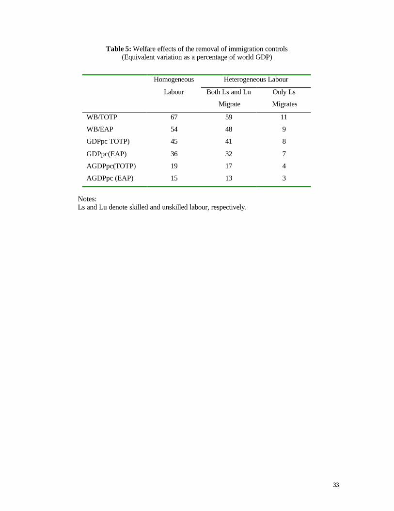
Table 5 quantifies the effects of the removal of immigration controls on welfare, as

measured by the aggregate equivalent variation. 13 In the homogeneous labour case, there is a

reduction in production in all sectors in the source regions. This is accompanied by a reduction in

exports and an increase in imports which compensate for the reduction in domestic output.

Conversely, in the destination regions, there is an increase in production in all sectors accompanied

by an increase in exports and a reduction in imports from developing regions. In this case, there are

large gains from the removal of global immigration controls, ranging from 15% to 67% of world

GDP. These gains are not as large as those obtained by Hamilton and Whalley (1984), where in

some cases the gains exceeded the world-wide economy GNP. The differences may be the result of

13 The equivalent variation (EV) is a measure of welfare change. It is defined as the amount of money aparticular change, that has taken place between equilibria, is equivalent to. In this case, an arithmetic sum ofEVs, summed across regions is used.

18

the modelling frameworks (i.e. partial equilibrium versus general equilibrium), the flows of labour

leaving low-wage regions, or units of measurement as Hamilton and Whalley (1984) use

population, and we use units of labour.

Table 5 also presents the welfare effects of the removal of immigration controls when

labour is a heterogeneous factor. In this case, as in the previous scenario with homogeneous labour,

there is an increase in domestic output in developed regions, whereas output reduces in developing

countries; the reduction in domestic output is compensated by a reduction in exports and an increase

in imports from developed regions. When both skilled and unskilled labour migrate, efficiency

gains range from 13% to 59% of world GDP. The gains are smaller than in the homogeneous case

as a result of the technological constraint imposed by the substitutability between skilled and

unskilled labour. Thus, with a segmented labour market skilled and unskilled labour have less

opportunity to reallocate. When only skilled labour migrates, world-wide welfare gains are much

smaller than in the previous two cases (from 3% to 11% of world GDP) because skilled labour

represents a small fraction of the labour force in the source regions (i.e. 14% in DAM, 10% in DAF,

5% in DAS, and 14% in DE).

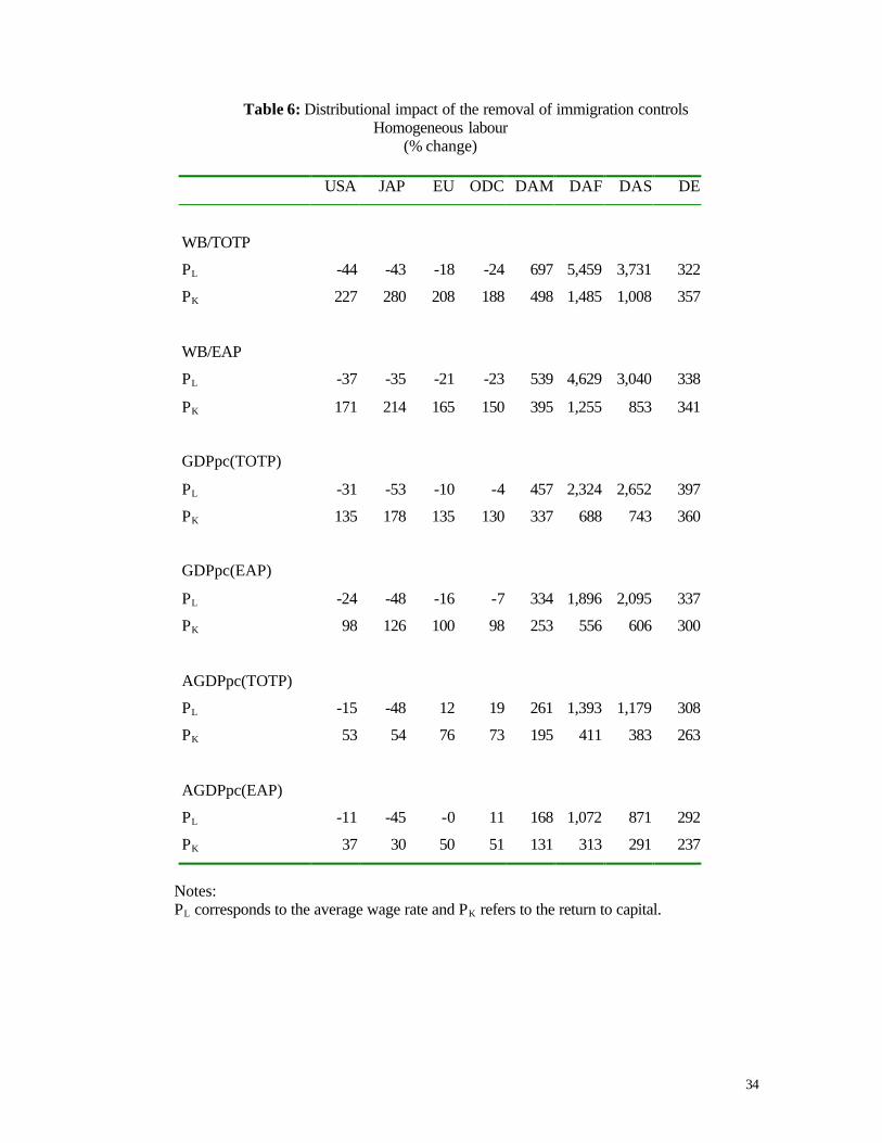
The segmentation of the labour market also allows us to examine the distributional effects

of immigration between skilled and unskilled labour in each region. Tables 6 to 8 present the

distributional impacts of the removal of immigration controls for the six measures of wages

considered. A priori one would expect that labour migration from the source regions increases the

labour supply in the destination regions, reducing the average wage rate (assuming no rigidities),

and benefiting capital owners. In the source regions, the removal of immigration controls is

expected to reduce the labour supply, increasing the average wage rate. As a result, capital is less

scarce relative to labour, so that a reduction in the return to capital is expected.

In the case of homogeneous labour, capital owners in the destination regions indeed benefit

from migration, despite the fact that for some regions the average wage rate increases (in these

19

cases, the return to capital increases even more). In the source regions workers are better off as a

result of migration and capital owners lose (Table 6).

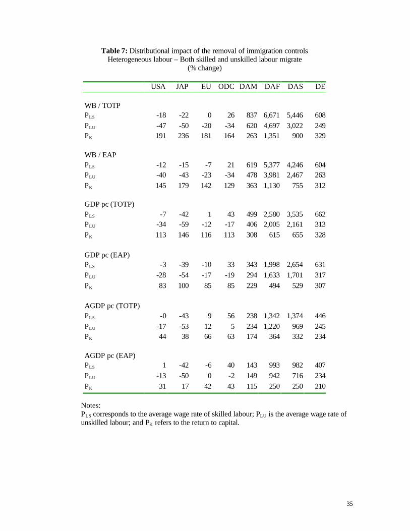
Let us now consider the case of heterogeneous labour (see Tables 7 and 8). When both

skilled and unskilled labour migrate, average wages increase in the source regions because labour is

less abundant relative to capital, and the return to capital decreases. The removal of immigration

controls benefits skilled labour more than unskilled labour, because the former is a small proportion

of the total labour force, and after migration this factor is more scarce in developing regions. In the

destination regions average wages reduce for both skilled and unskilled labour, since labour is now

less scarce relative to capital, and the return to capital increases.

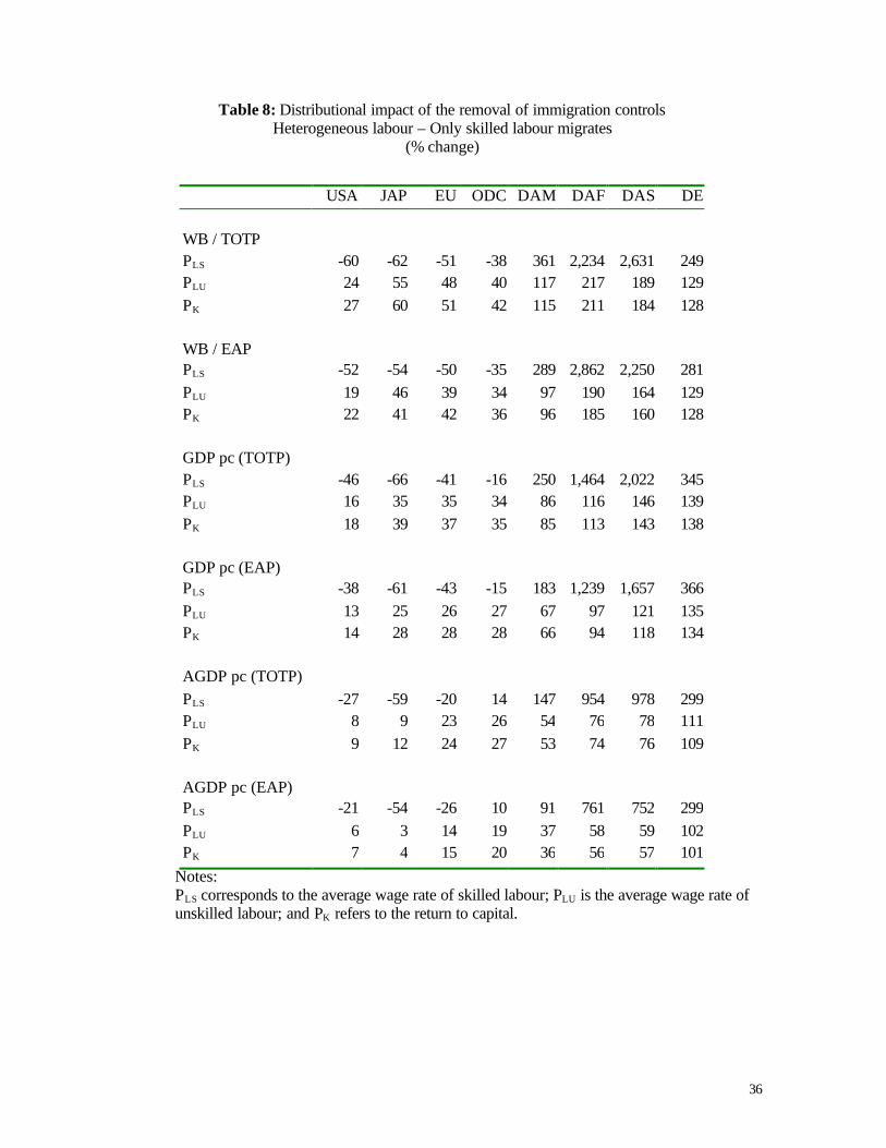
When only skilled labour migrates, there is a substantial increase in the remuneration of this

type of labour in the source regions, since this factor of production is not abundant in these regions.

Unskilled workers and capital owners are worse off as a result of migration, despite the fact that

there is an increase in their remuneration. As to the destination regions, the inflow of skilled labour

increase the supply of this type of labour, hence reducing its average wage rate. As we would

expect, the average wage of unskilled labour and the return to capital increase. Skilled labour is

worse off.. The flexibility of wages allows the labour market to absorb labour immigration. Lower

wages induce an increase in labour demand and in aggregate employment.

The amount of labour leaving the source regions varies depending on the measure used to

calculate average wages. For example, when these are measured as the wage bill divided by TOTP,

53% of the labour endowment of developing regions migrate to developed regions; when the

average wage rate is measured as adjusted GDP per capita using EAP, this percentage reduces to

37%. On the other hand, when both skilled and unskilled labour migrate in the heterogeneous

labour case, the percentage of labour leaving the source regions varies from 35% (average wage rate

measured as adjusted GDP per capita using EAP) to 50% (average wage rate measured as the wage

bill divided by TOTP). When only skilled labour migrates, between 59% and 73% of the skilled

20

labour endowment of developing regions migrate, depending on how the average wage rate is

calculated.

In summary, migration leads to factor reallocation, and during this process there are

winners and losers. In the source regions, labour becomes more scarce relative to capital (between

37% and 53% of the labour endowment of developing regions migrate to developed regions,

depending on the wage measure used), and capital owners lose. However, not all workers are better

off, since labour is a heterogeneous factor. Emigration will benefit workers whose skills are

substitute to those of migrant labour, whereas it will hurt those workers whose skills are

complementary to those of migrant workers. On the other hand, in the destination regions, labour

becomes more abundant (less scarce) relative to capital, so that capital owners benefit. However,

not all workers are worse off, because labour is a heterogeneous factor. Immigration will benefit

those workers whose skills are complementary to those of the immigrant worker, whereas

immigration will hurt those workers whose skills are substitute to those of immigrant workers.

We also performed a sensitivity analysis on the key elasticities of the model.14 In particular,

in a first set of simulations the elasticity of labour-labour substitution was varied from 0.5 to 2.5.

This elasticity is very important in our model since it includes a segmented labour market, a feature

that has not been considered in previous works. In a second set of simulations, the elasticities of

substitution in the production of value added were set at values between 0.5 and 1.5 in all regions.

When labour is homogeneous, this substitution elasticity corresponds to the elasticity of substitution

between capital and labour; when labour is heterogeneous, it corresponds to the elasticity of

substitution between the aggregate labour input and capital. We conclude that the results are robust

to the elasticity choice, in the sense that the elimination of immigration controls generates world-

wide efficiency gains. In addition, in the destination regions capital owners benefit from labour

immigration, and workers lose because of lower wages. In the source regions, capital owners are

14 The results are not reported here, but are available from the author upon request.

21

worse off and workers are better off. When the labour market is segmented, the sensitivity analysis

also confirms that migration of skilled labour hurts unskilled labour in the source regions.

5. MODEL EXTENSIONS

This section introduces three new features to the model: a) transaction costs; b) international capital

mobility; and c) selective labour mobility. For brevity we only report the results of two out of the

six measures of average wages considered: average wage rate as measured by the wage bill divided

by TOTP, and as adjusted GDP per capita using EAP. These two measures were chosen as they

provided the extreme results.

5.1. TRANSACTION COSTS

The first elaboration of the model is the introduction of transaction costs. This extension of the

model seems appropriate, since migration is a costly process. There are costs involved in the

process of moving from one region to another, such as transport costs, the costs of settling in other

region, the costs of finding a new job, and the costs of leaving friends and family behind. With the

elimination of restrictions on labour mobility, labour will move until the marginal product of labour

equals the cost of hiring labour. However, in the presence of transaction costs, wages fail to equalise

across regions; hence, a single market clearing wage no longer characterises the equilibrium.

Transaction costs thus drive a wedge between wages in developed and developing countries.

Migration flows reduce compared to the case without transaction costs.

Transaction costs were modelled as a tax (without revenue), whose rate is exogenously

determined. The price received by owners of labour in each region corresponds to a percentage of

the market clearing price when restrictions to labour mobility are eliminated. That is, the price of

labour in each region is given by,

P W TCLr r= −( )1 , [7]

22

where W corresponds to the world price of labour, and TCr corresponds to regional transaction

costs.

Transaction costs are difficult to quantify since there are no measures available. As

mentioned earlier, there are costs associated with migration from low-wage to high-wage regions. In

the case of developing regions, these costs could be very high. Taking into account the substantial

differences in relative wages among the regions, we assume the following values for transaction

costs: 0.9 for DAF and DAS; 0.8 for DAM; and 0.7 for DE. The transaction costs for developed

regions (USA, JAP, EU, and ODC) are assumed to be much smaller (i.e. 0.1), since workers in

these regions have little or no incentive to move to low-wage regions.

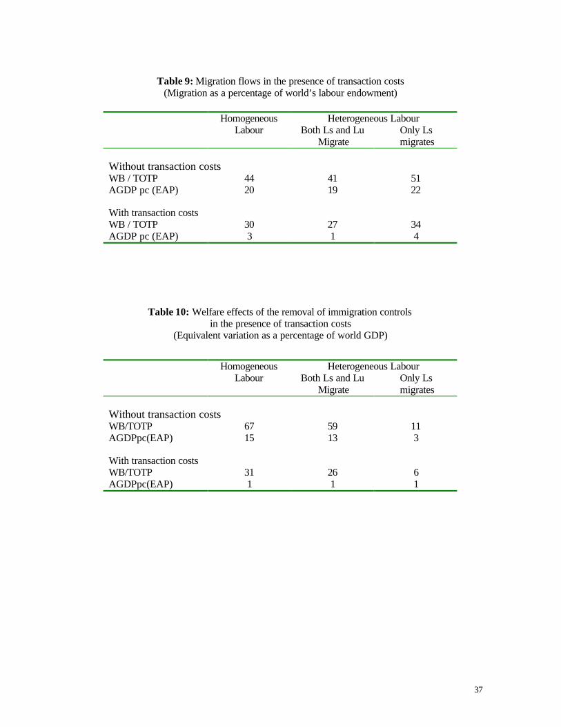
The introduction of transaction costs reduces migration flows (see Table 9). For example,

when the average wage is measure as the wage bill divided by TOTP, and labour is homogeneous,

migration reduces from 44% of the world endowment of labour to 20%. In the heterogeneous labour

scenario, migration reduces from 41% of the world endowment of labour to 27% when the two

types of labour are allowed to migrate, and from 51% of the world endowment of labour to 37%

when only skilled labour migrates.

The welfare gains as a result of the removal of immigration controls are smaller in the

presence of transaction costs (see Table 10). Regarding the distributional effects, the main

conclusions remain unaltered. That is, labour benefits (loses) relative to capital in the source

(destination) regions. When the labour market is segmented, skilled labour benefits relative to

unskilled labour in the source regions; in the destination regions the two types of labour lose, but

unskilled workers are hurt even more when both skilled and unskilled labour migrate.

Finally, migration and welfare gains increase as the transaction costs for the developing

regions are reduced (these results are not reported here). This is the case since transaction costs

distort the labour market, specially in developing regions, and as the distortion is reduced,

efficiency increases and the wage gap reduces.

23

5.2. CAPITAL MOBILITY

In the second elaboration of the model we introduce international capital mobility. Although this

feature is usually ignored in global models (see e.g., Whalley, 1985; Shoven and Whalley, 1992), it

seems interesting to include it in the model since capital markets are becoming more integrated

internationally. In this case, the return to capital equalises across regions. Therefore, a single market

clearing rental rate characterises the equilibrium; that is, the market clearing condition for the

market of the capital factor is given by,

∑∑==

=8

1r

r8

1r

r KK , [8]

that is the sum of the demand for capital in each region must equal the global endowment of the

factor.

Simulations were carried out for the scenario in which we have heterogeneous labour and

only skilled labour migrates, since we need a fixed factor (in this case unskilled labour). If all

factors of production are allowed to move freely, the concept of region is no longer clear.

When we remove the restrictions to skilled labour mobility, we observe that labour moves

from regions with low wages (DAM, DAF, DAS, and DE) to regions with high wages (USA, JAP,

EU, and ODC). Capital moves from regions where it is abundant relative to labour (USA, JAP, EU,

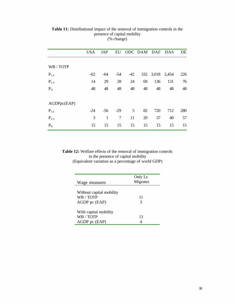
and ODC) to regions where it is scarce relative to labour (DAM, DAF, DAS, and DE). The effects

over the remuneration of the factors of production are similar to those obtained when capital is not

internationally mobile. We observe a substantial increase in the remuneration of skilled labour in

the source regions, since this factor is not abundant in these regions, whereas unskilled labour and

capital owners are worse off; in the destination regions, the remuneration of skilled labour falls and

unskilled labour and capital owners are better off (see Table 11). The effects of capital mobility on

the return to capital are smaller than the effects of skilled labour mobility on wages. This is

explained by the fact that capital flows from developed to developing regions are smaller than

labour flows from developing to developed regions. In particular, when wages are measured as the

24

wage bill divided by TOTP, migration flows account for 56% of the world endowment of labour

whereas capital flows account for only 7% of the world endowment of capital.

In addition, aggregate welfare improves compared with the scenario without capital

mobility (see Table 12). The improved welfare is the result of a better resource allocation with

smaller distributional effects.

The previous results should be taken with caution since they are ruled by the specification

of the capital market. That is, since we assume a competitive market, capital will respond to

variations in its rate of return. However, as indicated by Layard et al (1992), developing regions

have low productivity, and it is possible that migration from DAM, DAF, DAS, and DE to USA,

JAP, EU, and ODC would divert capital to developed regions that could be instead invested in

developing regions.15

5.3. SELECTIVE LABOUR MOBILITY

The third elaboration of the model is the introduction of selective labour mobility. This extension

seems interesting since some countries have signed bilateral agreements with other countries that

cover project-link work, seasonal work, work in border areas, and guest workers.16 We focus on the

case where individuals in some particular regions in the developing world are allowed to migrate to

developed regions. We consider the following seven possibilities:

• Workers in DAM migrate to USA, JAP, EU, and ODC.

• Workers in DAF migrate to USA, JAP, EU, and ODC.

• Workers in DAS migrate to USA, JAP, EU, and ODC.

• Workers in DE migrate to USA, JAP, EU, and ODC.

• Workers in DAM migrate to USA.

15 Lucas (1995) provides an alternative explanation.16 For example, Germany have signed labour agreements with Hungary, Poland, and the Czech Republic.Also Belgium, France and Switzerland have signed labour agreements with East European countries(Weyerbrock, 1995)

25

• Workers in DAS migrate to JAP.

• Workers in DAF and DE migrate to EU.

Each of these seven possibilities are analysed when labour is homogeneous, when labour is

heterogeneous and both skilled and unskilled workers migrate, and when labour is heterogeneous

and only skilled workers migrate.

Under this elaboration, the average wage equalises across the regions involved, whereas

each of the excluded regions will have a market clearing condition for the labour market.

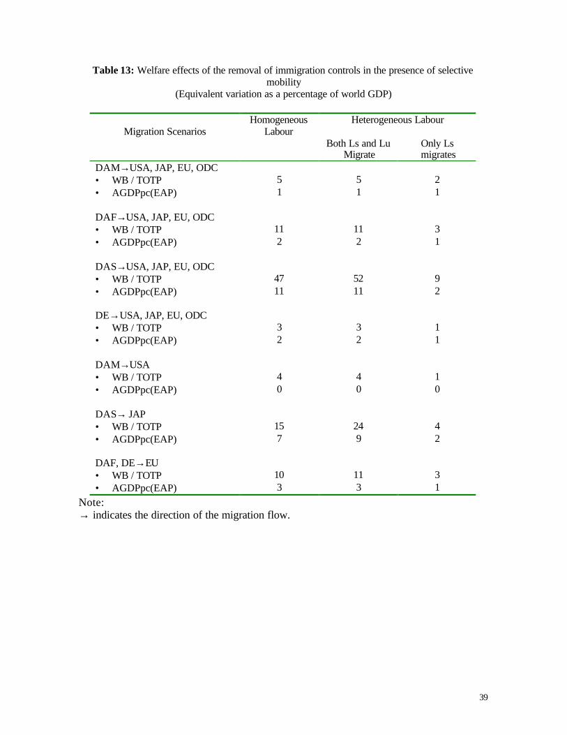
We observe an aggregate welfare improvement in all seven cases (see Table 13). The

magnitude of the welfare gains depends on the size of the source region in terms of the labour

market endowment. In particular, the highest welfare gains are obtained when workers in DAS are

allowed to migrate to USA, JAP, EU, and ODC, since DAS is the most densely populated region,

and has one of the lowest average wages. Conversely, the lowest welfare gains are obtained when

DE is allowed to migrate to USA, JAP, EU, and ODC; this result is not surprising since DE is the

third region in terms of population in the developing world, and the region’s average wages are, in

some cases, the highest in then developing world.

In terms of the amount of labour that moves between regions, the largest movement occurs

when workers in DAS are allowed to migrate to USA, JAP, EU, and ODC. In the homogeneous

case, the proportion of labour that moves out of DAS varies between 13% and 30% of the world

endowment of labour; in the heterogeneous labour case, the proportion of labour that moves out of

DAS varies between 12% and 36% of the world endowment of labour. Conversely, the smallest

amount of migration occurs when the workforce in DE is allowed to migrate to USA, JAP, EU, and

ODC. These results suggest a positive relationship between the amount of migration and welfare

gains.

As to the distributional impact of the removal of immigration controls, results not reported

here indicate that the introduction of selective labour mobility does not affect our main conclusions

in the homogeneous labour case (i.e. workers in the source region and capital owners in the

26

destination regions benefit from migration). However, the magnitude of the distributional effects

tend to be smaller in the destination regions, and larger in the source regions.

Let us now consider the heterogeneous labour case with skilled and unskilled labour

migration. To begin with, when workers in DAM migrate to USA, JAP, EU, and ODC, skilled

labour in ODC also migrates to the other developed regions because the remuneration of this factor

is the lowest of the developed world.17 Skilled and unskilled labour are better off relative to capital

in the source regions, and in DAM unskilled labour is better off relative to skilled labour. This

result contrasts with the findings in the central case, and can be explained by the fact that more

unskilled labour is migrating out of the region. In the other selective labour mobility cases, skilled

labour is better off relative to unskilled labour and capital in the source regions, whereas in the

destination regions unskilled labour is worse off relative to skilled labour, and capitalists benefit.

Lastly, when we have a segmented labour market and skilled labour migration, skilled

workers gain in the source regions relative to unskilled workers; in the destination regions, both

unskilled and skilled labour lose relative to capital, although unskilled labour loses less than skilled

labour.

6. CONCLUDING REMARKS

In this paper we have computed the world-wide efficiency gains from the elimination of restrictions

on labour mobility. One of the key features of our model is the introduction of a segmented labour

market, as we consider two types of labour, skilled and unskilled. When labour is heterogeneous,

we consider the cases where both skilled and unskilled labour migrate, and when only skilled labour

migrates. In our analysis, wages differ across regions because of the existence of barriers to labour

mobility, and wage rates are equalised as a result of the elimination of restrictions to labour

mobility rather than free trade.

17 ODC also becomes a source of skilled labour when only workers in DAF, and only workers in DE areallowed to migrate to the developed world.

27

Our findings indicate that the elimination of global restrictions to labour mobility generates

world-wide efficiency gains, that could be of considerable magnitude, ranging from 15% to 67% of

world GDP. When only skilled labour is allowed to migrate welfare gains are smaller, since skilled

labour is a small proportion of the labour force in developing regions; in this case, efficiency gains

range from 3% to 11% of world GDP.

Migration also leads to a process of factor reallocation in which there are winners and

losers. In the source regions, labour becomes more scarce relative to capital, and capital owners

lose. However, not all workers are better off, since labour is a heterogeneous factor. Emigration will

benefit workers whose skills are substitute to those of migrant labour, whereas it will hurt those

workers whose skills are complementary to those of migrant workers. On the other hand, in the

destination regions, labour becomes more abundant (less scarce) relative to capital, and capital

owners benefit. Again, not all workers in the destination regions are worse off, because labour is a

heterogeneous factor. Immigration will benefit those workers whose skills are complementary to

those of the immigrant worker, whereas immigration will hurt those workers whose skills are

substitute to those of immigrant workers.

The model was then extended by including: a) transportation costs, since migration is a

costly process; b) capital mobility, since capital markets have become more international in scope;

and c) selective labour mobility, since some countries have introduced immigration control policies

that allow migration flows from some regions and not from others.

With the introduction of transaction costs, wages fail to equalise across regions, migration

flows reduce and in consequence efficiency gains reduce as well. With capital mobility, the return

to capital equalises across regions; the removal of restrictions to skilled labour mobility makes

labour move out of the regions with low average wages, and capital moves out of the regions where

it is abundant relative to labour. Global welfare improves compared with the scenario without

capital mobility, as a result of a better resource allocation and migrants benefit as well. With

selective labour mobility, aggregate welfare improves, and the magnitude of the gain depends on

28

the size of the region in terms of the labour endowment. As to distributional effects, labour benefits

in the source regions, and capital in the destination regions. With a segmented labour market, skill

labour benefits from migration relative to unskilled labour in the source regions.

Finally, our results have shown that the elimination of global restrictions to labour mobility

generates considerable world-wide efficiency gains. Despite these gains, the liberalisation of world-

wide migration is far from realistic because of social and political tensions. High-income countries

are very reluctant to open their borders to free migration because they do not want to become the

destination of immigration of unskilled labour from low-income countries. In the short-run,

countries regulate the flows of international migration by means of border controls, and work

permits, among others. In the long-run, countries should concentrate their efforts in the elimination

of the incentives to migrate, which could be accomplished by reducing income disparities among

regions.

29

Table 1: Regional classification Region 1: United States

USA Region 2: Japan

JAP Region 3: Belgium Denmark France Germany EU Greece Ireland Italy Luxembourg Netherlands Portugal Spain United Kingdom Region 4: Australia Austria Canada Finland ODC Iceland Israel New Zealand Norway South Africa Sweden Switzerland Region 5: Antigua & Barbuda Argentina Barbados Belize DAM Bolivia Brazil Chile Colombia Costa Rica Dominica Dominican Rep. Ecuador El Salvador Grenada Guatemala Guyana Haiti Honduras Jamaica Mexico Nicaragua Panama Paraguay Peru St. Lucia St.Kits & Nevis Suriname Uruguay Trinidad & Tobago Venezuela St. Vincent & the Grenadines Region 6: Algeria Angola Benin Botswana DAF Burkina Faso Burundi Cameroon Cape Verde Central African Rep. Chad Comoros Congo Cote d’Ivoire Djibouti Egypt Equatorial Guinea Ethiopia Gabon Gambia Ghana Guinea Guinea-Bissau Kenya Lesotho Madagascar Malawi Mali Mauritania Mauritius Morocco Mozambique Namibia Niger Nigeria Reunion Rwanda Sao Tome & Principe Senegal Seychelles Sierra Leone Sudan Swaziland Togo Tunisia Uganda Tanzania Zambia Zimbabwe Region 7: Bahrain Bhutan Bangladesh China DAS Hong Kong India Indonesia Iran (Islamic Rep) Jordan Kuwait Laos Lebanon Malaysia Mongolia Myanmar Nepal Oman Pakistan Philippines Qatar Rep. of Korea Saudi Arabia Singapore Sri Lanka Syrian Arab Rep. Taiwan Thailand Yemen United Arab Emirates

Region 8: Bulgaria Croatia Cyprus Czech Rep. DE Estonia Hungary Malta Poland Romania Slovenia Turkey USSR (former) Yugoslavia (former)

30

Table 2: Elasticities in the model

Elast. USA JAP EU ODC DAM DAF DAS DE ς 0.900 0.900 0.900 0.900 0.900 0.900 0.900 0.900 σ 0.830 0.800 0.820 0.840 0.850 0.860 0.840 0.840 π 0.920 0.930 0.859 0.948 1.263 1.019 1.546 2.715 ζ 0.990 0.930 0.919 1.130 0.544 0.572 1.227 1.410

Notes: ς is the labour-labour substitution elasticity. σ is the elasticity of substitution between capital and the aggregate labour input; based on estimatespresented in Whalley (1985). υ is the elasticity of substitution between domestic and imported goods. The values used are basedon import price elasticities. For USA and JAP the source is Marquez (1990). For EU we use anaverage of the elasticities of Germany and the United Kingdom (Marquez, 1990); France, Belgium-Luxembourg, Denmark, Ireland, Italy, and the Netherlands (Stern et. al., 1976); and Portugal(Houthakker and Magee, 1969). For ODC we use an average of the elasticities of Canada (Marquez,1990); Austria, Finland, Norway, Sweden, Switzerland, Australia, and New Zealand (Stern et. al.,1976). For DAM we use an average of the elasticities of Argentina, Brazil, Chile, Colombia, CostaRica, Ecuador, Peru and Uruguay (Khan, 1974). For DAF we use an average of the elasticities ofGhana and Morocco (Khan, 1974). For DAS we use an average of the elasticities of India, thePhilippines and Sri Lanka (Khan, 1974); and Pakistan and Bangladesh (Nguyen and Bhuyan, 1977).For DE we use the elasticity for Turkey estimated by Khan (1974). ζ is the elasticity of substitution between regional imports. The values used are based on exportprice elasticities. For USA and JAP the source is Marqez (1990). For EU we use an average of theelasticities of Germany and the United Kingdom (Marquez, 1990); France, Belgium-Luxembourg,Denmark, Ireland, Italy, and the Netherlands (Stern et. al., 1976); and Portugal (Houthakker andMagee, 1969). For ODC we use an average of the elasticities of Canada (Marquez, 1990); Austria,Finland, Norway, Sweden, Switzerland, Australia, and New Zealand (Stern et. al., 1976). For DAMwe use an average of the elasticities of Argentina, Brazil, Chile, Colombia, Costa Rica, Ecuador,and Peru (Khan, 1974). For DAF we use an average of the elasticities of Ghana and Morocco(Khan, 1974). For DAS we use an average of the elasticities of Pakistan, India, Bangladesh and SriLanka (Nguyen and Bhuyan, 1977). For DE we use the elasticity for Turkey estimated by Khan(1974).

31

Table 3: Relative wage rates – Homogeneous labour

(1990 US$)

Wage Regions

Measures USA JAP EU ODC DAM DAF DAS DE

WB/TOTP 100.0 98.4 68.3 72.8 7.0 1.0 1.5 13.2

WB/EAP 75.1 78.2 60.0 61.4 7.4 1.0 1.5 10.8

GDPpc(TOTP) 34.9 52.1 27.0 25.3 4.3 1.0 0.9 4.9

GDPpc(EAP) 26.2 38.6 23.7 21.4 4.6 1.0 0.9 4.0

AGDPpc(TOTP) 17.5 28.7 13.4 12.5 4.1 1.0 1.2 3.7

AGDPpc(EAP) 13.1 21.2 11.8 10.6 4.4 1.0 1.2 3.0

32

Table 4: Relative wage rates – Heterogeneous labour(1990 US$)

Wage Regions

Measures USA JAP EU ODC DAM DAF DAS DE

WB/TOTP

Unskilled labour 91.3 96.3 60.2 72.9 6.7 1.0 1.5 13.8

Skilled labour 150.0 158.1 122.2 97.6 13.1 1.8 2.2 17.3

WB/EAP


Skilled labour 112.6 117.0 107.5 82.4 13.8 1.8 2.3 14.1

GDPpc(TOTP)


Skilled labour 52.4 83.7 48.3 33.9 8.1 1.8 1.3 6.4

GDPpc(EAP)


Skilled labour 39.3 62.0 42.5 28.6 8.6 1.8 1.4 5.2

AGDPpc(TOTP)


Skilled labour 26.2 46.1 23.9 16.8 7.7 1.8 1.8 4.8

AGDPpc(EAP)


Skilled labour 19.7 34.1 21.1 14.2 8.2 1.8 1.8 3.9

33

Table 5: Welfare effects of the removal of immigration controls (Equivalent variation as a percentage of world GDP)

Homogeneous Heterogeneous Labour

Labour Both Ls and Lu

Migrate

Only Ls

Migrates

WB/TOTP 67 59 11

WB/EAP 54 48 9

GDPpc TOTP) 45 41 8

GDPpc(EAP) 36 32 7

AGDPpc(TOTP) 19 17 4

AGDPpc (EAP) 15 13 3

Notes: Ls and Lu denote skilled and unskilled labour, respectively.

34

Table 6: Distributional impact of the removal of immigration controls Homogeneous labour

(% change)


WB/TOTP

PL -44 -43 -18 -24 697 5,459 3,731 322

PK 227 280 208 188 498 1,485 1,008 357

WB/EAP

PL -37 -35 -21 -23 539 4,629 3,040 338

PK 171 214 165 150 395 1,255 853 341

GDPpc(TOTP)

PL -31 -53 -10 -4 457 2,324 2,652 397

PK 135 178 135 130 337 688 743 360

GDPpc(EAP)

PL -24 -48 -16 -7 334 1,896 2,095 337

PK 98 126 100 98 253 556 606 300

AGDPpc(TOTP)

PL -15 -48 12 19 261 1,393 1,179 308

PK 53 54 76 73 195 411 383 263

AGDPpc(EAP)

PL -11 -45 -0 11 168 1,072 871 292

PK 37 30 50 51 131 313 291 237

Notes: PL corresponds to the average wage rate and PK refers to the return to capital.

35

Table 7: Distributional impact of the removal of immigration controls Heterogeneous labour – Both skilled and unskilled labour migrate

(% change)


WB / TOTP PLS -18 -22 0 26 837 6,671 5,446 608 PLU -47 -50 -20 -34 620 4,697 3,022 249 PK 191 236 181 164 263 1,351 900 329

WB / EAP

PLS -12 -15 -7 21 619 5,377 4,246 604 PLU -40 -43 -23 -34 478 3,981 2,467 263 PK 145 179 142 129 363 1,130 755 312

GDP pc (TOTP)

PLS -7 -42 1 43 499 2,580 3,535 662 PLU -34 -59 -12 -17 406 2,005 2,161 313 PK 113 146 116 113 308 615 655 328

GDP pc (EAP) PLS -3 -39 -10 33 343 1,998 2,654 631 PLU -28 -54 -17 -19 294 1,633 1,701 317 PK 83 100 85 85 229 494 529 307

AGDP pc (TOTP)

PLS -0 -43 9 56 238 1,342 1,374 446 PLU -17 -53 12 5 234 1,220 969 245 PK 44 38 66 63 174 364 332 234

AGDP pc (EAP) PLS 1 -42 -6 40 143 993 982 407 PLU -13 -50 0 -2 149 942 716 234 PK 31 17 42 43 115 250 250 210

Notes: PLS corresponds to the average wage rate of skilled labour; PLU is the average wage rate ofunskilled labour; and PK refers to the return to capital.

36

Table 8: Distributional impact of the removal of immigration controls Heterogeneous labour – Only skilled labour migrates

(% change)


WB / TOTP

PLS -60 -62 -51 -38 361 2,234 2,631 249 PLU 24 55 48 40 117 217 189 129 PK 27 60 51 42 115 211 184 128

WB / EAP PLS -52 -54 -50 -35 289 2,862 2,250 281 PLU 19 46 39 34 97 190 164 129 PK 22 41 42 36 96 185 160 128

GDP pc (TOTP)

PLS -46 -66 -41 -16 250 1,464 2,022 345 PLU 16 35 35 34 86 116 146 139 PK 18 39 37 35 85 113 143 138

GDP pc (EAP) PLS -38 -61 -43 -15 183 1,239 1,657 366 PLU 13 25 26 27 67 97 121 135 PK 14 28 28 28 66 94 118 134

AGDP pc (TOTP)

PLS -27 -59 -20 14 147 954 978 299 PLU 8 9 23 26 54 76 78 111 PK 9 12 24 27 53 74 76 109

AGDP pc (EAP) PLS -21 -54 -26 10 91 761 752 299 PLU 6 3 14 19 37 58 59 102 PK 7 4 15 20 36 56 57 101

Notes: PLS corresponds to the average wage rate of skilled labour; PLU is the average wage rate ofunskilled labour; and PK refers to the return to capital.

37

Table 9: Migration flows in the presence of transaction costs

(Migration as a percentage of world’s labour endowment)

Homogeneous Heterogeneous Labour Labour Both Ls and Lu

Migrate Only Ls

migrates Without transaction costs WB / TOTP 44 41 51 AGDP pc (EAP) 20 19 22 With transaction costs WB / TOTP 30 27 34 AGDP pc (EAP) 3 1 4

Table 10: Welfare effects of the removal of immigration controls in the presence of transaction costs

(Equivalent variation as a percentage of world GDP)

Homogeneous Heterogeneous Labour Labour Both Ls and Lu

Migrate Only Ls

migrates Without transaction costs WB/TOTP 67 59 11 AGDPpc(EAP) 15 13 3 With transaction costs WB/TOTP 31 26 6 AGDPpc(EAP) 1 1 1

38

Table 11: Distributional impact of the removal of immigration controls in the presence of capital mobility

(% change)


WB / TOTP

PLS -62 -64 -54 -42 332 3,018 2,454 226

PLU 14 29 28 24 69 136 131 76

PK 48 48 48 48 48 48 48 48

AGDPpc(EAP)

PLS -24 -56 -29 5 82 720 712 280

PLU 3 1 7 11 20 37 40 57

PK 15 15 15 15 15 15 15 15

Table 12: Welfare effects of the removal of immigration controls in the presence of capital mobility


Wage measures

Only Ls Migrates

Without capital mobility WB / TOTP 11 AGDP pc (EAP) 3 With capital mobility WB / TOTP 13 AGDP pc (EAP) 4

39

Table 13: Welfare effects of the removal of immigration controls in the presence of selectivemobility


Migration Scenarios

Homogeneous Labour

Heterogeneous Labour

Both Ls and Lu Migrate

Only Ls migrates

DAM→USA, JAP, EU, ODC • WB / TOTP 5 5 2• AGDPpc(EAP) 1 1 1 DAF→USA, JAP, EU, ODC • WB / TOTP 11 11 3• AGDPpc(EAP) 2 2 1 DAS→USA, JAP, EU, ODC • WB / TOTP 47 52 9• AGDPpc(EAP) 11 11 2 DE→USA, JAP, EU, ODC • WB / TOTP 3 3 1• AGDPpc(EAP) 2 2 1 DAM→USA • WB / TOTP 4 4 1• AGDPpc(EAP) 0 0 0 DAS→ JAP • WB / TOTP 15 24 4• AGDPpc(EAP) 7 9 2 DAF, DE→EU • WB / TOTP 10 11 3• AGDPpc(EAP) 3 3 1

Note:→ indicates the direction of the migration flow.

40

REFERENCES

Armington, P.S. (1969) A theory of demand for products distinguished by place of production.

International Monetary Fund Staff Papers 16:159-76.

Bhagwati, J.; Panagariya, A. and Srinivasan, T. (1998). Lectures on International Trade. Second

edition. The MIT press, Cambridge.

GAMS386 (1989). Washington: IBRD/World Bank.

GATT (1996). Trade Policy Review, various countries.








Hamermesh, D. and Grant, J. (1979). Econometric studies of labour-labour substitution and their

implications for policy. Journal of Human Resources 14:518-542.

Hamermesh, D. (1993). Labour Demand. Princeton university press, Princeton, New Jersey.

Hamilton, B. and Whalley, J. (1984) Efficiency and distributional implications of global restrictions

on labour mobility. Calculations and policy implications. Journal of Development

Economics 14:61-75.

Handbook of U.S. Labour Statistics: Employment, Earnings, Prices, Productivity and other U.S.

Labour Data (1997). Bernan Press; Lanham, Md.

Hill, J. and Méndez, J. (1984). The effects of commercial policy on international migration flows:

The case of the United States and Mexico. Journal of International Economics 17:41-53.

Houthakker, H. and Magee, S. (1969). Income and price elasticities in world trade. The Review of

Economics and Statistics 51:111-125.

41

International Labour Office (1996). Yearbook of Labour Statistics. Geneva. Various issues

International Monetary Fund (1996). Government Finance Statistics Yearbook , Vol.20.

Khan, M. (1974). Import and export demand in developing countries. International Monetary Fund

Staff Papers 21:678-693.

Kravis, I., Heston, A. and Summers, R. (1982). World Product and Income. International

Comparisons of Real Gross Product. The Johns Hopkins University Press. Baltimore.

Krugman, P. and Obstfeld, M. (1994). International Economics: Theory and Policy. Third edition,

Harper Collins.

Layard, R., Blanchard, O.; Dornbusch, R. and Krugman, P. (1992). East-West Migration. The

Alternatives. The MIT press, Cambridge.

Layard, R. and Walters, A. (1978). Microeconomic Theory. McGraw-Hill, Maidenhead.

Levy, S. and van Wijnbergen, S. (1994). Labour markets, migration and welfare. Agriculture in the

North-American free trade agreement. Journal of Development Economics. 43:263-278.

Lucas, Jr., R. (1995). Why doesn’t capital flow from rich to poor countries? American Economic

Review, Papers and Proceedings, 80:92-96.

Mansur, A. and Whalley, J. (1984). Numerical Specification of Applied General Equilibrium

Models: Estimation, Calibration and Data. In H.E. Scarf and J.B. Shoven (Eds.) Applied

General Equilibrium Analysis, Cambridge University Press Cambridge.

Marquez, J. (1990). Bilateral trade elasticities. The Review of Economics and Statistics 72:70-77.

Nguyen, D. and Bhuyan, R. (1977) Elasticities of export and import demand in some South Asian

countries: Some estimates. Bangladesh Development Studies 5:133-52.

Robinson, S.; Burfisher, M.; Hinojosa-Ojeda, R. and Thierfelder, K. (1993). Agricultural policies in

a U.S.-Mexico free trade area: A computable general equilibrium analysis. Journal of

Policy Modelling 15:673-701.

Samuelson, P.A. (1948), International trade and the equalisation of factor prices, The Economic

Journal, 58:163-184.

42

Samuelson, P.A. (1949), International factor price equalisation once again, The Economic Journal,

59:181-197.

Shoven, J. and Whalley, J. (1992). Applying General Equilibrium. Cambridge University Press,

Cambridge.

Stern, R., Francis, J. and Schumacher, B. (1976). Price Elasticities in International Trade.

Macmillan Press.

UNCTAD (1995) Handbook of international trade and development statistics.

United Nations (1996 ). Demographic Yearbook 1994. New York.

United Nations (1996) National Accounts Statistics: Main Aggregates and Detailed Tables.

Weyerbrock, S. (1995). Can the European community absorb more immigrants? A general

equilibrium analysis of the labour market and macroeconomic effects of east-west

migration in Europe. Journal of Policy Modelling 17:85-120.

Whalley, John (1985). Trade Liberalisation among Major World Trading Areas. MIT press.

Cambridge, Massachusetts.

World Bank (1995). World Tables.

Documents

Efficiency Gains from the Elimination of Global Restrictio… · In this paper we compute the world-wide efficiency gains from the elimination of restrictions on labour mobility