Efficiency, Equity, and Optimal Income Taxation

Charles Brendon∗

European University Institute

November 2013Job Market Paper

Abstract

Social insurance schemes must resolve a trade-off between competing effi ciency and equity

considerations. Yet there are few general statements of this trade-off that could be used for

practical policymaking. To this end, this paper re-assesses optimal income tax policy in the

influential Mirrlees (1971) model. It provides an intuitive characterisation of the optimum,

based on two newly-defined cost terms that are directly interpretable as the marginal costs of

ineffi ciency and of inequality respectively. These terms allow for a simple description of optimal

policy under a generalised utilitarian social welfare criterion, even when preferences exhibit

income effects. They can also be used to state the weaker requirements of Pareto effi ciency

in the model. An empirical section then shows how the analysis can be applied to ask how

well the balance is struck in practice between competing effi ciency and equity concerns. Based

on earnings, consumption and tax data from 2008, our results suggest that social insurance

policy in the US is systematically giving insuffi cient weight to equity considerations. This is

particularly true when assessing the marginal tax rates paid on low-to-middle income ranges.

Consistent with a ‘median voter interpretation’, we show that the observed tax system can only

be rationalised by a set of Pareto weights that places disproportionate emphasis on the welfare

of those in the middle of the earnings distribution.

∗Email: charles.brendon@eui.eu. I would like to thank Árpád Ábrahám, Piero Gottardi, David Levine, RamonMarimon and Evi Pappa for helpful discussions and comments on this work, together with seminar participants atthe EUI. All errors are mine.

1

1 Introduction

It has long been argued that social insurance schemes must resolve a trade-off between ‘effi ciency’

and ‘equity’. Policy intervention is generally needed if substantial variation in welfare is to be

avoided across members of the same society, but the greater the degree of intervention the more

likely it is that productive behaviour will be discouraged.1 This trade-off is central to income tax

policy, where the key issue is whether the distortionary impact of raising taxes offsets the benefits

of having more resources to redistribute. A natural question one might ask, therefore, is whether

real-world tax systems do a good job in managing these competing concerns.

An important framework for analysing this question is the model of optimal income taxation

devised by Mirrlees (1971), in which the effi ciency-equity trade-off derives more specifically from an

informational asymmetry. Individuals are assumed to differ in their underlying productivity levels,

but productivity itself cannot be observed —only income. The government is concerned to see an

even distribution of consumption across the population, but must always ensure that more able

agents are given suffi cient incentives to produce more output.

This model is notoriously complex, and a number of equivalent analytical characterisations of

its optimum are possible. By far the most influential has been that of Saez (2001), who provided a

solution in terms of a limited number of interpretable, and potentially estimable, objects —notably

compensated and uncompensated labour supply elasticities, the empirical earnings distribution,

and social preferences. In improving the accessibility of the Mirrlees model, this work provided a

key foundation for a large applied literature.2

Yet Saez’s characterisation is far more tractable in the special case that preferences are quasi-

linear in consumption, so that Hicksian and Marshallian elasticities coincide. Its complexity in-

creases by an order of magnitude under more general preferences. This has biased the applied

literature that analyses practical policy towards an assumption of no income effects, even though

this is inconsistent with the twin empirical regularities of balanced growth and an absence of any

trend in labour hours by income.3 It would be useful instead to be able to describe optimal tax

policy in a simple fashion irrespective of the character of preferences. The present paper does just

this. We provide a novel, intuitive set of restrictions that an optimal allocation must satisfy in the

Mirrlees setting. This characterisation has the added advantage of being a direct statement of the

1A form of this argument can be traced at least to Smith’s Wealth of Nations (Book V, Ch 2), where four maximsfor a desirable tax system are presented. The first captures a contemporary notion of equity: “The subjects ofevery state ought to contribute towards the support of the government, as nearly as possible, in proportion to theirrespective abilities.”The fourth maxim, meanwhile, captured the need to minimise productive losses from tax distortions: “Every tax

ought to be so contrived as both to take out and to keep out of the pockets of the people as little as possible over andabove what it brings into the public treasury of the state.”The other two maxims related to the timing of taxationand the predictability of one’s liabilities —issues that have subsequently faded in importance.

2See in particular the recent survey by Piketty and Saez (2013). Mirrlees (2011) is the clearest example of thelessons from this literature being directly incorporated into the policy debate.

3See, for instance, Piketty et al. (2013) for a recent application of the framework without income effects. If agentsdiffer only in their ability to produce output with a given quantity of labour supply, quasi-linear preferences generallyimply that hours worked should be increasing in productivity. There is little empirical support for such a regularity.

2

equity-effi ciency trade-off: its key equation is a requirement that the marginal cost of introducing

productive ineffi ciencies through the tax system should equal the marginal benefits of reducing

inequality by doing so.4 The aim in presenting this formulation is to give a new dimension to

the applied policy debate. It allows observed social insurance systems to be assessed simply and

directly in terms of the effi ciency-equity balance that they are striking.

Specifically, our approach is to define and motivate two new cost terms that correspond to

the marginal costs (a) of providing utility to agents, and (b) of inducing productive ineffi ciency

through the tax system. We show that an optimum can then be described by a set of necessary

relationships among these two terms, together with the exogenous distribution of productivity types

and derivatives of the social welfare function. Based on this characterisation we are able to define

a model-consistent class of inequality measures against which to judge a tax system, based on the

consumption-output allocation that it induces. These measures capture how well the tax system is

addressing inequality far better than marginal tax rates, which are the commonly invoked measure

of ‘progressivity’.

Naturally it is very unlikely that the effi ciency-equity trade-off will be perfectly struck by any

real-world tax system. But one of the advantages of our analysis is that it can indicate the manner

in which there is a departure from optimality at different points in observed earnings distributions —

of the form: ‘Insuffi cient concern given to effi ciency for medium earners’, for instance. It also allows

for a direct comparison across different earnings levels of the marginal benefits from improving the

trade-off. This seems particularly useful for applied policy purposes, as it can show precisely what

sorts of tax reforms would yield the greatest benefits.

Our characterisation results are likely to be of significant use for applied work, but they also

inform important theoretical questions. In particular, we show a close link between our new op-

timality condition and the requirements of Pareto effi cient income taxation in the static Mirrlees

model —an issue recently considered by Werning (2007). We show how our two cost terms can be

used to infer a set of restrictions that are necessary for a tax system to be Pareto effi cient, and

that must therefore be satisfied by any optimal scheme devised by a social planner whose objective

criterion is strictly increasing in the utility levels of all agents. In this regard we generalise Wern-

ing’s earlier results, which obtained only for a simplified version of the model. If an allocation is

Pareto effi cient then it follows that it must be optimal for a given set of Pareto weights, and we

show generically how these weights can be recovered for a given allocation.

Perhaps most significantly, we show as part of this analysis that it is generally Pareto ineffi cient

for marginal income tax rates to jump downwards by discrete amounts as income grows. Such

jumps are common features of means-tested benefit schemes that see the absolute value of benefits

withdrawn as incomes grow above some threshold level —examples being the Earned Income Tax

Credit in the United States and Working Tax Credit in the United Kingdom. They also appear

when an upper threshold is placed on the income range for which social insurance contributions are

4 Inequality is undesirable to a (generalised) utilitarian policymaker to the extent that it implies the cost ofproviding a unit of utility to poor individuals is lower than to rich individuals. A first-best utilitarian allocationwould equalise this cost across the population.

3

made, or if the marginal contribution rate to these schemes falls discretely in income. The Pareto

ineffi ciency of these ‘regressive kinks’suggests that they should be uncontroversial candidates for

reform.

Following the theoretical results, an applied section then provides an illustrative attempt to

quantify the way effi ciency-equity trade-offs are managed in practice. Using data from the PSID

survey we estimate a distribution of individual-level productivities consistent with observed cross-

sectional income and consumption patterns for the US economy in 2008. This distribution satisfies

the requirement that each agent’s observed consumption-output choices in the dataset must be

optimal given (a) the marginal tax rate that they are estimated to have faced, and (b) an assumed,

parametric form for the utility function. Given this type distribution, for the same utility structure

we can then infer the marginal benefits to changing the income tax schedule at different points,

and in particular to changing the way in which effi ciency and equity considerations are balanced

against one another.

The main qualitative result of this exercise is that the US tax system appears systematically

to introduce too few productive distortions relative to the degree of inequality that it leaves in

place. Put differently, equity concerns are under-valued relative to the Mirrleesian optimum. This

result is surprisingly general: it is true at all points along the income distribution for a benchmark

calibration of constant-elasticity preferences over consumption and leisure, and a social objective

that admits moderate diminishing marginal social welfare returns as individuals’ resources are

increased.5 Quantitatively, we find that the greatest gains would follow from reducing the post-tax

income gap between low-to-middle income earners and more productive types. Fixing an income

level around the 25th percentile of the earnings distribution and changing taxes so as to reduce the

relative post-tax incomes of all higher-earning agents by around seven dollars —redistributing the

proceeds to keep social welfare constant —could generate a resource surplus of up to a dollar per

taxpayer.

Moreover, the direction of the bias ascribed to observed policy is only partially reversed when

there are no diminishing marginal social welfare returns to providing individuals with resources,

in the sense that the individual utility function is homogeneous of degree one in consumption and

leisure, and the policymaker is utilitarian. In this case we still find that more productive distortions

would be beneficial across the lower two quartiles of the income distribution, because of an enduring

difference in the relative cost of providing welfare to low earners. This is despite the absence of

any ‘intrinsic’incentive to redistribute through strict curvature in the social, or individual, welfare

function.

Finally, our analysis considers the Pareto effi ciency of the observed tax system. We show that

there is no clear violation of the Pareto criterion beyond the ‘regressive kinks’mentioned above.

But the pattern of Pareto weights that is needed in order for observed taxes to be optimal is far from

uniform across the income distribution. Interestingly, policy appears to be placing disproportionally

5To be clear, these diminishing returns are treated as arising from curvature in a Bergsen-Samuelson social welfarefunction, aggregating underlying utility functions that are homogeneous of degree one in consumption and leisure.

4

high weight on the welfare of agents in the middle of the income distribution, with relatively low

weight in the extremes. A possible exception to this rule is that very high earners may receive

relatively favourable treatment, but this conclusion is quite sensitive to the empirical strategy

used, for reasons explained beloow. Overall this would be consistent with a model of political

economy in which politicians court the support both of the median voter and —potentially —of the

very rich.

Some of these results are clearly contentious. But to the extent that they have limitations,

these are largely shared with all papers that use the static Mirrleesian framework to answer applied

questions about optimal income taxes. Since this model remains central to ongoing debates about

the appropriate top rate of tax in particular,6 it seems of interest to use it to assess tax policy more

broadly —and in particular to interrogate existing tax structures.

The rest of the paper proceeds as follows. Section 2 outlines the basic form of the static

Mirrlees problem that we study. Section 3 presents our main characterisation result when a specific,

generalised utilitarian welfare criterion is applied, and relates it to a weaker set of restrictions

that follow simply from the Pareto criterion. We provide a brief discussion linking our analytical

approach to the ‘primal’method familiar from Ramsey tax theory. Section 4 provides intuition

for the general result by applying it to the well-known isoelastic, separable preference structure,

deriving novel results for the top rate of income tax in this case. Section 5 contains our main

empirical exercise, testing the effi ciency-equity balance struck by the US tax system. Section 6

concludes.

2 Model setup

2.1 Preferences and technology

We use a variant of the model set out in Mirrlees (1971). The economy is populated by a continuum

of individuals indexed by their productivity type θ ∈ Θ ⊂ R. The type set Θ is closed and has

a finite lower bound denoted θ, but is possibly unbounded above: Θ =[θ, θ]or Θ = [θ,∞).

Agents derive utility from consumption and disutility from production, in a manner that depends

on θ. Their utility function is denoted u : R2+ × Θ → R, where u is assumed to C2 in all three

of its arguments (respectively consumption, output and type). Demand for both consumption and

leisure is assumed to be normal, where leisure can be understood as the negative of output. Types

are are assumed to be private information to individuals, with only output publicly observable;

this will provide the government with a non-trivial screening problem in selecting among possible

allocations.

To impose structure on the problem we endow u with the usual single crossing property:

Assumption 1 For any distinct pair of allocations (c′, y′) and (c′′, y′′) such that (c′, y′) <

(c′′, y′′) (in the product order sense) and θ′ < θ′′, if u(c′′, y′′; θ′

)≥ u

(c′y′; θ′

)then u

(c′′, y′′; θ′′

)>

6The disagreement between Mankiw, Weinzierl and Yagan (2009) and Diamond and Saez (2011) on the appropriatetop rate of income tax is an obvious example.

5

u(c′y′; θ′′

).

Geometrically this condition is implied by the fact that indifference curves in consumption-

output space are ‘flattening’in θ, in the sense:

d

dθ

(−uy (c, y; θ)

uc (c, y; θ)

)< 0 (1)

Single crossing is an important restriction: it will provide justification for the common practice

in the mechanism design literature of relaxing the constraint set implied by incentive compatibility

when determining a constrained-optimal allocation. In the appendix we show that it is implied if

all individuals share common preferences over consumption and labour supply, with labour supply

then being converted into output in a manner that in turn depends on θ. Preference homogeneity

of this form remains fairly contentious in the literature —criticised, for instance, by Diamond and

Saez (2011) for being too strong a restriction. But at this stage it is an indispensible simplification

for deriving our main results.

2.2 Government problem

2.2.1 Objective

We define an allocation as a pair of functions c : Θ→ R+ and y : Θ→ R+ specifying consumption

and output levels for each type in Θ. The government’s problem will be to choose from a set of

possible allocations in order to maximise a generalised social welfare function, W , defined on the

utility levels that obtain for the chosen allocation:

W :=

∫θ∈Θ

G (u (θ) , θ) f (θ) dθ

where f (θ) is the density of types at θ and we use u (θ) as shorthand for u (c (θ) , y (θ) ; θ). G (u, θ)

is assumed to be weakly increasing in u for all θ. This general formulation nests three important

possibilities:

1. Utilitarianism: G (u (θ) , θ) = u (θ).

2. Symmetric inequality aversion: G (u (θ) , θ) = g (u (θ)), for some concave, increasing function

g : R→ R

3. Pareto weights: G (u (θ) , θ) = α (θ)u (θ) for some α : Θ→ R++.

Most presentations of the model use the second of these, following the original treatment by

Mirrlees (1971). Utilitarianism is a simpler approach to take, but is often avoided because it

undermines any redistributive motive when agents’preferences are restricted to be quasi-linear in

consumption —a case that Diamond (1998) showed to be particularly tractable. Werning (2007)

considers the case in which Pareto effi ciency is the sole consideration used to assess tax schedules.

6

In general an allocation A Pareto-dominates an alternative allocation B if and only ifW is (weakly)

higher under A than B for all admissible choices of the function G. Any restrictions on the optimal

tax schedule implied by Pareto effi ciency alone are thus robust to the controversial question of the

appropriate welfare metric —at least within the class of metrics that satisfy the Pareto criterion.

This makes them of interest as a potential means for generating ‘consensus’ reforms. We will

highlight one such reform in Section 3.3 below, which follows from generalising Werning’s results.

Notice that the objective W is ‘welfarist’ in the traditional sense used in the social choice

literature: it maximises a known function of individual-level utilities alone. A recent critique of

this approach by Mankiw and Weinzierl (2010) and Weinzierl (2012) has claimed that it does

not account for observed policy decisions —notably the absence of ‘tagging’that would allow tax

liabilities to vary on the basis of observable characteristics, such as height, that correlate with

individuals’earnings potentials. Saez and Stantcheva (2013) seek to accommodate this critique by

allowing the marginal social value of providing income to a given individual itself to be endogenous

to the tax system chosen —on the grounds that certain forms of redistribution might be seen as

rewarding the ‘deserving’more than others.7 To keep the problem simple this generalisation is not

admitted here, but it may be useful in future to explore its incorporation into the characterisation

that we set out.

2.2.2 Constraints

The government seeks to maximise W subject to two (sets of) constraints, which together will

define the set of incentive-feasible allocations. The first is a restriction on resources:∫θ∈Θ

[c (θ)− y (θ)] f (θ) dθ ≤ −R (2)

where R is an exogenous revenue requirement on the part of the government. An allocation that

satisfies (2) will be called feasible.

The second requirement is a restriction on incentive compatibility. Since the government can

only observe output, not types, it will have to satisfy the restriction that no agent can obtain

strictly higher utility by mimicking another at the chosen allocation. The setting is one in which

the revelation principle is well known to hold, and so we lose no generality by focusing exclusively

on direct revelation mechanisms. If (c (σ) , y (σ)) is the allocation of an agent who reports σ ∈ Θ,

incentive compatibility then requires that truthful reporting should be optimal:

u (c (θ) , y (θ) ; θ) ≥ u (c (σ) , y (σ) ; θ) ∀ (θ, σ) ∈ Θ2 (3)

A feasible allocation that satisfies (3) is incentive feasible. The policymaker’s problem is to maximise

W on the set of incentive-feasible allocations. An allocation that solves this problem is called a

constrained-optimal allocation.

7This marginal value takes a central role in optimality statements for tax rates derived under the dual approach.See Piketty and Saez (2013) for a general discussion and presentation of these formulae.

7

Condition (3) provides a continuum of constraints at each point in Θ. Such high dimensionality

is unmanageable by direct means, and so we instead exploit the single crossing condition to re-cast

the constrained choice problem using a technique familiar from the optimal contracting literature.8

We prove the following in the appendix:

Proposition 1 An allocation is incentive feasible if and only if (a) the schedules c (θ) and y (θ)

are weakly increasing in θ, and (b) it satisfies:

d

dθ[u (c (θ) , y (θ) ; θ)] =

∂

∂θ[u (c (σ) , y (σ) ; θ)]|σ=θ (4)

where the derivatives here are replaced by their right- and left-hand variants at θ and θ respectively.

This envelope condition is a common feature in screening models. It accounts for the ‘informa-

tion rents’that higher types are able to enjoy as a consequence of their privileged informational

position. As an agent’s true productivity is increased at the margin, any incentive-compatible

scheme must provide enough extra utility under truthful reporting to compensate the agent for

the additional welfare he or she can now obtain at a given report. Milgrom and Segal (2002)

demonstrate the general applicability of the integrated version of this condition:

u(θ′)

= u (θ) +

∫ θ′

θuθ (θ) dθ (5)

In what follows we will work with condition (5) in place of (3). By Proposition 1 a feasible

allocation that satisfies (5) and is increasing must be incentive feasible. But increasingness will

prove easier to check ex post, after finding the best feasible allocation in the set that satisfies (5)

alone. Thus we will study the relaxed problem of maximising W subject to (2) and (5) alone.

A feasible allocation that satisfies (5) we call relaxed incentive feasible; this allocation is (fully)

incentive feasible if it is, additionally, increasing. An allocation that maximises W on the set of

relaxed incentive-feasible allocations is constrained-optimal for the relaxed problem. Likewise, this

allocation will be (fully) constrained optimal if it is increasing. If it is not increasing, we can only

infer that the value of W obtained by it is weakly greater than the constrained-optimal value.

Unfortunately there remain no suffi ciently general ‘primitive’conditions under which the solu-

tion to the relaxed problem is known to be increasing.9 But checking the increasingness constraint

ex post is not too challenging an imposition. In addition, if one wishes to analyse the potential

benefits from small reforms to existing tax systems then there is little cost to doing so under the

first-order approach. This is because optimal behaviour by agents in response to a decentralised

tax system must always imply an allocation that is weakly increasing in type, given the single

crossing condition. Small (differential) perturbations to this allocation must then correspond to

movements within the set of incentive-feasible allocations — that is, alternative allocations that8See, for instance, Bolton and Dewatripont, Chapter 2.9 If utility is quasi-linear in consumption and the distribution of types has a monotone hazard rate then increas-

ingness is guaranteed; but the assumption of quasi-linearity is too restrictive, as argued in the introduction.

8

could be supported by an appropriate reform of the tax system —provided they preserve relaxed

incentive-feasibility and increasingness. The latter will, moreover, be guaranteed for small enough

perturbations provided the original allocation is strictly increasing.

2.2.3 Equivalent representations

An useful feature of this framework is that the constraint set of the problem relies only on the

ordinal properties of the utility function. In particular, we could always replace the general incentive

compatibility restriction (3) with the following:

V (u (c (θ) , y (θ) ; θ)) ≥ V (u (c (σ) , y (σ) ; θ)) ∀ (θ, σ) ∈ Θ2 (6)

for any monotonically increasing function V : R → R. If we define the resulting utility functionv := V (u (·)) it is clear that this v inherits the basic structure of u, notably single crossing. Theconstrained-optimal allocation for the problem of maximising W on the set of incentive-compatible

allocations must therefore be identical to the constrained-optimal allocation for the problem of

maximising W on the set of allocations that satisfy (6) and the resource constraint (2), where W

is defined by:

W :=

∫θ∈Θ

G (v (θ) , θ) f (θ) dθ (7)

and:

G (v (θ) , θ) := G(V −1 (v (θ)) , θ

)That is, the social objective must be adjusted to incorporate the inverse of the V transformation,

but once this change is made the full problem becomes equivalent to our initial representation.

What does change is the precise specification of the relaxed problem. In particular the derivative

of v satisfies:

vθ (θ) = Vu (u (θ))uθ (θ) (8)

Thus the equivalent of the envelope condition (5) is:

V (u (θ)) = V (u (θ)) +

∫ θ

θVu (u (θ))uθ (θ) dθ (9)

This is not directly equivalent to (5) except in the trivial case when V is a linear function.10 Yet

if an allocation maximises W subject to (2) and (9) and it satisfies increasingness of c (θ) and y (θ)

10Consider, for instance, preferences of the Greenwood, Hercowitz and Huffman (1988) form:

u (c, y; θ) =

[c− ω

(yθ

)]1−σ1− σ

and the transformation V given by:V (u) = [(1− σ)u]1/(1−σ)

Clearly the associated v satisfies:

vθ =y

θ2ω′(yθ

)

9

in θ then, by identical logic to before, this allocation must solve the problem of maximising W on

the set of incentive-feasible allocations characterised by (2) and (6). But then it must also solve

the original problem of maximising W on the set of incentive-feasible allocations characterised by

characterised by (2) and (3).

This is important for what follows because we will introduce into the analysis objects that are

defined directly by reference to the marginal information rents uθ. But these information rents

themselves depend on a particular normalisation of the problem —that is, a particular choice for

V . Some normalisations may yield cleaner representations than others — notably when ordinal

preferences can be described by a utility function that is additively separable between consumption

and labour supply. We exploit such transformations wherever possible.

3 Characterising the equity-effi ciency trade-off

In this section we show how the solution to the primal problem can be characterised in a form

that isolates the model’s central effi ciency-equity trade-off. To understand heuristically why this

trade-off arises, consider the solution to the ‘first-best’problem of maximising W on the set of

feasible allocations alone —ignoring incentive compatibility. Assuming interiority, this can be fully

characterised by the resource constraint (2) together with two first-order conditions:

uc (θ) + uy (θ) = 0 ∀θ ∈ Θ (10)

Gu(u(θ′), θ′)· uc

(θ′)

= Gu(u(θ′′), θ′′)· uc

(θ′′)∀(θ′, θ′′

)∈ Θ2 (11)

The first of these is a productive effi ciency condition at the level of individual agents. It equates

the marginal rate of substitution between consumption and production to the marginal rate of

transformation, which is 1. The second condition deals with the optimal allocation (under W ) of

resources across individuals in the economy. There can be no marginal benefits from additional

redistribution at the optimum.

Suppose that G (u, θ) takes the form g (u) for some weakly concave, increasing function g —that

is, the social welfare criterion is anonymous, and it exhibits weak aversion to utility disparities.

Then under the assumed preference restrictions it is well known that the first-best allocation must

involve decreasing utility in type. This is because higher-type agents in general draw the same

benefits from consumption as lower types, but are more effective producers. The latter means that

the policymaker has an incentive to induce more hours of work from high types; but there is no

corresponding reason to provide them with greater consumption. High productivity thus becomes

a curse rather than a blessing.

whereas the expression for uθ is far more complicated:

uθ =[c− ω

(yθ

)]−σ y

θ2ω′(yθ

)In particular vθ is independent of c, whereas uθ is not.

10

Such an allocation is clearly not consistent with incentive compatibility. In particular, since

uθ > 0 always holds, utility will have to be increasing in θ at an allocation that satisfies the envelope

condition (5). Productive effi ciency, as characterised by equation (10), does remain possible, but

(11) cannot simultaneously obtain. Moreover, it may be desirable to break condition (10) and

introduce ineffi ciencies at the individual level as a means to ensure a more desirable cross-sectional

distribution of resources. This will be true in particular if productive ineffi ciencies can be used to

reduce the value of the ‘information rents’captured in (5), which grow at rate uθ as type increases.

A positive marginal income tax can achieve just this: by restricting the production levels of lower

types it reduces the marginal benefits to being a higher type, i.e. uθ, since these benefits follow from

being able to produce the same quantity of output with less effort. The lower is the output level in

question, the lower are the marginal benefits to being more productive. From here there emerges a

trade-off between ‘effi ciency’and ‘equity’: distorting allocations is likely to incur a direct resource

cost, even as it yields benefits from a more even distribution of utility across the population.

3.1 Two cost terms

To characterise this trade-offmore formally we first define two cost terms that will be used through-

out the subsequent analysis to describe the optimal allocation. These two terms, which are defined

distinctly for each θ ∈ Θ at a given allocation, give the marginal resource costs to the government

of changing the allocation of type θ in each of two particular ways. In this sub-section we define

them, and provide some intuition for their relevance.

The two terms are easiest to rationalise in terms of the envelope condition (5), which stated:

u(θ′)

= u (θ) +

∫ θ′

θuθ (θ) dθ

This condition provides a link between the utility obtained by an agent of type θ′, and the infor-

mation rents available for every type report up to θ′. We have a continuum of such restrictions:

one for each θ′ ∈ Θ. This means that in principle even the relaxed problem remains complex to

analyse. The reason for defining the cost objects that we do is to allow us to describe the effects

of changes to allocations that only affect this set of restrictions in a limited, manageable way. Two

such changes prove particularly useful. The first is a change to the allocation of an agent of type

θ that leaves constant that agent’s utility level, but reduces by a unit the value of the information

rent uθ (θ). This will clearly leave unaffected all constraints of the form of (5) for θ′ ≤ θ, whilst

reducing the right-hand side by a uniform (differential) quantity dθ for θ′ > θ. The second change

is an ‘improvement’ in the allocation of an agent of type θ such that u (θ) increases by a unit,

holding constant the value of information rents earned at θ, uθ (θ). This increases the left-hand

side of the (unique) constraint for which θ′ = θ, but leaves unaffected all of the other relaxed

incentive-compatibility restrictions.

The two cost terms that we will use to describe an optimal allocation are the net marginal

resource costs of these two changes —that is, the marginal increase in c (θ) less the marginal increase

11

in y (θ) that each change implies. We first have the marginal cost of distorting the allocation of

type θ by an amount just suffi cient to reduce uθ (θ) by a unit, holding constant u (θ). We label this

DC (θ) —the ‘distortion cost’. It is easily shown to take the following form:11

DC (θ) :=uc (θ) + uy (θ)

uc (θ)uyθ (θ)− uy (θ)ucθ (θ)(12)

Useful intuition for this object can be obtained by defining τ (θ) as the implicit marginal income

tax rate faced by type θ:

τ (θ) := 1 +uy (θ)

uc (θ)(13)

This is the value of the marginal tax rate that would be necessary to support consumption by

type θ at the chosen allocation in a decentralised equilibrium, since it sets (1− τ (θ)) equal to the

marginal rate of substitution between consumption and output. We then have:

DC (θ) =τ (θ)

uyθ (θ) + (1− τ (θ))ucθ (θ)(14)

Consider a marginal change in the allocation given to type θ that reduces this agent’s output by

one unit whilst holding constant their utility. The corresponding reduction in consumption must be

(1− τ (θ)) units, since this is the agent’s marginal rate of substitution between consumption and

output. Thus the policymaker loses τ (θ) units of resources for every unit by which output falls.

This accounts for the numerator in (14). Meanwhile for every unit decrease in output and (1− τ (θ))

decrease in consumption, the value of uθ will decrease by an amount uyθ (θ) + (1− τ (θ))ucθ (θ) —

the term in the denominator. Thus the overall expression gives the marginal resource loss to the

policymaker per unit by which information rents at θ are reduced.

The second relevant cost term is the marginal cost to the policymaker of providing a unit of

utility to an agent of type θ, along a vector in consumption-output space that is constructed to

keep information rents constant. This is denoted MC (θ) —the ‘marginal cost of utility provision’.

It is likewise defined by:

MC (θ) :=ucθ (θ) + uyθ (θ)

uc (θ)uyθ (θ)− uy (θ)ucθ (θ)(15)

To develop intuition regarding this object, first note that if utility is additively separable in

consumption and output then ucθ = 0, and MC (θ) collapses to uc (θ)−1 —the inverse marginal

utility of consumption. Separability of this strong form means that consumption utility is entirely

11This cost is defined as the net resource effect of changing c (θ) and y (θ) so as to reduce uθ (θ) by a unit at themargin, holding constant u (θ). Define ∆ as the amount by which uθ (θ) is changed in a perturbation of this form.The restrictions on the changes to u (θ) and uθ (θ) imply:

ucθ (θ)dc (θ)

d∆+ uyθ

dy (θ)

d∆= 1

uc (θ)dc (θ)

d∆+ uy

dy (θ)

d∆= 0

The value of DC (θ) is given by solving for the net effect dc(θ)d∆− dy(θ)

d∆.

12

type-independent, and thus uθ must be unaffected by any changes to allocations that involve changes

to consumption alone. This observation has been exploited to prove the ‘inverse Euler condition’

in dynamic versions of the model, as it allows for a class of perturbations to be constructed in that

setting that respect global incentive compatibility.12

More generally, uθ is easily shown to remain constant provided that for every unit increase

in the consumption allocation of type θ there is an increase in that agent’s output allocation of

− ucθuyθ

units. This output change can be rationalised as a ‘correction’term, allowing for the fact

that under non-separability a change in consumption alone would have differential effects by type.

Only by a simultaneous change to the agent’s output allocation can information rents now be kept

constant.13 Using this insight we can rewrite MC (θ) as:

MC (θ) :=1 + ucθ(θ)

uyθ(θ)

uc (θ)− uy (θ) ucθ(θ)uyθ(θ)

The numerator here can then be identified as the cost to the policymaker of increasing consumption

by a unit, assuming that output is adjusted by − ucθuyθ

units simultaneously. The denominator is the

marginal impact that this change has on the agent’s utility, so that the overall term is the marginal

cost of utility provision that we seek.

3.1.1 Example: isoelastic, separable utility

To fix ideas it is useful to illustrate the form taken by our two cost objects when utility takes

a specific functional form. One of the simplest cases arises when preferences are isoelastic and

additively separable between consumption and labour supply:

u (c, y; θ) =c1−σ − 1

1− σ −(ye−θ

)1+ 1ε

1 + 1ε

(16)

where θ here can be understood as the log of labour productivity, ε is the Frisch elasticity of labour

supply, and σ is the coeffi cient of relative risk aversion. Separability givesMC (θ) a straightforward

definition:

MC (θ) = c (θ)σ (17)

12See Golosov, Kocherlakota and Tsyvinski (2003) for a full discussion of the role of separability in the inverseEuler condition.13 In particular, suppose that consumption and labour supply are Edgeworth complements, which corresponds to

the case in which ucθ < 0. Then higher types will benefit relatively less from an increase in consumption at a givenallocation, since they are implicitly putting in less labour supply in order to produce it. Hence changing consumptionalone would change uθ. But higher types also suffer less at the margin from a given increase in output, and thusaccompanying the increase in consumption with an increase in production of suffi cient magnitude can be enough tohold uθ constant.

13

whilst —with some trivial manipulation —DC (θ) can be shown to satisfy:

DC (θ) =τ (θ)

1− τ (θ)

ε

1 + εc (θ)σ (18)

Heuristically, the marginal cost of providing utility is the inverse of the marginal utility value of

additional resources. If utility is being provided through consumption alone, which is the relevant

vector to consider in the separable case, then this corresponds simply to the inverse marginal utility

of consumption. As for the marginal cost of distorting allocations, DC (θ), this is increasing in the

existing marginal tax rate, since reducing the output of an agent who is already paying high taxes

is relatively costly to the public purse. The cost is also higher the higher is ε, the Frisch elasticity

of labour supply. This is because a higher elasticity generally means a greater reduction in output

will be induced for a given reduction in information rents, which raises the associated productive

distortions. Finally, the term c (θ)σ in the definition of DC (θ) follows from the utility scale being

applied: DC (θ) is the marginal cost of reducing the marginal utility benefit from being a higher

type, uθ, by a unit. In general the lower is the marginal utility of consumption (i.e., the higher is

c (θ)σ), the more resources will have to change in order to effect the desired change to uθ —and

thus the higher will be the distortion costs.

3.2 An optimal trade-off

We now present our main characterisation result, which is novel to this paper, and provide a

heuristic sketch of why it must hold. The full proof is algebraically involved, and relegated to the

appendix.

Proposition 2 Any interior allocation that is constrained-optimal for the relaxed problem and for

which the population expectations:

E [MC (θ)] :=

∫θ∈Θ

MC (θ) f (θ) dθ

and

E [Gu (u (θ))] :=

∫θ∈Θ

Gu (u (θ)) f (θ) dθ

are bounded must satisfy the following condition for all θ′ ∈ Θ:

DC(θ′)· f(θ′)

(19)

=

{E[MC (θ) |θ > θ′

]−E[Gu (u (θ)) |θ > θ′

]E [Gu (u (θ))]

· E [MC (θ)]

}·(1− F

(θ′))

3.2.1 Sketch of proof

Consider the consequences of raising at the margin the productive distortion applied to the al-

location of an agent whose type is θ′, in a manner that holds constant u(θ′). The term on the

14

left-hand side of (19) measures the cost of this for every unit by which uθ is reduced: DC(θ′)is

the per-agent marginal loss in resources for the policymaker for every unit by which information

rents are reduced at θ′, f(θ′)is a measure of the number of agents whose allocations are being

distorted.

An increase in the productive distortions applied at θ′ is beneficial to the extent that it allows

resources to be transferred to those who derive greater marginal benefit from them, in the eyes

of the policymaker. The right-hand side of (19) is a measure of this effect. The first term in the

main brackets is the marginal quantity of resources (per agent above θ′) that are gained by the

policymaker when utility above θ′ can be reduced uniformly by a unit, holding constant information

rents uθ (θ) at each θ > θ′. This uniform utility reduction is made possible because of the reduction

in rents at θ′, which eases incentive compatibility requirements for higher types. By construction

this term must equal the expected value of MC (θ) above θ′, multiplied by the measure of types

above θ′,(1− F

(θ′)). The second term in the main brackets corrects for the fact that these

resources were not being completely wasted before: the utility of agents above θ′ is of value to

any policymaker placing strictly positive weight on some or all of these agents’welfare. The exact

marginal reduction in the value of the policymaker’s objective criterion is given by the expected

value of Gu (u (θ)) above θ′, multiplied by(1− F

(θ′)). To convert this into resource units we need

a measure of the marginal cost of providing a unit of social welfare. Utility provision to all agents

in a uniform amount is relaxed incentive-feasible whenever it holds uθ (θ) constant for all θ ∈ Θ,

and the per-capita cost of this per unit of utility provided is E [MC (θ)]. The impact of this on the

social welfare criterion is the population average of Gu (u (θ)), and thus the ratio E[MC(θ)]E[Gu(u(θ))] must

provide a measure of the resource cost of generating a unit of social welfare.

Equating the left- and right-hand sides of the expression is then a statement that the mar-

ginal effi ciency costs of distorting allocations must equal the marginal gains from being able to

redistribute resources in a more equitable manner as information rents fall.

As the proof makes clear, the requirement that the two objects E [MC (θ)] and E [Gu (u (θ))]

are bounded is not a trivial one in models for which types have unbounded upper support. In

particular, given a utility function for which optimal policy is well defined —and characterised by

(19) —it is often possible to take a transformation of the utility function and social objective to give

an equivalent representation for which the expectation terms in (19) are no longer finite, holding

the allocation constant. Imposing boundedness on the expectations is a blunt means to rule out

this possibility, though of course it does not follow from the proposition that any allocation for

which the expectations are unbounded may be a candidate optimum.

3.2.2 Discussion: inequality and progressivity

Overall, condition (19) states how policy should trade off the marginal costs of greater ineffi ciency

imposed on lower types against the marginal benefits of being able to channel resources to those who

(are considered to) benefit most from them. In this sense it can be read as a direct effi ciency-equity

trade-off. One of the most useful consequences of reading it in this way is that it implies model-

15

consistent measures of concepts such as the degree of progressivity in the income tax schedule.

Indeed, it reveals an aspect of the Mirrlees model that is initially quite counter-intuitive: higher

marginal tax rates imposed on agents at points low down in the type distribution are a means

for achieving greater cross-sectional equality, by reducing the rents of the better-off. A higher

marginal tax rate levied on, say, earnings in the region of $15, 000 will reduce the incomes only of

those earning $15, 000 or more. The additional revenue can be used to redistribute uniformly across

the population, meaning that those who experience a net benefit from the tax rise at $15, 000 will

be precisely those who earn less than $15, 000. This means in particular that associating the shape

of the marginal tax schedule with the degree of ‘progressivity’, or redistribution, implied by policy

—as is commonly done in popular discussions —is likely to be a deeply misleading exercise. High

taxes even on relatively low income ranges are a necessary part of raising the relative welfare of the

poorest.

A far more useful set of measures of inequality will be given by taking the object in the large

brackets on the right-hand side of (19) for different values of θ′. Unlike alternatives, these are of di-

rect instrumental relevance to the general problem of maximising the given social welfare criterion:

the higher they are, the greater are the potential benefits under criterion W from additional redis-

tribution. These measures are thus instructive for optimal policy, even though —like all inequality

measures —they do not directly express the main policy ranking over social states. They may also

take particularly simple forms. For instance, if one assumes a utilitarian objective, together with

additively separable utility that is logarithmic in consumption, then the relevant measure would

be:

E[c (θ) |θ > θ′

]− E [c (θ)]

for each θ′ ∈ Θ. That is, a direct measure of consumption inequality becomes a relevant statistic

for gauging the appropriateness of tax policy.

3.3 Pareto effi ciency

Proposition 2 provides a necessary optimality condition when social preferences across possible

allocations correspond to the complete ordering induced by some objective W . But it is of inter-

est also to consider whether any useful policy prescriptions may arise under more parsimonious,

incomplete orderings of allocations —notably the partial ordering induced by a standard Pareto

criterion. An allocation A is Pareto-dominated by an alternative B if all agents in the economy

prefer B to A, with the preference strict in at least one case. Among the set of allocations that

are relaxed incentive-feasible some may not lie on the Pareto frontier, in the sense that they are

Pareto-dominated by others in the same set. The partial social preference ordering induced over

allocations by the Pareto criterion is relatively uncontroversial by comparison with the (complete)

ordering induced by a specific choice of W , such as utilitarianism or Rawlsianism. For this reason

it is of interest to see how far the Pareto criterion can guide optimal tax rates.

Werning (2007) first discussed the usefulness of this criterion in an optimal tax setting, char-

16

acterising the requirements of Pareto effi ciency in a simplified version of the Mirrlees model with

additively separable utility. The cost objects that we have defined above can be manipulated to

provide a more general statement, which follows with a little extra work from the proof of Propo-

sition 2. The focus will be on ‘local’Pareto effi ciency, which we define as follows: an allocation

(c (θ) , y (θ)) is locally Pareto effi cient within a given set if there is some δ > 0 such that there does

not exist an alternative allocation (c′ (θ) , y′ (θ)) in the same set that Pareto-dominates (c (θ) , y (θ)),

and for which |c′ (θ)− c (θ)| < δ and |y′ (θ)− y (θ)| < δ for all θ ∈ Θ. An allocation being locally

Pareto effi cient among the set of relaxed incentive-feasible allocations does not rule out that it

might be Pareto-dominated by an alternative allocation in that set that is not local to it, just as

differential optimality conditions do not guarantee global optima. For that we would need greater

structure on the problem than it is meaningful to impose. But a necessary condition for local

Pareto effi ciency is clearly also necessary for global effi ciency, so local arguments can still deliver

useful policy restrictions.

We have the following result. Its proof is in the appendix.

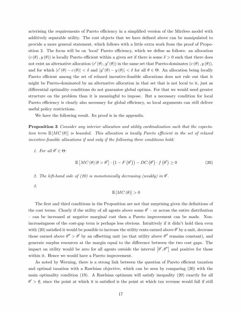
Proposition 3 Consider any interior allocation and utility cardinalisation such that the expecta-tion term E [MC (θ)] is bounded. This allocation is locally Pareto effi cient in the set of relaxed

incentive-feasible allocations if and only if the following three conditions hold:

1. For all θ′ ∈ Θ:

E[MC (θ) |θ > θ′

]·(1− F

(θ′))−DC

(θ′)· f(θ′)≥ 0 (20)

2. The left-hand side of (20) is monotonically decreasing (weakly) in θ′.

3.

E [MC (θ)] > 0

The first and third conditions in the Proposition are not that surprising given the definitions of

the cost terms. Clearly if the utility of all agents above some θ′ —or across the entire distribution

— can be increased at negative marginal cost then a Pareto improvement can be made. Non-

increasingness of the cost-gap term is perhaps less obvious. Intuitively if it didn’t hold then even

with (20) satisfied it would be possible to increase the utility rents earned above θ′ by a unit, decrease

those earned above θ′′ > θ′ by an offsetting unit (so that utility above θ′′ remains constant), and

generate surplus resources at the margin equal to the difference between the two cost gaps. The

impact on utility would be zero for all agents outside the interval[θ′, θ′′

]and positive for those

within it. Hence we would have a Pareto improvement.

As noted by Werning, there is a strong link between the question of Pareto effi cient taxation

and optimal taxation with a Rawlsian objective, which can be seen by comparing (20) with the

main optimality condition (19). A Rawlsian optimum will satisfy inequality (20) exactly for all

θ′ > θ, since the point at which it is satisfied is the point at which tax revenue would fall if still

17

more productive distortions were introduced at θ′. That is, it characterises the peak of the famous

‘Laffer curve’specific to agent θ′. Going beyond that peak implies Pareto ineffi ciency —utility for

higher types is reduced, without raising any net resources. A Rawlsian ‘maxmin’criterion treats

taxpayers above θ as revenue sources alone, and thus will seek the peak of the Laffer curve when

trading off equity and effi ciency considerations for each taxpayer above θ. More general welfare

criteria that put strictly positive weight on the utility of all agents in Θ can be expected to satisfy

the inequality strictly: this follows trivially from (19) when the second term in large brackets is

positive.

How likely is it that the Pareto criterion will be satisfied in practice? In general the non-

negativity restriction (20) will simply place an upper bound on the level of the productive distortion

that is tolerable at θ′, which in turn will depend on the deeper properties of the utility function.

Higher labour supply elasticities, for instance, are more likely to be associated with a violation

of the Pareto criterion by any given decentralised tax system. But our empirical exercise below

suggests such violations are not likely to be a feature of the US income tax system at present:

marginal tax rates are not so high as to be the ‘wrong side’of the Laffer curve.

3.3.1 Implication: the Pareto ineffi ciency of linear benefit withdrawal

More interesting is the non-increasingness in θ′ that we require of the left-hand side of the inequality.

Provided the type distribution is continuous over the relevant subset of Θ, this condition will be

violated by any piecewise-linear tax schedule T (y) that incorporates decreases in the marginal rate

at threshold income levels. Such thresholds imply a non-convex, kinked budget set, and thus induce

discrete differences in the allocations of individuals whose types are arbitrarily close to one another.

At this point the agent moves from a higher to a lower marginal tax rate, and DC(θ′)will jump

discretely downwards as a consequence, whilst the first cost term in (20) is relatively unaffected.14

Thus non-increasingness will be violated.

Decreases in piecewise-linear effective tax schedules are a common feature of benefit programmes

such as the Earned Income Tax Credit in the US and the Working Tax Credit in the UK, which

augment the salary of low income earners but ‘withdraw’the associated transfer at a fixed marginal

rate as earnings rise above a certain threshold. At the upper limit of this withdrawal phase the

effective marginal tax rate can drop substantially,15 inducing a non-convexity into the budget

set. This will generally be Pareto ineffi cient. Specifically, it should be possible to deliver a strict

14With no atoms in the type distribution the left-hand side of the inequality can be written:∫ θ

θ′MC (θ) f (θ) dθ −DC

(θ′)· f(θ′)

Since MC (θ′) is finite the derivative of the first term with respect to θ′ is always finite, and equal to −MC (θ′) f (θ′).If DC (θ′) drops by a discrete amount at θ′ the overall term must therefore increase.15For instance a single taxpayer with three or more children claiming EITC in the US in 2013 will pay an effective

marginal rate of 21.06 per cent (in addition to other obligations) on incomes between $17, 530 and $46, 227, as thetotal quantity of benefits for which he or she is eligible falls with every extra dollar earned. At this upper thresholdbenefits are fully withdrawn, and the effective marginal rate thus drops by 21.06 percentage points.

18

improvement in the welfare of a subset of the agents who presently have earnings towards (but

below) the upper end of the withdrawal band, by promising them a slightly lower marginal rate

were they to work a small quantity of extra hours. ‘Smoothing out’the kink in the tax schedule

would have the effect of incentivising higher earnings from those in the upper end of the withdrawal

band —and thus delivering higher tax revenue from them —whilst leaving all others unaffected.

Notice that this argument is very similar to the case for a zero top marginal rate when there is

a finite upper type θ. There too, if the agent with type θ is stopping work with a strictly positive

marginal rate then there can be no loss to a slight cut in any taxes paid on still higher earnings,

since these taxes are not affecting the choice of any other agent. If θ chooses to work harder she

must be strictly better off, and the extra work delivers extra revenue to the policymaker. The

argument may be repeated until the marginal rate paid on the last cent earned is zero. Indeed, it

is clear from (20) that if there is a finite upper type with strictly positive density then any Pareto

effi cient tax system will not distort the allocation of that type: DC(θ)

= 0, corresponding to a

zero marginal tax rate.

3.3.2 Corollary: recovering Pareto weights

A useful corollary of Proposition 3 is that if an allocation does not violate (local) Pareto effi ciency

then there must be a set of Pareto weights for which this allocation is optimal. More formally:

Corollary 4 Suppose an allocation satisfies the requirements for Pareto effi ciency of Proposition3. Then there exists a social welfare function W of the form:

W =

∫ΘG (θ)u (θ) dF (θ)

such that the allocation achieves a local maximum for W on the set of relaxed incentive-feasible

allocations, with the function G : Θ→ R+ satisfying:

G (θ) =G

E [MC (θ)]

{DC

(θ′) fθ (θ′)f(θ′) +

dDC(θ′)

dθ′+MC

(θ′)}

(21)

for arbitrary G > 0.

The proof of this statement follows trivially from that of Proposition 3, and is omitted. G can

be interpreted as the average Pareto weight: an obvious normalisation would be to set G = 1.

The corollary proves useful when we consider how easily existing taxes can be rationalised.

If an allocation is found to be Pareto effi cient, any case for tax reform must rest on a perceived

misalignment between the existing social preferences reflected in a tax system and appropriate

social preferences. Equation 21 provides an expression for these existing preferences. We will infer

these for a smoothed version of the 2008 US tax system in Section 5.

19

3.4 Discussion: primal and dual approaches

As noted in the introduction, the existing literature on the Mirrlees model contains a number of

insightful optimality statements, and it is instructive to consider how ours relates to them. A useful

way to understand condition (19) is as a ‘primal’characterisation of the optimum, contrasting with

the ‘dual’ approach taken by, for instance, Roberts (2000) and Saez (2001). The primal/dual

distinction here is used by analogy to the closely related literature on Ramsey taxation models —in

which second-best market allocations are found within a pre-specified set of distorted ‘competitive

equilibria with taxes’.16 The primal approach to these problems is to maximise consumer utility

directly over the set of real (consumption and leisure) allocations, subject to resource constraints

and so-called ‘implementability’ restrictions, where the latter ensure that the allocation can be

decentralised. In Mirrleesian problems the equivalent restriction is incentive compatibility. Prices

(and taxes) are then implicit in the solution; they are not treated as the objects of choice. The

dual approach, by contrast, optimises welfare by choice of market prices, given the known response

of consumers to these prices. The resulting expressions are able to exploit well-known results from

consumer theory to express optimal taxes in terms of Hicksian and Marshallian demand elasticities.

Roberts (2000) and Saez (2001) independently showed how a dual approach to the Mirrlees

model could be taken, considering perturbations to a decentralised non-linear tax system. As in

Ramsey problems, the resulting expressions can be manipulated to be written in terms of compen-

sated and uncompensated labour supply elasticities. This was the key insight of Saez (2001), and

it has proved extremely useful for empirical work: it implies optimal taxes can be calculated from

estimable elasticities. A large applied literature has emerged in response, surveyed comprehensively

by Piketty and Saez (2013). These authors follow Diamond and Saez (2011) in emphasising the

practical benefits of optimality statements that depend on estimable ‘suffi cient statistics’—notably

the behavioural elasticities that feature in dual characterisations.

A lesson we hope will be drawn from the current paper is that a primal characterisation may be

just as tractable as the dual, and thus of complementary value in drawing applied policy lessons.

Though condition (19) is novel, the primal approach more generally is dominant in the growing ‘New

Dynamic Public Finance’ literature, which considers the diffi cult problem of optimal Mirrleesian

taxation over time.17 Given the complexity of this literature, one can understand Piketty and Saez’s

comment that the primal approach “tends to generate tax structures that are highly complex and

results that are sensitive to the exact primitives of the model.” 18 But in light of the present

results this judgement seems a little rash: though we have made important structural assumptions

on preferences, particularly single crossing, we believe condition (19) gives a simple and intuitive

characterisation of the optimum. With structural (parametric) forms assumed for preferences it

can also link optimal taxes to a small number of estimable parameters, such as the Frisch elasticity

of labour supply and the elasticity of intertemporal substitution. We demonstrate this in the

16See Atkinson and Stiglitz (1980) and Ljungqvist and Sargent (2012) for useful discussions of this distinction.17See Kocherlakota (2010) and Golosov, Tsyvinski and Werning (2006) for introductions to this literature.18Piketty and Saez use the terminology ‘mechanism design approach’ in place of what is labelled the ‘primal

approach’here.

20

subsequent section. Therefore we hope that our primal method might be seen not in contrast to a

‘suffi cient statistics’approach to tax policy, but rather as contributing to it.

Whether the dual or primal characterisation will be simpler in general depends —here as in

Ramsey models —on the structure of consumer preferences. As a general rule additive separability

in the direct utility function tends to yield greater tractibility in the primal problem, as relevant

cross-derivatives of the utility function can then be set to zero. This accounts for the dominant use

of the primal approach in studying dynamic taxation problems of both Ramsey and Mirrleesian

form, where preferences are generally assumed separable across time and states of the world.19

Dual representations, by contrast, generally depend on the complete set of cross-price elasticities in

different time periods and states of the world —that is, on an intractably large Slutsky substitution

matrix. For this reason the primal approach is likely to continue to dominate the literature on

dynamic Mirrleesian problems. Indeed, Brendon (2012) shows how the main theoretical results of

the present paper can be generalised to that setting with only minor changes.

4 A parametric example

The main advantage of our approach is the tractability of condition (19) when one is willing to

impose parametric structure on individual preferences: in this case it generates simple restrictions

that can be used for empirical work. In this section we demonstrate how far the condition simpli-

fies when preferences take the isoelastic, additively separable form already discussed above. This

delivers a particularly succinct expression for the main optimality trade-off that highlights some

important consequences for optimal taxes of income effects in labour supply.

Throughout the exercise it is important to remember that the particular choice of utility function

combines a substantive statement about the structure of ordinal preferences with a normalisation

to a particular cardinal form. As discussed in section 2.2.3, the optimal allocation is invariant to

equivalent utility representations provided the social preference function G is adjusted appropri-

ately. For this reason it is advantageous to fix on a representation for which the objects MC and

DC take the simplest forms available, which will be achieved by using additively separable repre-

sentations of the direct utility function where possible —so thatMC will equal the inverse marginal

utility of consumption. For example, the set of utility functions characterised by King, Plosser and

Rebelo (1988) all describe the same ordinal consumption-labour supply preference map, and so will

deliver the same optimum with the relevant adjustment to G. It is therefore simplest to focus on

the special case of these preferences that is additively separable, with log consumption utility.20

19A good example of the former is Lucas and Stokey (1983).20 In dynamic models these arguments clearly no longer apply, as curvature in the period utility function governs

dynamic preferences.

21

4.1 Isoelastic, separable preferences

Suppose that the utility function again takes the form:

u (c, y; θ) =c1−σ − 1

1− σ −(ye−θ

)1+ 1ε

1 + 1ε

(22)

As noted above, this means thatMC (θ) collapses to the simple object c (θ)σ, whilstDC (θ) satisfies:

DC (θ) =τ (θ)

1− τ (θ)

ε

1 + εc (θ)σ

The main optimality condition (19) can then be expressed in the following form:

τ(θ′)

1− τ(θ′) =

1 + ε

ε·

1− F(θ′)

f(θ′) ·

E[c (θ)σ |θ > θ′

]− g

(θ′)E [c (θ)σ]

c(θ′)σ (23)

where we write g(θ′)as shorthand for E[Gu(u(θ))|θ>θ′]

E[Gu(u(θ))] .

This expression has dissected the term DC(θ′)in order to express taxes as a function of all

other variables, but it remains a succinct statement of the model’s key effi ciency/information-rent

trade-off. It is particularly useful for drawing attention to four distinct factors that affect this

trade-off:

1. The Frisch elasticity of labour supply: ceteris paribus a higher value for ε will result in lower

tax rates —a manifestation of the usual ‘inverse elasticity’rule.

2. The (inverse) hazard rate term 1−F (θ′)f(θ′)

: in general a lower value for this implies lower taxes.

This is the mechanical effect of giving greater weight to effi ciency costs when the distribution

of types at θ′ is dense relative to the measure of agents above that point. As an effect it was

first highlighted by Diamond (1998), and has driven much work on the shape of empirical

earnings distributions in the US and elsewhere.

3. The character of social preferences, as captured by the term g(θ′): the higher is g the lower

will be optimal taxes, reflecting the fact that reductions in information rents carry a higher

direct cost to the government the more the welfare of relatively productive agents is valued.21

4. The curvature of the utility function: for a given (increasing) consumption allocation and

given set of values for g(θ′)the final fraction is easily shown to be greater the higher is σ,

and so too will be taxes. Intuitively, more curvature in the utility function makes it more

costly to provide welfare to high types. The benefits from reducing information rents will

consequently be higher, and higher marginal taxes are desirable as a means to reduce them.

21 If G (u, θ) exhibits symmetric inequality aversion then g (θ) will range between 0 and 1, the former correspondingto a Rawlsian social objective and the latter utilitarianism.

22

The first three of these factors are well understood, but the fourth has received relatively little

attention in the literature to date. This is largely because the dual characterisation of the optimum

provided by Saez (2001) is far simpler in the case of no income effects —nested here when σ = 0.

This is no longer so acutely the case for our representation: whilst the last fraction in (23) reduces

to (1− g (θ)) under quasi-linearity, for non-zero σ it remains manageable and has an intuitive

interpretation as a measure of the relative marginal cost of providing information rents to types

above θ′.

5 Calibration results

5.1 General approach

In this section we conduct a more direct calibration exercise to assess the appropriateness of recent

US tax policy on the basis of our theoretical characterisation. Specifically, we look to place direct

numerical values on the objects in the main optimality condition (19) in order to answer the

question: How might the balance between effi ciency and equity considerations be better struck?

This exercise is based principally on consumption, earnings and tax data from the US economy in

2008, making use of the 2009 wave of the PSID data series.

We first set out the basic idea behind the empirical exercise. Recall the main optimality condi-

tion presented in Proposition 2:

f(θ′)·DC

(θ′)

(24)

=[1− F

(θ′)]·{E[MC (θ) |θ > θ′

]−E[Gu (u (θ)) |θ > θ′

]E [Gu (u (θ))]

E [MC (θ)]

}

This expression is useful because even when the equality does not hold, the objects in it can

still be interpreted as population-weighted cost terms expressing the costs of effi ciency and equity

respectively. The left-hand side is the per-capita marginal quantity of resources lost if the choices

of an agent of type θ′ are distorted in order to reduce information rents above θ′ by a unit at the

margin. The object on the right-hand side is the per-capita marginal quantity of resources gained

from this reduction in information rents, assuming that the total value of the social welfare criterion

is being held constant.

Our aim is to test how well this effi ciency-equity balance is being struck by real-world tax policy

— that is, to characterise the nature of departures from optimality. Are taxes giving insuffi cient

weight to effi ciency or to equity considerations? And how does this assessment vary as productivity

(or income) increases? In principle these questions can be answered by considering the difference

between the two cost terms in (24) for different values of θ′. To operationalise the expression we

need: (a) an individual (cardinal) preference structure, (b) a social objective, (c) a tax schedule

to test, and (d) a distribution of types. It will then be possible to infer an optimal consumption-

income choice for all types θ, and to study the properties of the (simulated) consumption-income

23

distribution that is induced across Θ. All of the objects in (24) can then be evaluated, allowing

for a direct comparison of the cost terms for each possible θ′. This in turn allows for both qualita-

tive predictions about the appropriate direction of tax reform at each given point in the earnings

distribution (of the form: ‘Insuffi cient weight is being given to effi ciency considerations for those

earning $X’), and quantitative predictions about the magnitude of gains that could be obtained

by reform. We proceed by setting out in turn the manner in which we determine the objects listed

(a) to (d) above.

5.1.1 Individual preferences

We demonstrated in section 2.2.3 that the constrained-optimal allocation is invariant as monotonically-

increasing transformations of the utility function are applied, provided the social preference function

G (·) is adjusted in a manner that compensates for this. Put differently, it is of no relevance tothe solution of the problem whether curvature in the composite function G (u (c, y; θ)) arises due

to curvature in G or in u. But clearly the overall level of curvature in this composite will have

important implications for any assessment of the effi ciency-equity balance, and for this reason it

is useful to choose a specification that clearly separates the ordinal properties of preferences from

curvature. We therefore consider the CES specification:

u (c, y; θ) =

[ωc

ε−1ε + (1− ω)

(1− ye−θ

) ε−1ε

] εε−1

(25)

where θ is again to be interpreted as the log of labour productivity, and(1− ye−θ

)corresponds

to the share of his or her time (in a year) that the agent takes as leisure. This function describes

homothetic consumption-leisure preferences by a function that is homogeneous of degree one, which

means that in a market setting with a single set of linear prices a given increase in income will

induce the same change in utility for any pair of individuals, regardless of income differences that

may exist between them. If the provision of resources to those with lower initial utility is to be

considered of greater intrinsic marginal value than provision to those with higher utility, this must

follow from curvature subsequently being applied via the function G (u). In this sense we are

normalising all curvature to derive from social preferences; but this remains a normalisation only:

optimal allocations would be unaffected if the same curvature were located in the ‘true’ utility

function.

The parameter ε is the elasticity of substitution between consumption and leisure. If ε > 1

consumption and leisure are gross complements, and if ε < 1 they are gross substitutes. In the

special case of ε = 1 the utility function limits to a Cobb-Douglas form, with exponents ω and

(1− ω) on consumption and leisure respectively. This parameterisation is consistent with the

stylised fact of no long-run labour supply effects from higher real wages, and for this reason we

consider it a benchmark case. The parameter ω gives the strength of preferences for consumption

versus leisure. Throughout what follows we calibrate it to ensure that the median income level in

our simulated income series matches that for individual workers in the US as a whole in 2008.

24

5.1.2 Social preferences

We assume that the function G (u, θ) is independent of θ, and concave in u, taking the form:

G (u; θ) =u1−γ − 1

1− γ

γ can then be interpreted as the elasticity of the marginal social value of providing resources (con-

sumption and leisure) to an individual, with respect to the quantity of resources the individual is

already consuming.22 γ = 0 corresponds to the case in which no diminishing social value accompa-

nies enrichment, whilst taking γ →∞ gives the ‘Rawlsian’limit of a max-min social objective.

5.1.3 Tax schedule

The next object that must be inputted into our analysis is an estimate for the tax schedule facing

individuals in the US in 2008. This will allow us to infer a hypothetical consumption-income

allocation induced by that schedule for any given preference structure, and that allocation in turn

can be used to gauge the balance between effi ciency and equity considerations that the estimated

tax schedule strikes. Given the complexity of the actual US tax code, as well as its variations from

state to state, we must clearly simplify substantially if we are to keep the analysis consistent with

the Mirrlees model’s assumption of a single schedule. Our approach is to estimate a non-linear,

parametric schedule linking reported 2008 income in the PSID series to the effective marginal rates

that individuals are estimated to have faced. These rates are approximated by passing detailed

income and demographic data on all primary and secondary household earners in the PSID series

through the NBER’s TAXSIM programme,23 and combining the estimated marginal income tax

rates that this generates with state-level consumption taxes to approximate the total effective

wedge at the labour-consumption margin. This gives us a series of joint observations on income

and effective marginal tax rates, to which we fit a non-linear schedule of the following form:

τ (y) = τ l + (τu − τ l)[1− (syρ + 1)

− 1ρ−1]

(26)

This is a generalisation of the schedule introduced by Gouveia and Strauss (1994), and used

widely in the quantitative public fincnace literature.24 It admits four degrees of freedom, with τ l,

τu, ρ and s to be determined. Note that y = 0 yields τ (y) = τ l and y →∞ implies τ (y)→ τu, so

these parameters can be interpreted as the lower and upper marginal tax rates respectively. ρ then

controls the degree of curvature in the marginal tax schedule, and s is a scaling parameter. We select

τ l, τu, ρ and s by minimising a sum of squared residuals between τ (y) and the estimated effective

marginal rate for each individual in the PSID series. The values we obtain are (approximately)

22The homogeneity of degree one of u helps this interpretation, as it allows the function to be read as a consumption-leisure aggregator —in the same manner as usual CES aggregators over consumption alone.23See http://www.nber.org/taxsim/24See, for instance, Conesa, Kitao and Krueger (2009) for a recent application. The standard form imposes τ l = 0

—that is, a zero marginal tax rate when incomes are zero.

25

0 0.2 0.4 0.6 0.8 1 1.2 1.4 1.6 1.8 2

x 105

­0.6

­0.4

­0.2

0

0.2

0.4

0.6

0.8

Income ($)

Mar

gina

l tax

 rate

s

DataFitted schedule

Figure 1: Estimated tax schedule

τ l = 0.13, τu = 0.42, ρ = 1.15 and s = 7× 10−6. Figure 1.charts the fitted tax schedule against the

income-marginal tax rate pairs observed in the data, for all incomes up to $200, 000. As the figure

shows, there is extremely high variance in marginal rates for low earners: this is chiefly a product

of differing eligibility for benefits programmes by demographic status —in particular, low earners

with large households to support were subject to large negative marginal rates, due to the EITC

scheme. But the average effective marginal rate at the bottom of the distribution remains positive.

The data also reveal that the highest effective marginal rates are faced by middle-income earners

—particularly those inthe EITC phase-out range. As noted above, the cut in effective marginal

tax rates that is experienced at the upper end of this phase-out range is an unambiguous source

of Pareto ineffi ciency, necessarily neglected by the smoothed schedule τ (y). This is an important

qualification to our results testing the Pareto effi ciency of τ (y) below.

We will assume that agents in the economy must choose subject to this schedule, and then

analyse the marginal effi ciency and equity costs of small changes to it. Note that the concavity

of marginal tax rates in income will imply a convex budget set in consumption-income space for

all individuals, so we may solve the model by imposing individual first-order conditions alone.

Moreover, the fact that the marginal tax schedule is continuous means that any allocations y (θ),

c (θ) that are chosen subject to it must be strictly increasing in θ. This would not be true if agents

were faced with a kinked budget set, as when marginal rates increase by a discrete amount at a

given income level. An increasing allocation ensures the validity of the first-order approach: the

allocation induced by choice subject to τ (y) will lie strictly within the set of incentive-feasible

allocations, and so small changes to it that preserve relaxed incentive-feasibility must also preserve

full incentive-feasibility.

26

Clearly this estimated schedule can only provide a first approximation to tax policy in the

US, so our focus will be on robust qualitative results that emerge for large classes of alternative

preference structures. If, for instance, we find that the marginal costs of additional ineffi ciency

outweigh the marginal costs of additional inequality for all plausible preference structures when

incomes are within a certain range, this will suggest improvements can readily be made by reducing

actual federal tax rates applicable at such incomes —particularly if actual rates exceed those of the

estimated schedule.

5.1.4 Type distribution

To obtain a distribution of types we use the joint cross-sectional earnings and expenditure data

available in the 2009 wave of the PSID (relating to 2008 tax year).25 Making use of the more detailed

expenditure data provided in recent versions of the PSID, we associate a household’s expenditure

on non-durable goods with its consumption, and use this to approximate individual (rather than

household) consumption levels by standard equivalence scales. This is then combined with the

PSID labour income data for all agents earning (and consuming) in excess of $1000, together with

an estimate of the marginal tax rate τ that the agent is likely to have faced, to infer a value for

their type under the assumption that their consumption-leisure choices satisfied the intramarginal

optimality condition:

(1− τ)ωc−1ε = (1− ω) e−θ

(1− ye−θ

)− 1ε

(27)

for a given ω and ε parameterisation. It is easy to show that this equation has a unique solution for

θ for any positive consumption-income pair. The effective marginal income tax rate faced by each

individual is approximated using TAXSIM together with state-level consumption taxes, as set out

above.26 Notice that when individuals reside in larger households condition (27) implicitly assumes

that they are nonetheless able to be the sole consumer of the goods purchased with the last dollar

that they earn at the margin.

This procedure provides us with a cross-section of values for θ particular to the chosen parame-

terisation, which we can then use to estimate the distribution of types in the 2008 US workforce

non-parametrically.27 Since we use a normal smoothing kernel the estimated distribution will not

generally be consistent with the Pareto earnings tails that Saez (2001) and Diamond and Saez

(2011) argue is a feature of US tax return data. This property can only be generated under the

present parameterisation if the type distribution has an exponential upper tail; but the upper tail

of a distribution estimated with normal kernels will never be Pareto, no matter what is the true

data generating process. To overcome this problem we calibrate the upper tail of the type distri-

bution to an exponential, with exponential parameter linked multiplicatively to α, the observed

Pareto parameter in incomes.28 We set α to 1.5, in line with the evidence provided in Diamond and25We take 2008 calendar-year data as the best available proxy for 2008 tax-year data. Full details of the data series

and estimation techniques used can be found in Appendix B.26We do not use the estimated parametric tax schedule at this stage.27We correct for sampling bias by use of the PSID population weights.28Specifically, this exponential parameter is set equal to α for ε ≥ 1, and to εα for ε < 1. These choices can easily

27

Saez (2011). The calibration is imposed only for the top 0.42 per cent of earners in the resulting

estimated distribution F (θ) —a value that is chosen to minimise discontinuities in the estimated

PDF. Despite this small range of applicability it is nonetheless significant for our results for high

earners, since it ensures the estimated value of 1 − F (θ) remains large relative to the associated

density estimate f (θ), and thus that the marginal benefits of reducing information rents continue

to be assessed at a non-negligible value even for very high types. If we were instead to use an

estimated upper tail obtained by a normal kernel it would always be optimal to let the top rate of

tax limit to zero. In this sense our results are certainly sensitive to the calibration of the upper tail

of the distribution.

For our benchmark case the individual preference parameters are set to ε = 1 and ω = 0.515.

The former (which implies Cobb-Douglas utility) is well-known to be consistent with the stylised

fact of balanced growth; more importantly for our purposes it also implies that the high-skill

individuals who have high effective wages do not on average work longer or shorter hours than their

low-skill contemporaries. As mentioned above, the value of ω is chosen so that the median income

level in the simulated series — discussed in full below — coincides with the US median personal

income level in 2008, which was approximately $26, 500.29

In Figure 2 we chart the estimated distribution of labour productivity, eθ, that corresponds to

this calibration. This has a clearer economic interpretation than θ itself: it is the annual income (in

2008 dollars) that an agent would earn if he or she were to spend no time at leisure. As one would

expect, the productivity distribution replicates well-known features of the income distribution,

notably a large degree of positive skewness.

Note finally that because we have not chosen to focus our attention on quasi-linear preferences

the inference procedure for the type distribution is more complex than it would otherwise be.

Quasi-linearity has the well-known advantage that the level of consumption does not feature in

the consumption-leisure optimality condition (27), and so θ can be inferred from earnings data

alone. This allows, in particular, for detailed government data on tax returns to be applied to the

exercise, as in Saez (2001) and many subsequent papers. For the general case this is not possible,

as tax returns do not provide corresponding information on consumption. One could proceed by

inferring post-tax income and imposing that this must equal consumption —a procedure followed,

for instance, by Blundell and Shephard (2012) in their assessment of the optimal tax treatment of

single mothers in the UK. But this does risk biasing the results. In particular it implies that agents

with very high incomes should also have very high consumption levels, and thus very low marginal

utilities of consumption. This would tend to over-state θ for high earners, for whom savings are

generally substantial. This is the main reason for our use of the PSID dataset, whose detailed

consumption data allow us to infer a model-consistent type distribution without such bias.

be shown to generate upper tails for income that are approximately Pareto, with Pareto parameter α, when the toprate of income tax is fixed.29Source: Current Population Survey.

28

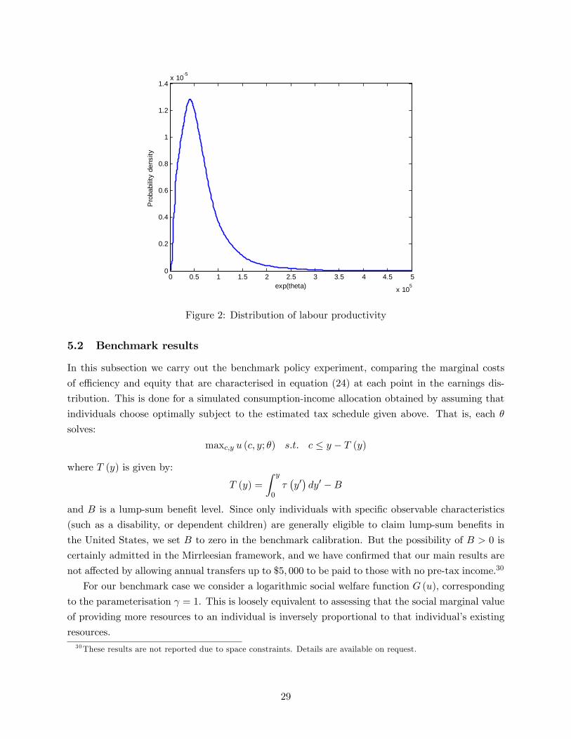
0 0.5 1 1.5 2 2.5 3 3.5 4 4.5 5

x 105

0

0.2

0.4

0.6

0.8

1

1.2

1.4x 10­5

exp(theta)

Pro

babi

lity 

dens

ity

Figure 2: Distribution of labour productivity

5.2 Benchmark results

In this subsection we carry out the benchmark policy experiment, comparing the marginal costs

of effi ciency and equity that are characterised in equation (24) at each point in the earnings dis-

tribution. This is done for a simulated consumption-income allocation obtained by assuming that

individuals choose optimally subject to the estimated tax schedule given above. That is, each θ

solves:

maxc,y u (c, y; θ) s.t. c ≤ y − T (y)

where T (y) is given by:

T (y) =

∫ y

0τ(y′)dy′ −B

and B is a lump-sum benefit level. Since only individuals with specific observable characteristics

(such as a disability, or dependent children) are generally eligible to claim lump-sum benefits in

the United States, we set B to zero in the benchmark calibration. But the possibility of B > 0 is

certainly admitted in the Mirrleesian framework, and we have confirmed that our main results are

not affected by allowing annual transfers up to $5, 000 to be paid to those with no pre-tax income.30

For our benchmark case we consider a logarithmic social welfare function G (u), corresponding

to the parameterisation γ = 1. This is loosely equivalent to assessing that the social marginal value

of providing more resources to an individual is inversely proportional to that individual’s existing

resources.30These results are not reported due to space constraints. Details are available on request.

29

5.2.1 Effi ciency-equity gap

Having simulated a consumption-income allocation across all types, we can then use this to graph

the cost difference term ∆ (θ):

∆ (θ) : =[1− F

(θ′)]·{E[MC (θ) |θ > θ′

]−E[Gu (u (θ)) |θ > θ′

]E [Gu (u (θ))]

E [MC (θ)]

}−f(θ′)·DC

(θ′)

against y (θ). This term can be understood as the marginal quantity of resources that would be

gained per worker in the economy from a tax reform that held constant the value of the social

objective but reduced information rents by a unit at θ. When it is positive the implication is that

greater focus should be given to reducing inequality in welfare relative to θ, since information rents

are more costly than a policymaker with the chosen objective criterion should be willing to tolerate.

When negative the implication is that too great a degree of productive distortion is witnessed at

θ, and more information rents above that point ought to be tolerated.

Figure 3 plots ∆ (θ) for the benchmark calibration, for incomes ranging between zero and

$500, 000. The most striking feature of the figure is the non-negativity of ∆ (θ) at all income

levels: the marginal cost of distorting production in order to reduce information rents is always less

than the marginal quantity of resources that are freed up as a consequence, holding constant the

value of the social objective. Thus the approximated tax schedule that we consider permits greater

information rents than ought to be the case for a social planner with γ = 1, across all levels of

income. By increasing the marginal distortion faced by an individual earning around $17, 500 and

redistributing the proceeds uniformly (in utility terms) across the population, the government could

—if the calibration is accurate —generate an additional $60 per taxpayer at the margin, for every

unit by which information rents above $17, 500 are reduced. To put this in context, the marginal

cost of providing a unit utility to higher types in an incentive-compatible manner is around $430

per capita,31 so in this case the result is saying that for every $430 by which the relative post-tax

resources of higher types (earning above $17, 500) is reduced, the government can retain a surplus

of $60 per capita —even after redistributing resources across the population to hold social welfare

constant. As mentioned in the introduction, this corresponds to a dollar’s surplus raised per capita

for every seven dollars by which post-tax resource inequality is reduced.

The cost gap term ∆ (θ) is maximised for relatively low income levels: $17, 500 is slightly above

the lower quartile of the simulated distribution. In itself this is an interesting result, since the focus

of policy work in the optimal tax literature often gives special treatment to the problem of finding

the optimal top rate, distinct from more general questions about the rest of the schedule.32 Yet it

is not clear that the resources to be gained from getting the top rate right are any more significant

than those available from striking a better trade-off elsewhere. The results here instead suggest

31That is, this is the value of E [MC (θ) |θ > θ′] for the corresponding θ′.32See, for instance, Chapter 2 of the first volume of the Mirrlees Review (Mirrlees, 2010).

30

0 0.5 1 1.5 2 2.5 3 3.5 4 4.5 5

x 105

­10

0

10

20

30

40

50

60

70

Pre­tax income ($)

Equ

ity c

ost ­

 Effi

cien

cy c

ost (

$)

Figure 3: Cost difference: benchmark calibration

low-to-intermediate intermediate tax bands may be of much greater consequence —offering by far

the greatest scope for marginal improvements for a policymaker with preferences of the type that

we have assumed.

But on the surface these conclusions appear contradictory. On the one hand we are finding that

tax policy is giving insuffi cient weight to equity concerns; on the other we are prescribing higher

marginal tax rates on relatively low earnings ranges as a means to address this. To account for

this we need to address the common confusion between marginal and average tax rates. Suppose

that one wishes to target redistribution at the very poorest in society — those earning less than

$17, 500, say —in a manner that is resource-neutral. The most direct means to do this is to increase

the marginal tax rate paid at $17, 500. This will reduce the post-tax resources available to all

those earning $17, 500 or more: an agent’s total tax bill is the integral of the marginal rate over

all incomes up to their own. Provided that the government then uses the associated tax revenue

to redistribute uniformly across the population, there will be a net increase in welfare for those

earning less than $17, 500, and a net reduction for those earning more. Raising marginal taxes paid

at $17, 500 is thus a way to increase average taxes for all those who earn more than this, and reduce

them for those who earn less. Our results suggest that US tax policy in 2008 was doing too little

to target post-tax resources at very low earners in this way.

5.3 Sensitivity

The strongest result above is the qualitative one, that regardless of the tax schedule considered the

marginal costs from additional ineffi ciency in agents’production decisions are always outweighed

by the marginal benefits from reducing information rents, given unit-elastic curvature in the social

31

objective criterion. In this subsection we test how sensitive these results are to alternative para-

meterisations for individual and social preferences. We consider variations along two dimensions:

changes in the elasticity of substitution between consumption and leisure, and changes in the degree

of curvature applied to utility in the social welfare objective. The last of these also provides an op-

portunity to assess the simulated distribution against the restrictions implied by Pareto effi ciency,

derived in Section 3.3 above.

5.3.1 Labour supply elasticity

We first consider the impact on our results of changing ε, the elasticity of substitution between

consumption and leisure. In general ε can be shown to relate to the Hicksian (compensated)

elasticity of labour supply with respect to the real wage, eh, according to the formula:

eh =ε

l(wc + 1

1−l

)where l is labour supply and w the real wage. Replacing l with its model counterpart ye−θ and

w with the effective wage eθ (1− τ) this can be used to infer an implicit value for the Hicksian

elasticity for each observation in the PSID data series, under the assumption that preferences take

the form specified. This is useful because the Hicksian elasticity has been the object of a large

number of empirical estimates, against which we can check the values implicity being used here. At

the benchmark calibration (ε = 1) the mean implicit value of this elasticity in the data is around

0.64, which is considerably above the value of 0.3 suggested by Chetty (2012) — itself high by

comparison with most prior estimates. The implication is ε = 1 may be too high a calibration.33

Figure 4 thus shows the effect on the cost comparison of instead reducing ε to 0.5.34 There

are two notable features of the figure. First, its qualitative form is very similar to that of the

benchmark case in Figure 3. In particular, the cost gap is highest (and positive) for low-to-middle

income earners, peaking in this case at an income of a little over $20, 000.35 Once more, the

marginal cost of permitting information rents at this point in the income distribution is far greater

than the marginal effi ciency cost of raising tax distortions, suggesting substantial unrealised gains

from reducing the relative incomes of higher earners —at least for a policymaker with the chosen

preference structure. Second, and in contrast with the benchmark case, the cost gap now turns

slightly negative for large income earners, suggesting that the estimated effective upper rate of tax,

42 per cent, is slightly higher than the optimal top rate, and a small reduction in upper tax rates

would reduce productive distortions suffi ciently to be beneficial. A possible reason for this is that

33Against this is the fact that ε = 1 is the only calibration consistent with no trend in labour supply as productivityincreases. When ε < 1 consumption and leisure are gross complements, which means that more productive agentstend to work shorter hours.34ω is simultaneously adjusted to continue to match a median income of $26, 500.35The quantitative magnitude of the cost difference is clearly smaller than in the benchmark case for all income

levels. But the main reason for this is simply that a unit of utility is itself worth less in dollar terms, so that theimplicit change in income inequality that is being considered as utility inequality is reduced by a unit is itself nowsmaller.

32

0 0.5 1 1.5 2 2.5 3 3.5 4 4.5 5

x 105

­0.2

0

0.2

0.4

0.6

0.8

1

1.2

1.4

Pre­tax income ($)

Equ

ity c

ost ­

 Effi

cien

cy c

ost (

$)

Figure 4: Cost difference: ε = 0.5

since leisure and consumption are now gross complements, the quantity of hours worked by high

types is very low. This holds down the information rents available at high earnings levels, in turn

tending to raise the cost of the marginal additional distortions needed to reduce them still further.36

We take from this exercise that the qualitative result of a significant, positive gap between

the marginal cost of inequality and the marginal cost of ineffi ciency at low incomes appears to

generalise to lower values for the elasticity of substitution between consumption and leisure. But

setting ε to 0.5 also appears to undermine the uniformity of the benchmark finding that marginal

effi ciency costs are everywhere lower than marginal equity costs: at high incomes this is no longer

true. The results from the upper tail of the income distribution here ought to be treated with some

care though: gross complementarity renders the associated labour supply of high types implausibly

low by comparison with their lower-productivity peers.

5.3.2 Social preferences

We next consider the effect on the results of changing the degree of curvature that the policymaker

applies through the parameter γ in the function G (u; θ). There are two limiting cases of interest.

First, the ‘utilitarian’assumption of no curvature: γ = 0. In this situation there is no intrinsic

inequality aversion in social preferences, in the sense that doubling an agent’s consumption and

leisure levels would not change the marginal social value of giving that agent extra consumption

(or leisure). The second limiting case is the Rawlsian scenario, in which γ → ∞ and the social

objective becomes a ‘max-min’criterion. We saw above that the shape of the cost gap assessed

36To take an extreme case, if no hours were being worked then no information rents would be available. DC wouldbe infinite in this situation.

33

in this case has important implications for the Pareto effi ciency of the allocation under arbitrary

social preference assumptions.

Utilitarian criterion One might expect that when γ = 0 is imposed ∆ (θ) should always be

negative. A diminishing marginal social value of providing resources to individuals is the main force

motivating redistribution in the Mirrlees model, and so without it the ineffi ciency costs of taxation

could be expected to dominate the marginal costs of inequality. But surprisingly this intuition turns

out not to be correct. The reason is that the consumption-leisure ratio is not constant across types.

Higher values for this ratio make it relatively more costly to provide additional utility through

consumption, even while the utility function is homogeneous of degree one overall. So long as the

vector that is associated with incentive-compatible utility provision has a large enough consumption

component, the result is that MC (θ) will tend to grow in θ. Intuitively, it remains desirable to

redistribute consumable resources to those who are consumption-poor relative to the quantity of

leisure they enjoy.

Figure 5 plots the cost comparison for the utilitarian case, using the benchmark calibration

of ε = 1. For all pre-tax incomes less than $24, 500 the gap is again positive, suggesting that

even a policymaker with no ‘intrinsic’aversion to inequality in the distribution of resources should

be willing to tolerate greater ineffi ciencies at the lower end of the US income distribution, so as

to reduce post-tax inequality. Recall that the calibration is matching a median pre-tax income

of $26, 500, so the implication is that there would be net benefits to increasing the productive

ineffi ciency of almost the entire lower half of US earners. But for incomes between $24, 500 and

$117, 000 the cost gap is now negative, with the higher marginal tax rates that this group is paying —

together with a lower value for the inverse hazard rate term 1−F (θ)f(θ) —reducing the relative marginal

benefits to additional tax distortions. The cost gap then turns positive for still higher incomes:

even without inequality aversion, under the benchmark calibration a top income tax rate of 45 per

cent is too low.

The main lesson that we take from this exercise is the surprising endurance of the incentive

to redistribute, even when this incentive is not admitted directly through curvature in the social

welfare criterion. The presence of a positive cost gap at low-to-middle incomes in particular appears

to be a very robust finding.

Rawlsian criterion and Pareto effi ciency Figure 6 plots∆ (θ) when the social welfare criterion

is assumed to be a Rawlsian ‘max-min’function, again using the benchmark calibration ε = 1. This

is equivalent to setting E[Gu(u(θ))|θ>θ′]E[Gu(u(θ))] to zero for all θ′ > θ (with θ the lowest type), so it is inevitable

that ∆ (θ) increases relative to the benchmark at all income levels.37 Hence the cost gap remains

positive for all θ: a Rawlsian policymaker simply seeks to maximise the quantity of tax revenue

raised from each type (above the lowest), and the estimated tax system systematically sets rates

too low to do this.37The simulated allocations are unaffected by social preferences.

34

0 0.5 1 1.5 2 2.5 3 3.5 4 4.5 5

x 105

­15

­10

­5

0

5

10

15

Pre­tax income ($)

Equ

ity c

ost ­

 Effi

cien

cy c

ost (

$)

Figure 5: Cost difference: utilitarian case

0 0.5 1 1.5 2 2.5 3 3.5 4 4.5 5

x 105

­50

0

50

100

150

200

250

300

350

400

Pre­tax income ($)

Equ

ity c

ost ­

 Effi

cien

cy c

ost (

$)

Figure 6: Cost difference: Rawlsian case

35

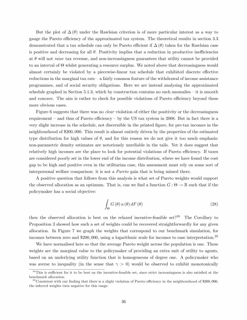
But the plot of ∆ (θ) under the Rawlsian criterion is of more particular interest as a way to

gauge the Pareto effi ciency of the approximated tax system. The theoretical results in section 3.3

demonstrated that a tax schedule can only be Pareto effi cient if ∆ (θ) taken for the Rawlsian case

is positive and decreasing for all θ. Positivity implies that a reduction in productive ineffi ciencies

at θ will not raise tax revenue, and non-increasingness guarantees that utility cannot be provided

to an interval of Θ whilst generating a resource surplus. We noted above that decreasingness would

almost certainly be violated by a piecewise-linear tax schedule that exhibited discrete effective

reductions in the marginal tax rate —a fairly common feature of the withdrawal of income assistance

programmes, and of social security obligations. Here we are instead analysing the approximated

schedule graphed in Section 5.1.3, which by construction contains no such anomalies —it is smooth

and concave. The aim is rather to check for possible violations of Pareto effi ciency beyond these

more obvious cases.

Figure 6 suggests that there was no clear violation of either the positivity or the decreasingness

requirement —and thus of Pareto effi ciency —by the US tax system in 2008. But in fact there is a

very slight increase in the schedule, not discernible in the printed figure, for pre-tax incomes in the

neighbourhood of $200, 000. This result is almost entirely driven by the properties of the estimated

type distribution for high values of θ, and for this reason we do not give it too much emphasis:

non-parametric density estimates are notoriously unreliable in the tails. Yet it does suggest that

relatively high incomes are the place to look for potential violations of Pareto effi ciency. If taxes

are considered poorly set in the lower end of the income distribution, where we have found the cost

gap to be high and positive even in the utilitarian case, this assessment must rely on some sort of

interpersonal welfare comparison: it is not a Pareto gain that is being missed there.

A positive question that follows from this analysis is what set of Pareto weights would support

the observed allocation as an optimum. That is, can we find a function G : Θ→ R such that if thepolicymaker has a social objective: ∫

ΘG (θ)u (θ) dF (θ) (28)

then the observed allocation is best on the relaxed incentive-feasible set?38 The Corollary to

Proposition 3 showed how such a set of weights could be recovered straightforwardly for any given

allocation. In Figure 7 we graph the weights that correspond to our benchmark simulation, for

incomes between zero and $200, 000, using a logarithmic scale for incomes to ease interpretation.39

We have normalised here so that the average Pareto weight across the population is one. These

weights are the marginal value to the policymaker of providing an extra unit of utility to agents,

based on an underlying utility function that is homogeneous of degree one. A policymaker who

was averse to inequality (in the sense that γ > 0) would be observed to exhibit monotonically

38This is suffi cient for it to be best on the incentive-feasible set, since strict increasingness is also satisfied at thebenchmark allocation.39Consistent with our finding that there is a slight violation of Pareto effi ciency in the neighbourhood of $200, 000,

the inferred weights turn negative for this range.

36

103 104 1050

0.2

0.4

0.6

0.8

1

1.2

1.4

Income ($, logarithmic scale)

Par

eto 

wei

ght

Medianincome

Figure 7: Pareto weights consistent with chosen allocation

decreasing Pareto weights in this context. The inferred series instead exhibits a pattern that seems

easier to account for by a political economy argument. The only agents whose (marginal) welfare

is given a weight above average —for the range graphed —are those in the neighbourhood of the

median income level —more precisely, those earning between around $14, 000 and $38, 000. This

covers roughly half the population in the simulated distribution, from the 20th to the 70th earnings

percentile. It suggests those at the extremes of the income distribution have not been as successful

in seeing their preferences reflected in acual US taxes as those closer the centre. This is entirely

consistent with our earlier analysis suggesting that even a utilitarian policymaker could gain from

raising taxes on low-to-middle income ranges: doing so is a means to target resources at the very

poorest, who earn lower still.

As with the test of Pareto effi ciency itself, the part of this result that relates to relatively high

earners is sensitive to the relatively imprecise estimation of the upper tail of the type distribution.

Indeed, if one extends the income range covered in the Figure to include types in the fitted expo-

nential tail, the associated weights grow in income without bound. Those whose types fall within

the fitted tail always have a Pareto weight in excess of one. Perhaps this result can be interpreted

as evidence that those with high incomes can rival the median voter for political influence, but since

it depends heavily on the calibrated part of the type distribution we do not wish to exaggerate its

significance.

37

6 Conclusion

Despite pioneering the genre, the Mirrleesian optimal income tax model stands strangely apart

from most other screening problems in the manner in which it is conventionally analysed. Since

the seminal work of Saez (2001) the focus of the tax literature has been on the direct role of labour

supply elasticities, social preference parameters and the structure of the type distribution in shaping

optimal rates. It has been rare to frame these objects in terms of the key trade-off emphasised by

the parallel mechanism design literature —between the competing costs of information rents and

productive effi ciency. This paper has presented a new characterisation of the Mirrlees problem that

is directly interpretable in terms of these latter objects, and explores the practical insights that it

provides.

Specifically, we defined two marginal cost variables that capture, in turn, the cost of providing

utility in a manner that keeps information rents constant, and the cost of reducing information rents

in a manner that leaves utility constant. We demonstrated that these objects must satisfy a number

of simple and intuitive relationships to one another at any optimum. Moreover, as cost terms they

can be used to analyse existing tax schedules, providing meaningful answers to central questions

such as: Does the current tax system give too much weight to effi ciency to equity considerations,

and how does this vary along the income scale? We showed how to operationalise such questions

in section 5, inferring a distribution of productivity types for the US economy based on data from

the 2009 wave of the PSID, and using this to simulate our key cost terms over the entire income

distribution, given an estimated parametric marginal tax schedule.

The results strongly implied that the US tax system is giving too little weight to equity concerns

relative to effi ciency, particularly in its treatment of low-to-middle income earners, in the sense

that the marginal costs of tolerating information rents at each point in the induced consumption-

income allocation are far greater than the marginal effi ciency costs that would have to be paid to

reduce them. This result applies uniformly across the income distribution under our benchmark

calibration, which assumes logarithmic curvature of the social welfare criterion in individual utility

levels. Surprisingly, it also applies for the lower half of the income distribution even when social

preferences are utilitarian, aggregating individual utility functions that are themselves homogeneous

of degree one in consumption and leisure —so that social preferences exhibit no ‘intrinsic’aversion

to inequality. Even then there would be gains to reducing the gap in post-tax utility levels between

low earners and those with higher productivity.

On the surface this result is contradictory. It seems to be saying that the tax system gives

insuffi cient weight to equity concerns, but that the best response to this is to tax low-to-middle

income earners more! This highlights an important confusion that can often arise in popular

discussions about income taxes, whereby the marginal tax rate an individual faces is conflated with

their average tax rate. An increase in the marginal tax rate paid on earnings in the region of,

say, $15, 000 reduces the post-tax income of all those who earn more than this income level, and

holds constant the income of all those who earn up to this income level. If the proceeds are then

redistributed uniformly across the population, for instance by providing a fixed, positive benefit

38

level that one can receive irrespective of earnings, the net beneficiaries of the combined reform are

precisely those earning less than $15, 000 originally. Higher marginal taxe rates on low-to-middle

income ranges are therefore best interpreted as a means to target redistribution to the very poorest

earners. They are the only way to reduce post-tax income dispersion among those in the lower end

of the income distribution. This is just as desirable as reducing inequality more generally under a

generalised utilitarian criterion of the sort we consider.

Our theoretical results also provide a new test of the Pareto effi ciency of any given tax sys-

tem, substantially generalising the approach of Werning (2007). When we apply this test to the

approximated 2008 tax schedule we find no clear violation of Pareto effi ciency; but ímportantly

the pattern of Pareto weights that is required for the given allocation to be optimal does not place

higher weighting on the marginal welfare of poorer agents, as would be expected of a social planner

who was averse to inequality. Instead it is those in the middle of the income distribution who

receive disproportionately high weighting, consistent with a ‘median voter’theory of tax policy. It

will be interesting to see how far this result carries through under equivalent simulations based on

different tax years and data series.

Some of these results are clearly quite contentious, and for this reason we stress that our

approach is certainly not without its limitations. The most significant of these is that we rely on

the static version of the Mirrlees model. This is important because the static model assumes the tax

system is the only means individuals have for providing themselves with consumption insurance —a

factor that may bias policy preferences in favour of more distribution than would be optimal were

precautionary savings behaviour appropriately incorporated. Note, for instance, that if incomes

had a large stochastic component then those with high earnings one year would not necessarily

consume much more than those whose earnings were substantially lower, and thus differences in

the marginal cost of providing utility to each of them might not be so substantial.

Nonetheless, it is not clear why developing the analysis in a dynamic setting should be expected

to reverse the main results on the relative merits of tax reform. So for now at least are left with a

puzzle: given the improved redistribution that such a strategy could effect, why does the US not

apply higher marginal tax rates on low-to-middle income ranges?

References

[1] Atkinson, A.B., and J.E. Stiglitz (1980), Lectures on Public Economics (Second Ed.), McGraw-

Hill.

[2] Blundell, R., and A. Shephard (2012), ‘Employment, Hours of Work and the Optimal Taxation

of Low-Income Families’, Review of Economic Studies, 79, 481—510.

[3] Brendon, C.F. (2012), ‘Effi ciency-equity Trade-offs for Dynamic Mirrleesian Tax Problems’,

Manuscript (available at http://mwpweb.eu/CharlesBrendon)

39

[4] Butrica, B.A., and R.V. Burkhauser (1997), ‘Estimating Federal Income Tax

Burdens for Panel Study of Income Dynamics (PSID) Families using the Na-

tional Bureau of Economic Research TAXSIM Model’, working paper available at:

http://www.maxwell.syr.edu/uploadedFiles/cpr/publications/aging_studies/age12.pdf

[5] Chetty, R. (2006), ‘A New Method of Estimating Risk Aversion’, American Economic Review,

96, 1821—1834.

[6] Chetty, R. (2012), ‘Bounds on Elasticities with Optimization Frictions: A Synthesis of Micro

and Macro Evidence on Labor Supply’, Econometrica, 80, 969—1018.

[7] Chetty, R., A. Guren, D. Manoli and A. Weber (2011), ‘Are Micro and Macro Labor Sup-

ply Elasticities Consistent? A Review of Evidence on the Intensive and Extensive Margins’,

American Economic Review, 101, 471—475.

[8] Conesa, J.C., S. Kitao and D. Krueger (2009), ‘Taxing Capital? Not a Bad Idea after All!’,

American Economic Review, 99, 25—48.

[9] Costa, D.L. (2000), ‘The Wage and the Length of the Work Day: From the 1890s to 1991’,

Journal of Labor Economics, 18, 156—181.

[10] Diamond, P.A. (1998), ‘Optimal Income Taxation: An Example with a U-Shaped Pattern of

Optimal Marginal Tax Rates’, American Economic Review, 88, 83—95.

[11] Diamond, P.A., and E. Saez (2011), ‘The Case for a Progressive Tax: From Basic Research to

Policy Recommendations’, Journal of Economic Perspectives, 25, 165—190.

[12] Golosov, M., N.R. Kocherlakota and A. Tsyvinski (2003), ‘Optimal Indirect and Capital Tax-

ation’, Review of Economic Studies, 70, 569—587.

[13] Golosov, M., A. Tsyvinski and I. Werning (2006), ‘The New Dynamic Public Finance: A User’s

Guide’, NBER Macroeconomics Annual, 21, 317—363.

[14] Gouveia, M., and R.P. Strauss (1994), ‘Effective Federal Tax Functions: An Exploratory

Empirical Analysis’, National Tax Journal, 47, 317—340.

[15] Greenwood, J., Z. Hercowitz and G. Huffman (1988), ‘Investment, Capacity Utilization, and

the Real Business Cycles’, American Economic Review, 78, 402—417.

[16] Jones, M.C. (1991), ‘Kernel Density Estimation for Length-Biased Data’, Biometrika, 78, 511—

519.

[17] King, R.G., C.I. Plosser and S.T. Rebelo (1988), ‘Production, Growth and Business Cycles I:

The Basic Neoclassical Model’, Journal of Monetary Economics, 21, 195—232.

[18] Kocherlakota, N.R. (2010), The New Dynamic Public Finance, Princeton, Princeton University

Press.

40

[19] Ljungqvist, L., and T.J. Sargent (2012), Recursive Macroeconomic Theory, Third Edition,

MIT Press

[20] Lucas, R.E. Jr, and N.L. Stokey (1983), ‘Optimal fiscal and Monetary Policy in an Economy

without Capital’, Journal of Monetary Economics, 12, 55—93.

[21] Mankiw, N.G., M.C. Weinzierl and D. Yagan (2009), ‘Optimal Taxation in Theory and Prac-

tice’, Journal of Economic Perspectives, 23, 147—174.

[22] Mankiw, N.G., and M.C. Weinzierl (2010), ‘The Optimal Taxation of Height: A Case Study of

Utilitarian Income Redistribution’, American Economic Journal: Economic Policy, 2, 155—76.

[23] Milgrom, P., and I. Segal (2002), ‘Envelope Theorems for Arbitrary Choice Sets’, Econometrica,

70, 583—601.

[24] Mirrlees, J.A. (1971), ‘An Exploration in the Theory of Optimal Income Taxation’, Review of

Economic Studies, 38, 175—208.

[25] Mirrlees, J.A. (ed.) (2010), Dimensions of Tax Design: The Mirrlees Review, Institute for

Fiscal Studies, Oxford University Press.

[26] Mirrlees, J.A. (ed.) (2011), Tax By Design: The Mirrlees Review, Institute for Fiscal Studies,

Oxford University Press.

[27] Piketty, T., and E. Saez (2013), ‘Optimal Labor Income Taxation’, manuscript, forthcoming

in Handbook of Public Economics, vol. 5.

[28] Piketty, T., E. Saez and S. Stantcheva (2013), ‘Optimal Taxation of Top Labor Incomes: A

Tale of Three Elasticities’, forthcoming in American Economic Journal: Economic Policy.

[29] Roberts, K. (2000), ‘A Reconsideration of the Optimal Income Tax’, in Hammond, P.J., and

G.D. Myles (eds.), Incentives and Organization: Papers in Honour of Sir James Mirrlees,

Oxford University Press.

[30] Rochet, J.-C., and Choné, P. (1998), ‘Ironing, Sweeping, and Multi-dimensional Screening’,

Econometrica, 66, 783—826.

[31] Sadka, E. (1976), ‘On Income Distribution, Incentive Effects and Optimal Income Taxation’,

Review of Economic Studies, 43, 261—268.

[32] Saez, E. (2001), ‘Using Elasticities to Derive Optimal Income Tax Rates’, Review of Economic

Studies, 68, 205—229.

[33] Saez, E. (2002), ‘Optimal Income Transfer Programs: Intensive Versus Extensive Labour Sup-

ply Responses’, Quarterly Journal of Economics, 117, 1039—1073.

41

[34] Saez, E., and S. Stantcheva (2013), ‘Generalized Social Marginal Welfare Weights for Optimal

Tax Theory’, NBER Working Paper 18835.

[35] Seade, J.K. (1977) ‘On the Shape of Optimal Tax Schedules’, Journal of Public Economics, 7,

203—236.

[36] Weinzierl, M.C. (2012), ‘Why Do We Redistribute So Much But Tag So Little? The Principle

of Equal Sacrifice and Optimal Taxation’, Harvard Business School Working Paper 12-64.

[37] Werning, I. (2007), ‘Pareto Effi cient Income Taxation’, MIT Working Paper.

A Theory appendix

A.1 Preferences and single crossing

We demonstrate here the claim in Section 2.1 that the single crossing property is implied whenever

agents have common preferences over consumption and labour supply, whilst differing in their

ability to convert labour supply into output according to θ. Specifically, suppose that preferences

over consumption and labour supply for all agents are described by a common utility function

u : R2+ → R, where u is C2, increasing in its first argument (consumption) and decreasing in its

second (labour supply), and describes normal demands for both consumption and leisure. Labour

supply, in turn, can be converted into output according to a C2 function l : R+ ×Θ→ R+. l (y; θ)

thus gives the number of hours that it takes an individual whose type is θ to produce y units of

output. We assume ly > 0, lθ < 0 and lyθ ≤ 0. The latter two restrictions imply that higher values

of θ are unambiguously associated with higher productive effi ciency. Note that this setup nests the

case in which θ is a linear productivity parameter, which means l (y; θ) = yθ .

We can then define the function u : R2+ ×Θ→ R by:

u (c, y; θ) := u (c, l (y; θ)) (29)

Given the restrictions that we have imposed on the u and l functions, the single crossing property

follows:

Lemma 5 u (c, y; θ) defined in (29) satisfies single crossing in θ. That is, for any distinct pair of

allocations (c′, y′) and (c′′, y′′) such that (c′, y′) < (c′′, y′′) (in the product order sense) and θ′ < θ′′,

if u(c′′, y′′; θ′

)≥ u

(c′y′; θ′

)then u

(c′′, y′′; θ′′

)> u

(c′y′; θ′′

).

Proof. Geometrically it is easy to see that this will be true provided the derivative condition (1) issatisfied at all allocations —that is, indifference curves in output-consumption space are uniformly

42

‘flattening’in θ. We have:

d

dθ

(−uy (c, y; θ)

uc (c, y; θ)

)= −uyθ (c, y; θ)

uc (c, y; θ)+uy (c, y; θ)

uc (c, y; θ)

ucθ (c, y; θ)

uc (c, y; θ)

= −uy (c, y; θ)

uc (c, y; θ)

[uyθ (c, y; θ)

uy (c, y; θ)− ucθ (c, y; θ)

uc (c, y; θ)

]These derivatives satisfy:

uc (c, y; θ) = uc (c, l (y; θ))

uy (c, y; θ) = ul (c, l (y; θ)) ly (y; θ)

ucθ (c, y; θ) = ucl (c, l (y; θ)) lθ (y; θ)

uyθ (c, y; θ) = ull (c, l (y; θ)) ly (y; θ) lθ (y; θ) + ul (c, l (y; θ)) lyθ (y; θ)

Plugging into the previous expression gives:

d

dθ

(−uy (c, y; θ)

uc (c, y; θ)

)= − ul (c, l (y; θ)) ly (y; θ)

uc (c, l (y; θ))

[ull (c, l (y; θ)) lθ (y; θ)

ul (c, l (y; θ))

+lyθ (y; θ)

ly (y; θ)− ucl (c, l (y; θ)) lθ (y; θ)

uc (c, l (y; θ))

]

=

>0︷ ︸︸ ︷− ul (c, l (y; θ))

uc (c, l (y; θ))

≤0

lyθ (y; θ)

>0︷ ︸︸ ︷− ul (c, l (y; θ)) ly (y; θ)

uc (c, l (y; θ))

<0

lθ (y; θ)

>0︷ ︸︸ ︷[ull (c, l (y; θ))

ul (c, l (y; θ))− ucl (c, l (y; θ))

uc (c, l (y; θ))

]where the sign of the last term follows from normality in consumption, which implies increases in

labour supply must raise the value of − uluc. This confirms condition (1), completing the proof.

A.2 Proof of Proposition 1

We first establish that an incentive-feasible allocation implies increasing c and y schedules to-

gether with condition (4). Increasingness follows almost immediately from single crossing. Sup-

pose(c(θ′), y(θ′))

>(c(θ′′), y(θ′′))for some θ′′ > θ′. θ′ must weakly prefer

(c(θ′), y(θ′))to(

c(θ′′), y(θ′′))at an incentive-feasible allocation, but then single crossing implies θ′′ must have a

strict preference for(c(θ′), y(θ′)), violating incentive compatibility.

To obtain (4), note that for all θ < θ we can find ε > 0 such that for all δ ∈ [0, ε], θ + δ ∈ Θ,

and thus by incentive compatibility we have:

u (c (θ) , y (θ) ; θ) ≥ u (c (θ + δ) , y (θ + δ) ; θ) (30)

43

and

u (c (θ + δ) , y (θ + δ) ; θ + δ) ≥ u (c (θ) , y (θ) ; θ + δ) (31)

Rearranging and taking limits we have:

limδ→0

[u (c (θ + δ) , y (θ + δ) ; θ)− u (c (θ) , y (θ) ; θ)

δ

]≤ 0 (32)

limδ→0

[u (c (θ + δ) , y (θ + δ) ; θ + δ)− u (c (θ) , y (θ) ; θ + δ)

δ

]≥ 0 (33)

But by the assumed continuity properties of u these two objects must coincide. Thus the partial

right-derivative of utility with respect to type report at an incentive-feasible allocation exists, and

is equal to zero.40 An identical argument establishes that the corresponding left-derivative exists

and is equal to zero for all θ > θ. We can summarise this by:

∂

∂σ[u (c (σ) , y (σ) ; θ)]|σ=θ = 0

Totally differentiating utility with respect to type gives:

d

dθ[u (c (θ) , y (θ) ; θ)] =

∂

∂σ[u (c (σ) , y (σ) ; θ)]|σ=θ (34)

+∂

∂θ[u (c (σ) , y (σ) ; θ)]|σ=θ

Condition (4) follows immediately.

We then need that a pair of increasing allocation schedules satisfying (4) will be globally incen-

tive compatible. Suppose otherwise. Then there must exist a pair of allocations(c(θ′), y(θ′))and(

c(θ′′), y(θ′′))for some θ′, θ′′ such that:

u(c(θ′′), y(θ′′)

; θ′)> u

(c(θ′), y(θ′)

; θ′)

Suppose first that θ′ > θ′′. We have:

u(c(θ′), y(θ′)

; θ′)

= u(c(θ′′), y(θ′′)

; θ′′)

(35)

+

∫ θ′

θ′′uθ(c(θ′′), y(θ′′)

;σ)dσ

+

∫ θ′

θ′′

d

dσ

[u(c (σ) , y (σ) ; θ′

)]dσ

= u(c(θ′′), y(θ′′)

; θ′)

(36)

+

∫ θ′

θ′′

d

dσ

[u(c (σ) , y (σ) ; θ′

)]dσ

40Notice that this does not require continuity in the allocation schedules c (·) and y (·).

44

From the envelope condition we know:

d

dσ

[u(c (σ) , y (σ) ; θ

)]∣∣∣θ=σ

= 0

Since θ′ ≥ σ for all σ in the integral in (36) it follows by single crossing that each term under the

integral must be weakly positive. But clearly this implies:

u(c(θ′), y(θ′)

; θ′)≥ u

(c(θ′′), y(θ′′)

; θ′)

contradicting the earlier supposition. A symmetric argument can be applied when θ′′ > θ′, com-

pleting the proof.

A.3 Proof of Proposition 2

An allocation that is constrained-optimal for the relaxed problem solves:

maxc(θ),y(θ)

∫θ∈Θ

G (u (θ) , θ) f (θ) dθ (37)

subject to:

u(θ′)

= u (θ) +

∫ θ′

θuθ (θ) dθ

(∀θ′ ∈ Θ

)(38)

−R ≥∫θ∈Θ

[c (θ)− y (θ)] f (θ) dθ (39)

To obtain a set of necessary conditions for this problem we construct a Lagrangian with multiplier

µ(θ′)f(θ′)dθ′ on the first constraint, and η on the second. There is a technical issue in asserting

first-order conditions when Θ has no upper support, since in this case a change to uθ (θ) affects

incentive compatibility constraints across an unbounded range of types, and the associated shadow

cost term is not guaranteed to be bounded. We first present a simple proof for the case in which

Θ has finite upper support θ, and then consider how far the arguments generalise to the case in

which θ =∞.When θ < ∞ first-order conditions with respect to c (θ) and y (θ) for θ > θ may be taken

piecewise in the usual way:41

0 = Gu(θ′)uc(θ′)f(θ′)

+ uc(θ′)µ(θ′)f(θ′)

(40)

−ucθ(θ′) ∫ θ

θ′µ (θ) f (θ) dθ − ηf

(θ′)

41Strictly these conditions need only hold F -almost everywhere on Θ in order to obtain the maximum, but thereis no loss in asserting them everywhere.

45

0 = Gu(θ′)uy(θ′)f(θ′)

+ uy(θ′)µ(θ′)f(θ′)

(41)

−uyθ(θ′) ∫ θ

θ′µ (θ) f (θ) dθ + ηf

(θ′)

Meanwhile the conditions with respect to c (θ) and y (θ) each imply:

0 =

∫θ∈Θ

µ (θ) f (θ) dθ (42)

Pre-multiplying (40) by uy(θ′)and (41) by uc

(θ′), and combining the two, gives:

η[uy(θ′)

+ uc(θ′)]f(θ′)

(43)

=[uc(θ′)uyθ(θ′)− uy

(θ′)ucθ(θ′)] ∫ θ

θ′µ (θ) f (θ) dθ

Or:

ηDC(θ′)f(θ′)

=

∫ θ

θ′µ (θ) f (θ) dθ (44)

using the definition of DC(θ′)given in the main text.

Summing (40) and (41) and rearranging gives:

(Gu(θ′)

+ µ(θ′))f(θ′)

(45)

=ucθ(θ′)

+ uyθ(θ′)

uc(θ′)

+ uy(θ′) ∫ θ

θ′µ (θ) f (θ) dθ

= ηucθ(θ′)

+ uyθ(θ′)

uc(θ′)

+ uy(θ′) DC (θ′) f (θ′)

By definition we have:ucθ(θ′)

+ uyθ(θ′)

uc(θ′)

+ uy(θ′) DC (θ′) = MC

(θ′)

(46)

so this relationship simplifies to:

Gu(θ′)

+ µ(θ′)

= ηMC(θ′)

(47)

Integrating this condition over Θ and using (42) gives an expression for η, the shadow value of

extra resources:

η =

∫θ∈ΘGu (θ) f (θ) dθ∫θ∈ΘMC (θ) f (θ) dθ

(48)

=E [Gu (θ)]

E [MC (θ)]

46

Replacing the terms in µ (θ) in the integral in (44), we have:

ηDC(θ′)f(θ′)

=

∫ θ

θ′[ηMC (θ)−Gu (θ)] f (θ) dθ (49)

Or, substituting out η:

DC(θ′)f(θ′)

=

∫ θ

θ′

[MC (θ)−Gu (θ)

E [MC (θ)]

E [Gu (θ)]

]f (θ) dθ (50)

The main expression then follows from the definition of conditional expectations.

When θ =∞ it is not immediate that the integral∫ θθ′ µ (θ) f (θ) dθ will be bounded, even though

the individual shadow cost terms µ (θ) are. Indeed it is easy to construct counter-examples in which

this is not the case at an optimal plan.42 But in any event we may still apply a calculus of variations

argument, taking first-order necessary conditions for an optimum from the Lagrangian by allowing

for carefully-constructed joint changes in c(θ′)and y

(θ′), such that information rents at θ′ are

held constant. In particular, suppose that for every unit by which c(θ′)is increased at the margin

we additionally increase y(θ′)by an amount − ucθ(θ′)

uyθ(θ′). By construction this does not affect the

incentive compatibility constraints above θ′, meaning that a necessary optimality condition can be

stated that depends only on objects specific to θ′:

0 =[Gu(θ′)

+ µ(θ′)] [

uc(θ′)−ucθ(θ′)

uyθ(θ′)uyθ (θ′)

]f(θ′)

(51)

−ηf(θ′) [

1 +ucθ(θ′)

uyθ(θ′)]

Applying the definition of MC (θ), this is easily seen to be a re-statement of (47):

Gu(θ′)

+ µ(θ′)

= ηMC(θ′)

(52)

It follows that the object∫ θθ′ µ (θ) f (θ) dθ will be bounded whenever

∫ θθ′ [Gu (θ)− ηMC (θ)] f (θ) dθ

is likewise. When this is true (by assumption), our earlier arguments can be applied to establish

the optimality condition.

A.4 Proof of Proposition 3

An allocation is Pareto effi cient in the set of relaxed incentive-feasible allocations if every alter-

native allocation within that set features at least one individual who is made strictly worse off.

Equivalently, if one fixes the cardinal structure of utility then an allocation is Pareto effi cient if

for every alternative relaxed incentive-feasible allocation there exists a set of fixed Pareto weights

42 In particular, cases exist in which the multiplier integral is bounded under one cardinalisation of the utilityfunction and social welfare objective, but under not other, equivalent representations of the problem. Details areavailable on request.

47

Gu (θ) ≥ 0 such that a policymaker assessing social welfare according to the integral:

W =

∫θ∈Θ

Gu (θ)u (θ) f (θ) dθ (53)

prefers the original allocation to the alternative.43

We consider ‘only if’first. Suppose that an allocation is Pareto effi cient. We must demonstrate

that the three conditions in the Proposition must be true. We start with the third. Suppose this is

not true: then a marginal change to the allocation that raises the utility of all agents by a unit at

the margin, holding uθ (θ) constant for all θ, must raise surplus resources. This is clearly a Pareto

improvement.

Now consider the first condition. From the proof of Proposition 2 we know that if the following

inequality holds:

DC(θ′)f(θ′)>

∫ θ

θ′

[MC (θ)− E [MC (θ)]

E [Gu (θ)]Gu (θ)

]f (θ) dθ (54)

then it must be possible for the policymaker with (marginal) Pareto weights Gu (θ) to improve on

the given allocation —generating the same value for social welfare with fewer resources. Specifically,

this can be done by reducing uθ(θ′)at the margin and increasing the relative utility of all agents

above θ′, adjusting the total quantity of resources used as required in order to hold social welfare

constant.44 Now, suppose (contrary to the Proposition) that the following is true:

∫ θ

θ′MC (θ) f (θ) dθ −DC

(θ′)f(θ′)< 0 (55)

Then, irrespective of the Pareto weights applied, we have:

DC(θ′)f(θ′)−∫ θ

θ′

[MC (θ)− E [MC (θ)]

E [Gu (θ)]Gu (θ)

]f (θ) dθ (56)

> DC(θ′)f(θ′)−∫ θ

θ′MC (θ) f (θ) dθ

> 0

This means that for any set of Pareto weights, the policymaker will benefit from a marginal re-

duction in the utility rents at θ′. Hence a policy that reduces these rents at the margin must be a

Pareto improvement.45

43That is, we have here set G (u, θ) = Gu (θ) · u for all θ ∈ Θ. The subscript on Gu (θ) is retained simply to makecomparison with the previous proof direct.44This is the function of the second term in the integral.45Alternatively, a unit reduction in uθ (θ′) and a unit increase in u (θ) for all θ > θ′ must itself generate surplus

resources at the margin, even before a further adjustment is made to keep social welfare constant. This furtheradjustment always generates further resources, since the net effect of the perturbation without it is just to raiseutility for a subset of Θ.

48

A similar argument follows by taking first differences. We know that if:

DC(θ′)f(θ′)−DC

(θ′′)f(θ′′)

(57)

>

∫ θ′′

θ′

[MC (θ)− E [MC (θ)]

E [Gu (θ)]Gu (θ)

]f (θ) dθ

holds then the policymaker with Pareto weights Gu (θ) can make an improvement by raising uθ(θ′)

(generating DC(θ′)f(θ′)resources at the margin), reducing uθ

(θ′′)(at cost DC

(θ′′)f(θ′′)), and

raising the relative utility of all agents between θ′ and θ′′ by a unit at the margin. The cost of

doing this is lower than the shadow cost of the resources it consumes. Now suppose that:

∫ θ

θ′MC (θ) f (θ) dθ −DC

(θ′)f(θ′)

is increasing in θ′ over some interval I ⊂ Θ. Then pick θ′, θ′′ ∈ I, with θ′′ > θ′. Clearly we have:

DC(θ′)f(θ′)−DC

(θ′′)f(θ′′)−∫ θ′′

θ′MC (θ) f (θ) dθ < 0 (58)

As before, this will imply

DC(θ′)f(θ′)−DC

(θ′′)f(θ′′)

(59)

>

∫ θ′′

θ′

[MC (θ)− E [MC (θ)]

E [Gu (θ)]Gu (θ)

]f (θ) dθ

is true for all possible sets of Pareto weights; the allocation cannot be Pareto effi cient.

Now we take the ‘if’part. Given an allocation such that the three conditions of the Proposition

are true, it is suffi cient to show that a set of strictly positive Pareto weights exists for which a

marginal change in allocations does not deliver an improvement. Since optimal choice is clearly

invariant to changes in the scale of these weights, we can normalise E [Gu (θ)] to 1 and focus on

finding a set of values for Gu (θ) such that the necessary conditions for a local optimum are satisfied

when these Gu (θ) values are the Pareto weights. From Proposition 2 this requires that we can find

a function Gu : Θ→ R+ that satisfies, for all θ′ ∈ Θ:

∫ θ

θ′MC (θ) f (θ) dθ −DC

(θ′)f(θ′)

= E [MC (θ)]

∫ θ

θ′Gu (θ) f (θ) dθ (60)

Since E [MC (θ)] > 0 this is clearly possible whenever the left-hand side is positive decreasing.46

46The integral on the left-hand side is clearly continuous in θ′ for all atomless type distributions, since MC (θ′) isfinite for any (finite) allocation. But it is possible that we may have discrete increases in DC (θ′) f (θ′), in which casethe integral on the right-hand side will need to be discontinuous in θ′ at corresponding points. This requires a slightgeneralisation of the notation, but can be admitted without diffi culties. Note that

∫ θ′θGu (θ) f (θ) dθ is a standard cdf

on Θ, summarising the relative weight placed by the policymaker on the marginal welfare of individuals up to θ′. Aswritten this measure does not admit atoms. If we replace it with a general measure z (θ) that does, discontinuitiesare perfectly admissible via such atoms. This corresponds to the case in which the policymaker has special concern

49

B Empirical appendix

We use this appendix to present a more detailed account of the estimation procedure for the type

density applied in section 5.

B.1 Data

Our main data source in inferring both the distribution of productivity types and the approximate

US tax schedule in 2008 is the 2009 wave of the PSID, which contains detailed individual income and

household consumption data from 8690 households relating to the 2008 calendar year. For each head

of household and spouse (where present, as defined by PSID) we construct a labour income series

as the sum of the individual’s reported non-business (variable ER46829) and business (ER46808)

labour incomes. These data are then identified with the model variable y for each individual.

We identify household-level consumption with expenditure on non-durable goods over the year,

divided into the following categories: food, utilities, transport, clothing, trips and vacations, and

other recreation. The following table lists the precise PSID series included in each category.

Category Data series

Food Food at home (ER42712,

ER42722), delivered food

(ER42716, ER42726),

food eaten out (ER42719,

ER42729)

Utilities Heating (ER42112), electric-

ity/gas (ER42114, ER42116),

water (ER42118), tele-

phone/internet (ER42120),

other utilities (ER42124)

Transport Petrol (ER42808), park-

ing (ER42809), bus/train

(ER42810), cabs (ER42811),

other (ER42812)

Clothing ER42827, ER42829

Trips & vacations ER42832, ER42834

Other recreation ER42837, ER42839

The durable consumption levels thus obtained at the household level are then converted into

individual consumption values by dividing by an ‘equivalence scale’. We use the scale applied by

Eurostat for this purpose, which assigns a value of 1 to the household head, 0.5 to any additional

for a zero-measure subset of the population, so that the Pareto weight attached to this subset is non-zero relative tothe population aggregate.

50

adults, and 0.3 to each child. Thus a family of two adults and two children will have an equivalence

scale of 2.1. The individual-level consumption data obtained in this way are identified with the

model variable c.

Our aim is to infer a series for θ based on the individual optimality condition (27), given the

series for c and y. For this we further need data on effective marginal tax rates for each individual in

the sample. Of relevance to us is the overall tax wedge that the individual faces, τ , which satisfies:

1− τ =1− τm1 + t

where (1− τm) is the rate at which disposable income increases in pre-tax income (allowing for the

effects of tax credits and social security contributions), and t is the sales tax rate. Estimated values

for τm are obtained using the NBER’s TAXSIM programme,47 given PSID data on pre-tax income

(labour and non-labour), age, marital status and other variables of relevance to tax liabilities.48

Values for t are given by the sum of state-level sales taxes and the average value of local taxes on

a state-by-state basis, for each of the 50 states plus DC. Both come from publicly available data

published by the Tax Policy Centre.49 Each individual is then assumed to face the sales tax of

their state of residence.

Together these steps give us 13,412 individual-level observations on c, y and (with the exception

of overseas territories residents) τ . We then discard entries for which either income or consumption

is less than $1000, as well as all observations from US overseas territories (for which we have

no marginal tax rate data). The income cut-off is motivated by the fact that our type-inference

procedure is based on the individual striking an optimal intensive-margin trade-off. Individuals

who earn little or no income are better characterised as being at a corner solution in their labour-

consumption choice problem. The income cut-off results in 3087 observations being dropped. There

are far fewer below the $1000 consumption threshold: 152 individuals in total. Many of these are

also below the income threshold. We motivate this threshold on the grounds of possible mis-

reporting or other anomalies: 42 of the observations dropped because of it have c = 0.

We are left with 10,250 observations from which to infer types. This is done by solving optimality

condition (27) numerically for θ at each observation, given c, y, τ and a set of parameter values.50

This gives us a set of θ values, from which we wish to obtain an estimate of the population

distribution.

B.2 Inferring a type distribution

Based on the θ series we estimate a type distribution non-parametrically, using a normal smoothing

kernel and a bandwidth that is optimised (minimising integrated mean squared error) for a Gaussian

47See http://users.nber.org/~taxsim/.48The procedure used follows standard practice for obtaining TAXSIM estimates based on PSID data, as docu-

mented in Butrica and Burkhauser (1997). Full details available on request.49See www.taxpolicycenter.org/taxfacts/Content/PDF/state_sales_tax.pdf.50 In the Cobb-Douglas case (ε = 1) it is possible to solve explicitly for θ. This speeds up the procedure considerably.

51

data-generating process. To correct for sampling bias we weight observations using the individual

weights provided by the PSID (variable ER34046), integrating these into the estimator following

a procedure set out in Jones (1991). As mentioned in the main text, the estimated distribution

obtained by this procedure will generally be unable to reproduce the stylised fact of Pareto tails

in the observed income distribution: with a finite quantity of data the tails are generally poorly

estimated, particularly outside of the observed data range.51 For this reason we replace the upper

q per cent of the estimated distribution with an exponential distribution, where q is chosen endoge-

nously to minimise discontinuities in the composite pdf that results. The exponential parameter

for this distribution is set to α when ε ≥ 1, and εα when ε < 1, where α is the Pareto parameter

in observed income data that we wish to match and ε is the elasticity of substitution between

consumption and leisure. It can be shown that these choices generate pre-tax income distributions

that are approximately Pareto in the upper tails, with Pareto parameter α, whenever the upper

rate of income tax is a constant and consumption is approximately equal to disposable income for

high earners. The calibrated, parametric specification for the upper tail is useful in subsequent

calculations, as it allows us to obtain an (approximate) analytical expression for E[MC (θ) |θ > θ′

]in the simulated series when θ′ is large. This limits the need to construct numerical approximations

to expectation terms based on probabilities in the upper tails of the type distribution.

51More specifically, it is impossible for a density estimated using normal kernels on a finite quantity of data everto have an exponential upper tail, since the tails are given by weighted sums of normal density functions.

52