The Efficiency Cost of Child Tax Benefits

Kevin J. Mumford

Purdue University

November 2008

Abstract

Child tax benefits in the U.S. federal income tax are estimated at $160 billion for 2008.

This paper examines the efficiency implications of child tax benefits in a model with

endogenous fertility. In the model, the efficiency of a chosen tax policy depends on

three key parameters that account for the responsiveness of labor supply to the income

tax rate, the responsiveness of fertility to the child subsidy level, and the cross-price

substitution effect between leisure and children. This paper uses data from the National

Longitudinal Survey of Youth (NLSY) to estimate the cross-price substitution effect

because no estimates of this parameter exist in the applied literature. The resulting

estimate implies that a tax on children rather than a child subsidy would be optimal.

This implies that the annual cost of child tax benefits, when one accounts for efficency

costs, is in the $190 to $200 billion range.

Contact Information: Department of Economics, Purdue University, 100 S. Grant Street, West Lafayette,IN 47907-2076. Email: mumford@purdue.edu

Acknowledgments: I thank Ken Arrow, Michael Boskin, Raj Chetty, Gopi Shah Goda, Louis Kaplow, ColleenManchester, Anita Pena, John Shoven, and seminar participants at Brown, BYU, Louisville, Laval, Purdue,Stanford, and the NBER Summer Institute for helpful comments. I gratefully acknowledge financial supportfrom the Kapnick Fellowship provided through the Stanford Institute for Economic Policy Research (SIEPR).An earlier draft of this paper circulated as SIEPR Discussion Paper No. 06-20.

1

1 Introduction

Families with children receive preferential treatment in the U.S. federal income tax. The

budgetary cost of these child tax benefits was about $140 billion in 2006, or about $1,900

per child.1 This is larger than the tax expenditure from the deductibility of mortgage interest

for owner-occupied homes, larger than the tax expenditure from the deductibility of state

and local taxes (including property taxes), and even larger than the tax expenditure from

the exclusion of employer contributions to medical insurance premiums. The $300 per child

subsidy in the 2008 tax rebate stimulus package is estimated to increase the budgetary cost

of child tax benefits by about $20 billion. As shown in Table 1, the real value of child tax

benefits approximately doubled over the past decade and a half due to the expansion of

existing tax provisions and the creation of new provisions.

Table 1: Estimated Budgetary Cost of Child Tax Benefits(billions of dollars)

1992 1996 1999 2004 2006

Dependent Exemption 24.1 30.7 35.8 36.4 35.9Earned Income Credit 13.0 28.2 31.3 38.0 40.2Child Tax Credit – – 19.9 31.2∗ 56.2Child Care Expenses 3.4 3.4 3.1 3.6 3.9Head of Household Status 3.0 3.5 3.7 3.9 4.1

TOTAL 43.5 65.8 93.8 113.1 140.3

Number of Children (millions) 66.5 70.2 71.9 73.3 73.7Expenditure per Child $654 $937 $1,305 $1,543 $1,904Real Expenditure per Child $940 $1,204 $1,579 $1,647 $1,904

* does not include the early child tax credit payments made in 2003

Sources: OMB analytical perspectives tables 5-1 and 19-1 various years, IRS statistics of incomepublications 1304, U.S. Census Bureau Table CH-1 (2007) Living Arrangements of Children Under

18 Years Old, and author’s calculations.

The 2008 estimated cost of $160 billion is a direct measure of the value of tax revenue

1The budgetary cost of child tax benefits is the government expenditure on refundable child tax benefitscombined with the tax expenditure of child tax benefits. The tax expenditure for a tax policy is a measureof the loss of government revenue due to the policy.

2

not received and payment made to families with children due to child tax benefit provisions.

However, a measure of the true cost of providing child tax benefits should also incorporate

economic efficiency considerations. Understanding the efficiency implications of child tax

benefits is the focus of this paper. The optimal tax results are derived using a representative

agent model where the agent decides how much time to spend working and how many children

to have. The main result is then shown to hold in a model with heterogeneous agents and

a nonlinear income tax. An extension to the model allowing for heterogeneity in the cost of

raising children (through time costs) is also considered.

The three key parameters in the model are the responsiveness of labor supply to the

income tax rate, the responsiveness of fertility to the child subsidy level, and the cross-

price substitution effect between leisure and children. There are many estimates of the labor

supply elasticity, and a few estimates of the fertility elasticity, but to my knowledge there are

no estimates of the cross-price elasticity for leisure and children. I use data from the National

Longitudinal Survey of Youth (NLSY) to estimate this cross-price elasticity. The resulting

estimate implies that a tax on children rather than a child subsidy would be optimal.

This result should not be interpreted to mean that it is optimal to tax parents for the

number of children that they have. The result is derived in a model that abstracts away

from the benefits of providing child subsidies. I only consider the efficiency implications of

providing child tax benefits and shows that when one considers the distortions associated

with child subsidies, the cost is even larger than the reported budgetary cost.2

2The term budgetary cost is more appropriate that tax expenditure here for two reasons. The first is thata large fraction of child tax benefits come through refundable credits (EITC and Child Tax Credit), thus forrecipients who have no tax liability, child tax benefits are cash payments. Second, the personal exemptionis not usually included as a tax expenditure, but is instead thought of as part of the normal tax.

3

2 Model

Models with children can be very complicated. I make a strong attempt to keep this model

simple. A more complicated extension is considered in the appendix, however, one assump-

tion that is maintained throughout the paper is that parents, to a large extent, determine

the number of children in their family. Therefore, government subsidization of children may

distort fertility choices. In this paper, agents choose how many children to have, they gain

utility from their children, and they bear the cost of raising those children.

Another important assumption is that the preferences of families can be represented by a

single utility function. The number of children enters that utility function, but the model is

static, so children do not grow up and become adults with their own utility functions. This

assumption allows us to avoid the debate on whether social welfare should be normalized to

population size, but it also means that in the model the welfare of children is only considered

through its impact on family utility.3 This assumption seems most reasonable if we consider

families with young children where each child’s utility is fully incorporated into the parent’s

utility due to parental altruism.

2.1 Representative Agent Model

Consider a simple representative agent model in a Ramsey setting where the agent chooses

how much time to spend working and the number of children to have. Social welfare in this

model is represented by the following utility function

U(C,L,N) (1)

where L is leisure (time endowment less market work time), N is the number of children,

and C is the consumption of other goods. In this specification of the model, raising children

3Kaplow (2008b) contains an excellent discussion of how to compare social welfare between populationsof different sizes in chapter 14.

4

does not require time, only money. Or alternatively, time spent raising children is considered

leisure time by the parents. By assumption, each argument of the utility function is a good,

meaning that children are a net source of enjoyment to their parents. The government has

the ability to impose a linear income tax and can either subsidize or tax children, but must

raise revenue R. There are no lump-sum taxes or subsidies and consumption is untaxed.4

In this model it is possible to derive conditions under which is it optimal to subsidize,

rather than tax, the presence of children in a family. The optimal tax policy is the policy

that is most efficient at raising the required government revenue. As will be shown, the

optimal tax treatment of children in this simple model primarily depends on the cross-price

substitution effect between leisure and children.

The efficiency cost of a tax policy is measured by its excess burden, that is, the loss of

utility greater than would have occurred had the tax revenue been collected as a lump sum

(Rosen, 1978).5 In other words, the excess burden of a tax policy is the loss in social welfare

due to the distortion in relative prices only and not that which is due to the tax-induced loss of

income. Exact measures of excess burden are defined by Diamond and McFadden (1974) and

Auerbach and Rosen (1980). However it is necessary to have an explicitly-specified utility

function in order to calculate the exact excess burden. Rather than assume a particular

utility function, we will use the well-known approximation developed by Hotelling (1938),

Hicks (1939), and Harberger (1964):

EB = −1

2

N∑

i=1

N∑

j=1

titjSij (2)

where ti is the tax rate on good i and Sij is the substitution effect for good i given an increase

4The price of consumption is the numeraire. This model with a linear income tax is equivalent to a modelwith a consumption tax and no income tax. One can either think of an income tax that decreases the priceof leisure relative to the price of consumption, or a consumption tax that increases the price of consumptionrelative to the price of leisure. The tax or subsidy of children is simply disproportionate taxation of childrenrelative to consumption goods.

5Auerbach (1985) provides a comprehensive mathematical and graphical descriptions of the excess burdenand its relation to optimal tax theory.

5

in the price of good j.

Corlett and Hague (1954) were the first to examine the excess burden of a tax policy.

Following their framework, the optimal tax policy is the one that minimizes the Hotelling-

Hicks-Harberger approximation of excess burden while raising the required government rev-

enue R.6 Assuming that the prices of all goods are constant in the relevant range and that

there are no distortions in the economy (other than those caused by taxation), the excess

burden of a tax policy is approximated by the following expression:

EB = −1

2(∆PC∆Cc + ∆PL∆Lc + ∆PN∆N c) (3)

where PC , PL, and PN are the prices and Cc, Lc, N c are the compensated demands. The

excess burden is simply the sum of the three compensated deadweight loss triangles for

consumption, leisure, and children. By assumption the only price distortions in the economy

are those caused by the tax policy.7 Consumption is untaxed (see footnote 4), thus the

change in the price of consumption is always zero. This enables us to drop the first of the

three compensated deadweight loss triangles in the expression. The remaining compensated

demands for leisure and children are both potentially affected by changes in either price:

EB = −1

2

[

∆PL

(

∂Lc

∂PL

∆PL +∂Lc

∂PN

∆PN

)

+ ∆PN

(

∂N c

∂PN

∆PN +∂N c

∂PL

∆PL

)]

. (4)

If the compensated demand curves are highly linear, equation (4) will be a close approxi-

mation of the true excess burden of the tax policy.8 Once again using the assumption that

the only distortions in the economy are those caused by the tax policy, the price change for

6One particularly important application using a similar 3-good representative agent model is Boskin andSheshinski (1983). Their application was the optimal tax treatment of the labor supply for married coupleswhere the three goods are consumption, the leisure of the husband, and the leisure of the wife. I this paper,I follow the Boskin and Sheshinski terminology.

7All goods are produced under constant returns by competitive firms employing labor as the only input,so there are no profits.

8Green and Sheshinski (1979) show when this method provides an accurate approximation (even for largetax changes) and derive an approximation built from a higher order Taylor series expansion.

6

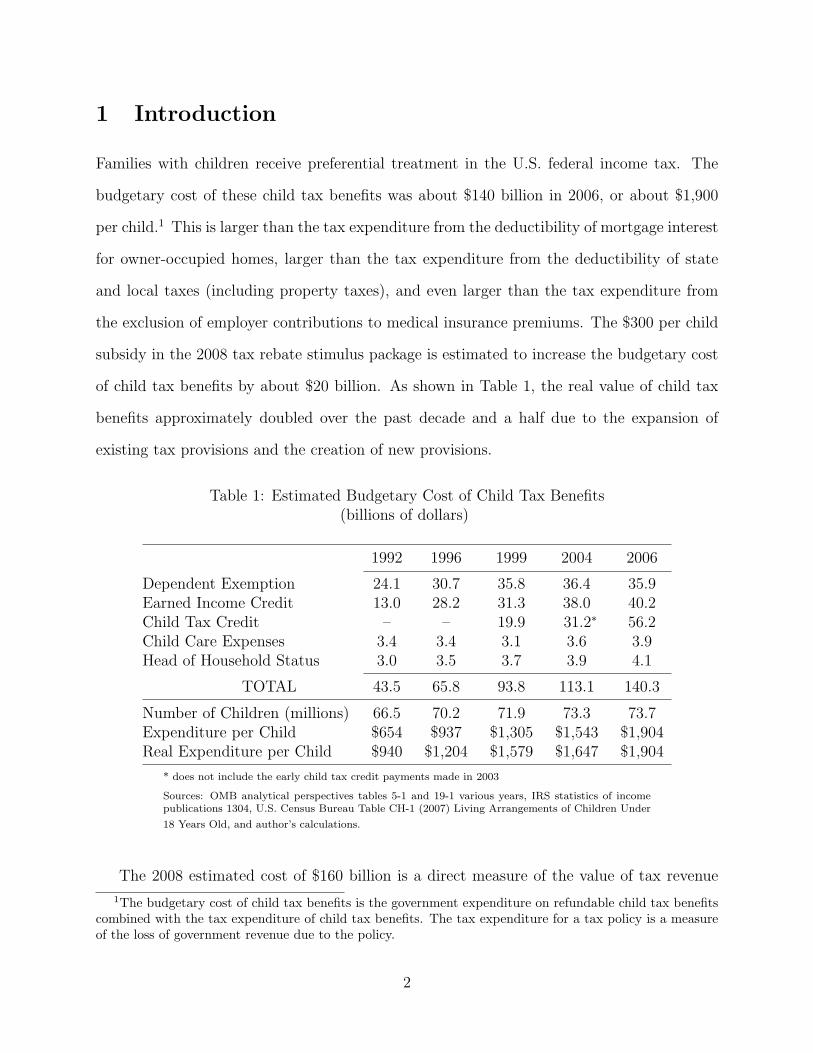
leisure is given by ∆PL = (1− τ)PL −PL = −τPL, where τ is the income tax rate. Similarly

for children, ∆PN = (1 + θ)PN − PN = θPN , where θ defines the tax treatment of children.

A positive value of θ is a tax on children whereas a negative value of θ is a child subsidy.

While it is natural to think of the price of leisure as the after-tax wage, it is less clear

what is meant by the price of children. We will take PN to represent the level of expenditure

necessary to raise a child. By assumption, the agent cannot chose to spend less than PN

for each child and any child-related expenditure above the necessary level will be considered

consumption.9

The agent has an endowment of time, T , that can be taken as leisure L, or market work,

H. The assumption that T − H = L is less restrictive than it first appears because T can

be defined to exclude time required for household and personal maintenance including sleep.

However, we are assuming that T is given exogenously and does not depend on the number

of children. This must be taken to mean that the agent considers time spent raising children

as leisure.10

Returning to the approximation of excess burden, the symmetry of the Slutsky matrix

allows (4) to be rewritten as:

EB = −1

2

(

(−τPL)2 SLL + (θPN)2 SNN + 2 SLN (−τPL) (θPN))

(5)

where S represents the substitution effect. SLN is the change in the compensated demand

for good L due to a one unit change in the price of good N . For analytical convenience,

we will scale the units of each good so that prices are unity. This means that consumption,

9This assumption can be relaxed by adding a fourth good, child quality, to the model. The main result ofthis paper (Result 2.1) still holds if the number of children and the quality of children (additional expenditureon children) are substitutes and leisure time and expenditure on children are also substitutes.

10An extension of this model that allows for a time cost of raising children is considered in the appendix.The main result of this paper (Result 2.1) still holds in the representative agent setting. However, as isshow in the numerical simulation in Section 4, adding time costs to a model with heterogeneous agents anda nonlinear income tax can produce very different results because time costs have a strong influence on themarginal utility of consumption.

7

leisure, and children are all expressed in dollar terms. For example, two children implies a

value for N of 2PN . This normalization allows us to express the agent’s “full income” budget

constraint as:

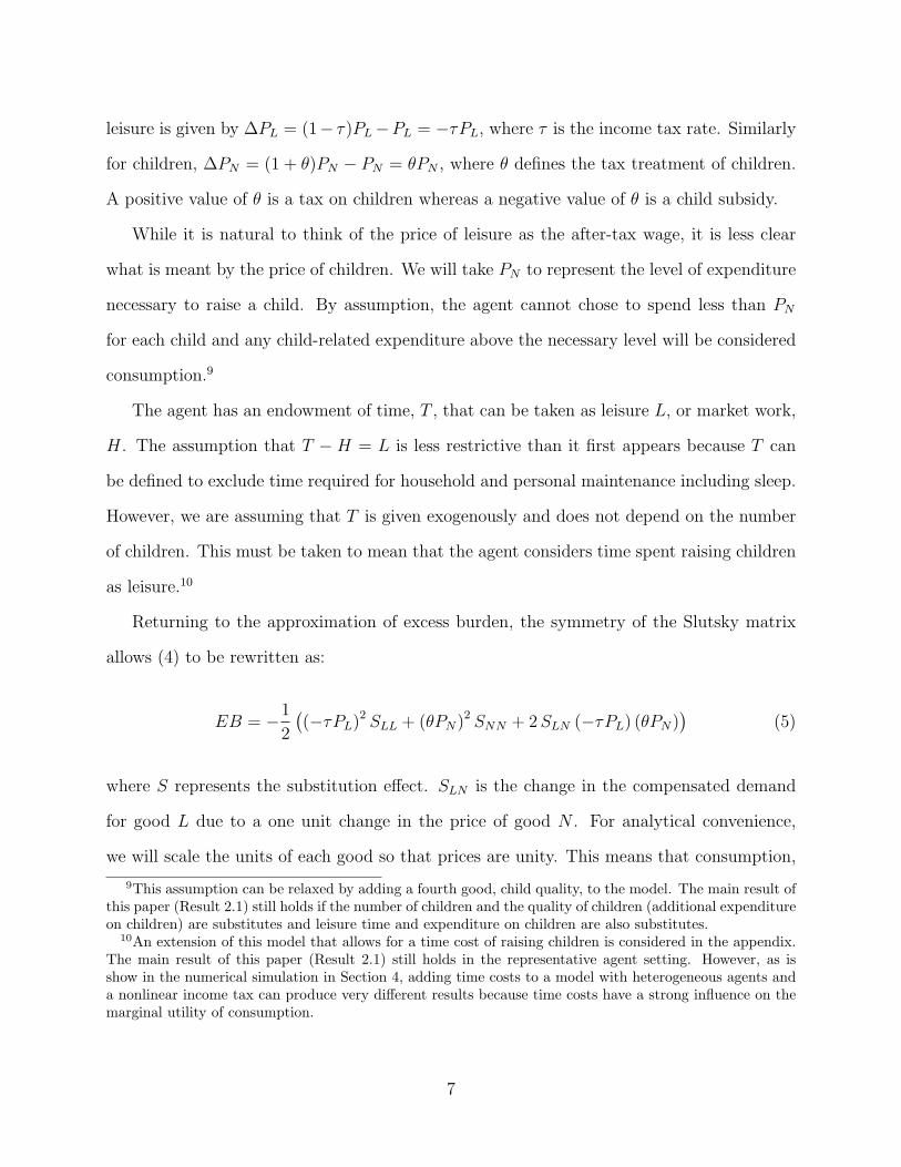
T (1 − τ) = C + L(1 − τ) + N(1 + θ). (6)

The optimal tax policy is the one that minimizes the excess burden of the tax policy

subject to raising government revenue R:

minτ, θ

{

−1

2

[

τ 2SLL + θ2SNN − 2 τθSLN

]

− λ [ τH + θN − R]

}

. (7)

The first order conditions with respect to τ and θ can be solved to yield:

τ =−λ (SNNH + SLNN)

SNNSLL − (SLN)2(8)

θ =−λ (SLLN + SLNH)

SNNSLL − (SLN)2(9)

where λ is the multiplier on the government budget constraint. The denominator for either

expression is non-negative because it is the determinant of a second-order principal minor

of the Slutsky matrix which is negative semidefinite. The multiplier λ is positive because

the excess burden of a tax policy increases in the revenue requirement, R.11 Determining

whether it is optimal to subsidize or tax the presence of children in a family is then reduced

to signing the following expression:

SLLN + SLNH. (10)

11The optimal tax policy as a function of the required government revenue, R, is given by the following:

τ =R (SLNN + SNNH)

SNNH2 + 2SLNHN + SLLN2θ =

R (SLLN + SLNH)

SNNH2 + 2SLNHN + SLLN2.

These expressions are used later in the chapter as part of a back of the envelope calculation of the optimaltax treatment of children.

8

A child subsidy is optimal if and only if SLLN + SLNH > 0. Both N and H are constrained

to be non-negative and SLL is non-positive by definition, so it is the value of SLN that is

key in determining if a child subsidy is optimal.12 A necessary condition for the optimal tax

policy to include a child subsidy is that children and leisure be substitutes.

Result 2.1. If leisure and children are complements (SLN < 0) then it is not optimal to

subsidize children.

An intuitive explanation for this result comes from considering how the compensated

demand for each good is affected by the tax policy. By totally differentiating the first order

conditions from the optimal tax problem, we can derive how the agent’s demand for leisure

and children are affected by τ and θ:

∂L

∂τ= −SLL − HiL

∂L

∂θ= SLN − NiL

∂N

∂τ= −SLN − HiN

∂N

∂θ= SNN − NiN .

The income effects, iL and iN , are not relevant in the excess burden measure because the

same level of tax revenue, R, is raised under any policy considered. If leisure and children are

complements (SLN < 0) then an increase in τ increases the compensated demand for both

leisure and children whereas an increase in θ decreases the compensated demand for both

leisure and children. The income tax distortions are reduced by imposing a tax on children

(θ > 0) because it pushes the compensated demands back in the opposite direction. A tax

on children also raises revenue, enabling the government to raise R with a lower income tax

rate.

If leisure and children are substitutes (SLN > 0), an increase in τ increases the compen-

sated demand for leisure but decreases the compensated demand for children. The income

12However, SLN , the cross-price substitution effect for leisure and children, is the only parameter of thismodel for which empirical estimates do not exists. Section 3 will turn to the task of estimating this parameter.

9

tax distortions are reduced by giving a child subsidy (θ < 0). Providing child tax benefits

is costly in that τ must be increased in order to finance the benefits, so only when leisure

and children are strong substitutes as defined by Result 2.2 is it optimal to provide child tax

benefits.

Result 2.2. If SLN > −SLL

(

NH

)

then it is optimal to subsidize children.

From this we see that subsidizing children is more likely to be optimal if there is a low

demand for children and a high supply of labor. In fact, if work effort, H, is zero then

regardless of the value of SLN it is never optimal to subsidize children.13 The intuition for

Result 2.2 is that the income tax distortion can be somewhat offset by a child tax subsidy

if leisure and children are substitutes. Figure 1 shows this graphically by depicting how

the optimal child tax treatment varies with the cross-price substitution effect for leisure and

children.

It appears from Result 2.2 that if labor is very inelastically supplied (SLL close to zero),

this would make the optimal tax policy more likely to include a child subsidy instead of a

tax. Note however that the properties of the Slutsky matrix put bounds on the relationship

between SLN and SLL. We know that SNNSLL > (SLN)2 which implies that inelastic labor

supply is associated with a smaller absolute value of SLN . A similar reasoning about the

demand for children is expressed as Result 2.3.

Result 2.3. If |SNN | <∣

∣

∣SLL

(

NH

)2∣

∣

∣then it is not optimal to subsidize children.

While there are only a few estimates of the own-price substitution effect for children, it

seem generally accepted that SNN is close to zero. Common experience leads us to believe

that the demand for children is not very price sensitive and empirical work by Baughman

and Dickert-Conlin (2003) confirms this. Result 2.3 points out that if this is correct, the

13This does not imply that a particular tax unit with no earned income should receive no child subsidy.This result only applies in the representative agent model and so implies that if no one in the economy isworking, it would not be optimal to subsidize children. Of course, with no earned income, the income taxwould produce no revenue and children would have to be taxed in order to meet the revenue requirement.

10

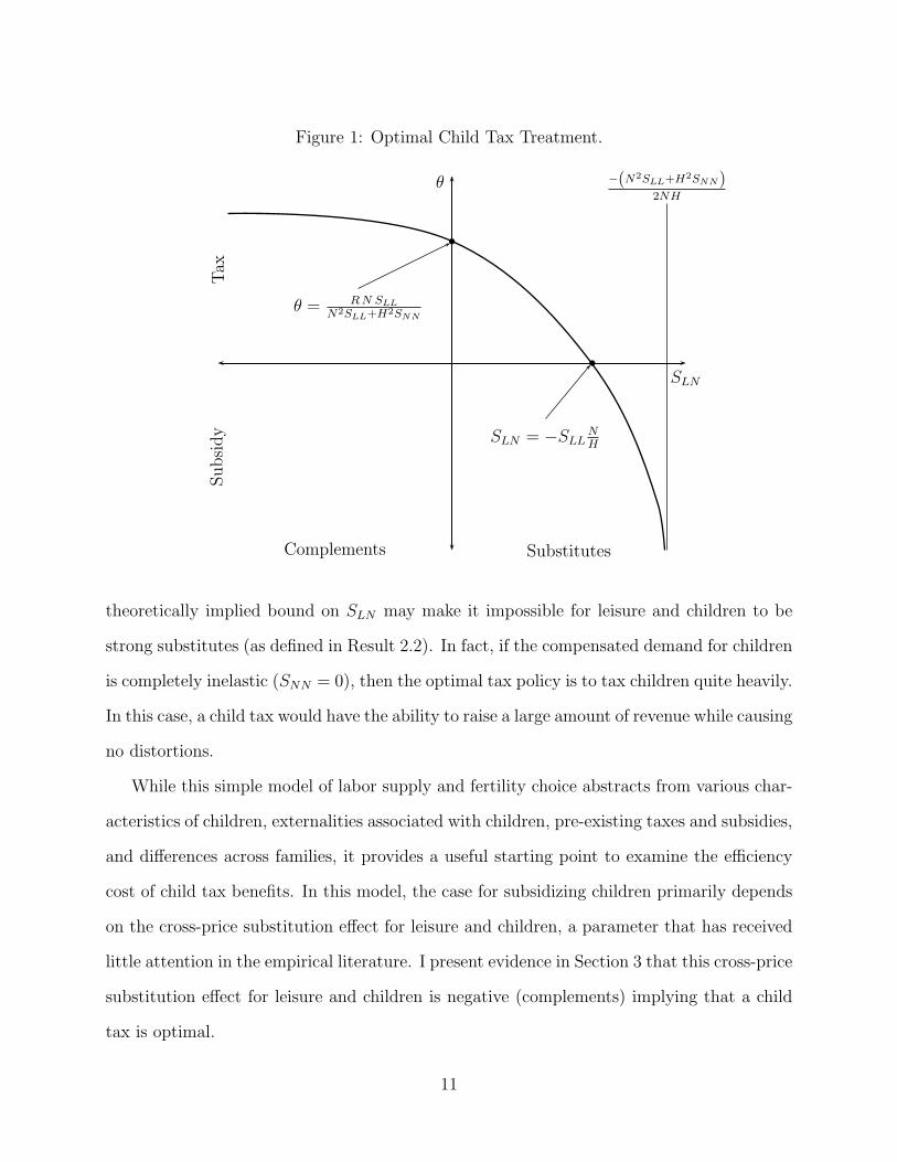
Figure 1: Optimal Child Tax Treatment.

θ

SLN

Complements Substitutes

Tax

Subsi

dy

−(N2SLL+H2SNN)2NH

θ = R N SLL

N2SLL+H2SNN

SLN = −SLLNH

theoretically implied bound on SLN may make it impossible for leisure and children to be

strong substitutes (as defined in Result 2.2). In fact, if the compensated demand for children

is completely inelastic (SNN = 0), then the optimal tax policy is to tax children quite heavily.

In this case, a child tax would have the ability to raise a large amount of revenue while causing

no distortions.

While this simple model of labor supply and fertility choice abstracts from various char-

acteristics of children, externalities associated with children, pre-existing taxes and subsidies,

and differences across families, it provides a useful starting point to examine the efficiency

cost of child tax benefits. In this model, the case for subsidizing children primarily depends

on the cross-price substitution effect for leisure and children, a parameter that has received

little attention in the empirical literature. I present evidence in Section 3 that this cross-price

substitution effect for leisure and children is negative (complements) implying that a child

tax is optimal.

11

2.2 Heterogeneous Agents with a Nonlinear Income Tax

The main result from the representative agent model, that it is optimal to tax children, is

confirmed in a model with heterogeneous agents that face a nonlinear income tax. As in the

representative agent model, utility depends only on leisure time, l, the number of children,

n, and consumption of other goods, c. However, there are many agents that differ in their

wage rates, w, but have identical utility functions. The distribution of agent wage rates is

given by the density function f(w). Hours of work is given by h, the time endowment minus

leisure time, l. The aggregate level of consumption, C is given by∫

∞

0c(w)f(w)dw, where

c(w) is the level of consumption chosen by an agent of wage type w. Similarly, the total

number of children, N , is given by∫

∞

0n(w)f(w)dw, where n(w) is the number of children

chosen by an agent of wage type w.

The government imposes a nonlinear income tax, t(wh), and a tax on children of θ. Note

that as before, a positive value for θ is a tax on children while a negative value for θ is a

child subsidy. The government’s objective is to maximize social welfare,

∫

∞

0

W (U(w)) f(w)d(w), (11)

where W is the social welfare function and U(w) is the utility of an agent of wage type w.

The government must raise revenue R which implies the following budget constraint:

∫

∞

0

t (wh(w)) f(w)d(w) +

∫

∞

0

θn(w)f(w)d(w) = R. (12)

Under standard assumptions on the utility and social welfare function, a progressive

nonlinear income tax may cause some agents to reduce their labor supply h to imitate the

wage types that are just below them. Following Mirrlees (1971), an agent’s utility must rise

with the wage type at a sufficient rate to prevent this mimicking behavior. This incentive

12

constraint is given by

dU (w)

dw=

∂U (c, l, n)

∂l

h

w=

Ulh

w. (13)

The government chooses the function t(wh) and θ to maximize (11) subject to (12) and

(13). Following Atkinson and Stiglitz (1976), the Hamiltonian is expressed as:

H(U,w, n, h, λ, µ) = W (U(w)) f(w) + λ (wh(w) − n(w) − R) f(w) − µ(w)Ulh

w. (14)

Maximizing this expression with respect to θ and substituting the agent’s first order condi-

tions yields the optimal tax formula:14

θ =µ(w)

λUc

h(w)

wf(w)(Uln − Ulc) (15)

The Atkinson-Stiglitz result, that no differential commodity taxation is optimal (i.e. no

subsidization or taxation of children in this model), depends on the assumption of labor

being weakly separable. Weak separability implies that Ulc and Uln are both zero. Thus, the

optimal tax treatment of children, θ, is zero if we assume weak separability.15 However, if

Uln and Ulc are not zero, then some special tax treatment of children is optimal.

If leisure and children are complements, this implies that as the agent increases the

amount of leisure time, the relative value of children to other consumption rises (∂Un/∂l >

∂Uc/∂l). The other terms in (15) including µ and λ are all positive. Thus, the optimal

value of θ is positive if leisure and children are complements. This result shows that the

intuition from the representative agent model - that it is optimal to tax families with children

- extends to a model with wage heterogeneity and a nonlinear income tax.

The assumption that the government does not allow θ to depend on the wage type w may

be important. While I suspect that allowing the government to select a function θ(w) would

14See Salanie (2003)or Kaplow (2008a) for an explanation of how to arrive at this optimal tax formula15Kaplow (2006) shows that under the assumption of weak separability, even if the nonlinear income tax

is not optimal, it is not optimal to have differential commodity taxation.

13

not change the overall result, I have not shown this. It is possible that the optimal θ(w)

would take on a negative value (a subsidy) for some wage types. Even with identical utility

functions, a good can be a leisure compliment for some wage types and a leisure substitute

for others.

Another important assumption is that there is no time cost of raising children. With time

costs, an agent’s choice of children is correlated with the wage, and therefor the government

can use the observability of the number of children to better infer an agent’s wage. Because a

higher wage rate would mean higher time costs, observing the number of children would be a

signal to the government about the agent’s wage type. Thus a child subsidy may be optimal.

As shown in the appendix, the inclusion of a time cost in the representative agent model does

not change the result that is it is optimal to tax children. However, the simple numerical

simulations in Section 4 suggest that adding time costs to this model with heterogeneous

agents can lead to the optimality of child subsidies. If the marginal utility of consumption

increases strongly in the number of children, this imply that transfers to agents with more

children are optimal.

3 Leisure and Children Cross-Price Effect Estimation

3.1 Data

The objective in this section is to estimate the cross-price substitution effect for leisure and

children. The data for this exercise is a sample of women from the 1979 National Longitudinal

Survey of Youth (NLSY). The NLSY contains detailed labor supply and fertility information

for each respondent from 1979 to 2004. The sample is restricted to women who were 16 to 20

when first interviewed in 1979. This restriction enables labor supply and earnings histories

to be constructed from age 19 until age 43. The number of children born to each woman by

14

age 43 is also obtained.16

The women in the sample were interviewed annually from 1979 to 1994 and then bi-

ennially from 1996 to 2004. Missed interviews do not necessarily prevent the construction

of a complete labor supply history because interviewers attempt to ask questions from the

previous interviews if missed. However, multiple missed interviews, especially if consecutive,

do prevent the creation of the labor supply history. Women for which it is not possible to

construct a complete labor supply or fertility history are dropped from the sample.

The decision to use a sample of women rather than a sample of married couples is

motivated by the fact that approximately one-third of all births in the United States are

to unmarried women. This is not simply due to teenage mothers. While about 90 percent

of teenage mothers are unmarried at the time they give birth, teenage mothers make up

less than a quarter of the total number of births to unmarried women each year. Births to

unmarried women age 20 or higher accounted for 26 percent of total births in 2003 (Martin

et al., 2005).

Three relationship categories are defined: married, partnership, single. Nearly all of

the women in the sample are single at age 19 and about 88 percent are married for some

period of time between age 19 and 43. Only 8 percent never report being married or in

a partnership. Some women move between relationship categories several times and the

relationship history is taken as exogenous. Like the relationship status, the labor supply and

earnings of husbands and partners is also taken as exogenous.17 Male and other income is

16For the youngest cohort, birth at age 42 is assumed if pregnancy is reported in 2004. Some women inthe sample may have children after age 43 and we would ideally have this in the data; however, this wouldbe only a small number of births. The U.S. National Center for Health Statistics reports that less than 1percent of women have a child after age 40 and that only 0.05 percent of women have a child after age 45(Martin et al., 2005).

17This requires the addition of nonwage income to the model of Section 2. The agent’s budget constraintbecomes:

T (1 − τ) + M(1 − τ) = C + L(1 − τ) + N(1 + θ)

where M is male earnings and other nonwage income (including transfer payments). The government budgetconstraint is also adjusted to reflect this addition:

R = τH + τM + θN.

15

subject to the linear income tax, but does not respond to changes in tax treatment. This

common assumption is often justified by the finding that the labor supply elasticity for

men is very low. For example, MaCurdy, Green, and Paarsch (1990) estimate that both

the substitution and income effects for male labor supply are close to zero.18 The choice

variables in this aplication of the representative agent model are the average labor supply of

the woman (age 19 to 43) and the total number of children that she has. The average hours

of market work over this period is created from a series of more than a thousand questions

asking how many hours she worked week by week over the previous period.19

After removing observations that do not have complete birth, work, and earnings histo-

ries, the sample used in this analysis consists of 4,169 of the 6,283 women in the NLSY. All

dollar amounts are inflation-adjusted to year 2000 dollars using the CPI-U before averaging.

An implied wage is calculated as the real average annual earnings divided by the average

annual hours. The summary statistics for this sample are given in Table 2.

The married, partner, and single variables measure the fraction of time from age 19

until 43 that the individual is either married, living with a partner, or single. The income

of the husband or partner as well as any nonwage income, including welfare benefits, are

combined into a single nonwage income variable. The “moved” variable indicates whether

the individual’s family moved to a different town while she was growing up. The summary

statistics for variables indicating whether the individual lived with both biological parents

until age 14 and whether either parent is an immigrant are also listed.

For those women with no reported hours of market work over the full time period, no

wage calculation can be made. This is unfortunate because an observed wage rate is essential

in estimating the cross-price substitution effect for leisure and children. Therefore, the

18There is considerable evidence that investment and other non-wage income is quite responsive to thetax treatment, thus a worthwhile extension of the model that I have not attempted would be to explicitlymodel investment behavior.

19This measure of the average hours of work does not distinguish between a part-time worker who isemployed continuously from age 19 to 43 and a full-time worker who is employed for only half that timeperiod.

16

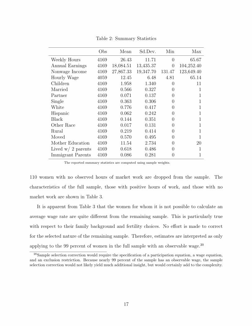
Table 2: Summary Statistics

Obs Mean Sd.Dev. Min Max

Weekly Hours 4169 26.43 11.71 0 65.67Annual Earnings 4169 18,084.51 13,435.37 0 104,252.40Nonwage Income 4169 27,867.33 19,347.70 131.47 123,649.40Hourly Wage 4059 12.45 6.48 4.81 65.14Children 4169 1.958 1.340 0 11Married 4169 0.566 0.327 0 1Partner 4169 0.071 0.137 0 1Single 4169 0.363 0.306 0 1White 4169 0.776 0.417 0 1Hispanic 4169 0.062 0.242 0 1Black 4169 0.144 0.351 0 1Other Race 4169 0.017 0.131 0 1Rural 4169 0.219 0.414 0 1Moved 4169 0.570 0.495 0 1Mother Education 4169 11.54 2.734 0 20Lived w/ 2 parents 4169 0.618 0.486 0 1Immigrant Parents 4169 0.086 0.281 0 1

The reported summary statistics are computed using sample weights.

110 women with no observed hours of market work are dropped from the sample. The

characteristics of the full sample, those with positive hours of work, and those with no

market work are shown in Table 3.

It is apparent from Table 3 that the women for whom it is not possible to calculate an

average wage rate are quite different from the remaining sample. This is particularly true

with respect to their family background and fertility choices. No effort is made to correct

for the selected nature of the remaining sample. Therefore, estimates are interpreted as only

applying to the 99 percent of women in the full sample with an observable wage.20

20Sample selection correction would require the specification of a participation equation, a wage equation,and an exclusion restriction. Because nearly 99 percent of the sample has an observable wage, the sampleselection correction would not likely yield much additional insight, but would certainly add to the complexity.

17

Table 3: Sample Average by Hours of Work

All Hours > 0 Hours = 0

Observations 4,169 4,059 110Sample Weight 1 0.985 0.015Weekly Hours 26.43 26.83 0Annual Earnings 18,084.51 18,362.11 0Nonwage Income 27,867.33 28,001.11 19,152.40Hourly Wage 12.45 12.45 -Children 1.958 1.944 2.856Married 0.566 0.569 0.366Partner 0.071 0.070 0.123Single 0.363 0.361 0.511White 0.776 0.782 0.394Hispanic 0.062 0.060 0.191Black 0.144 0.140 0.382Other Race 0.017 0.017 0.033Rural 0.219 0.220 0.132Moved 0.570 0.571 0.517Mother Education 11.54 11.57 9.20Both Parents (14) 0.616 0.618 0.439Immigrant Parents 0.086 0.086 0.111

The reported summary statistics are computed using sample weights.

3.2 Estimation

A common approach to estimating a substitution effect in a static model is to estimate a

linear demand equation that includes a wage variable and a nonwage income variable. This

is particularly common in the labor supply literature where an econometrician estimates a

labor supply function of this form:

Hoursi = α0 + α1 Wagei + α2 Nonwage Incomei + α3 Xi + ǫi. (16)

The vector Xi represents the predetermined characteristics of the individual that are observed

by the econometrician and ǫi represents those unobserved characteristics that affect labor

supply. A true labor supply function would depend not only on the wage, but also on the

18

prices of all other goods. In practice, other prices are not frequently included in the regression

equation, particularly when using cross-sectional data. The usual assumption used to justify

this is that the prices for all other goods are not individual-specific. Among other things,

this assumption implies that there are no geographical differences in other prices.

In the labor supply equation, α1 is the change in labor supply due to a one dollar increase

in the hourly wage. This total effect is comprised of an income effect and a substitution effect

as given by the Slutsky equation:

∂Hours

∂Wage=

(

∂Hours

∂Wage

)c

+ Hours∂Hours

∂Income. (17)

This same approach to estimating an own-price substitution effect for labor supply (or

leisure demand) can be used to estimate the cross-price substitution effect for leisure and

children. We specify a linear child demand function that depends on the wage, nonwage

income, a vector of predetermined and observed characteristics, and an error term that

represents those unobserved characteristics that affect child demand:

Childreni = β0 + β1 Wagei + β2 Nonwage Incomei + β3 Xi + ηi. (18)

Ideally, the “price” of children (cost of raising children) should also be included in this

specification. The absence of this variable is cause for some concern because the demand

of a good clearly depends on its own price. The high degree of uncertainty about the level

of expenditure required to raise a child–and how this level changes with family size, family

income, and other factors–severely complicates determining an individual-specific cost of

raising a child. Similar to the argument for the exclusion of other prices in a labor supply

equation, one could argue that there is little individual specific variation in the direct cost of

raising a child. However, differences in child tax benefits by income level, family economies

of scale, and geographical differences in the cost of food, housing, and health care suggest

19

that this may not be the case. The direction of any bias in the estimates of β1 and β2 from

this heterogeneity in the cost of raising children is not clear.

Thus, for this exercise, we make the assumption that there are no individual differences

in the monetary cost of children. This does not rule out differences in the opportunity cost

of raising children. Rather, the assumption is that each woman faces the same out-of-pocket

expenditure necessary to raise a child. If it were possible to determine an individual specific

PNi, this variable could be used in an alternative method for identifying the cross-price

substitution effect for leisure and children: a regression of labor supply on PNi, the wage

rate, and nonwage income.

For the identification of β1, there is a serious concern that the decision to have a child has

a direct influence on the wage. For example, Miller (2006) shows that the timing of the first

birth has a strong effect on a woman’s future wage growth. The child demand equation in

this paper is in regards to the number of children, not the timing of children, thus the Miller

(2006) result does not apply directly. A valid instrument for wage in the child demand

equation is a predetermined characteristic that affects the individual’s wage but not the

demand for children or other factors that affect the demand for children. Several observed

characteristics like the month and year of birth and measures of the reading habits of the

individual’s parents satisfy the definition in this sample. However, instrumental variables

estimation gives very similar estimates of β1 as OLS and using a Hausman test of endogeneity,

we fail to reject that the wage is exogenous.21 This is not conclusive evidence, however, the

assumption that the wage is exogenous is maintained in the discussion that follows.

Using the estimates for β1 and β2, the cross-price substitution effect for leisure and

21The two-stage least squares results are available from the author by request. In each regression, theestimate of β1 was larger in magnitude (more negative, although not statistically different) using instrumentalvariables estimation than the corresponding OLS regression. If having an additional child (not the timing ofthe birth) had a direct effect on the wage, one would expect the instrumental variables estimation to produceestimates of β1 that were smaller in magnitude.

20

children are given by (β1 − Hours β2) as indicated by the Slutsky decomposition:

∂Children

∂Wage=

(

∂Children

∂Wage

)c

+ Hours∂Children

∂Income. (19)

In the representative agent model of Section 2, we normalize the units of all goods so that

prices are unity. This same normalization is easily made to the total, income, and substitu-

tion effects by multiplying through by the appropriate prices:

SLN = PN

(

PLβ1 − Hβ2

)

. (20)

Given this normalization, SLN is the change in the compensated demand for children for a

doubling of the wage. At the average wage in the sample, a 100 percent wage increase would

place it at about the 95th wage percentile.

The estimation of equation (18) is given in Table 4. The region controls include indicators

for the region of the country the individual was raised in, either the Northeast, South,

Central, or West. The family controls provide information about the family during the

woman’s growing-up years, whether it was a rural or urban area, if the family had access to

a local library, and if the family ever moved. Also included is the number of siblings and

indicators for oldest or youngest child, immigrant parents, and if the woman grew up in a

home with both biological parents.22 Religion controls are for the religion that the individual

was raised in and also a measure of how often the family went to religious services.23

There are several issues to consider in this type of estimation. Concern is often expressed

about the measurement of nonwage income. The NLSY income variables are top-coded

22Youngest child is an indicator that the individual has at least one sibling and was the youngest child inher family; oldest child indicates that the individual has at least one sibling and was the oldest child in herfamily.

23Included in these variables are indicator for being raised in a family that went to religious servicestwice a month or more and an indicator of having converted to a religion other than the religion raised in.The religion categories (in order of size in the sample) are: Catholic, Baptist, Other Christian Religion,Methodist, Lutheran, Presbyterian, None, Pentecostal, Episcopalian, Jewish, and Non-Christian Religion.

21

Table 4: Linear Child Demand Estimation

(1) (2) (3) (4) (5)

Wage -0.0308 -0.0232 -0.0160 -0.0157 -0.0229(0.0031)** (0.0032)** (0.0031)** (0.0031)** (0.0032)**

Nonwage Income 0.0191 0.0206 0.0080 0.0078 0.0203(thousands) (0.0011)** (0.0011)** (0.0013)** (0.0013)** (0.0011)**Hispanic 0.603 0.316 0.383 0.374 0.309

(0.086)** (0.092)** (0.089)** (0.093)** (0.096)**Black 0.499 0.331 0.615 0.575 0.281

(0.061)** (0.062)** (0.062)** (0.065)** (0.065)**Other race -0.029 -0.229 -0.059 -0.020 -0.182

(0.154) (0.152) (0.147) (0.156) (0.161)Married 1.372 1.372

(0.080)** (0.080)**Partner 0.571 0.593

(0.153)** (0.153)**Constant 1.701 1.996 1.156 1.208 1.918

(0.072)** (0.133)** (0.084)** (0.165)** (0.162)**

Region controls yes yes yes yes yesFamily controls no yes yes yes yesReligion controls no no no yes yes

Observations 4059 4059 4059 4059 4059R-squared 0.1005 0.1422 0.2020 0.2063 0.1473

Total Effect -0.383 -0.289 -0.199 -0.195 -0.285Income Effect 0.351 0.378 0.147 0.143 0.373Substitution Effect -0.734 -0.667 -0.346 -0.339 -0.658

* significant at 5% ** significant at 1%. The reported values are computed using sample weights.Standard errors in parentheses.

Region controls include: northeast, central, and south. Family controls include: number of siblings,youngest child indicator, oldest child indicator, biological parents (14), immigrant parents, mother’seducation level, rural, moved, and a library indicator. Religion controls include: Catholic, Baptist,Methodist, Lutheran, Presbyterian, Pentecostal, Episcopalian, Jewish, Other Christian Religion, Non-Christian Religion, and a measure of frequency of attendance.

22

which puts a downward bias on both the average wage and the average nonwage income for

an individual. The cutoff at which top-coding occurs and the procedure have changed over

the 25 years of the survey. However, the number of individuals affected by top-coding is

small. A second concern is that the procedure for calculating nonwage income is to subtract

female earnings from total family income. This means that transfer payments that may

not be independent of female earnings are included in the measure of nonwage. However,

transfer payments are generally non-taxable and thus treating them as nonwage income is

more appropriate. A third issue is the problem of nonresponse to income questions. Nearly

all respondents in the NLSY report their own income and their spouse’s income, however,

approximately 30 percent of respondents living with a partner in a given year do not report

their partner’s income.24 Even if the individual keeps her finances completely separate from

her partner’s, living together suggests that they probably share some common expenses like

rent or house payments. Quite often, a woman who refuses to answer the partner’s income

question will answer the question in the next year and since the average woman in the sample

spends only about 7 percent of her time in a partnership, the nonresponse bias is likely small.

A regression of the percentage of the time living with a partner on other factors including

wage, race, region, and religion reveals very little correlation between time living with a

partner and any other characteristics.25

The assumption of a linear child demand function implies a specific form of the utility

function.26 An alternate functional form assumption for the direct utility could yield different

estimates for the substitution effects. Using OLS to estimate the child demand function may

24In the NLSY, partner income is not included in the constructed total family income variable. Forthis study, partner income was added to the constructed family income variable and then the respondent’searnings were subtracted to give nonwage income. Note that from 1979-1994 the partner income variablesare separate from spouse income variables, but after 1994, these variables are combined.

25This regression shows that women who live in the west and those who have lower wage rates spendmore time living with a partner. None of the religion variables were significantly different than zero. TheR-squared from the regression was 0.021, implying that the variables used in this analysis are not stronglycorrelated with time spent living with a partner.

26See Pencavel (1986) for a discussion of the direct and indirect utility functions implied by linear demandequations.

23

also be inappropriate because of the nature of the dependent variable. For example, it is

not possible for a woman to have a negative number of children. As Figure 2 shows, there

is more bunching at zero than would be expected if children were distributed normally.

While this suggests the possibility of censoring at zero (because individuals cannot have a

negative number of children), the more serious issue is that the dependent variable that is

not even approximately continuous and thus the normally distributed error term is probably

not reasonable. The dependent variable in this exercise takes on only 12 different values,

the natural numbers from 0 to 11. A discrete distribution, such as the Poisson is commonly

used for this type of count data.

Figure 2: Number of Children Histogram

0

0.1

0.2

0.3

0.4

ChildrenDensity computed using NLSY sample weights.

0 1 2 3 4 5 6 7 8 9 10 11

The Poisson distribution is determined by a single parameter, µ that indicates the in-

tensity of the Poisson process. The value of µ is both the mean and the variance of the

distribution. Thus, we only need to specify µ = E(childreni|wagei, nonwage incomei, Xi),

which we assume is given by the exponential function:

E (childreni|wagei, nonwage incomei, Xi) = e(β0+β1wageiwage+β2nonwage incomei+β3Xi). (21)

This specification assures that µ will be positive for all values of wage, nonwage income, and

X. In this model, the probability that the number of children equals the value j, conditional

24

on the independent variables, is

Pr(children = j|X) =e(−e(Xβ)) (

e(Xβ))j

j!for j = 0, 1, 2, . . . (22)

where X represents the full set of explanatory variables, including wage and nonwage income.

Maximum likelihood estimation is used to obtain the parameter estimates. The estimated

marginal effects evaluated at the mean are reported as the first two columns of Table 5.

Table 5: Poisson and Ordered Probit Child Demand Estimation

Poisson Poisson Ordered Probit Ordered Probit

Wage -0.0170 -0.0252 -0.0148 -0.0208(0.0051)** (0.0056)** (0.0040)** (0.0042)**

Nonwage Income 0.0074 0.0185 0.0074 0.0183(thousands) (0.0013)** (0.0011)** (0.0013)** (0.0012)**Hispanic 0.347 0.281 0.319 0.244

(0.081)** (0.082)** (0.068)** (0.066)**Black 0.646 0.282 0.545 0.235

(0.075)** (0.066)** (0.059)** (0.054)**Other race 0.006 -0.168 -0.005 -0.162

(0.216) (0.194) (0.197) (0.183)Married 1.450 1.356

(0.093)** (0.086)**Partner 0.792 0.635

(0.204)** (0.171)**

Region controls yes yes yes yesFamily controls yes yes yes yesReligion controls yes yes yes yes

Observations 4059 4059 4059 4059

Total Effect -0.212 -0.314 -0.184 -0.259Income Effect 0.136 0.340 0.136 0.336Substitution Effect -0.348 -0.653 -0.320 -0.595

* significant at 5% ** significant at 1%. The reported values are computed using sample weights.Standard errors in parentheses.

Region controls include: northeast, central, and south. Family controls include: number of siblings,youngest child indicator, oldest child indicator, biological parents (14), immigrant parents, mother’seducation level, rural, moved, and a library indicator. Religion controls include: Catholic, Baptist,Methodist, Lutheran, Presbyterian, Pentecostal, Episcopalian, Jewish, Other Christian Religion, Non-Christian Religion, and a measure of frequency of attendance.

25

As an alternative, an ordered probit model is also considered. The model is built around

the concept of a latent demand for children that, conditioning on X, is normally distributed.

This latent demand for children is continuously distributed with nothing preventing it from

taking on negative values. However, this latent demand is not observed. What we do observe

is the actual number of children (0, 1, 2, . . .) selected by each individual. A set of cutoff values

for the latent variable, for example {0.5, 1.5, 2.5, 3.5, . . .}, determine the observed number of

children. If the latent variable were to have a value that falls between 0.5 and 1.5 (given

the cutoff values in the example) then the individual would choose to have one child. The

cutoff values and parameter estimates are obtained by maximum likelihood estimation. The

estimated marginal effects evaluated at the mean are reported as the third and fourth columns

of Table 5.

The results reported in Table 5 are consistent with those of Table 4 (page 22). A one

dollar increase in the life time average hourly wage (evaluated at the mean wage) is associated

with a decrease in the number of children between 0.014 and 0.031. The estimated income

effect is positive, meaning that children are a normal good. Thus, the negative total effect

implies that the substitution effect is larger in magnitude than the income effect.

For some, a positive value for the estimated income effect is perhaps surprising. It is

sometimes claimed that high-income countries have lower fertility rates due to a negative

income effect.27 These results are contrary to that claim. In fact, it is apparent from an

examination of the unconditional average number of children by average annual real family

income level that the number of children increases with income (see Figure 3). These results

support the claim that higher female wages are an important factor in explaining fertility

decline (Butz and Ward 1979; Schultz 1985; Heckman and Walker 1990).28

27See Jones, Schoonbroodt, and Tertilt (2008) for a discussion of the relationship between income andfertility.

28While it is argued that rising female wages in the last half of the 20th Century is an important explanationfor the decline in fertility rates, it should be noted that fertility rates in the United States began to declinein the late 19th Century, long before any sizable increase in female wages.

26

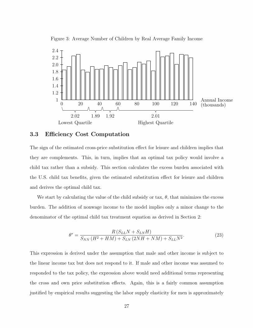
Figure 3: Average Number of Children by Real Average Family Income

0 20 40 60 80 100 120 1401

1.2

1.4

1.6

1.8

2.0

2.2

2.4

Annual Income(thousands)

2.02

Lowest Quartile

1.89 1.92 2.01

Highest Quartile

3.3 Efficiency Cost Computation

The sign of the estimated cross-price substitution effect for leisure and children implies that

they are complements. This, in turn, implies that an optimal tax policy would involve a

child tax rather than a subsidy. This section calculates the excess burden associated with

the U.S. child tax benefits, given the estimated substitution effect for leisure and children

and derives the optimal child tax.

We start by calculating the value of the child subsidy or tax, θ, that minimizes the excess

burden. The addition of nonwage income to the model implies only a minor change to the

denominator of the optimal child tax treatment equation as derived in Section 2:

θ∗ =R (SLLN + SLNH)

SNN (H2 + HM) + SLN (2NH + NM) + SLLN2. (23)

This expression is derived under the assumption that male and other income is subject to

the linear income tax but does not respond to it. If male and other income was assumed to

responded to the tax policy, the expression above would need additional terms representing

the cross and own price substitution effects. Again, this is a fairly common assumption

justified by empirical results suggesting the labor supply elasticity for men is approximately

27

zero (MaCurdy, Green, and Paarsch, 1990).

We need estimates of each of the parameters in order to evaluate the expression. Sample

averages for annual female earnings ($18,362), nonwage and male income ($28,001), and

children (1.944) as reported in Table 3 (page 18) provide values for H and M . We also need

an estimate of the cost of raising a child, PN . There are various estimates of PN in the

literature and rather than make a judgment on which estimate is best, we will proceed by

selecting two values: one high and the other low. For the high value, the USDA calculates

that the average annual child-related expenditure for a middle-income married couple is

about $11,000 (Lino, 2007). The USDA method measure education and clothing expenditure

on children and also attributes a portion of food, housing, utilities, and transportation to

children. For the low value, the U.S. poverty thresholds increase with the number in the

household and this implies a cost of raising a child of about $3,400. The high value implies

N = 21, 384; the low value implies N = 6, 610. The Congressional Budget Office reports

that taxpayers paid an average of $6,100 in federal income tax in 2003, so I take this as the

value for R.29

Estimation of the own-price substitution effect for children, SNN , is not possible with this

data because there is no observed cross-sectional variation in the cost of raising children.

Gauthier and Hatzius (1997) find evidence of a smallfertility response in a panel of 22

countries. Huang (2002) also found a small fertility response using times series data from

Taiwan. Baughman and Dickert-Conlin (2003) find no fertility response to EITC increases for

unmarried women and only a small positive response for married women. For the calculation,

I use an estimate from Laroque and Salanie (2005) which uses a structural model of labor

supply and fertility to explain the fertility response of families in France. They estimate the

uncompensated cost elasticity of the demand for children to be about 0.2. This value implies

that doubling the cost of children would reduce the total number of children born over a

29See the CBO document “Historical Effective Federal Tax Rates: 1979 to 2003” located on the web at:http://www.cbo.gov/ftpdocs/70xx/doc7000/12-29-FedTaxRates.pdf. The CBO reports that taxpayers in2003 paid an average of $14,200 in federal taxes, 43 percent of which was due to the individual income tax.

28

woman’s life time by 0.39 children on average. This uncompensated effect is the sum of the

substitution effect, SNN , and the income effect. The own-price substitution effect implied

by the Laroque and Salanie (2005) estimate is -0.377.

An estimate for the own-price substitution effect for leisure, SLL can be obtained by the

same method as was used to estimate of the cross-price substitution effect for leisure and

children. Using the same NLSY sample of women, I estimate the effect of wages and non-

wage income on labor supply, assuming that labor supply is given by a linear function as in

equation (16). The results indicate that a dollar increase in a woman’s average hourly wage

leads to an increase of approximately 0.48 hours per week of market work. The female labor

supply elasticities implied by this result seem reasonable, the compensated wage elasticity

is 0.344 and the uncompensated wage elasticity is 0.224, well within the range of estimated

elasticities in the female labor supply literature(Killingsworth and Heckman, 1986).

Using the high or the low estimate for the cost of raising a child makes a large difference

in the size of the optimal child tax. Using the low value for PN of $3,400 results in an

optimal child tax of about $100 per child. Using the high value for PN of $11,000 results

in an optimal child tax of about $800 per child. The reason for the large difference is that

if children are quite expensive, then a child tax has the ability to raise a large amount of

revenue and thus allow for lower income tax rates while at the same time causing very little

distortion in the demand for children. If children are much less expensive, then a large tax

would be much more distortive.

The optimal linear income tax rate derived from this method is quite low, 12.7 percent

under low child costs and 9.4 percent under high child costs. The linear income tax in this

model has no standard deduction or exemption so this is both the marginal and the average

tax rate. For comparison, in order to provide child tax benefits of $2,000 per child and still

raise the $6,100 revenue, a tax rate of 21.5 percent would be required.

The excess burden of the tax policy is a measure of the loss of welfare greater than would

29

have occurred if the tax revenue had been collected as a lump sum tax:

EB = −1

2

(

τ 2SLL + θ2SNN − 2τθSLN

)

. (24)

Under a lump sum tax this excess burden measure would have a value of zero. Under the

high child cost assumption, the optimal tax policy of a $800 per child tax and a 9.4 percent

flat income tax rate produces an excess burden of $25. If the government is not able to

impose a child tax and instead sets θ to zero, then the flat income tax rate would be 13.2

percent and the excess burden would be $52. In order for the government to provide a $2,000

per child subsidy, the excess burden would be $350. Under the low child cost assumption,

the excess burden of providing a $2,000 per child subsidy is $496. Thus, when considering

economic efficiency, the true cost of providing child tax benefits in the U.S. federal income

tax is in the $190 to $200 billion range.

4 Numerical Simulation with Time Costs

Consider a model in which there is a necessary time and monetary cost associated with

children. For example, if agents have Stone-Geary utility where at least one of the basic

needs parameters increases in the number of children, then providing child tax benefits

could increase social welfare. This is represented by the following utility function:

U(C,L,N) = β ln (C − f(N)) + (1 − β) ln (L − g(N)) + V (N) (25)

where f(N) is some necessary cost of raising a child which the agent does not consider

consumption and g(N) is some necessary time cost of raising a child which the agent does not

consider leisure. The function V (N) captures the direct utility from children. Expenditure on

children, either in time or money, above the necessary levels of f(N) and g(N) is respectively

30

considered consumption or leisure.

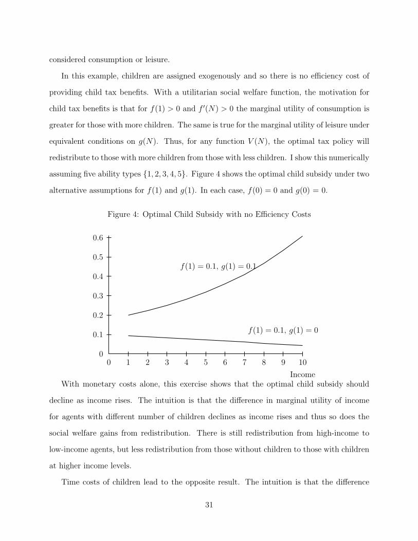
In this example, children are assigned exogenously and so there is no efficiency cost of

providing child tax benefits. With a utilitarian social welfare function, the motivation for

child tax benefits is that for f(1) > 0 and f ′(N) > 0 the marginal utility of consumption is

greater for those with more children. The same is true for the marginal utility of leisure under

equivalent conditions on g(N). Thus, for any function V (N), the optimal tax policy will

redistribute to those with more children from those with less children. I show this numerically

assuming five ability types {1, 2, 3, 4, 5}. Figure 4 shows the optimal child subsidy under two

alternative assumptions for f(1) and g(1). In each case, f(0) = 0 and g(0) = 0.

Figure 4: Optimal Child Subsidy with no Efficiency Costs

0 1 2 3 4 5 6 7 8 9 100

0.1

0.2

0.3

0.4

0.5

0.6

Income

f(1) = 0.1, g(1) = 0

f(1) = 0.1, g(1) = 0.1

With monetary costs alone, this exercise shows that the optimal child subsidy should

decline as income rises. The intuition is that the difference in marginal utility of income

for agents with different number of children declines as income rises and thus so does the

social welfare gains from redistribution. There is still redistribution from high-income to

low-income agents, but less redistribution from those without children to those with children

at higher income levels.

Time costs of children lead to the opposite result. The intuition is that the difference

31

in the marginal utility of income for those with different numbers of children increases in

the agents’ ability level and thus income level. An agent with a high ability level or wage

has a higher opportunity cost of the time spent raising children than an agent with a lower

ability level. Because the difference in the marginal utility of income increases in income,

the optimal child subsidy increases in income in models with only time costs.

In models with both monetary and time costs of raising children, the shape of the curve

depends on the relative importance of the two costs. In Figure 4, the top curve is increasing

in income because the time costs dominate the monetary costs. In this example, the time

required to raise a child is fixed, representing the amount of supervision, care, and adult

interaction that children need. However, in reality, there is no requirement that parents

spend all of that time. For high-ability agents, some time costs can be avoided by paying

for child care services. Thus, the monetary costs of raising a child may be more important

than the time costs.

5 Conclusion

The budgetary cost of child tax benefits in the U.S. is estimated to be $160 billion in 2008

and it will likely continue to grow. However, there has been little work analyzing these

child subsidies. In this paper, I use a representative agent model to show that the efficiency

costs depend on the cross-price substitution effect for children and leisure (non-market work)

time. If children and leisure are complements then child subsidies are not optimal in terms

of economic efficiency. Estimation of a child demand function using NLSY data indicated

that children and leisure are complements over the life cycle. A back of the envelope style

calculation of the optimal child tax implied by the estimates is in the range of $100 to $800

per child. However, this does not mean that it is optimal to tax children. These estimate

imply that there is a large efficiency cost in subsidizing children, but it is possible that the

benefits from these subsidies outweigh the costs.

32

There is a strong need for additional research on the optimal design of child subsidies.

The child tax benefits in the United States are large and expensive and have the potential to

grow even larger over the next few years. This is a research topic with far too little formal

analysis on which to base policy recommendations. Careful thinking about the efficiency

costs associated with child subsidies is only a first step. Further analysis of the consequences

of child subsidies, especially for different ranges in the income distribution, presents an

important area for future research.

References

Atkinson, A. B., and J. E. Stiglitz (1976): “The design of tax structure: direct versus indirect

taxation.,” Journal of Public Economics, 6, 55–75.

Auerbach, A. J. (1985): “The Theory of Excess Burden and Optimal Taxation,” in Handbook of

Public Economics, ed. by A. J. Auerbach, and M. Feldstein, vol. 1, pp. 61–127. Elsevier Science

Publishers B.V. (North-Holland).

Auerbach, A. J., and H. S. Rosen (1980): “Will the Real Excess Burden Please Stand Up?

(Or, Seven Measures in Search of a Concept),” NBER Working Paper: 0495, National Bureau

of Economic Research.

Baughman, R., and S. Dickert-Conlin (2003): “Did Expanding the EITC Promote Mother-

hood?,” American Economic Review, 93(2), 247–251.

Boskin, M. J., and E. Sheshinski (1983): “Optimal Tax Treatment of the Family: Married

Couples,” Journal of Public Economics, 20(3), 281–297.

Butz, W. P., and M. P. Ward (1979): “The Emergence of Countercyclical U.S. Fertility,” The

American Economic Review, 69(3), 318–328.

Corlett, W. J., and D. C. Hague (1954): “Complementarity and the Excess Burden of Taxa-

tion,” The Review of Economic Studies, 21(1), 21–30.

33

Diamond, P. A., and D. L. McFadden (1974): “Some Uses of the Expenditure Function in

Public Finance,” Journal of Public Economics, 3(1), 3–21.

Gauthier, A. H., and J. Hatzius (1997): “Family Benefits and Fertility: An Economic Analy-

sis.,” Population Studies, 51(3), 295–306.

Green, J. R., and E. Sheshinski (1979): “Approximating the Efficiency Gain of Tax Reforms,”

Journal of Public Economics, 11(2), 179–195.

Harberger, A. C. (1964): “The Measurment of Waste,” The American Economic Review, 54(3),

58–76.

Heckman, J. J., and J. R. Walker (1990): “The Relationship Between Wages and Income and

the Timing and Spacing of Births: Evidence from Swedish Longitudinal Data,” Econometrica,

58(6), 1411–1441.

Hicks, J. R. (1939): Value and Capital. Oxford: Oxford University Press.

Hotelling, H. (1938): “The General Welfare in Relation to Problems of Taxation and of Railway

and Utility Rates,” Econometrica, 6(3), 242–269.

Huang, J.-T. (2002): “Personal Tax Exemption: The Effect on Fertility in Taiwan,” The Devel-

oping Economies, XL(1), 32–48.

Jones, L. E., A. Schoonbroodt, and M. Tertilt (2008): “Fertility and Income in the Cross

Section: Theories and Evidence,” Mimeo.

Kaplow, L. (2006): “On the undesirability of commodity taxation even when income taxation is

not optimal,” Journal of Public Economics, 90, 1235–1250.

(2008a): “Taxing Leisure Complements,” NBER Working Paper, 14397.

(2008b): The Theory of Taxation and Public Economics. Princeton University Press.

34

Killingsworth, M. R., and J. J. Heckman (1986): “Female Labor Supply: A Survey,” in

Handbook of Labor Economics Volume 1, ed. by O. Ashenfelter, and R. Layard, pp. 103–204.

Amsterdam: North-Holland.

Laroque, G., and B. Salanie (2005): Does Fertility Respond to Financial Incentives? CEPR

Discussion Paper no. 5007. (http://www.cepr.org/pubs/dps/DP5007.asp).

Lino, M. (2007): “Expenditures on Children by Families, 2006,” U.S. Department of Agriculture,

Center for Nutrition Policy and Promotion, Miscellaneous Publication No. 1528-2006.

MaCurdy, T., D. Green, and H. Paarsch (1990): “Assessing Empirical Approaches for Ana-

lyzing Taxes and Labor Supply,” Journal of Human Resources, 25(3), 415–490.

Martin, J. A., B. E. Hamilton, P. D. Sutton, S. J. Ventura, F. Menacker, and M. L.

Munson (2005): “Births: Final Data for 2003,” National Vital Statistics Reports, 54(2).

Miller, A. R. (2006): “The Effects of Motherhood Timing on Career Path,” Mimeo, University

of Virginia.

Mirrlees, J. A. (1971): “An exploration in the theory of optimum income taxation,” Review of

Economic Studies, 38, 175–208.

Pencavel, J. (1986): “Labor Supply of Men: A Survey,” in Handbook of Labor Economics Volume

1, ed. by O. Ashenfelter, and R. Layard, pp. 3–102. Amsterdam: North-Holland.

Rosen, H. S. (1978): “The Measurement of Excess Burden with Explicit Utility Functions,”

Journal of Political Economcy, 86(2), S121–S135.

Salanie, B. (2003): The Economics of Taxation. The MIT Press, Cambridge, Massachusetts.

Schultz, T. P. (1985): “Changing World Prices, Women’s Wages, and the Fertility Transition:

Sweden, 1860-1910,” The Journal of Political Economy, 93(6), 1126–1154.

35

Appendix

Time Cost of Raising Children

Adding a time cost of raising children to the representative agent model does not change the result

that it is optimal to tax children. The model is altered so that the agent now faces a time constraint

that depends explicitly on children:

T = H + L + g(N). (A-1)

The function g(N) represents the time cost of raising children. The time cost likely increases in

the number of children, g′(N) > 0, but due to economies of scale in families, g′′(N) < 0. For

convenience, we scale the units of each good so that the wage and the monetary costs of children

are unity. The agent maximizes equation (1), subject to the following full income budget constraint:

T (1 − τ) = L(1 − τ) + g(N)(1 − τ) + C + N(1 + θ) (A-2)

where M is non-labor income.

By totally differentiating the first order conditions from the optimal tax problem, we derive

how the agent’s leisure and child choices are affected by τ and θ.

∂L

∂τ= −SLL − g′(N)SLN − HiL (A-3)

∂N

∂τ= −SLN − g′(N)SNN − HiN (A-4)

∂L

∂θ= SLN − NiL (A-5)

∂N

∂θ= SNN − NiN (A-6)

36

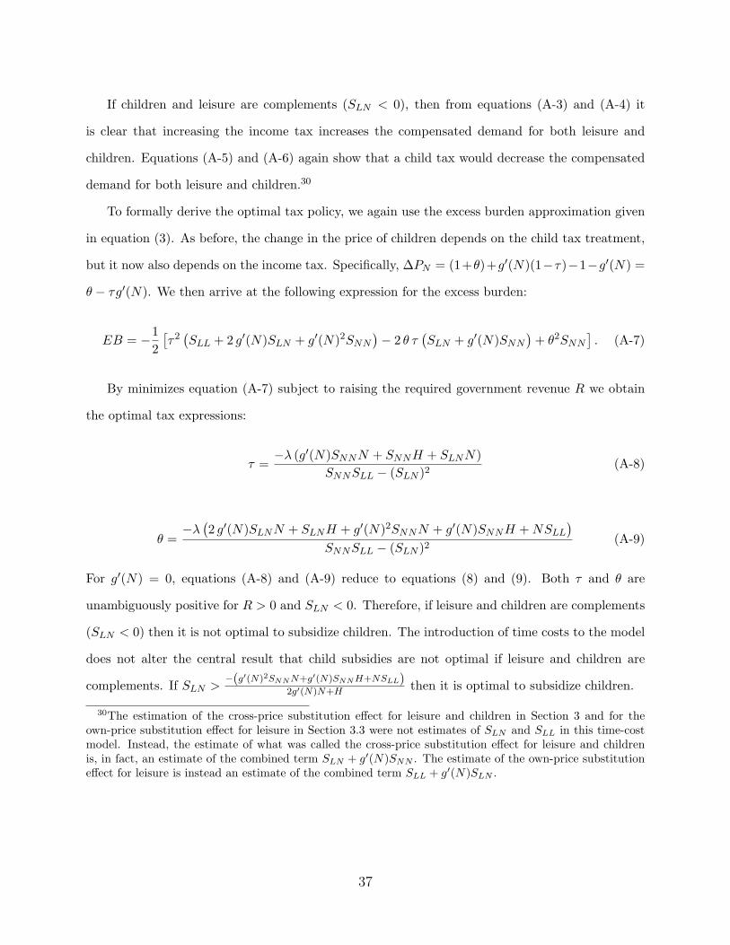
If children and leisure are complements (SLN < 0), then from equations (A-3) and (A-4) it

is clear that increasing the income tax increases the compensated demand for both leisure and

children. Equations (A-5) and (A-6) again show that a child tax would decrease the compensated

demand for both leisure and children.30

To formally derive the optimal tax policy, we again use the excess burden approximation given

in equation (3). As before, the change in the price of children depends on the child tax treatment,

but it now also depends on the income tax. Specifically, ∆PN = (1+θ)+g′(N)(1−τ)−1−g′(N) =

θ − τg′(N). We then arrive at the following expression for the excess burden:

EB = −1

2

[

τ2(

SLL + 2 g′(N)SLN + g′(N)2SNN

)

− 2 θ τ(

SLN + g′(N)SNN

)

+ θ2SNN

]

. (A-7)

By minimizes equation (A-7) subject to raising the required government revenue R we obtain

the optimal tax expressions:

τ =−λ (g′(N)SNNN + SNNH + SLNN)

SNNSLL − (SLN )2(A-8)

θ =−λ

(

2 g′(N)SLNN + SLNH + g′(N)2SNNN + g′(N)SNNH + NSLL

)

SNNSLL − (SLN )2(A-9)

For g′(N) = 0, equations (A-8) and (A-9) reduce to equations (8) and (9). Both τ and θ are

unambiguously positive for R > 0 and SLN < 0. Therefore, if leisure and children are complements

(SLN < 0) then it is not optimal to subsidize children. The introduction of time costs to the model

does not alter the central result that child subsidies are not optimal if leisure and children are

complements. If SLN >−(g′(N)2SNNN+g′(N)SNNH+NSLL)

2g′(N)N+Hthen it is optimal to subsidize children.

30The estimation of the cross-price substitution effect for leisure and children in Section 3 and for theown-price substitution effect for leisure in Section 3.3 were not estimates of SLN and SLL in this time-costmodel. Instead, the estimate of what was called the cross-price substitution effect for leisure and childrenis, in fact, an estimate of the combined term SLN + g′(N)SNN . The estimate of the own-price substitutioneffect for leisure is instead an estimate of the combined term SLL + g′(N)SLN .

37

After scaling N and L, the agent’s Lagrangean is:

L = U(C, L, N) + λ

[

T (1 − τ) + M − L (1 − τ) − g(N) (1 − τ) − C − N (1 + θ)

]

(A-10)

The first order conditions are:

∂L

∂C= UC − λ = 0 (A-11)

∂L

∂L= UL − λ(1 − τ) = 0 (A-12)

∂L

∂N= UN − λ

(

1 + g′(N) (1 − τ) + θ)

= 0 (A-13)

∂L

∂λ= T (1 − τ) + M − L (1 − τ) − g(N) (1 − τ) − C − N (1 + θ) = 0 (A-14)

Totally differentiating (A-11) - (A-14) and placing in matrix form, the system of differential equa-

tions is:

UCC UCL UCN −1

ULC ULL ULN (τ − 1)

UNC UNL UNN − λg′′(N)(1 − τ) g′(N)(τ − 1) − (1 + θ)

−1 (τ − 1) g′(N)(τ − 1) − (1 + θ) 0

dC

dL

dN

dλ

=

0

−λdτ

−λg′(N)dτ + λdθ

(T − L − g(N)) dτ + Ndθ + (1 − τ)dT + dM

(A-15)

The matrix above is called the bordered Hessian and is symmetric by Young’s Theorem. The

38

solution to the system is found by taking the inverse of the bordered Hessian matrix

(

Bordered Hessian

)

−1

=1

D

D11 D21 D31 D41

D12 D22 D32 D42

D13 D23 D33 D43

D14 D24 D34 D44

(A-16)

where D is the determinant of the bordered Hessian and Dij is the cofactor found by taking the

determinant of the bordered Hessian after deleting row i and column j. Note that the inverse of

the bordered Hessian is also symmetric. The solution to the system of equations is given by the

following expressions:

dC = −[

λD21

D+ λ g′(N)D31

D− H D41

D

]

dτ +[

λD31

D+ N D41

D

]

dθ +[

(1 − τ)D41

D

]

dT +[

D41

D

]

dM (A-17)

dL = −[

λD22

D+ λ g′(N)D32

D− H D42

D

]

dτ +[

λD32

D+ N D42

D

]

dθ +[

(1 − τ)D42

D

]

dT +[

D42

D

]

dM (A-18)

dN = −[

λD23

D+ λ g′(N)D33

D− H D43

D

]

dτ +[

λD33

D+ N D43

D

]

dθ +[

(1 − τ)D43

D

]

dT +[

D43

D

]

dM (A-19)

equations (A-3) - (A-6) in the text are derived by combining equations (A-18) and (A-19) with the

definitions of the Slutsky matrix:

SLC = λD21D

SNC = λD31D

iC = −D41D

SLL = λD22D

SNL = λD32D

iL = −D42D

SLN = λD23D

SNN = λD33D

iN = −D43D

.

Note that the symmetry of the inverse of the bordered Hessian matrix means that the Slutsky

matrix is also symmetric. This implies that the effect of a small increase in the price of good i on

the compensated demand of good j is identical to the effect of an equivalent increase in the price

of good j on the compensated demand of good i (Sij = Sji).

The excess burden approximation is given by:

EB = −1

2

[

∆PL

(

∂Lc

∂ττ +

∂Lc

∂θθ

)

+ ∆PN

(

∂N c

∂θθ +

∂N c

∂ττ

)]

(A-20)

39

Substituting in the compensated demand effects from equations (A-3) - (A-6) we obtain:

EB = −1

2

[

−τ(

(−SLL − g′(N)SLN ) τ + SLN θ)

+ (θ − τg′(N))(

SNN θ + (−SLN − g′(N)SNN ) τ)]

.

By simply rearranging terms, we arrive at equation (A-7) in the text. The Lagrangean for the

optimal tax problem is:

L = EB − λ (τH + θN − R) (A-21)

The first order conditions are:

∂L

∂τ= −λH +

1

2

(

SLNθ + τg′(N)(

−SLN − g′(N)SNN

)

+ g′(N)SNNθ)

−1

2

(

θ − τg′(N)) (

−SLN − g′(N)SNN

)

− τ(

SLL + g′(N)SLN

)

∂L

∂θ= −

1

2

(

SNNθ − τSLN + τ(

−SLN − g′(N)SNN

)

− SNN

(

θ − τg′(N)))

− λN

∂L

∂λ= τH + θN − R

Solving these first order conditions for τ and θ give the optimal tax policy expressions:

τ =R (g′(N)SNNN + SNNH + SLNN)

N2SLL + 2N2g′(N)SLN + N2g′(N)2SNN + 2NSLNH + 2Ng′(N)SNNH + SNNH2(A-22)

θ =R

(

2 g′(N)SLNN + SLNH + g′(N)2SNNN + g′(N)SNNH + NSLL

)

N2SLL + 2N2g′(N)SLN + N2g′(N)2SNN + 2NSLNH + 2Ng′(N)SNNH + SNNH2(A-23)

40