Efficiency-Adjusted Public Capital and Growth,. IMF ... · Efficiency-Adjusted Public Capital and Growth ... This paper constructs an efficiency-adjusted public capital stock series

WP/11/217

Efficiency-Adjusted Public Capital and Growth

Sanjeev Gupta, Alvar Kangur, Chris Papageorgiou, and Abdoul Wane

© 2011 International Monetary Fund WP/11/217

IMF Working Paper

Fiscal Affairs Department and Strategy, Policy, and Review Department

Efficiency-Adjusted Public Capital and Growth

Prepared by Sanjeev Gupta, Alvar Kangur, Chris Papageorgiou and Abdoul Wane1

September 2011

Abstract

This paper constructs an efficiency-adjusted public capital stock series and re-examines the public capital and growth relationship for 52 developing countries. The results show that public capital is a significant contributor to economic growth. Although the estimated coefficient for the income share of public capital is larger in middle- than in low-income countries, the opposite is true for the marginal product of public capital. The quality of public investment, as measured by variables capturing the adequacy of project selection and implementation, are statistically significant in explaining variations in economic growth, a result mainly driven by low-income countries.

JEL Classification Numbers: O19, O23, O40, O47

Keywords: Public capital stock, public investment efficiency, appraisal, selection, implementation and evaluation of public investment, growth accounting. Author’s E-mail Address: [email protected], [email protected], [email protected], [email protected]

1 We wish to thank Santiago Acosta, Chris Adam, Pierre-Richard Agénor, Andy Berg, Sambit Bhattacharyya, Hugh Bredenkamp, Francesco Caselli, Paul Collier, Benedict Clements, Era Dabla-Norris, Antonio David, Hamid Davoodi, Raphael Espinoza, Luc Eyraud, Cheikh Anta Gueye, Mick Keen, Aart Kraay, Nicola Limodio, Nkunde Mwase, Atsushi Oshima, Cathy Pattillo, Tigran Poghosyan, Rafael Romeu, Luis Serven, Kenichi Ueda, Rick van der Ploeg, Genevieve Verdier, and seminar participants at the University of Oxford and the IMF for helpful comments and suggestions on earlier versions of the paper.

This Working Paper should not be reported as representing the views of the IMF. The views expressed in this Working Paper are those of the author(s) and do not necessarily represent those of the IMF or IMF policy. Working Papers describe research in progress by the author(s) and are published to elicit comments and to further debate.

3

Contents Page

I. Introduction ............................................................................................................................4

II. Literature Review ..................................................................................................................5

III. A First Look at the Data.......................................................................................................7

IV. Public capital and Growth: Panel Regression Analysis .....................................................15 A. Estimation Method ..................................................................................................15 B. Results .....................................................................................................................17 C. Baseline Results ......................................................................................................17

V. Concluding Remarks ...........................................................................................................25 Tables 1. GDP Growth, Public Investment and Public Capital Stock Growth, 1960–2009 .................8 2. Public Investment Management Index (PIMI) by Income Group .......................................11 3. Unadjusted and PIMI-adjusted Public Capital Stock by Income Group .............................13 4. Growth Rate of Public Capital Stock by Income Group ......................................................13 5. Static Fixed Effects Regressions with PIMI-adjusted Public Capital ..................................17 6. Dynamic System GMM Regressions with PIMI-adjusted Public Capital ...........................18 7. Regressions for Public Investment Stage .............................................................................21 8. Results of Robustness Tests .................................................................................................23 Figures 1. Investment Ratio and Growth Rate of Public Capital ............................................................9 2. PIMI Distribution and Decomposition by Sub-Index ..........................................................11 3. Spearman Correlation Between PIMI and other Indicies ....................................................12 4. Unadjusted and PIMI-adjusted Capital Stock by Income Group.........................................14 5. Time-varying PIMI ..............................................................................................................22 Appendixes A. List of countries with Corresponding PIMI ........................................................................29 B. Details on the Construction of PIMI-adjusted Public Capital Stock Series ........................32 C. Initial Conditions and PIMI Effect on Efficiency Adjusted Capital ...................................33 D: Alternative Approach to Assessing the Effect of Different Stages of Public Investment on Aggregate Output ................................................................................................................34 E. Recovering the Parameters of the CES Production Function ..............................................36 References ................................................................................................................................26

4

I. INTRODUCTION

Many developing countries have a long legacy of failed public projects. Besides negating potential benefits that could have flowed from these projects, the poor record in undertaking public investments has bred skepticism about the ability of these countries to scale up public investment. At the same time, developing countries are under pressure to invest more on infrastructure in order to accelerate and/or sustain growth. The effectiveness of public investment also depends on institutional factors, such as the quality of project selection, management and evaluation, and the regulatory and operational frameworks (IMF, 2009). It is generally believed that such institutions are relatively weak in developing countries. With a poor track record and weak institutions, it is not uncommon for skeptics to ask if public capital is at all productive in developing countries. This paper revisits the issue of productivity of public capital. In doing so, it makes three contributions: First, it constructs a new dataset of total capital stock for a large number of developing countries and disaggregates it into private and public capital. A particularly novel feature of the dataset is that the public capital stock is adjusted for the efficiency of public investment. This paper is the first to construct such a measure of capital stock, which has been suggested by Pritchett (2000), Caselli (2005) and Agenor (2009). Public investment efficiency is measured by Public Investment Management Index (PIMI) as constructed by Dabla-Norris et al., 2011). Second, following the literature on the public capital-growth nexus (see e.g. Romp and de Haan, 2007; Arslanalp et al., 2010; Bom and Ligthart, 2010) the paper investigates the effect of adjusted public capital on growth. Third, taking advantage of the subcomponents of PIMI, the paper examines the effects of four specific stages of the public investment process—appraisal, selection, implementation and evaluation—on capital accumulation and growth. The paper yields two main findings: First, there is a statistically significant but relatively small contribution of this efficiency-adjusted public capital to total income. The public capital share is larger in middle-income than in low-income countries. Also, while the share of public capital is small in low-income countries, the marginal product of public capital is relatively large because of the lower efficiency-adjusted capital stock. Second, when specific stages of the public investment process are incorporated in the analysis, project selection and implementation turn out to be important contributors to public capital and growth. The remainder of the paper proceeds as follows. Section II provides a brief review of the literature on public investment and growth, paying particular attention to the relationship between public investment efficiency and growth. Section III describes in detail the construction of the private and efficiency-adjusted public capital series. Section IV discusses estimation issues and presents the baseline results as well as various robustness tests. Section V summarizes the main findings and draws conclusions.

5

II. LITERATURE REVIEW

Substantial research has been devoted to measuring the productivity of public capital. Sturm, Kuper and De Hann (1998) and Romp and de Haan (2007) are two excellent surveys of the literature. Many studies are based on the production function approach with the public capital stock added as an additional input factor. Some relied on a cost or profit function in which the public capital stock is included, while others used the VAR approach, which imposed as few restrictions as possible to address the problems raised by production function and behavioral approaches. The early strand of papers typically found that public capital is productive, notwithstanding the wide range of theoretical and empirical frameworks employed. Aschauer (1989, 1998) was the first to hypothesize that there is an important role for public capital in explaining the fall in productivity observed in the US in the 1970s and 1980s. The literature that followed Aschauer also found a large impact of public capital on growth. Munnell’s (1990a) estimates of the impact of public capital on growth (0.31–0.39) are consistent with those of Aschauer’s.2 In a similar setting, Lynde and Richmond (1993) found that the services of public capital are an important part of the production process, and that about 40 percent of the productivity decline is explained by a fall in the public capital-labor ratio. Several other papers reached similar conclusions (see Sturm et al. 1998, for a comprehensive review of this generation of studies). The elasticities reported in this first wave of papers were substantial and suggested large effects of public capital on growth. However, over time these estimates were questioned on the grounds that they were fraught with methodological and econometric problems (Gramlich, 1994). Issues ranking high on the list of potential problems included reverse causation from productivity to public capital and spurious correlation due to non-stationarity of the data. This controversy sparked a new generation of research. Compared to the results surveyed by Sturm, Kuper and de Haan (1998), these studies estimated substantially lower effects of public capital on growth (Romp and de Haan 2007). Moreover, these studies unveiled large heterogeneity among countries, regions, and sectors. This is not surprising, as the effects of new investment spending depend on the quantity and quality of the capital stock in place. In general, the larger the stock and the better its quality, the lower will be the impact of additions to this stock. The network character of public capital, notably infrastructure, also results in non-linearities, and explains some of the heterogeneity. The

2 In a subsequent paper at the state level, Munnell (1990b) confirmed her earlier findings. However, the coefficient of 0.15 on public capital found at the state level is noticeably smaller than the 0.3–0.4 estimated by Aschauer (1989) and Munnell (1990a, 1992) in their analysis of national data.

6

effect of new capital will crucially depend on the extent to which investment spending aims at alleviating bottlenecks in the existing network.3 Bom and Litghart (2010) assessed the output elasticity of public capital by means of a meta-regression analysis using results of previous studies. They find that the average output elasticity of public capital is positive and significant despite a wide variation in primary estimates. They estimate the output elasticity to be 0.15 but suggest substantial heterogeneity across countries. They also find that studies that impose constant returns to scale restrictions across private labor and capital (Mas et al., 1993; Otto and Voss, 1994; and Kavanagh, 1997), control for the business cycle (Aschauer, 1989; Hulten and Schwab, 1991; and Sturm and De Haan, 1995), and incorporate some measure of education (Garcia-Milà and Mc Guire, 1992) find larger output elasticities of public capital, whereas studies that include energy prices (Tatom, 1991) tend to find lower estimates.4 Their results also suggest that the high output elasticities found in the early time-series literature are compatible with long-run (cointegrating) estimates found more recently. The conditional output elasticity of public capital in their benchmark specification which captures typical study characteristics is estimated to be 0.17, which is not that far from its unconditional (without controlling for study design parameters) value of 0.15. These values imply a marginal productivity of public capital for the United States in the range of 28.8–32.6 percent in 2001. There are, however, important limitations in the extensive literature on the subject. First, most studies focused on advanced countries, in part because of data problems. Given these data limitations and the difficulty in constructing public capital stock series for developing countries, the empirical literature on these countries looked directly at the impact of public investment on economic growth (Devarajan, Swaroop and Zou, 1996). Second, almost all studies were based on public capital series constructed by cumulating depreciated public investment effort. Arslanalp et al., 2010) revisited this debate by estimating a production function for forty-

3 Some studies suggest that the effect of public investment spending on growth may also depend on institutional and policy factors (Tanzi and Davoodi, 2000; Sawyer, 2010). 4 Imposing constant returns to scale across private inputs implies increasing returns to scale across all inputs if the factor share of public capital is positive. This could produce upward bias in the estimates if the true model is characterized by decreasing returns to scale across private inputs. Ignoring the business cycle can lead to downward bias as public capital is less productive when the economy is inside the production possibility frontier during downturns. Ignoring education can also allocate the contribution of human capital to other inputs, including public capital, thereby producing higher estimates. On the other hand, ignoring energy prices can lower estimates because public capital can be correlated with energy prices. For example, rising oil prices of the 1970s may have depressed output and capital.

7

eight (48) developed and developing countries, using public capital stock as the explanatory variable. The effect of public capital on growth is estimated to be stronger for developed countries in the short-term (0.13), while it is stronger for developing countries in the long-term (0.26). In some countries, they find that the positive impact of public capital on output is partially or wholly offset if the initial ratio of the capital stock to GDP is high. A number of policy implications were drawn for developing countries from their results. First, while debate on fiscal space has centered on creating room in the budget for higher public investment, the results show that certain types of constraints (financing or the ability to absorb) can limit the growth benefits of higher capital stock. Second, unlike advanced countries, the benefits of new investment tend to accrue over time. This would necessitate extending the timeframe of debt sustainability frameworks so that developing countries can take into account the long-term effects of public investments. Last but not least, Pritchett (2000) has criticized the conclusions drawn from the empirical studies that relate public investment or capital to growth. He argues that cross-country empirical research using investment rates or Cumulated Depreciated Investment Effort (CUDIE) cannot be used to derive the impact of public capital or investment on growth. This is because such studies ignore the efficiency with which public investment is turned into productive physical capital. And it is this gap in the literature that this paper aims to fill.

III. A FIRST LOOK AT THE DATA

The empirical literature has focused on searching for a relationship between economic activity and the cumulated public investment effort, using the perpetual inventory method for estimating public capital stock. The methodology for building the capital stock series is similar to that used by Collier, Hoeffler and Pattillo (2001), Kamps (2006) Arslanalp et al. (2010) (see Appendix A for the country list and Appendix B for a detailed description of the methodology). It is based on the perpetual inventory equation:

(1) , where for each country i, is the stock of public capital at time t, and is public investment spending at time t-1.5 is country i’s time-varying rate of depreciation of the capital stock. Data for 71 countries on total investment and GDP are taken from Penn World Table (PWT) version 6.2 and start in 1960 for most of the sample. Before 1960, and as in Kamps (2006), we build an artificial investment series assuming that investment grew by 4 percent a year to reach its level observed in 1960. Total investment is disaggregated by 5 Following Kamps (2006) we assume (rather than ) which implies that capital stock is calculated at the beginning of the period.

8

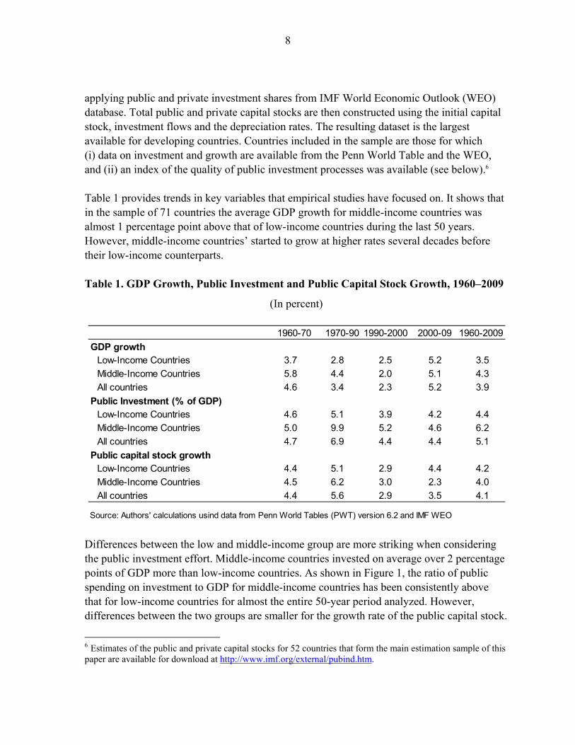
applying public and private investment shares from IMF World Economic Outlook (WEO) database. Total public and private capital stocks are then constructed using the initial capital stock, investment flows and the depreciation rates. The resulting dataset is the largest available for developing countries. Countries included in the sample are those for which (i) data on investment and growth are available from the Penn World Table and the WEO, and (ii) an index of the quality of public investment processes was available (see below).6 Table 1 provides trends in key variables that empirical studies have focused on. It shows that in the sample of 71 countries the average GDP growth for middle-income countries was almost 1 percentage point above that of low-income countries during the last 50 years. However, middle-income countries’ started to grow at higher rates several decades before their low-income counterparts. Table 1. GDP Growth, Public Investment and Public Capital Stock Growth, 1960–2009

(In percent)

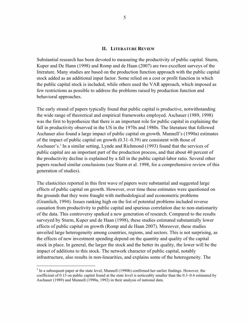
Differences between the low and middle-income group are more striking when considering the public investment effort. Middle-income countries invested on average over 2 percentage points of GDP more than low-income countries. As shown in Figure 1, the ratio of public spending on investment to GDP for middle-income countries has been consistently above that for low-income countries for almost the entire 50-year period analyzed. However, differences between the two groups are smaller for the growth rate of the public capital stock.

6 Estimates of the public and private capital stocks for 52 countries that form the main estimation sample of this paper are available for download at http://www.imf.org/external/pubind.htm.

1960-70 1970-90 1990-2000 2000-09 1960-2009

GDP growthLow-Income Countries 3.7 2.8 2.5 5.2 3.5

Middle-Income Countries 5.8 4.4 2.0 5.1 4.3

All countries 4.6 3.4 2.3 5.2 3.9

Public Investment (% of GDP)Low-Income Countries 4.6 5.1 3.9 4.2 4.4


All countries 4.7 6.9 4.4 4.4 5.1

Public capital stock growthLow-Income Countries 4.4 5.1 2.9 4.4 4.2


All countries 4.4 5.6 2.9 3.5 4.1

Source: Authors' calculations usind data from Penn World Tables (PWT) version 6.2 and IMF WEO

9

This could be attributable to the fact that a small addition to public capital can yield a large growth rate of the public capital stock when the level of capital is low (the base effect.)

Figure 1. Investment Ratio and Growth Rate of Public Capital

Sources: Penn World Table version 6.2, IMF WEO and authors’ calculations.

Serious data issues could undermine the quality of results on the productivity of public capital obtained from cross-country regressions. In particular, a large body of literature recognizes the importance of the quality and efficiency of public investment spending in determining the marginal productivity of investment. The real challenge in empirical research has been to find a good proxy for “efficiency-adjusted” public capital stock. To date, all empirical studies on the contribution of public capital to growth have assumed that public investment spending translates fully into productive capital assets. Several considerations can explain why cumulative public investment may not provide full information on growth of public capital. First, valuation issues make the measurement of any flows in a single currency problematic. Second, the cost of a given infrastructure asset can also vary significantly across countries, even after controlling for difference in conditions such as geology or geography. For example, the cost of building a road can be significantly higher in a country where procedures are not in place for project appraisal or where the environment is not conducive to competitive bidding. Third, weaknesses in the selection of the project could lead to an oversized project. The approach employed in this paper attempts to address these problems. In implementing this approach, we apply the methodology outlined by Pritchett (2000) to construct a new

MICs

LICs

24

68

10

1960 1970 1980 1990 2000 2010Year

(In percent)Average Growth Rate of Public Capital Stock

MICs

LICs4

68

1012

1960 1970 1980 1990 2000 2010Year

(In percent of GDP)Public Investment Ratio

10

public capital series that explicitly takes into account the efficiency of public investment. We measure the capital stock in country i and time period t as follows:

(2) ,

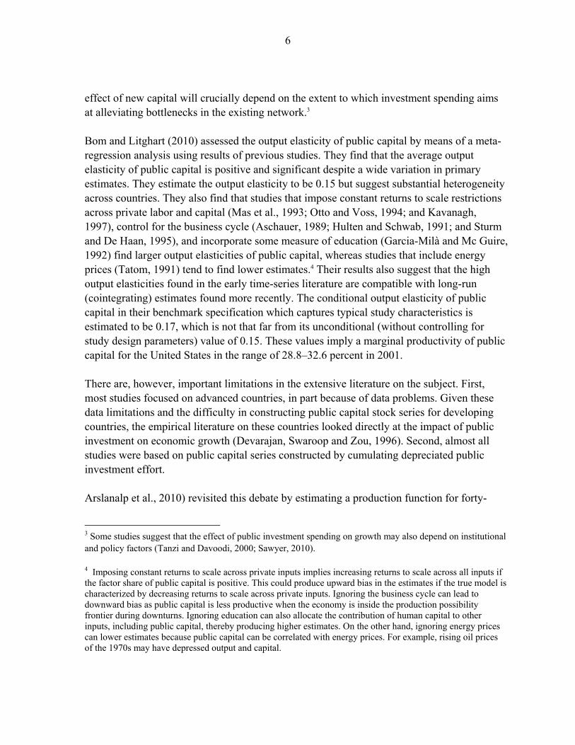
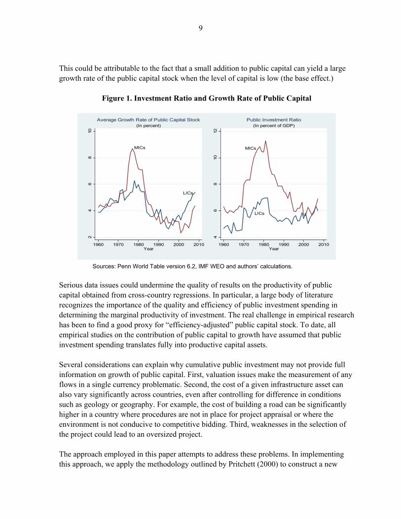
where is a time-invariant index that captures the efficiency of public investment. While the efficiency of investment processes is likely to evolve over time, it is also likely to change slowly reflecting the fact that structural reforms to improve these processes take time to implement. Thus we assume that is time-invariant. This index varies between 0, when all public resources are totally wasted, and 1, when full efficiency is achieved for government spending. However, we let this index vary in the robustness tests reported later in the paper. We use the normalized Public Investment Management Index (PIMI) as a proxy for ; the traditional perpetual inventory equation is a specific case of this more general formulation, where 1. PIMI is composed of 17 indicators grouped into four stages of the public investment management cycle: (i) Project Appraisal; (ii) Project Selection; (iii) Project Implementation; and (iv) Project Evaluation. In this index, countries are scored on the basis of different indicators and sub-indices, which are then combined to construct the overall index. The construction of the index relies upon an extensive data collection effort as described in Dabla-Norris et al. (2011).7 The sources largely cover the 2007–2010 periods, and include 71 countries (40 low-income countries and 31 middle-income countries).8 Table 2 suggests that, on average, in our set of countries only about half of public investment effort translates into actual productive public capital. This masks, however, significant heterogeneity between countries as illustrated in Figure 2. Beyond the large cross-country variation in overall scores described above, there is an even more notable variation for each of the sub-indices. This suggests that the observed differences in public investment management processes across countries stem largely from the substantial cross-country heterogeneity across the four stages of the investment process. To capture the variation across stages we also construct four alternative capital stock series for every country that correspond to three out of four investment stages (leaving one stage out) at a time. Estimation with these alternative series aim to identify which of the four public investment processes are the most important in capital accumulation and subsequently aggregate output. 7 Data were compiled from a large number of sources including from World Bank Public Investment Management case studies, Public Expenditure and Financial Accountability assessment reports, the Budget Institutions database, World Bank Public Expenditure Reviews, World Bank Country Procurement Assessment Reviews, World Bank Country Financial Accountability Assessments, and country websites. 8 The PIMI score is a simple average of the score for each stage of the public investment process. Countries with good investment processes have high scores. Scores for these stages are between 0 and 1 so that the total PIMI score is between 0 and 4 (for the full set of countries and country scores see Appendix A).

11

Table 2. Public Investment Management Index (PIMI) by Income Group

Figure 2. PIMI Distribution and Decomposition by Sub-Index

Source: Dabla-Norris et al. (2011) Note: For details see Dabla-Norris et al. (2011).

PIMI Appraisal Selection Implementation Evaluation

Low Income (40) 0.47 0.21 0.28 0.30 0.20(0.26) (0.13) (0.11) (0.10) (0.10)

Middle Income (31) 0.57 0.21 0.30 0.28 0.22(0.25) (0.09) (0.11) (0.07) (0.07)

All countries (71) 0.51 0.21 0.29 0.29 0.21(0.26) (0.11) (0.11) (0.09) (0.09)

Sources: Dabla-Norris et al. (2011) and authors' calculations. Standard deviations are in parentheses.

0

1

2

3

4

Belize

Co

ngo

, Rep

ub

lic of

Solo

mo

n Islan

ds

Yemen

West B

ank an

d G

azaSao

Tom

e and

Prin

cipe

Lao P

DR

Gam

bia

Bu

run

di

Togo

Senegal

Gab

on

Ch

adSierra Leo

ne

Sud

anH

aitiSw

aziland

Trinid

ad an

d To

bago

Gu

inea

Nigeria

Barb

ado

sD

jibo

uti

Tanzan

iaK

yrgyz Rep

ub

licEgyp

tU

gand

aIn

do

nesia

Ken

yaA

zerbaijan

Ben

inC

amb

od

iaP

akistanM

ozam

biq

ue

Alb

ania

Mo

nten

egroEth

iop

iaM

auritan

iaM

on

golia

Jamaica

Ko

sovo

El Salvado

rN

amib

iaM

alawi

Ph

ilipp

ines

Gh

ana

Co

te d'Ivo

ireZam

bia

Turkey

Lesoth

oFYR

Maced

on

iaU

kraine

Mad

agascar*Serb

iaB

anglad

eshB

elarus

Bu

rkina Faso

Afgh

anistan

Mali

Jord

anR

wan

da

Mo

ldo

vaB

otsw

ana

Kazakh

stanA

rmen

iaB

olivia

Peru

Thailan

dTu

nisia

Co

lom

bia

Brazil

Sou

th A

frica

Appraisal Selection Implementation Evaluation

Quartile 2 Quartile 3 Quartile 4Quartile 1

12

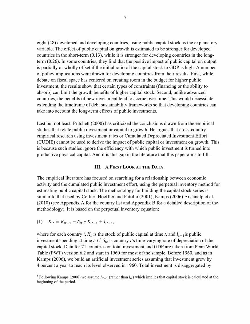
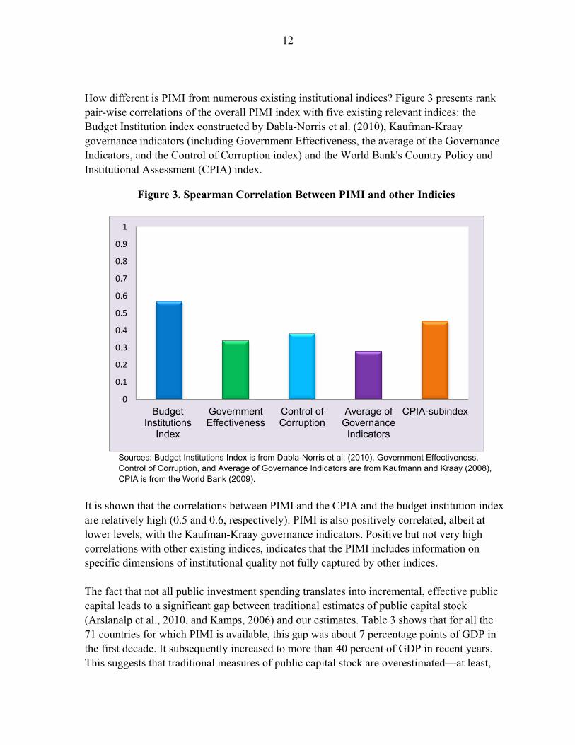
How different is PIMI from numerous existing institutional indices? Figure 3 presents rank pair-wise correlations of the overall PIMI index with five existing relevant indices: the Budget Institution index constructed by Dabla-Norris et al. (2010), Kaufman-Kraay governance indicators (including Government Effectiveness, the average of the Governance Indicators, and the Control of Corruption index) and the World Bank's Country Policy and Institutional Assessment (CPIA) index.

Figure 3. Spearman Correlation Between PIMI and other Indicies

Sources: Budget Institutions Index is from Dabla-Norris et al. (2010). Government Effectiveness, Control of Corruption, and Average of Governance Indicators are from Kaufmann and Kraay (2008), CPIA is from the World Bank (2009).

It is shown that the correlations between PIMI and the CPIA and the budget institution index are relatively high (0.5 and 0.6, respectively). PIMI is also positively correlated, albeit at lower levels, with the Kaufman-Kraay governance indicators. Positive but not very high correlations with other existing indices, indicates that the PIMI includes information on specific dimensions of institutional quality not fully captured by other indices. The fact that not all public investment spending translates into incremental, effective public capital leads to a significant gap between traditional estimates of public capital stock (Arslanalp et al., 2010, and Kamps, 2006) and our estimates. Table 3 shows that for all the 71 countries for which PIMI is available, this gap was about 7 percentage points of GDP in the first decade. It subsequently increased to more than 40 percent of GDP in recent years. This suggests that traditional measures of public capital stock are overestimated—at least,

0

0.1

0.2

0.3

0.4

0.5

0.6

0.7

0.8

0.9

1

Budget Institutions

Index

Government Effectiveness

Control of Corruption

Average of Governance Indicators

CPIA-subindex

13

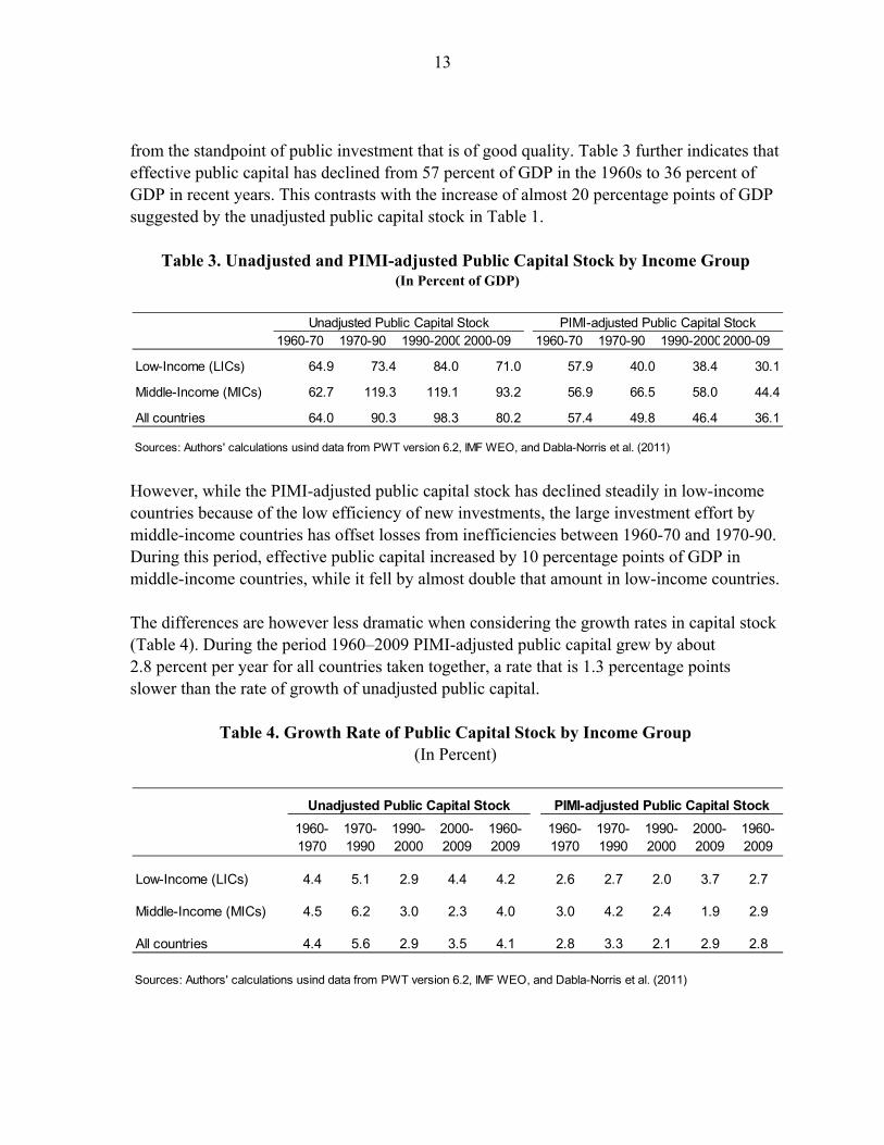
from the standpoint of public investment that is of good quality. Table 3 further indicates that effective public capital has declined from 57 percent of GDP in the 1960s to 36 percent of GDP in recent years. This contrasts with the increase of almost 20 percentage points of GDP suggested by the unadjusted public capital stock in Table 1.

Table 3. Unadjusted and PIMI-adjusted Public Capital Stock by Income Group (In Percent of GDP)

However, while the PIMI-adjusted public capital stock has declined steadily in low-income countries because of the low efficiency of new investments, the large investment effort by middle-income countries has offset losses from inefficiencies between 1960-70 and 1970-90. During this period, effective public capital increased by 10 percentage points of GDP in middle-income countries, while it fell by almost double that amount in low-income countries. The differences are however less dramatic when considering the growth rates in capital stock (Table 4). During the period 1960–2009 PIMI-adjusted public capital grew by about 2.8 percent per year for all countries taken together, a rate that is 1.3 percentage points slower than the rate of growth of unadjusted public capital.

Table 4. Growth Rate of Public Capital Stock by Income Group (In Percent)

1960-70 1970-90 1990-20002000-09 1960-70 1970-90 1990-20002000-09

Low-Income (LICs) 64.9 73.4 84.0 71.0 57.9 40.0 38.4 30.1

Middle-Income (MICs) 62.7 119.3 119.1 93.2 56.9 66.5 58.0 44.4

All countries 64.0 90.3 98.3 80.2 57.4 49.8 46.4 36.1

Sources: Authors' calculations usind data from PWT version 6.2, IMF WEO, and Dabla-Norris et al. (2011)

Unadjusted Public Capital Stock PIMI-adjusted Public Capital Stock

1960-1970

1970-1990

1990-2000

2000-2009

1960-2009

1960-1970

1970-1990

1990-2000

2000-2009

1960-2009

Low-Income (LICs) 4.4 5.1 2.9 4.4 4.2 2.6 2.7 2.0 3.7 2.7

Middle-Income (MICs) 4.5 6.2 3.0 2.3 4.0 3.0 4.2 2.4 1.9 2.9

All countries 4.4 5.6 2.9 3.5 4.1 2.8 3.3 2.1 2.9 2.8

Sources: Authors' calculations usind data from PWT version 6.2, IMF WEO, and Dabla-Norris et al. (2011)

Unadjusted Public Capital Stock PIMI-adjusted Public Capital Stock

14

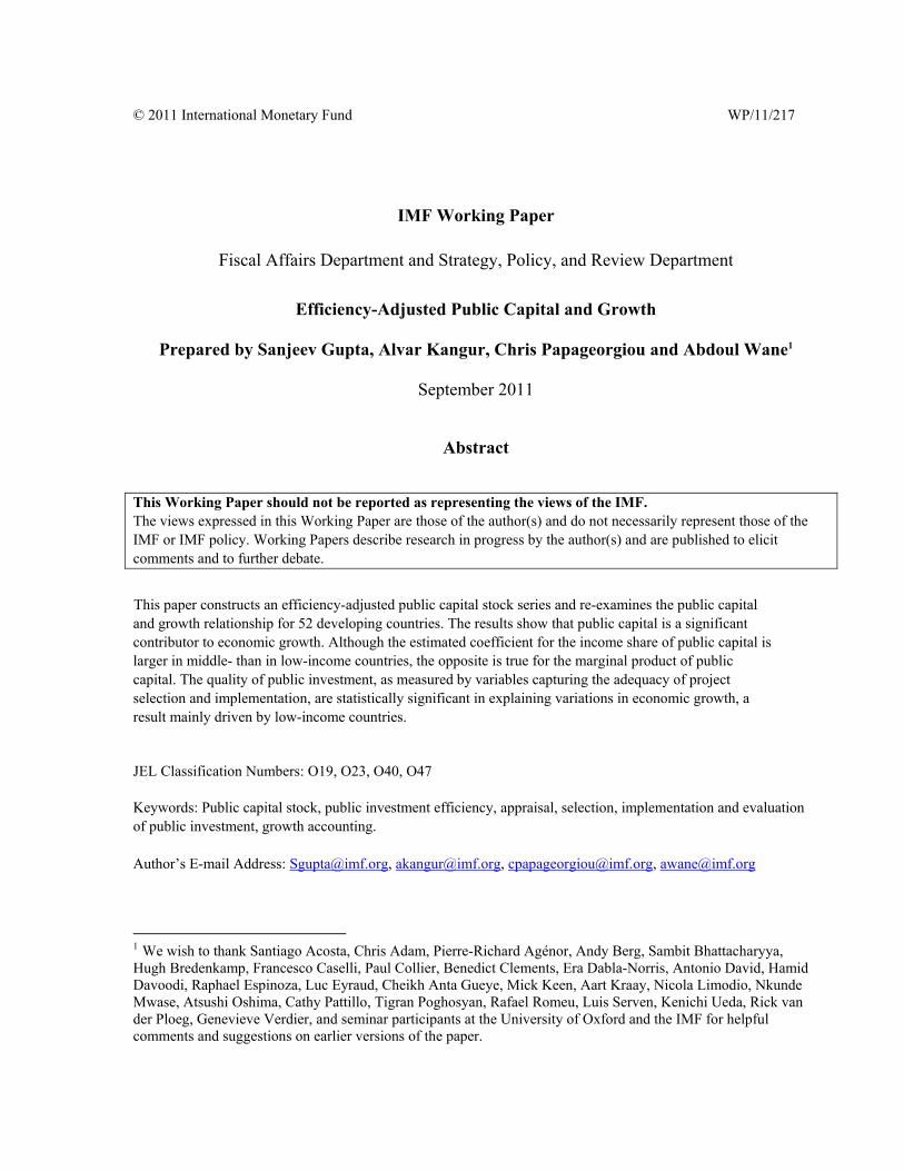
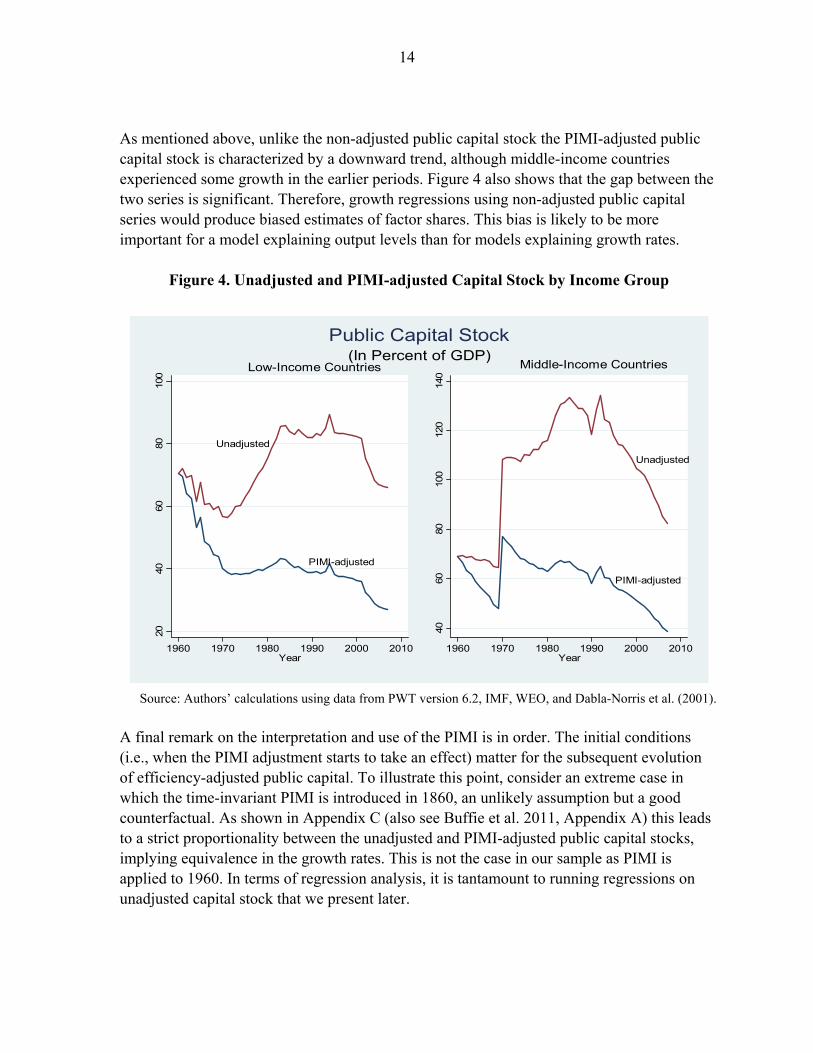
As mentioned above, unlike the non-adjusted public capital stock the PIMI-adjusted public capital stock is characterized by a downward trend, although middle-income countries experienced some growth in the earlier periods. Figure 4 also shows that the gap between the two series is significant. Therefore, growth regressions using non-adjusted public capital series would produce biased estimates of factor shares. This bias is likely to be more important for a model explaining output levels than for models explaining growth rates.

Figure 4. Unadjusted and PIMI-adjusted Capital Stock by Income Group

Source: Authors’ calculations using data from PWT version 6.2, IMF, WEO, and Dabla-Norris et al. (2001).

A final remark on the interpretation and use of the PIMI is in order. The initial conditions (i.e., when the PIMI adjustment starts to take an effect) matter for the subsequent evolution of efficiency-adjusted public capital. To illustrate this point, consider an extreme case in which the time-invariant PIMI is introduced in 1860, an unlikely assumption but a good counterfactual. As shown in Appendix C (also see Buffie et al. 2011, Appendix A) this leads to a strict proportionality between the unadjusted and PIMI-adjusted public capital stocks, implying equivalence in the growth rates. This is not the case in our sample as PIMI is applied to 1960. In terms of regression analysis, it is tantamount to running regressions on unadjusted capital stock that we present later.

Low-Income Countries

Unadjusted

PIMI-adjusted

2040

6080

100

1960 1970 1980 1990 2000 2010Year

Middle-Income Countries

Unadjusted

PIMI-adjusted

4060

8010

012

014

0

1960 1970 1980 1990 2000 2010Year

(In Percent of GDP)Public Capital Stock

15

IV. PUBLIC CAPITAL AND GROWTH: PANEL REGRESSION ANALYSIS

A. Estimation Method

We use the production function approach to estimate the contribution of public capital to growth. The production function is specified as:

(3) , , , where Yt is the real aggregate level of output (GDP) at period t, Kt is the aggregate private capital stock, Gt is the aggregate public capital stock, and St is skill-adjusted aggregate labor supply. This represents an additional deviation of our analysis from existing work: rather than using raw labor, we construct and use skill-adjusted labor incorporating data on average years on education. Following the literature on returns to education St is computed according to S L e , where Lit is raw labor and h is the average years of schooling in the population aged 15 years and older. φ(h) is a stepwise linear function adjusting the average years of schooling by estimates for returns on education. Assuming Cobb-Douglas production function technology, A, α, β and γ are parameters satisfying A > 0, and α, β, γ (0, 1).9 We begin our empirical analysis by specifying the aggregate input-output production relationship:

(4) ,

where A0 denotes the initial (1960) value of the scale factor, i is a country identification, and we assume year-specific intercepts λt that could reflect common (Hicks-neutral) exogenous technology shocks.

Taking logarithms of both sides gives us: (5) .

Admitting the possibility of country-specific effects implies that the error term in (5) can be written as εit = ηi + υit, where ηi captures time-invariant fixed factors in country i and υit captures the omitted factors. Traditional approach to estimation is to difference this equation 9 In the robustness analysis, we also consider the more flexible CES aggregate production function specification.

16

to yield 5-year average growth rates in the respective variables. This would eliminate fixed effects, thus controlling for any country-specific but time-invariant characteristic (such as colonial legacies, legal origins, ethnic fragmentation, etc.) that could affect both the capital stocks and per capita income growth. The reasons for using 5-year, rather than annual frequency data are twofold: first, it mitigates business-cycle effects and second, it allows us to capture investment in human capital by using Barro and Lee (2010) data, which are available as five-year averages. While it is straightforward to estimate (5) using a panel estimation that incorporates country fixed effects (to purge individual growth effects) as well as time effects, concerns regarding simultaneity still remain. Many authors argue that public capital itself is an endogenous variable due to feedback from income-savings decision on capital accumulation.10 A traditional approach to deal with this problem would be to use lagged levels to instrument for differences. However, if the underlying series are close to a unit root (which is usually the case with macro-variables such as public capital), past levels contain little or no information about future changes and are thus weak instruments. To address this issue we chose to use a system Generalized Method of Moments (GMM) (Blundell and Bond, 1998) estimator.11 In addition, in the GMM estimation strategy, we allow for an AR(1) component in the idiosyncratic shock υit, of the form υ = ρυ that Blundell and Bond (2000) have found important in obtaining valid instruments. This leads to a dynamic (common factor) representation of equation (3) of the form:12 (6)

1 1 .

10 The first-difference specification further magnifies this problem; even if independent variables are predetermined, in the first-differenced equation their time t values are likely to be correlated with the lagged error term, υit-1. More generally, the capital accumulation equation used to construct the capital stock series (see the data appendix for details) implies that Kit will depend on such lagged error terms. Therefore, instrumental variables are needed to correct for endogeneity.

11 This approach permits us to transform the instruments to make them orthogonal to the fixed effects.

12 This dynamic representation implies three non-linear (common factor) restrictions on the unrestricted parameters that generally hold in the baseline regressions. To save space the lagged terms are compressed in the presentation of the estimation results. This form incorporates the traditional dynamic panel endogeneity bias that we address with system GMM internal instruments. We assume that all factors of production (Kit, Git, Sit) are potentially contemporaneously correlated with the country specific effects (ηi) as well as idiosyncratic shocks (ϵit).

17

B. Results

Our empirical analysis is organized in two parts: First, we present baseline results that include estimation of the contribution of the overall PIMI-adjusted public capital stock to growth, and also the contribution of different stages of the public investment process to the efficiency of capital and growth. Second, we present numerous robustness tests for alternative specifications, econometric approaches and samples. The sample size is reduced to 52 because of missing observations for some countries.

C. Baseline Results

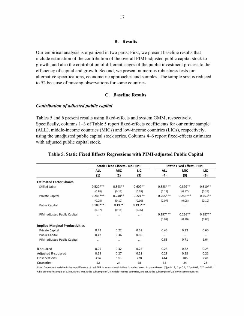
Contribution of adjusted public capital Tables 5 and 6 present results using fixed-effects and system GMM, respectively. Specifically, columns 1–3 of Table 5 report fixed-effects coefficients for our entire sample (ALL), middle-income countries (MICs) and low-income countries (LICs), respectively, using the unadjusted public capital stock series. Columns 4–6 report fixed-effects estimates with adjusted public capital stock.

Table 5. Static Fixed Effects Regressions with PIMI-adjusted Public Capital

ALL MIC LIC ALL MIC LIC

(1) (2) (3) (4) (5) (6)

Estimated Factor Shares

Skilled Labor 0.522*** 0.393** 0.602** 0.523*** 0.399** 0.610**

(0.18) (0.17) (0.29) (0.19) (0.17) (0.29)

Private Capital 0.245*** 0.248** 0.221** 0.265*** 0.258*** 0.253**

(0.08) (0.10) (0.10) (0.07) (0.08) (0.10)

Public Capital 0.189*** 0.197* 0.193*** … … …

(0.07) (0.11) (0.06)

PIMI-adjusted Public Capital … … … 0.197*** 0.226** 0.187**

(0.07) (0.10) (0.08)

Implied Marginal Productivities

Private Capital 0.42 0.22 0.52 0.45 0.23 0.60

Public Capital 0.42 0.36 0.50 … … …

PIMI-adjusted Public Capital … … … 0.88 0.71 1.04

R-squared 0.25 0.32 0.25 0.25 0.32 0.25

Adjusted R-squared 0.23 0.27 0.21 0.23 0.28 0.21

Observations 414 186 228 414 186 228

Countries 52 24 28 52 24 28

Note: Dependent variable is the log-difference of real GDP in international dollars. Standard errors in parentheses: [*] p<0.15, * p<0.1, ** p<0.05, *** p<0.01.

All is our entire sample of 52 countries, MIC is the subsample of 24 middle-income countries, and LIC is the subsample of 28 low-income countries

Static Fixed Effects - No PIMI Static Fixed Effect - PIMI

18

Table 6. Dynamic System GMM Regressions with PIMI-adjusted Public Capital

Comparing the fixed-effects models’ results using “unadjusted” public capital stocks with efficiency-adjusted capital shows that coefficient estimates for private and efficiency-adjusted public capital increase somewhat (except in the LIC subsample, where the coefficient of efficiency-adjusted public capital decreases slightly). Perhaps more importantly, this comparison shows that using raw public capital leads to underestimating the contribution of private capital inputs. Under the panel fixed-effects specification with PIMI-adjusted capital, all coefficient estimates are significant at least at the 5 percent level. The unconstrained factor share estimates for the entire sample of counties (ALL; column 4) are 52.3 percent for skilled labor, 26.5 percent for private capital and 19.7 percent of for public capital. This contribution of public capital is consistent with the finding by Bom and Litghart (2010). Our estimate is higher than the unconditional average they report (15 percent), but this could result from the inclusion of a measure of education in our production function.

ALL MIC LIC ALL MIC LIC

(1) (2) (3) (4) (5) (6)


Skilled Labor 0.390** 0.265* 0.583*** 0.336* 0.249* 0.637***

(0.18) (0.14) (0.22) (0.19) (0.15) (0.23)

Private Capital 0.231** 0.286*** 0.231** 0.297*** 0.314*** 0.300***

(0.09) (0.10) (0.09) (0.09) (0.10) (0.09)

Public Capital 0.233*** 0.167** 0.253*** … … …

(0.07) (0.08) (0.09)

PIMI-adjusted Public Capital … … … 0.154* 0.162** 0.143*

(0.08) (0.07) (0.09)


Private Capital 0.40 0.26 0.55 0.51 0.28 0.71

Public Capital 0.52 0.30 0.65 … … …

PIMI-adjusted Public Capital … … … 0.69 0.51 0.80

Hansen J-test [1.00] [1.00] [1.00] [1.00] [1.00] [1.00]

AR(2) test [0.71] [0.51] [0.77] [0.60] [0.50] [0.86]

Common factors [0.13] [0.04] [0.64] [0.14] [0.09] [0.75]

Observations 414 186 228 414 186 228

Countries 52 24 28 52 24 28



Dynamic GMM - No PIMI Dynamic GMM - PIMI

19

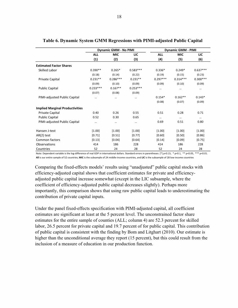
Although the fixed-effect results may provide a comparison with many existing studies, our preferred specification is dynamic system-GMM that corrects for endogeneity (Table 6).13 The coefficient estimates for adjusted public capital are now notably smaller in magnitude compared to those for unadjusted public capital, dropping from 0.23 to 0.15 for the entire sample. This is driven by LICs where factor share of public capital falls from 0.25 to 0.14, while for MICs estimated coefficients are almost the same. All coefficient estimates retain their significance at least at 10 percent significance level. Interestingly, coefficient estimates for private capital show a corresponding increase in all samples that is much larger in magnitude than in case of fixed effects. For example, for ALL and LIC samples the estimated coefficients increase from 0.23 to 0.3, while for the MIC sample there is a more modest increase from 0.29 to 0.31. Table 6 (columns 4-6) also shows that there is an almost twofold difference between adjusted public and private capital in all three samples (around 15 percent for public capital and 30 percent for private capital). Tables 5 and 6 present calculations of respective marginal product of factors defined as MPX =a(Y/X), where a is the income factor share, Y is GDP and X(S, K, G). For public capital MPG = β(GDP/GPIMI). Focusing on MPG under the fixed effect model (Table 5) it is shownthat for the entire sample there is large jump from 0.42 to 0.88 after correcting the capital series for public investment inefficiencies. This is not unexpected given that the modified Y/G ratio in the MPG equation increases substantially and especially for LICs. Under the dynamic GMM model this jump is smaller but still quite significant from 0.52 to 0.69. These results highlight that although the income share of public capital is low (only 14 percent for LICs), the MPG is high given downward corrections in the public capital series to capture inefficiencies.

Overall, this result suggests that ignoring public investment inefficiencies leads to an underestimation of marginal productivities of both private and public capital, which can have important policy implications. Furthermore, the marginal productivity of public capital is only slightly larger than that of private capital when public investment inefficiencies are ignored. However, once public investment inefficiencies are corrected for, the absolute gap between the productivities of public and private capital widens.14 It is also noteworthy that the regressions with

13 Table 6 also reports p-values from joint tests of the common factor restrictions implied by our dynamic equation (6). The common factors are marginally rejected at 10 percent only for the MICs subsample, however, closer inspection revealed that this is related to somewhat underestimated factor share of skilled labor (in PWT labor is based on working-age population and might not properly capture variations in hours worked). Imposing constant returns to scale would increase the labor share and yield a p-value of 0.42, thus supporting the validity of restrictions.

14 A cautionary remark is in place here. Our estimation of marginal products is based on how the PIMI adjustment affects the physical marginal product of capital and not the financial (price-adjusted) marginal product of capital as in Caselli and Feyrer (2007).

20

efficiency adjusted public capital seem to better explain the variation in output. Although standard goodness of fit measures are not readily available for GMM, regressions with PIMI-adjusted public capital show lower error variance and more than 11 percent reduction in the mean-squared-errors of predicted output levels.

Contribution of investment processes

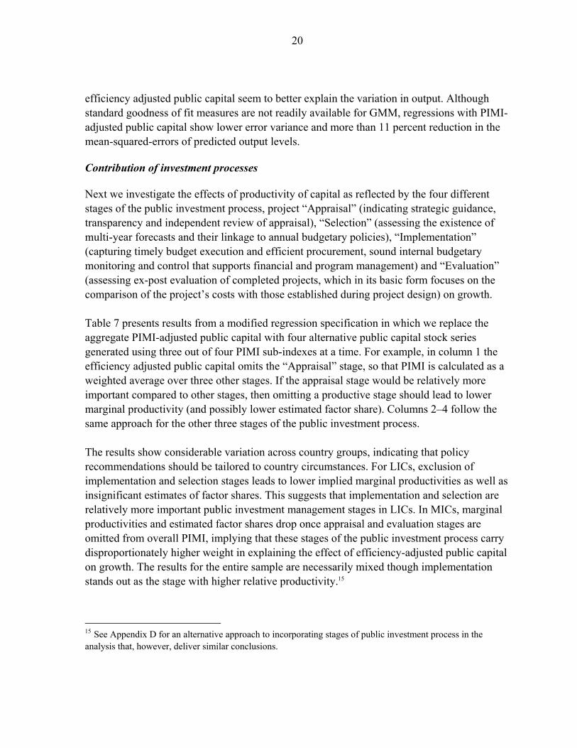
Next we investigate the effects of productivity of capital as reflected by the four different stages of the public investment process, project “Appraisal” (indicating strategic guidance, transparency and independent review of appraisal), “Selection” (assessing the existence of multi-year forecasts and their linkage to annual budgetary policies), “Implementation” (capturing timely budget execution and efficient procurement, sound internal budgetary monitoring and control that supports financial and program management) and “Evaluation” (assessing ex-post evaluation of completed projects, which in its basic form focuses on the comparison of the project’s costs with those established during project design) on growth. Table 7 presents results from a modified regression specification in which we replace the aggregate PIMI-adjusted public capital with four alternative public capital stock series generated using three out of four PIMI sub-indexes at a time. For example, in column 1 the efficiency adjusted public capital omits the “Appraisal” stage, so that PIMI is calculated as a weighted average over three other stages. If the appraisal stage would be relatively more important compared to other stages, then omitting a productive stage should lead to lower marginal productivity (and possibly lower estimated factor share). Columns 2–4 follow the same approach for the other three stages of the public investment process. The results show considerable variation across country groups, indicating that policy recommendations should be tailored to country circumstances. For LICs, exclusion of implementation and selection stages leads to lower implied marginal productivities as well as insignificant estimates of factor shares. This suggests that implementation and selection are relatively more important public investment management stages in LICs. In MICs, marginal productivities and estimated factor shares drop once appraisal and evaluation stages are omitted from overall PIMI, implying that these stages of the public investment process carry disproportionately higher weight in explaining the effect of efficiency-adjusted public capital on growth. The results for the entire sample are necessarily mixed though implementation stands out as the stage with higher relative productivity.15

15 See Appendix D for an alternative approach to incorporating stages of public investment process in the analysis that, however, deliver similar conclusions.

21

Table 7. Regressions for Public Investment Stage

Omitted category: Appraisal Selection mplementation Evaluation Appraisal Selection mplementation Evaluation Appraisal Selection mplementation Evaluation

(1) (2) (3) (4) (1) (2) (3) (4) (1) (2) (3) (4)


Skilled Labor 0.327* 0.322* 0.360* 0.348* 0.260* 0.234[*] 0.242* 0.265* 0.649*** 0.637*** 0.647*** 0.620***

(0.19) (0.19) (0.19) (0.19) (0.15) (0.15) (0.14) (0.16) (0.23) (0.23) (0.23) (0.22)

Private Capital 0.290*** 0.297*** 0.307*** 0.299*** 0.320*** 0.329*** 0.296*** 0.314*** 0.294*** 0.302*** 0.312*** 0.303***

(0.09) (0.09) (0.09) (0.09) (0.10) (0.09) (0.09) (0.10) (0.10) (0.10) (0.09) (0.09)

PIMI-adjusted Public Capital 0.154* 0.157* 0.143* 0.158* 0.155** 0.166*** 0.183*** 0.155** 0.149[*] 0.133 0.122 0.152*

(0.08) (0.08) (0.09) (0.08) (0.07) (0.06) (0.06) (0.07) (0.10) (0.09) (0.09) (0.08)


Private Capital 0.496 0.508 0.525 0.512 0.290 0.298 0.268 0.284 0.696 0.715 0.739 0.718

PIMI-adjusted Public Capital 0.680 0.753 0.665 0.674 0.474 0.551 0.591 0.467 0.822 0.798 0.709 0.803

Hansen J-test [1.00] [1.00] [1.00] [1.00] [1.00] [1.00] [1.00] [1.00] [1.00] [1.00] [1.00] [1.00]

AR(2) test [0.61] [0.59] [0.59] [0.61] [0.50] [0.50] [0.51] [0.49] [0.84] [0.88] [0.88] [0.85]

Common factors [0.10] [0.14] [0.20] [0.14] [0.08] [0.13] [0.09] [0.07] [0.55] [0.83] [0.88] [0.78]

Observations 414 414 414 414 186 186 186 186 228 228 228 228

Countries 52 52 52 52 24 24 24 24 28 28 28 28



Dynamic GMM: ALL Dynamic GMM: MIC Dynamic GMM: LIC

22

0.0

0.2

0.4

0.6

0.8

1.0

1985 1990 1995 2000 2005 2010

Figure 5. Time-varying PIMI (normalized)

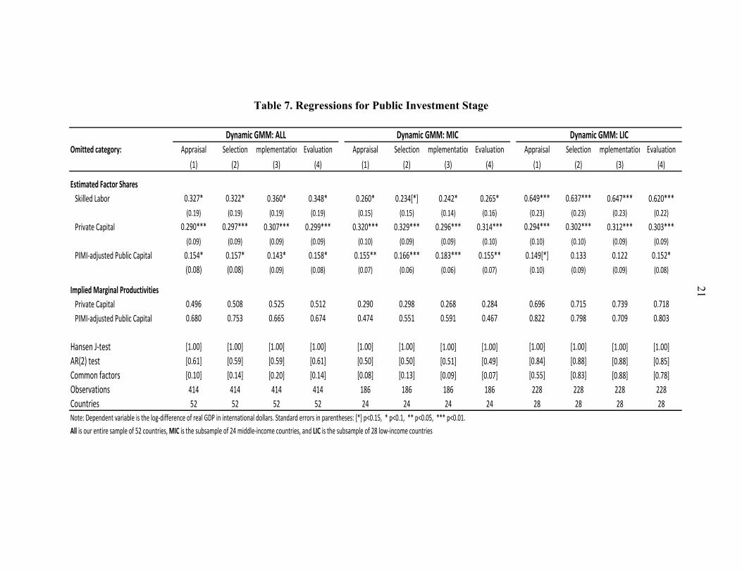
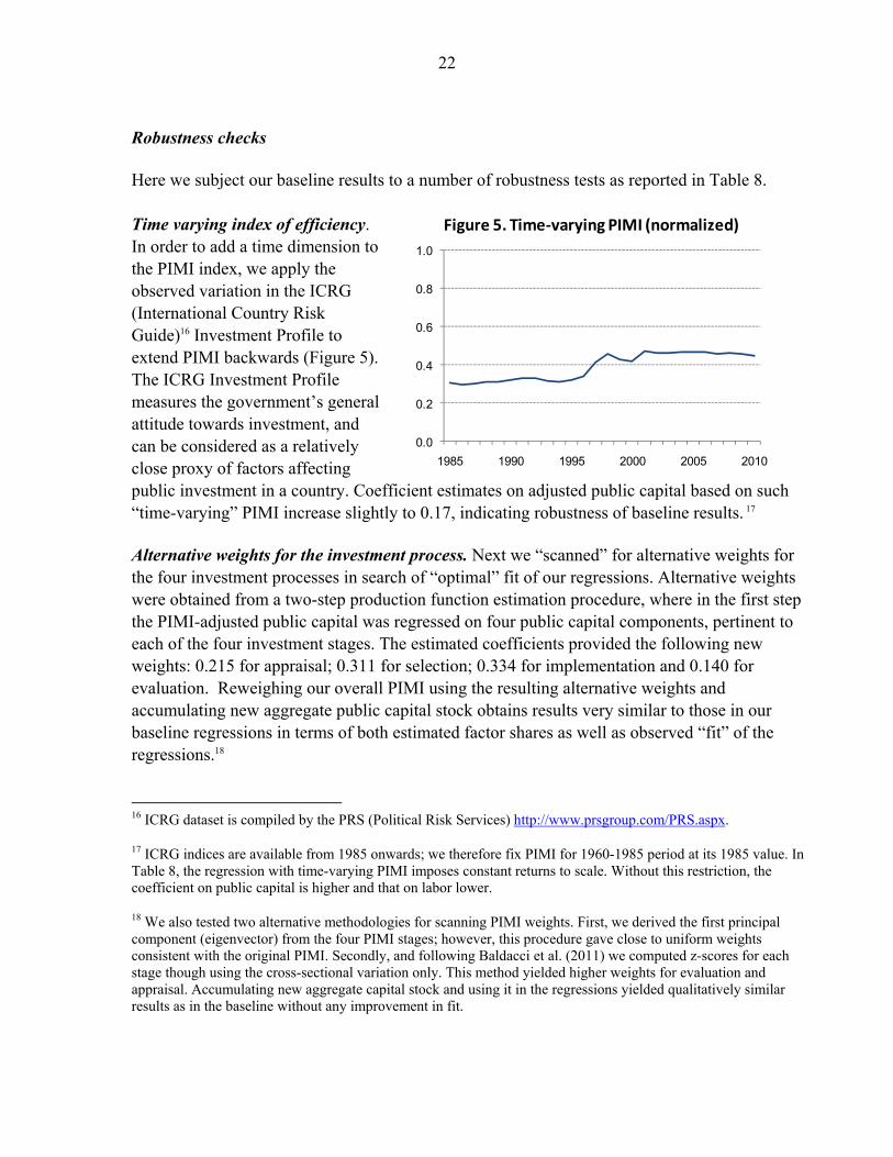
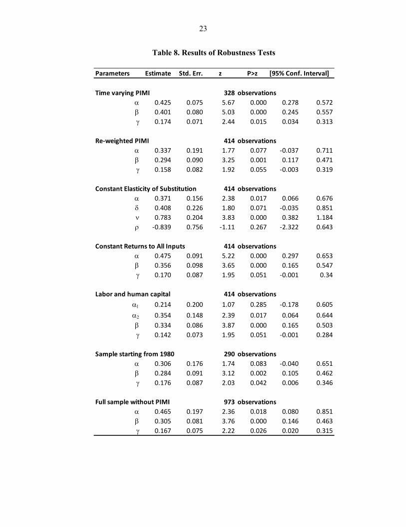
Robustness checks Here we subject our baseline results to a number of robustness tests as reported in Table 8. Time varying index of efficiency. In order to add a time dimension to the PIMI index, we apply the observed variation in the ICRG (International Country Risk Guide)16 Investment Profile to extend PIMI backwards (Figure 5). The ICRG Investment Profile measures the government’s general attitude towards investment, and can be considered as a relatively close proxy of factors affecting public investment in a country. Coefficient estimates on adjusted public capital based on such “time-varying” PIMI increase slightly to 0.17, indicating robustness of baseline results. 17 Alternative weights for the investment process. Next we “scanned” for alternative weights for the four investment processes in search of “optimal” fit of our regressions. Alternative weights were obtained from a two-step production function estimation procedure, where in the first step the PIMI-adjusted public capital was regressed on four public capital components, pertinent to each of the four investment stages. The estimated coefficients provided the following new weights: 0.215 for appraisal; 0.311 for selection; 0.334 for implementation and 0.140 for evaluation. Reweighing our overall PIMI using the resulting alternative weights and accumulating new aggregate public capital stock obtains results very similar to those in our baseline regressions in terms of both estimated factor shares as well as observed “fit” of the regressions.18

16 ICRG dataset is compiled by the PRS (Political Risk Services) http://www.prsgroup.com/PRS.aspx.

17 ICRG indices are available from 1985 onwards; we therefore fix PIMI for 1960-1985 period at its 1985 value. In Table 8, the regression with time-varying PIMI imposes constant returns to scale. Without this restriction, the coefficient on public capital is higher and that on labor lower.

18 We also tested two alternative methodologies for scanning PIMI weights. First, we derived the first principal component (eigenvector) from the four PIMI stages; however, this procedure gave close to uniform weights consistent with the original PIMI. Secondly, and following Baldacci et al. (2011) we computed z-scores for each stage though using the cross-sectional variation only. This method yielded higher weights for evaluation and appraisal. Accumulating new aggregate capital stock and using it in the regressions yielded qualitatively similar results as in the baseline without any improvement in fit.

23

Table 8. Results of Robustness Tests

Parameters Estimate Std. Err. z P>z Interval]

328

0.425 0.075 5.67 0.000 0.278

0.401 0.080 5.03 0.000 0.245

0.174 0.071 2.44 0.015 0.034

414

0.337 0.191 1.77 0.077 -0.037

0.294 0.090 3.25 0.001 0.117

0.158 0.082 1.92 0.055 -0.003

414

0.371 0.156 2.38 0.017 0.066

0.408 0.226 1.80 0.071 -0.035

0.783 0.204 3.83 0.000 0.382

-0.839 0.756 -1.11 0.267 -2.322

414

0.475 0.091 5.22 0.000 0.297

0.356 0.098 3.65 0.000 0.165

0.170 0.087 1.95 0.051 -0.001

414

0.214 0.200 1.07 0.285 -0.178

0.354 0.148 2.39 0.017 0.064

0.334 0.086 3.87 0.000 0.165

0.142 0.073 1.95 0.051 -0.001

290

0.306 0.176 1.74 0.083 -0.040

0.284 0.091 3.12 0.002 0.105

0.176 0.087 2.03 0.042 0.006

973

0.465 0.197 2.36 0.018 0.080

0.305 0.081 3.76 0.000 0.146

0.167 0.075 2.22 0.026 0.020

0.313

Constant Returns to All Inputs observations

0.676

[95% Conf.

Constant Elasticity of Substitution observations

0.711

0.471

0.319

Time varying PIMI observations

0.572

Re-weighted PIMI observations

0.557

Sample starting from 1980 observations

0.651

0.462

0.503

0.284

observations

0.605

0.644

0.653

0.547

0.34

Labor and human capital observations

0.851

1.184

0.643

0.851

0.463

0.315

0.346

Full sample without PIMI

24

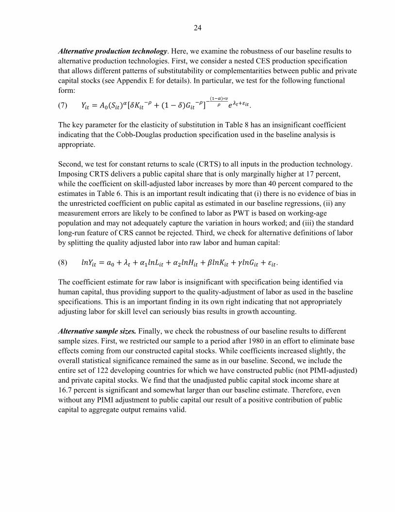
Alternative production technology. Here, we examine the robustness of our baseline results to alternative production technologies. First, we consider a nested CES production specification that allows different patterns of substitutability or complementarities between public and private capital stocks (see Appendix E for details). In particular, we test for the following functional form:

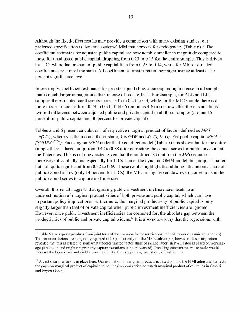
(7) 1 . The key parameter for the elasticity of substitution in Table 8 has an insignificant coefficient indicating that the Cobb-Douglas production specification used in the baseline analysis is appropriate. Second, we test for constant returns to scale (CRTS) to all inputs in the production technology. Imposing CRTS delivers a public capital share that is only marginally higher at 17 percent, while the coefficient on skill-adjusted labor increases by more than 40 percent compared to the estimates in Table 6. This is an important result indicating that (i) there is no evidence of bias in the unrestricted coefficient on public capital as estimated in our baseline regressions, (ii) any measurement errors are likely to be confined to labor as PWT is based on working-age population and may not adequately capture the variation in hours worked; and (iii) the standard long-run feature of CRS cannot be rejected. Third, we check for alternative definitions of labor by splitting the quality adjusted labor into raw labor and human capital: (8) . The coefficient estimate for raw labor is insignificant with specification being identified via human capital, thus providing support to the quality-adjustment of labor as used in the baseline specifications. This is an important finding in its own right indicating that not appropriately adjusting labor for skill level can seriously bias results in growth accounting. Alternative sample sizes. Finally, we check the robustness of our baseline results to different sample sizes. First, we restricted our sample to a period after 1980 in an effort to eliminate base effects coming from our constructed capital stocks. While coefficients increased slightly, the overall statistical significance remained the same as in our baseline. Second, we include the entire set of 122 developing countries for which we have constructed public (not PIMI-adjusted) and private capital stocks. We find that the unadjusted public capital stock income share at 16.7 percent is significant and somewhat larger than our baseline estimate. Therefore, even without any PIMI adjustment to public capital our result of a positive contribution of public capital to aggregate output remains valid.

25

V. CONCLUDING REMARKS

This paper makes three contributions to the existing literature that investigates the contribution of public capital to growth. First, it constructed a new dataset on private and public capital in which public capital takes into account public investment inefficiencies. Controlling for these inefficiencies showed that the actual accumulation of productive public capital was significantly slower than suggested by government spending on investment. Our results suggest that the stock of effective public capital might be up to one-half of the stock suggested by the traditional method for computing public capital stock. Second, we provided further evidence in favor of a significant role for public capital in explaining output variations. Our baseline specification as well as alternative robustness specifications showed a consistently significant impact of public capital on output. We find that the productivity of public capital has been grossly underestimated by the previous studies. Moreover, our study indicated that the productivity of public capital, controlling for the efficiency of investment processes, is significantly higher than the marginal cost of funds under normal financing conditions. This is especially true for LICs. Finally, our results suggest that project implementation is the most important component of the overall investment process. This result is driven by LICs followed by project selection. Thus improving project implementation comprising competitive bidding and internal audit, and project selection, comprising existence of MT frameworks and their linkage to annual budgetary policies, can significantly benefit public investment and growth in low-income countries. The recommendations for strengthening public investment processes would, however, need to be tailored to country circumstances, given that in MICs it is project appraisal and evaluation that are found to be relatively more productive stages.

26

References

Agénor, P.-R., 2009, “Infrastructure Investment and Maintenance Expenditure: Optimal Allocation Rules in a Growing Economy,” Journal of Public Economic Theory 11, pp. 233–50.

Agénor, P.-R., 2010, “A Theory of Infrastructure-Led Development,” Journal of Economic Dynamics and Control 34, pp. 932–50.

Arslanalp S., F. Bonhorst, S. Gupta, and E. Sze (2010), “Public Capital and Growth,” IMF Working Paper 10/175.

Aschauer, D. A., 1989, “Is Public Expenditure Productive?” Journal of Monetary Economics 23, pp. 177–200.

Aschauer, D. A., 1998, “How Big Should the Public Capital Stock Be?” The Jerome Levy Economics Institute of Bard College Public Policy, No: 43.

Baldacci, E., J. McHugh, and I. Petrova, 2011, “Measuring Fiscal Vulnerability and Fiscal Stress: A Proposed Set of Indicators,” IMF Working Paper 11/94 (Washington: International Monetary Fund).

Barro, R., and J.-W. Lee, 2010, “A New Data Set of Educational Attainment in the World, 1950–2010,” NBER Working Paper No. 15902.

Blundell, R., and S. Bond, 1998, “Initial Conditions and Moment Restrictions in Dynamic Panel Data Models,” Journal of Econometrics 87, pp. 115–43.

Blundell, R., and S. Bond, 2000, “GMM Estimation with Persistent Panel Data: An Application to Production Functions,” Econometric Reviews 19, pp. 321–40.

Bom, P., and J. E. Ligthart, 2010, “What Have We Learned From Three Decades of Research on the Productivity of Public Capital?,” CESifo Working Paper Series No. 2206, Center Discussion Paper No. 2008–10.

Buffie E., A. Berg, C. Pattillo, R. Portillo, and L.F. Zanna, 2011, “Public Investment, Growth and Debt Sustainability: Putting Together the Pieces,” draft paper, IMF.

Collier, P., A. Hoeffler, and C. Pattillo, 2001, “Flight Capital as a Portfolio Choice,” The World Bank Economic Review 15, pp. 55–80.

Dabla-Norris, E., Brumby, J., Kyobe, A., Mills, Z., and Chris Papageorgiou, 2011, “Investing in Public Investment: An Index of Public Investment Efficiency,” IMF Working Paper 11/37 (Washington: International Monetary Fund).

Dabla-Norris, E., Allen, R., Zanna, L-F., Prakash, T., Kvintradze, E. Lledo, V., Yackovlev, I. and Gollwitzer, S., 2009, “Budget Institutions and Fiscal Performance in Low-Income Countries,” IMF Working Paper 10/80 (Washington: International Monetary Fund).

27

Devarajan, S., V. Swaroop, and H. F. Zou, 1996, “The Composition of Public Expenditure and Economic Growth,” Journal of Monetary Economics 37, 313–144.

Garcia-Mila, T., and T. J. McGuire, 1992, “The Contribution of Publicly Provided Inputs to States' Economies,” Regional Science and Urban Economics 22, 229–41.

Hulten, C. R., and R. M. Schwab, 1991, “Is There Too Little Public Capital: Infrastructure and Economic Growth,” Conference paper, American Enterprise Institute, Washington, DC.

International Monetary Fund, 2009, “The Fund’s Facilities and Financing Framework for Low-Income Countries,” SM/09/55, SM/09/55 Supplement 1, SM/09/55 Supplement2, (Washington: International Monetary Fund).

Isham, J., D. Narayan, and L. Pritcett, 1995, “Does Participation Improve Performance? Establishing Causality with Subjective Data,” The World Bank Economic Review 9, pp. 175–200.

Johnson, S., W. Larson, C. Papageorgiou, and A. Subramanian, 2009, “Is Newer Better? Penn

World Table Revisions and Their Impact on Growth Estimates,” NBER Working Paper No. 15455.

Kamps, C., 2006, “New Estimates of Government Net Capital Stocks for 22 OECD Countries, 1960–2001,” IMF Staff Papers 53, pp. 120–50.

Kaufmann, D., and A. Kraay, 2008, “Governance Indicators: Where Are We, Where Should We Be Going?” World Bank Research Observer 23, pp. 1–30.

Kavanagh, C., 1997, “Public Capital and Private Sector Productivity in Ireland,” Journal of Economic Studies 24, pp. 72–94.

Lynde, C., and J. Richmond,, 1993, “Public Capital and Total Factor Productivity,” International Economic Review 34, pp. 401–14.

Mas, M., J. Maudos, F. Pérez, and E. Uriel, 1993, “Competitividad, Productividad Industrial y Dotaciones de Capital Publico,” Papeles de Economia Espanola 56, pp. 144–60.

Munnell, A. H., 1990a, “Why Has Productivity Growth Declined? Productivity and Public Investment,” New England Economic Review, January/February, pp. 2–22.

–––––––––––, 1990b, “How Does Public Infrastructure Affect Regional Economic Performance?,” New England Economic Review, September/October, pp. 11–32.

–––––––––––, 1992, “Policy Watch: Infrastructure Investment and Economic Growth,” Journal of Economic Perspectives 6, pp. 189–98.

Otto, G. D., and G. M. Voss, 1994, “Public Capital and Private Sector Productivity,” Economic Record 70, pp. 121–32.

Pritchett, L., 2000, “The Tyranny of Concepts: CUDIE (Cumulated, Depreciated, Investment Effort) Is Not Capital,” Journal of Economic Growth 5, pp. 361–84.

28

Romp, W., and J. de Haan, 2007, “Public Capital and Economic Growth: A Critical Survey,” Perspektiven der Wirtschaftspolitik 8, pp. 1–140.

Sawyer, C. W., 2010, “Institutional Quality and Economic Growth in Latin America,” Global Economy Journal 10, Issue 4, pp. 1–13.

Schwartz, G., Corbacho, A., and Funke, K, 2008, “Public Investment and Public-Private Partnership: Addressing Infrastructure Challenges and Managing Fiscal Risks,” Palgrave McMillan & International Monetary Fund (IMF), New York/Washington, DC.

Sturm, J.-E., G. H. Kuper, and J. De Haan, 1998, “Modeling Government Investment and Economic Growth on a Macro Level: A Review," in Market Behaviour and Macroeconomic Modeling. MacMillan Press Ltd, London.

Sturm, J.-E., and J. De Haan, 1995, “Is Public Expenditure Really Productive: New Evidence for the USA and the Netherlands,” Economic Modeling 12, pp. 60–72.

Tanzi, V., and H. R. Davoodi, 2000, “Corruption, Growth, and Public Finances” IMF Working Paper 00/182 (Washington: International Monetary Fund).

Tatom, J. A., 1991, “Public Capital and Private Sector Performance,” Federal Reserve Bank of St. Louis Review 73, pp. 3–15.

World Bank, Independent Evaluation Group, 2009, “The World Bank’s Country Policy and Institutional Assessment: An Evaluation.”

29

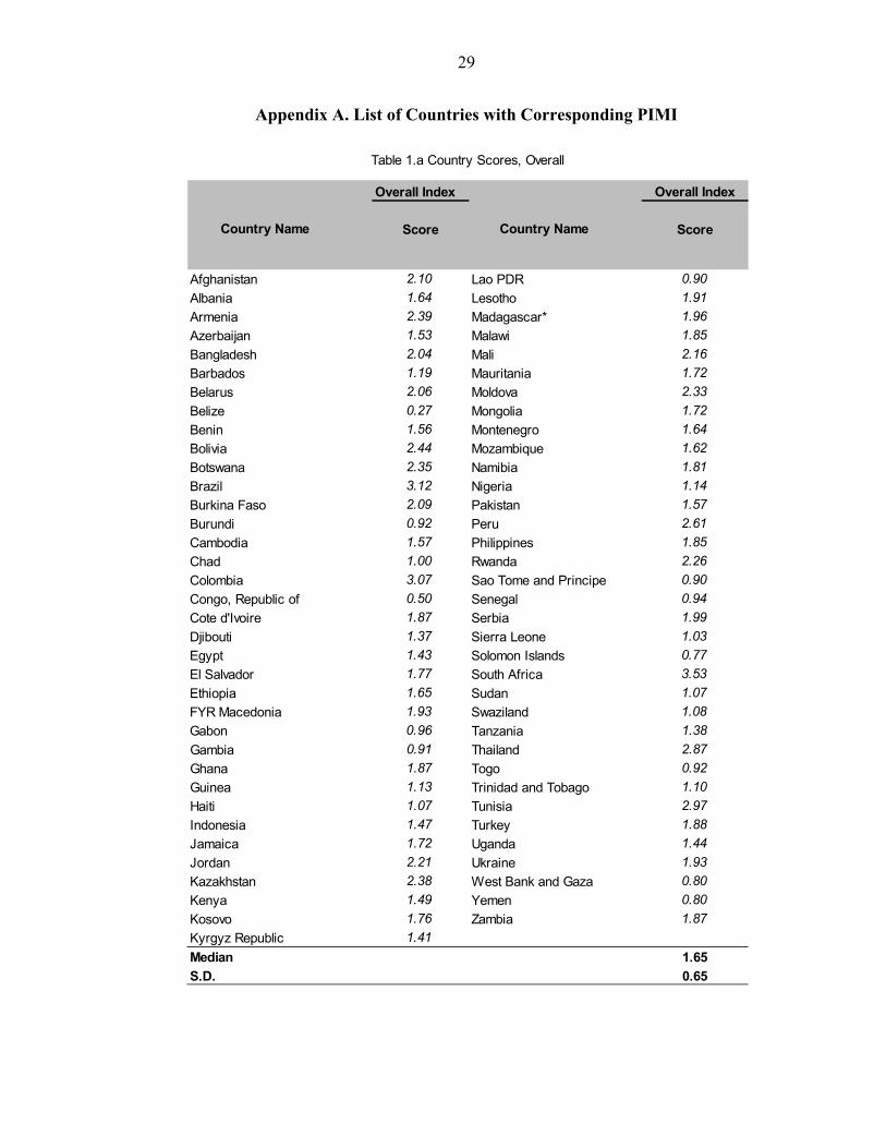
Appendix A. List of Countries with Corresponding PIMI

Overall Index

Country Name Score Country Name Score

Afghanistan 2.10 Lao PDR 0.90

Albania 1.64 Lesotho 1.91

Armenia 2.39 Madagascar* 1.96

Azerbaijan 1.53 Malawi 1.85

Bangladesh 2.04 Mali 2.16

Barbados 1.19 Mauritania 1.72

Belarus 2.06 Moldova 2.33

Belize 0.27 Mongolia 1.72

Benin 1.56 Montenegro 1.64

Bolivia 2.44 Mozambique 1.62

Botswana 2.35 Namibia 1.81

Brazil 3.12 Nigeria 1.14

Burkina Faso 2.09 Pakistan 1.57

Burundi 0.92 Peru 2.61

Cambodia 1.57 Philippines 1.85

Chad 1.00 Rwanda 2.26

Colombia 3.07 Sao Tome and Principe 0.90

Congo, Republic of 0.50 Senegal 0.94

Cote d'Ivoire 1.87 Serbia 1.99

Djibouti 1.37 Sierra Leone 1.03

Egypt 1.43 Solomon Islands 0.77

El Salvador 1.77 South Africa 3.53

Ethiopia 1.65 Sudan 1.07

FYR Macedonia 1.93 Swaziland 1.08

Gabon 0.96 Tanzania 1.38

Gambia 0.91 Thailand 2.87

Ghana 1.87 Togo 0.92

Guinea 1.13 Trinidad and Tobago 1.10

Haiti 1.07 Tunisia 2.97

Indonesia 1.47 Turkey 1.88

Jamaica 1.72 Uganda 1.44

Jordan 2.21 Ukraine 1.93

Kazakhstan 2.38 West Bank and Gaza 0.80

Kenya 1.49 Yemen 0.80

Kosovo 1.76 Zambia 1.87

Kyrgyz Republic 1.41

Median 1.65

S.D. 0.65

Overall Index

Table 1.a Country Scores, Overall

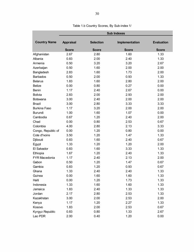
30

Country Name

Score Score Score ScoreAfghanistan 2.67 2.80 1.60 1.33

Albania 0.83 2.00 2.40 1.33

Armenia 0.50 3.20 3.20 2.67

Azerbaijan 0.50 1.60 2.00 2.00

Bangladesh 2.83 1.60 1.73 2.00

Barbados 0.50 2.00 0.93 1.33

Belarus 1.83 1.60 2.80 2.00

Belize 0.00 0.80 0.27 0.00

Benin 1.17 2.40 2.67 0.00

Bolivia 2.83 2.00 2.93 2.00

Botswana 3.00 2.40 2.00 2.00

Brazil 3.00 2.80 3.33 3.33

Burkina Faso 1.17 3.20 2.00 2.00

Burundi 1.00 1.60 1.07 0.00

Cambodia 0.67 1.20 2.40 2.00

Chad 0.00 0.80 2.53 0.67

Colombia 4.00 2.80 2.13 3.33

Congo, Republic of 0.00 1.20 0.80 0.00

Cote d'Ivoire 3.50 1.20 1.47 1.33

Djibouti 0.83 1.60 2.40 0.67

Egypt 1.33 1.20 1.20 2.00

El Salvador 0.83 1.60 3.33 1.33

Ethiopia 1.67 1.20 2.40 1.33

FYR Macedonia 1.17 2.40 2.13 2.00

Gabon 0.50 1.20 1.47 0.67

Gambia 0.83 1.20 0.93 0.67

Ghana 1.33 2.40 2.40 1.33

Guinea 0.00 1.60 1.60 1.33

Haiti 0.00 1.20 1.73 1.33

Indonesia 1.33 1.60 1.60 1.33

Jamaica 1.83 2.40 1.33 1.33

Jordan 2.17 2.80 2.53 1.33

Kazakhstan 3.00 2.00 2.53 2.00

Kenya 1.17 1.20 2.27 1.33

Kosovo 1.83 2.00 2.53 0.67

Kyrgyz Republic 0.83 0.80 1.33 2.67

Lao PDR 2.00 0.40 1.20 0.00

Appraisal Selection

Table 1.b Country Scores, By Sub-index 1/

Sub Indexes

EvaluationImplementation

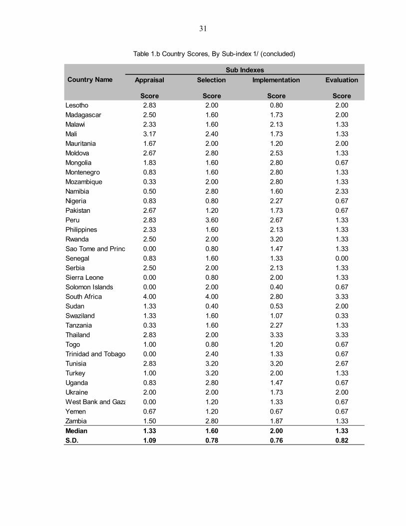
31

Country Name

Score Score Score ScoreLesotho 2.83 2.00 0.80 2.00

Madagascar 2.50 1.60 1.73 2.00

Malawi 2.33 1.60 2.13 1.33

Mali 3.17 2.40 1.73 1.33

Mauritania 1.67 2.00 1.20 2.00

Moldova 2.67 2.80 2.53 1.33

Mongolia 1.83 1.60 2.80 0.67

Montenegro 0.83 1.60 2.80 1.33

Mozambique 0.33 2.00 2.80 1.33

Namibia 0.50 2.80 1.60 2.33

Nigeria 0.83 0.80 2.27 0.67

Pakistan 2.67 1.20 1.73 0.67

Peru 2.83 3.60 2.67 1.33

Philippines 2.33 1.60 2.13 1.33

Rwanda 2.50 2.00 3.20 1.33

Sao Tome and Princ 0.00 0.80 1.47 1.33

Senegal 0.83 1.60 1.33 0.00

Serbia 2.50 2.00 2.13 1.33

Sierra Leone 0.00 0.80 2.00 1.33

Solomon Islands 0.00 2.00 0.40 0.67

South Africa 4.00 4.00 2.80 3.33

Sudan 1.33 0.40 0.53 2.00

Swaziland 1.33 1.60 1.07 0.33

Tanzania 0.33 1.60 2.27 1.33

Thailand 2.83 2.00 3.33 3.33

Togo 1.00 0.80 1.20 0.67

Trinidad and Tobago 0.00 2.40 1.33 0.67

Tunisia 2.83 3.20 3.20 2.67

Turkey 1.00 3.20 2.00 1.33

Uganda 0.83 2.80 1.47 0.67

Ukraine 2.00 2.00 1.73 2.00

West Bank and Gaza 0.00 1.20 1.33 0.67

Yemen 0.67 1.20 0.67 0.67

Zambia 1.50 2.80 1.87 1.33

Median 1.33 1.60 2.00 1.33

S.D. 1.09 0.78 0.76 0.82

Table 1.b Country Scores, By Sub-index 1/ (concluded)

Sub Indexes

Appraisal Selection Implementation Evaluation

32

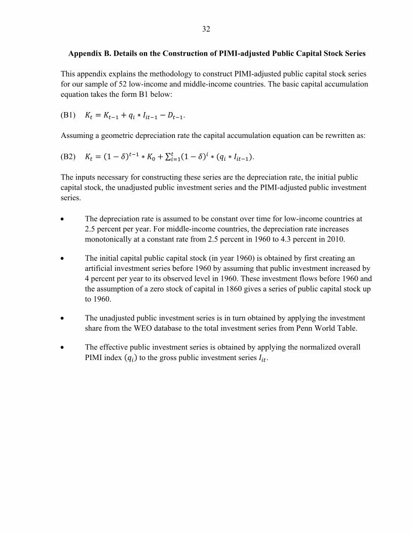
Appendix B. Details on the Construction of PIMI-adjusted Public Capital Stock Series

This appendix explains the methodology to construct PIMI-adjusted public capital stock series for our sample of 52 low-income and middle-income countries. The basic capital accumulation equation takes the form B1 below: (B1) . Assuming a geometric depreciation rate the capital accumulation equation can be rewritten as: (B2) 1 ∑ 1 . The inputs necessary for constructing these series are the depreciation rate, the initial public capital stock, the unadjusted public investment series and the PIMI-adjusted public investment series. The depreciation rate is assumed to be constant over time for low-income countries at

2.5 percent per year. For middle-income countries, the depreciation rate increases monotonically at a constant rate from 2.5 percent in 1960 to 4.3 percent in 2010.

The initial capital public capital stock (in year 1960) is obtained by first creating an artificial investment series before 1960 by assuming that public investment increased by 4 percent per year to its observed level in 1960. These investment flows before 1960 and the assumption of a zero stock of capital in 1860 gives a series of public capital stock up to 1960.

The unadjusted public investment series is in turn obtained by applying the investment share from the WEO database to the total investment series from Penn World Table.

The effective public investment series is obtained by applying the normalized overall PIMI index to the gross public investment series .

33

Appendix C. Initial Conditions and PIMI Effect on Efficiency Adjusted Capital

Assume that PIMI in 1860 same as today This case can be shown analytically.19 In continuous time, using an asterisk to indicate adjusted capital stock, and allowing for a time varying depreciation rate the motion equation of public capital is 1

which integrates to (now ignoring the i except on the q):

2 0

Meanwhile, the unadjusted capital stock K is

3 0

Comparing (C2) and (C3) gives

4 0 0

5 0 0 This says that the adjusted capital stock at any date is a country specific linear transformation of the unadjusted, where the shift part of transformation is time and country dependent. If starting value is 6 0 0

Then (C5) becomes just 7

So in this case the adjustment is just a time invariant proportional scaling down.

19 We thank Mick Keen for this derivation.

34

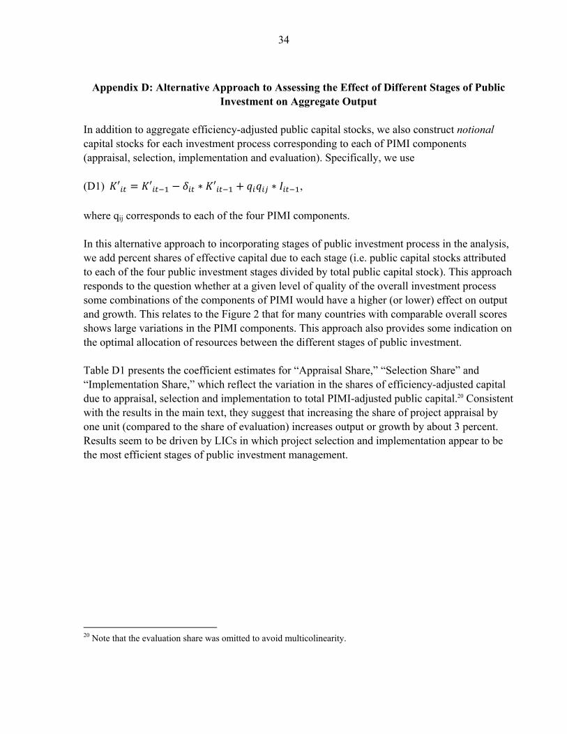
Appendix D: Alternative Approach to Assessing the Effect of Different Stages of Public

Investment on Aggregate Output

In addition to aggregate efficiency-adjusted public capital stocks, we also construct notional capital stocks for each investment process corresponding to each of PIMI components (appraisal, selection, implementation and evaluation). Specifically, we use (D1) ,

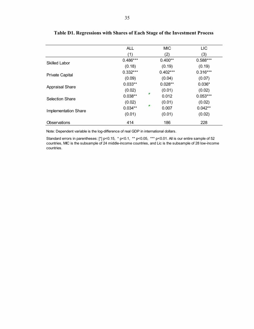
where qij corresponds to each of the four PIMI components. In this alternative approach to incorporating stages of public investment process in the analysis, we add percent shares of effective capital due to each stage (i.e. public capital stocks attributed to each of the four public investment stages divided by total public capital stock). This approach responds to the question whether at a given level of quality of the overall investment process some combinations of the components of PIMI would have a higher (or lower) effect on output and growth. This relates to the Figure 2 that for many countries with comparable overall scores shows large variations in the PIMI components. This approach also provides some indication on the optimal allocation of resources between the different stages of public investment. Table D1 presents the coefficient estimates for “Appraisal Share,” “Selection Share” and “Implementation Share,” which reflect the variation in the shares of efficiency-adjusted capital due to appraisal, selection and implementation to total PIMI-adjusted public capital.20 Consistent with the results in the main text, they suggest that increasing the share of project appraisal by one unit (compared to the share of evaluation) increases output or growth by about 3 percent. Results seem to be driven by LICs in which project selection and implementation appear to be the most efficient stages of public investment management.

20 Note that the evaluation share was omitted to avoid multicolinearity.

35

Table D1. Regressions with Shares of Each Stage of the Investment Process

ALL MIC LIC

(1) (2) (3)

0.486*** 0.400** 0.588***

(0.18) (0.19) (0.19)

0.332*** 0.402*** 0.316***

(0.09) (0.04) (0.07)

0.033** 0.028** 0.036*

(0.02) (0.01) (0.02)

0.038** 0.012 0.053***

(0.02) (0.01) (0.02)

0.034** 0.007 0.042**

(0.01) (0.01) (0.02)

Observations 414 186 228

Note: Dependent variable is the log-difference of real GDP in international dollars.

Standard errors in parentheses: [*] p<0.15, * p<0.1, ** p<0.05, *** p<0.01. All is our entire sample of 52 countries, MIC is the subsample of 24 middle-income countries, and Lic is the subsample of 28 low-income countries.

Skilled Labor

Private Capital

Appraisal Share

Selection Share

Implementation Share

36

Appendix E. Recovering the Parameters of the CES Production Function Our specification of the CES function with quality-adjusted labor, private capital and PIMI-adjusted public capital takes the following form:

(C1) 1 . H and L stand for human capital and labor, respectively. and denote private capital and PIMI-adjusted public capital, respectively. Taking logs gives:

(C2) log log log log 1 .

The first-order linearization around 0 gives: (C3) log log log 1 log 1 1 log

1 log log . This can be rewritten in the following form that can be directly estimated: (C4) log log log log log log log . The parameter is directly identifiable from the results of the regression. Other parameters of the CES function need however to be recovered. The following equations help identify each of these parameters:

1 , 1 1 ,

1 12

.

These equations can be solved in the unknown parameters of the CES function that are not directly estimated:

; 1

; 2

.

Documents

Efficiency-Adjusted Public Capital and Growth,. IMF ... · Efficiency-Adjusted Public Capital and Growth ... This paper constructs an efficiency-adjusted public capital stock series