Embed Size (px)
Citation preview
Effects of Water Based Drilling Mudson Recolonization of Sandy Soft Bottom
Communities
Ashild Setvik
MASTER THESIS IN MARINE BIOLOGY
DEPARTMENT OF BIOLOGY
FACULTY OF MATHEMATICS AND NATURAL SCIENCES
UNIVERSITY OF OSLO
June 18, 2010

2

Forord
Denne oppgaven ble utført ved Biologisk institutt i perioden 2009-2010 som en del avprosjektet “Parameterisation of the Environmental Impacts on Bottom Fauna of Water-based Drilling Fluids and Cuttings – Field and Meso-cosm Experiments” (PEIOFF-FAME),med støtte fra Norsk forskningsrad.
Jeg vil først og fremst takke mine flinke veiledere Torgeir Bakke og Hilde CecilieTrannum pa NIVA for god hjelp, konstruktiv kritikk, svar pa mine evinnelige e-poster oghjelp pa laben.
Takk til Rita som hjalp meg med alt det praktiske pa laben, takk til Hilde, Gun-hild og Marijana for hjelp til identifisering. Takk til Brage Rygg pa NIVA for hjelp tilfødegruppeanalyse og for a sjekke at artslista mi var korrekt. Takk til Ragnhild som harvært min flinke engelsklærer som fikk orden pa engelsken min. Ikke minst, takk til DagSverre, mannen min, som hjalp meg med de statistiske analysene, bade med og produseredisse og forsta, forvirre og oppklare for meg.
Takk til besteforeldre, gode naboer og spesielt kusine Anne som har vært barnevakterfor oss i en travel periode. Takk til Fredrikke som har gitt oss mer eller mindre gode mid-dager nar vi har hatt det for travelt til a lage middag. Til slutt vil jeg takke min nydeligefamilie, spesielt Astrid som er var solstrale. Gleder meg til a tilbringe mer tid med dereframover.
Universitetet i Oslo, 18. juni 2010Ashild Setvik
3

4
Abstract
This study is part of a larger research project, Parameterisation of the EnvironmentalImpacts on Bottom Fauna of Water-based Drilling Fluids and Cuttings – Field and Meso-cosm Experiments (PEIOFF-FAME). The goal was to investigate the impact of drill cut-tings when drilling with water-based drilling fluids on recolonization of a benthic ecosys-tem. Drill cuttings from oil and gas installations contain either oil-based, synthetic orwater-based muds. Today only cuttings from water-based muds are allowed to be dis-charged. Drill cuttings from water-based muds are expected to cause only minimal dam-age to the biota surrounding the installations offshore, but this statement has not beentested experimentally in the field.
My approach was a field experiment where defaunated sandy sediment treated withwater-based cuttings was deployed at the seafloor as substrate for settling benthic larvae.
Test sediment was sampled in the Oslofjord in March 2007. Drill cuttings were addedin a pattern of 0, 6 and 24 mm top layer in the boxes. Four experimental frames were de-ployed at 60 m depth on 21st of March and recaptured 6 months later on 24th of septem-ber. The data were investigated by univariate and multivariate statistical techniques.
The polychaet Ophelina acuminata showed a significant decline in abundance as afunction of layer thickness of drill cuttings, and there was an overall negative trend inrecolonization with treatment. The echuiuran Echiurus echiurus showed a weak positivetrend which was close to significant. A weak positive trend was also found for number oftaxa and for the Hurlbert’s rarefaction diversity index. There was no grouping of the boxesof test sediment as function of treatment, but there was a clear grouping as a function offrame. The test sediment had a markedly larger grain size than the drill cuttings, whilethe grain size in the fine material was similar to the drill cuttings. Analysis of the oxygenpenetration depth showed a weak negative trend as a function of added drill cuttings.
Settling communities may not be as sensitive as established communities. However,since there was a negative trend as a function of added drill cuttings it is not impossiblethat natural variation covers an effect of the drill cuttings in the field.
5

6

Contents
Preface 3
Abstract 5
1 Introduction 91.1 Characteristics of drilling muds and cuttings . . . . . . . . . . . . . . . . 9
1.1.1 Water based drilling muds (WBM ) . . . . . . . . . . . . . . . . 11
1.1.2 Oil based drilling muds (OBM) . . . . . . . . . . . . . . . . . . 12
1.1.3 Synthetic based drilling muds (SBM) . . . . . . . . . . . . . . . 13
1.2 Recolonization of benthic fauna . . . . . . . . . . . . . . . . . . . . . . 13
1.3 Settling of benthic larvae . . . . . . . . . . . . . . . . . . . . . . . . . . 15
1.4 Previous related studies . . . . . . . . . . . . . . . . . . . . . . . . . . . 17
1.5 Objective of this study . . . . . . . . . . . . . . . . . . . . . . . . . . . 17
2 Materials and Methods 192.1 Test sediment, eksperimental design and fieldwork. . . . . . . . . . . . . 19
2.2 Species identification . . . . . . . . . . . . . . . . . . . . . . . . . . . . 22
2.3 Grain size analysis and oxygen penetration . . . . . . . . . . . . . . . . . 23
2.4 Data analysis . . . . . . . . . . . . . . . . . . . . . . . . . . . . . . . . 24
3 Results 273.1 Grain size analysis and oxygen penetration . . . . . . . . . . . . . . . . . 27
3.2 Univariate analysis . . . . . . . . . . . . . . . . . . . . . . . . . . . . . 28
3.2.1 Faunal diversity . . . . . . . . . . . . . . . . . . . . . . . . . . . 29
3.2.2 Faunal Composition . . . . . . . . . . . . . . . . . . . . . . . . 29
3.3 Multivariate analysis . . . . . . . . . . . . . . . . . . . . . . . . . . . . 31
4 Discussion 394.1 Effects of drill cuttings on benthic communities . . . . . . . . . . . . . . 39
7

8 CONTENTS
4.1.1 Effects on faunal diversity . . . . . . . . . . . . . . . . . . . . . 414.1.2 Effects on faunal composition . . . . . . . . . . . . . . . . . . . 41
4.2 Effects of frame location . . . . . . . . . . . . . . . . . . . . . . . . . . 424.3 Environmental variables as explanatory factors . . . . . . . . . . . . . . 43
4.3.1 Total organic carbon (TOC) . . . . . . . . . . . . . . . . . . . . 434.3.2 Grain size . . . . . . . . . . . . . . . . . . . . . . . . . . . . . . 434.3.3 Oxygen penetration . . . . . . . . . . . . . . . . . . . . . . . . . 44
4.4 Conclusions . . . . . . . . . . . . . . . . . . . . . . . . . . . . . . . . . 444.5 Limitations . . . . . . . . . . . . . . . . . . . . . . . . . . . . . . . . . 45
Bibliography 49
References 50
A Tables 59
B Figures 73
Chapter 1
Introduction
1.1 Characteristics of drilling muds and cuttings
Drilling mud is a mixture of clay, chemicals, water or oil. There are three types of drillingmuds; water based (WBM), oil based (OBM) and synthetic based (SBM). The mud hasseveral important functions when drilling for oil. It lubricates and cools the drilling bitduring drilling and it also brings mass from the drilling to the surface. The drilling mudwill also prevent that the wall in the drilling hole collapses and it keeps the pressure inthe well under control. If the weight of the drilling muds is too low, the pressure in thewell can push oil or gas to the surface (blowout). If the weight of the drilling muds is toohigh, the mud can disappear in to the reservoir and close the pores (OLF, 2009). Otherfunctions of drilling mud are: seal permeable formations of the borehole, suspend cuttingswhen circulation is interrupted such as when adding a new piece of drillpipe, support partof the weight of the drillstring through buoyancy, and ensure the securing of important in-formation about the formation being drilled to permit its successfull evaluation (Hinwoodet al, 1994).
A type of weight material is used to apply counter-pressure in the process. Commonmaterials are barite, ilmenite, hematite and brines where barite and ilmenite are the mostcommon types. Barite (BaSO4) is a mineral consisting of barium sulphate. Barium is in-active, but may have a negative effect on biota if the concentrations become high (Olsgardand Gray, 1995). Barite is more or less polluted with Mercury and Lead. It is possibleto clean the Barite to remove the toxic substances. The other most common material isilmenite (FeTiO3). Since both ilmenite and barite are inactive they make useful tracers ofdispersion and transport of discharges related to drilling activities such as drilling mudsand cuttings (Neff, 2005; OLF, 2009). About 1000 products available for formulation of
9

10 CHAPTER 1. INTRODUCTION
drilling fluids and the total number of ingredients in most drilling fluids is in the range of8-12 (Holdway, 2002).
Drill cuttings are particles of crushed rock created by the grinding action of the drillbit as it penetrates the earth and is brought to the surface. The diameter is usually lessthan 1 cm (Neff, 2005; OLF, 2009). Drill cuttings (only water-based) are released intothe environment after separation from the mud on the platform (Davies et al, 1984).
There are no general restrictions on the release of drill cuttings from water based muds(WBM) into the environment. The reason for this policy is that bringing the drill cuttingsto shore will give higher releases in the air and demand more space for storage. Someareas are protected; no drilling fluid or drill cuttings are allowed to be released in the Bar-ents sea and Lofoten and the areas around (Klif, 2009)(Norwegian Climate and PollutionAgency). Drill cuttings from topholes can normally be released in the Barents sea, underthe condition that the release does not contain substances with unacceptable environmen-tal properties and only in areas where the potential harm on vulnerable environmentalcomponents are considered low. Klif has determined that it is important to do thoroughresearch on possible effects of future releases of cleaned cuttings with oil content less thanone weightprocent (Klif, 2009). There is a zero release policy for substances harmful tothe environment, and drill cuttings are part of this policy. Practically, this means that drillcuttings from water based muds are released, except in vulnerable ecosystems. The twoother types of cuttings are not allowed released other than under particularly demandingconditions (Klif, 2010).
The release of drill cuttings spreads different types of contaminants to the bottom ofthe sea. Around many of the installations there are high heavy metal concentrations withnegative biological effects; copper, cadmium and zinc (Olsgard and Gray, 1995). Theheavy metals in drill cuttings are likely to be distributed in the same manner as Ba (Re-naud et al, 2008). Total hydrocarbon (THC) concentrations show a clear decline overtime in the field in the surface layer of the sediment, which is probably because of dis-continuation of OBM use in 1991 (Klif, 2010; Olsgard and Gray, 1995). When it comesto fauna, monitoring programmes have been performed since the mid 1970s and annu-ally since 1985. Many of the oil fields have been sampled and the fauna examined byunivariate and multivariate methods, looking at both biological and environmental factorsthrough classifications and ordinations (Olsgard and Gray, 1995). Previous results sug-gest that the communities surveyed are partly structured by depth related factors (organiccontent, grain size), but there is some indication that disturbance makes up a much of thesecondary axis for most of the fields with installations. In multivariate analysis (MultiDimensional Scaling, MDS) of observations of benthic fauna beneath and around explo-
1.1. CHARACTERISTICS OF DRILLING MUDS AND CUTTINGS 11
ration wells (later oil platforms), stations are often grouped regardless of their distancefrom the installation, which suggests that other factors that are specific to each field aremostly responsible for structuring communities (Olsen et al, 2007). It is therefore usefulto look at results from field experiments where it is easier to rule out confounding factorsthat are specific to each field.
Discharge of solid waste (drill cuttings) from offshore drilling operations is often con-taminated by an organic phase from the mud to facilitate drilling. When sinking, mostof the cuttings will place themselves near the installation, and can stay in the environ-ment for many years (Schaanning and Bakke, 2006). Dispersion of particles from drillcuttings are greatly influenced by their particle size and the prevailing current regime.The distribution usually follows the currents, often producing an ellipsoidal distributionat the seafloor. However, it is believed that cuttings from oil-based mud drilling, fall moredirectly to the seabed compared to WBM and SBM as a result of agglomeration (Davieset al, 1984). It is therefore common to find deposits of oil based drilling muds releasedbefore 1993 when cuttings from OBM with oil content >1% was prohibited to release onthe Norwegian shelf (Schaanning and Bakke, 2006).
Since the beginning of the Norwegian oil adventure several surveys have been ex-ecuted in the field to monitor the fauna around the different installations (Olsgard andGray, 1995; Gray et al, 1999; Renaud et al, 2008). Historically, most drilling operationsin the North Sea have used WBM. However, in some drilling operations it is difficult touse WBM primarily because of hole instability caused by the swelling of water-absorbingrock. Problems of this type can be greatly alleviated by using mud suspended in an oilbase instead of water (Davies et al, 1984).
1.1.1 Water based drilling muds (WBM )
Originally, all drilling muds used in drilling operations were in an aqueous solution, butthese were later replaced by oil-based because it was preferable in drilling operations(Olsgard and Gray, 1995). Water based drilling muds (WBM) consist of fresh or salt watercontaining a weight agent (usually barite: BaSO4), clay or organic polymers, and variousinorganic salts, inert solids, and organic additives to modify the physical properties of themud so that it functions optimally (Olsgard and Gray, 1995). Ingredients list for waterbased mud can be divided into 18 categories:
Weighting materials
Viscosifiers
Thinners, dispersants
Alkalinity, pH-control addi-
tives
Bactericides
Filtrate reducers
Flocculants
Foaming agents

12 CHAPTER 1. INTRODUCTION
Lost circulation materials
Pipe-freeing agents
Calcium reducers
Corrosion inihibitors
Emulsifiers
Defoamers
Shale control inhibitors
Surface-active agents
Temperature stability agents
Lubricants
(Neff, 2005)(and references therein). Water based drilling muds also contain severalmetals, the ones of greatest concern because of their toxicity and/or abundance in drillingmuds include arsenic, nickel, chromium, barite, cadmium, copper, iron, lead, mercury andzinc (Neff, 1987; Neff et al, 2000). A typical discharge of drill cuttings from WBM willcontain between 5% and 25% drilling muds discharge after passing through the solidscontrol equipment on the platform. Drill cuttings produced during drilling with WBMmay contain a small amount of petroleum hydrocarbons. These may originate from spot-ting fluids and lubricants added to the mud, or from geological strata penetrated by thedrill (Neff, 2005). Water based drilling muds contain a appreciably amount of organicmatter, and one important ingredient is glycol. This substance is highly degradable, andwith low toxicity (Schaanning et al, 2008). Degradation may supress H2S and makethe environment highly anoxic (M Schaanning, 2010, pers. com). WBM are more finegrained (than OBM) and can be expected to lead to a wider dispersion of barite (Olsgardand Gray, 1995). Because of the quick dispersion, cuttings from WBM do not affect theenvironment in the same way as cuttings from OBM and SBM (Neff, 2005).
1.1.2 Oil based drilling muds (OBM)
Oil based drilling muds contain a refined petroleum product, usually diesel fuel, min-eral oil or a parafin mixture (Neff, 2005). In the beginning, OBMs contained diesel oil.This was later exchanged with mineral oil, mainly because of the work conditions for theworkers at the oil platforms. Mineral oil did not significantly improve the environmentalconditions (Bakke et al, 1986). Drill cuttings from OBM with an oil content of maximum6 % on Norwegian sector was before 1st of January 1993 permitted to release duringdrilling operations. After 1st of January 1993 intentional discharge of oil-contaminatedcuttings was prohibited on the Norwegian continental shelf (Gray et al, 1999). Underdrilling conditions where the technical properties of OBM are needed for safety or op-erational reasons, OBM may be used after approval of the Norwegian authorities (Klif,2009), for instance when drilling in shale formations (Neff, 2005). The cuttings fromOBM that are allowed to be released must have a oil content below 1 % (Berge, 1993).If OBM cuttings are used it will pass through treatment facilities such as shale shakers,desanders, desilters and mud cleaners to separate the cuttings from the mud and maintain

1.2. RECOLONIZATION OF BENTHIC FAUNA 13
the desired mud formulation (Davies et al, 1984). With the discharges of OBM, apprecia-bly amounts of hydrocarbons and heavy metals were released into the environment. Highoil concentrations were found close to some of the major OBM operations (both dieseland alternative mud users), typically between 1000 to 10000 times background within 250m of the platform. The concentrations fall steeply, generally reaching background levelswithin 3000 m. The extent of biological effects from oil-based mud cuttings is greaterthan the extent from water-based mud cuttings. Beyond the area of physical smother-ing, the effects of oil-based mud cuttings may be because of organic enrichment of thesediment and/or the toxicity of certain fractions of the oils used, such as aromatic hydro-carbons. It is not possible from the present available results to distinguish between theecological effects of diesel mud and alternative base mud (Davies et al, 1984).
The amount of drill cuttings released from OBM between 1983 and 1992 are estimatedto be around 300,000 tonnes distributed on average 92 wells per year. Heights of thecuttings piles varied between <2m to 15m, with the most cuttings piles being less than2m or 7-15m tall (Cripps et al, 1998).
1.1.3 Synthetic based drilling muds (SBM)
To replace OBM, synthetic based muds (SBM) were developed. They are contaminatedwith organic fluids such as ethers, esters and olefins that were meant to replace the mineraloil in OBM (Schaanning and Bakke, 2006). Common substances in SBMs are olefins, es-ters, ethers, polyalphaolefins, glycols, glycerins and glucosides. These chemicals areintended to make the muds having the advantages of oil muds but with the handlingand disposal characteristics of water muds (Caenn and Chillingar, 1996). In Norway,synthetic-based drilling muds were used in the period around 1990-2000. Around 2000 itwas forbidden to use SBM with organic content > 1 % because of the effects on the en-vironment. Benthic effects of SBM were recorded up to 500 m from the platform (Jensenet al, 1999). SBM contains little substances harmful to the environment, but the highorganic content leads in many cases to anoxia and bad conditions for the benthic fauna(Neff et al, 2000).
1.2 Recolonization of benthic fauna
One can assume that studies on recolonisation of contaminated sediments provide relevantinformation about species tolerance of contaminants (Trannum et al, 2004). Recoloniza-tion and succession in soft sediments have been studied extensively (see (Gray, 1981;

14 CHAPTER 1. INTRODUCTION
Probert, 1984; Thrush, 1991)). Dominance in the early phase of recolonization appears tobe determined by the availability of benthic species/larvae at the time the habitat was madeavailable (Grassle and Grassle, 1974; Pearson and Rosenberg, 1978). Dense aggregationsof polychaete tubes are often considered to stabilize sediments by altering the character-istics of near-bed waterflow and have been shown to be particulary important in affectingearly stages of succession (Sanders et al, 1962; Fager, 1964; Gallagher et al, 1983; Levin,1985). Timing of initial colonization seems to be an important factor that controls de-velopment of experimental populations, since postlarvae and juveniles are available aspotential colonizers change depending on the season of the year (Diaz-Castaneda et al,1993). Initial recolonization after defaunation in marine soft bottom sediment is pre-dominant by opportunistic species with r-selected life-history traits, such as capitellid andspionid polychaetes. Species termed opportunists have evolved life-history characteristicssuch as rapid dispersal and high reproductive rates that allow them to locate and colonizedisturbed patches rapidly so that these species occur early in succession. Other specieswhich are better resource competitors invade later and displace the opportunists only tobe displaced by succeeding colonists themselves (Thistle, 1981).
Certain qualities characterize species that are typical in the initial phase of recolo-nization; (1) opportunistic (many reproductions per year, high recruitment, rapid devel-opment, early colonizers, high death rate), (2) small, (3) sedentary, (4) deposit feeders(mostly surface feeders) and (5) brood protection (lecithotrophic larvae). Average lifespan, generation time and population growth rate set the pace of population processes(Zajac et al, 1998)
Biological interactions become more important in the later successional stages, andaccumulation of toxic metabolites may also become a limiting factor. The abundant initialcolonizers may often be replaced at a later succesional stage (Grassle and Grassle, 1974;Connel and Slatyer, 1977; McCall, 1977).
Some biotic processes influence the process of recolonization. Facilitation comprisesinteractions in which one group of organisms enhances the establishment of another. In-hibition results in groups of organisms preventing or significantly reducing the establish-ment of another group. This may occur via competition for resources such as food and/orspace. Predation can also be added to the list (Zajac et al, 1998).
Hydrodynamics also affect the distribution of food resources which may have a criticalrole in shaping successional dynamics in soft-sediment habitats (Thistle, 1981).
The mode of recolonization (e.g., contribution of larval vs. post-larval dispersal) ofdisturbed habitats appears to be scale dependent (Gunther, 1992). Thus, understandinghow the spatial scale of recolonization influences this mode is important in developing
1.3. SETTLING OF BENTHIC LARVAE 15
realistic models of patch and community dynamics (Smith and Brumsickle, 1989; Thrushet al, 1996). As the spatial scale of disturbances increases, the duration of successiverecovery should increase (Zajac et al, 1998).
The experimental environment facilitates the survival of young organisms on defau-nated test plots. There is no competition and lower rates of predation when compared withthe natural environment, and there is a high content of organic matter which favours thesettlement of deposit feeders (Zajac et al, 1998). In recolonization experiments with de-faunated sediments the abundance will increase to a certain point, reach peak after sometime, followed by a decline in number of individuals. The number of species shows asimilar trend (Lu and Wu, 2000).
1.3 Settling of benthic larvae
“Settlement“ is the process by which planktonic larva moves toward the substratum, ex-plores, attaches to the substratum, and begins its benthic life (Quian, 1999). Settlingof benthic invertebrate larvae is an important part of the recolonization process. Distur-bances such as the release of drill cuttings can possibly be a disturbance that can influencethis process. The larval and juvenile stages are considered the most vulnerable stages ofmarine invertebrates, and might be particularly vulnerable to pollution (Woodin, 1976;Jablonski and Lutz, 1983), in this context from drill cuttings. The larvae of opportunisticspecies normally have little or no selectivity in their substratum requirements (Pearsonand Rosenberg, 1978).
Larval development can be split into to groups; planktonic and benthonic, and somespecies brood larvae to different extents and release them into the plankton for variousperiods of time (Olive and Clark, 1978). We have a good understanding of the settlingof benthic invertebrate larvae, but the planktonic phase of benthic larval organisms isless known (Eckman, 1996). Life cycles of most benthic marine invertebrates speciesinclude microscopic, free-living dispersive stages that may be feeding (planktotrophic) ornon-feeding (lecithotrophic) (Pechenik, 1999). Some controlled experiments have beencarried through to learn more about the settlement stage in the life cycle of benthic organ-isms. Species of marine invertebrates with a planktonic larval stage differentiates into aplanktotrophic trochopore and then a metatrochophore (Marsden et al, 1990). The plank-tonic phase of invertebrate larvae may last from minutes to months. (Pawlik, 1992). Justbefore metamorphosis and settlement, the larvae become demersal, moving slowly alongthe bottom. Some species show a clear preference for certain habitats (Marsden et al,1990).

16 CHAPTER 1. INTRODUCTION
It is possible for post-larvae to move on mudflats, although it is usually assumedthat postlarvae are only capable of moving short distances (Thrush et al, 1996; Smithand Brumsickle, 1989). The process for polychaet larvae settlement is a dynamic eventbecause the larvae can leave one site and select another for settlement (Quian, 1999).However, sooner or later the larvae has to settle because it will eventually metamor-phose. Interaction between the larvae and the substratum will therefore determine thesite of larval settlement on small spatial scales and may determine postsettlement mor-tality of larvae (Quian, 1999) (and references therein). This interaction can be affectedby biological, physical or chemical factors, such as community structures, presence orabsence of natural inducers released by conspecific individuals, biofilms, prey species,or sympatric species (Quian, 1999) (and references therein). One author suggests thatchemical cues from adults or adult sites in the form of dissolved material may induceorientation behaviour by presettlement larvae (Burke, 1986). Several compounds can in-duce settlement in marine larval polychaetes; (1) juvenile hormones, (2) free fatty acids,(3) polysaccharides, (4) proteins and small peptides, (5) amino acids, (6) inorganic ionsand (7) neurotransmitters (Quian, 1999) (and references therein). Water currents and flowdynamics may determine both vertical and horizontal distribution of larvae in a water col-umn. Swimming and adhesive behaviour is of some importance if the larvae are movednear the substratum by currents (Quian, 1999). Video observations of competent larvaehave shown that the animal swim primarily on the horizontal plane, about a centimeterabove the bed, frequently testing the substratum by swimming down to the bottom andswimming away in the absence of an appropriate cue. This is the first demonstration (tothe authors knowledge) that infaunal species can actively select a preferred habitat in arealistic, turbulent flow (Butman et al, 1988).
The following factors has been shown to inhibit the successfull settlement of somebenthic larvae; oxygen depletion (Arntz, 1977), sediment instability (Rhoads and Young,1970; Rhoads et al, 1977) and pollution (Bellan et al, 1972). Drill cuttings have propertiesthat can influence the settling of larvae and possibly cause such conditions to develop inbenthic communities.
After settling, postsettlement mortality and emigration can determine the successof the larvae that initiate metamorphosis (Watzin, 1983; Luckenbach, 1984; Eyster andPechenik, 1987)
1.4. PREVIOUS RELATED STUDIES 17
1.4 Previous related studies
Effect of Barite (BaSO4) on development of estuarine communities has been studied in alaboratory experiment. The authors found that large quantities of this compound might ad-versely affect the colonizing of benthic animals (Tagatz and Tobia, 1978). An experimentwith different level of exposure from drill cuttings on larva was executed to observe theeffect on larval development, where the largest levels of drill cuttings added showed lowerdensities and fewer species (Menzie, 1984). Field experiments on benthic recolonizationand chemical changes in response to various types and amounts of cuttings, both waterbased and oil based have been done in Raunefjorden, western Norway. The fauna wasgreatly affected by the OBM drill cuttings, although effects on WBM drill cuttings werenot present (Bakke et al, 1986). The effects on defaunated sediment contaminated withcrude oil was studied in two Norwegian fjords with unequal eutrophication status. Theunpolluted Raunefjord in Western Norway was affected by the oil with lower densities,caused by toxic response to the oil directly leading to increased mortality (Berge, 1990)In an experiment with treated drill cuttings little effects were observed on recolonizationof benthic communities, but severe effects on oil-based cuttings with high oil content(15-20%) were observed (Berge, 1993). Assemblages of recruiting soft-sediments con-taminated by petroleum hydrocarbon were significantly affected in a field experiment atCasey Station, Antarctica (Stark et al, 2003). Effects of WBM cuttings were observed in amesocosm experiment in established soft-bottom communities (Trannum et al, 2009)(alsoin PEIOFF-FAME). A study of effects of WBM cuttings in the field with its current com-position is lacking.
1.5 Objective of this study
This study is part of a larger research project, Parameterisation of the EnvironmentalImpacts on Bottom Fauna of Water-based Drilling Fluids and Cuttings – Field and Meso-cosm Experiments (PEIOFF-FAME), and some results or measurements from other partsof the experiment have therefore been included wherever necessary. The main objectiveof PEIOFF-FAME are to provide quantitative results on effects of WBM drill cuttingsdischarges on bottom fauna through new mesocosm- and field experiments, together withexisting results and literature observations and quantitative observations on the most im-portant factors relevant for a realistic parameterisation of the ERMS- model (Environ-mental Risk Management System) (Olsgard et al, 2005).
The main objectives of this study are (through a field experiment):

18 CHAPTER 1. INTRODUCTION
• to assess the relationship between the dose of WBM cuttings and the effects onthe benthic ecosystem; faunal composition, diversity, individual species, groups ofspecies or ecological groups.
• to investigate if change in environmental variables such as oxygen penetration depth,grain size and total organic carbon can explain possible negative effects of the drillcuttings (Olsgard et al, 2005).
This part of the study was done on coarse sediment (sand), another was done on finesediment (clay). A third part had coarse sediment (sand) as “treatment” on fine sedimentsand fine sediment (clay) as “treatment” on coarse sediment as controls, on order to lookfor particularly for the effect of grain size. In this experiment the boxes without treatment(only sand) serve as controls and will be treated as controls. The null hypothesis testedis that there is no decline in abundance or diversity as a function of the added WBM drillcuttings thickness layer in the experiment. The results from the experiments will in itselfbe highly relevant for the future management of drilling activities in temperate, borealand arctic waters (Olsgard et al, 2005).

Chapter 2
Materials and Methods
2.1 Test sediment, eksperimental design and fieldwork.
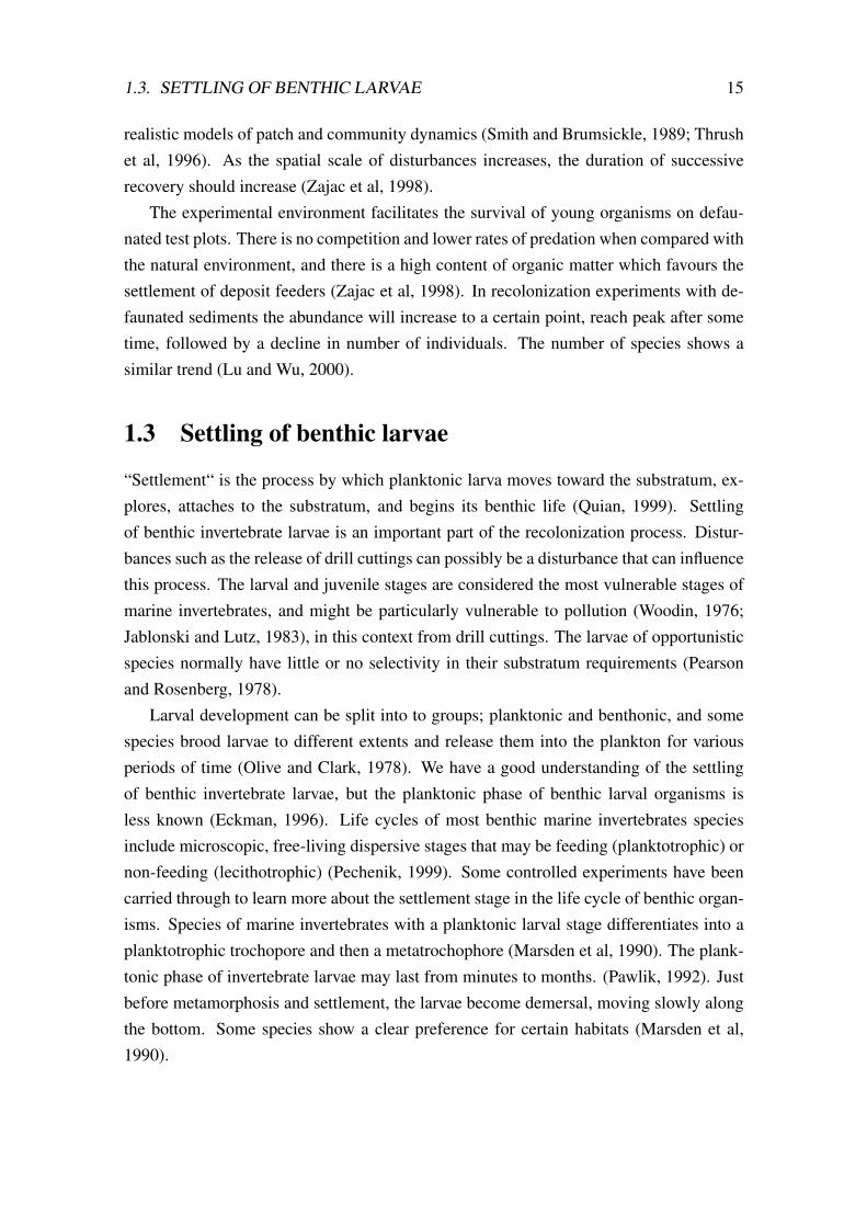
Sediment samples were collected at two locations at 116 and 96 m depth in the outerpart of inner Oslofjord (59,643◦N/10,629◦E, /59,652◦N/ 10,6213◦E) representatives ofa fine and coarse sediment with a 0.1 m2 Van veen grab on the 3rd and 5th of March2007 (figure 2.1). After the collection, the sediment was stored in 120-L PVC boxes fora maximum of 3 days at 8-10◦C. All sediments were mixed separately in batches of 30L in a cement mixer for 1 hour each. After mixing, a 10-cm-thick layer was filled into0.1-m2 propene plastic boxes (29 x 32 x 13cm) and frozen at -20◦C for at least 5 days foradditional defaunation of the sediments and to avoid loss of sediment during deployment.The drill cuttings used in this experiment is water based, with ilmenite as weight materialand contains glycol. These cuttings were used in the Barents sea before disposed on shoreon a disposal site.
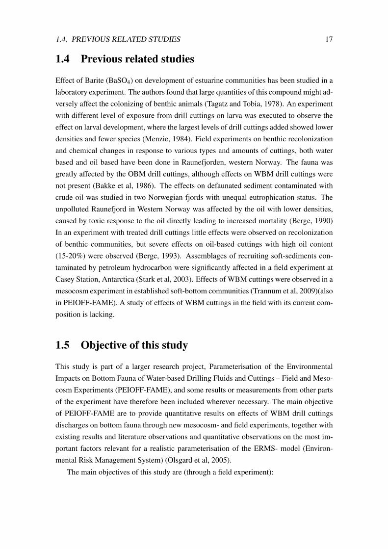
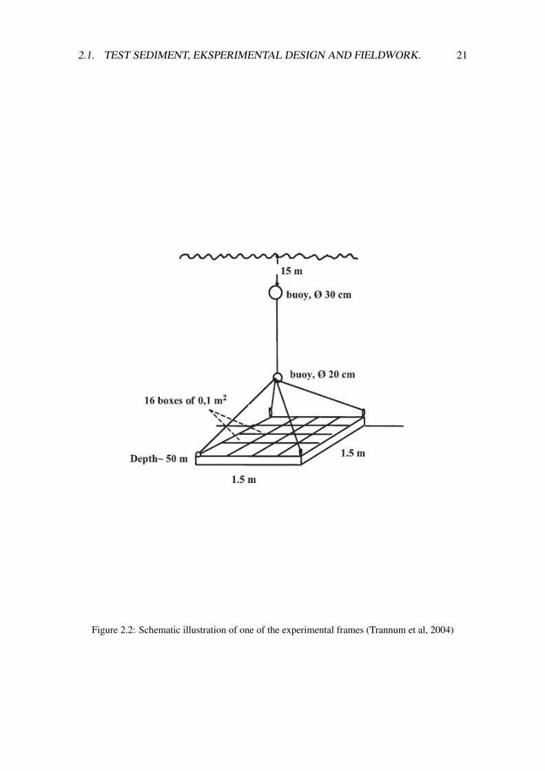
A total of 64 boxes with sediment, with or without cuttings were placed into fourseparate 1.5 x 1.5 m2 aluminium frames (figure 2.2), with 16 boxes in each frame. Theexperiment started on the 21st of March 2007 when the frames were deployed at 60 mdepth at an unpolluted location in the Oslofjord just outside Norwegian Institute of WaterResearch’s (NIVA) research station, Solbergstrand (figure 2.1). The four frames wereplaced at two different sites (in the same area as the test sediment sampling) at each sideof the fjord to avoid pseudoreplication. Frame A and B and C and D were placed at thesame location. The experimental frames were positioned about 20 cm above the seabed.
The PVC-boxes contained either sandy silt or clay. The drill cuttings were added in a6 or 24 mm top layer (table 2.1). Sandy silt and clay were also added in 6 or 24 mm toplayer and the rest were controls. The marked boxes (table 2.1) are the samples included
19
20 CHAPTER 2. MATERIALS AND METHODS
Oslo
Drøbak
Figure 2.1: Map of the Oslofjord; the red circle marks the approximate area for the experimentand the ambient grab samples. Modified after Finn Bjorklid.
Table 2.1: Setup for the frames in the experiment. All the frames had the same configuration.(S-sand,C-drill cuttings, F-fine, 6mm and 24mm layer of drill cuttings). The frames marked with(*) are the types of treatments in this master thesis.
F S(*) FF FF24FS6 FS24 FC6 FC24SF6 SF24 SS6 SS24SC6(*) SC24(*) F S(*)
in this master thesis from three of the four initial frames. In total there were initially 6control boxes (either with sand or fine material), 3 boxes with a 6mm layer of treatment(either cuttings, clay or sand) and 3 boxes with a 24mm layer of treatment. All the boxeswere placed at random in each frame. Aluminium bars screwed to the handles of eachframe held the boxes in position in the frames.
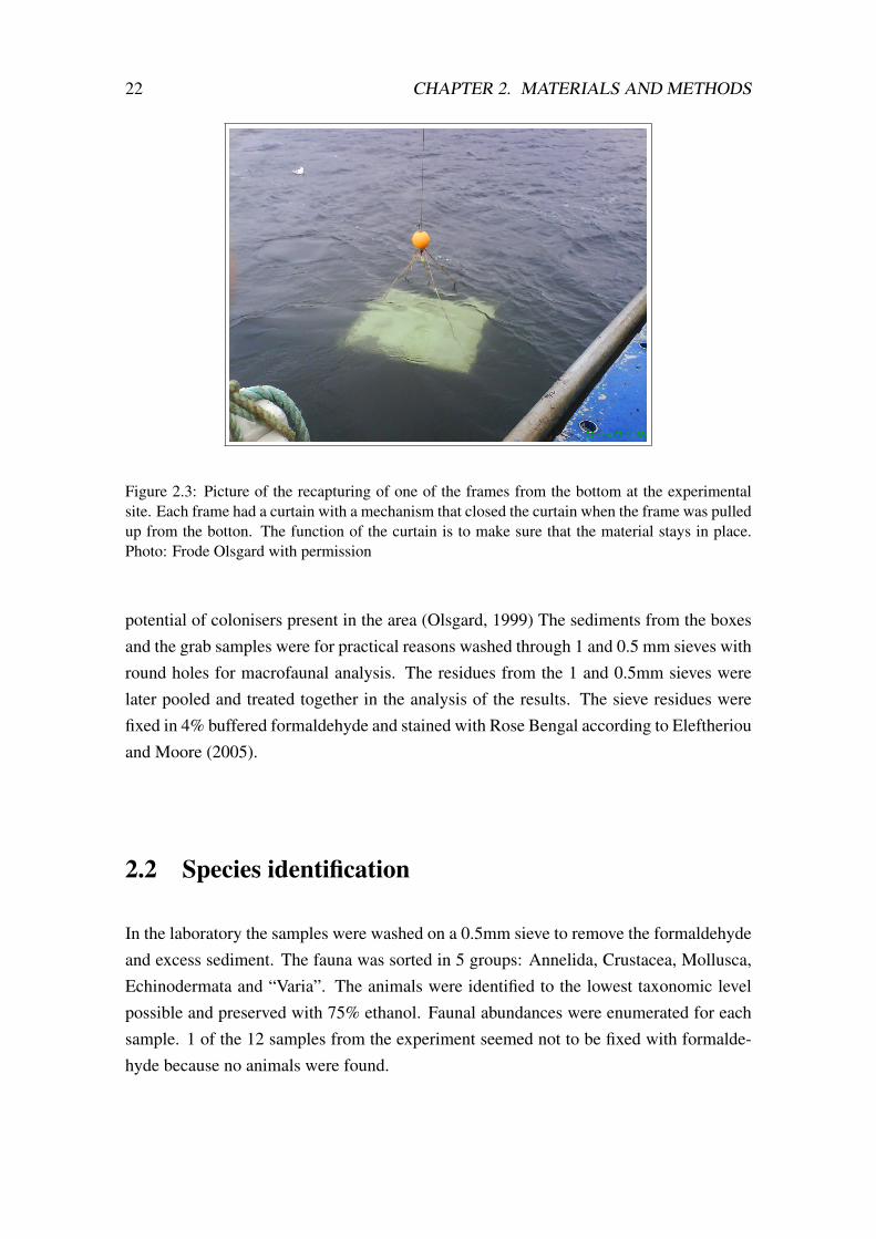
After 6 months, on the 24th of September, each underwater buoy was recaptured (fig-ure 2.3) and (figure 2.4). When the frames were brought up frame C came up in a tiltedposition so that the content did not stay in place and this frame had to be excluded from theexperiment. Two ambient (Southern and Northern) grab samples taken from the adjacentseabed are also included in the material to enable faunal comparisons with the experi-mental material. Ambient samples are collected to give a picture of the fauna and of the
2.1. TEST SEDIMENT, EKSPERIMENTAL DESIGN AND FIELDWORK. 21
Figure 2.2: Schematic illustration of one of the experimental frames (Trannum et al, 2004)
22 CHAPTER 2. MATERIALS AND METHODS
Figure 2.3: Picture of the recapturing of one of the frames from the bottom at the experimentalsite. Each frame had a curtain with a mechanism that closed the curtain when the frame was pulledup from the botton. The function of the curtain is to make sure that the material stays in place.Photo: Frode Olsgard with permission
potential of colonisers present in the area (Olsgard, 1999) The sediments from the boxesand the grab samples were for practical reasons washed through 1 and 0.5 mm sieves withround holes for macrofaunal analysis. The residues from the 1 and 0.5mm sieves werelater pooled and treated together in the analysis of the results. The sieve residues werefixed in 4% buffered formaldehyde and stained with Rose Bengal according to Eleftheriouand Moore (2005).
2.2 Species identification
In the laboratory the samples were washed on a 0.5mm sieve to remove the formaldehydeand excess sediment. The fauna was sorted in 5 groups: Annelida, Crustacea, Mollusca,Echinodermata and “Varia”. The animals were identified to the lowest taxonomic levelpossible and preserved with 75% ethanol. Faunal abundances were enumerated for eachsample. 1 of the 12 samples from the experiment seemed not to be fixed with formalde-hyde because no animals were found.
2.3. GRAIN SIZE ANALYSIS AND OXYGEN PENETRATION 23
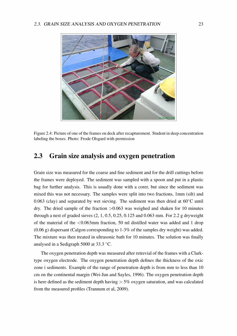
Figure 2.4: Picture of one of the frames on deck after recapturement. Student in deep concentrationlabeling the boxes. Photo: Frode Olsgard with permission
2.3 Grain size analysis and oxygen penetration
Grain size was measured for the coarse and fine sediment and for the drill cuttings beforethe frames were deployed. The sediment was sampled with a spoon and put in a plasticbag for further analysis. This is usually done with a corer, but since the sediment wasmixed this was not necessary. The samples were split into two fractions, 1mm (silt) and0.063 (clay) and separated by wet sieving. The sediment was then dried at 60◦C untildry. The dried sample of the fraction >0.063 was weighed and shaken for 10 minutesthrough a nest of graded sieves (2, 1, 0.5, 0.25, 0.125 and 0.063 mm. For 2.2 g dryweightof the material of the <0.063mm fraction, 50 ml distilled water was added and 1 drop(0.06 g) dispersant (Calgon corresponding to 1-3% of the samples dry weight) was added.The mixture was then treated in ultrasonic bath for 10 minutes. The solution was finallyanalysed in a Sedigraph 5000 at 33.3 ◦C.
The oxygen penetration depth was measured after retrevial of the frames with a Clark-type oxygen electrode. The oxygen penetration depth defines the thickness of the oxiczone i sediments. Example of the range of penetration depth is from mm to less than 10cm on the continental margin (Wei-Jun and Sayles, 1996). The oxygen penetration depthis here defined as the sediment depth having > 5% oxygen saturation, and was calculatedfrom the measured profiles (Trannum et al, 2009).

24 CHAPTER 2. MATERIALS AND METHODS
2.4 Data analysis
The faunal observations were analysed by univariate and multivariate techniques. Foreach sample (ambient grab samples and experimental samples), univarite measures in-cluded total number of individuals (N) (abundance) and total number of taxa (S) (rich-ness).
Several diversity indices were calculated. It is common to use several measures ofdiversity in the same investigation. The different ways of calculating diversity interpretthe fauna composition in different ways (Olsgard, 1995).
Shannon’s diversity index (exp H’) is given by
H ′ =−∑i
pi log(pi)
where pi is the proportion of the total count (or biomass etc) arising from the ith species(Clarke and Warwick, 2001), (Shannon and Weaver, 1963). The Shannon’s index is sen-sitive for rare species (Olsgard, 1995).
Simpson’s diversity (1-Lambda) (Simpson, 1949) has a number of forms
λ = ∑ p2i
1−λ = 1− (∑ p2i )
λ′ = ∑
i
Ni(Ni−1)N(N−1)
1−λ′ = 1−∑
i
Ni(Ni−1)N(N−1)
where Ni is the number of individuals of species i and λ is the probability that any twoindividuals from the sample, chosen at random, are from the same species (λ is always <
1) (Clarke and Warwick, 2001). Simpson’s diversity is a dominance index, in the sensethat its largest values correspond to assemblages whose total abundance is dominated byone, or a very few of the species present (Olsgard, 1995).
Pielou’s evenness index (J’) (Pielou, 1966) is given by
J′ = H ′/H ′max = H ′/logS

2.4. DATA ANALYSIS 25
where S is the number of species and H ′max is the maximum possible value of Shannondiversity, i.e. that which would be achieved if all species were equally abundant (namely,logS). (Clarke and Warwick, 2001). Pielou’s evenness index measures how even theindividuals are distributed between the species (Olsgard, 1995).
Hurlbert’s rarefaction (Sanders, 1968; Hurlbert, 1971) is given by
ESn =S
∑i=1
[1− (N−Ni)!(N−n)!(N−Ni−n)!N!
.
The method can be used to project back from the counts of total species (S) and individu-als (N), how many species (ESn) would have been ’expected’ if we had observed a smallernumber (n) of individuals (Clarke and Warwick, 2001). Hurlbert’s rarefaction is a graph-ical method for describing diversity. According to Klif (earlier SFT) guide for classifi-cation of environmental state the community (here: the box) is considered unaffected, inequilibrium and the state is classified as “good” when the ES100-value is over 18.5, whilelower values can indicate influence from pollution or some kind of disturbance (Olsgard,1995). Minitab version 15 was used to make the box plots of the diversity indices.
Regression analysis were carried out for abundance of the ten most abundant speciesfrom the experimental boxes, feeding groups, total abundance, total number of species anddiversity indices against the layer thickness of drill cuttings with the statistical programR. The faunal counts were log-transformed in order to attain equal spread.
Because it was desirable to see if the drill cuttings would affect the function of eco-logical groups of animals, the fauna was divided into the following feeding groups; (1)suspension/filter feeders, (2) surface deposit feeders, (3) subsurface deposit feeders, (4)carnivore/omnivore, (5) scavengers, (6) scrapers/grazers, (7) dissolved matter/symbionts,(8) parasites/commensals, (9) large detritus/sandlickers (see appendix for table with list offeeding mode of each species, table A.5 and table A.3 for the compiled list). The speciesgot a score for the different feeding modes; 0, 1, 2, or 3 depending on how much thespecies is one or another of the categories. If a species fit equally well into two groupsit was assigned to both groups. The traits for the feeding groups were acquired from theNIVA-database.
Multivariate analysis were carried out with nonparametric methods in the PRIMER-package (Plymouth Routines In Multivariate Ecological Research) (Clarke, 1993; Clarkeand Warwick, 2001). To analyse for similarities in community structure Multi Dimen-
26 CHAPTER 2. MATERIALS AND METHODS
sional Scaling (MDS) based on Bray-Curtis similaritiy measure was executed given by
S jk =∑
Si=1 |Xi j−Xik|
∑Si=1(Xi j−Xik)
where Xi j and Xik are the numbers of individuals of the species i at station j (Olsgard,1995). Similarities were calculated based on the fourth root counts. The purpose of theMDS is to construct a “map” or configuration of the samples, in a specified number ofdimensions (Clarke and Warwick, 2001). Cluster analysis was carried out and aim to find“natural groupings” of samples such that samples within a group are more similar to eachother, than samples in different groups. It is possible to test for significance in the MDS-ordination, the ANOSIM procedure in the PRIMER-package. Since there were only threereplicates this was not considered useful.
Chapter 3
Results
The raw data (environmental variable measurements and species abundances) are pro-vided in the appendix A.
3.1 Grain size analysis and oxygen penetration
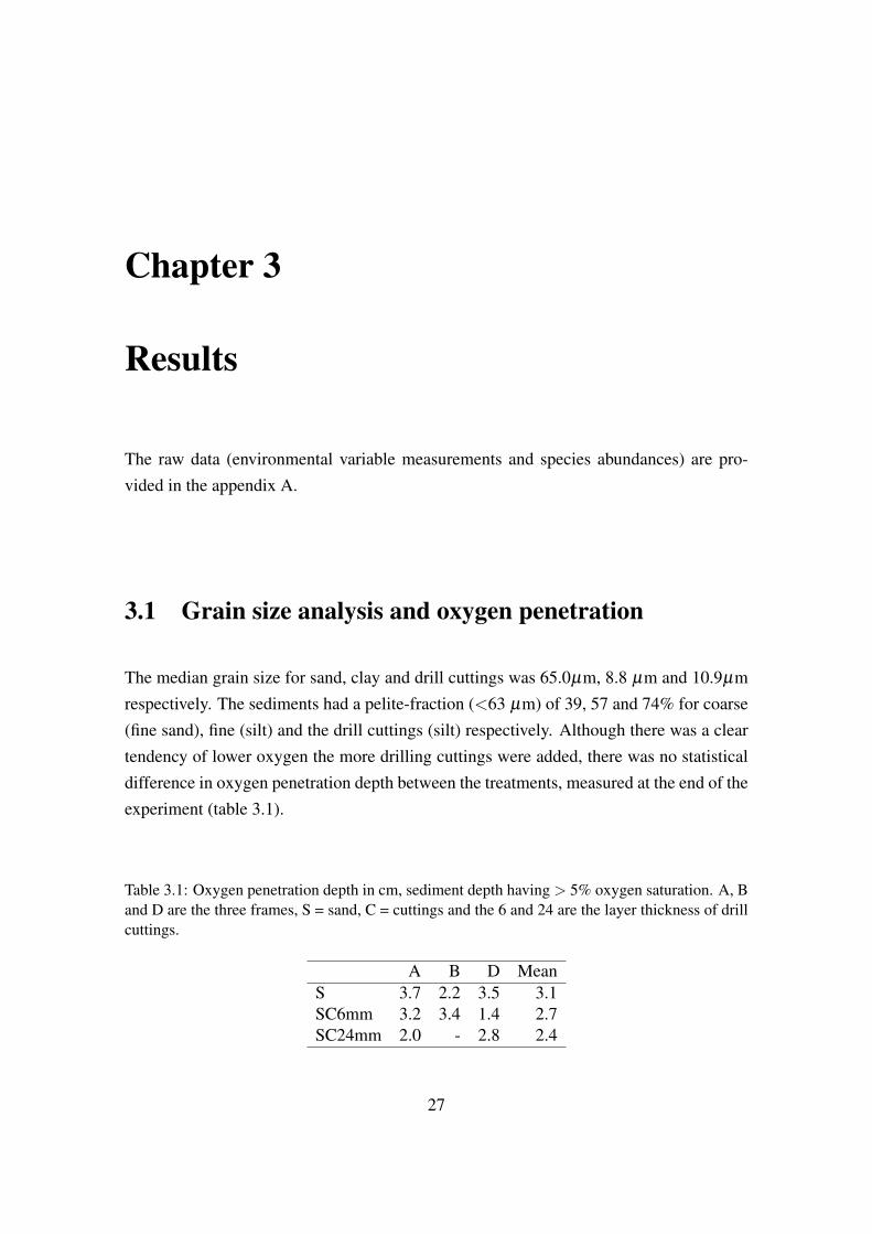
The median grain size for sand, clay and drill cuttings was 65.0µm, 8.8 µm and 10.9µmrespectively. The sediments had a pelite-fraction (<63 µm) of 39, 57 and 74% for coarse(fine sand), fine (silt) and the drill cuttings (silt) respectively. Although there was a cleartendency of lower oxygen the more drilling cuttings were added, there was no statisticaldifference in oxygen penetration depth between the treatments, measured at the end of theexperiment (table 3.1).
Table 3.1: Oxygen penetration depth in cm, sediment depth having > 5% oxygen saturation. A, Band D are the three frames, S = sand, C = cuttings and the 6 and 24 are the layer thickness of drillcuttings.
A B D MeanS 3.7 2.2 3.5 3.1SC6mm 3.2 3.4 1.4 2.7SC24mm 2.0 - 2.8 2.4
27

28 CHAPTER 3. RESULTS
3.2 Univariate analysis
A total number of 3574 animals belonging to a total of 130 species were counted in the11 boxes and the two ambient grab samples. Around 2/3 of the taxa (84 out of 130) wereidentified to the species level. Annelida (Polychaeta) was by far the dominant group,comprising 88% of the individuals and 51 % of the taxa. Crustaceans, molluscs andechinoderms made up the remainder of the samples, in addition the group “Varia” whichinluded the phyla Cnidaria, Echiura, Sipunculida, Nemertinea and Nematoda (table 3.2).
There was a slight increase in the average number of individuals in each of the treat-ments. There were on average 345 individuals in the controls, while the numbers for24mm mud and 6mm mud was 280 and 246, respectively (table 3.3). Maximum and min-imum number of individuals for each treatment are also found in table 3.3. The 6mmtreatment had 19% less animals than the controls and the 24mm treatment had 29% lessanimals than the controls on average and the 24mm treatments had 12% less animals thanthe controls. The average number of taxa in the three treatments was about equal (table3.3), but the average number of species in the ambient samples was lower.
For many of the species and feeding groups there is a negative trend as a function of thelayer thickness, but this trend is not statistically significant (figure 3.2 and 3.3). However,there are exceptions. Ophelina acuminata (p = 0.009) (figure 3.2) shows a significantdecline for the number of individuals as a function of the layer thickness of added drillingcuttings. Echiurus echiurus shows a positive trend (p = 0.09) for number of individuals asthe layer thickness of drill cuttings increased that is close to significant (figure 3.2). Lin-ear regression on the feeding groups (carnivore/omnivore, suspension feeders, subsurfacedeposit feeder, surface deposit feeders and suspension/subsurface deposit feeders) doesnot show significant p-values (figure 3.3).
Table 3.2: The total number of individuals and taxa within each phylum in all the samples (in theambient samples and the experimental boxes), and the percentage of individuals and taxa that eachphylum made up of the total abundance and species richness. Both abundance and number of taxaare absolute values.
Annelida Crustacea Mollusca Echinodermata VariaTotalt no. of individuals 3160 75 98 39 204Total no. of taxa 66 31 19 6 8% of the individuals 88.37 2.1 2.74 1.09 5.7% of the taxa 50.8 23.7 14.6 4.6 6.2

3.2. UNIVARIATE ANALYSIS 29
Table 3.3: Average abundance and average number of taxa per box in the different treatments.Averages are used to enable comparisons between the treatments.
Abundance (N) Controls 6mm 24mm AmbientMax 570 453 276 149
Average 345 280 246 135.5Min 248 186 193 122
Taxa (S) Controls 6mm 24mm AmbientMax 35 44 45 25
Average 33.6 33.7 36.3 24.5Min 30 26 29 24
3.2.1 Faunal diversity
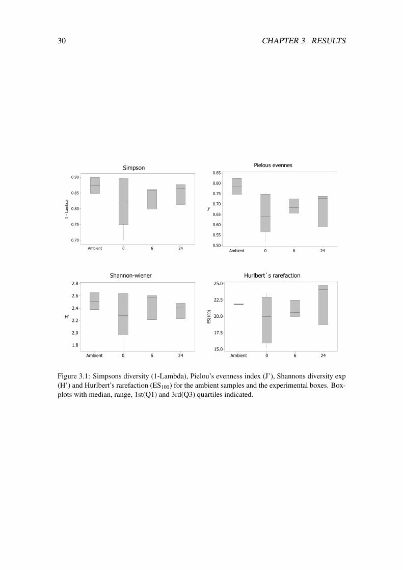
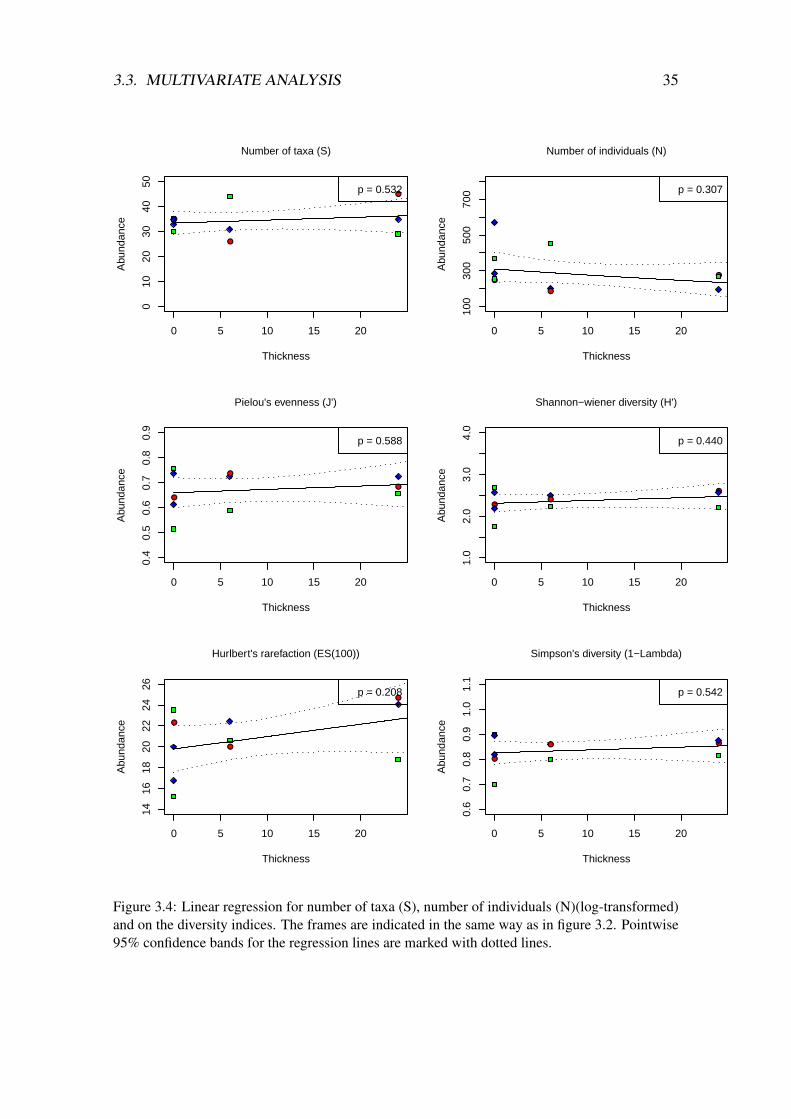
Shannon‘s diversity index ranged from 1.7 to 2.7, Pielou‘s evenness from 0.51 to 0.82,Simpson‘s from 0.69 to 0.89 and Hurlbert‘s rarefaction ranged from 15.22 to 24.7 (tableA.1 in appendix A and figure 3.1). Only two of the boxes had values below 18.5 for Hurl-bert’s rarefaction and both of these were surprisingly from the controls. Pielou’s evennessindex show a significant difference between the groups; there is a higher evenness in theestablished community at the experimental site, but also surprisingly higher (though notsignificant) evenness in the 24mm treatment compared to the 6mm treatment. There is awider range for the numbers for the diversity indices in the controls compared with theambient samples and the treatments. There are no significant results in the regressionanalysis on the diversity indices) (figure 3.4). Hurlbert’s rarefaction show a weak positivetrend as a function of increasing thickness layer of drill cuttings.
3.2.2 Faunal Composition
The ten most abundant taxa for each of the treatments and the ambient samples are listedin table 3.4. Most of the species are polychaetes with except for a few, one Echiuran(Echiurus echiurus), some Ophiurids and Calanoids. The most abundant taxon in theexperiment was the polychaet Polydora caulleryi, which comprised from 25% to almost30% of the abundance in the treatments, followed by Pseudopolydora pausibranchiata,Heteromastus filiformis and Prionospio steenstrupi. The ambient samples has a clearlydifferent composition with several species not found in the experiment (table 3.4). The tenmost abundant taxa in each of the samples are listed in figure A.2, in appendix A. Thereis a tendency for more dominance in the controls and the ambient samples, where the ten
30 CHAPTER 3. RESULTS
2460Ambient
0.90
0.85
0.80
0.75
0.70
1 - Lambda
Simpson
2460Ambient
0.85
0.80
0.75
0.70
0.65
0.60
0.55
0.50
J'
Pielous evennes
2460Ambient
2.8
2.6
2.4
2.2
2.0
1.8
H'
Shannon-wiener
2460Ambient
25.0
22.5
20.0
17.5
15.0
ES(100)
Hurlbert`s rarefaction
Figure 3.1: Simpsons diversity (1-Lambda), Pielou’s evenness index (J’), Shannons diversity exp(H’) and Hurlbert’s rarefaction (ES100) for the ambient samples and the experimental boxes. Box-plots with median, range, 1st(Q1) and 3rd(Q3) quartiles indicated.
3.3. MULTIVARIATE ANALYSIS 31
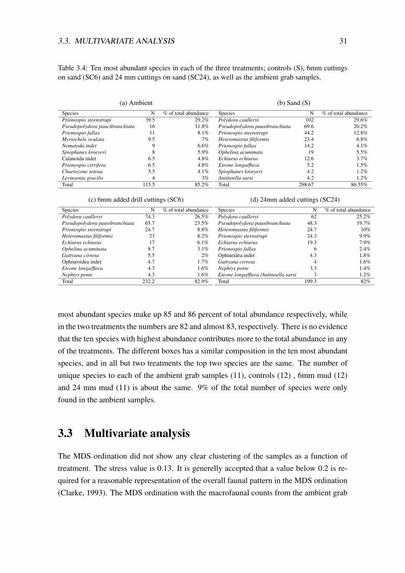
Table 3.4: Ten most abundant species in each of the three treatments; controls (S), 6mm cuttingson sand (SC6) and 24 mm cuttings on sand (SC24), as well as the ambient grab samples.
(a) AmbientSpecies N % of total abundancePrionospio steenstrupi 39.5 29.2%Pseudopolydora paucibranchiata 16 11.8%Prionospio fallax 11 8.1%Myriochele oculata 9.5 7%Nematoda indet 9 6.6%Spiophanes kroeyeri 8 5.9%Calanoida indet 6.5 4.8%Prionospio cirrifera 6.5 4.8%Chaetozone setosa 5.5 4.1%Levinsenia gracilis 4 3%Total 115.5 85.2%
(b) Sand (S)Species N % of total abundancePolydora caulleryi 102 29.6%Pseudopolydora pausibranchiata 69.6 20.2%Prionospio steenstrupi 44.2 12.8%Heteromastus filiformis 23.4 6.8%Prionospio fallax 14.2 4.1%Ophelina acuminata 19 5.5%Echiurus echiurus 12.6 3.7%Eteone longa/flava 5.2 1.5%Spiophanes kroeyeri 4.2 1.2%Antinoella sarsi 4.2 1.2%Total 298.67 86.55%
(c) 6mm added drill cuttings (SC6)Species N % of total abundancePolydora caulleryi 74.3 26.5%Pseudopolydora pausibranchiata 65.7 23.5%Prionospio steenstrupi 24.7 8.8%Heteromastus filiformis 23 8.2%Echiurus echiurus 17 6.1%Ophelina acuminata 8.7 3.1%Gattyana cirrosa 5.5 2%Ophiuroidea indet 4.7 1.7%Eteone longa/flava 4.3 1.6%Nephtys pente 4.3 1.6%Total 232.2 82.9%
(d) 24mm added cuttings (SC24)Species N % of total abundancePolydora caulleryi 62 25.2%Pseudopolydora pausibranchiata 48.3 19.7%Heteromastus filiformis 24.7 10%Prionospio steenstrupi 24.3 9.9%Echiurus echiurus 19.3 7.9%Prionospio fallax 6 2.4%Ophiuridea indet 4.3 1.8%Gattyana cirrosa 4 1.6%Nephtys pente 3.3 1.4%Eteone longa/flava /Antinoella sarsi 3 1.2%Total 199.3 82%
most abundant species make up 85 and 86 percent of total abundance respectively, whilein the two treatments the numbers are 82 and almost 83, respectively. There is no evidencethat the ten species with highest abundance contributes more to the total abundance in anyof the treatments. The different boxes has a similar composition in the ten most abundantspecies, and in all but two treatments the top two species are the same. The number ofunique species to each of the ambient grab samples (11), controls (12) , 6mm mud (12)and 24 mm mud (11) is about the same. 9% of the total number of species were onlyfound in the ambient samples.
3.3 Multivariate analysis
The MDS ordination did not show any clear clustering of the samples as a function oftreatment. The stress value is 0.13. It is generelly accepted that a value below 0.2 is re-quired for a reasonable representation of the overall faunal pattern in the MDS ordination(Clarke, 1993). The MDS ordination with the macrofaunal counts from the ambient grab

32 CHAPTER 3. RESULTS
●
●
●
0 5 10 15 20
05
1015
2025
30Ophelina acuminata
Thickness
Abu
ndan
ce
p = 0.002●
●
●
0 5 10 15 20
050
100
150
200
Polydora caulleryi
Thickness
Abu
ndan
ce
p = 0.441
●
●
●
0 5 10 15 20
050
100
150
Pseudopolydora pausibranchiata
Thickness
Abu
ndan
ce
p = 0.360
●
●
●
0 5 10 15 20
02
46
810
Antinoella sarsi
Thickness
Abu
ndan
cep = 0.484
●
●
●
0 5 10 15 20
05
1015
2025
30
Echiurus echiurus
Thickness
Abu
ndan
ce
p = 0.101
●
●
●
0 5 10 15 20
050
100
150
Prionospio steenstrupi
Thickness
Abu
ndan
ce
p = 0.932
Figure 3.2: Linear regression on log transformed faunal counts for the ten most abundant species.Frame A = red circles, frame B = green squares and frame D = blue diamonds. Pointwise 95%confidence bands for the regression lines are marked with dotted lines.

3.3. MULTIVARIATE ANALYSIS 33
● ●
●
0 5 10 15 20
020
4060
80
Heteromastus filiformis
Thickness
Abu
ndan
ce
p = 0.746
●
●●
0 5 10 15 20
010
2030
40
Prionospio fallax
Thickness
Abu
ndan
ce
p = 0.493
● ●
●
0 5 10 15 20
05
1015
Spiophanes kroyeri
Thickness
Abu
ndan
ce
p = 0.739
●
●
●
0 5 10 15 20
05
1015
Eteone longa/flava
Thickness
Abu
ndan
ce
p = 0.212
Figure 3.2: (continued)

34 CHAPTER 3. RESULTS
●
●
●
0 5 10 15 20
05
1015
2025
30Carnivore/Omnivore
Thickness
Abu
ndan
ce
p = 0.551
●
●
●
0 5 10 15 20
020
4060
8010
0
Sub−surface deposit feeders
Thickness
Abu
ndan
ce
p = 0.578
●●
●
0 5 10 15 20
050
100
200
Surface deposit feeders
Thickness
Abu
ndan
ce
p = 0.415
●
●
●
0 5 10 15 20
02
46
810
Suspension feeders
Thickness
Abu
ndan
cep = 0.532
● ●
●
0 5 10 15 20
050
100
150
200
Suspension/Surface deposit feeders
Thickness
Abu
ndan
ce
p = 0.939
Figure 3.3: Linear regression on log transformed faunal counts on feeding groups. The framesare indicated in the same way as in figure 3.2. Pointwise 95% confidence bands for the regressionlines are marked with dotted lines.
3.3. MULTIVARIATE ANALYSIS 35
●
●
●
0 5 10 15 20
010
2030
4050
Number of taxa (S)
Thickness
Abu
ndan
ce
p = 0.532
●●
●
0 5 10 15 20
100
300
500
700
Number of individuals (N)
Thickness
Abu
ndan
ce
p = 0.307
●
●
●
0 5 10 15 20
0.4
0.5
0.6
0.7
0.8
0.9
Pielou's evenness (J')
Thickness
Abu
ndan
ce
p = 0.588
●
●
●
0 5 10 15 20
1.0
2.0
3.0
4.0
Shannon−wiener diversity (H')
Thickness
Abu
ndan
cep = 0.440
●
●
●
0 5 10 15 20
1416
1820
2224
26
Hurlbert's rarefaction (ES(100))
Thickness
Abu
ndan
ce
p = 0.208
●
●●
0 5 10 15 20
0.6
0.7
0.8
0.9
1.0
1.1
Simpson's diversity (1−Lambda)
Thickness
Abu
ndan
ce
p = 0.542
Figure 3.4: Linear regression for number of taxa (S), number of individuals (N)(log-transformed)and on the diversity indices. The frames are indicated in the same way as in figure 3.2. Pointwise95% confidence bands for the regression lines are marked with dotted lines.
36 CHAPTER 3. RESULTS
samples combined with the counts from the experiment show two distinct groups, onegroup consisting of the two grab samples and one group consisting of the experimentalboxes (figure B.2, in appendix B). This shows a clear difference in the two subsets of sam-ples. MDS ordination as a function of frame show that the boxes in each of the frames aregrouped more closely than the boxes for each treatment (figure 3.6). MDS ordination asa function of treatment show no grouping, the boxes are randomly distributed in the plot(figure 3.5). The outlines show that none of the boxes from the different treatments aregrouped more closely than the others.
MDS ordination as a function of frame without the two most abundant species, Poly-
dora caulleryi and Pseudopolydora pausibranchiata was executed (figure B.3, appendixB). Without the two most abundant species the effect of frame changes, but is still present.In this plot frame A is more scattered, but frame B and D have about the same clustering.The same ordination was done as a function of treatment, which resulted in a differentcommunity structure, but no grouping of the frames according to treatment (figure B.1,in appendix B). To investigate the possibilty that the two most abundant species were re-sponsible for the frame effect another MDS was executed with only the two most abundantspecies, Polydora caulleryi and Pseudopolydora pausibranchiata (figure B.4, in appendixB). This plot shows no grouping of the samples neither according to frame nor accordingto treatment.
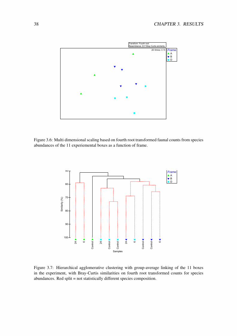
Cluster analysis based on Bray-Curtis similarities show the same groupings as theMDS as a function of frame (figure 3.7); the B and D frames are two almost separategroups with one box from frame D more closely related to frame B.

3.3. MULTIVARIATE ANALYSIS 37
Transform: Fourth rootResemblance: S17 Bray Curtis similarity
TreatmentControl246
2D Stress: 0.15
Figure 3.5: Multi dimensional scaling (MDS) based on fourth root transformed counts fromspecies abundances of the 11 experimental boxes as a function of thickness of drill cuttings. Thetreatments are outlined for illustration.
38 CHAPTER 3. RESULTS
Transform: Fourth root
Resemblance: S17 Bray Curtis similarity
Frame
A
B
D
2D Stress: 0.15
Figure 3.6: Multi dimensional scaling based on fourth root transformed faunal counts from speciesabundances of the 11 experiemental boxes as a function of frame.
24 6
Control
24
Control
Control
24 6
Control
Control 6
Samples
100
90
80
70
60
50
Similarity (%)
Frame
A
B
D
Figure 3.7: Hierarchical agglomerative clustering with group-average linking of the 11 boxesin the experiment, with Bray-Curtis similarities on fourth root transformed counts for speciesabundances. Red split = not statistically different species composition.
Chapter 4
Discussion
4.1 Effects of drill cuttings on benthic communities
Multivariate analysis of the faunal counts show no significant effects of the drill cuttings asa function of thickness layer of the cuttings added. The MDS analysis shows no groupingas a function of the treatment (figure 3.5). The regression analysis shows a weak tendencyto lower abundance as a function of the thickness layer of the drill cuttings.
This study provides no evidence that settling communities are sensitive to WBM cut-tings. This is in contrast to a related mesocosm experiment (Trannum et al, 2009)(alsoin PEIOFF-FAME) who found effects of WBM drill cuttings. These results indicatesthat living communities “buried” by WBM drill cuttings are more sensitive to this kindof contamination. The two types of experiments are widely different; in a recolonizationexperiment the sediment is defaunated, whereas in the mesocosm experiment the purposeis to imitate already established communities that are “buried” in drill cuttings. It is notunlikey that natural variation might cover negative effects of the drill cuttings in the field,since there was an effect in the mesocosm experiment, negative effects in the other partof the experiment (fine sediment) and a negative tendency in my part of the experiment.
My results are in compliance with findings of Daan and Mulder (1993). They foundno adverse effects of WBM-cuttings one year after dumping of WBM cuttings, even asclose as 25 m from the former discharge site. Recent field and laboratory studies tend toconfirm these results. Benthic fauna are not harmed by drill cuttings from WBM, sincethe exposure from drill cuttings from WBM in a oil field is of short duration and thecuttings are rapidly diluted. Impacts of WBM are limited to 100 m within the platformand recovery is well within one year. However, effects are more severe if released to;coastal areas, deep-water environments or low-energy habitats (Neff, 2005). In many of
39

40 CHAPTER 4. DISCUSSION
the cases where effects of WBM have been observed one has not been able to attributethese effects to WBM with certainty, because of previous drilling with OBM in the samearea (Daan and Mulder, 1993).
Bakke et al (1986) performed an experiment with four types of drill cuttings; WBM,LAC (low aromatic oil based), DOC (diesel oil based mud, washed wih diesel oil) andBRI-cuttings (cuttings from drilling with diesel oil based mud compressed into solid bri-quettes). As expected there were large differences in response between the oil and non-oil cuttings, with significant effects only in the sediment treated with oil based cuttings.There was a slightly stronger negative trend in this experiment compared to my experi-ment (Bakke et al, 1986). With the restrictions for OBM that came in 1993 there was aneed to improve the technical properties of WBM, since OBM was preferred due to itssuperior properties. It is reasonable to assume that the composition of WBM has changedbecause of this need. The stronger trend in Bakke et al (1986)’s experiment can possiblybe explained by the the fact that the composition of WBM might have changed (T Bakke2010, pers. com). My experiment differed in having higher number of species per boxat the same stage (after 6 months). There were on average 34 species per box in my ex-periment as opposed to about 22 per box in Bakke et al (1986). One possible explanationfor this difference is that there were fewer species identified to the species level (T Bakke2010, pers. com.).
Berge (1990) also did an experiment in the Oslofjord, but this was with sedimentstreated with crude oil. He did the experiment in two fjords with unequal eutrophicationstatus, Raunefjord in western Norway in addition to the Oslofjord. The eutrophicatedOslofjord was little affected by the oil, while there was a clear reduction of species inRaunefjord. The possible explanation given for this result is that communities with fewspecies, low diversity, high dominance and high production rates are more stress tolerant(they have a higher resilience) than more complex systems (Jernløv and Rosenberg, 1976).From these criteria the fauna found in my experiment does not have the characteristics fora resilient community, although the Oslofjord is described as one by the author above.The fauna in the ambient samples has many species, high diversity and low dominance.No measurements for production were made in my experiment, hence there is no value forthis factor. The difference between the fauna in Berge (1990) and my experiment can beexplained by the change in eutrophication status in the Oslofjord since 1990 (Magnussonet al, 1997). It is difficult to predict how resilient the Oslofjord is today. However, therehas been an overall improvement of the pollution situation in the Oslofjord since 1990.The fauna in the outer Oslofjord was surveyed by Niva in 2008, and the report showsa positive trend for the fauna in the outer Oslofjord, although Shannon-Wiener diversity
4.1. EFFECTS OF DRILL CUTTINGS ON BENTHIC COMMUNITIES 41
index (H’) and Hurlbert’s rarefaction (ES(n)) has not changed systematically. One stationin the survey is located right before the Oslofjord widens (Walday et al, 2009). Thisstation is located further out in the fjord from the experimental site. However, assumingsometimes inward directed currents the, community in my experiment may have receivedsome of its recruits from the outer part of the Drøbak strait. 70% of the species present inthe recruiting assemblages were not found in the adjacent seabed, indicating significantnonlocal recuitment.
Another factor is that the experimental site in Berge (1990)’s experiment was in theinner Oslofjord (Berge et al, 1987), which is known to be more polluted than the outerpart. The lacking effect from exposure of oil in the experiment in 1990 may not be com-parable with the experiment with WBM cuttings from 2007 in the same fjord, becauseof the improved environmental conditions and the following positive trend for the fauna.However, the improved conditions might have made the fauna in the Oslofjord less robusttoday present, so that it would be more likely to observe an effect of the drill cuttings.
4.1.1 Effects on faunal diversity
The diversity indices show that there is no effect of the drill cuttings on the diversity (fig-ure 3.1 and 3.4). The only index with significant differences are the Pielou’s evennessindex, where the ambient grab samples have a higher evennes. This is expected sincethe ambient samples are from mature communities. It is more surprising that the otherdiversity indices does not differ more, since a mature community is expected to have ahigher diversity (Margalef, 1963). The values for Hurlbert’s rarefaction are slightly higherin the samples with 24 mm added drill cuttings, which indicates a positive relationshipbetween the added cuttings and the number of species, but this is not statistically signif-icant. This result is unexpected and difficult to explain. Such high values are associatedwith a healthy fauna (Molvær et al, 1997), wich is an indication that the community is notpolluted and not affected by the drill cuttings added.
4.1.2 Effects on faunal composition
The composition of the most abundant species (figure 3.4) supports that the drill cuttingshave no significant effect on the settling of the benthic community in my experiment,since the composition of the ten most abundant species are similar in the treatments andthe control. The species Polydora caulleryi and Pseudopolydora pausibranchiata werethe two most abundant species in all except for two boxes. The rest of the species variedmore.

42 CHAPTER 4. DISCUSSION
Ophelina acuminata was the only species with significantly lower abundance as afunction of cuttings added. According to literature this species is sensitive to pollution(Rygg, 1985) and it is not surprising that we see a negative effect of the drill cuttings onthis species.
Polychaeta was the most abundant group in the experiment. This is in compliance withother sudies of recruiting soft-sediment assemblages (Berge, 1990; Olsgard, 1999; Tran-num et al, 2004). They found that polychaetes was the most abundant group, independentof depth and habitat and treatment.
Polydora Caulleryi was the most dominating species in many of the boxes in myexperiment, independent of treatment. This species is known to often be one of the firstcolonizers in a succession. Polydora has a flexible life history strategy and a short lifecycle which makes it a suitable colonist. (Gray and Elliott, 2009).
As mentioned in section 1.3, the larve of opportunistic species have little preferencesfor substratum for settlement. Members of the family Spionidae, often the genus Polydora
are the first to settle. Many of the most abundant species in this experiment are known tobe opportunistic, which could partly explain the lack of difference between the test boxesand the control boxes. If the experiment had lasted longer, it is possible that larvae of moreK-selected species would react differently to the exposure of drill cuttings. If “conditions”fail to improve (in the case where drill cuttings could affect K-selected species), the r-selected species may not be replaced by K-selected species (Gray and Elliott, 2009). It ispossible that a negative effect of the drill cuttings would appear at a later stage.
4.2 Effects of frame location
The MDS ordination shows a weak but clear grouping as a function of frame (figure 3.6).Some of the plots in the regression analysis stand out because the controls have a largerrange in the observations (figure 3.2, 3.3 and 3.4). This applies to the following plots: Pri-
ononospio steenstrupi, Prionospio fallax, Spiophanes kroyeri, Eteone longa/flava, sub-surface deposit feeders, suspension feeders, total abundance (N) and Pielou’s evennessindex. It looks like there is a pattern in the observations, because there is a preponderanceof observations with high abundance by blue diamonds (= frame D). Frame D was theframe that was placed on the opposite side of the fjord, away from the frame A and B. Apossible explanation for the preponderance may be a greater supply of larvae on the sideof the fjord where frame D was placed. One possible explanation is that the supply oflarvae for frame D could have come more from the outer Oslofjord than for frame A andB. Hydrodynamics and natural heterogenity can partly be responsible for this difference

4.3. ENVIRONMENTAL VARIABLES AS EXPLANATORY FACTORS 43
(Bourget and Harvey, 1998; Morrisey et al, 1992).
When removing the two most abundant species (both overall and most of the boxes),Polydora caulleryi and Pseudopolydora pausibranchiata from the MDS-ordination, theeffect of frame became much weaker (figure B.1, in appendix B). To test if these twospecies alone were responsible for the effect of frame, another MDS-plot with only thesetwo species was made (figure B.4, in appendix B). This MDS did not show an effect offrame, hence these two species cannot be accounted for the frame effect in the originalMDS-plot.
4.3 Environmental variables as explanatory factors
4.3.1 Total organic carbon (TOC)
Since total organic carbon for the drill cuttings and the test sediment were not measuredin this experiment, values from (Trannum et al, 2009) and (Olsgard, 1995) are used forcomparison. The same type of drill cuttings were used in my experiment as in Trannum’smesocosm experiment and the samples for the test sediment was taken in the same area asone of the stations in Olsgard’s survey from 1993. The TOC measured in the drill cuttingswas 0.8 % (Trannum et al, 2009) and the TOC value from the corresponding station in(Olsgard, 1995) was 1.9 %. The measured values for TOC are not particularly differentand both of the values are well within the criteria for a healthy bottom fauna determinedby Klif (earlier SFT) (Molvær et al, 1997).
4.3.2 Grain size
The sandy sediment and the drill cuttings differ in grain size, while the fine sedimentand the drill cuttings are only slightly different in sediment grain size. If grain size is animportant factor for settling and recolonization after disturbance from WBM drill cuttings,we should have seen an effect on the fauna in the experiment. Grain size is considered animportant factor in structuring benthic communities (Grebmeier et al, 1989). The authorsfound that lower diversity correlated with an increase in fine sand fractions. However,my results does not correspond with these findings. Preliminary results from the finesediments show an effect from the drill cuttings on the fauna (Trannum, unpublishedresults). Based on the grain size factor it is unexpected that the results show an effect inthe fine sediment, while there was only seen a negative effect of the drill cuttings on onespecies in the coarse sediment (my part of the experiment).
44 CHAPTER 4. DISCUSSION
The level of no observable effect, PNEC is a central part of the EIF (EnvironmentalImpact Factor) which again is a part of ERMS (Environmental Risk Management System)that is developing for offshore drilling activities. Default values for PNEC are at presentused to estimate effects of drill cuttings (Olsgard et al, 2005). All PNEC-values are atcurrently independent of the biota present in the sediment. A 21% change in mediangrain size is the PNEC-value determined by Leung et al (2005). The change in grain sizein my experiment is more than the PNEC-value of 21% change (a reduction from 65m µ
to 10.9 mµ). It is also more than the Hazardous level (HL50), wich is 17.8 µm determinedby (Smit et al, 2008). On the basis of these numbers and and the results from the wholeexperiment it is surprising that no effect of the drill cuttings was found, particularly whenwe know from literature that grain size is an important for the settlement of benthic larvae(Grebmeier et al, 1989).
4.3.3 Oxygen penetration
There is no significant reduction of the oxygen penetration depth as a function of increas-ing layer thickness of drill cuttings (table 3.1), although there is a decreasing trend. Inmesocosm experiments with WBM cuttings, Trannum et al (2009) found that the oxygenpenetration depth decreased as a function of layer thickness of the drill cuttings becauseof oxygen depletion. In their experiment, the test sediment boxes (2.1% ) had a higherTOC content than the boxes with drill cuttings (0.8%). The author suggest that the organiccarbon present in the cuttings was more degradeable than the TOC in the test boxes. Inaddition, decay of dead fauna in the treatments with drill cuttings may have contributedto the decreased oxygen penetration depth (Trannum et al, 2009). It is possible that theoxygen level in the boxes in my experiment with drill cuttings was initially lower, butthis situation might have gradually improved in the field because of the water currentscirculating oxygen to the boxes (H Trannum 2010, pers. com.).
4.4 Conclusions
No clear relationship between the dose of WBM cuttings and the effect on settling of thebenthic ecosystem on coarse sediments was found, but there was a clear negative trend.It is not impossible that natural variation covers an effect of the drill cuttings in the field.The environmental variables explained to some extent this result. Oxygen penetrationdepth supported this result, but grain size deviated with an unexpected result, i.e. moresignficant effects on fine sediment despite the fact that the fine sediments and the drill

4.5. LIMITATIONS 45
cuttings have a more similar grain size than the cuttings and the coarse sediment. Otherunexpected results that are difficult to explain are the higher variation in abundances inthe control trays and the higher diversity (Hurlbert’s rarefaction) in the treatments withdrill cuttings. It is possible that the picture will change when all the results from theexperiment is in place. It was not possible to include the rest of the results because ofthe limited time frame of the master thesis. For further research it would be interestingto do an experiment in a location that is known to have sensitive species. This would behighly relevant since it is not yet settled whether or not oil should be recovered from thevulnerable areas in Northern Norway.
4.5 Limitations
Fundamental to ecology is how populations, communities, and the processes that influ-ence them vary with changes in spatial and temporal scale. This is important to have inmind, because field experiments can only feasibly be conducted at small spatial scales(Thrush et al, 1996). The time frame is also usually a limiting factor.
To what extent can we use small scale experiments to predict larger scale responses?Zajac et al (1998) suggests that this may not be possible, because of the mix of factorscontrolling successive processes at different spatial scales may be fundamentally differ-ent. However, definitive causal relationships between the presence of contaminants andtheir effects can only be shown by manipulative experiments (Underwood and Peterson,1988). Manipulative field experiments are particurlary well suited for studying recruit-ment of benthic communities. This is becoming an increasingly more common methodfor studying processes and variables that influence biological patterns of distribution insoft-sediments (Olsgard, 1999; Trannum et al, 2004; Olsgard et al, 2005).
Potential errors can be made in several stages in the process. The experimental designmay potentially contain weaknesses; four frames were deployed on two different locationsnot far from each other, far enough to be true replicates, but close enough that an effectof frame/location should be avoided. A weak frame effect was present, but this does notnecessarily mean that there is a weakness in the set-up of the experiment. The resultmay be an indication that even on such small scales, the communities have a differentcomposition. This may be because of different recruitment potential (Morrisey et al,1992). The dead fauna in the sediment collected for the experiment was not removed,and could potentially have influenced recolonisation. Another possible weakness of theexperiment is that we cannot be sure that the thickness of the drill cuttings stayed thesame troughout the experiment.

46 CHAPTER 4. DISCUSSION
The frames were placed 20 cm above the seabed, but since most macrofauna is dis-persed as pelagic larva, this will probably not represent a major obstacle for colonizationthrough settlement. Previous studies on recolonization show that pelagic larval recruit-ment accounts for between 70% and 90 % of all individuals (McCall, 1977; Santos andSimon, 1980; Diaz-Castaneda et al, 1993).
One could possibly argue that the experiment should have lasted longer to observeeffects on a more mature community. Bakke et al (1986) showed that benthic communitiescan be initially moderately affected by drill cuttings from OBM and then after two yearscome to a total collapse. The reference and the WBM followed one another through theexperiment and as in my experiment there was no significant effect of the WBM drillcuttings. Since there was a longer time frame in this experiment it was more suitable topredict development in the community over time (Bakke et al, 1986). A scenario similarto that for OMB cuttings is probably not likely with WBM cuttings, even with a longertime frame since they are known to have less effect on benthic fauna (Daan and Mulder,1993; Olsgard and Gray, 1995; Neff, 2005).
The identification process is also a stage where potensial mistakes can be made. AsI am an unexperienced taxonomist, there is a potential risk that I might make mistakes,especially in the beginning. Although not systematically, a significant amount of reidenti-fication was carried through in cases where it was clear that specimens were misidentified.A lot of the identification work was also controlled by a supervisor. Possible errors madeduring identification can have serious consequences for the result and the reliability ofthe experiment. Some errors will affect the result, others will not. Mislabeling an entirespecies will not affect the result because statistics are independent on species names. Itwill only affect the result when looking for explanations for the result in the ecology ofspecies or groups of species. Mislabeling some specimens of a species could affect theresult if this applies to many animals. In my results, the chance that there are large errorsis considered low, because of the consistenct in the results from the whole experiment.The result from the ten most abundant species in all the boxes (figure A.2, in appendixA) can possibly indicate that there are no large errors in the identification because of theoverall consistency. The Capitellides may be a possible source for errors in the identi-fication. They are very small and it is difficult to se all the setae. Since there is a largepredominance of Heteromastus filiformis and little deviation from the fine material it ismost likely correct on the coarse material as well.
There were only taken two ambient grab samples. This is obviously to few replicatesto do proper statistics, but the ambient samples are still included in the box plots for illus-tration of the difference between the adjacent seabed and the experimental community.

4.5. LIMITATIONS 47
Both parametric and non-parametric statistics are used in the analysis of the fauna inthe experiment. Non-parametric methods are based on fewer assumptions and it is notpossible to make a direct comparison of the results. However, it is possible to discuss thevalidity of the assumptions for both the parametric and non-parametric methods. Hence;how well the parametric method fits for the purpose and the corresponding: how well thenon-parametric method acts for the purpose. This will not be discussed her as it is beyondthe scope of this thesis.

48 CHAPTER 4. DISCUSSION
Bibliography
Christensen J M, Larsen S and Nystrøm B O. (1978). Muslinger. J.W. Cappelens forlagAS, 125s.
Enckell P H (1998). Kraftdjur. Bokforlaget Signum, Lund.
Hayward P J, Ryland J S (1994) Handbook of the marine fauna of North-West Europe.Oxford University Press
Holthe T (1986) Polychaetha. Terebellomorpha. Marine invertebrates of Scandinavia 7.Universitetsforlaget
Kirkegaard J B (1992) Havbørsteorme I. Errantia. Danmarks fauna 83. Dansk Naturhis-torisk Forening.
Kirkegaard J B (1992) Havbørsteorme II. Sedentaria. Danmarks fauna 86. DanskNaturhistorisk Forening.
Lincoln RJ, (1979). British marine amphipods. Gammaridea. British Museum (NaturalHistory), London
Mortensen, T. (1924). Pighude. Danmarks Fauna 27: 1-274.
Newell G E and R C (1963) Marine Plankton. A practical guide. Hutchinson educa-tional.
Pleijel F (1993) Polychaetha. Phyllodocidae. Marine Invertebrates of Scandinavia 8.Universitetsforlaget.
Rainer S F (1991). The genus Nephtys (Polychaetha: Phyllodocida) of northern Europde:a review of species, including the description of N. pulchra sp. n. and a key to theNephtyidae. Helgolander meeresuntersuchen 45, 65-96.
Sars GO, (1890) (reprinted 1966). An Account of the Crustacea of Norway. Vol. I.Amphipoda. Universitetsforlaget, Bergen and Oslo
Sars GO, (1900). An Account of the Crustacea of Norway. Vol. III. Cumacea. Christia-nia
Tebble N, (1966). British bivalve seashells. Trustees of the British Museum (NaturalHistory), 212 s.
49

50 CHAPTER 4. DISCUSSION
Tebble N and Chambers S (1982). Polychaetes from Scottish Waters. A guide to identi-fication. Part I Family Polynoidae. Royal Scottish Museum Studies.
Todd C D, Laverack M S and Boxshall G A (1996). Coastal marine zooplankton. Apractical manual for students. Cambridge University Press.
Wesenberg-Lund, E. (1939). Danmarks Fauna. Pølseorme (Gephyrea) Sipunculider,Priapulider, Echiurider. G.E.C. Gads forlag, København. 59 pp.

References
Arntz W (1977) Results of an ’unsuccessfull’ benthos cage predation experiment (WesternBaltic). pp. 31-34. In: Keegan, BF, P O’Ceidagh, and PJS Boaden (eds.), Biology ofbenthic organisms. Pergamon Press, New York.
Bakke T, Green N, Næs K, Pedersen A (1986) Drill cuttings on the sea bed. Phase 1and 2. Field experiment on benthic recolonization and chemical changes in response tovarious types and amounts of cuttings. Tech. rep., NIVA
Bellan G, Reish D, Foret J (1972) The sublethal effects of detergent on the reproduction,development, and settlement in the polychaetous annelid Capitella capitata. MarineBiology 14:183–188
Berge J (1990) Macrofauna recolonization of subtidal sediments. Experimental studieson defaunated sediment contaminated with crude oil in two Norwegian fjords with un-equal eutrophication status. I. Community responses. Marine Ecology Progress Series68:103–115
Berge J, Lichtenthaler R, Oreld F (1987) Hydrocarbon Depuration and Abiotic Changesin Artificially Oil Contaminated Sediment in the Subtidal. Estuarine, Coastal and ShelfScience 24:567–583
Berge JA (1993) The effect of treated drill cuttings on benthic recruitment and communitystructure- and experimental study on a natural seabed. Tech. Rep. O-91090, NIVA
Bourget E, Harvey M (1998) Spatial analysis of recruitment of marine invertebrates onarborescent substrata. Biofouling 12(1-3):45–55
Burke R (1986) Pheromones and the gregarious settlement of marine invertebrate larvae.Bulletin of Marine Science 39:323–331
Butman C, Grassle J, Webb C (1988) Substrate choices made by marine larvae in stillwater and in a flume flow. Nature 333(23)
Caenn R, Chillingar GV (1996) Drilling fluids: State of the art. Journal of PetroleumScience and Engineering 14(3-4):221 – 230
Clarke K (1993) Non-parametric multivariate analyses of changes in communtiy struc-ture. Aust J Ecology 18:117–143
51

52 REFERENCES
Clarke R, Warwick R (2001) Change in marine communities: an approach to statisticalanalysis and interpretation, 2nd edition.
Connel J, Slatyer R (1977) Mechanism of succession in natural communities. AmericanNaturalist 111:1119–1144
Cripps S, Picken G, Aabel J, Andersen O, Heyworth C, Jakobsen M, Kristiansen R,Marken C, Paulsen J, Shaw D, Annand A, Jacobsen T, Henriksen I (1998) Disposalof oil-based cuttings. Tech. Rep. RF-98/097, Rogaland Research
Daan R, Mulder M (1993) A study on possible environmental effects of a WBM cuttingdischarge in the North Sea, one year after termination of drilling. Tech. Rep. 1993-16,Nederlands Instituut voor Onderzoek der Zee
Davies J, Addy J, Blackman R, Blancards J, Ferbrache J, Moore D, Sommerville H,Whitehead A, Wilkinson T (1984) Environmental effects of the use of Oil-based drillingmuds in the North Sea. Marine Pollution Bulletin 15(10):363–370
Diaz-Castaneda V, Frontier S, Arenas V (1993) Experimental re-establishment of a softbottom community: Utilization of multivariate analyses to characterize different ben-thic recruitments. Estuarine, Coastal and Shelf Science 37(4):387–402
Eckman JE (1996) Closing the larval loop: linking larval ecology to the population dy-namics of marine benthic invertebrates. Journal of Experimental Marine Biology andEcology 200(1-2):207 – 237
Eleftheriou A, Moore D (2005) Macrofauna techniques. In: Methods for the study ofmarine benthos., Blackwell Science.
Eyster L, Pechenik J (1987) Attachment of Mytilus edulis L. larvae on algal and byssalfilaments is enhanced by water agitation. Journal of Experimental Marine BiologicalEcology 114:99–110
Fager E (1964) Marine sediments: effects of a tube-building polychaete. Science36:1288–1300
Gallagher E, Jumars P, Trueblood D (1983) Facilitation of soft-bottom benthic successionby tube builders. Ecology 64:1200–1260
Grassle J, Grassle J (1974) Opportunistic life histories and genetic systems in marinebenthic polychaetes. Journal of Marine Research 32:253–284
Gray J (1981) The ecology of marine sediments: an introduction to the structure andfunction of benthic communities. Cambridge University Press.
Gray J, Elliott M (2009) Ecology of Marine Sediment - From Science to Management.,2nd edn. Oxford university press

REFERENCES 53
Gray JS, Bakke T, Beck HJ, Nilssen I (1999) Managing the Environmental Effects ofthe Norwegian Oil and Gas Industry: From Conflict to Consensus. Marine PollutionBulletin 38(7):525 – 530
Grebmeier J, Feder H, McRoy C (1989) Pelagic-benthic coupling on the shelf of thenorthern Bering and Chukchi Seas. 11. Benthic community structure. Marine EcologyProgress Seriess 51:253–268
Gunther C (1992) Dispersal of intertidal invertebrates: a strategy to react to disturbancesof different scales? N J Sea Res 30:45–56
Hinwood J, Potts A, Dennis L, Carey J, Houridis H, Bell R, Thompson J, Boudreau P,Ayling A (1994) Environmental implications of offshore oil and gas development inAustralia - drilling activities. Tech. rep., Australian petroleum association (APEA), En-ergy research and development corporation (ERDC) pp. 123-206
Holdway D (2002) The acute and chronic effects of wastes associated with offshore oiland gas production on temperate and tropical marine ecological processes. Marine Pol-lution Bulletin 44:185–203
Hurlbert S (1971) The nonconcept of species diversity: a critique and alternative param-eters. Ecology 52:577–586
Jablonski D, Lutz R (1983) Larval ecology of marine benthic invertebrates: paleobiolog-ical implications. Biol Rev Camb Philos Soc 58:21–89
Jensen T, Palerud R, Olsgard F, Bakke S (1999) Fate and effects of synthetic drillingmuds in the environment. Biological monitoring, long-term effects of oil and producedwater, chemicals and oil-spill preparedness – Technical report to the Ministry of Oiland Energy. Tech. Rep. 99/3507, Det Norske Veritas
Jernløv A, Rosenberg R (1976) Stress tolerance of ecosystems. Environmental conserva-tion 3:43–46
Klif (2009) Miljømal offshore bør omfatte radioaktivitet. URL: http://www.klif.no/no/Aktuelt/Nyheter/2009/Januar-2009/Miljomal-offshore-bor-omfatte-radioaktivitet
Klif (2010) Klima- og forurensningsdirektoratets vurdering av maloppnaelse for nullut-slippsarbeidet. Tech. rep., Klima og forurensningsdirektoratet, Klif
Leung K, Bjørgesæter A, Gray J, Li W, Lui G, Yuan W, Lam P (2005) Deriving sedimentquality guidelines from field-based species sensitivity distributions. Environmental Sci-ence Technology 39:5148–5156
Levin L (1985) Dispersion, feeding behaviour and competition in two spionid poly-chaetes. Journal of Marine Research 65:107–119
Lu L, Wu R (2000) An experimental study on recolonization of marine macrobenthos indefaunated sediment. Marine Biology 136:291–302
54 REFERENCES
Luckenbach M (1984) Settlement and early postlettlement survival in the recruitment ofMulinia lateralis (Bivalvia- Probability of settling and gregourius behaviour). MarineBiology Progress Seriess 17:245–250
Magnusson J, Gjøsæther J, Knutzen J, Lømsland E, Johnsen T, Schram T, Sollie A (1997)Overvakningssituasjonen i indre Oslofjord 1997. Tech. Rep. 732/98, NIVA
Margalef R (1963) On certain unifying principles in ecology. The American Naturalist97(897):357–374
Marsden J, Conlin B, Hunte W (1990) Habitat selection in the tropical polychaete Spiro-branchus giganteus. II. Larval preferences for corals. Marine biology 104:93–99
McCall P (1977) Community patterns and adaptive strategies of the infaunal benthos ofLong Island Sound. Journal of Marine Research 35:221–266
Menzie C (1984) Diminishment of recruitment: a hypothesis concerning impacts on ben-thic communities. Marine Pollution Bulletin 15:127–128
Molvær J, Knutzen J, Magnusson J, Rygg B, Skei J, Sørensen J (1997) Classification ofenvironmental quality in fjords and coastal waters. A guide. Tech. rep., NIVA, publisherSFT (now Klif)
Morrisey D, Howitt L, Underwood A, Stark J (1992) Spatial variation in softsedimentbenthos. Marine Ecology Progress Series 81:197–204
Neff (1987) Offshore oil and gas development activities potentially causing long-termenvironmental effects, Elsevier applied science publishers, London, chap Long termeffects of offshore and gas development, pp 149–174
Neff J (2005) Composition, Environmental fates, and biological effects of water baseddrilling muds and cuttings discharged to the marine environment: A synthesis and An-notated Bibliography. Tech. rep., Battelle, The business of innovation
Neff J, McKelvie S, Ayers R (2000) Environmental impacts of synthetic based drillingfluids. OCS Study 2000-64, U.S. Dept. of the Interior, Minerals Management Service,Gulf of Mexico OCS Region, New Orleans, LA
OLF (2009) Leting etter olje og gass. URL: http://www.olf.no/oljefakta/leting-etter-olje-og-gass-article570-166.html
Olive P, Clark R (1978) Physiology of Annelids, Academic press, chap The physiologyof reproduction, pp 271–368
Olsen G, Carrol M, Renaud P, Ambrose W, Olssøn, Carrol J (2007) Benthic communityresponse to petroleum-associated components in Arctic versus temperate marine sedi-ments. Marine Biology 151(6):2167–2176
REFERENCES 55
Olsgard F (1995) Overvaking av forurensningssituasjonen i indre Oslofjord. Un-dersøkelser av bløtbunnsfauna 1993. Tech. Rep. 622/95, University of Oslo
Olsgard F (1999) Effects of copper contamination on recolonisation of subtidal marinesoft sediments - an experimental field study. Marine Pollution Bulletin 38(6):448 – 462
Olsgard F, Gray J (1995) A comprehensive analysis of the effects of offshore oil and gasexploration and production on the benthic communities of the Norwegian continentalshelf. Marine Ecology Progress Series 122:277–306
Olsgard F, Schaanning M, Hylland K, Trannum H, Carrol J, Dahle S, Olsen G, Rye H,Gray J, Bjørgesæter A, Neff J, Kingston P (2005) Project description: Parameterisationof the Environmental Impacts of Bottom Fauna of Water-based Drilling Fluids andCuttings -Field and Mesocosm Experiments (PEIOFF-FAME). Application to NFR.
Pawlik J (1992) Chemical ecology of the settlement of the marine benthic invertebrates.Oceanographical Marine Biology Annual Review 30:273–335
Pearson T, Rosenberg R (1978) Macrobenthic successsion in relation to organic enrich-ment and pollution of the marine environment. Oceanography Marine Biology AnnualReview 16:229–311
Pechenik J (1999) On the advantages and disadvantages of larval stages in benthic marineinvertebrate life cycles. Marine Ecology Progress Series 177:269–297
Pielou E (1966) The measurement of diversity in different types of biological collections.Journal of Theoretical Biology 13:131–144
Probert P (1984) Disturbance, sediment stability and trophic structure of soft-bottom com-munities. Journal of Marine Research 42:893–921
Quian P (1999) Larval settlement of polychaetes. Hydrobiologia 402:239–253
Renaud P, Jensen T, Wassbotten I, Mannvik H, Botnen H (2008) Offshore sediment mon-itoring on the norwegian shelf. a regional approach 1996-2006. Tech. Rep. 3487-003,Akvaplan-niva
Rhoads D, Young D (1970) The influence of deposit-feeding organisms on sediment in-stability and community trophic structure. Journal of Marine Research 28(2):150–178
Rhoads D, Aller R, Goldhaber M (1977) The influence of colonizing benthos on physicalproperties and chemical diagenesis of the estuarine seafloor. In: Coull, B. C. (ed.),Belle Baruch symposium on the ecology of marine benthos. University of South Car-olina Press, Columbia, South Carolina.
Rygg B (1985) Distribution of species along pollution-induced diversity gradients in ben-thic communities in Norwegian fjords. Marine Pollution Bulletin 16(12):469 – 474
Sanders H (1968) Marine benthic diversity. Am Nat 102:243–282

56 REFERENCES
Sanders H, Goudsmit E, Mills E, Hampson G (1962) A study of the intertidal fauna ofBarnstable Harbor, Massachusetts. Limnology and Oceanography 7:63–79
Santos S, Simon J (1980) Marine soft-bottom community establishment following annualdefaunation: Larval or adult recruitment? Marine ecology progress series 2:235–241
Schaanning M, Bakke T (2006) Remediation of sediments contaminated with drill cut-tings. A review of field monitoring and experimental data for validation of the ERMSsediment module. Tech. Rep. 5188-2006, NIVA
Schaanning MT, Trannum HC, Øxnevad S, Carroll J, Bakke T (2008) Effects of drillcuttings on biogeochemical fluxes and macrobenthos of marine sediments. Journal ofExperimental Marine Biology and Ecology 361(1):49 – 57
Shannon C, Weaver W (1963) The mathematical theory of communication. University ofIllinois Press, 117pp
Simpson E (1949) Measurement of diversity. Nature 163:688–688
Smit M, Holthau K, Trannum H, Neff J, Kjeilen-Eilertsen G, Jak R, Singsaas I, HuijbregtsM, Hendriks A (2008) Species sensitivity distributions for suspended clays, sedimentburial, and grain size in the marine environment. Environmental Toxicology and Chem-istry 27(4):1006–1012
Smith C, Brumsickle S (1989) The effects of patch size and substrate isolation on colo-nization modes and rates in an intertidal sediment. Limnol Oceanogr 34(7):1263–1277
Stark J, Snape I, Riddle M (2003) The effects of petroleum hydrocarbon and heavy metalcontamination of marine sediments on recruitment of Antarctic soft-sediment assem-blages: a field experiment investigation. Journal of Experimental Marine Biology andEcology 283:21–50
Tagatz M, Tobia M (1978) Effect of Barite (BaSO4), on development of estuarine com-munities. Estuarine and Coastal Marine Science 7:401–407
Thistle D (1981) Natural physical disturbances and communities of marine soft-bottoms.Marine Ecology Progress Series 6:223–228
Thrush S (1991) Spatial patterns in soft-bottom communities. Trends in Ecol Evol 6:75–79
Thrush S, Whitlatch R, Pridmore R, Hewitt J, Wilkinson VCM (1996) Scale-dependentrecolonization: The role of sediment stability in a dynamic sandflat habitat. Ecology77(8):2472–2487
Trannum H, Nilsson H, Schaanning M, Øxnevad S (2009) Effects of sedimentation fromwater-based drill cuttings and natural sediment on benthic macrofaunal communitystructure and ecosystem processes. Journal of Experimental Marine Biology and Ecol-ogy 383(2):111–121

REFERENCES 57
Trannum HC, Olsgard F, Skei JM, Indrehus J, Øveras S, Eriksen J (2004) Effects ofcopper, cadmium and contaminated harbour sediments on recolonisation of soft-bottomcommunities. Journal of Experimental Marine Biology and Ecology 310(1):87 – 114
Underwood A, Peterson C (1988) Towards an ecological framework for investigating pol-lution. Marine Ecology Progress Seriess 46:227–234
Walday M, Naustvoll L, Nilsson H, Rygg B, Selvik J, Sørensen K (2009) Overvaking avytre Oslofjord 2008. Tech. Rep. 5818-2009, NIVA
Watzin M (1983) The effects of meiofauna on settling macrofauna: Meiofauna may struc-ture macrofaunal communities. Oecologica 59:163–166
Wei-Jun C, Sayles F (1996) Oxygen penetration depth and fluxes in marine sediments.Marine Chemistry 52:123–131
Woodin S (1976) Adult-larval interactions in dense faunal assemblages: patterns of abun-dance. Journal of Marine Research 34:25–41
Zajac R, Whitlach R, Thrush S (1998) Recolonization and succession in soft-sediment infaunal communities: the spatial scale of controlling factors. Hydrobiologia375/376:227–240

58 REFERENCES

Appendix A
Tables
Table A.1: Total number of taxa (S), total number of individuals (N), Shannon’s diversity exp(H’), Simpson’s diversity (1-Lambda’) and Pielou’s evenness index per for all the boxes and theambient grab samples.
Sample S N J’ H’(loge) ES(100) 1-Lambda’AMBTN 25 149 0.8237 2.651 21.733 0.8991AMBTS 24 122 0.7478 2.377 21.902 0.8483SA1 35 248 0.6415 2.281 22.316 0.8019SB2 35 254 0.7577 2.694 23.52 0.8984SB3 30 367 0.516 1.755 15.228 0.6985SD4 35 570 0.6145 2.185 16.717 0.8186SD5 33 286 0.7377 2.579 19.977 0.8954SC24A1 45 276 0.6844 2.605 24.699 0.8639SC24B2 29 269 0.6568 2.212 18.756 0.8138SC24D3 35 193 0.7247 2.577 24.087 0.876SC6A1 44 453 0.5895 2.231 20.606 0.7994SC6B2 31 201 0.7271 2.497 22.461 0.8609SC6D3 26 186 0.7377 2.403 19.999 0.8592
59

60 APPENDIX A. TABLES
Table A.2: Tables of the ten most numerically abundant taxa in each of the experimental boxes inthe experiment.
(a) B16SSpecies N % of total abundancePseudopolydora pausibranchiata 51 20.1Polydora caulleryi 44 17.3Prionospio steenstrupi 25 9.8Heteromastus filiformis 22 8.7Ophelina acuminata 22 8.7Echiurus echiurus 19 7.5Prionospio fallax 10 3.9Gattyana cirrosa 7 2.8Nephtys pente 5 2.0Nephtys longosetosa /Mediomastus fragilis /Gastropoda indet 4 1.6Total 209 82.3
(b) B2SSpecies N % of total abundancePolydora caulleryi 170 46.3Pseudopolydora pausibranchiata 106 28.9Ophelina acuminata 16 4.4Prionospio steenstrupi 13 3.5Echiurus echiurus 9 2.5Trochochaeta multisetosa 9 2.5Corbula gibba 8 2.2Eteone longa/flava 5 1.4Prionospio fallax 4 1.1Nephtys pente /Glycera alba /Heteromastus filiformis /Myriochele oculata /Spiophanes kroyeri /Prionospio cirrifera 2 0.5Total 342 93.2
(c) D2SSpecies N % of total abundancePseudopolydora pausibranchiata 57 19.9Polydora caulleryi 42 14.7Prionospio steenstrupi 34 11.9Prionospio fallax 28 9.8Heteromastus filiformis 26 9.1Ophelina acuminata 25 8.7Echiurus echiurus 18 6.3Antinoella saris 8 2.8Spiophanes kroyeri 7 2.5Scalibregma inflatum 4 1.4Total 249 87.1
(d) A16SSpecies N % of total abundancePolydora caulleryi 80 32.3Pseudopolydora pausibranchiata 74 29.8Etenone longa/flava 10 4.0Echiurus echiurus 10 4.0Ophelina acuminata 7 2.8Heteromastus filiformis 7 2.8Prionospio steenstrupi 7 2.8Antinoella sarsi 7 2.8Trochochaeta multisetosa 4 1.6Spionidae indet/Capitellidae indet 4 1.6Total 206 83.1
(e) D16SSpecies N % of total abundancePolydora caulleryi 174 30.5Prionospio steenstrupi 142 24.9Pseudopolydora pausibranchiata 60 10.5Heteromastus filiformis 60 10.5Prionospio fallax 27 4.7Ophelina acuminata 25 4.4Spiophanes kroyeri 10 1.6Prionospio cirrifera 8 1.4Echiurus echiurus 7 1.2Eteone longa/flava 6 1.1Total 519 91.1
(f) D13SC6Species N % of total abundanceHeteromastus filiformis 52 28.0Polydora caulleryi 38 20.4Echiurus echiurus 18 9.7Pseudopolydora pausibranchiata 14 7.5Ophelina acuminata 12 6.5Prionospio steenstrupi 8 4.3Spiophanes kroyeri 6 3.2Antinoella sarsi 5 2.7Chaetozone setosa 4 2.2Scalibregma inflatum 3 1.6Nephtys pente 3 1.6Total 163 87.6

61
Table A.2: (continued)
(g) A13SC6Species N % of total abundancePolydora caulleryi 146 32.2Pseudopolydora pausibranchiata 126 27.8Prionospio steenstrupi 60 13.3Ophiuridea indet 14 3.1Echiurus echiurus 13 2.9Prionospio fallax 9 2.0Corbula gibba 7 1.6Ampelisca tenuicornis 5 1.1Ophelina acuminata 5 1.1Eteone longa/flava Nephtys pente 5 1.1Total 390 86.1
(h) B13SC6Species N % of total abundancePolydora caulleryi 59 29.4Pseudopolydora pausibranchiata 37 18.4Echiurus echiurus 20 10.0Heteromastus filiformis 13 6.5Gattyana cirrosa 11 5.5Ophelina acuminata 9 4.5Eteone longa/flava 6 3.0Prionospio steenstrupi 6 3.0Nephtys pente 5 2.5Trochochaeta multisetosa 4 2.0Total 170 84.6
(i) A14SC24Species N % of total abundancePolydora caulleryi 81 29.4Pseudopolydora pausibranchiata 40 14.5Prionospio steenstrupi 38 13.8Echiurus echiurus 22 8.0Ophiuridea indet 12 4.4Gattyana cirrosa 11 4.0Nephtys pente 8 2.9Heteromastus filiformis 7 2.5Prionospio fallax 7 2.5Eteone longa/flava 4 1.5Total 230 83.3
(j) B14SC24Species N % of total abundancePseudopolydora pausibranchiata 89 33.1Polydora caulleryi 67 24.9Echiurus echiurus 21 7.8Heteromastus filiformis 19 7.1Prionospio steenstrupi 16 6.0Capitellidae indet 9 3.4Antinoella sarsi 6 2.2Etenone longa/flava 5 1.9Spiophanes kroyeri 4 1.5Prionospio fallax 4 1.5Total 240 89.2
(k) D14SC24Species N % of total abundanceHeteromastus filiformis 48 24.9Polydora caulleryi 38 19.7Prionospio steenstrupi 19 9.8Pseudopolydora pausibranchiata 16 8.3Echiurus echiurus 15 7.8Anomiidae indet 7 3.6Prionospio fallax 7 7 3.6Ophelina acuminata 6 3.1Capitella capitata 3 1.6Spiophanes kroyeri 3 1.6Total 162 83.9

62 APPENDIX A. TABLES
Table A.3: Abundances for the feeding groups in all the boxes.Feeding S A1 S B1 S B2 S D1 S D2 SK24 Aunknown/other 8 14 4 9 4 26Carnivore/omnivore 27 20 11 13 13 21Scavenger/carnivore/omnivore 2 5 2 2 1 8DF 21 49 19 94 58 12suspension/SDF 84 45 179 180 43 84SDF/DF 2SDF 102 109 142 270 163 114Suspension 4 6 8 0 0 3
Feeding SK24 B SK24 D SK6 A SK6 B SK6 D sumunknown/other 8 12 32 9 3 129Carnivore/omnivore 16 6 12 21 9 169Scavenger/carnivore/omnivore 1 1 5 5 1 20DF 31 62 13 24 70 453suspension/SDF 67 39 170 63 39 953SDF/DF 2SDF 144 71 239 76 61 1491Suspension 1 0 19 2 0 43
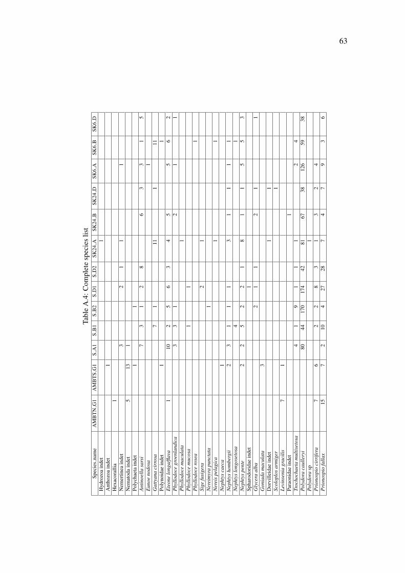
63
Tabl
eA
.4:C
ompl
ete
spec
ies
list
Spec
ies
nam
eA
MB
TN
G1
AM
BT
SG
1S
A1
SB
1S
B2
SD
1S
D2
SK24
ASK
24B
SK24
DSK
6A
SK6
BSK
6D
Hyd
rozo
ain
det
1A
ntho
zoa
inde
t1
Hex
acor
allia
1N
emer
tinea
inde
t3
21
11
Nem
atod
ain
det
513
1Po
lych
aeta
inde
t1
1A
ntin
oella
sars
i7
31
28
63
31
5E
unoe
nodo
sa1
Gat
tyan
aci
rros
a7
111
111
Poly
noid
aein
det
11
Ete
one
long
a/fla
va1
102
56
34
55
62
Phy
llodo
cegr
oenl
andi
ca3
31
21
1P
hyllo
doce
mac
ulat
a1
Phy
llodo
cem
ucos
a1
1P
hyllo
doce
rose
a1
Sige
fusi
gera
21
Ner
eim
yra
punc
tata
1N
erei
spe
lagi
ca1
1N
epht
ysca
eca
1N
epht
ysho
mbe
rgii
23
11
13
11
11
Nep
htys
long
oset
osa
41
Nep
htys
pent
e2
25
22
18
11
55
3Sp
haro
dori
dae
inde
t1
Gly
cera
alba
21
12
11
Gon
iada
mac
ulat
a3
Dor
ville
idae
inde
t1
1Sc
olop
los
arm
iger
1Le
vins
enia
grac
ilis
71
Para
onid
aein
det
1Tr
ocho
chae
tam
ultis
etos
a4
19
11
12
4Po
lydo
raca
ulle
ryi
8044
170
174
4281
6738
126
5938
Poly
dora
sp1
Pri
onos
pio
cirr
ifera
76
22
83
13
24
Pri
onos
pio
falla
x15
72
104
2728
74
79
36
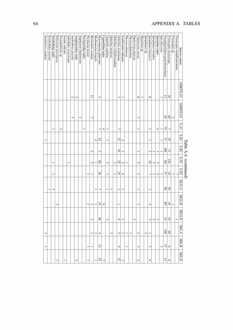
64 APPENDIX A. TABLES
TableA
.4:(continued)Species
name
AM
BT
NG
1A
MB
TS
G1
SA
1S
B1
SB
2S
D1
SD
2SK
24A
SK24
BSK
24D
SK6
ASK
6B
SK6
DP
rionospiom
ultibranchiata7
1P
rionospiosp
31
1P
rionospiosteenstrupi
3840
725
13142
3438
1619
606
8P
seudopolydorapaucibranchiata
1220
7451
10660
5740
8916
14637
14Spio
filicornis1
11
11
2Spionidae
indet4
13
21
Spiophanesbom
byx1
41
2Spiophanes
kroeyeri8
11
210
71
43
13
6Spiophanes
sp2
Magelona
sp1
Chaetozone
setosa8
31
15
21
32
34
Diplocirrus
glaucus1
Pherusa
flabellata1
Pherusa
plumosa
11
1Scalibregm
ainflatum
12
12
41
11
3O
phelinaacum
inata3
722
1625
252
16
59
12O
phelinacylindricaudata
21
Ophelina
modesta
13
Capitella
capitata1
15
11
3C
apitellidaeindet
49
2H
eteromastus
filiformis
47
222
6026
719
484
1352
Mediom
astusfragilis
41
11
21
Myriochele
oculata12
72
21
12
11
Pectinariakoreni
12
11
Pectinariidaeindet
1A
mpharete
lindstroemi
1A
mpharetidae
indet3
2A
nobothrusgracilis
21
Sabellidesoctocirrata
1Sosane
sulcata1
Neoam
phitritesp
2Polycirrus
norvegicus2
1Terebellidae
indet1
11
3Terebellides
stroemi
1Jasm
ineiracaudata
13
1

65
Tabl
eA
.4:(
cont
inue
d)Sp
ecie
sna
me
AM
BT
NG
1A
MB
TS
G1
SA
1S
B1
SB
2S
D1
SD
2SK
24A
SK24
BSK
24D
SK6
ASK
6B
SK6
DSa
belli
dae
inde
t1
1Se
rpul
idae
inde
t1
13
Gas
trop
oda
inde
t4
12
Poly
plac
opho
rain
det
1B
ival
via
inde
t1
23
21
Nuc
ula
cf.s
ulca
ta1
Nuc
ulom
ate
nuis
1Yo
ldie
llaph
ilipp
iana
1M
ytilu
sed
ulis
2C
hlam
ysse
ptem
radi
atus
1C
hlam
yssp
Chl
amys
stri
atum
11
11
1A
nom
iidae
inde
t1
12
7Th
yasi
rasp
22
11
Aca
ntho
card
iaec
hina
ta1
Parv
icar
dium
min
imum
1A
bra
nitid
a5
11
21
Abr
asp
1K
ellie
llaab
yssi
cola
1C
orbu
lagi
bba
28
31
71
Hia
tella
arct
ica
1C
alan
oide
ain
det
103
1C
yclo
poid
eain
det
42
1N
ebal
iabi
pes
1C
umac
eain
det
2E
udor
ella
cf.t
runc
atul
a1
Am
phip
oda
inde
t1
1G
amm
arid
eain
det
13
Lysi
anas
sida
ein
det
2A
mpe
lisca
brev
icor
nis
11
Am
pelis
cacf
.typ
ica
1A
mpe
lisca
mac
roce
phal
a1
1A
mpe
lisca
sp1
Am
pelis
cate
nuic
orni
s2
5C
heir
ocra
tus
sund
ewal
li1
11
1
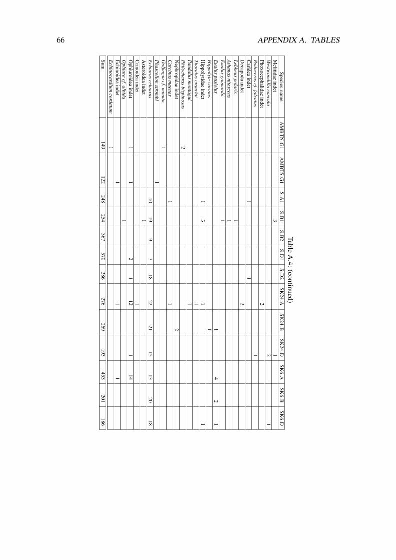
66 APPENDIX A. TABLES
TableA
.4:(continued)Species
name
AM
BT
NG
1A
MB
TS
G1
SA
1S
B1
SB
2S
D1
SD
2SK
24A
SK24
BSK
24D
SK6
ASK
6B
SK6
DM
elitidaeindet
31
Westw
oodillacaecula
21
Phoxocephalidaeindet
2Podocerus
cf.falcatus1
Caridea
indet1
1D
ecapodaindet
2Lebbeus
polaris1
Athanas
nitescens1
Eualus
gaimardii
1E
ualuspusiolus
14
21
Hippolyte
varians1
Hippolytidae
indet1
31
1Thoralus
cranchii1
Pandalusm
ontagui1
Philocheras
bispinosus2
Nephropidae
indet2
Carcinus
maenas
11
Golfingia
cf.minuta
1P
hascolionstrom
bi1
Echiurus
echiurus10
199
718
2221
1513
2018
Asteroidea
indet1
Crinoidea
indet1
Ophiuroidea
indet1
12
112
114
Ophiura
cf.albida1
Echinoidea
indet1
11
Echinocardium
cordatum1
Sum149
122248
254367
570286
276269
193453
201186

67
Table A.5: Feeding mode of each species. The categories No info and Other are placed togetherin the final table. DF = deposit feeders, SDF = subsurface deposit feeders.
Feeding Speciesno info Hydrozoa indetno info Anthozoa indetno info HexacoralliaCarnivore/omnivore Nemertinea indetno info Nematoda indetother Polychaeta indetcarnivore/omnivore (largedetrituslicker) Antinoella sarsiCarnivore/omnivore Eunoe nodosaCarnivore/omnivore(parasite/commensal) Gattyana cirrosano info Polynoidae indetcarnivore/omnivore Eteone longa/flavacarnivore/omnivore Phyllodoce groenlandicacarnivore/omnivore Phyllodoce maculatacarnivore/omnivore Phyllodoce mucosacarnivore/omnivore Phyllodoce roseano info Sige fusigeraother Nereimyra punctatano info Nereis pelagicaScavenger/carnivore/omnivore Nephtys caecaCarnivore/omnivore Nephtys hombergiiCarnivore/omnivore(scavenger) Nephtys longosetosaScavenger/carnivore/omnivore Nephtys penteno info Spharodoridae indetCarnivore/omnivore Glycera albaCarnivore/omnivore Goniada maculatano info Dorvilleidae indetDF Scoloplos armigerDF(SDF) Levinsenia gracilisno info Paraonidae indetsuspension/SDF Trochochaeta multisetosasuspension/SDF Polydora caulleryisuspension/SDF Polydora spSDF(suspension) Prionospio cirriferaSDF(suspension) Prionospio fallaxSDF(suspension) Prionospio multibranchiataSDF(suspension) Prionospio steenstrupiSDF(suspension) Pseudopolydora paucibranchiataSDF Spio filicornisSDF(suspension) Spionidae indetSDF(suspension) Spiophanes bombyxSDF(suspension) Spiophanes kroeyeriSDF(suspension) Spiophanes spSDF(suspension) Magelona spSDF Chaetozone setosaSDF(largesandlicker) Diplocirrus glaucusno info Pherusa flabellataSDF(largesandlicker) Pherusa plumosaDF(suspension) Scalibregma inflatum

68 APPENDIX A. TABLES
Table A.5: (Continued)DF Ophelina acuminataDF Ophelina cylindricaudataDF Ophelina modestaDF Capitella capitataDF Capitellidae indetDF Heteromastus filiformisDF Mediomastus fragilisSDF Myriochele oculataDF(largesandlicker) Pectinaria korenino info Pectinariidae indetSDF Ampharete lindstroemiSDF Ampharetidae indetSDF Anobothrus gracilisSDF Sabellides octocirrataSDF Sosane sulcatano info Neoamphitrite spSDF(dissolvedmatter/symbionts) Polycirrus norvegicusSDF Terebellidae indetSDF Terebellides stroemiSuspension(SDF) Jasmineira caudataSuspension Sabellidae indetno info Serpulidae indetno info Gastropoda indetno info Polyplacophora indetno info Bivalvia indetDF Nucula cf. sulcataDF Nuculoma tenuisno info Yoldiella philippianano info Mytilus edulisno info Chlamys septemradiatusno info Chlamys spno info Chlamys striatumno info Anomiidae indetDF Thyasira spsuspension Acanthocardia echinatasuspension Parvicardium minimumsuspension/SDF Abra nitidaother Abra spno info Kelliella abyssicolasupension Corbula gibbano info Hiatella arcticano info Nebalia bipesno info Cumacea indetno info Eudorella cf. truncatulano info Amphipoda indetno info Gammaridea indetno info Lysianassidae indetsuspension Ampelisca brevicornissuspension Ampelisca cf. typicasupension Ampelisca macrocephala
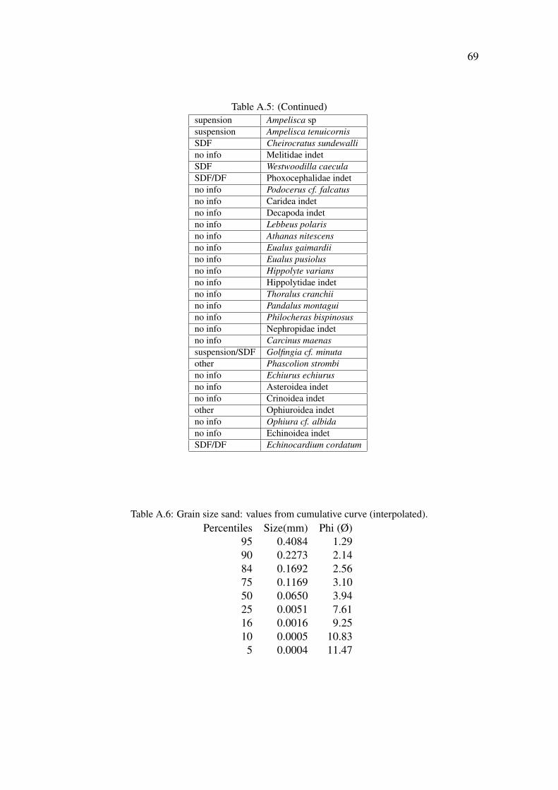
69
Table A.5: (Continued)supension Ampelisca spsuspension Ampelisca tenuicornisSDF Cheirocratus sundewallino info Melitidae indetSDF Westwoodilla caeculaSDF/DF Phoxocephalidae indetno info Podocerus cf. falcatusno info Caridea indetno info Decapoda indetno info Lebbeus polarisno info Athanas nitescensno info Eualus gaimardiino info Eualus pusiolusno info Hippolyte variansno info Hippolytidae indetno info Thoralus cranchiino info Pandalus montaguino info Philocheras bispinosusno info Nephropidae indetno info Carcinus maenassuspension/SDF Golfingia cf. minutaother Phascolion strombino info Echiurus echiurusno info Asteroidea indetno info Crinoidea indetother Ophiuroidea indetno info Ophiura cf. albidano info Echinoidea indetSDF/DF Echinocardium cordatum
Table A.6: Grain size sand: values from cumulative curve (interpolated).Percentiles Size(mm) Phi (Ø)
95 0.4084 1.2990 0.2273 2.1484 0.1692 2.5675 0.1169 3.1050 0.0650 3.9425 0.0051 7.6116 0.0016 9.2510 0.0005 10.835 0.0004 11.47
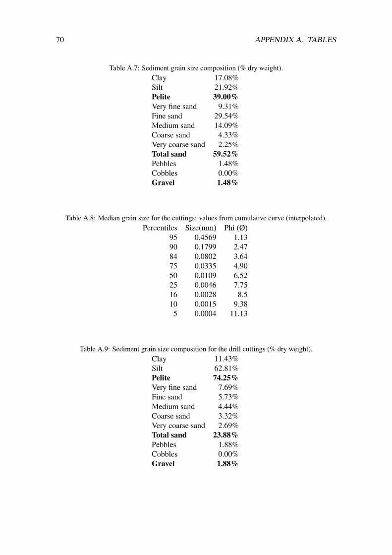
70 APPENDIX A. TABLES
Table A.7: Sediment grain size composition (% dry weight).Clay 17.08%Silt 21.92%Pelite 39.00%Very fine sand 9.31%Fine sand 29.54%Medium sand 14.09%Coarse sand 4.33%Very coarse sand 2.25%Total sand 59.52%Pebbles 1.48%Cobbles 0.00%Gravel 1.48%
Table A.8: Median grain size for the cuttings: values from cumulative curve (interpolated).Percentiles Size(mm) Phi (Ø)
95 0.4569 1.1390 0.1799 2.4784 0.0802 3.6475 0.0335 4.9050 0.0109 6.5225 0.0046 7.7516 0.0028 8.510 0.0015 9.385 0.0004 11.13
Table A.9: Sediment grain size composition for the drill cuttings (% dry weight).Clay 11.43%Silt 62.81%Pelite 74.25%Very fine sand 7.69%Fine sand 5.73%Medium sand 4.44%Coarse sand 3.32%Very coarse sand 2.69%Total sand 23.88%Pebbles 1.88%Cobbles 0.00%Gravel 1.88%

71
Table A.10: Median grain size for the fine sediment: values from cumulative curve (interpolated).Percentiles Size(mm) Phi (Ø)
95 0.1551 2.6990 0.1111 3.1784 0.0915 3.4575 0.0684 3.8750 0.0088 6.8225 0.0009 10.1116 0.0005 11.1110 0.0004 11.445 0.0003 11.72
Table A.11: Sediment grain size composition for the fine sediment (% dry weight).Clay 33.11%Silt 23.97%Pelite 57.08%Very fine sand 15.12%Fine sand 21.46%Medium sand 4.31%Coarse sand 1.55%Very coarse sand 0.48%Total sand 42.92%Pebbles 0.00%Cobbles 0.00%Gravel 0.00%

72 APPENDIX A. TABLES

Appendix B
Figures
Transform: Fourth root
Resemblance: S17 Bray Curtis similarity
Treatment
Control
24mm
6mm
2D Stress: 0.17
Figure B.1: Multi Dimensional Scaling (MDS) based on fourth root faunal counts, as a func-tion of treatment without the two most abundant species, Polydora caulleryi and Pseudopolydorapausibranchiata.
73

74 APPENDIX B. FIGURES
Transform: Fourth root
Resemblance: S17 Bray Curtis similarity
AMBTN_G1AMBTS_G1S_A16
S_B16S_B2S_D16S_D2SK24_A14SK24_B14SK24_D14SK6_A13SK6_B13SK6_D13
2D Stress: 0.01
Figure B.2: Multi Dimensional Scaling (MDS) based on fourth root faunal counts, of the 11experimental boxes and the ambient grab samples.
Transform: Fourth root
Resemblance: S17 Bray Curtis similarity
Frame
A
B
D
2D Stress: 0.17
Figure B.3: Multi dimensional scaling (MDS) based on fourth root faunal counts, of the 11 exper-imental boxes, leaving out the two ambient grab samples, as a function of frame, without the twomost abundant species, Polydora caulleryi and Pseudopolydora Pausibranchiata.
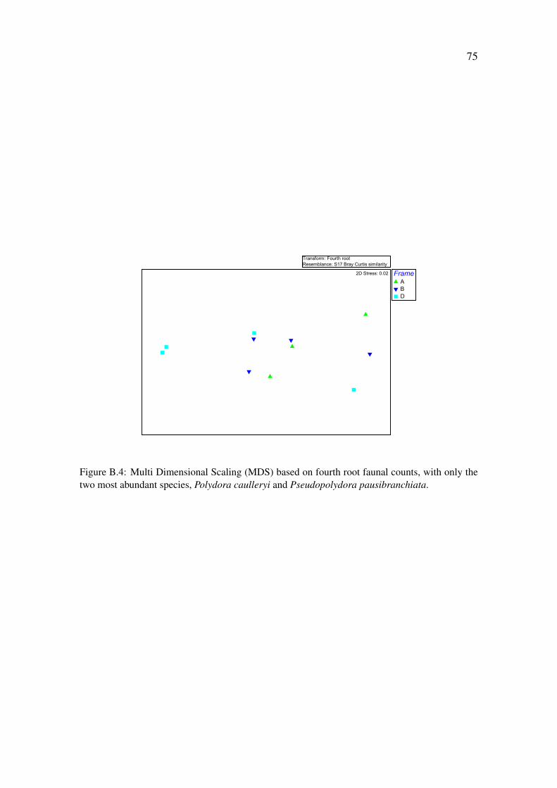
75
Transform: Fourth root
Resemblance: S17 Bray Curtis similarity
Frame
A
B
D
2D Stress: 0.02
Figure B.4: Multi Dimensional Scaling (MDS) based on fourth root faunal counts, with only thetwo most abundant species, Polydora caulleryi and Pseudopolydora pausibranchiata.


![API - The Flow Propierties of Drilling Muds[1]](https://img.pdfslide.us/doc/110x75/563dbbb3550346aa9aaf8103/api-the-flow-propierties-of-drilling-muds1.jpg)


![SPE - Radial Filtration of Drilling Muds[1]](https://img.pdfslide.us/doc/110x75/563dbbb3550346aa9aaf812f/spe-radial-filtration-of-drilling-muds1.jpg)