Effects of the atmospheric phase fluctuation on long-distance measurement

Effects of the atmospheric phase fluctuation on long-distance measurement

Hirokazu Matsumoto and Koichi Tsukahara

Using a phase-locked interferometer, the phase fluctuation of laser beam propagation in the field has beeninvestigated as a function of path length and beam spacing over the wide-frequency range. The higher fre-quency portion of the result shows good agreement with the result reported by Clifford. The variance of theaveraged data follows a -1/3 power law for the theoretical averaging time in the homogeneous field. Usingthese data, the effect of the phase fluctuation is analyzed on practical long-distance measurements by a two-color method.

1. Introduction

Precise measurement of ground deformation is re-quired in the fields of earth science and more practicallyearthquake prediction. Recently, to measure very smallhorizontal changes of the ground, a multiwavelengthelectromagnetic distance measuring systeml4 was de-veloped, which uses two different wavelength lasers andone microwave to correct for the velocity of light af-fected by the atmospheric air condition. This ap-plication, however, is still limited by turbulence, scat-tering, and attenuation of the wave propagating in theatmospheric air. Above all, the fluctuations of intensityand phase caused by the turbulence become seriouswhen high-accuracy measurement is required.5

Many experimental as well as theoretical studies havealready been made concerning the fluctuations of theintensity and phase of the propagating wave. The re-sults, however, have not always been in good agreement.Moreover, quantitative data on turbulence in the lowerfrequency region, which are important in deciding theoptimum measuring time in precise distance measure-ment in the field, are still scarce.

This paper presents experimental results on thephase fluctuation of the propagating wave, particularlyin the low-frequency range, and discusses the effects ofphase fluctuations on long-distance measurement.

II. Theoretical Considerations

According to Tatarski6 and to Clifford et al.,7,8 thestructure function of the phase s of the plane light wavepropagating in a locally homogeneous field is ex-pressed:

D(p) = (k(r + p)-(r)]2)av= 2.9lk 2 LCn2p 5

/3, NJXT g < Lo, (1)

where k is the wave number of the propagating wave,L the length between emitting and receiving positions,Cn2 the structure parameter of turbulence, p the spac-ing between two observing points on the surface of thereceiving point, and Lo the maximum scale of turbu-lence.

The spectrum of the autocorrelation function W,,(f)was obtained by Clifford to be

WW ={ O.033k2

LCn 2v

5/3

[ - cos(27rpf/v)]f-/ 3, p << vX,

10.066k 2LCn 2v 5/3[ - cos(27rpf/v)]f- 8 /3 , p >> AXE.

(2)

The time-lag autocorrelation function of the differ-ence between the phases at the two points separated bya distance of p is defined:

RO(T) = ([o(rt) - (r + p,t)][0(r,t + T)

- k(r + p,t + )])av= 2B(Vr) - Bo(p - vr) - Bo(p + VT) [Bo(-) - 0],

(3)

Hirokazu Matsumoto is with National Research Laboratory ofMetrology, 1-1-4 Umezono, Sakura-mura, Niihari-gun, Ibaraki 305,Japan, and K. Tsukahara is with Geographical Survey Institute, 1Kitazato, Yatabe-machi, Tsukuba-gun, Ibaraki 305, Japan.

Received 12 December 1983.0003-6935/84/193388-07$02.00/0.© 1984 Optical Society of America.

Bo(wr) = ((r,t) - (r -VTt))aV

= 2 7r f F(K,O)KdK Jo(xvr),

F(K,O) = 0.033irCn 2k 2L[1 + k sin(K 2 L/k)/(x 2 L)]' 1 1/3

(4)

(K < Km),

(5)

where v is the wind velocity perpendicular to the wavepath, Bq(v-r) the spatial phase covariance function, andKm - 27r/lo (lo is the smallest size of turbulence).

3388 APPLIED OPTICS / Vol. 23, No. 19 / 1 October 1984

Next, we consider the variance of the averagedphase-fluctuation values. For an averaging number(time) of N(T), the variance of the averaged values isexpressed by the covariance:

1 N-1N-1varJxNJ = - cov(xixj)

N 2 i=O j=O x,0

=varix + - cov(x0 ,X i). (6)N N(6According to the nature of the autocovariance function,we can get

var[xT} = 2 ( --T Rx(r)dr, (7)

where Rx () is the autocorrelation function of time-lagT. Substituting Eqs. (1) and (3)-(5) into Eq. (7), weobtain explicitly that

varlYNI 47r2(0.033)Cn 2 k2 L r a I k sK2L

T JO +K2L k

G f (i - [2JO(KVr) -JO(KP-KVT)

-JO(Kp + KVr)]d-r. (8)

In this equation, G is calculated as follows:

1 X 2-2rG = ZF (-1)r 22r (V)2+(KV)2 T r (r!)(2r + 1)(2r + 2) [2(,vT)sr+S

- (KP - KvT)2r+2 - (KP + KvT)2r+2 + 2(KP)2r+2]. (9)

For lo << vT << p, we obtain G -T* JO(Kp). We thusfind that

var[xTI 2.91Cn2 k2 Lp 5 /3 . (10)

As easily known from Eq. (10), the variance of the av-eraged values does not depend on the averaging timeT.

Next, when vT is far larger than p, we obtain

G _P2 JO(KvT), (11)

2.91Cn 2 k2 Lp 2 (p < vT LO). (12)va~xT, t (vT)113

As a result, varIT1 decreases slowly with averaging timeT according to the -1/3 law.

When vT exceeds the maximum scale of the turbu-lence Lo, the field cannot be considered homogeneousand isotropic, so we cannot define Eq. (3). Then,varlxT) is considered inversely proportional to the av-eraging time.

111. Experiment

A. Principle

The phase fluctuation of the atmospheric air has beenmeasured using various types of interferometer, mainlyfringe-counting interferometers whose resolutions aregenerally not high. For measuring the phase fluctua-tion with high resolution, a phase-locked interferometeris adopted. The output intensity I from a two-beaminterferometer is simply described by

I = + I2 + 2V7Icoso,

0 = 27rn(Ll -L2)/, (13)

where I, and I2 are the intensity of the two beams, n isthe refractive index of air, L1 and L2 (L1 - L2) are thegeometrical path lengths and X is the vacuum wave-length of the light source. If we detect both I, and I2separately and subtract them from I, we obtain 2V/IIcoso. The value of 2v'7i71 cosk is not affected by thechanges of I, and I2 as far as 0 = r/2 + 2mir (m is aninteger). First, the voltage applied to a piezoelectrictransducer (PZT) is adjusted so that the phase of thefringe may be 7r/2 + 2m7r. If the refractive index of airalong L1 is changed compared with that along L2, thephase of the interference fringe varies and, accordingly,the intensity of the detected signal varies. The voltageapplied to the PZT decreases with the intensity varia-tion, and L2 becomes short so that the phase of thesignal may return to the original one and the opticalpath length is kept constant. Therefore, the change ofthe refractive index is substituted for the change of thepath length, namely, the change of the appliedvoltage.

B. Experimental Setup

The interferometer developed is comprised of somesimple components containing the PZT with a planemirror as shown in Fig. 1. A 0.63-,m He-Ne laser beamis expanded and collimated by lenses and goes to a re-flecting plane mirror Q which is placed far away fromthe light source. The beam reflected from the mirrorreturns to the position near the light source and is splitinto two thin beams through a screen plate having twosmall (2-mm diam) holes separated by a distance of p.The positions of the hole H and the PZT are moved toalter p. One beam goes to a beam splitter 1 directly andthe other goes to it after reflecting at the PZT forforming interference fringes. The resulting interfer-ence fringe is detected by photodetector A, while thebeams reflected at beam splitter 2 are detected byphotodetectors B and C. These detected signals areinput to a differential amplifier through operationalamplifiers, so that the effect of the intensity change dueto atmospheric turbulence can be canceled. The signalis filtered by a low-pass filter whose cutoff frequency is-300 Hz and is applied to the PZT through a high-voltage amplifier so that the variation of the path lengthdue to phase fluctuation is compensated. The variationis recorded on a chart recorder and also is input to aHewlett-Packard spectrum analyzer. The high-fre-quency spectrum of the variation is studied using theanalyzer; the low-frequency spectrum and the varianceof the means are analyzed from data read out from thechart using a computer. The experimental error isseveral percent of the measured voltage.C. Experimental Conditions

Measurements of phase fluctuation were madechoosing six clear days in July and August of 1983. Theconditions at the time of the experiments were 20°Ctemperature and -1-m/sec wind velocity. Most of ourexperiments were carried out from 11 p.m. to 3 a.m., 3-6

1 October 1984 / Vol. 23, No. 19 / APPLIED OPTICS 3389

Bench

Reflecting Mirrors IDeptector R1 ,. - .. I

E

I eI_I

Reflecting Mirror

Stand

Chart RecorderandSpectrum Analyzer

Amplifier AmplifierFig. 1. Schematic diagram of the experimental setup.

S ~ ~ ~

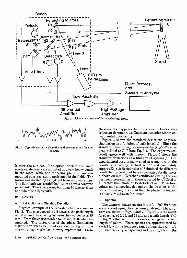
Fig. 2. Typical chart of the phase fluctuation recorded as a functionof time.

h after the sun set. The optical devices and someelectrical devices were mounted on a very heavy benchin the room, while the reflecting plane mirror wasmounted on a steel stand positioned in the field. Themirror was isolated by a vinyl tent from wind vibrations.The light path was established 1.1 m above a concretepavement. There were some buildings 10 m away fromone side of the light path.

IV. Results

A. Distribution and Standard Deviation

A typical example of the recorded chart is shown inFig. 2. The chart speed is 1.5 cm/sec, the path lengthis 100 m, and the spacing between the two beams is 75mm. From the chart recorded for 80 sec, 1200 data weresampled. The histograms of the phase-fluctuationdistribution were calculated as shown in Fig. 3. Thedistributions are similar in every experiment. From

these results it appears that the phase-fluctuation dis-tribution demonstrates Gaussian statistics within ex-perimental uncertainty.

Figure 4 shows the standard deviations of phasefluctuation as a function of path length L. Since thestandard deviation o-, is expressed by (Dk/2) 1 /2 , o isproportional to L1/2 from Eq. (1). The experimentalresult agrees well with theory. Figure 5 shows thestandard deviations as a function of spacing p. Ourexperimental results show good agreement with theresults obtained by Clifford et al.

7 and completelysupport Eq. (1); Bertolotti et al.9 obtained the differentresult that s,/, could not be approximated for distancesp above 30 mm. Weather conditions during the ex-periment were similar to those reported by Clifford etal. rather than those of Bertolotti et al. Therefore,values may somewhat depend on the weather condi-tions. However, it is noted that the phase fluctuationis not saturated even for large p.

B. Spectra

The temporal power spectra in the 0.1-300-Hz rangeare analyzed using the spectrum analyzer. These re-sults are shown in Figs. 6 and 7. Figure 6 is the resultfor spacings of 5, 25, and 75 mm and a path length of 40m; Fig. 7 is the result for the same spacings and a pathlength of 150 m. These spectra are approximated bya -2/3 law in the frequency range of less than fo = v/p(v: wind velocity, p: spacing) and by a -8/3 law in the


\ ~~~~~~~~~~~~~~~~~~~~~~I

20'

1

( A) (B)

20G

loC

0-l 80° 0 180°

200

100

0-180o

(C)

1800

(D)

Fig. 3. Histograms of the phase fluctuations obtained for a spacing of 25 mm and path lengths of (A) 20 m, (B) 40 m, (C) 100 m,and (D) 150 m.

300F-

100 - I I I I ' ' ' ' I I

50

40-

30

20 - o July 28

x July 24

10 I I I I ' ' ' ' I I10 20 30 40 50

L (m)

2001-

a,

,1 00

5040

30

20-

100 150 200 0.5 1 2p (cm)

3 4 5 7 10

Fig. 4. Standard deviations o- of the phase fluctuations for a spacingof 25 mm as a function of path length.

Fig. 5. Standard deviations v h of the phase fluctuations for pathlengths of 40, 100, and 150 m as a function of spacing.


6 =73.50

~~~~~~~~~~~~~~~~~~~~~~~I

0Da,7U

I I 1 I1 I I I I I I IIl

0 60ocf'/x

L=150mL=100m

1/I x L= 40m

i I, I I II I I I I , , ,,1

I

6 = 54.4!

I A I I -

. . . . . . . .

uvu_400_

.I

100 10000.1 1 10f ( Hz)

Fig. 6. Temporal power spectra of the phase fluctuations WO(f) fora path length of 40 m and spacings of 5, 25, and 75 mm.

11

100

I01

iol

10-E

0.1 1 10f ( Hz)

frequency range above fo. Good agreement betweenthis result and the theory of Clifford8 was obtained. Itis noted that Clifford's theory holds for various pathlengths.

The behavior of the spectrum at low frequency is ofconsiderable practical interest because it is useful fordeciding the measuring time in practical uses such asdistance measurement. These phase fluctuations arerecorded on a chart recorder for 10 min and are read outevery 0.5 sec. The temporal power spectra are shownin Fig. 8. The path length is 100 m and the spacings are25 and 75 mm. It is likely that the power spectrum goesout of the -2/3 law as the frequency decreases, com-pared with a frequency of 0.05 Hz. This frequency maybe estimated from the wind velocity divided by theouter scale whose value is found to be a few meters inthis experiment.

io-'I-

10-2k

1- 3H

10-4

0.001 0.01 0.1 1

f (Hz)

Fig. 8. Temporal power spectra Wk(f) in the low-frequency rangefor a path length of 100 m and spacings of 25 and 75 mm.

c

._

-ni-

1001-

10

100 100010 100

Averaging Time ( sec)

Fig. 7. Temporal power spectra of the phase fluctuations WO(f) fora path length of 100 m and spacings of 5, 25, and 75 mm.

Fig. 9. Variances of the averaged data as a function of averagingtime. The data are the same as in Fig. 8.


P=75mm L = 150m

0 *00 0 .

25mm 0 0

IV, 005mrn x 'x~

O X

L = lOOm

. P =75mm

.. ....

°o 25mm

us, l

.I1UUU I

,

.

Il

E 0.1

-o

CD

0-0.01

(U

0.001 -

0.1 10

Averaging Time ( s )

Fig. 10. Estimated length variations due to 1as a function of averaging t

Table 1. Standard Deviation (o,,) Obtained Experfor a 50-km Line

150mL (Experiment)

p (mm) 5 25 7a0w () 22 118 32

C., Variance of Averaged Data

A good method for deciding the miexamine the behavior of the standar

l l 0.63-,gm He-Ne and 0.44-Mum He-Cd lasers for a dis-tance of 50 km, assuming the same conditions. Using Eq.(2) we can estimate the standard deviation of the phasefluctuation for the 50-km line as shown in Table I.Using 6X uo(p), we obtain 1080000 as the magnitude ofthe phase fluctuation, which is equvalent to 0.2 mm in

- . length variation. If we hope to measure the 50-km lineA--- -- with a high accuracy of 1 10 , we must constrain the

variation between the distances measured by the two* - laser beams of 0.63 and 0.44 Am within an accuracy of

0.24 mm because the accuracy is -21 times less with thismethod. Therefore, the obtained distance variation of

l l 0.2 mm is marginal.100 1000 It is important to know the averaging time required

to get high accuracy in long-distance measurement. To

the phase fluctuations investigate this, we must estimate the magnitudes of theine. structure parameter Cn2 and the outer scale of the

turbulence, Lo. The structure parameter Cn2 decreaseswith altitude, and according to Walters and Kunkel12Cn2 is proportional to h-4 /3 in daytime and valid up to

rImentally and Estimated a half of the troposphere, where h is the altitude fromthe ground. While it is difficult to estimate the outer

50 km scale Lo, according to Tatarski6 Lo is proportional to(Estimation) altitude, namely, Lo = Kh (K - 0.4) and tens to hundreds

'5 300 of meters in the troposphere.5 18000 Figure 10 shows the length variation caused by at-

mospheric turbulence as a function of averaging time.This is obtained by using the experimental data and theformulas of Cn2 c h-4 /3 and Lo h which may be validup to hundreds of meters in altitude. From this figureit is evident that averaging times of more than several

easuring time is to tens of seconds are required to obtain an accuracy ofI deviations of the better than 0.1 mm.

averaged data obtained with various averaging times.Using the chart mentioned in the previous section, theaveraged values are obtained for each 0.5 sec. Figure9 is the variance of the averaged values as a function ofaveraging time. It can be concluded that in the shortaveraging time range, at first the variance decreasesaccording to a -1/3 law with averaging time, and as theaveraging time increases, the variance decreases ac-cording to a -1 law. This is in good agreement with thetheoretical result derived earlier.

V. Analysis of Errors Affecting DistanceMeasurement

We now estimate the magnitude of the phase fluc-tuation between the laser beams of two wavelengths atthe receiving point after they propagate over a longdistance of 50 km. The two beam paths are separatedby the dispersion of air and the spacing depends on themagnitude of the dispersion. According to Thayer,10the maximum spacing is pmax = L 2(dnl/dz - dn2/dz)/8,assuming that the refractive-index gradient is constant.Here L is the path length, dnl/dz and dn2/dz are thegradients of the refractive indices for different wave-lengths, and the mean value is given by 2 pma/3. Bergand Carter" investigated the path spacing of lightbeams by analyzing the actual refractive-index gradientdata obtained in Hawaii. According to Berg and Carter,the mean path spacing is expected to be 30 cm for the

VI. Conclusions

The formula for phase fluctuation derived by Cliffordwas experimentally shown to be valid for path lengthsup to 150 m and for spatial spacings up to 75 mm. Thepower spectrum of the phase fluctuation goes downapart from a -2/3 law as the frequency decreases overthe frequency fo of (wind velocity)/(outer scale). Thevariance of the averaging data decreases according toa -1/3 law with averaging time up to 1/fo. Assumingthat the structure function formula is still valid for longdistances, an averaging time of several tens of secondsis adequate to obtain a high (10-7) accuracy in 50-kmline measurements using a two-color method.

This work was supported in part by the U.S. Geo-logical Survey and by the National Bureau of Standards.The authors appreciate the hospitality of the Joint In-stitute for Laboratory Astrophysics, where K. T. was avisitor during part of this work and where H. M. isworking at the present time, and they thank JudahLevine and John A. Magyar for discussions and sug-gestions.


_; ,-- h-- im-

l0in

I

lI

1

References

1. P. L. Bender and J. C. Ownes, "Correction of Optical DistanceMeasurements for the Fluctuating Atmospheric Index of Re-fraction," J. Geophys. Res. 70, 2461 (1965).

2. J. C. Owens, Invited paper presented to the International Asso-ciation of Geodesy and Geophysics, 25 Sept.-7 Oct. 1967, Lucerne,Switzerland.

3. E. N. Hernandez and K. B. Earnshaw, "Field Tests of a Two-Laser (4416 A and 6328 A) Optical Distance-Measuring Instru-ment Correcting for the Atmospheric Index of Refraction," J.Geophys. Res. 77, 6994 (1972).

4. L. E. Slater and G. R. Huggett, "A multiwavelength Distance-Measuring Instrument for Geophysical Experiments," J. Geo-phys. Res. 81, 6299 (1976).

5. J. Levine, "Electromagnetic Distance Measurements," JILAReport (1978).

6. V. I. Tatarski, Wave Propagation in a Turbulent Medium(McGraw-Hill, New York, 1961).

7. S. F. Clifford, G. M. B. Bouricius, G. R. Ochs, and M. H. Ackley,"Phase Variations in Atmospheric Optical Propagation," J. Opt.Soc. Am. 61, 1279 (1971).

8. S. F. Clifford, "Temporal-Frequency Spectra for a Spherical WavePropagating through Atmospheric Turbulence," J. Opt. Soc. Am.61, 1285 (1971).

9. M. Bertolotti, M. Carnevale, L. Muzii, and D. Sette, "Interfero-metric Study of Phase Fluctuations of a Laser Beam Through theTurbulent Atmosphere," Appl. Opt. 7, 2246 (1968).

10. G. D. Thayer, ESSA Technical Report IER56-ITSA53 (1967).11. E. Berg and J. A. Carter, "Distance Corrections for Single- and

Dual-Color Lasers by Ray Tracing," J. Geophys. Res. 85, 6513(1980).

12. D. L. Walters and K. E. Kunkel, "Atmospheric ModulationTransfer Function for Desert and Mountain Locations: the At-mospheric Effects on r," J. Opt. Soc. Am. 71, 397 (1981).

Meetings Calendar continued from page 3387

1985August

18-23 29th Ann. Int. Tech. Symp. on Optical & Electro-OpticalEng., San Diego SPIE, P.O. Box 10, Bellingham,Wash. 98227

October

4-9 Lesson of the Quantum Theory, Niels Bohr Inst. AIPBohr Library, 335 E. 45th St., New York, N.Y.10017

15-18 OSA Ann. Mtg., Wash., D.C. OSA Mtgs. Dept., 1816Jefferson P., N. W., Wash., D.C. 20036

November

11-14 4th Int. Congr. on Applications of Lasers & Electro-Optics, San Francisco Laser Inst. of Am., 5151 Mon-roe St., Suite 118W, Toledo, Ohio 43623

December

8-13 10th Ann. Int. Conf. on Infrared & Millimeter Waves,Lake Buena Vista, Fla. K. Button, MITNatl. MagnetLab., Bldg. NW14, Cambridge, Mass. 02139

1986January

19-24 Optical & Electro-Optical Eng. Symp., Los AngelesSPIE, P.O. Box 10, Bellingham, Wash. 98227

February

9-15 Astronomical Instrumentation Conf., Tucson SPIE,P.O. Box 10, Bellingham, Wash. 98227

13-14 Optical Fiber Sensors, OSA Top. Mtg., San DiegoOSA Mtgs. Dept., 1816 Jefferson P., N.W., Wash.,D.C. 20036

March

9-14 Mcrolithography Conf., Santa Clara SP1E, P.O. Box 10,Bellingham, Wash. 98227

June

9-13 Quantum Electronics Int. Conf., Phoenix OSA Mtgs.Dept., 1816 Jefferson P., N.W., Wash., D.C. 20036

10-13 Conf. on Lasers & Electro-Optics (CLEO '86), SanFrancisco OSA Mtgs. Dept., 1816 Jefferson PI., N.W.,Wash., D.C. 20036

August

September

? Gradient-Index Optical Imaging Systems (Grin VI), ItalyD. Moore, Inst. Optics, U. Rochester, Rochester, N. Y.14627

9-22 Niels Bohr Memorial Exhibition, Copenhagen Town HallAIP Bohr Library, 335 E. 45th St., New York, N.Y.10017

15-20 Optical & Electro-Optical Eng. Symp., CambridgeSPIE, P.O. Box 10, Bellingham, Wash. 98227

17-19 Mathematics in Signal Processing Conf., Bath TheDeputy Secretary, Inst. of Mathematics & Its Appli-cations, Maitland House, Warrior Square, South-end-on-Sea, Essex SS1 2JY, England

22-25 Picture Archiving & Communications Systems forMedical Applications Mtg., Kansas City SPIE, P.O.Box 10, Bellingham, Wash. 98227

17-22 30th Ann. Int. Symp. on Optical & Electro-Optical Eng.,San Diego SPIE, P.O. Box 10, Bellingham, Wash.98227

14-19 Optical & Electro-Optical Engineering Symp., CambridgeSPIE, P.O. Box 10, Bellingham, Wash. 98227

October

5-10 Optical & Electro-Optical Eng. Symp., CambridgeSPIE, P.O. Box 10, Bellingham, Wash. 98227

21-24 OSA Ann. Mtg., Los Angeles OSA Mtgs. Dept., 1816Jefferson P., N. W., Wash., D.C. 20036

November

10-13 5th Int. Congr. on Applications of Lasers & Electro-Optics, Boston H. Lee, Laser Inst. of Am., 5151Monroe St., Suite 118W, Toledo, Ohio 43623


Documents

Effects of the atmospheric phase fluctuation on long-distance measurement