Effects of Rules of Origin on FTA Utilization

Rates and Country Welfare

Nan Xu∗

This Draft: August 2016

Abstract

Free trade agreements are generally under-utilized. Assuming full utilization overstates the

benefits and overlooks the substantial distortions generated by free trade preferences. This

paper investigates the impacts of rules of origin on FTA utilization rates and on country welfare

in the context in which there is a vertical production linkage between FTA members. I develop

a general equilibrium model featuring the variable and fixed costs of complying with ROOs. A

binding ROO forces exporters to employ more locally produced inputs instead of using the most

efficient manufacturing process. Additionally, firms face fixed documentation costs due to the

administrative process of obtaining certificates of origin. Whether firms utilize an FTA depends

on the tariff benefits net of the extra costs. Both local analytical solutions and global numerical

results show that: (1) as the ROO becomes stricter, the FTA utilization rate decreases and the

dominant extensive margin drives down the wage rate in the downstream country; (2) a slightly

binding ROO encourages regional production, and the welfare effects of ROOs are ambiguous

depending on the elasticity of substitution between varieties.

Keywords: free trade agreement, rules of origin, general equilibrium, welfare effectJEL Classification: C63, F12, F13, F16

∗Department of Economics, University of Colorado at Boulder, 256 UCB, Boulder, CO 80309-0256. Email:nan.xu@colorado.edu

1 Introduction

Free Trade Agreements (FTAs) are one of the most popular forms of trade liberalization in the past

10 years. The World Trade Organization records more than 200 active regional trade agreements

by January 2012. FTAs are designed to promote bilateral trade between participating countries

by reducing tariffs and other trade barriers. The entry into these agreements is expected to be

beneficial for exporters, since preferential market access can help firms export more and earn more

profits. Most analyses so far on the impacts of FTAs assume that these agreements are used by all

exporters. However, recent statistics reveal that the average FTA utilization rate is far below 100

percent, meaning that only a proportion of exporters actually take advantage of FTA preferences.

Why are many exporting firms unwilling to engage in the FTA framework? What are the actual

effects of FTAs on bilateral trade and country welfare?

This paper documents three stylized facts on FTA utilization and the associated costs generated

by rules of origin, which motivates a re-examination of FTA welfare effects in the context of partial

utilization. First, the utilization rates of FTAs are low in general. Most trade within an FTA

region takes place under the MFN tariff rates, rather than under the preferential tariff rates.

For instance, the US Generalized System of Preference (GSP) provides duty-free market access

to developing countries, but 40 percent of imports qualifying for GSP entered the US market

without claiming the tariff benefits in 2008 Similarly, even though the ASEAN-Korea FTA permits

5 percent tariff reduction, only one fifth of Korean exporters utilize the preference (Cheong and

Cho, 2009). This suggests that assuming full utilization would overestimate the benefits of FTAs

on economic outcomes. Second, strict rules of origin could be a reason for low FTA utilization

rates, as it prevents goods that contain high non-regional value content from being eligible for

preferential tariffs, especially in regions where countries have close vertical linkages in production

with FTA outside countries. The methods of origin determination vary across products and across

FTAs, which further complicates the use of FTA preferences. Third, administrative compliance

and documentation costs offset tariff margin attractiveness. Rules of origin are often expensive to

document. Exporters must obtain a certificate of origin from its national government and present it

to the customs authority of the importing government. Herin (1986) shows that the cost of proving

origin leads over a quarter of European FTA exports to pay the MFN tariff, even if the products

satisfy origin. These three facts together suggest the necessity of incorporating the variable and

fixed costs of complying with ROOs into FTA welfare analysis.

In this paper, I develop a general equilibrium model in which utilizing FTA preferences incurs

extra costs and heterogeneous exporting firms endogenously choose whether to be FTA users. ROOs

intend to limit preferences to member parties. Free trade agreements are conditional policies, in

that they require exporters to use at least some level of locally produced inputs. Products are

eligible for zero tariffs only if they are actually produced in the FTA region. Otherwise, the Most

Favored Nation (MFN) tariffs 1 apply. When the ROO is binding, firms have to deviate from their

1MFN tariffs are what countries promise to impose on imports from other members of the WTO, unless the countryis part of a preferential trade agreement (such as a free trade area or customs union). In practice, MFN rates are the

1

optimal production strategies and employ more domestic inputs, which generates additional costs,

in order to meet the ROO criterion. Additionally, to claim the trade preference, exporters must

obtain a certificate from its national government attesting that the good has met the ROO. The

certificate should be presented to the customs authority of the importing government to qualify for

the preferential tariff rate. Going through this administrative procedure incurs additional costs,

called fixed documentation costs. Thus, exporting firms face a tradeoff between enjoying lower

tariffs and paying more variable and fixed costs due to complying with ROOs. Heterogeneous

firms in terms of productivity and intensity of imported inputs would respond differently to the

implementation of FTAs, resulting in the general under-utilization of FTAs.

My model differs from previous studies in that it focuses on the case where there is a vertical

linkage in production between FTA participating countries. This is an interesting case for study

for two reasons. First, ROOs can provide hidden protection for producers of intermediate inputs

within the FTA region. The degree of restrictiveness of the ROO could affect compliance costs and

the value chain in the most fundamental way. The downstream country could source intermediate

inputs worldwide, but turn to import from regional suppliers if the agreement sets a strict rule of

origin. For instance, the trade value of automobile parts and intermediate inputs from the US to

Mexico increases dramatically after the implementation of NAFTA (Oliver et al., 2002). AFTA

also promotes trade in intermediate goods between ASEAN countries (Hiratsuka et al., 2008).

Second, such a production connection between countries is important for welfare analysis, since it

rationalizes welfare gains following a slightly stricter rule of origin. The conventional studies argue

that a stricter rule of origin reduces the FTA utilization rate and mitigates the potential benefits

of the preferential trade arrangement. These conclusions are based on the assumption that the

FTA countries trade horizontally differentiated goods and there is no vertical production linkage

between them. However, as we see in the real world, a large amount of FTAs are signed between

developed and developing countries which are good at different stages of production. In such cases,

ROOs are not always bad. A binding ROO could not only effectively protect regional producers of

intermediate goods from import competition, but also raise country welfare when the elasticity of

substitution between varieties are relatively small.

In order to explore the implications of heterogeneous utilization of a free trade agreement,

I show global numerical solutions to the model by using GAMS. The further decomposition of

welfare effects of ROOs is conducted by local comparative static exercise in the neighborhood of

full utilization. The model yields three main results. First, within an industry, more productive

firms choose to comply with ROOs and utilize the preferential tariffs granted by FTAs, and less

productive firms choose to not comply with ROOs and pay the most favored nation (MFN) tariffs.

This is due to the fact that it is more costly for a firm with a lower productivity to switch to more

expensive intermediate inputs produced locally, and the firm, as a result, is less likely to comply

with the rule and claim preferential tariffs. Also, an industry that heavily relies on imported inputs

tends to have a low FTA utilization rate if the agreement sets a small tariff margin, a strict ROO,

highest (most restrictive) that WTO members charge one another.

2

and complicated documentation procedures.

Second, the intensive use of locally produced inputs due to ROOs generates distortions in the

labor market. As ROOs become stricter, there are two opposing factors that influences labor

demand. On the extensive margin, the trade preferences will be utilized by fewer exporters. For

those who exported under preferential tariffs before, an exit from the FTA framework leads to a

reduction in the demand for local inputs, since they no longer need to comply with the origin rule.

On the intensive margin, for those who are still using FTA, more domestic inputs are demanded due

to the tightening local content requirement. The overall effect on wage depends on the distribution

of sales of FTA users and nonusers. The local comparative static analysis and the numerical

results show that the extensive margin dominates. The total demand for labor decreases in the

restrictiveness of ROOs. So does the equilibrium wage rate.

Third, regarding the welfare effects of ROOs on FTA participating countries, the elasticity

of substitution between varieties plays an essential role. The welfare level is measured as real

income. The overall effects of ROOs on country welfare can be decomposed into three channels.

One is income channel, in that a stricter ROO generates large distortions in manufacturing process

and forces more exporters to be FTA non-users and pay the MFN tariffs. Thus, the importing

country earns more tariff revenues. Also, labor income changes with ROOs in a general equilibrium

framework. The second channel is through terms of trade. The exporting prices charged by the

firms which are affected ROOs are jointly determined by the restrictiveness of ROOs, domestic

labor cost, and the MFN tariff rates. Higher individual prices benefit the exporting country but

hurt the importing country. The last one is variety channel. The price index of differentiated

varieties decreases with the number of varieties available in the market. Thus, firm entry raises

country welfare. The magnitude of the variety effect depends on how substitutable the varieties

are.

The overall effects of ROOs on country welfare are considered in two seperate cases. If the

elasticity of substitution between varieties is relatively small, both FTA participating countries

experience welfare increase, which is mainly driven by the significant positive variety effect. In such

a case, consumers benefit more from the introduction of new varieties. Resources are allocated to

the more efficient producers and a tighter ROO induces the production of intermediate goods to

move from the outside country to within the FTA area. ROOs help protect regional producers and

promote regional trade in intermediate and final goods. If the elasticity of substitution is relatively

large, the welfare of the upstream country, which is more efficient in producing intermediate inputs,

develops an inverted-U shape relationship with ROOs. When the ROO is slightly binding, the

positive income effect and variety effect outweigh the negative price effect, and as a result, country

welfare increases with ROOs. As the ROO rises further, the distortions in firm production generated

by a strict ROO have a larger impact on product prices and the negative price effect (terms of trade)

is a more important determinant of welfare, implying a decrease of welfare with ROOs. The welfare

of the downstream country declines following a stricter ROO, since variety effect is negatively

correlated to the elasticity of substitution between varieties and the negative terms of trade effect

3

dominates. Both local analytical solutions and simulation results confirm these conclusions.

There is usually a hot debate over a suitable rule of origin for each industry before a free

trade agreement is signed. The underlying policy goal of setting ROO is to protect domestic

producers and improve returns to local factors of production. But the actual effects of origin rules

are not well understood. Demidova et al. (2006) and Ju and Krishna (2005) incorporate binding

ROOs which allow firms to escape paying tariffs but involve an additional per-unit cost in order

to satisfy local content requirements. They examine the impacts of FTA on wage in a general

equilibrium framework, and conclude that stricter ROOs reduce the wage while raising the cutoff

for firms invoking ROOs. But their work does not take into account domestic input producers

whom ROOs primarily aim to protect. There is also no attention given to the magnitudes of the

increase in unit cost caused by rules of origin. The other type of extra costs that may prevent

exporters from utilizing FTA preferences is fixed documentation costs. In the literature, Brenton

and Manchin (2003) points out that FTAs are not fully exploited because of the costs of proving

origin and difficulties in passing though customs. A simpler and less demanding system would

make it easier for small companies in developing countries to obtain preferential access to foreign

markets. Cherkashin et al. (2009) argue that firm heterogeneity and higher fixed costs of exporting

due to using FTAs can rationalize partial utilization. But this strand of literature does not consider

firms’ responses to local content requirements in order to be qualified for trade preferences. Neither

the additional variable costs nor fixed costs accompanied with FTAs are negligible in the analysis

of firms’ decisions on the use of FTAs.

The rest of the paper is organized as follows. Section 2 documents three stylized facts on FTA

utilizations and Rules of Origin. In section 3, I derive a partial equilibrium to analyze firms’ decision

on the use of conditional trade preferences and investigate the determinants of FTA utilization rates.

I then turn to a general equilibrium model to examine the role of ROOs in determining wage rate

and country welfare in Section 4. In section 5, I conduct comparative statics analysis to explore

the local effects of ROOs on FTA utilization and welfare. Section 6 reports the simulation results.

Section 7 concludes.

2 Stylized Facts

2.1 Utilization rates of free trade agreements are low

Free trade agreements are designed to promote regional exports and imports by granting traded

goods preferential or even zero tariff rates. Such tariff margins are obviously beneficial to exporting

firms, and therefore most studies on the effects of FTAs on trade and welfare assume all exporters

in the region are claiming preferential tariffs. However, in fact, the utilization rates of FTAs are far

below 100 percent. Utilization rate is defined as the ratio of value of imports granted under FTA

preference to value of imports eligible for FTA preference. Table 1 lists the actual rates of utilization

of several major FTAs. The utilization rates vary considerably from 5.49% to 71.97%, and most

of them are below 50%. For instance, only 20 percent of Korean firms import goods from ASEAN

4

countries under Korea-ASEAN FTA, and 13.45% of exports from Singapore to China utilize the

preferential tariff rates granted by China-Singapore FTA. NAFTA and China-Pakistan FTA are

relatively intensively utilized and the utilization rates are 55% and 71.79% respectively. But none

of them are close to full utilization. In other words, within an FTA area, only a proportion of

exporting firms choose to export under lower tariffs and there are a large amount of products are

not engaged in the free trade arrangement.

Moreover, FTA utilization rates also vary considerably across industries. Under the US Gener-

alized System of Preference (GSP), the average utilization rate across all industries is 60% in 2008.

The industrial level data reveal that the utilization rate in the Electrical Machinery and Equipment

industry is barely 22%, while the rate in the Iron and Steel industry is as high as 85%. The cross-

industry variations suggest that factor intensity of production and procurement of intermediate

inputs could be determining factors of firms’ decisions in FTA participation.

In sum, the utilization rates of FTAs are low in general. Most trade within an FTA region

takes place under the MFN tariff rates, rather than under the preferential tariff rates. Assuming

full utilization would overestimate the benefits of FTAs on economic outcomes to a large extent.

It is worth investigating the reasons for low utilization rates and bringing partial utilization to the

related analysis of free trade agreements.

2.2 Rules of Origin hurle is high and varies across FTAs and across products

Free trade agreements are conditional trade policies. The common low utilization rates of FTAs

around the world suggest that in addition to tariff benefits, the associated costs of FTA implemen-

tation are substantial. It is the additional costs that prevent eligible firms to utilize the preferential

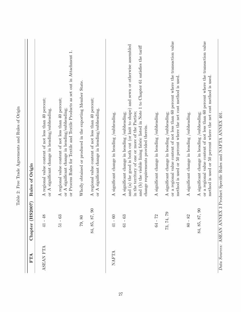
tariff rates. Rules of origin could be one of them. Rules of origin require that only the products

which are actually produced in the FTA region are qualified for preferential tariff rates. Each

free trade agreement assigns specific rules of origins for goods in each category. Table 2 lists the

product specific rules stated in ASEAN (Annex 3) and NAFTA (Annex 401). There are three main

methods of origin determination. The most strict one requires the products are wholly obtained or

produced in the exporting member state. The second sets a minimal percent of local value content

in the products. For instance, ASEAN FTA testifies the origin of a product if it contains 60 percent

or more regional value content, and NAFTA requires a regional value content of not less than 60

percent where the transaction value method is used or 50 percent where the net cost method is

used. The third method to confer origin is to show that the production taking place within the

region makes substantial transformation to the products so that its tariff heading or subheading is

changed. Considering the fact that most ASEAN countries undertake a great volume of production

along the global value chain, the rules of origin in ASEAN FTA is relatively strict.

All in all, rules of origin are an important part of an FTA and vary across products and across

FTAs. Strict rules of origin could be a reason for low FTA utilization rates, as it prevents goods

that contain high non-regional value content from being eligible for preferential tariffs, especially

in regions where countries have close vertical linkages in production with outside countries.

5

2.3 Administrative compliance and documentation costs offset tariff margin

attractiveness

In addition to the restrictiveness of ROOs, the costs of complying with the procedures of origin

certification are another reason for low FTA utilization rates. Rules of origin are often expensive

to document. Exporters must obtain a certificate from its national government and present it

to the customs authority of the importing government. Going through such an administrative

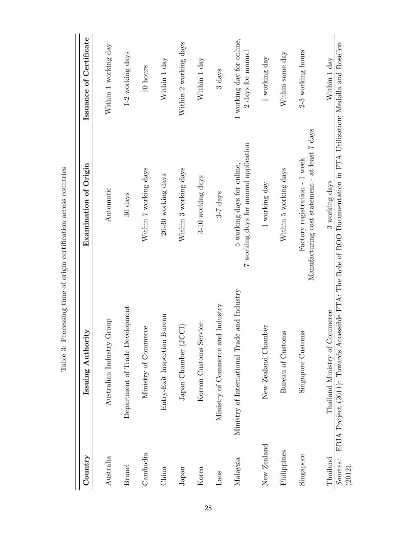
procedure makes the FTA preferences less attractive. Medalla and Rosellon (2012) conduct a

survey on the typical process for acquiring a certificate of origin. The pre-export verification requires

documentations like company registration, business license, organization code, etc. Processing time

from pre-export verification to issuance of certificate of origin ranges widely, from one working day

(as for Australia and New Zealand) to not more than 30 working days (as for China and Brunei).

Part of the survey results are reported in Table 3. It is the least costly to obtain a certificate

for exporters producing in Australia and New Zealand. The pre-export verification can be done

within one working day or automatically for electronic application. The entire processing time is

within a day. In the case of Korea and Japan, it takes about three working days to complete the

administrative procedure. For other countries, like Laos, China, and Malaysia, exporters have to

wait five to thirty working days to get a certificate.

Large fixed costs are another hurdle for FTA utilization, including learning about FTA pro-

visions and obtaining certificates of origin. Processing time for origin certification varies across

countries. Small and medium size exporters are less able to muster the requisite financial and

human resources than large firms, and therefore are less likely to utilize trade preferences. The

tariff margin attractiveness granted by an FTA is, at least partially, offset by documentation costs.

3 The Model

3.1 Set-up

Consider a free trade area consists of two countries: country A and country B. There are many

downstream firms producing final differentiated goods in both countries, and firm productivities

follow the same distribution. The only difference between the final good producers in the two coun-

tries lies in the sources of intermediate inputs. Country A is assumed not to produce intermediate

goods, and final good producers import intermediate goods from either country B or an outside

country, depending on import prices. In country B, there are upstream firms supplying intermediate

goods, and final good producers in that country choose to employ domestically produced inputs.

Differentiated final products can be sold to the other country at a zero tariff rate if the products

meet ROOs. As such, ROOs would affect the productions of exporters in country A only. Since this

paper focuses on the use of FTA, I assume away fixed costs of producing and exporting, meaning

that all firms are active exporters but export to the other country at different tariffs. Labor is

inelastically supplied and perfectly mobile between upstream and downstream firms. The model

6

builds on Melitz (2003), to which I add intermediate goods, tariff preferences and fixed costs of

using FTAs.

3.1.1 Preference

On the demand side, the preference of a representative consumer in country j (j = A, B) is given

by a nested Cobb-Douglas utility function:

Uj = Xαj H

1−αj (1)

where

Xj =

[∫Ωj

xij (ϕ)1−1/σ dϕ

]1/(1−1/σ)

.

Ω denotes the endogenous set of differentiated varieties sold in country j, xij (ϕ) is quantity

of variety ϕ produced in i and consumed in j, and the elasticity of substitution between any two

varieties within this industry is constant and equals σ > 1. Hj represents the consumption of

homogeneous goods in country j. Homogeneous goods can be traded freely across countries and

its price is normalized to be 1. α is the standard Cobb-Douglas parameter which stands for the

expenditure share on differentiated varieties. As in Dixit and Stiglitz (1977), the demand for variety

ϕ is given by

xij(ϕ) =αIj

P 1−σxj

pij (ϕ)−σ , (2)

where pij(ϕ) is the price of variety ϕ produced in i and sold in j, Ij is the representative con-

sumer’s income in country j, and Pxj is a price index of differentiated goods in j such that

Pxj = [∫ϕ∈Ωj

pij(ϕ)dϕ]1/(1−σ).

Under monopolistic competition, the optimal price for each variety is a constant mark-up over

unit cost. Hence, I have

pij (ϕ) =σ

σ − 1τijci (ϕ) , (3)

where ci (ϕ) denotes variety ϕ’s variable production costs in country i. τij > 1 is gross tariff rate

imposed by importing country j, and τii = 1.

3.1.2 Production in country A

Final goods X are produced using labor (La) and intermediate inputs. Since there are no upstream

firms in country A, final good producers import intermediate inputs from country B (Mb) and/or an

outside country C (Mc). The intermediate inputs originated from different countries are assumed to

be perfect substitutes, and how intensively the firm uses the imported inputs depends on the ROOs

and import prices. The production function takes a Cobb-Douglas form with constant returns to

scale:

7

xa (ϕ) = ϕ

(Mb +Mc

β

)β ( La1− β

)1−β,

where ϕ denotes a firm’s total factor productivity. Final good producers are heterogeneous in the

sense that they have different productivity draws from the Pareto distribution G(ϕ) = 1 − ϕ−ε,where ε measures the inverse of dispersion. A large value of ε implies that firms are less hetero-

geneous and the market structure is more competitive. Firms produce horizontally differentiated

final goods and each variety is indexed by ϕ ∈ [1, +∞]. To ensure there exists a closed solution,

I assume σ < ε + 1. β stands for the cost share of imported inputs in the production, which is

independent of wage rate and prices of intermediate inputs.

Firms take the prices of inputs as given. Without any additional restrictions, each firm chooses

labor and intermediate goods to minimize unit production costs:

minMb,Mc,La

pmbMb + pmcMc + waLa

s.t. xa (ϕ) > 1

Thus, the unconstrained unit production cost can be expressed as

ca (ϕ) =pβmcw

1−βa

ϕ. (4)

For simplicity, I assume the outside country C is more efficient than country B in producing

intermediate goods, so that pmb > pmc. The final good producers in country A initially choose

to import inputs from country C. The unconstrained unit cost is decreasing in productivity and

increasing in prices of inputs. Also, the cost share of foreign contents is β. Firms within one

industry differ in productivity and unit cost, but spend the same percentage of production costs

on intermediate inputs produced abroad.

Accordingly, the unconstrained unit demand for labor and the unconstrained unit demand for

intermediate goods are:

la =1− βϕ

(pmcwa

)β, (5)

Mc =β

ϕ

(wapmc

)1−β. (6)

3.1.3 Production in country B

In the intermediate good sector, labor is the only factor of production, and the products are sold in

a perfectly competitive market. Thus, I have the price of intermediate goods produced in country

B equals costs:

8

pmb =wbamb

, (7)

where wb is the wage rate in country B and amb is the labor efficiency in the production of inter-

mediate goods in country B.

Following the same production function as in country A, firms use labor and domestically

produced intermediate inputs to produce final products. The variable cost of producing 1 unit of

output is given by

cb (ϕ) =pβmbw

1−βb

ϕ. (8)

As shown in the cost equation, all inputs are sourced from domestic suppliers. Thus, the final

goods produced in country B automatically satisfy the rule of origin, no matter how strict it is. All

the exporters producing in country B would utilize the FTA preferences and export to country A

under zero tariff rates.

Moreover, country B also produces homogeneous goods, which are the numeraire goods in the

model. Producing 1 unit of homogeneous good requires1 unit of labor, and homogeneous goods

can be traded freely across countries. Hence, the wage rate in country B is normalized to be 1.

3.2 Utilizing FTAs

The preferences granted by the free trade agreement are conditional. To be qualified for zero tariffs,

final varieties must satisfy the ROO. Suppose the ROO requires the cost share of local contents

to be no less than γ and 0 < γ < 1. As such, the cost minimization problem for the firm with

productivity ϕ is subject to an additional constraint regarding the source of the inputs:

minMb,Mc,La

pmbMb + pmcMc + waLa

s.t. xa (ϕ) > 1

andpmcMc

pmbMb + pmcMc + waLa≤ 1− γ.

Then, the constrained unit production cost can be derived as

cac (ϕ) = λca (ϕ) (9)

where

λ =

1, if β 6 1− γ[

β(β+γ−1) pmc

pmb+1−γ

]β, if β > 1− γ.

(10)

9

λ measures the rise in unit production costs due to complying with ROO. If β 6 1 − γ, the

ROO is not binding. In this case, firms’ productions involves more domestic contents than the

requirement, therefore the second constraint of the optimization problem is automatically satisfied

and firms will stay with their optimal production plans. Comply with ROO does not generate

additional production costs, so λ = 1. If β > 1 − γ, the ROO is binding. That is, firms use more

foreign intermediate goods than the requirement. In this case, if firms intend to utilize the FTA

preferences, they need to deviates from their optimal production strategies by using more local

inputs to meet the ROO. Hence, λ > 1, and it increases with β and γ. The stricter the origin rule

is, the more the unit cost will increase by.

The corresponding constrained demands for labor and intermediate inputs are given by

lac (ϕ) = λla (ϕ) , (11)

and

Mcc = McC and Mb =β

ϕ

(wapmb

)1−βB, (12)

where C =(

1−γβ

)1−β[

1(β+γ−11−γ

)(pmcpmb

)+1

]β< 1 and B = β+γ−1

β

[β

β+γ−1+(1−γ)(pmbpmc

)]β

> 1.

Since the ROO requires more intensive use of locally produced inputs, the constrained demands

for labor and the intermediate goods from country B are greater than in the unconstrained case,

and they increase in the restrictiveness of ROO (γ). In contrast, the demand for the intermediate

goods originating from country C decreases as a binding ROO takes effect on firm production.

3.3 Partial equilibrium

Whether a firm chooses to utilize the preferential tariffs or not depends on the associated benefits

and costs. On the one hand, a firm would charge a lower price and make more sales in the foreign

market due to the tariff reductions. On the other hand, the distorted sourcing of inputs generates

extra production costs. Moreover, firms have to pay fixed documentation costs (fd) in order to

obtain a certificate of origin and claim the FTA preferences.

Assume there are no fixed costs of production and exporting. If the firm exports under the

MFN tariffs, it needs to pay a per unit tariff τij > 1 to access the foreign market. The profits are

revenues less costs in the domestic and the foreign markets. In particular, the profits of an FTA

non-user can be expressed as:

π1 = πad + πan =1

σpadxad +

1

στijpanxan, (13)

where πad, pad, and xad are firm’s profits, price, and quantity sold in the domestic market, and πan,

pan, and xan are firm’s profits, price, and quantity sold in the foreign market as an FTA non-user.

10

If a firm chooses to utilize the FTA preferences, it pays zero tariff, constrained unit costs, and

a positive fixed documentation cost. Hence, the corresponding profits of an FTA user is given by

π2 = πad + πaf =1

σpadqad +

1

σpafqaf − fdwa, (14)

where fixed documentation costs are paid in units of labor, and πaf , paf , and xaf are the firm’s

profits, price, and quantity sold in the foreign market as an FTA user. Comparing the profits of

FTA users and no-users, there is a tradeoff between optimizing the source of intermediate inputs

and having access to preferential tariffs, given that λ > 1 and τij > 1. Exporters would enjoy a

zero tariff at the expense of using more expensive inputs produced domestically. I assume λ < τ ,

the increase in unit cost due to ROO is smaller than the tariff margin. Otherwise, no one would

utilize the preferential tariffs offered by FTA.

From the individual firms’ perspective, it is the increased profits that motivate them to join the

FTA. Firms are willing to take advantage of zero tariffs if and only if π2 > π1. The productivity

threshold for utilizing FTA preferences should be the value which makes the firm indifferent between

being and not being an FTA user. That is, π1(ϕ∗) = π2(ϕ∗). Combining the conditions I have

derived above, the critical value is determined by

ϕ∗ =

[κf(wa)

σ−1fdλ1−σ − τ1−σ

] 1σ−1

(15)

where κ = σσ

(σ−1)σ−11

Pσ−1xb Ib

and f(wa) = pβmcw1−βa . κ represents the market demand condition in

the importing country, which is held constant in partial equilibrium analysis. A small value of

κ is associated with a large foreign market size (Ib) and a low price index (Pxb), both of which

indicate a strong market demand for variety ϕ. Similar to Melitz (2003), firms with different

productivities end up with different sales patterns. Only firms with productivities above the cutoff

ϕ∗ invoke the preferential tariffs while exporting. If λ1−σ − τ1−σ > κf(wa)σ−1fd, the FTA will

be fully utilized. All firms export under zero tariffs and make more revenues due to a lower trade

barrier: r2(ϕ) − r1(ϕ) > ( σσ−1)1−σ Ib

P 1−σxb

ca(ϕ)1−σκfd > 0, where r1(ϕ) and r2(ϕ) refer to export

revenues by not using and using FTA. If λ1−σ − τ1−σ < κfd , ϕ∗ > 1 follows. The FTA is

partially utilized. Firms with productivities smaller than the cutoff would export under the MFN

tariffs. The increase in exporting revenues induced by claiming the zero tariffs is still positive,

but it is much less than the revenue gains in the case with full utilization, since it can be shown:

0 < r2(ϕ) − r1(ϕ) < IbP 1−σxb

ca(ϕ)1−σκfd. Therefore, assuming full utilization of trade preferences

may overstate the role of FTAs in promoting bilateral trade.

The FTA utilization rate is the fraction of export value that takes advantage of the trade

agreement and pays lower tariffs. In this model, it is determined by the productivity threshold of

using FTA (ϕ∗):

11

u =

∫∞ϕ∗ r2(ϕ)dG(ϕ)∫ ϕ∗

1 r1(ϕ)dG(ϕ) +∫∞ϕ∗ r2(ϕ)dG(ϕ)

=1(

τλ

)1−σ [(ϕ∗)ε−σ+1 − 1

] (16)

As shown in (16), the larger the threshold is, the lower the utilization rate is. Thus, if an FTA

sets a large tariff margin, a loose ROO and simple administrative procedures, there will be a low

productivity threshold of utilizing FTA preferences and a high utilization rate. Also, the utilization

rate is relatively high in the industries where imported inputs account for a small cost share and it

is less costly to comply with ROOs.

4 General Equilibrium

Welfare analysis is approachable in a general equilibrium framework. In this section, I present a

general equilibrium model to investigate the welfare effects of ROOs and use GAMS to simulate the

results. Now consider a world comprised of three countries (A, B, and C). Two of them, country A

and country B, sign a free trade agreement in which countries permit zero import tariffs to exports

from the partner country if the products satisfy the ROO. Exporters producing in country A are

affected by ROOs. They have to reduce the use of inputs imported from country C in order to

be qualified for tariff benefits when the ROO is restrictive. Firms have different productivities

in producing differentiated final goods and they select themselves into profitable sales patterns.

Homogeneous goods are traded costlessly across countries in order to keep trade balanced. Since

the firm heterogeneity complicates the computation, I adopt the representation of the average firm

operating in each sale pattern, which is proposed by Balistreri and Rutherford (2011) and simplifies

the model effectively.

4.1 Country A

Country A is one of the participants of the free trade agreement. The labor endowment is denoted

as La. Workers in country A produce final differentiated goods. The documentation costs and the

firm entry costs are paid in units of labor. Workers are also consumers, and the utility function is

given by (1).

4.1.1 Production of final goods

As shown in the previous section, more productive firms choose to comply with the ROO and

export under zero tariffs. I assume the number of FTA non-users is n1 who stick with their original

production strategies and pay tariffs while exporting, and the rest n2 firms are FTA users. The

12

average productivity of FTA non-users is denoted by ϕ1 and the average productivity of FTA users

is ϕ2. Thus, the unit production costs for two types of firms are

c1(ϕ1) =pβmcw

1−βa

ϕ1(17)

and

c2(ϕ2) =λpβmcw

1−βa

ϕ2. (18)

Under monopolistic competition, heterogeneous firms set a constant markup over the unit costs

and the optimal prices for two groups of firms are given by

p1j =στijσ − 1

c1(ϕ1) (19)

and

p2j =σ

σ − 1c2(ϕ2). (20)

Accordingly, the demands for the average varieties in the two countries are

q1j =αIj p1j

−σ

P 1−σxj

, (21)

and

q2j =αIj p2j

−σ

P 1−σxj

, (22)

where Ij represents consumers’ total income in country j and Pxj stands for the price index of

differentiated goods in country j. The corresponding profits earned by firms can be expressed by

π1j =1

σp1j q1j (23)

and

π2j =1

σp2j q2j − fdwa. (24)

The indifference condition for the marginal firm can be derived in terms of the average FTA

user’s revenues and the parameters by linking the average FTA user’s and nonuser’s productivities

and revenues to the marginal firm through the Pareto distribution. The equivalent condition to

the cutoff condition (15) is given by the equation below:

1

σ

ε+ 1− σε

[1−

(τλ

)1−σ]p2q2 = fdwa. (25)

Moreover, the free entry condition drives firms’ profits down to zero:

∑j=A,B

π1j =∑j=A,B

π2j = wafe (26)

13

The productivity of the marginal exporter and the fraction of FTA users can be linked by

n2 = 1 − G (ϕ∗). With this relationship, I can express the average productivities of nonusers and

users in terms of the number of exporters using FTA as

ϕ1 =

ε

ε+ 1− σ1− n

ε+1−σε

2

1− n2

1σ−1

(27)

and

ϕ2 =

(ε

ε+ 1− σ

) 1σ−1

n− 1ε

2 . (28)

4.1.2 Labor market and income balance

The labor market clearing condition is

La = n1la∑j=A,B

q1j + n2 ( ˜q2ala + q2blac) + nafe + n2fd (29)

where na = n1 + n2 is the total number of firms producing in country A, and n1 and n2 are the

number of FTA non-users and users respectively. fe is the units of labor required to hire to enter

the market. Labor demand consists of four parts: the demand by FTA non-users and users to

produce outputs, the demand by all active firms to pay entry costs, and the demand by FTA users

to pay documentation costs.

Following the free entry condition, consumer’s total income is wage payment. Therefore, the

income balance condition is

Ia = waLa. (30)

4.2 Country B

Country B, the second participant in the FTA, produces and exports to country A differentiated

goods and homogeneous goods H (pH = 1). The labor endowment is Lb. Consumers’ utility is

derived over a continuum of differentiated varieties and homogeneous goods.

All exports originating from country B satisfy the ROO and claim preferential tariffs. The free

entry condition for firms producing in country B implies that

πb =1

σpb∑j=A,B

qbj = fbwb, (31)

where πb, pb, and qbj are the profits, price, and quantity of the average exporter in country B. fb

is the entry costs in country B and is paid by labor. Since all exports from country B are qualified

for zero tariffs, firms charge the same price in the domestic and the foreign markets.

The labor market clearing condition equates labor supply and demand:

14

Lb = nblb∑j=A,B

qbj + nbfb +n2qafMb

amb+ hbp, (32)

where nb is total number of exporters from country B, lb is the labor demand by producing 1 unit of

differentiated good, and hbp is the quantity of homogeneous goods produced in country B. Country

B conducts three production activities. The first two terms on the right hand side of (32) indicate

the labor demand by firms producing final goods. The third term is the labor working in the

intermediate good sector, and the last term is the labor demand in the production of homogeneous

goods.

Country B’s total income comes from two sources. One is labor income by producing differenti-

ated and homogeneous goods, and the other is import tariff revenues imposed on country A’s FTA

non-users. The income balance condition is

Ib = wbLb +τ − 1

τn1p1bq1b. (33)

4.3 Country C

Country C is the outside country. The labor endowment is Lc. People living country C produce

intermediate inputs (Mc) and export them to country A. The intermediate inputs are produced

using labor only and sold in a perfectly competitive market at the price of pmc = wcamc

. Country C

also produces homogeneous goods, and therefore the wage rate is normalized to be one. There are

no consumption and production of differentiated goods in country C. Homogeneous goods are the

only consumption goods.

The labor supply-equal-demand condition yields

Lc = n1Mc

∑j=A,B

q1j + n2Mc ˜q2a + n2Mccq2b + hcp, (34)

where ˜q2a and q2b are the quantities of outputs sold by the average FTA user in country A and

country B, and hcp is the amount of homogeneous goods produced in country C. A binding ROO

forces FTA users to switch from foreign to local intermediate inputs so that the unit demand for

intermediate goods originating from country C by FTA users is smaller than by non-usersMcc < Mc.

The total income can be expressed as

Ic = Lcwc. (35)

4.4 Closing the model

The trade and payment systems are closed by trade balance conditions. Country A produces and

exports differentiated goods to country B under either zero or the MFN tariff rates. It imports

intermediate inputs from country B and country C. Country A’s imports of final products from

15

country B are under zero tariffs. To keep trade balanced, country A also imports homogeneous

goods. The trade balance condition equates value of exports with value of imports:

n1p1bq1b

τ+ n2p2bq2b = nbpbqba + IMmc + IMmb + pHhaim (36)

where

IMmc = pmc

n1Mc

∑j=A,B

q1j + n2Mc ˜q2a + n2Mccq2b

IMmb = pmbn2q2bMb.

IMmc and IMmb represent the value of imported intermediate inputs from country C and country

B respectively. ha is the consumption of homogeneous goods in country A. The left hand side of

(36) is the exporting revenues earned by FTA non-users and users, and the right hand side is the

sum of import values.

Country B makes export revenues by selling differentiated goods and intermediate inputs to

country A under zero tariffs as well as homogeneous goods. The tariff payments from country A’s

FTA non-users are redistributed to country B’s consumers. The trade balance condition for country

B is

nbpbqba +τ − 1

τn1p1bq1b + EXmb + pHhbex = n1p1bq1b + n2p2bq2b, (37)

where EXmb = IMmb is the export value of intermediate inputs from country B to country A. hbex

is quantity of homogeneous goods exported from country B, which could be negative if country B

imports homogeneous goods.

Country C consumes homogeneous goods only and conduct productions of intermediate inputs

and homogeneous goods. The trade balance conditions comes as

EXmc = pHhcim, (38)

where EXmc = IMmc stands for the value of intermediate goods exported from country C to

country A. hcim is the amount of homogeneous goods imported by country C to keep trade balanced.

Also, hcim should be equal to the difference between country C’s consumption and production of

homogeneous goods.

Lastly, the world demand and supply of homogeneous goods are equalized. The market clearing

condition for the homogeneous goods is

hcim + haim = hbex. (39)

16

4.5 Equilibrium

So far, every dollar paid is a dollar of revenue earned. Given σ, α, β, τ , amc, amb and productivity

distribution G (ϕ), an equilibrium is a set of numbers of firms (n1, n2, nb), aggregate price statistics

(Pxa, Pxb), wage rate wa, consumer allocations qij (i = 1, 2, b and j = a, b), firm pricing rules pb

and pib(i = 1, 2), firm profits πij (i = 1, 2, b and j = a, b), and homogeneous good trade value

(haim, hbex, hcim), such that: (i) qij is given by (21) (22) and solves the representative consumer’s

problem; (ii) pb and pib are given by (19) (20) and solves the firm’s problem; (iii) πij is given by

(23)(24); (iv) n1, n2, nb, Pxa, Pxb, wa, qij , haim, hbex, hcim jointly satisfy (25)-(39).

There are no analytical solutions to this complicated system of equations. I adopt two ap-

proaches to make a progress. First, I conduct comparative static exercise in the neighborhood of

full utilization and show the local analytical results. Second, I take advantage of GAMS program

to provide global numerical solutions.

5 Local Analytical Solutions and Welfare Analysis

In this section, I conduct comparative static exercise in the neighborhood of full utilization. The

results show the local effects of a slightly binding rule of origin on market outcomes and welfare.

Consider the equilibrium in which the ROO is exactly satisfied by the Cobb-Douglas cost share

of imported inputs, that is β = 1 − γ. Now if there is a slight increase in the local content

requirement (ROO), the ROO starts being binding. The producers in country A are faced with

choices of whether to utilize the trade preferences. The endogenous variables of the model would

change accordingly.

5.1 Number of producers

The percentage change of number of FTA users in country A can be expressed as

n2 = −σ − 1

x

[1

(β + σ (1− β)) (1 + y/τσ) sf+τσ (1 + 1/y)

τσ − 1

1

sf− 1

]︸ ︷︷ ︸

(+)

λ, (40)

where x =(fdfe

+ 1) [ατ−σ (τ − 1)− τ1−σ + 1

]> 0 and y = fe

fd(τσ − 1)− 1 > 0. sf =

n2p1−σ2b

P 1−σxb

is the

market share of exports by FTA users in country B. n2 = dn2n2

and λ = dλλ represent the percentage

changes of number of FTA users and ROO. The effect of a slightly binding ROO on firm production

is fully reflected in the change of variable costs λ. Thus, (40) states a negative relationship between

number of FTA users and the restrictiveness of ROO. As λ increases, n2 decreases. The total

number of exporters originating from country A is negatively correlated with the number of FTA

users, since I have

na = −fdfen2. (41)

17

Considering that the number of FTA non-users is equal to the total number less the number of

users (n1 = na−n2), a stricter ROO leads to an increase in total number of exporters producing in

country A, an increase in number of FTA non-users, and a decrease in number of FTA users. This

is consistent with the intuition. When the ROO requires more local inputs, exporters in country

A have to alter their productions and produce at a higher cost. The trade preferences are costly

to utilize, which results in an exit from being FTA users.

par As for the change in number of exporters producing in country B, it can be seen from

nb =σ − 1

1− sf

[σ + (1− σ)sf

(1 + y/τσ) (σ + β/(1− β))+ 1− τσ

τσ − 1

]λ. (42)

Given that σ > 1, sf < 1, and the sign of the bracket is positive, nb and λ are positively

correlated. As the ROO becomes tighter, more producers in country B start exporting to country

A. This is due to the fact that a higher requirement of local content disadvantages producers in

country A. More exporters from country B benefit from the preferential tariffs and make sales in

the foreign market.

5.2 Wage rate

In such a framework, country A can be thought of Mexico in NAFTA. An interesting and important

question is how the implementation of NAFTA and ROOs affects the wage rate in Mexico. The

local comparative static analysis shows that

wa = − σ − 1

(1 + y/τσ) (β + σ (1− β))λ. (43)

When the ROO increases, there are two opposing factors that influences labor demand. On

the intensive margin, FTA users demand more labor and local inputs to meet the ROO. On the

extensive margin, the trade preferences will be utilized by fewer exporters. For those who exported

under preferential tariffs before, an exit from the FTA framework leads to a reduction in the demand

for local inputs, since they no longer need to comply with the rule. (43) shows that the overall

effect is negative. An increase in ROO (λ) leads to a decrease in the wage rate of the downstream

country (wa).

5.3 Price index

The change in ROO reallocates sales of heterogeneous firms. As a result, the price indexes in the

FTA participating countries change. Both domestic firms and exporters from country B sell in

country A. The price index in country A is given by

P 1−σxa = nap

1−σa + nbp

1−σb .

Accordingly, the percentage change in price index caused by the change in ROO is

18

Pxa = −1− sbσ − 1

na −sb

σ − 1nb︸ ︷︷ ︸

variaty effect(−)

+ (1− sb) ˆpa︸ ︷︷ ︸price effect(−)

, (44)

where sb =nbp

1−σb

P 1−σxa

denotes the market share of exports from country B in country A. The effect

of ROO on price index can be decomposed into two parts. One is variety effect in that a stricter

ROO leads more firms to start producing in and exporting to both countries, which drives down

the price index and intensifies market competition. The other effect is price index. The domestic

producers in country A would charge lower prices following a binding ROO, because the wage rate

goes down, as discussed in the previous section. Hence, both variety effect and price effect are

negative. An increase in local content requirement reduces the price index in country A.

Similarly, in country B, there are three types of producers supplying differentiated goods. The

associated price index is

P 1−σxb = n1p

1−σ1b + n2p

1−σ2b + nbp

1−σb .

Total differentiating with respect to rules of origin yields

Pxb = −1− (1 + fd/fe) τ1−σ

σ − 1sf n2︸ ︷︷ ︸

(+)

+ (1− sf )nb

1− σ︸ ︷︷ ︸(−)

+ sf ˆp2b︸ ︷︷ ︸(+)

. (45)

The sign of the percentage change in price index in country B is ambiguous, depending on the

market share of country A’s exporters in country B. If the export sales of FTA users account for

a large market share in country B, the positive variety effect driven by fewer FTA users and the

positive price effect dominate. Thus, country B’s price index Pxb increases in ROO. If the export

sales of FTA users account for a small market share in country B, the negative variety effect due

to the firm entry in country B outweighs the other two effects, which decreases the price index Pxb

as the ROO rises.

5.4 Welfare

Country welfare is jointly determined by income and price index. A country with more income and

a lower price index has a higher welfare level. Specifically, country A’s welfare change due to a

binding ROO is

ˆWelfarea =

(1

1− β− (1− sb)

)ˆpa︸ ︷︷ ︸

TOT (−)

+1− sbσ − 1

(nb + na)︸ ︷︷ ︸variety effect(+)

. (46)

As shown in (46), the terms of trade effect and the variety effect run in the opposite directions.

On the one hand, country A’s exports become cheaper relative to its imports from country B,

because a binding ROO generates distortions in the labor market, which reduces the wage rate. On

19

the other hand, there are more varieties sold in country A, since an increase in ROO encourages

firm entry. It can be shown that if τσ

λσ−1 > 1 + fdfe

is satisfied and the elasticity of substitution

between varieties is small, the variety effect dominates. In other words, if the FTA is under-utilized

and varieties are less substitutable, country A’s welfare rises with the restrictiveness of ROO, as a

wider range of varieties are sold in the market. If the elasticity of substitution between varieties is

large, the magnitude of variety effect is small. In such a case, the overall effect of ROO on country

A’s welfare is negative, with the terms of trade effect more than offsetting the variety effect.

The percentage change in country B’s welfare due to a tighter ROO can be expressed as

ˆWelfareb =(τ − 1) y

τσsfn1 + (1− sf )

nbσ − 1

− sf ˆp2b +1− (1 + fd/fe) τ

1−σ

σ − 1sf n2. (47)

The analysis of country B’s welfare involves three channels. In terms of income, as the ROO

become tighter, country B’s tariff revenues increase, since more of exporters from country A choose

to be FTA non-users and pay import tariffs. In the meantime, country’s B wage rate is normalized

to be 1. Hence, the income effect is positive. The second channel is through the terms of trade

effect. Firms producing in country B are not affected by ROO and the wage rate is fixed, therefore,

the prices of exports remain the same. But country A’s production costs drop, which results in a

decrease in the average price of its exports. Facing a higher relative price of exports to imports,

country B’s welfare rises. Lastly, the sign and the magnitude of variety effect vary with the elasticity

of substitution between varieties as well as the market share of country A’s exports in country B.

Thus, the overall effect of ROO on country B’s welfare is ambiguous.

As we can see in (47), total differentiation yields a complicated expression for the percentage

change in welfare. There are three types of firms supplying differentiated goods in country B, and

the prices and the numbers of these firms change with ROO. Based on the analytical solution, I

can hardly conclude the direction towards which welfare moves following a stricter ROO. I resort

to numerical approach to pin down the relationship between country welfare and ROO.

6 Simulation results

In this section, I take advantage of GAMS program to show global numerical solutions to the

model. The results present the effects on key endogenous variables over a full range of ROOs.

In the benchmark, I assume the parameters take on the following values: the shape parameter of

Pareto distribution ε = 5, the elasticity of substitution between varieties σ = 4, the expenditure

share on differentiated varieties α = 0.8, the cost share parameters of Cobb-Douglas production

function β = 0.8, the local content requirement (ROO) γ = 0.2, the gross import tariffs τ = 1.3,

the benchmark wage rates in three countries are equal wA = wB = wc = 1, and the efficiency

parameters of producing intermediate inputs in countries B and C amb = 0.9 and amc = 1. The

fixed documentation costs, fixed entry costs in countries A and B, and the labor endowments in

three countries can be calibrated from the model.

Table 4 reports the results for the benchmark. The free trade agreement offers a 30% tariff

20

reduction to final varieties whose cost shares of domestically produced inputs are no less than 80%.

In the benchmark, since β = 1− γ, the rule of origin is not binding. There are 20 firms exporting

from A to B, and all of them utilize the preferential tariffs. The FTA utilization rate is 100 percent.

The number of exporters originating from country B is 20. The outside country C is more efficient

in producing intermediate inputs. When the ROO is loose, firms in country A source inputs from

country C only. The import value of intermediate inputs from C to A is 11.62, and the import

value of intermediate inputs from B to A is 0. The benchmark welfares in countries A and B are

10.35 and 26.72 respectively.

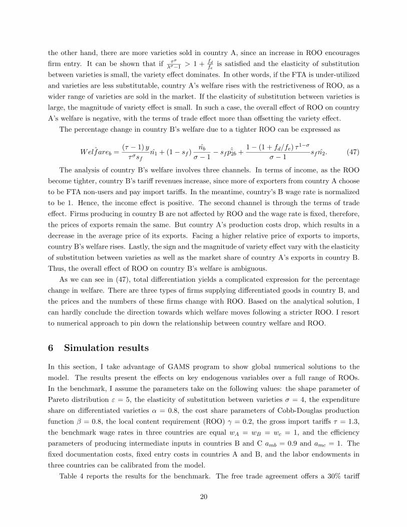
Next, I conduct counterfactual exercises to investigate the impacts of ROOs on country’s welfare

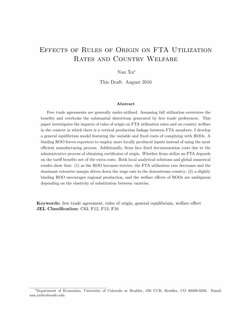
over the range from 1% to 95%. Figure 1 shows the simulation results on the use of FTA by country

A exporters. In panel (a), the number of FTA non-users is 0 when the ROO is 20% or below. It

rises from 0 to 37.63 gradually when the ROO increases from 20% to 59%. Since all firms choose

to be non-users if the local content requirement is 59% or even higher, the number of FTA non-

users remain the constant when the ROO is greater than 59%. In contrast, the number of FTA

users moves in the opposite direction. There is a monotonic decreasing trend over the range of

ROO from 20% to 59%, as shown in panel (b). As it is more and more costly for firms to comply

with the ROO, fewer exporters find profitable to utilize the trade preferences. Panel (c) displays

the relationship between FTA utilization rate and ROO. When the ROO is loose, the utilization

rate is 100 percent. As the ROO increases, the utilization rate decreases monotonically. Once the

local content requirement is too restrict (beyond 59%), none of the exporters take advantage of the

preferential tariffs and the utilization rate is zero.

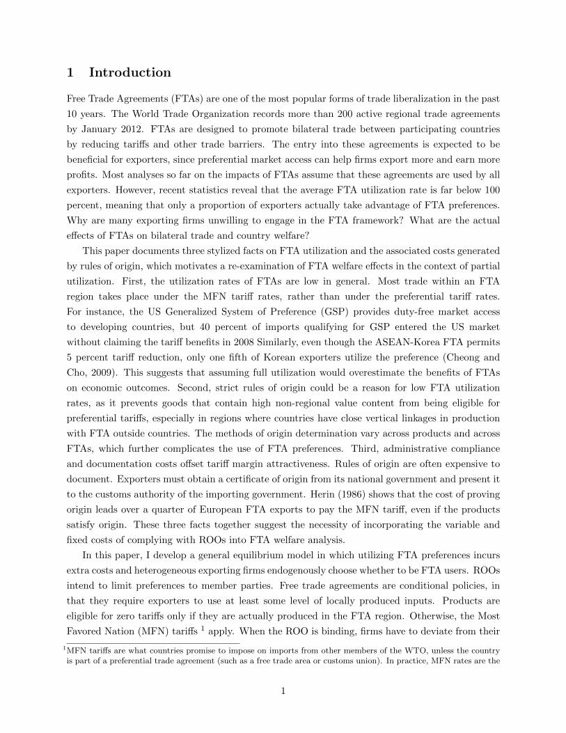
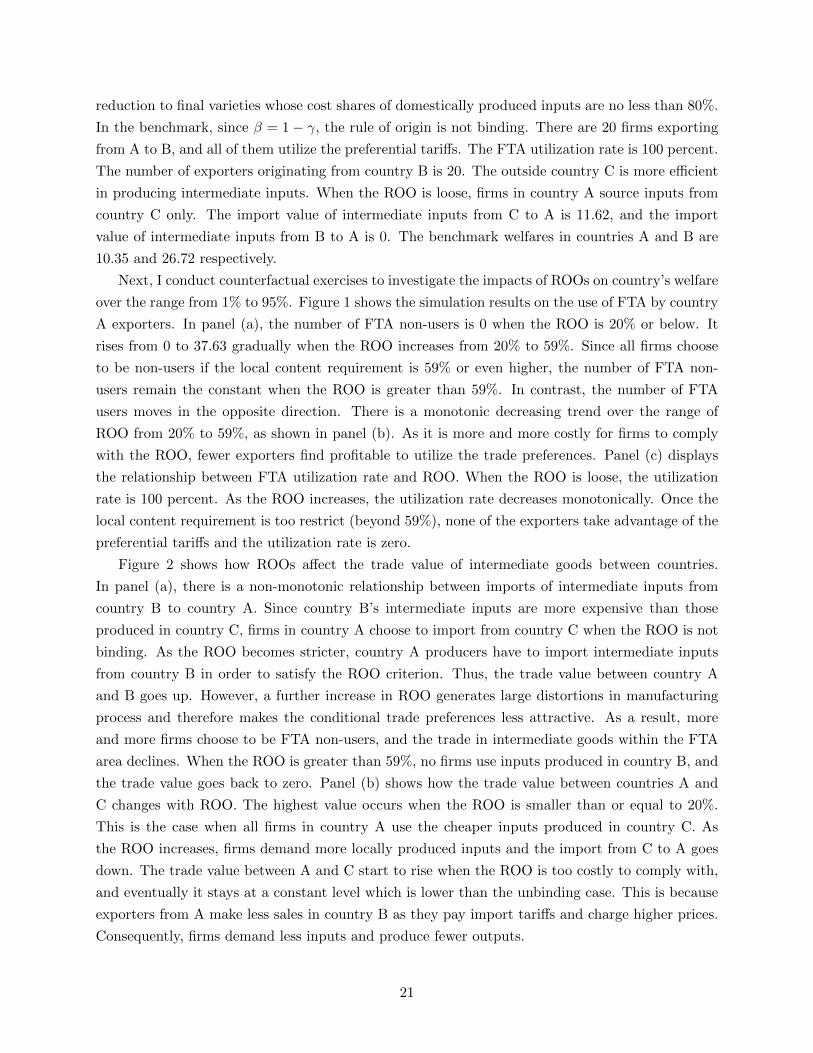
Figure 2 shows how ROOs affect the trade value of intermediate goods between countries.

In panel (a), there is a non-monotonic relationship between imports of intermediate inputs from

country B to country A. Since country B’s intermediate inputs are more expensive than those

produced in country C, firms in country A choose to import from country C when the ROO is not

binding. As the ROO becomes stricter, country A producers have to import intermediate inputs

from country B in order to satisfy the ROO criterion. Thus, the trade value between country A

and B goes up. However, a further increase in ROO generates large distortions in manufacturing

process and therefore makes the conditional trade preferences less attractive. As a result, more

and more firms choose to be FTA non-users, and the trade in intermediate goods within the FTA

area declines. When the ROO is greater than 59%, no firms use inputs produced in country B, and

the trade value goes back to zero. Panel (b) shows how the trade value between countries A and

C changes with ROO. The highest value occurs when the ROO is smaller than or equal to 20%.

This is the case when all firms in country A use the cheaper inputs produced in country C. As

the ROO increases, firms demand more locally produced inputs and the import from C to A goes

down. The trade value between A and C start to rise when the ROO is too costly to comply with,

and eventually it stays at a constant level which is lower than the unbinding case. This is because

exporters from A make less sales in country B as they pay import tariffs and charge higher prices.

Consequently, firms demand less inputs and produce fewer outputs.

21

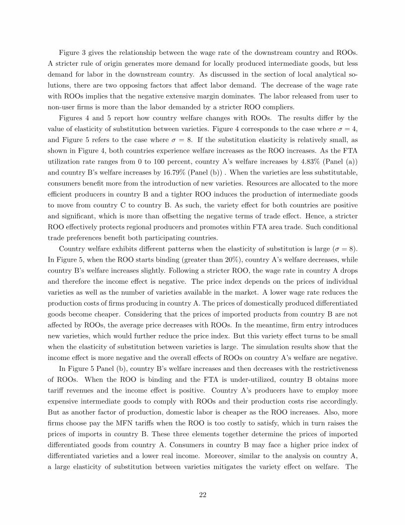
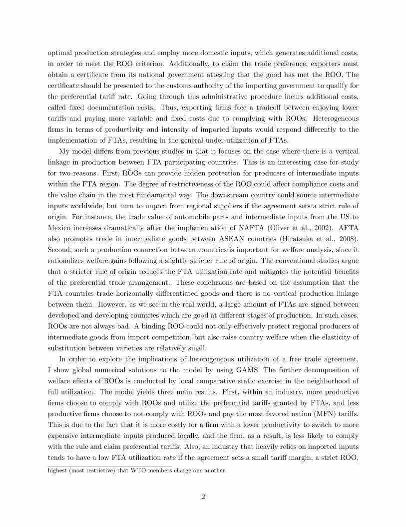
Figure 3 gives the relationship between the wage rate of the downstream country and ROOs.

A stricter rule of origin generates more demand for locally produced intermediate goods, but less

demand for labor in the downstream country. As discussed in the section of local analytical so-

lutions, there are two opposing factors that affect labor demand. The decrease of the wage rate

with ROOs implies that the negative extensive margin dominates. The labor released from user to

non-user firms is more than the labor demanded by a stricter ROO compliers.

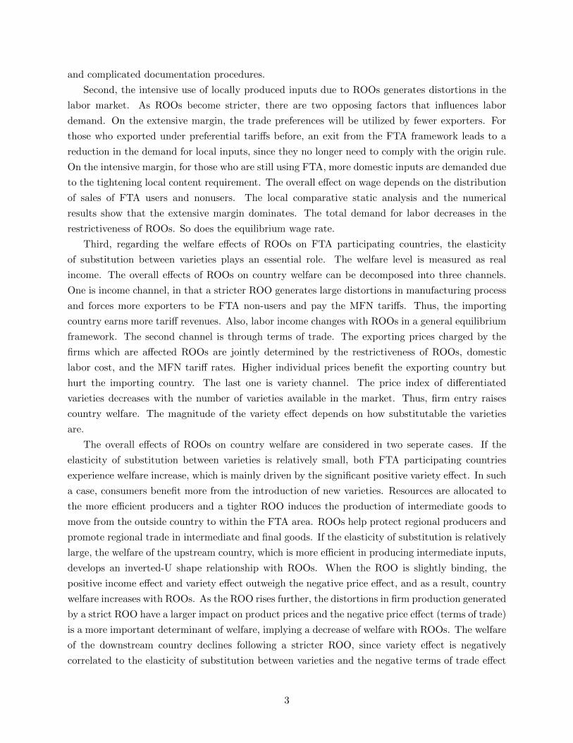
Figures 4 and 5 report how country welfare changes with ROOs. The results differ by the

value of elasticity of substitution between varieties. Figure 4 corresponds to the case where σ = 4,

and Figure 5 refers to the case where σ = 8. If the substitution elasticity is relatively small, as

shown in Figure 4, both countries experience welfare increases as the ROO increases. As the FTA

utilization rate ranges from 0 to 100 percent, country A’s welfare increases by 4.83% (Panel (a))

and country B’s welfare increases by 16.79% (Panel (b)) . When the varieties are less substitutable,

consumers benefit more from the introduction of new varieties. Resources are allocated to the more

efficient producers in country B and a tighter ROO induces the production of intermediate goods

to move from country C to country B. As such, the variety effect for both countries are positive

and significant, which is more than offsetting the negative terms of trade effect. Hence, a stricter

ROO effectively protects regional producers and promotes within FTA area trade. Such conditional

trade preferences benefit both participating countries.

Country welfare exhibits different patterns when the elasticity of substitution is large (σ = 8).

In Figure 5, when the ROO starts binding (greater than 20%), country A’s welfare decreases, while

country B’s welfare increases slightly. Following a stricter ROO, the wage rate in country A drops

and therefore the income effect is negative. The price index depends on the prices of individual

varieties as well as the number of varieties available in the market. A lower wage rate reduces the

production costs of firms producing in country A. The prices of domestically produced differentiated

goods become cheaper. Considering that the prices of imported products from country B are not

affected by ROOs, the average price decreases with ROOs. In the meantime, firm entry introduces

new varieties, which would further reduce the price index. But this variety effect turns to be small

when the elasticity of substitution between varieties is large. The simulation results show that the

income effect is more negative and the overall effects of ROOs on country A’s welfare are negative.

In Figure 5 Panel (b), country B’s welfare increases and then decreases with the restrictiveness

of ROOs. When the ROO is binding and the FTA is under-utilized, country B obtains more

tariff revenues and the income effect is positive. Country A’s producers have to employ more

expensive intermediate goods to comply with ROOs and their production costs rise accordingly.

But as another factor of production, domestic labor is cheaper as the ROO increases. Also, more

firms choose pay the MFN tariffs when the ROO is too costly to satisfy, which in turn raises the

prices of imports in country B. These three elements together determine the prices of imported

differentiated goods from country A. Consumers in country B may face a higher price index of

differentiated varieties and a lower real income. Moreover, similar to the analysis on country A,

a large elasticity of substitution between varieties mitigates the variety effect on welfare. The

22

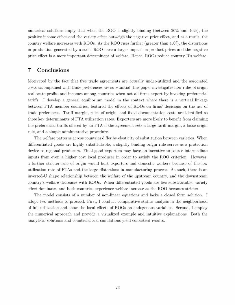
numerical solutions imply that when the ROO is slightly binding (between 20% and 40%), the

positive income effect and the variety effect outweigh the negative price effect, and as a result, the

country welfare increases with ROOs. As the ROO rises further (greater than 40%), the distortions

in production generated by a strict ROO have a larger impact on product prices and the negative

price effect is a more important determinant of welfare. Hence, ROOs reduce country B’s welfare.

7 Conclusions

Motivated by the fact that free trade agreements are actually under-utilized and the associated

costs accompanied with trade preferences are substantial, this paper investigates how rules of origin

reallocate profits and incomes among countries when not all firms export by invoking preferential

tariffs. I develop a general equilibrium model in the context where there is a vertical linkage

between FTA member countries, featured the effects of ROOs on firms’ decisions on the use of

trade preferences. Tariff margin, rules of origin, and fixed documentation costs are identified as

three key determinants of FTA utilization rates. Exporters are more likely to benefit from claiming

the preferential tariffs offered by an FTA if the agreement sets a large tariff margin, a loose origin

rule, and a simple administrative procedure.

The welfare patterns across countries differ by elasticity of substitution between varieties. When

differentiated goods are highly substitutable, a slightly binding origin rule serves as a protection

device to regional producers. Final good exporters may have an incentive to source intermediate

inputs from even a higher cost local producer in order to satisfy the ROO criterion. However,

a further stricter rule of origin would hurt exporters and domestic workers because of the low

utilization rate of FTAs and the large distortions in manufacturing process. As such, there is an

inverted-U shape relationship between the welfare of the upstream country, and the downstream

country’s welfare decreases with ROOs. When differentiated goods are less substitutable, variety

effect dominates and both countries experience welfare increase as the ROO becomes stricter.

The model consists of a number of non-linear equations and lacks a closed form solution. I

adopt two methods to proceed. First, I conduct comparative statics analysis in the neighborhood

of full utilization and show the local effects of ROOs on endogenous variables. Second, I employ

the numerical approach and provide a visualized example and intuitive explanations. Both the

analytical solutions and counterfactual simulations yield consistent results.

23

References

[1] Balistreri, Edward, Russell H. Hillberry, and Thomas F. Rutherford. “Structural

estimation and solution of international trade models with heterogeneous firms.” Journal of

International Economics, 2011, 83(2), pp. 95-108

[2] Brenton, Paul and Miriam Manchin. “Making EU Trade Agreements Work: The Role of

Rules of Origin.” The World Economy, 2003, 26(5), pp. 755-769

[3] Cadot, Oliver, Jamie de Melo, Akiki Suwa Eisenmann and Bolormaa Tu-

murchudur. “Assessing the Effect of NAFTAs Rules of Origin. ” Mimeo, 2002

[4] Cadot, Oliver, Jaime De Melo, and Alberto Portugal-Perez. “Rules of origin for

preferential trading arrangements : implications for the ASEAN Free Trade Area of EU and

U.S. experience.” Journal of Economic Integration, 2008, 22, pp. 256-287

[5] Cheong, Inkyo and Jungran Cho. “An Empirical Study on the Utilization Ratio of FTAs

by Korean Firms.” Journal of Korea Trade, 2009, 13(2), pp. 109-126

[6] Cherkashin, Ivan, Svetlana Demidova, Hiau Looi Kee, and Kala Krishna. “Firm

Heterogeneity and Costly Trade: A New Estimation Strategy and Policy Experiments.” NBER

Working Papers 16557, 2009

[7] Demidova, Svetlana, Hiau Looi Kee, and Kala Krishna. “Do Trade Policy Differences

Induce Sorting? Theory and Evidence from Bangladeshi Apparel Exporters.” Journal of Inter-

national Economics, 2012, 87(2), pp. 247-261.

[8] Eaton, Jonathan, Samuel Kortum, and Francis Kramarz. “Dissecting Trade: Firms,

Industries, and Export Destinations.” American Economic Review, 2004, 94(2), pp. 150-154

[9] Foster, Lucia, John Haltiwanger, and Chad Syverson. “Reallocation, Firm Turnover,

and Efficiency: Selection on Productivity or Profitability?” American Economic Review, 2008,

98(1), pp. 394-425.

[10] Hayakawa, Kazunobu. “Impacts of FTA Utilization on Firm Performance.” IDE Discussion

Paper No. 366, 2012

[11] Hayakawa, Kazunobu, Hansung Kim, and Hyun-Hoon Lee. “Determinants on Utiliza-

tion of Korea-ASEAN Free Trade Agreement: Margin Effect, Scale Effect, and ROO Effect.”

BRC Research Report No.9, 2010

[12] Hayakawa, Kazunobu, Daisuke Hiratsuka, Kohei Shiino, and Seiya Sukegawa.

“Who Uses Free Trade Agreements?” Asian Economic Journal, 2013, 27(3), pp. 245-264

[13] Herin, Jan. “” Rules of Origin and Differences between Tariff Levels in EFTA and in the

EC., 1986, EFTA Occasional Paper No. 13

[14] Hiratsuka, Daisue, Kazunobu Hayakawa, Kohei Shino, and Seiya Sukegawa. “Max-

imizing Benefits from FTAs in ASEAN.” ERIA Research Project Report, 2008(1), pp. 407-545

[15] Ju, Jiandong and Kala Krishna. “Firm Behavior and Market Access in a Free Trade Area

with Rules of Origin.” Canadian Journal of Economics, 2005, 38(1), pp. 290-308

[16] Keck, Alexander and Andreas Lendle. “New Evidence on Preference Utilization.” The

WTO Working Paper, No.ERSD-2012-12, 2012

24

[17] Lopez-Silanes, Florencio, James R. Markusen, and Thomas F. Rutherford. “Trade

policy subtleties with multinational firms.” European Economic Review, 1996, 40, pp.1605-1627

[18] Medalla, Erlinda and Maureen Rosellon. “Rules of Origin in ASEAN+1 FTAs and

the Value Chain in East Asia.” Discussion paper series No. 2012-37, Philippine Institute for

Development Studies, 2012

[19] Melitz, Marc J. “The Impact of Trade on Intra-Industry Reallocations and Aggregate

Industry Productivity.” Econometrica, 2003, 71(6), pp. 1695-1725.

[20] Melitz, Marc J., and Gianmarco Ottaviano. “Market Size, Trade, and Productivity.”

Review of Economic Studies, 2008, 75(1), pp. 295-316.

[21] Menon, Jayant. “Preferential and Non-Preferential Approaches to Trade Liberalization in

East Asia: What Differences Do Utilization Rates and Reciprocity Make?” ADB Working Paper

Series on Regional Economic Integration, No. 109, 2013

[22] Oyamada, Kazuhiko. “Parameterization of Applied General Equilibrium Models with Flex-

ible Trade Specifications Based on the Armington, Krugman, and Melitz Models.” IDE Dis-

cussion Papers 380, 2013, Institute of Developing Economies, Japan External Trade Organiza-

tion(JETRO)

[23] Roberts, Mark, and James Tybout. “Sunk Costs and the Decision to Export in Colom-

bia.” American Economic Review, 1997, 87(4), pp. 545-564.

[24] Tybout, James. “Plant and Firm Level Evidence on ”New” Trade Theories.” In J.Harrigan

Ed. Handbook of International Economics, Basil Blackwell., 2002.

25

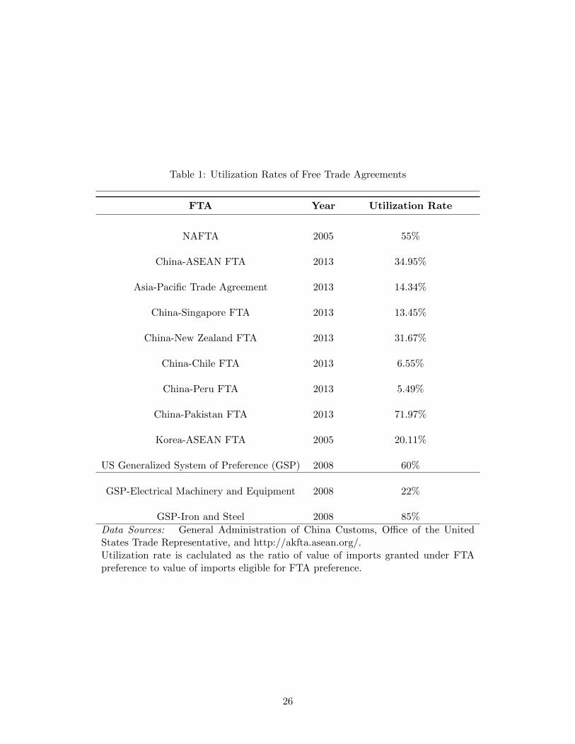
Table 1: Utilization Rates of Free Trade Agreements

FTA Year Utilization Rate

NAFTA 2005 55%

China-ASEAN FTA 2013 34.95%

Asia-Pacific Trade Agreement 2013 14.34%

China-Singapore FTA 2013 13.45%

China-New Zealand FTA 2013 31.67%

China-Chile FTA 2013 6.55%

China-Peru FTA 2013 5.49%

China-Pakistan FTA 2013 71.97%

Korea-ASEAN FTA 2005 20.11%

US Generalized System of Preference (GSP) 2008 60%

GSP-Electrical Machinery and Equipment 2008 22%

GSP-Iron and Steel 2008 85%

Data Sources: General Administration of China Customs, Office of the UnitedStates Trade Representative, and http://akfta.asean.org/.Utilization rate is caclulated as the ratio of value of imports granted under FTApreference to value of imports eligible for FTA preference.

26

Tab

le2:

Fre

eT

rad

eA

gree

men

tsan

dR

ule

sof

Ori

gin

FT

AC

hap

ter

(HS

2007)

Ru

les

of

Ori

gin

AS

EA

NF

TA

41

-48

Are

gion

alva

lue

conte

nt

ofn

otle

ssth

an40

per

cent;

orA

sign

ifica

nt

chan

gein

hea

din

g/su

bh

ead

ing.

51-

63

Are

gion

alva

lue

conte

nt

ofn

otle

ssth

an40

per

cent;

orA

sign

ifica

nt

chan

gein

hea

din

g/su

bh

ead

ing;

orP

roce

ssR

ule

sfo

rT

exti

lean

dT

exti

leP

rod

uct

sas

set

out

inA

ttac

hm

ent

1.

79,

80W

hol

lyob

tain

edor

pro

du

ced

inth

eex

por

tin

gM

emb

erS

tate

.

84,

85,

87,

90A

regi

onal

valu

eco

nte

nt

ofnot

less

than

40p

erce

nt;

orA

sign

ifica

nt

chan

gein

hea

din

g/su

bh

ead

ing.

NA

FT

A41

-60

Asi

gnifi

cant

chan

gein

hea

din

g/s

ub

hea

din

g.

61-

63

Asi

gnifi

cant

chan

gein

hea

din

g/s

ub

hea

din

g;an

d(a

)th

ego

od

isb

oth

cut

(or

kn

itto

shap

e)an

dse

wn

orot

her

wis

eas

sem

ble

din

the

terr

itor

yof

one

orm

ore

ofth

eP

arti

es;

and

(b)

the

vis

ible

lin

ing

fab

ric

list

edin

Not

e1

toC

hap

ter

61sa

tisfi

esth

eta

riff

chan

gere

quir

emen

tsp

rovid

edth

erei

n.

64-

72

Asi

gnifi

cant

chan

gein

hea

din

g/s

ub

hea

din

g.

73,

74,

79

Asi

gnifi

cant

chan

gein

hea

din

g/s

ub

hea

din

g;or

are

gion

alva

lue

conte

nt

ofn

otle

ssth

an60

per

cent

wh

ere

the

tran

sact

ion

valu

em

eth

od

isu

sed

or50

per

cent

wh

ere

the

net

cost

met

hod

isu

sed

.

80-

82

Asi

gnifi

cant

chan

gein

hea

din

g/s

ub

hea

din

g.

84,

85,

87,

90A

sign

ifica

nt

chan

gein

hea

din

g/s

ub

hea

din

g;or

are

gion

alva

lue

conte

nt

ofn

otle

ssth

an60

per

cent

wh

ere

the

tran

sact

ion

valu

em

eth

od

isu

sed

or50

per

cent

wh

ere

the

net

cost

met

hod

isu

sed

.

Data

Sou

rces

:A

SE

AN

AN

NE

X3

Pro

duct

Sp

ecifi

cR

ule

san

dN

AF

TA

AN

NE

X40

1.

27

Tab

le3:

Pro

cess

ing

tim

eof

orig

ince

rtifi

cati

onac

ross

cou

ntr

ies

Cou

ntr

yIs

suin

gA

uth

ori

tyE

xam

inati

on

of

Ori

gin

Issu

an

ce

of

Cert

ificate

Au

stra

lia

Au

stra

lian

Ind

ust

ryG

roup

Au

tom

atic

Wit

hin

1w

orkin

gd

ay

Bru

nei

Dep

art

men

tof

Tra

de

Dev

elop

men

t30

day

s1-

2w

orkin

gd

ays

Cam

bod

iaM

inis

try

of

Com

mer

ceW

ith

in7

wor

kin

gd

ays

10h

ours

Ch

ina

Entr

y-E

xit

Insp

ecti

onB

ure

au20

-30

wor

kin

gd

ays

Wit

hin

1d

ay

Jap

an

Jap

anC

ham

ber

(JC

CI)

Wit

hin

3w

orkin

gd

ays

Wit

hin

2w

orkin

gd

ays

Kor

eaK

orea

nC

ust

oms

Ser

vic

e3-

10w

orkin

gd

ays

Wit

hin

1day

Laos

Min

istr

yof

Com

mer

cean

dIn

du

stry

3-7

day

s3

day

s

Mal

aysi

aM

inis

try

ofIn

tern

atio

nal

Tra

de

and

Ind

ust

ry5

wor

kin

gd

ays

for

onli

ne,

1w

orkin

gd

ayfo

ron

lin

e,7

wor

kin

gd

ays

for

man

ual

app

lica

tion

2d

ays

for

man

ual

New

Zea

lan

dN

ewZ

eala

nd

Ch

amb

er1

wor

kin

gd

ay1

wor

kin

gd

ay

Ph

ilip

pin

esB

ure

au

of

Cu

stom

sW

ith

in5

wor

kin

gd

ays

Wit

hin

sam

ed

ay

Sin

gap

ore

Sin

gap

ore

Cu

stom

sF

acto

ryre

gist

rati

on-

1w

eek

2-3

wor

kin

gh

ours

Man

ufa

ctu

rin

gco

stst

atem

ent

-at

leas

t7

day

s

Th

ail

an

dT

hai

lan

dM

inis

try

ofC

omm

erce

3w

orkin

gd

ays

Wit

hin

1d

ay

Sou

rces

:E

RIA

Pro

ject

(2011)

:T

owar

ds

Acc

essi

ble

FT

A:

Th

eR

ole

ofR

OO

Docu

men

tati

onin

FT

AU

tili

zati

on;

Med

alla

and

Ros

ello

n(2

012).

28

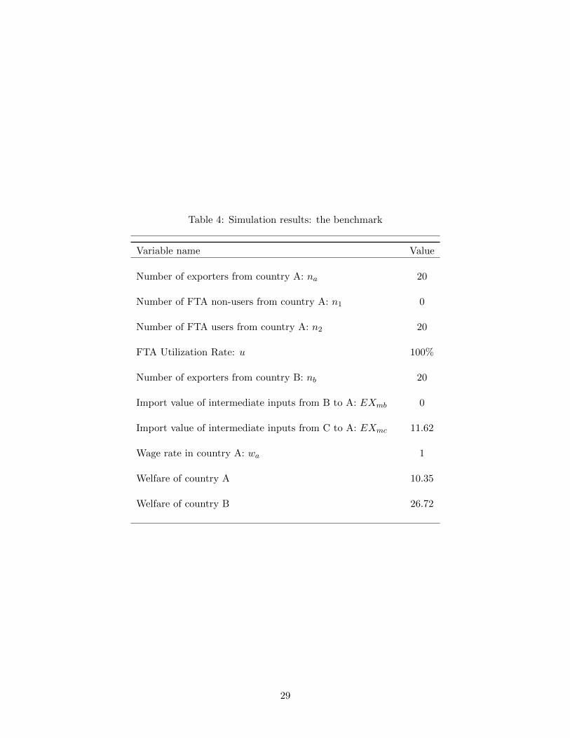
Table 4: Simulation results: the benchmark

Variable name Value

Number of exporters from country A: na 20

Number of FTA non-users from country A: n1 0

Number of FTA users from country A: n2 20

FTA Utilization Rate: u 100%

Number of exporters from country B: nb 20

Import value of intermediate inputs from B to A: EXmb 0

Import value of intermediate inputs from C to A: EXmc 11.62

Wage rate in country A: wa 1

Welfare of country A 10.35

Welfare of country B 26.72

29

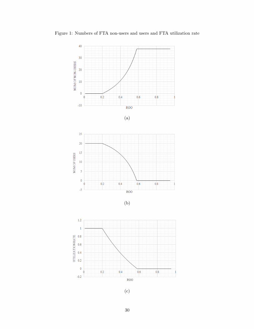
Figure 1: Numbers of FTA non-users and users and FTA utilization rate

(a)

(b)

(c)

30

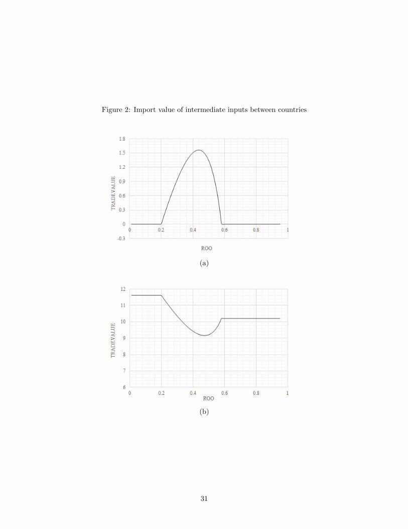
Figure 2: Import value of intermediate inputs between countries

(a)

(b)

31

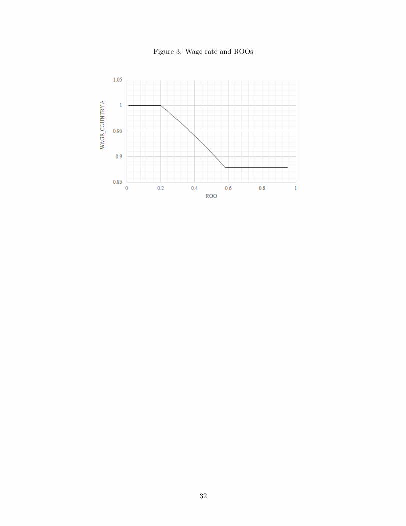
Figure 3: Wage rate and ROOs

32

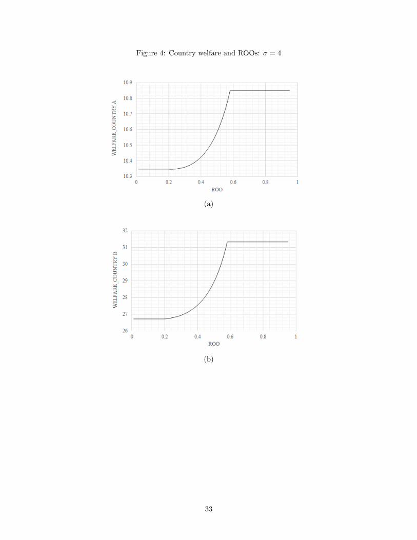
Figure 4: Country welfare and ROOs: σ = 4

(a)

(b)

33

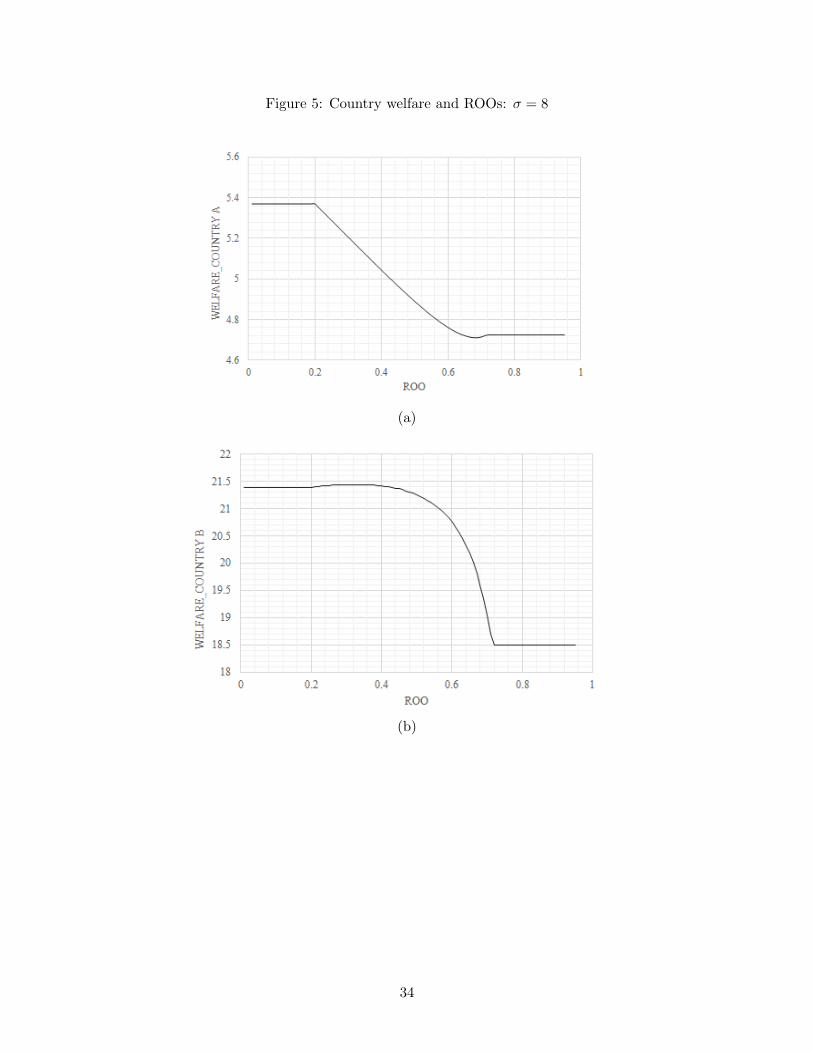
Figure 5: Country welfare and ROOs: σ = 8

(a)

(b)

34