1

A Work Project, presented as part of the requirements for the Award of a

Masters Degree in Economics from the Nova – School of Business and Economics

Effects of Quantitative Easing on the USA Economy:

A Test for Policy Effectiveness

Alexandre Marques Correia da Silva

630

Supervision of:

Luís Catela Nunes and Miguel Lebre de Freitas

June 2015

2

Effects of Quantitative Easing on the USA Economy:

A Test for Policy Effectiveness

Abstract

The catastrophic disruption in the USA financial system in the wake of the financial

crisis prompted the Federal Reserve to launch a Quantitative Easing (QE) programme in

late 2008. In line with Pesaran and Smith (2014), I use a policy effectiveness test to

assess whether this massive asset purchase programme was effective in stimulating the

economic activity in the USA. Specifically, I employ an Autoregressive Distributed Lag

Model (ARDL), in order to obtain a counterfactual for the USA real GDP growth rate.

Using data from 1983Q1 to 2009Q4, the results show that the beneficial effects of QE

appear to be weak and rather short-lived. The null hypothesis of policy ineffectiveness

is not rejected, which suggests that QE did not have a meaningful impact on output

growth.

Keywords: Counterfactual, Policy Effectiveness, Quantitative Easing, Zero Lower

Bound

Acknowledgments

I am grateful for the comments made by my advisors, Luis Catela Nunes and Miguel

Lebre de Freitas. I am very grateful for the invaluable support provided by Luis Filipe

Martins throughout the project. I would also like to thank the support provided by Ron

Smith and M. Hashem Pesaran.

3

1 Introduction

The 2008 financial turmoil prompted the Federal Reserve (Fed) to slash the federal

funds rate to extreme low levels. Deprived of its conventional monetary policy tool, the

Fed decided to embark on a series of unprecedented monetary policy actions, including

forward guidance and massive asset purchases, in order to restore stability in financial

markets and steer the economy. An extensive literature (Baumesteir and Benati (2010),

Chung et al. (2011), among others) has tried to gauge the extent to which the first round

of Quantitative Easing (QE1) unveiled in late 2008 promoted the recovery of the USA

economy. The broad consensus is that the large stimulus package implemented by the

Fed was successful in avoiding a depression in the USA.

Several other economies around the world have implemented nonstandard policy

measures amid concerns that near zero interest rates, the so-called Zero Lower Bound

(ZLB), would not be sufficient to spark recovery. In this study I pay particular attention

to the different unconventional monetary policy actions taken by the Fed and the

European Central Bank (ECB) in the wake of the crisis so as to establish possible links

between the monetary policies of the two central banks.

The ultimate goal of this study is to further explore the role played by QE1 in the

recovery of the USA economy by using a policy effectiveness test. In line with Pesaran

and Smith (2014), I use two Autoregressive Distributed Lag Models (ARDL), one that

covers the period before the announcement of the large scale asset purchases (1983Q1 –

2008Q4) and another that takes into account the full sample, from 1983Q1 to 2009Q4.

A policy intervention is given by a change in at least one of the policy parameters. The

null hypothesis of the policy effectiveness test is that the intervention is ineffective, that

is, there is no change in the policy parameters. Moreover, I aim to capture possible

4

indirect effects of the unconventional monetary policy actions implemented in Europe

on the USA economic activity by including in the model the real output growth rate of

the Euro Area.

The main conclusion of the study is that the beneficial effects of QE1 on output growth

were rather short-lived. This result is corroborated by the policy effectiveness test,

which indicates that the stimulus programme was ineffective in significantly boosting

the economic activity. As a result, one can argue that the actual improvement in the real

GDP growth rate in 2009 might have been due to other policies in place such as the

American Recovery and Reinvestment Act.

The rest of the paper is organized as follows: Section 2 describes the unconventional

monetary policy actions taken by the ECB and the Fed in the aftermath of the 2008

financial crisis, focusing however on the question of QE. Section 3 presents key

findings in the literature on the effects of large scale asset purchases at the ZLB. Section

4 discusses the methodology that was used in the empirical analysis. The results are

provided in Section 5. Finally, section 6 concludes.

2 Actions taken by the ECB and the Fed in the aftermath of

the crisis

The unconventional measures taken by the ECB and the Fed in response to the 2008

financial turmoil were significantly different, though with a common goal of improving

market functioning. However, it is not appropriate to make a comparison between those

different responses without taking into account the mandate and the institutional set-up

surrounding each central bank (Draghi, 2013). The primary mandate of the ECB is to

5

maintain price stability over the medium-long term, whereas that of the Fed

encompasses not only a price stability goal but also the promotion of maximum

employment and moderate long term interest rates. Moreover, unlike the Fed, the Treaty

on the Functioning of the European Union prohibits the ECB from purchasing

government debt in the primary market. Despite being a controversial issue, secondary-

market purchases of public debt by the ECB may be allowed as long as the main

objectives of the monetary financing condition are fulfilled, namely safeguarding the

primary aim of price stability and the independence of the central bank (ECB October

Bulletin, 2012).

The intervention of central banks in the bond markets is always a topic of intense

discussion as some economists believe that it might call into question the reputation,

and ultimately, the independence of the institution. However, when an interest rate is at

ZLB and the traditional monetary policy transmission mechanism is impaired, buying

government bonds might be the only credible solution to avoid persistent deflationary

pressures (Posen, 2010). Against this background, purchasing government bonds might

even enhance the credibility of the central bank.

Lenza et al. (2010) state that the financial structure in which each central bank operates

as well as the pre-crisis operational framework were two of the most important factors

behind the different responses of the Fed and the ECB to the crisis. To the extent that

banks play the predominant role in the provision of credit in Europe, the ECB

implemented unconventional measures aimed at increasing the liquidity of the banking

system, one of which was the increase in the maturity of the Eurosystem long-term

operations. These measures, coupled with a decrease in the short-term interest rate,

proved effective in ensuring the transmission of monetary policy, namely by

significantly reducing the interest rate charged on the small-loans to non-financial

6

corporations and households; by expanding the households´ volume of credit and

easing banks´ credit standards (ECB October Bulletin, 2010). In the USA, the Fed

launched a large-scale asset purchase programme – commonly referred to as

Quantitative Easing (QE) - with the purpose of tackling the huge disruption in capital

markets, on which non-financial corporations relied heavily to obtain credit. This

decision was made based on the conviction that just decreasing the Fed funds rate

would not be effective in restoring stability. The huge securitization in the American

financial system has been referred to as one of the reasons for the recent weaker impacts

of changes in the policy interest rate on the economy (Estrella (2002); Boivin et al.,

(2010)).

When it comes to the pre-crisis operational framework, the larger size of the

Eurosystem balance sheet when compared with that of the Fed implied that the demand

for extra liquidity was proportionally smaller in Europe (Lenza et al. (2010)).

Furthermore, a very limited set of assets were eligible as collateral by the Fed prior to

the crisis (mostly US treasury securities) whereas the ECB accepted a broad range of

assets, from corporate bonds to asset-backed securities. The narrower set of the eligible

collateral and the nefarious effects of the financial turmoil on the USA capital markets

prompted the Fed to have a much stronger reaction (in terms of balance sheet) to the

crisis than that of the ECB (Kohn, 2010).

In fact, the effects of the financial crisis on the economic activity were particularly acute

in the USA. A surge in the unemployment rate, the collapse of the Housing and Asset-

backed securities markets, and the tight restrictions on credit pushed down business and

consumer confidence1. Fischer (2013) argues that the countries where there was a

turmoil in the financial sector in the aftermath of the crisis were those that suffered a

1 This analysis is based on the Monetary Policy Report to the Congress, February 2009

7

stronger economic downturn. The absence of an alarming bubble in the Housing market

as well as the government support to banks watered down the effects of the catastrophe

on the European Economy.

The persistent low levels of inflation across the Eurozone in 2014 pushed the Governing

Council of the ECB into discussing the possibility of implementing a QE programme

(Draghi, 2014). The general view was that a prolonged period of extreme low levels of

inflation could trigger a dangerous process of de-anchoring of inflation expectations,

which in turn, with the nominal interest rate at the ZLB, could lead to an increase in the

real interest rate. The fear of lower inflation expectations mainly reflected the slowdown

in the economic activity of the Euro Area as a whole as well as the sharp downturn in

the oil market.

Quantitative Easing has been used by the major central banks in an environment of near

zero interest rates and gloomy outlook for inflation and economic activity. However, the

extent to which this massive injection of liquidity causes a rapid and sustainable

improvement in the economy is a contentious question. One of the traditional channels

through which QE affects the economic activity is the Portfolio Rebalancing Channel.

Joyce et al (2012) argues that a purchase of long-term government bonds – which on its

own tends to push the bonds yields down - tends to reduce the risk premium required by

investors to allocate their money to other long-term assets2, particularly corporate bonds

and equities. A growing body of literature, such as D`Amico and King (2010), Gagnon

et al. (2011) and Krishnamurthy and Jorgenson (2011), has indeed identified a negative

effect of QE on long term government bonds yields3 (see section 3). Lower yields might

2 This channel relies on the assumption that there is an imperfect substitutability of assets 3 Schenkelberg, Watzka (2011) state that, despite the broad consensus about the negative effect of QE on government bonds yields, investors might require a higher yield in case they perceive that the stimulus package will be successful in boosting inflation in the future.

8

induce governments to issue more debt in an attempt to refinance their liabilities at

lower interest rates, thereby countering the desired central bank´s change in the relative

supply of securities. Thus, the way this channel affects the real economy might hinge

on a potential coordination between the government´s debt-management policies and

the central banks´ actions (Bernanke and Reinhart (2004). This aspect is of paramount

importance when we compare the policies adopted by the ECB and the Fed. While in

the USA the fiscal implications of QE are possible to be dealt between the Treasury and

the central bank4, in Europe this coordination is virtually impossible to occur as there is

no European Treasury, but rather 18 different governments, each of which with its own

legislation.

3 Empirical evidence of the effects of QE at the ZLB

3.1 Inflation and Output growth

A growing literature has tried to assess the effects of asset purchase programmes on the

real economy when the short-term interest rate is constrained by the ZLB. Though a

consensus has not been reached yet, there is large evidence that unconventional

monetary policy was successful in avoiding a repeat of the Great Depression in the USA

(e.g Baumeister and Benati (2010), Chung et al. (2011) and Chen et al. (2012)). Using a

Bayesian VAR Sign Restrictions approach, Baumeister and Benati (2010) find that in

the absence of a compression in the yield spread the output growth in the USA would

have reached a trough of almost minus 10 percent in early 2009 and inflation would

4 Greenwood et al, (2014) provide data showing that the Fed´s attempts to reduce the supply of long-term bonds in capital markets in 2009 was partly offset by the Treasury´s decision to lengthen the average maturity of debt in order to alleviate fiscal risks associated with the rise in the government debt´s burden. The authors therefore call for new institutional arrangements aimed at promoting more cooperation between the two institutions.

9

have been negative. Chung et al. (2011) conclude that the combination of QE1 and QE2

boosted the real GDP growth in 3% and inflation in 1% when compared with the

scenario where the Fed would not have intervened. Based on a dynamic stochastic

general equilibrium model (DSGE), Chen et al. (2012) find that the second round of QE

adopted by the Fed expanded output growth by less than one third and inflation barely

changed relative to what would otherwise have happened in the absence of policy

intervention. Moreover, they show that the commitment to hold the fed funds rate at the

ZLB for an extended period of time tends to amplify the responses of inflation and

economic activity to large scale asset purchases.

Pesaran and Smith (2014) provide a test for policy effectiveness using reduced form

policy equations. As an illustrative test, they attempt to gauge the effectiveness of the

QE programme unveiled in March 2009 in the UK. Using an ARDL (1,1) model, they

conclude that a permanent 100 basis points reduction in the UK government spread has

an immediate positive impact on the real output growth rate, though it tends to be

temporary. Nevertheless, after applying a policy effectiveness test, they verify that the

null hypothesis is not rejected, which suggests that the Bank of England´s stimulus plan

was ineffective.

3.2 Bond markets

The Federal Reserve´s decision to embark on a massive purchase of medium-long term

assets came in two steps. In late November 2008, the Fed announced that it would

purchase agency mortgage-backed securities (MBS) and agency debt of up to 600

billion in order to avoid the collapse of these markets. The Fed decided to further

expand its balance sheet by announcing in March 2009 that it would purchase long-term

treasury securities.

10

0,0

1,0

2,0

3,0

4,0

5,0

6,0

20

08

Q1

20

08

Q2

20

08

Q3

20

08

Q4

20

09

Q1

20

09

Q2

20

09

Q3

20

09

Q4

20

10

Q1

20

10

Q2

Per

cen

tage

Moody BAA

yield -10

TCMR

10y - 2y

TCMR

10y TCMR

2y TCMR

Source : Federal Reserve Bank of ST.Louis (US)

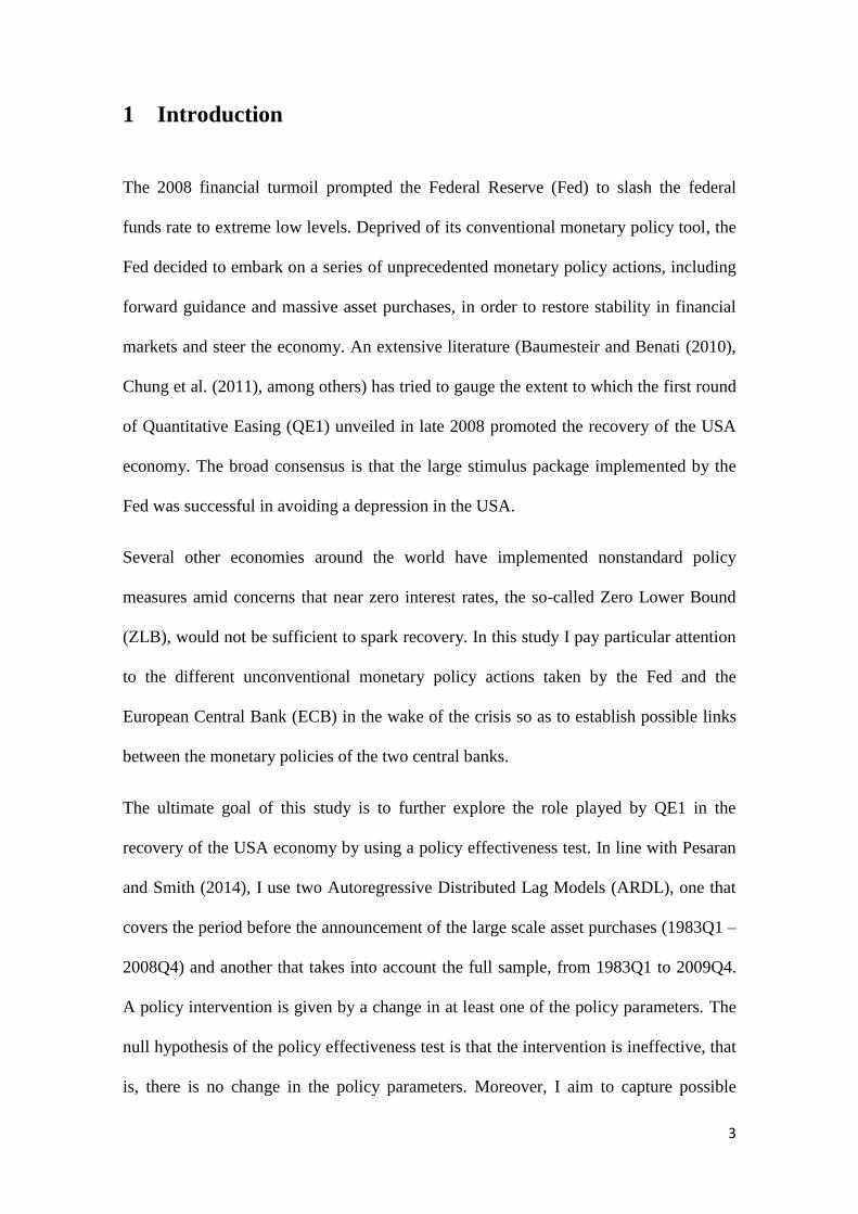
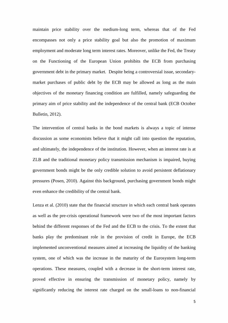
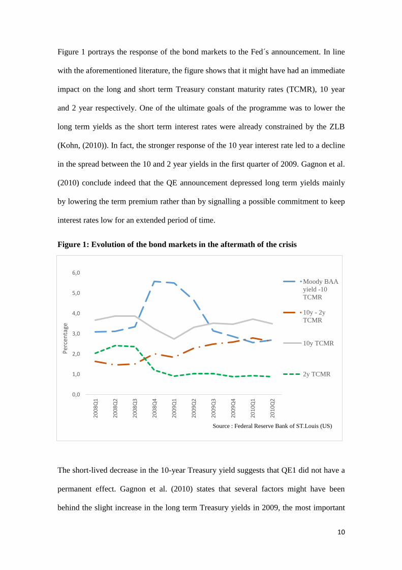
Figure 1 portrays the response of the bond markets to the Fed´s announcement. In line

with the aforementioned literature, the figure shows that it might have had an immediate

impact on the long and short term Treasury constant maturity rates (TCMR), 10 year

and 2 year respectively. One of the ultimate goals of the programme was to lower the

long term yields as the short term interest rates were already constrained by the ZLB

(Kohn, (2010)). In fact, the stronger response of the 10 year interest rate led to a decline

in the spread between the 10 and 2 year yields in the first quarter of 2009. Gagnon et al.

(2010) conclude indeed that the QE announcement depressed long term yields mainly

by lowering the term premium rather than by signalling a possible commitment to keep

interest rates low for an extended period of time.

Figure 1: Evolution of the bond markets in the aftermath of the crisis

The short-lived decrease in the 10-year Treasury yield suggests that QE1 did not have a

permanent effect. Gagnon et al. (2010) states that several factors might have been

behind the slight increase in the long term Treasury yields in 2009, the most important

11

of which were the improvement in the economic outlook and a strong reversal of the

flight-quality flows that had taken place after the break out of the crisis in 2008.

The notorious decline in the spread between the Moody Seasoned BAA corporate bond

yield and 10 year TCMR sheds light on the effects of the expansionary monetary policy

programme on the private borrowing costs. A decrease in the default and prepayment

risk premium are considered to be the main channels through which it negatively

affected BAA corporate bonds and mortgage backed-securities yields (Krishnamurthy

and Jorgensen, (2011)).

4 Methodology

In this section I briefly describe the model proposed by Pesaran and Smith5 (2014) that I

used in order to test for the effectiveness of QE1 in the USA.

Pesaran and Smith (2014) propose a macroeconometric rational expectations model and

they show that the reduced form is given by:

𝑞𝑡 = Φ (𝜃)𝑞𝑡−1 + 𝜓𝑥(𝜃)𝑥𝑡 + 𝜓𝑤 (𝜃)𝑤𝑡 + 𝜀𝑡 (1)

where 𝑞𝑡 is a vector that contains the endogenous variables, 𝑦𝑡 (the target variable) and

𝑧𝑡; 𝑥𝑡 is the policy exogenous variable and 𝑤𝑡 is a non-policy exogenous variable that is

assumed to be invariant to changes in 𝑥𝑡. 𝜃 is made up of a set of policy parameters, 𝜃𝑝,

and a set of structural parameters, 𝜃𝑠, that are assumed to be invariant to changes in the

former. A policy intervention is given by a change in at least one of the policy

parameters. The null hypothesis of the test is that the policy intervention is ineffective,

5 In this paper I only briefly expose the case of the dynamic model. Pesaran and Smith (2014) describe a model without dynamics as well.

12

that is, there is no evidence of change in 𝜃𝑝 after the intervention. 𝜀𝑡 accounts for

disturbances in the model. The policy intervention is assumed to occur at the end of

time t = 𝑇0 and as a result it is possible to have two different samples: one that covers

the pre-intervention period t = 𝑀,𝑀 + 1,… , 𝑇0 and another that is related to the post-

intervention period t = 𝑇0 + 1, 𝑇0 + 2,… , 𝑇0 + 𝐻. Thus, while the sample size of the

former is 𝑇 = 𝑇0 − 𝑀 + 1, the latter is equal to 𝐻.

The impact of the policy intervention on the target variable, 𝑦𝑡 , is given by the

difference between the realised outcomes,𝑦𝑇0+ℎ, and the counterfactual outcomes,

𝑦𝑇0+ℎ0 , during the post-intervention period,

𝑑𝑇0+ℎ = 𝑦𝑇0+ℎ − 𝑦𝑇0+ℎ0 , ℎ = 1,2,3, … ,𝐻 (2)

These estimated policy effects do not however accurately reflect the actual policy

impacts as the former will be subject to the post intervention random errors, 𝜀𝑦,𝑇0+ℎ .

Pesaran and Smith (2014) state that using a fully specified rational expectations

structural model might not give robust estimates of the counterfactual values once we

are uncertain about the specification of the complete model. As a result, they believe

that more accurate estimates of the counterfactual outcomes can be obtained by using

reduced form policy equations. After excluding the lagged values of 𝑧𝑡, they obtain an

ARDL model (𝑝𝑦, 𝑝𝑥, 𝑝𝑤) for pre and post-intervention samples :

𝑦𝑡 = ∑ 𝜆𝑖(𝜃0)𝑦𝑡−𝑖

𝑝𝑦

𝑖=1+ ∑ 𝜋𝑦𝑥,𝑖(𝜃

0)𝑥𝑡−𝑖 +𝑝𝑥𝑗=0 ∑ 𝜋𝑦𝑤,𝑖

′ (𝜃0)𝑤𝑡−𝑖 + 𝜐𝑦𝑡,𝑝𝑤𝑘=0 𝑡 = 𝑀,𝑀 +

1,𝑀 + 2,… , 𝑇0 (3)

𝑦𝑡 = ∑ 𝜆𝑖(𝜃1)𝑦𝑡−𝑖 + ∑ 𝜋𝑦𝑥,𝑖(𝜃

1)𝑥𝑡−𝑖 + ∑ 𝜋ý𝑤,𝑖′ (𝜃1)𝑤𝑡−𝑖

𝑝𝑤𝑘=0

𝑝𝑥𝑗=0

𝑝𝑦

𝑖=1+ 𝜐𝑦𝑡, 𝑡 = 𝑇0 +

1, 𝑇0 + 2,… , 𝑇0 + 𝐻 (4)

13

The reason for excluding the variable 𝑧𝑡 is that they aim to attribute to 𝑥𝑡 the possible

effects that the former might have on the target variable. In other words, they replace

the variable 𝑧𝑡 with its determinants, which are given by 𝑥𝑡.

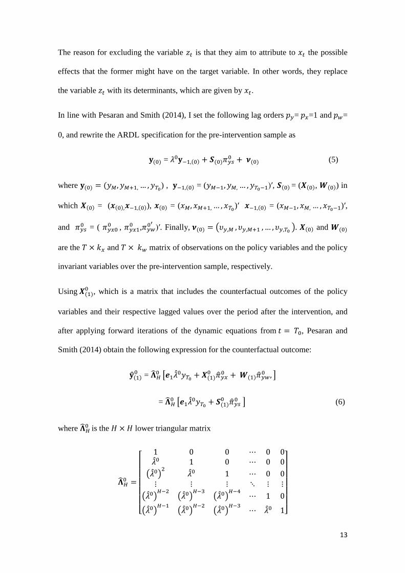
In line with Pesaran and Smith (2014), I set the following lag orders 𝑝𝑦= 𝑝𝑥=1 and 𝑝𝑤=

0, and rewrite the ARDL specification for the pre-intervention sample as

𝐲(0) = 𝜆0𝐲−1,(0) + 𝑺(0)𝜋𝑦𝑠0 + 𝝂(0) (5)

where 𝐲(0) = (𝑦𝑀, 𝑦𝑀+1, … , 𝑦𝑇0) , 𝐲−1,(0) = (𝑦𝑀−1, 𝑦𝑀, … , 𝑦𝑇0−1)′, 𝑺(0) = (𝑿(0), 𝑾(0)) in

which 𝑿(0) = (𝒙(0),𝒙−1,(0)), 𝒙(0) = (𝑥𝑀, 𝑥𝑀+1, … , 𝑥𝑇0)′ 𝒙−1,(0) = (𝑥𝑀−1, 𝑥𝑀, … , 𝑥𝑇0−1)′,

and 𝜋𝑦𝑠0 = ( 𝜋𝑦𝑥0

0 , 𝜋𝑦𝑥10 ,𝜋𝑦𝑤

0′)′. Finally, 𝝂(0) = (𝜐𝑦,𝑀 , 𝜐𝑦,𝑀+1 , … , 𝜐𝑦,𝑇0 ). 𝑿(0) and 𝑾(0)

are the 𝑇 × 𝑘𝑥 and 𝑇 × 𝑘𝑤 matrix of observations on the policy variables and the policy

invariant variables over the pre-intervention sample, respectively.

Using 𝑿(1)0 , which is a matrix that includes the counterfactual outcomes of the policy

variables and their respective lagged values over the period after the intervention, and

after applying forward iterations of the dynamic equations from 𝑡 = 𝑇0, Pesaran and

Smith (2014) obtain the following expression for the counterfactual outcome:

�̂�(1)0 = �̂�𝐻

0 [𝒆1�̂�0𝑦𝑇0

+ 𝑿(1)0 �̂�𝑦𝑥

0 + 𝑾(1)�̂�𝑦𝑤0 , ]

= �̂�𝐻 0 [𝒆1�̂�

0𝑦𝑇0+ 𝑺(1)

0 �̂�𝑦𝑠0 ] (6)

where �̂�𝐻 0 is the 𝐻 × 𝐻 lower triangular matrix

�̂�𝐻0 =

[

1 0 0 ⋯ 0 0�̂�0 1 0 ⋯ 0 0

(�̂�0)2

�̂�0 1 ⋯ 0 0

⋮ ⋮ ⋮ ⋱ ⋮ ⋮

(�̂�0)𝐻−2

(�̂�0)𝐻−3

(�̂�0)𝐻−4

⋯ 1 0

(�̂�0)𝐻−1

(�̂�0)𝐻−2

(�̂�0)𝐻−3

⋯ �̂�0 1]

14

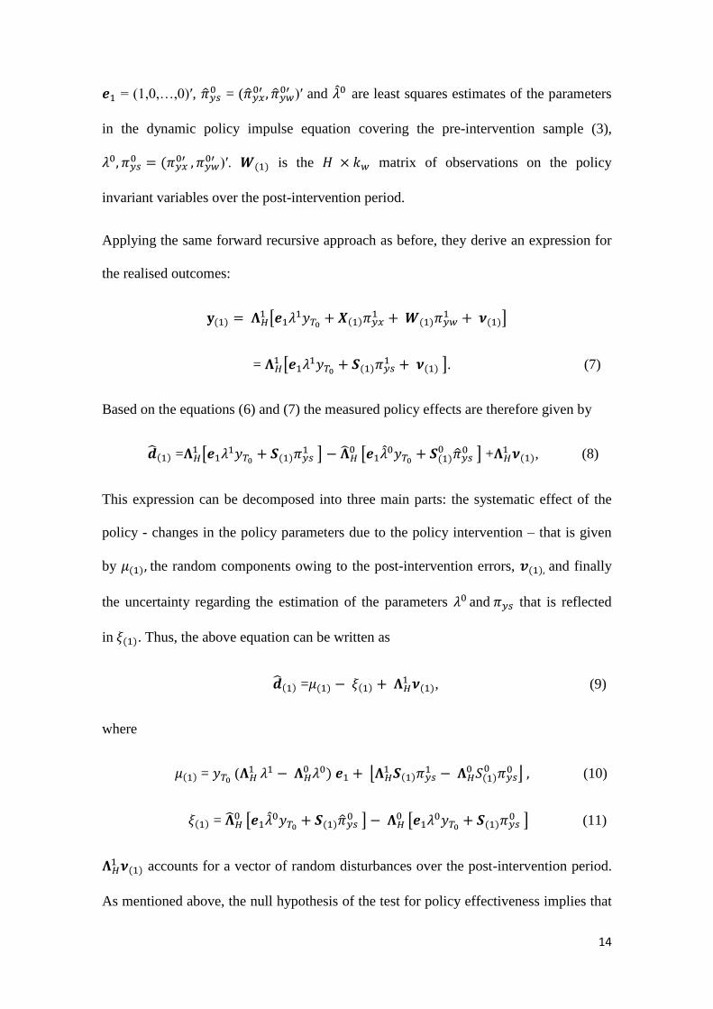
𝒆1 = (1,0,…,0)′, �̂�𝑦𝑠0 = (�̂�𝑦𝑥

0′ , �̂�𝑦𝑤0′ )′ and �̂�0 are least squares estimates of the parameters

in the dynamic policy impulse equation covering the pre-intervention sample (3),

𝜆0, 𝜋𝑦𝑠0 = (𝜋𝑦𝑥

0′ , 𝜋𝑦𝑤0′ )′. 𝑾(1) is the 𝐻 × 𝑘𝑤 matrix of observations on the policy

invariant variables over the post-intervention period.

Applying the same forward recursive approach as before, they derive an expression for

the realised outcomes:

𝐲(1) = 𝚲𝐻1 [𝒆1𝜆

1𝑦𝑇0+ 𝑿(1)𝜋𝑦𝑥

1 + 𝑾(1)𝜋𝑦𝑤1 + 𝝂(1)]

= 𝚲𝐻1 [𝒆1𝜆

1𝑦𝑇0+ 𝑺(1)𝜋𝑦𝑠

1 + 𝝂(1) ]. (7)

Based on the equations (6) and (7) the measured policy effects are therefore given by

�̂�(1) =𝚲𝐻1 [𝒆1𝜆

1𝑦𝑇0+ 𝑺(1)𝜋𝑦𝑠

1 ] − �̂�𝐻 0 [𝒆1�̂�

0𝑦𝑇0+ 𝑺(1)

0 �̂�𝑦𝑠0 ] +𝚲𝐻

1 𝝂(1), (8)

This expression can be decomposed into three main parts: the systematic effect of the

policy - changes in the policy parameters due to the policy intervention – that is given

by 𝜇(1), the random components owing to the post-intervention errors, 𝒗(1), and finally

the uncertainty regarding the estimation of the parameters 𝜆0 and 𝜋𝑦𝑠 that is reflected

in 𝜉(1). Thus, the above equation can be written as

�̂�(1) =𝜇(1) − 𝜉(1) + 𝚲𝐻1 𝝂(1), (9)

where

𝜇(1) = 𝑦𝑇0 (𝚲𝐻

1 𝜆1 − 𝚲𝐻0 𝜆0) 𝒆1 + ⌊𝚲𝐻

1 𝑺(1)𝜋𝑦𝑠1 − 𝚲𝐻

0 𝑆(1)0 𝜋𝑦𝑠

0 ⌋ , (10)

𝜉(1) = �̂�𝐻 0 [𝒆1�̂�

0𝑦𝑇0+ 𝑺(1)�̂�𝑦𝑠

0 ] − 𝚲𝐻 0 [𝒆1𝜆

0𝑦𝑇0+ 𝑺(1)𝜋𝑦𝑠

0 ] (11)

𝚲𝐻1 𝝂(1) accounts for a vector of random disturbances over the post-intervention period.

As mentioned above, the null hypothesis of the test for policy effectiveness implies that

15

there is an absence of change in the policy parameters after the intervention has taken

place, which means that the term 𝜇(1) has to be equal to zero. Moreover, Pesaran and

Smith (2014) state that in the dynamic case it is also necessary to assume that under 𝐻0

the reaction of the target variable to its lagged value is the same in the pre and post-

intervention period, that is 𝜆1 = 𝜆0, as well as 𝜐𝑦𝑡 is serially uncorrelated with a

constant variance, given by 𝜎𝜐2.

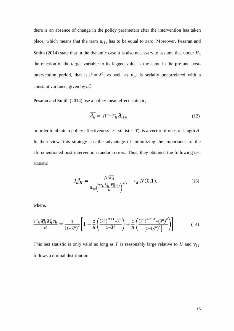
Pesaran and Smith (2014) use a policy mean effect statistic,

�̂�𝐻̅̅̅̅ = 𝐻−1 𝒯𝐻

′ �̂�(1), (12)

in order to obtain a policy effectiveness test statistic. 𝒯𝐻 ′ is a vector of ones of length 𝐻.

In their view, this strategy has the advantage of minimizing the importance of the

aforementioned post-intervention random errors. Thus, they obtained the following test

statistic

𝒯𝑑,𝐻𝑎 =

√𝐻𝑑�̂�̅̅ ̅̅

�̂�0𝑣(𝒯′𝐻�̂�𝐻

0 �̂�𝐻 0′𝒯𝐻

𝐻)

1/2 ⟶𝑑 𝑁(0,1), (13)

where,

𝒯′𝐻�̂�𝐻

0 �̂�𝐻 0′

𝒯𝐻

𝐻=

1

(1−�̂�0)2 [1 −

2

𝐻(

(�̂�0)𝐻+1

−�̂�0

1−�̂�0 ) +1

𝐻(

(�̂�0)2𝐻+2

−(�̂�0)2

[1−(�̂�0)2]

)] (14)

This test statistic is only valid as long as 𝑇 is reasonably large relative to 𝐻 and 𝝂(1)

follows a normal distribution.

16

5. Empirical Analysis

5.1Data

I use an ARDL model to estimate the effects of QE1 on the USA real output growth

rate, 𝑦𝑡. The full sample period (quarterly frequency) is from 1983Q1 to 2009Q4. The

growth rate is measured by the quarterly change in the logarithm of real GDP. Thus, I

extracted the quarterly seasonally adjusted series for real GDP from the St.Louis Fed´s

database. Following Pesaran and Smith (2014) I use the Euro Area real GDP growth

rate as a conditioning variable (𝑤𝑡) so as to capture possible indirect effects of the Euro

Area unconventional monetary policy actions on the USA output growth. This variable

is extracted from the Global VAR data set and includes eight countries, namely Austria,

Belgium, Finland, France, Germany, Italy, Netherlands, and Spain. The correlation

between the USA and Euro Area real output growth over the pre-intervention period

(1983Q1-2008Q4) is 0.37, lower than that observed over the full sample period, 0.47

(Figure A1 in the appendix). This large gap therefore suggests that the correlation

between the two growth rates intensified in the wake of the crisis.

As far as the policy variable is concerned, 𝑥𝑡, I use the quarterly seasonally unadjusted

spread between the 10 year and 2 Treasury Constant Maturity rate available in the

St.Louis Fed´s database. A few remarks are however needed to be made regarding this

choice. Firstly, the fact that the USA is one of the largest, if not the largest economy in

the world, could indicate that a change in the USA government bonds spread would

have a meaningful impact on the Euro Area output growth. Given the overwhelming

importance of the banking system in the dynamics of the European Economy (section

2), it is unreasonable to assume that such change would have sizeable effects on the

latter. Such view is corroborated by the correlation between the spread and the Euro

17

Area output growth, -0.47 and -0.46 over the pre-intervention period and full sample,

respectively. Secondly, the strong dependence of the USA economy on capital markets

prompted the use of a variable that could somehow reflect the reaction of these markets

to the large scale asset purchase programme. Gagnon et al. (2010) concluded that the

10-year term premium decreased between 38 and 82 basis points as a result of the Fed´s

$1.725 trillion asset purchases. Thus, for illustrative purposes, I regard the

counterfactual as the effect on the USA real GDP growth rate of there not having been a

60 basis points reduction - the average of Gagnon et al. (2010) ´s estimates6 - in the 10-

year government bond yield spread for the whole 2009.

5.2 Results

As the Schwarz criterion indicated one lag, the ARDL model that I consider is given by:

𝑦𝑡 = 𝜆𝑦𝑡−1 + 𝜋𝑦𝑥0𝑥𝑡 + 𝜋𝑦𝑥1𝑥𝑡−1 + 𝜋𝑦𝑤𝑤𝑡 + 𝜐𝑦𝑡 (14)

I consider two samples, one that covers the pre-intervention period (1983Q1 to 2008Q4)

and other that ends estimation in 2009Q4. Pesaran and Timmermann (2005) prove that

when our goal is to minimize out-of-sample mean squared forecast error, it may be

advantageous to include data before the intervention period to estimate forecasting

models on data samples that are subject to structural breaks. They state that this

preposition is only valid as long as some conditions are verified, including the fact that

the error variances should rise at the point of the structural break and the number of

observations in the post-intervention period, 𝐻, must be sufficiently low. To the extent

6 Baumeister and Benati (2010) also consider the average of Gagnon et al.´s (2010) time-series estimates

18

that the error variances increased in late 2008 and 𝐻 is equal to 4 - fulfilling in turn the

two conditions -, I followed the strategy proposed by Pesaran and Timmermann (2005).

For both sample periods, the equation above passes tests for serial correlation,

heteroskedasticity and normality, but it fails tests for functional form (at 1% level), that

is, there is evidence that the model is badly specified. The restriction that the long run

cumulative effect is equal to zero - 𝜋𝑦𝑥0 + 𝜋𝑦𝑥1 =0 – is not rejected (at 5% level) either

taking into account the pre-intervention sample or the full sample. The fact that the long

run effect is equal to zero is in line with standard macroeconomic theory that establishes

a temporary link between the rate of monetary growth and real output growth. Thus, this

restriction requires the use of the variation of spread, ∆𝑥𝑡, as a regressor in my model.

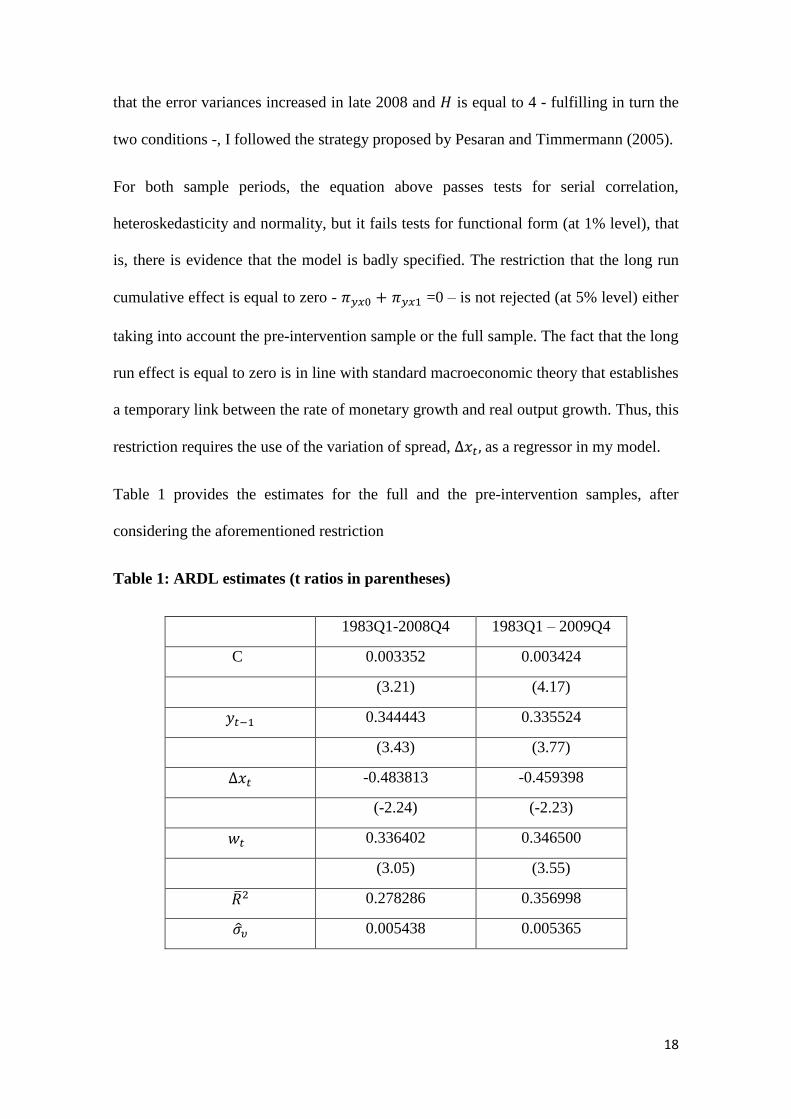
Table 1 provides the estimates for the full and the pre-intervention samples, after

considering the aforementioned restriction

Table 1: ARDL estimates (t ratios in parentheses)

1983Q1-2008Q4 1983Q1 – 2009Q4

C 0.003352 0.003424

(3.21) (4.17)

𝑦𝑡−1 0.344443 0.335524

(3.43) (3.77)

Δ𝑥𝑡 -0.483813 -0.459398

(-2.24) (-2.23)

𝑤𝑡 0.336402 0.346500

(3.05) (3.55)

�̅�2 0.278286 0.356998

�̂�𝜐 0.005438 0.005365

19

-0,02

-0,015

-0,01

-0,005

0

0,005

0,01

2009Q1 2009Q2 2009Q3 2009Q4

y_Realised y_Counterfactual Spread

The full-sample model suggests that a unit change in the variation of 10 year spread

would have a rather small impact effect, -0.46%. We can equally observe that a unit

change in the Euro Area output growth tends to increase the USA real GDP growth rate

by roughly 0.35%.

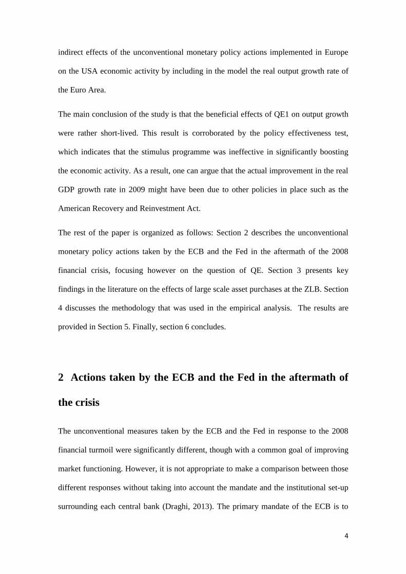
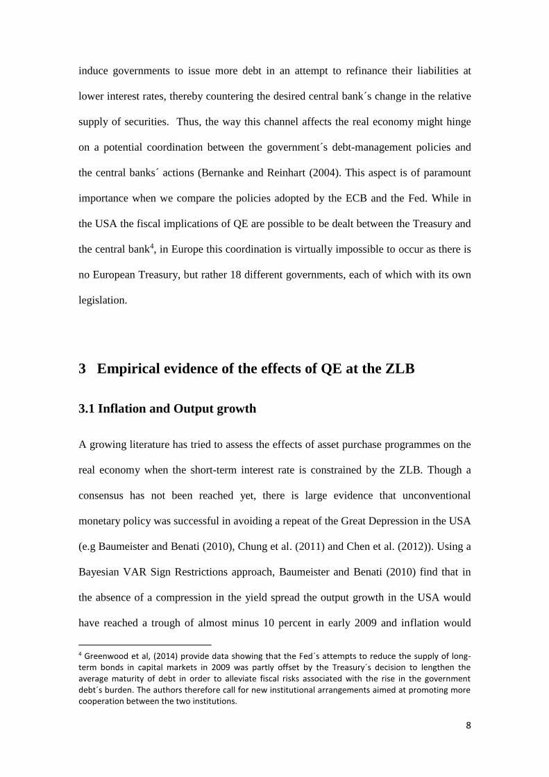
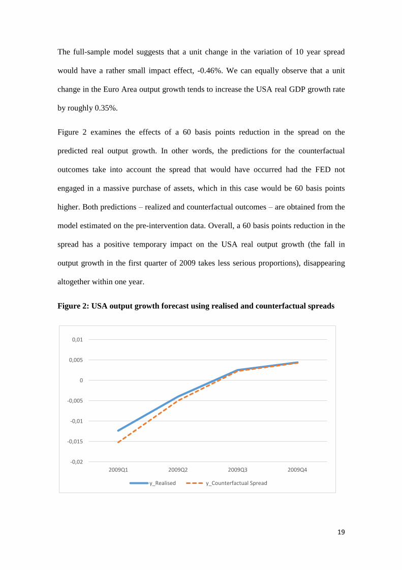
Figure 2 examines the effects of a 60 basis points reduction in the spread on the

predicted real output growth. In other words, the predictions for the counterfactual

outcomes take into account the spread that would have occurred had the FED not

engaged in a massive purchase of assets, which in this case would be 60 basis points

higher. Both predictions – realized and counterfactual outcomes – are obtained from the

model estimated on the pre-intervention data. Overall, a 60 basis points reduction in the

spread has a positive temporary impact on the USA real output growth (the fall in

output growth in the first quarter of 2009 takes less serious proportions), disappearing

altogether within one year.

Figure 2: USA output growth forecast using realised and counterfactual spreads

20

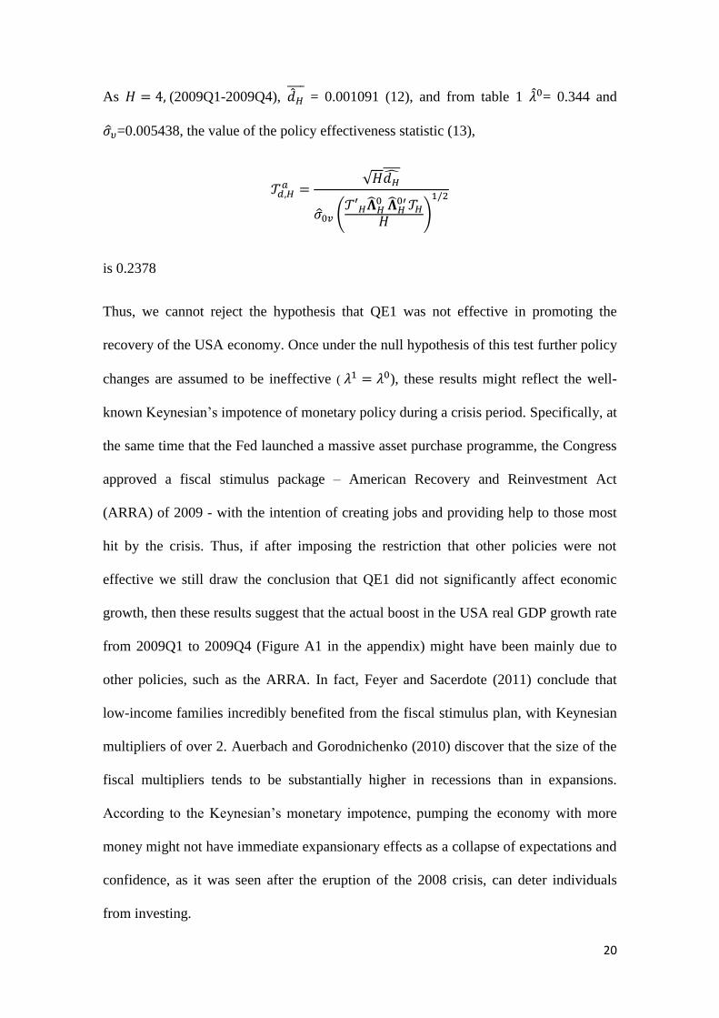
As 𝐻 = 4, (2009Q1-2009Q4), �̂�𝐻̅̅̅̅ = 0.001091 (12), and from table 1 �̂�0= 0.344 and

�̂�𝜐=0.005438, the value of the policy effectiveness statistic (13),

𝒯𝑑,𝐻𝑎 =

√𝐻𝑑�̂�̅̅̅̅

�̂�0𝑣 (𝒯′𝐻�̂�𝐻

0 �̂�𝐻 0′𝒯𝐻

𝐻 )

1/2

is 0.2378

Thus, we cannot reject the hypothesis that QE1 was not effective in promoting the

recovery of the USA economy. Once under the null hypothesis of this test further policy

changes are assumed to be ineffective ( 𝜆1 = 𝜆0), these results might reflect the well-

known Keynesian’s impotence of monetary policy during a crisis period. Specifically, at

the same time that the Fed launched a massive asset purchase programme, the Congress

approved a fiscal stimulus package – American Recovery and Reinvestment Act

(ARRA) of 2009 - with the intention of creating jobs and providing help to those most

hit by the crisis. Thus, if after imposing the restriction that other policies were not

effective we still draw the conclusion that QE1 did not significantly affect economic

growth, then these results suggest that the actual boost in the USA real GDP growth rate

from 2009Q1 to 2009Q4 (Figure A1 in the appendix) might have been mainly due to

other policies, such as the ARRA. In fact, Feyer and Sacerdote (2011) conclude that

low-income families incredibly benefited from the fiscal stimulus plan, with Keynesian

multipliers of over 2. Auerbach and Gorodnichenko (2010) discover that the size of the

fiscal multipliers tends to be substantially higher in recessions than in expansions.

According to the Keynesian’s monetary impotence, pumping the economy with more

money might not have immediate expansionary effects as a collapse of expectations and

confidence, as it was seen after the eruption of the 2008 crisis, can deter individuals

from investing.

21

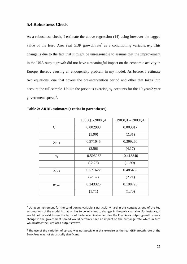
5.4 Robustness Check

As a robustness check, I estimate the above regression (14) using however the lagged

value of the Euro Area real GDP growth rate7 as a conditioning variable, 𝑤𝑡. This

change is due to the fact that it might be unreasonable to assume that the improvement

in the USA output growth did not have a meaningful impact on the economic activity in

Europe, thereby causing an endogeneity problem in my model. As before, I estimate

two equations, one that covers the pre-intervention period and other that takes into

account the full sample. Unlike the previous exercise, 𝑥𝑡 accounts for the 10 year/2 year

government spread8.

Table 2: ARDL estimates (t ratios in parentheses)

1983Q1-2008Q4 1983Q1 – 2009Q4

C 0.002988 0.003017

(1.90) (2.31)

𝑦𝑡−1 0.371045 0.399260

(3.56) (4.17)

𝑥𝑡 -0.506232 -0.418840

(-2.23) (-1.90)

𝑥𝑡−1 0.571622

0.485452

(-2.52) (2.21)

𝑤𝑡−1 0.243325 0.198726

(1.71) (1.70)

7 Using an instrument for the conditioning variable is particularly hard in this context as one of the key assumptions of the model is that 𝑤𝑡 has to be invariant to changes in the policy variable. For instance, it would not be valid to use the terms of trade as an instrument for the Euro Area output growth since a change in the government spread would certainly have an impact on the exchange rate which in turn would affect the Euro Area output growth. 8 The use of the variation of spread was not possible in this exercise as the real GDP growth rate of the Euro Area was not statistically significant.

22

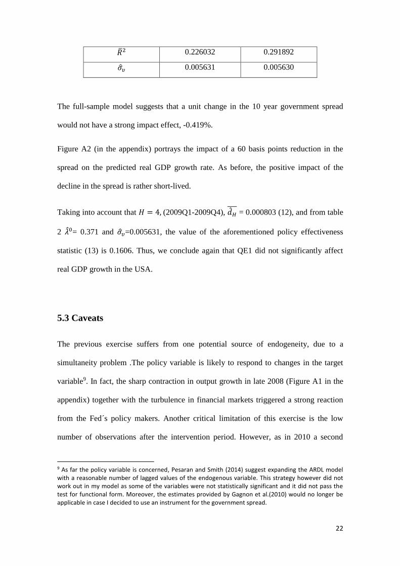
�̅�2 0.226032 0.291892

�̂�𝜐 0.005631 0.005630

The full-sample model suggests that a unit change in the 10 year government spread

would not have a strong impact effect, -0.419%.

Figure A2 (in the appendix) portrays the impact of a 60 basis points reduction in the

spread on the predicted real GDP growth rate. As before, the positive impact of the

decline in the spread is rather short-lived.

Taking into account that 𝐻 = 4, (2009Q1-2009Q4), �̂�𝐻̅̅̅̅ = 0.000803 (12), and from table

2 �̂�0= 0.371 and �̂�𝜐=0.005631, the value of the aforementioned policy effectiveness

statistic (13) is 0.1606. Thus, we conclude again that QE1 did not significantly affect

real GDP growth in the USA.

5.3 Caveats

The previous exercise suffers from one potential source of endogeneity, due to a

simultaneity problem .The policy variable is likely to respond to changes in the target

variable9. In fact, the sharp contraction in output growth in late 2008 (Figure A1 in the

appendix) together with the turbulence in financial markets triggered a strong reaction

from the Fed´s policy makers. Another critical limitation of this exercise is the low

number of observations after the intervention period. However, as in 2010 a second

9 As far the policy variable is concerned, Pesaran and Smith (2014) suggest expanding the ARDL model with a reasonable number of lagged values of the endogenous variable. This strategy however did not work out in my model as some of the variables were not statistically significant and it did not pass the test for functional form. Moreover, the estimates provided by Gagnon et al.(2010) would no longer be applicable in case I decided to use an instrument for the government spread.

23

round of asset purchases was adopted by the Fed, including observations after 2009

could seriously hamper the link that I was trying to establish between QE1 and the

recovery of the USA economy.

6 Conclusion

The aim of this paper is to assess the extent to which the Fed´s first round of QE

introduced in late 2008 was effective in stimulating the economic activity in the USA.

Based on the methodology proposed by Pesaran and Smith (2014) I have estimated two

ARDL models, one that ends estimation in 2008Q4 – before the announcement of the

programme – and another that covers the full sample (1983Q1 – 2009Q4). I have used

an ARDL (1,1) between the real output growth rate and the change in the spread

between the 10 year and 2 year treasury constant maturity rate, augmented by the Euro

Area real output growth. The fact that the real economy in the USA relies heavily on

credit provided by capital markets triggered the use of the government bonds spread as a

policy variable. The counterfactual simulations are obtained taking into account the

average of the estimates of Gagnon et al. (2010) regarding the effects of QE1 on the 10

year government spread. Specifically, I have assumed that the spread between the long

and short term interest rate would have been 60 basis points higher in the absence of the

policy intervention, for the whole 2009.

The model show that QE1 had an immediate positive impact on output growth, not

having however lasting effects. The policy effectiveness test supports this conclusion as

the null hypothesis of ineffectiveness is not rejected. Given the existence of potential

endogeneity problems in the original model, I have estimated two other equations using

the lagged value of the Euro Area real GDP growth rate as a conditioning variable. This

24

change does not appear to have had a significant impact on the results since the null

hypothesis of ineffectiveness keeps being not rejected. This conclusion suggests that

other policies might have played a stronger role in the recovery of the USA economy

such as the large fiscal economic plan, ARRA, approved by the Congress in 2009.

However, further research is needed to be done in order to accurately evaluate the role

played by the different policies.

REFERENCES

Auerbach, A. and Gorodnichencko, Y. 2012. “Measuring the Output Responses to

Fiscal Policy.” American Economic Journal; Economic Policy, Volume 4

Baumeister, C., and Benati, L. 2010. “Unconventional monetary policy and the great

recession – estimating the impact of a compression in the yield spread at the zero lower

bound.” Working paper series, No. 1258, European Central Bank.

Bernanke, B., and Reinhart, Vicent. 2004. “Conducting Monetary Policy at Very Low

Short-Term Interest Rates. “American Economic Review, Vol.94, 85-90.

Board of Governors of the Federal Reserve System. 2009. “Monetary Policy Report to

the Congress”, February, 1-36.

Boivin, J., Kiley, Michael. and Mishkin, F. 2010. “How Has the Monetary Transmission

Mechanism Evolved Over Time” Finance and Economics Discussion Series, 1-5, 22-

27.

D`Amico, S. and King, T. 2010 “Flow and Stock Effects of Large-Scale Treasury

Purchases” Finance and Economics Discussion Series

Draghi, M. 2013. “Introductory statement to the press conference (with Q&A)”, ECB, 2

May 2013.

Draghi, M. 2014 “Introductory Statement to the Press Conference (with Q&A)” ECB, 3

April 2014.

ECB. 2010. “The ECB´S Response to the Financial Crisis” Monthly Bulletin October

2010, European Central Bank.

ECB. 2012. “Compliance of Outright Monetary Transactions with the Prohibition of

Monetary Financing” Monthly Bulletin October 2012, 7-9, European Central Bank.

Estrella, Arturo.2002. “Securitization and the Efficacy of Monetary Policy” Economic

Policy Review, Volume 8, 1-5.

25

Gagnon, J., Raskin, M., Remache, J. and Sack, B. 2010. “Large-Scale Asset Purchases

by the Federal Reserve: Did They Work?” Federal Reserve Bank of New York, Staff

Reports.

Chen, H., Curdia, V. and Ferrero, A. 2012. “The Macroeconomic effects of Large-Scale

Asset Purchase Programs”, Working Paper Series, Federal Reserve Bank of San

Francisco.

Chung, H., Laforte, J., Reifschneider, D. and Williams, J. 2011. “Have we

Underestimated the Likelihood and Severity of Zero Lower Bound Events?” Working

Paper Series, Federal Reserve Bank of San Francisco.

Greenwood, R., Hanson, S., Rudolph, Joshua. and Summers, L. 2014. “Government

debt Management at the Zero Lower Bound” Hutchins Center Working Paper, No.5, 1-

7.

Feyer, J. and Sacerdote, B. 2011 “Did the Stimulus Stimulate? Real Time Estimates of

the Effects of the American Recovery and Reinvestment Act” Working Paper, No.

16759, National Bureau of Economic Research. 1-5, 22-25.

Joyce, M., Miles, D., Scott, A., and Vayanos. D. 2012. “Quantitative Easing and

Unconventional Monetary Policy – an Introduction” The Economic Journal, Volume

122, 271-288.

Krishnamurthy, A. and Vissing, J. 2011. “The Effects of Quantitative Easing on Interest

Rates”.

Kohn, D. 2010. “The Federal Reserve´s Policy Actions during the Financial Crisis and

Lessons for the Future” 1-4, 10-19.

Lenza, M., Pill, H., and Reichlin, L. 2010. “Monetary Policy in Exceptional Times”

Working Paper Series, No. 1253.

Pesaran, M., and Smith, R. 2014. “Counterfactual Analysis in Macroeconometrics: An

Empirical Investigation into the Effects of Quantitative Easing”.

Pesaran, M., and Timmermann, A. 2005. “Selection of Estimation Window in the

Presence of Breaks” 1-8.

Pill, H., Smets, F., and Fischer, S. 2013. “The Great Recession, Lessons for Central

Bankers” ed. Jacob Braude, Zvi Eckstein, Stanley Fischer and Karnit Flug, 2-4, 38-43.

Posen, A. 2010. “When Central Banks Buy Bonds Independence and the Power to say

No” Barclays Capital 14th Annual Global Inflation-linked conference, New York.

Schenkelberg, H., and Watzka. Sebastian. 2011. “Real effects of Quantitative Easing at

the Zero-Lower Bound: Structural VAR-based Evidence from Japan” CESifo, Working

Papers, No.3486.