doi: 10.1149/2.023301jes2013, Volume 160, Issue 1, Pages A15-A24.J. Electrochem. Soc. 

 Juhyun Song and Martin Z. Bazant Diffusion Impedance of Battery ElectrodesEffects of Nanoparticle Geometry and Size Distribution on

serviceEmail alerting

  click herein the box at the top right corner of the article or Receive free email alerts when new articles cite this article - sign up

http://jes.ecsdl.org/subscriptions go to: Journal of The Electrochemical SocietyTo subscribe to

© 2012 The Electrochemical Society

Journal of The Electrochemical Society, 160 (1) A15-A24 (2013) A150013-4651/2013/160(1)/A15/10/$28.00 © The Electrochemical Society

Effects of Nanoparticle Geometry and Size Distributionon Diffusion Impedance of Battery ElectrodesJuhyun Songa and Martin Z. Bazanta,b,∗,z

aDepartment of Chemical Engineering and bDepartment of Mathematics, Massachusetts Institute of Technology,Cambridge, Massachusetts 02139, USA

The short diffusion lengths in insertion battery nanoparticles render the capacitive behavior of bounded diffusion, which is rarelyobservable with conventional larger particles, now accessible to impedance measurements. Coupled with improved geometricalcharacterization, this presents an opportunity to measure solid diffusion more accurately than the traditional approach of fittingWarburg circuit elements, by properly taking into account the particle geometry and size distribution. We revisit bounded diffusionimpedance models and incorporate them into an overall impedance model for different electrode configurations. The theoreticalmodels are then applied to experimental data of a silicon nanowire electrode to show the effects of including the actual nanowiregeometry and radius distribution in interpreting the impedance data. From these results, we show that it is essential to account forthe particle shape and size distribution to correctly interpret impedance data for battery electrodes. Conversely, it is also possible tosolve the inverse problem and use the theoretical “impedance image” to infer the nanoparticle shape and/or size distribution, in somecases, more accurately than by direct image analysis. This capability could be useful, for example, in detecting battery degradationin situ by simple electrical measurements, without the need for any imaging.© 2012 The Electrochemical Society. [DOI: 10.1149/2.023301jes] All rights reserved.

Manuscript submitted May 21, 2012; revised manuscript received October 12, 2012. Published November 6, 2012.

In impedance spectra of intercalation battery electrodes, the re-sponse at low frequencies corresponds to solid-state transport ofcharge carriers (e.g. lithium ions and electrons in lithium ion batteries)in the active material. The transport of charge carriers is limited byionic diffusion in many battery materials due to the high mobility ofelectrons.1,2 For traditional battery electrodes with large particle sizes,the Warburg-type diffusion impedance, which draws a 45◦ line in thecomplex plane representation (Nyquist plot), has been widely reportedat low frequencies. Such response is well-described by a linearized dif-fusion model in a semi-infinite planar domain. This model leads to theoriginal Warburg impedance formula, ZW = AW (1 − i) ω−1/2, whereAW is the Warburg coefficient, i = √−1 is the unit imaginary num-ber, and ω is the radial frequency.3 With conventional particle sizesin micron scale or larger, the diffusion penetration depth from the ac-tive material/electrolyte interface does not effectively reach the centerof an intercalation particle in the typical frequency window (MHz∼ mHz) of an impedance measurement, and the original Warburgimpedance could be widely used in interpreting diffusion impedanceof battery electrodes.4

However, impedance spectra of modern thin film and nanoparti-cle battery electrodes show a distinguished feature in the diffusionimpedance: the response transitions from the original Warburg behav-ior to a capacitive behavior in a lower frequency range, represented bya vertical line in the complex plane representation.5–10 This transition isobserved because the diffusion penetration depth can reach the imper-meable current collector of a thin film electrode or the reflective centerof a nanoparticle at accessible low frequencies, due to short diffusionlengths in the thin film and nanoparticles. In the lower frequency range,the sinusoidal stimuli in impedance spectroscopy lead to effectivelyfilling up and emptying the active material, much like a capacitor, re-sulting in the vertical capacitive behavior. When diffusion impedancehas such behavior due to bounded diffusion space in active material,it is referred to as bounded diffusion (BD) impedance throughout thisarticle, while it has been called by various other names,2 such as open-circuit (blocked) diffusion,1 finite-space Warburg,4,11 and diffusionimpedance with impermeable12 or reflecting13 boundary conditions.

The BD impedance has different properties depending on electrodeconfiguration in terms of diffusion geometry and length distributionin active material. Ionic diffusivity and some of other electrochemicalparameters can be obtained from the diffusion impedance, providedthe configuration factors from modern electron microscopy and thefunctional formula from a mathematical model.14,15 While theoret-ical formulae of the BD impedance have been derived for a thin

∗Electrochemical Society Active Member.zE-mail: bazant@mit.edu

film electrode and nanoparticle electrodes with some model particlegeometries,2,6,12,13,16 they have not been widely applied by experimen-talists. In most applications, only the original Warburg impedancemodel and an one-dimensional BD impedance model have been ex-clusively used without considering the actual curved particle shapeand particle size distribution.7–10,17–19 Few studies employ models thatinvolve such configurational aspects in interpreting impedance.15,16,20

Likewise, only these two models are built into most commercial data-processing software products (e.g. Zview from Scribner Associates,Inc., ZSimpWin from EChem Software, and Echem Analyst fromGamry Instruments). As far as we know, MEISP+ from KumhoChemical Laboratories is the only product that involves BD impedancemodels for curved diffusion geometries.

In this article, we reformulate BD impedance models for planar,cylindrical, and spherical diffusion geometries and incorporate theminto an overall impedance model of battery electrodes, investigat-ing the effect of particle geometry and size distribution on diffusionimpedance. The models assume that the active material forms a solidsolution of intercalated ions, which has isotropic transport propertiesand high electron mobility. (Other factors affecting impedance, suchas phase separation, crystal anisotropy and charge separation, are be-yond the scope of this article, but are currently under investigationby our group.) In addition, for porous nanoparticle electrodes, it isassumed that the thickness of the electrode is thin and the electrolyteconductivity is high, so that the model does not account any gradientthat may develop along the electrode thickness. Various versions ofthe model were applied to experimental impedance data of a siliconnanowire electrode, which provides an ideal test case to study theeffects of including the actual nanowire geometry and radius distribu-tion in impedance models. Through this application, we show that it isessential to account for particle geometry as well as size distributionto accurately interpret impedance spectra of battery electrodes.

Theoretical Model

In impedance spectroscopy, a small sinusoidal stimulus either inpotential or current is applied about a reference state, and other vari-ables are perturbed accordingly. Each relevant variable can be writtenas a superimposition of two terms: a term describing the referencestate response in the absence of the perturbation, and another termdescribing the perturbation about the reference state. The small am-plitudes of the perturbations allow mathematical linearization of thesystem, and thus the perturbations in all relevant variables have a sinu-soidal form with an identical frequency. An arbitrary system variable,

A16 Journal of The Electrochemical Society, 160 (1) A15-A24 (2013)

X, can be expressed as

X = Xref + Re[Xeiωt ] [1]

where i is the unit imaginary number, ω is the radial frequency, and t isthe time variable. The former term, Xref , represents the reference stateresponse, and the latter term represents the sinusoidal perturbation inX with a complex exponential, eiωt , and the Fourier coefficient, X .The Fourier transformation of the perturbation yields X , which isa complex number containing information related to the magnitudeand the phase of the perturbation. X can be either current density, j ,potential, φ, or local concentration, c.

Bounded diffusion impedance.— The system under initial inves-tigation is a thin film or a single nanoparticle of active material, inwhich ions intercalate from its interface with electrolyte, and electronscome from its interface with a current collector or a conducting agent.We take an equilibrium reference state with uniform concentrationsof the charge carriers, restricting our model to materials that form asolid solution with the ions. In most active materials, the mobility ofelectrons is much higher than that of ions.2 As electrons become freelyavailable in the system, the mean electric field quickly relaxes, result-ing in local charge neutrality in the bulk.11,21 Under such conditionsionic diffusion limits transport of the charge carriers, and a neutraldiffusion equation, Fick’s law, can be recovered for the ion materialbalance in the system.22

∂c

∂t= Dch∇2c [2]

where c is the ion concentration, t is the time variable, and Dch isthe chemical diffusivity of ions in the active material. Impedancebehavior in a system with comparable electron and ion mobilities hasbeen studied by several groups.22–24

We hereby focus on model electrode configurations, including athin film electrode, and nanoparticle electrodes with planar, cylindri-cal, and spherical particles. Figure 1 shows the model electrode con-figurations and the corresponding solid-state diffusion geometries inthe active material. Under the assumption of isotropic transport prop-erties, the diffusion equation can be reduced to an ordinary differentialequation in frequency-space domain through Fourier transformation.

iωc = Dch∇2c = Dch

xn−1

d

dx

(xn−1 dc

dx

)[3]

x

x

(a) (b)

(c)

0l 0

l

l

(d)

x

0

l

x

0

Figure 1. Model electrode configurations, particle geometries, and corre-sponding coordinate systems, where the blue region and the gray region rep-resent the active material and the current collector, respectively: (a) thin filmelectrode, (b) electrode with planar particles, (c) electrode with cylindricalparticles, and (d) electrode with sphere particles.

where the spatial variable, x , is the distance from the current collectorin the thin film, or the distance from the center of symmetry in theplanar, cylindrical, and spherical nanoparticles (see Figure 1). Thederivative term accounts for variation in the x-normal area with respectto x , where n is the dimension number: 1 for a thin film electrodeand a planar nanoparticle, and 2 and 3 for cylindrical and sphericalnanoparticles, respectively.

One of the boundary conditions describes the impermeability ofions at the current collector of a thin film electrode or the symmetryat the center of a nanoparticle.

dc

dx

∣∣∣∣x=0

= 0 [4]

This impermeable or reflective boundary condition indicates that thediffusion space is bounded. The other boundary condition appliesFaraday’s law at the active material/electrolyte interface to correlatethe ion flux and the intercalation current density.

jintc = −eDchdc

dx

∣∣∣∣x=l

[5]

where jintc is the intercalation current density, e is the electron chargeconstant, and l is the film thickness in a thin film, a half of the thicknessin a planar nanoparticle, or the radius in a cylindrical and a sphericalnanoparticle. With these boundary conditions, the differential equationcan be integrated to give the perturbation profile of ion concentrationin the model geometries.

The contribution of solid-state diffusion in the active material ap-pears in an equilibrium potential of the intercalation reaction, since itis a function of the ion concentration at the surface where the reactiontakes place. Therefore, the definition of local diffusion impedancetakes a partial derivative of the equilibrium potential with respect toion concentration, and the perturbation in ion concentration at thesurface, in place of a potential perturbation.6,12,16

zD = �φeq

jintc

=(

∂�φeq

∂c

)c|x=l

jintc

[6]

where �φeq is the equilibrium potential of the intercalation reaction,and zD is the local diffusion impedance. This definition is applied toa system of bounded diffusion space to define local BD impedance.

Properties of the BD impedance can be well-studied when theequations are reduced to their dimensionless forms by proper scaling.The frequency can be scaled by the diffusion characteristic frequency,ωD = Dch/l2, that appears when non-dimensionalizing the diffusionequation.

ω = ω

ωD[7]

As the diffusion characteristic frequency is approached, the diffu-sion penetration depth reaches the impermeable current collector ofa thin film electrode or the symmetric center of a particle. The lo-cal BD impedance can be scaled by the BD impedance coefficient,ρD = (−∂�φeq/∂c)(l/eDch), which becomes its apparent scale whenEquations 5 and 6 are combined.

zD = zD

ρD[8]

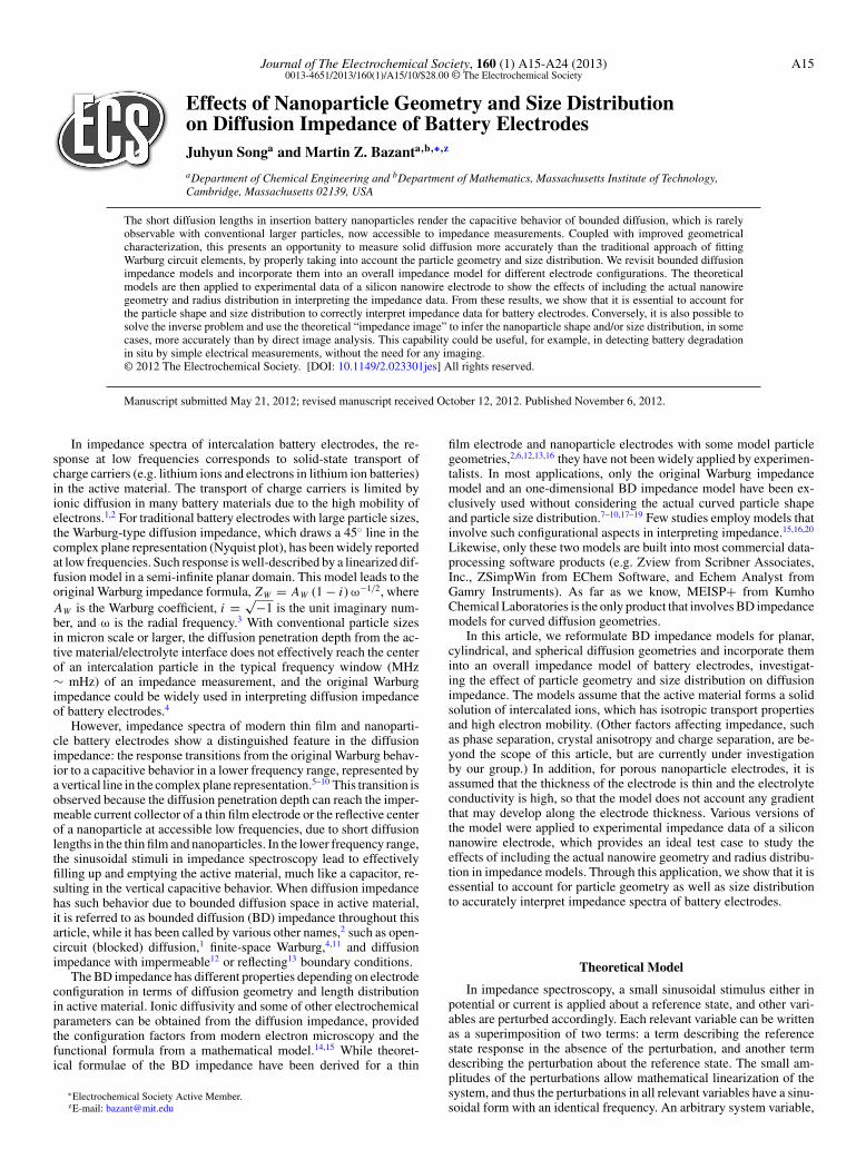
In Table I, dimensionless forms of the local BD impedance for themodel diffusion geometries are summarized with their asymptoticbehaviors, where I0 and I1 are the first kind modified Bessel functionsof zero and first order, respectively. zD∞ and zD0 are the asymptoticapproximations of zD at high and low frequencies, respectively.6,12,25

Local interface impedance.— We consider a simple interfacemodel of the active material in which the active material is in directcontact with the electrolyte solution without any additional resistivelayer, such as solid electrolyte interface (SEI) layer.16 Local elec-troactive processes on the active material/electrolyte interface includecharging of the double layer and intercalation of ions into the active

Journal of The Electrochemical Society, 160 (1) A15-A24 (2013) A17

Table I. Dimensionless local BD impedance and their asymptotic approximations for the model electrode configurations and particlegeometries.

Thin film electrode and planar particle (n = 1) Cylindrical particle (n = 2) Spherical particle (n = 3)

zDcoth

(√iω

)√

iω

I0

(√iω

)√

iωI1

(√iω

) tanh(√

iω)

√iω−tanh

(√iω

)

zD∞ (ω � 1) 1√2ω

(1 − i) 1√2ω

(1 − i) − 12ω

i 1√2ω

(1 − i) − 1ω

i

zD0 (ω 1) 13 − 1

ωi 1

4 − 2ω

i 15 − 3

ωi

material. The electrochemical double layer develops at the interfacedue to the potential drop across it. The double layer charging processcan be modeled with the ideal capacitor equation. Using Fourier-transformed variables, the current density becomes

jdl = iωqdl = iωCdl�φ [9]

where jdl is the double layer charging current density, qdl is the doublelayer charge density, Cdl is the double layer capacitance, and �φ isthe potential drop across the active material/electrolyte interface.

Another current contribution comes from intercalation of ions intothe active material. The intercalation kinetics can be modeled with theButler-Volmer equation which, in general, describes a charge transferreaction rate. The intercalation current density can then be written as

jintc = j0[exp

(α

eη

kT

)− exp

((α − 1)

eη

kT

)][10]

where α is the electron transfer symmetry factor (0 < α < 1), j0 is theexchange current density, and η = �φ − �φeq is the surface overpo-tential. Linearization of the Butler-Volmer equation should considerthat both j0 and �φeq fluctuate due to the perturbation in ion concen-tration at the active material surface. When the system is perturbedaround an equilibrium reference state, the two exponential terms eval-uated at the reference state cancel each other out, and thus the pertur-bation in j0 does not effectively contribute to the impedance response.On the other hand, the perturbation in �φeq brings the contributionfrom solid-state diffusion in the active material, and introduces thelocal diffusion impedance. Taking the Fourier transformation, the lin-earized Butler-Volmer equation becomes

jintc = j0e

kT

(�φ −

(∂�φeq

∂c

)c|x=l

)

= 1

ρct(�φ − zD jintc) [11]

where ρct = kT / j0e is the charge transfer resistance, and the definitionof local diffusion impedance was used. The equation can be rearrangedto give a generalized Ohm’s law, which leads to a circuit analog of theion intercalation process.

(ρct + zD) jintc = �φ [12]

This indicates that ion intercalation could be represented by a seriescircuit of ρct and zD , given a small perturbation.

We assume an independent parallel arrangement of the doublelayer charging current and the intercalation current on the active ma-terial/electrolyte surface, following Randle and Graham.26,27

jtot = jdl + jintc [13]

where jtot is the total current density. Using the total current densityand the potential drop at the interface, we can define local interfaceimpedance as

zint f = �φ

jtot

= (iωCdl + (ρct + zD)−1)−1 [14]

where zint f is the local interface impedance. The local interfaceimpedance can be represented by the Randle’s equivalent circuit,which has Cdl in parallel with a series of ρct and zD , as shown inFigure 2. As the model contains the parallel contribution of Cdl and

ρct , a resistive-capacitance (RC) characteristic frequency naturallyarises, ωRC = (ρct Cdl )

−1, around which relative magnitudes of jdl

and jintc are flipped.The local interface impedance can be scaled by ρct to give its

dimensionless form.

zint f = zint f

ρct=

(i (ωDρct Cdl ) ω +

(1 + ρD

ρctzD

)−1)−1

= (i(ω/ωRC/D) + (1 + ρD/ct zD)−1)−1 [15]

where ωRC/D = ωRC/ωD is the characteristic frequency ratio, andρD/ct = ρD/ρct is the dimensionless BD impedance coefficient. Thetwo dimensionless parameters, ωRC/D and ρD/ct , determine the be-havior of the local interface impedance. ωRC/D is a measure of theseparation of the two characteristic frequencies, ωRC and ωD . Formost battery electrodes, ωRC/D is a large number, and the local inter-face impedance leads to well-separated RC and BD elements in theoverall impedance spectra; the RC element ideally draws a semicircleat high frequencies with its summit at ωRC , and the BD element drawsa hockey-stick-like curve at low frequencies with its kink around ωD

in the complex plane representation. Relative magnitudes of the twoelements are determined by ρD/ct .

Overall impedance response.— While local impedance responsehas been considered to this point, impedance spectroscopy measuresthe integrative response of an entire electrode that may involve un-even local impedance response on its surface. Thus overall electrodeimpedance is defined with a total current which could be obtained byintegrating jtot over the entire electroactive surface. When a thin filmelectrode has a uniform thickness, jtot is even over the entire surfaceand the integration results in a trivial scaling of jtot by the total area.On the other hand, for porous nanoparticle electrodes, we assumethe conduction characteristic frequency in the electrolyte solution isconsiderably higher than ωD and ωRC ; that is, this overall impedancemodel does not account for potential and concentration gradient thatmay develop along the electrode thickness. This assumption is validwhen the conductivity of the electrolyte solution is high enough and/orwhen the thickness of a porous electrode is thin enough. Under suchcondition, it is the heterogeneity in particle size that leads to non-uniform jtot across particles in a nanoparticle electrode, while eachisotropic particle has even jtot on its surface. A particle size, which

Cdl

zD

Figure 2. Randle’s equivalent circuit, a circuit analogy of local interfaceimpedance, where Cdl is the double layer capacitance, ρct is the charge transferresistance, and zD is the local diffusion impedance.

A18 Journal of The Electrochemical Society, 160 (1) A15-A24 (2013)

is the solid-state diffusion length, l, in the diffusion model, is consid-ered as a realization of a continuous random variable with a certainprobability density function (PDF). The integration could then be per-formed with respect to l, in which jtot is weighted by a product ofparticle population and surface area.

J =∫

jtot (l) d A = Ntot

∫ ∞

0PrL (l) ap (l) jtot (l) dl [16]

where J is the total current, A is the electroactive surface area, Ntot

is the total number of particles, and PrL is the PDF of the solid-statediffusion length, a random variable, L . ap (l) is the average surface areaof a single particle with L = l; ap (l) is 2ax for planar particles, 2πHlfor cylindrical particles, and 4πl2 for spherical particles, respectively,where ax is the average sidewall area of the planar particles and H isthe average height of the cylindrical particles.

Also, an impedance measurement inevitably involves interferencesfrom cell connections as well as transports of ions in the electrolytephase, whose contribution could be modeled with a resistor in thetypical frequency window of an impedance measurement. Therefore,the overall impedance of a nanoparticle electrode can be written asfollows.

Z = Rext + �φ

J= Rext + �φ

Ntot

∫ ∞0 PrL (l) ap (l) jtot (l) dl

= Rext +(

Ntot

∫ ∞

0PrL (l) ap (l) z−1

int f (l) dl

)−1

[17]

where Rext is the external resistor that represents the contributionfrom cell connections and transports in electrolyte phase. While thismodel omits the gradient in potential and ion concentration alongthe electrode thickness, detailed elaboration regarding their effects onimpedance of a battery electrode can be found in references 15, 16,20.

When L has a narrow enough distribution, its PDF can be approx-imated by a Dirac delta function, which makes the integration trivial.This approximation is equivalent to assuming an identical particlesize in a nanoparticle electrode. Under such a condition, the overallimpedance becomes

Z = Rext+(

Ntot

∫ ∞

0δ(l−L

)ap (l) z−1

int f (l) dl

)−1

=Rext+zint f

(L)

Atot[18]

where δ is the Dirac delta function, L is the average solid-state diffu-sion length, and Atot is the total surface area. The overall impedanceof a uniform thin film electrode has the same expression, having one-dimensional BD impedance in zint f .

The overall impedance in Equation 17 can be reduced to its di-mensionless form, defining the dimensionless overall impedance,Z = Atot Z/ρct , and the dimensionless solid-state diffusion length,l = l/L , along with the dimensionless variables defined previ-ously. The frequency and the RC characteristic frequency are nowscaled by ωD(L) = Dch/L2, and their dimensionless forms becomeω = ω/ωD(L) and ωRC/D = ωRC/ωD(L). Expanding the local inter-face impedance, zint f , the overall impedance becomes

Z = Atot Z

ρct= Atot Rext

ρct+

(∫ ∞

0PrL (l) ˜a p(l)z−1

int f (l)dl

)−1

= Rext + (i(ω/ωRC/D) +∫ ∞

0PrL (l) ˜a p(l)(1 + ρD/ct (l)zD(l))−1dl)−1

[19]

Here, Rext = Atot Rext/ρct is the dimensionless external resistance,and it indicates the relative magnitude of the external resistance withrespect to the charge transfer resistance. PrL is the PDF of the dimen-sionless solid-state diffusion length, a random variable, L = L/L .When a lognormal PDF is used for PrL , it can be solely describedby the dimensionless standard deviation, σ, which is a measure of

10-3

10-1

101

103

10-2 10-1 1 101 102 103

45

60

75

90

0 0.2 0.4 0.6 0.8 10

0.2

0.4

0.6

0.8

1

1.2

1.4

planarcylindricalspherical

(a) (b)

(c)

10-2 104

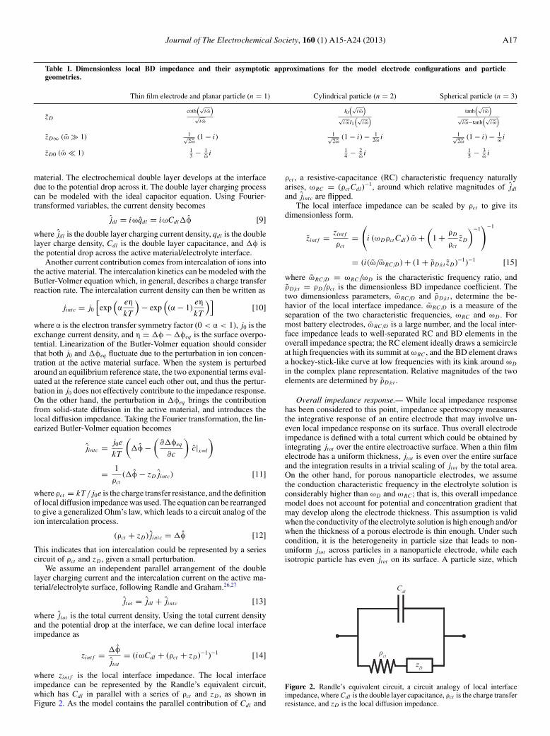
Figure 3. Dimensionless local BD impedance for different particle geome-tries: (a) complex plane plot, (b) magnitude plot, and (c) phase plot.

the heterogeneity in particle size. ˜a p(l) = ap(l)/ap(L) = l n−1 is thedimensionless average surface area of a single particle with L = l,and it gives different weighting distributions on the local impedancein the integral, depending on the particle geometry.

Results

Effect of nanoparticle geometry.— To isolate the effect of solid-state diffusion geometry on diffusion impedance, we first look at thelocal BD impedance, zD . Figure 3 shows zD for the model diffusiongeometries in various formats. For all the diffusion geometries, aclear transition is observed near ω ≈ 1, around which the diffusionpenetration depth reaches the impermeable current collector of a thinfilm electrode or the symmetric center of a particle. At ω � 1, aWarburg regime is defined, where zD asymptotically approaches theoriginal Warburg behavior in its high frequency limit. In this regime,the penetration depth is shorter than the diffusion length, l, and thebounded diffusion behaves much like semi-infinite diffusion. On theother hand, at ω 1, a capacitive regime is defined, where zD has acapacitive behavior, drawing a vertical line in the complex plane plotand approaching 90◦ in the phase plot. In this regime, the penetrationdepth exceeds l, and the perturbation leads to effectively filling up andemptying the active material, much like a capacitor.

In both regimes, zD has different behavior depending on diffusiongeometry, as denoted by its asymptotic approximations in high andlow frequencies, zD∞ and zD0, respectively. For the planar diffusiongeometry, zD∞ has the form of the original Warburg impedance, andzD follows the original Warburg behavior in most of the Warburgregime. On the other hand, for the curved diffusion geometries, thecylindrical and spherical models, zD∞ retains an extra imaginary termin addition to the original Warburg formula. This implies that forthe curved diffusion geometries, zD in the Warburg regime can beapproximated by a series circuit of the original Warburg impedanceand a capacitance, CD∞ = 2/(n − 1). Correspondingly in this regime,the zD curves have positive deviation in phase angle, or capacitivedeviation, from the original Warburg behavior. The deviation reflectsthe variation in the flux-normal area with respect to the distance fromthe active material/electrolyte interface; it is larger for the sphericalgeometry than for the cylindrical.

On the other hand, zD0 indicates that zD in the capacitive regimecan be analogized to a series circuit of a resistance, ρD0 = 1/(n + 2),and a capacitance, CD0 = 1/n, whose values differ for the differentdiffusion geometries. The differences in this regime arise primarilyfrom different aspect ratios of the model geometries. ρD0 is smallerfor the more-curved geometry; that is, it is smaller for the sphericalgeometry than for the cylindrical, and it is smaller for the cylindricalgeometry than for the planar geometry. This difference exists becauseit is easier to diffuse throughout the entire domain with a higher surfaceto volume ratio, given an identical diffusion length and driving force onthe surface. CD0 is also smaller for the more-curved geometry, becauseit has smaller volume to accommodate ions. Correspondingly, in the

Journal of The Electrochemical Society, 160 (1) A15-A24 (2013) A19

0 1 2 30

1

2

3

0 1 2 30

1

2

3

0 1 2 30

1

2

3

0 1 2 30

1

2

3

0 1 2 30

1

2

3

0 1 2 30

1

2

3

−Z

planarcylindricalspherical

= 0 = 0.25

= 0.5 = 0.75

= 1 = 1.5

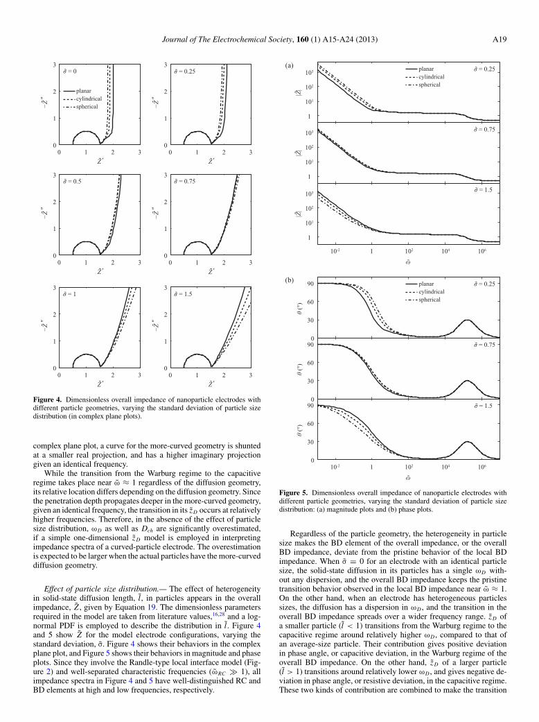
Figure 4. Dimensionless overall impedance of nanoparticle electrodes withdifferent particle geometries, varying the standard deviation of particle sizedistribution (in complex plane plots).

complex plane plot, a curve for the more-curved geometry is shuntedat a smaller real projection, and has a higher imaginary projectiongiven an identical frequency.

While the transition from the Warburg regime to the capacitiveregime takes place near ω ≈ 1 regardless of the diffusion geometry,its relative location differs depending on the diffusion geometry. Sincethe penetration depth propagates deeper in the more-curved geometry,given an identical frequency, the transition in its zD occurs at relativelyhigher frequencies. Therefore, in the absence of the effect of particlesize distribution, ωD as well as Dch are significantly overestimated,if a simple one-dimensional zD model is employed in interpretingimpedance spectra of a curved-particle electrode. The overestimationis expected to be larger when the actual particles have the more-curveddiffusion geometry.

Effect of particle size distribution.— The effect of heterogeneityin solid-state diffusion length, l, in particles appears in the overallimpedance, Z , given by Equation 19. The dimensionless parametersrequired in the model are taken from literature values,16,28 and a log-normal PDF is employed to describe the distribution in l. Figure 4and 5 show Z for the model electrode configurations, varying thestandard deviation, σ. Figure 4 shows their behaviors in the complexplane plot, and Figure 5 shows their behaviors in magnitude and phaseplots. Since they involve the Randle-type local interface model (Fig-ure 2) and well-separated characteristic frequencies (ωRC � 1), allimpedance spectra in Figure 4 and 5 have well-distinguished RC andBD elements at high and low frequencies, respectively.

1

101

102

103

1

101

102

103

10-2 1 102 104 106

1

101

102

103

0

30

60

90

0

30

60

90

0

30

60

90

10-2 1 102 104 106

(a)

(b)

planarcylindricalspherical

planarcylindricalspherical

Figure 5. Dimensionless overall impedance of nanoparticle electrodes withdifferent particle geometries, varying the standard deviation of particle sizedistribution: (a) magnitude plots and (b) phase plots.

Regardless of the particle geometry, the heterogeneity in particlesize makes the BD element of the overall impedance, or the overallBD impedance, deviate from the pristine behavior of the local BDimpedance. When σ = 0 for an electrode with an identical particlesize, the solid-state diffusion in its particles has a single ωD with-out any dispersion, and the overall BD impedance keeps the pristinetransition behavior observed in the local BD impedance near ω ≈ 1.On the other hand, when an electrode has heterogeneous particlessizes, the diffusion has a dispersion in ωD , and the transition in theoverall BD impedance spreads over a wider frequency range. zD ofa smaller particle (l < 1) transitions from the Warburg regime to thecapacitive regime around relatively higher ωD , compared to that ofan average-size particle. Their contribution gives positive deviationin phase angle, or capacitive deviation, in the Warburg regime of theoverall BD impedance. On the other hand, zD of a larger particle(l > 1) transitions around relatively lower ωD , and gives negative de-viation in phase angle, or resistive deviation, in the capacitive regime.These two kinds of contribution are combined to make the transition

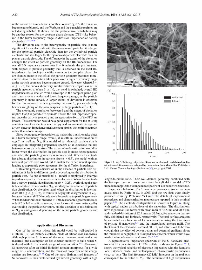
A20 Journal of The Electrochemical Society, 160 (1) A15-A24 (2013)

in the overall BD impedance smoother. When σ ≥ 0.5, the transitionbecome quite blurred, and the Warburg and the capacitive regimes arenot distinguishable. It shows that the particle size distribution maybe another reason for the constant phase element (CPE)-like behav-ior in the lower frequency range in diffusion impedance of batteryelectrodes.13,20,29,30

The deviation due to the heterogeneity in particle size is moresignificant for an electrode with the more-curved particles; it is largerfor the spherical-particle electrode than for the cylindrical-particleelectrode, and it is larger for the cylindrical-particle electrode than theplanar-particle electrode. The difference in the extent of the deviationchanges the effect of particle geometry on the BD impedance. Theoverall BD impedance curves near σ = 0 maintain the pristine trendwith respect to particle geometry that is observed in the local BDimpedance; the hockey-stick-like curves in the complex plane plotare shunted more to the left as the particle geometry becomes more-curved. Also the transition takes place over a higher frequency rangeas the particle geometry becomes more-curved. However, when 0.5 ≤σ ≤ 0.75, the curves show very similar behaviors regardless of theparticle geometry. When σ ≥ 1.0, the trend is switched; overall BDimpedance has a smaller overall envelope in the complex plane plot,and transits over a wider and lower frequency range, as the particlegeometry is more-curved. A larger extent of deviation is observedfor the more-curved particle geometry because ˜a p places relativelyheavier weighting on the local response of large particles (l > 1).

The monotonic correlation between σ and the extent of deviationimplies that it is possible to estimate σ from the BD impedance spec-tra, once the particle geometry and an appropriate form of the PDF areknown. This estimation would be a good supplement for the existingcombination of an electron microscopy and an automatic image an-alyzer, since an impedance measurement probes the entire electrode,rather than a local image.

Since heterogeneity in particle size makes the transition take placein a lower frequency range overall, it results in underestimation ofωD(L) as well as Dch , if a model of an identical particle size isemployed in interpreting impedance spectra of an electrode that hasheterogeneous particle sizes. The extent of underestimation would belarger when the distribution in particle size is more heterogeneous,and when the particle geometry is more-curved. When an electrodehas a broad distribution in particle size (σ ≥ 0.5), the model with anidentical particle size would fail to match the experimental spectra,leading to apparently poor agreement for the diffusion impedance.

Unlike the previous discussion in the absence of particle size dis-tribution, it leads to different results depending on the distribution inparticle size, if a one-dimensional zD model is employed to interpretimpedance spectra of a curved-particle electrode. When the electrodehas a narrow particle size distribution (σ ≤ 0.25), overlooking the par-ticle curvature overestimates Dch , similarly to the absence of particlesize distribution. On the other hand, when the distribution is interme-diate (0.5 ≤ σ ≤ 0.75), it results in negligible disagreement in Dch ,because the overall BD impedance is insensitive to particle geometry.When the distribution is broad (σ ≥ 1.0), reasonable agreement resultsonly if σ is left as a fit parameter; in such cases, σ is overestimated byoverlooking the particle curvature, but the direction of misestimationin Dch is ambiguous, depending on the actual particle geometry andsize distribution.

Application and Discussion

One of the systems where this model could be well-applied isa lithium (Li) ion battery electrode made of silicon (Si) nanowires.Although pristine Si is one of the most common semiconductingmaterials, the assumption of fast electron mobility is valid when Siis doped with Li for a wide range of concentration.31,32 Moreover,Si nanowires after an initial lithiation remain amorphous for a widerange of Li concentration, and the transport properties of the chargecarriers are isotropic.33–35 One of the most distinguished features ofSi nanowires is their well-defined cylindrical geometry with a high

0 50 100 150 2000

25

50

75

100

125

150

175

200

l (nm)

Np

unlithiated

lithiated

(b)

5 µm 2 µm

(a)

Figure 6. (a) SEM image of pristine Si nanowire electrode and (b) radius dis-tributions of Si nanowires, adapted by permission from Macmillan PublishersLtd: Nature Nanotechnology (Reference 36), copyright 2007.

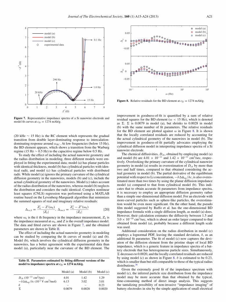
length-to-radius ratio. Their well-defined geometry combined withthe isotropic transport properties makes the cylindrical model of BDimpedance applicable to impedance spectra of a Si nanowire electrode.

Impedance behavior of a Si nanowire porous electrode has beeninvestigated by Ruffo et al., in 2009, and the raw data were kindlyprovided to us by Professor Yi Cui.8 The details of experimentalprocedures and characterization methods are reported in their originalpapers.8,36 The electrode configuration is shown in Figure 6, alongwith typical radius distributions of the nanowires. The distributionshave lognormal-like forms with mean radii of 44.5 nm and 70.5 nm,and standard deviations of 22.5 nm and 32.0 nm, for nanowires that arefully delithiated and lithiated, respectively. The total surface area canbe estimated as a function of Li concentration, using the total massof pristine Si nanowires8,36 and the interpolated average radii. Thethickness of the electrode is around 30 μm, and it turns out to be thinenough that the effect of concentration and potential gradients alongthe thickness is negligible in its impedance spectra, which would havemade the impedance curve skewed.15,16,20,37

A representative impedance spectrum of the Si nanowire elec-trode at Li concentration of 1274 mAh/g is shown in Figure 7. Itshows the typical behavior of electrode impedance with the Randle’slocal interface model and well-separated characteristic frequencies(ωRC � ωD). The high frequency (20 kHz) intercept on the real axiscorresponds to the value of Rext . The semicircle at high frequencies

Journal of The Electrochemical Society, 160 (1) A15-A24 (2013) A21

0 1 2 3 4 5 6 7 80

1

2

3

4

5

6

7

8

model (a)

model (b)

model (c)

experimental data

0.1 Hz

1.0 Hz

15 Hz

290 Hz

20 kHz

Figure 7. Representative impedance spectra of a Si nanowire electrode andmodel fit curves at cLi = 1274 mAh/g.

(20 kHz ∼ 15 Hz) is the RC element which represents the gradualtransition from double layer-dominating response to intercalation-dominating response around ωRC . At low frequencies (below 15 Hz),the BD element appears, which shows a transition from the Warburgregime (15 Hz ∼ 0.5 Hz) to the capacitive regime below 0.5 Hz.

To study the effect of including the actual nanowire geometry andthe radius distribution in modeling, three different models were em-ployed in fitting the experimental data; model (a) has planar particleswith identical thickness, model (b) has cylindrical particles with iden-tical radii, and model (c) has cylindrical particles with distributedradii. While model (a) ignores the primary curvature of the cylindricaldiffusion geometry in the nanowires, models (b) and (c), include theactual cylindrical geometry of the nanowires. Model (c) takes accountof the radius distribution of the nanowires, whereas model (b) neglectsthe distribution and considers the radii identical. Complex nonlinearleast squares (CNLS) regression was performed using a MATLABroutine based on the Levenberg-Marquardt algorithm that minimizesthe summed squares of real and imaginary relative residuals:

�re,k = Z ′k − Z ′(ωk)

|Zk | , �im,k = Z ′′k − Z ′′(ωk)

|Zk | [20]

where ωk is the k th frequency in the impedance measurement, Zk isthe impedance measured at ωk , and Z is the overall impedance model.The data and fitted curves are shown in Figure 7, and the obtainedparameters are shown in Table II.

The effect of including the actual nanowire geometry in modelingcan be studied by comparing the fit curves of model (a) and (b).Model (b), which involves the cylindrical diffusion geometry in thenanowires, has a better agreement with the experimental data thanmodel (a), particularly near the curvature of the BD element. The

Table II. Parameters estimated by fitting different versions of themodel to impedance spectra at cLi = 1274 mAh/g.

Model (a) Model (b) Model (c)

Dch (10−11 cm2/sec) 4.01 1.42 1.29−∂�φeq/∂c (10 2 V cm3/mol) 6.13 3.02 3.01σ – – 0.23� 0.0079 0.0028 0.0020

−0.05

0

0.05

10−1 1 101 102

−0.05

0

0.05

(Hz)

imre

model (a)model (b)model (c)

Figure 8. Relative residuals for the BD element at cLi = 1274 mAh/g.

improvement in goodness-of-fit is quantified by a sum of relativeresidual squares for the BD element (ω < 15 Hz), which is denotedas �. � is 0.0079 in model (a), but shrinks to 0.0028 in model(b) with the same number of fit parameters. The relative residualsfor the BD element are plotted against ω in Figure 8. It is shownthat the locally correlated residuals are reduced by accounting forthe actual cylindrical geometry of the nanowires in model (b). Theimprovement in goodness-of-fit partially advocates employing thecylindrical diffusion model in interpreting impedance spectra of a Sinanowire electrode.

The chemical diffusivities, Dch , obtained by employing model (a)and model (b) are 4.01 × 10−11 and 1.42 × 10−11 cm2/sec, respec-tively. Overlooking the primary curvature of the cylindrical nanowiregeometry in model (a) results in overestimation of Dch by more thantwo and half times, compared to that obtained considering the ac-tual geometry in model (b). The partial derivative of the equilibriumpotential with respect to Li concentration, −∂�φeq/∂c, is also overes-timated more than two times by using the planar diffusion impedancemodel (a) compared to that from cylindrical model (b). This indi-cates that to obtain accurate fit parameters from impedance spectra,it is necessary to employ an appropriate diffusion geometry ratherthan a simple one-dimensional diffusion model. For an electrode withmore-curved particles such as sphere-like particles, the overestima-tion would be even more significant. On the other hand, the pseudofilm model suggested by Ruffo et al. has the one-dimensional BDimpedance formula with a single diffusion length, as model (a) does.However, their calculation estimates the diffusivity between 1.5 and3.0 × 10−10 cm2/sec, which is about an order larger compared to thatobtained from model (a), probably because a different length scalewas used.

Additional consideration on the radius distribution in model (c)employs a lognormal PDF, leaving the standard deviation, σ, as anadditional fit parameter. The fit of model (c) now captures the devi-ation of the diffusion element from the pristine shape of local BDimpedance, which is a generic feature in impedance spectra of a bat-tery electrode that has heterogeneous particle sizes. Simultaneously,� decreases to 0.0020, and the locally correlated residuals are reducedby using model (c) as shown in Figure 8. σ is estimated to be 0.23,which is smaller than but still comparable to those of the typical radiusdistributions.36

Given the extremely good fit of the impedance spectrum withmodel (c), the inferred particle size distribution from the impedancemodel may be more accurate than that obtained by the typical,time-consuming method of direct image analysis. This suggeststhe tantalizing possibility of non-invasive “impedance imaging” ofbattery electrodes in situ by the simple application of small electrical

A22 Journal of The Electrochemical Society, 160 (1) A15-A24 (2013)

Table III. The chemical diffusivities of Li ion in amorphous Si nanowire at different Li concentrations during the second cycle.

cLi (mAh/g) Dch (10−11 cm2/sec) −∂�φeq/∂c (10 2 V cm3/mol) Cdl (10−7 F/cm2) ρct (10 2 � cm2) Rext (�)

954 1.45 2.95 7.79 6.49 1.491274 1.29 3.01 6.22 7.26 1.482385 1.18 1.78 4.67 9.81 1.472705 2.01 6.63 3.41 11.9 1.53

signals, using the diffusion impedance model to solve an inverseproblem for the particle size distribution. Such changes in particlethickness could be used, for example, to detect the state of charge(due to volume change upon lithiation) or gradual degradationover many cycles, e.g. due to the formation of solid electrolyteinterphase. While we are showing here probably one of the simplestexamples of having impedance imaging for an electrode with simpleand well-characterized microstructure, to utilize the impedanceimaging in general, one should be cautious that the impedancemodel considers appropriate configurational aspects as well as otherelectrode properties that may affect impedance behavior.

Mathematically, the inversion can be performed by choosing afunctional form (such as log-normal) for the size distribution andsolving for the best-fit parameters, as we have done here. It is alsopossible to view the inverse problem as a first-kind Fredholm integralequation for the unknown size distribution function, which can besolved by Laplace or Mellin transforms, as has been done for vari-ous inverse problems in statistical mechanics.38 Such practice wouldbe limited, however, when it involves numerical techniques that maysuffer from noise and insufficient accuracy in impedance data. On theother hand, the inversion problem may not have a unique solution,when the model is not an one-to-one mapping with respect to its fit-ting parameters because two or more physical origins raise a similarimpedance feature. In such a case, it requires additional constraintsfrom other simulations (e.g. DFT or ab initio calculations) or experi-mental studies (e.g. SEM or TEM imaging), to extract meaningful fitparameters.

Using model (c) in the regression, Dch is estimated to be 1.29 ×10−11 cm2/sec, and −∂�φeq/∂c to be 3.01× 102 V cm3/mol. Compar-ing the estimator values obtained from model (b) and (c), it is foundthat overlooking the radius distribution in model (b) results in a slightoverestimation of Dch . On the other hand, the estimator of −∂�φeq/∂cchanges little by including size distribution in the impedance model,for this particular case of a Si nanowire electrode with estimated σ of0.23. In general, the extent as well as the direction of the misestimationdue to overlooking the size distribution depends on the heterogeneityin size distribution and the actual particle geometry of an electrode.

Impedance spectra of the Si nanowire electrode at various Li con-centrations are shown in Figure 9. For the intermediate concentrations,the spectra were fitted using model (c), taking into account the cylin-drical diffusion geometry as well as the radius distribution of thenanowires. The fit curves are also plotted in Figure 9, and the fit pa-rameters obtained from the regression are shown in Table III. Dch isestimated in the range of 1.18 ∼ 2.01 × 10−11 cm2/sec, dependingon the Li concentration. These values agree well with the diffusivitiesmeasured by N. Dimov et al. for a Si powder electrode, which are 1.7and 6.4 × 10−11 cm2/sec at Li concentrations of 800 and 1200 mAh/g,respectively.39 Reported values of the Li diffusivity in amorphous Siare inconsistent and spread over a wide range, varying from the orderof 10−11 to 10−13 cm2/sec at room temperature.40–42 The excellent fitof the impedance spectrum using the known particle geometry andsize distribution suggests that our value is among the most accuratein the literature.

Limitations of the diffusion model, however, can be found at bothof low and high Li concentrations. At the low Li concentrations, itis difficult to identify either RC or BD elements in the impedancespectra. The two elements seem overlapped, and the behavior at lowfrequencies is different from the typical BD impedance observed atthe intermediate Li concentrations. The model is not able to interpret

these features. A possible explanation is that the assumption regard-ing fast electron transport is not valid at low Li concentrations, as theelectron mobility becomes orders of magnitude smaller than at higherLi concentrations.31 Although it is beyond the scope in this article,an accurate interpretation of the impedance spectra at the low Li con-centrations may involve solving simultaneous transport of Li ions andelectrons from two different kinds of interfaces: radial diffusion ofions from the electrolyte and axial diffusion of electrons from the cur-rent collector.43 On the other hand, when Li concentration approachesthe full capacity, cycled Si nanowires encounter rapid phase transfor-mation from the amorphous phase to the Li15Si4 crystalline phase.34,35

When it comes to the crystalline phase at high Li concentrations, theassumption regarding isotropic transport properties is not valid anymore, and our model would need to be modified to account for theonset of crystal anisotropy, as well as possibly the dynamics of thephase transformation.

cLi= 0 mAh/g c

Li= 109 mAh/g

cLi= 954 mAh/g c

Li= 2385 mAh/g

cLi= 2705 mAh/g c

Li= 3659 mAh/g

0 10 20 30 40 500

10

20

30

40

50

0 10 20 30 40 500

10

20

30

40

50

0 2 4 6 8 100

2

4

6

8

10

0 2 4 6 8 100

2

4

6

8

10

0 2 4 6 8 100

2

4

6

8

10

0 5 10 150

5

10

15

28 Hz

3.4 Hz

8.8 Hz

1.0 Hz

250 Hz

13 Hz

0.1 Hz

252 Hz

6.3 Hz

0.1 Hz

293 Hz

0.1 Hz

14 Hz

200 Hz

8 Hz

0.1 Hz

Figure 9. Impedance spectra and fit curves at different Li concentrationsduring the second cycle.

Journal of The Electrochemical Society, 160 (1) A15-A24 (2013) A23

Conclusions

Modern battery electrodes have nanoparticles of active materialwhich have various shapes and heterogeneous sizes. In impedancespectra of such electrodes, the responses at low frequencies correspondto the bounded diffusion of ions in the particles. While properties ofthe BD impedance are expected to essentially depend on the diffusiongeometry and the diffusion length distribution in the nanoparticles,the effects of such configurational aspects have been largely over-looked. Commercial data-processing software products only containthe one-dimensional BD impedance model and the original Warburgimpedance model, which are not able to account for these effects. Inthis study, an impedance model is proposed that accounts for curveddiffusion geometries as well as the diffusion length distribution. Usingthis model, we have investigated the ways these configurational as-pects affect interpretation of diffusion impedance spectra. The modelalso opens the possibility of conversely using impedance spectroscopyto diagnose battery electrodes in terms of the configuration-relatedstatus, in situ during a test that requires many cycles.

Various versions of the model were then applied to experimentalimpedance data of a Si nanowire electrode. Comparing the regressionresults of the different versions, we are able to show that includingeach of the cylindrical diffusion geometry and the heterogeneous ra-dius distribution of the nanowires greatly improves the fit and leads torather different, and presumably more accurate, values of the electro-chemical parameters. In general, the effects of including appropriateparticle geometry and particle size distribution in modeling dependon the actual particle geometry and size distribution of an electrode.From this study, we conclude that it is important to account for theconfigurational aspects of a battery electrode to accurately interpretdiffusion impedance.

Acknowledgment

This work was partially supported by a grant from the Samsung-MIT Alliance and by a fellowship to JS from the Kwanjeong Ed-ucational Foundation. The authors thank Professor Yi Cui at Stan-ford University for providing the raw experimental data for siliconnanowire anodes, and Professor J. R. Macdonald, Dr. Y. Basoukov,and the referees for helpful comments on the manuscript.

List of Symbols

ap average surface area of a single particle [cm2]ax average sidewall area of a planar particle [cm2]˜a p dimensionless surface area of a single particle ( ˜a p = ln−1)A electroactive surface area [cm2]Atot total electroactive surface area [cm2]AW Warburg coefficient [�/s1/2]c concentration of ionic charge carrier [mol/cm3]Cdl local double layer capacitance [F/cm2]CD∞ high-frequency-limit dimensionless extra capacitance of

bounded diffusionCD0 low-frequency-limit dimensionless capacitance of bounded

diffusionDch chemical diffusivity of positive charge carrier [cm2/s]e elementary electric charge [C]H average height of a cylindrical particle [cm]j0 exchange current density [A/cm2]jdl double layer charging current density [A/cm2]jintc intercalation current density [A/cm2]jtot total current density [A/cm2]J total current [A]k Boltzmann’s constant [eV/K]l solid-state diffusion length [cm]l dimensionless solid-state diffusion length (l = l/L)L solid-state diffusion length, a random variable [cm]L average solid-state diffusion length [cm]

L dimensionless solid-state diffusion length, a random vari-able (L = L/L)

n dimension numberNtot total number of particlesPrL probability density function of a random variable, L [cm−1]PrL probability density function of a random variable, Lqdl double layer charge [C/cm2]Rext external resistance contribution [�]Rext dimensionless external resistance contribution (Rext =

Atot Rext/ρct )t time [s]T temperature [K]x spatial variable [cm]X arbitrary variableXref arbitrary variable at reference stateX Fourier coefficient of perturbation in XzD local diffusion impedance [�cm2]zD dimensionless local diffusion impedance (zD = zD/ρD)zD0 low-frequency-limit of dimensionless local diffusion

impedance [�cm2]zD∞ high-frequency-limit of dimensionless local diffusion

impedance [�cm2]zint f local interface impedance [�cm2]zint f dimensionless local interface impedance (zint f = zint f /ρct )ZW original Warburg impedance [�]Z overall impedance [�]Zk measured impedance at frequency ωk [�]Z dimensionless overall impedance (Z = Atot Z/ρct )

Greeks

α symmetric coefficientδ Dirac delta function [cm−1]�re,k real relative residual at frequency ωk

�im,k imaginary relative residual at frequency ωk

�φ potential drop across active material/electrolyte interface[V]

�φeq equilibrium potential of intercalation reaction [V]ρct local charge transfer resistance [�cm2] (ρct = kT / j0e)ρD BD impedance coefficient [�cm2]ρD/ct dimensionless BD impedance coefficient (ρD/ct = ρD/ρct )ρD0 low-frequency-limit resistance of bounded diffusionσ standard deviation [cm]σ dimensionless standard deviation (σ = σ/L)� sum of relative residual squares for diffusion impedanceω perturbation frequency [rad or Hz]ωD diffusion characteristic frequency [rad or Hz] (ωRC =

Dch/l2)ωk kth experimental frequency [rad or Hz]ωRC RC characteristic frequency [rad or Hz] (ωRC = 1/ρct Cdl )ω dimensionless perturbation frequency (ω = ω/ωD)ωRC/D characteristic frequency ratio (ωRC/D = ωRC/ωD)η surface overpotential [V]

References

1. E. Barsoukov and J. R. Macdonald, Impedance spectroscopy : theory, experiment,and applications, p. xvii, Wiley-Interscience, Hoboken, N.J. (2005).

2. W. Lai and F. Ciucci, Journal of The Electrochemical Society, 158, A115 (2011).3. E. Warburg, Annalen der Physik, 311, 125 (1901).4. B. Bernard A, Solid State Ionics, 169, 65 (2004).5. M. D. Levi and D. Aurbach, The Journal of Physical Chemistry B, 101, 4630 (1997).6. C. Ho, I. D. Raistrick, and R. A. Huggins, Journal of The Electrochemical Society,

127, 343 (1980).7. K. Dokko, Y. Fujita, M. Mohamedi, M. Umeda, I. Uchida, and J. R. Selman, Elec-

trochimica Acta, 47, 933 (2001).8. R. Ruffo, S. S. Hong, C. K. Chan, R. A. Huggins, and Y. Cui, The Journal of Physical

Chemistry C, 113, 11390 (2009).9. J. P. Schmidt, T. Chrobak, M. Ender, J. Illig, D. Klotz, and E. Ivers-Tiffee, Journal

of Power Sources, 196, 5342 (2011).

A24 Journal of The Electrochemical Society, 160 (1) A15-A24 (2013)

10. Y.-R. Zhu, Y. Xie, R.-S. Zhu, J. Shu, L.-J. Jiang, H.-B. Qiao, and T.-F. Yi, Ionics, 17,437 (2011).

11. M. D. Levi and D. Aurbach, Electrochimica Acta, 45, 167 (1999).12. T. Jacobsen and K. West, Electrochimica Acta, 40, 255 (1995).13. J. Bisquert, G. Garcia-Belmonte, F. Fabregat-Santiago, and P. R. Bueno, Journal of

Electroanalytical Chemistry, 475, 152 (1999).14. Q. Guo, V. R. Subramanian, J. W. Weidner, and R. E. White, Journal of The Electro-

chemical Society, 149, A307 (2002).15. J. H. K. Evgenij Barsoukov, Jong Hun Kim, Chul Oh Yoon, and Hosull Lee, Solid

State Ionics, 116, 249 (1999).16. J. P. Meyers, M. Doyle, R. M. Darling, and J. Newman, Journal of The Electrochem-

ical Society, 147, 2930 (2000).17. M. D. Levi and D. Aurbach, The Journal of Physical Chemistry B, 101, 4641

(1997).18. M. D. Levi, Z. Lu, and D. Aurbach, Solid State Ionics, 143, 309 (2001).19. T. Kulova, Y. Pleskov, A. Skundin, E. Terukov, and O. Kon’kov, Russian Journal of

Electrochemistry, 42, 708 (2006).20. M. D. Levi and D. Aurbach, The Journal of Physical Chemistry B, 108, 11693

(2004).21. M. A. Vorotyntsev, A. A. Rubashkin, and J. P. Badiali, Electrochimica Acta, 41, 2313

(1996).22. D. R. Franceschetti, J. R. Macdonald, and R. P. Buck, Journal of The Electrochemical

Society, 138, 1368 (1991).23. W. Lai and S. M. Haile, Journal of the American Ceramic Society, 88, 2979

(2005).24. W. Preis and W. Sitte, Journal of the Chemical Society, Faraday Transactions, 92,

1197 (1996).25. M. Abramowitz and I. Stegun, Handbook of Mathematical Functions: with Formulas,

Graphs, and Mathematical Tables, p. 358, Dover (1964).26. J. E. B. Randles, Discussions of the Faraday Society, 1, 11 (1947).27. D. C. Grahame, Journal of The Electrochemical Society, 99, 370C (1952).

28. M. Doyle, J. P. Meyers, and J. Newman, Journal of The Electrochemical Society, 147,99 (2000).

29. J. Bisquert, G. Garcia-Belmonte, P. Bueno, E. Longo, and L. O. S. Bulhoes, Journalof Electroanalytical Chemistry, 452, 229 (1998).

30. M. D. Levi, C. Wang, and D. Aurbach, Journal of Electroanalytical Chemistry, 561,1 (2004).

31. E. Pollak, G. Salitra, V. Baranchugov, and D. Aurbach, The Journal of PhysicalChemistry C, 111, 11437 (2007).

32. W. Wan, Q. Zhang, Y. Cui, and E. Wang, Journal of Physics: Condensed Matter, 22,415501 (2010).

33. H. Kim, C.-Y. Chou, J. G. Ekerdt, and G. S. Hwang, The Journal of Physical Chem-istry C, 115, 2514 (2011).

34. T. D. Hatchard and J. R. Dahn, Journal of The Electrochemical Society, 151, A838(2004).

35. J. Li and J. R. Dahn, Journal of The Electrochemical Society, 154, A156 (2007).36. C. K. Chan, H. Peng, G. Liu, K. McIlwrath, X. F. Zhang, R. A. Huggins, and Y. Cui,

Nat Nano, 3, 31 (2008).37. S. Devan, V. R. Subramanian, and R. E. White, Journal of The Electrochemical

Society, 151, A905 (2004).38. M. Z. Bazant and B. L. Trout, Physica A: Statistical Mechanics and its Applications,

300, 139 (2001).39. N. Dimov, K. Fukuda, T. Umeno, S. Kugino, and M. Yoshio, Journal of Power

Sources, 114, 88 (2003).40. T. Kulova, A. Skundin, Y. Pleskov, E. Terukov, and O. Kon’kov, Russian Journal of

Electrochemistry, 42, 363 (2006).41. J. Xie, N. Imanishi, T. Zhang, A. Hirano, Y. Takeda, and O. Yamamoto, Materials

Chemistry and Physics, 120, 421 (2010).42. K. Yoshimura, J. Suzuki, K. Sekine, and T. Takamura, Journal of Power Sources,

146, 445 (2005).43. J. R. Macdonald and D. R. Franceschetti, Journal of Electroanalytical Chemistry and

Interfacial Electrochemistry, 99, 283 (1979).