EFFECTS OF MONETARY POLICY IN ROMANIA - A …ceswp.uaic.ro/articles/CESWP2012_IV3a_POP.pdfCEESS kWWoorrkiinngg PPaappeerrss 605 EFFECTS OF MONETARY POLICY IN ROMANIA - A VAR APPROACH

CCEESS WWoorrkkiinngg PPaappeerrss

605

EFFECTS OF MONETARY POLICY IN ROMANIA - A VAR APPROACH

Iulian Popescu

Alexandru Ioan Cuza University of Iaşi, Rom\nia [email protected]

Abstract: Understanding how monetary policy decisions affect inflation and other economic variables

is particularly important. In this paper we consider the implications of monetary policy under the inflation targeting regime in Romania, based on an autoregressive vector method including recursive VAR and structural VAR (SVAR). Therefore, we focus on assessing the extent and persistence of monetary policy effects on gross domestic product (GDP), price level, extended monetary aggregate (M3) and exchange rate. The main results of VAR analysis reflect a negative response of consumer price index (CPI), GDP and M3 and positive nominal exchange rate behaviour to a monetary policy shock, and also a limited impact of a short-term interest rate shock in explaining the consumer prices, production and exchange rate fluctuations.

Keywords: monetary policy, transmission mechanism, vector auto regressions JEL Classification: E31, E52, E58, C32

INTRODUCTION

The monetary policy transmission mechanism describes how traders respond to the decisions

of monetary authorities in the context of future, mutual interactions between them. Such a process

can be characterized as a set of monetary policy propagation channels through which the central

bank influences the aggregate demand and the prices in the economy. Thus, we underline the

presence of traditional channels of monetary policy transmission: the interest rate channel, the

exchange rate channel, the credit (banking and balance sheet), the expectations channel, particularly

important under inflation targeting regime and a series of non-standard channels such as the cost of

risk taking risk.

Linked to the above, the present paper aims to empirical analyse the effects of monetary

policy shocks on real economic aggregates and prices. Our approach is structured as follows. The

first part offers a review of the literature focused on Central and Eastern Europe research, both at

the level of individual states and for different groups within the region compared to other advanced

economies; the second part explains the VAR model and data used. The third part is centred on

identifying shocks with a distinction between recursive vector autoregressive (the Choleski

identification) and structural autoregressive vector that implies zero restrictions freely distributed

allowing for greater flexibility and a more accurate description of the considered variables

interdependence. The fourth part focuses on model robustness, on its ability to provide a good


606

image of the interactions dynamics between variables. The results on the effects of monetary policy

shocks are shown in the fifth part that also presents the shock response functions (impulse

response), decomposition of the variance (dispersion) and Granger causality. The sixth part contains

conclusions and future directions of analysis.

1. RELATED VAR LITERATURE

Autoregressive vector models (VAR) introduced by Sims (1980) are considered to prevail in

the econometric modelling of monetary policy transmission mechanism. Fry and Pagan (2005)

argued that this class of models offers the ideal combination between the data-based approach and

the coherent approach based on economic theory. With regard to monetary policy analysis, the

VAR methodology was further developed in the works of Gerlach and Smets (1995), Leeper, Sims

and Zha (1998), Christiano, Eichenbaum, and Evans (1999). The latter study provides a detailed

analysis of the literature on the subject in the U.S. Similarly, several researches have been

undertaken in Europe to study the various aspects of the monetary policy transmission mechanism

within the euro area (Angeloni, Kashyap, and Mojon, 2003). These studies focused both on the

whole euro area (Peersman and Smets, 2001), and on individual member countries (Mojon and

Peersman, 2001).

The analysis of the monetary policy transmission mechanism with VAR models spread to the

emerging markets of Central and Eastern Europe. Again, we identify individual-level studies and

comparative analyses for different groups of countries in the region.

Thus, Hurník and Arnoštová (2005) analysed the transmission mechanism of monetary policy

in the Czech Republic for the period 1994-2004 using a VAR methodology. Their results show that

an unexpected contractionary monetary policy shock leads to a lower production; prices increase in

the first two quarters after the shock (price puzzle), exchange rate drops (appreciation) for 4-5

quarters and after it raises (delayed overshooting). The transmission mechanism of monetary policy

in the Czech Republic is also studied by Morgese and Horvath (2008). The two authors take into

account the period 1998-2006 (only the inflation targeting regime time) and using VAR, SVAR and

FAVAR they obtain the following results: an unexpected contractionary monetary policy shock

causes a decrease in production and in the price level with a maximum amplitude after about a year;

and a persistent appreciation of the exchange rate followed by a further depreciation.

In Poland, Lyziak, Przystupa and Wróbel (2008) conducted an SVAR analysis of monetary

policy transmission mechanism for the period 1997Q1 - 2006Q1, a period characterized by an


607

inflation targeting regime. The empirical results obtained showed a maximum response of price

level to a positive short-term interest rate shock after 16 to 20 months ex post the event, while the

output response differs depending on the identification method used.

Demchuk et al. (2012) assessed the key characteristics of the monetary policy transmission

mechanism in Poland, using VAR and SVAR during 1998-2011 (both monthly and quarterly data)

and highlighted the following conclusions: an increase in short term interest rate by 1 % strongly

reflects on output, price level and exchange rate (consumer price index decreases by about 0.3%

after 6 quarters, the production by the same percentage after four quarters, an appreciation of the

national currency that lasts 14 to 16 quarters).

In Romania, an analysis of monetary policy transmission mechanism was conducted by

Antohi, Udrea and Braun (2003). For studying the first segment, namely the transmission of policy

decisions on financial variables, the three authors used a vector error correction model (VEC). Their

conclusion emphasized that the central bank directly influences deposit interest rate through

sterilization operations interest rate, but the banks’ lending rate does not seem to be directly

sensitive to NBR policy rate, but to deposit interest rate.

More recently, the VAR and SVAR approach of monetary policy transmission mechanism in

Romania was applied by Andries (2008). Considering the period 2000:1 - 2007:6 and Cholesky

identification method the author’s main result highlighted that a sudden increase in the effective

short-term interest rate causes a decrease in consumer prices that reflects the greatest amplitude

after 6 months and an appreciation of the national currency with a maximum recorded in the same

period after the shock.

There are also works that analyse and compare the effects of monetary policy through vector

autoregressive model in different groups of Central and Eastern European countries against other

advanced economies (Creel and Levasseur, 2005; Héricourt, 2005 ; Elbourne and de Haan, 2006,

Darvas, 2005). These studies underlined some specific features of the monetary policy transmission

mechanism in the new EU members from Central and Eastern Europe compared to the old Member

States. Such particularities include a number of elements such as: 1) financial systems relatively

less developed than the old EU member states, which could lead to a weaker impact of monetary

policy on the economy, 2) additional difficulties in anchoring inflation expectations, which may

generate prices behaviours with highest lags, 3) an increased inflation rate with considerable impact

on the monetary policy transmission mechanism because under a higher inflation environment the

agents adjust their prices more often having as a result a lower prices rigidity in these countries.


608

At the same time, these researches stresses a common view in the literature, namely the

prevalence of exchange rate channel against the other two traditional channels of monetary policy

transmission mechanism (interest rate channel and the credit) in the Central and Eastern European

countries. In addition, Creel and Levasseur (2005) highlighted the weak impact of monetary policy

in the region on production and prices, a conclusion opposite to that supported by Elbourne and de

Haan (2006).

Anzuini and Levy (2007) provided empirical evidence on the effects of monetary policy

shocks in the Czech Republic, Hungary and Poland. The VAR system estimates considered by the

two authors have suggested that despite a weaker development of national financial systems, the

responses of macroeconomic variables to a monetary policy shock are similar between the three

countries, and not significantly different from those of the advanced European economies. While

from a qualitative perspective the responses of EU new member states proved to be similar to those

observed in the old EU member states, quantitatively they were on average, weaker.

More recently, Jarociński (2010) performed a systematic comparison of macroeconomic

variables responses to monetary shocks in Western Europe and new EU member states. New

Member States (Czech Republic, Hungary, Poland and Slovenia) behaviours proved to be

qualitatively similar to those in developed countries sample (Finland, France, Italy, Portugal and

Spain), but with interesting differences: while production responses were found to be generally

similar, price reactions uncertainty included the possibility of stronger effects compared to the case

of considered Euro zone members. This result suggest that when analysing differences between the

Central and Eastern European countries and Western Europe states, the study should be much more

in depth, beyond the rule assuming that the monetary policy is less effective in countries with less

developed financial systems.

Presently there is a new wave of interest to identifying and analysing the implications of the

recent financial crisis and on the monetary policy transmission mechanism based on VAR method

(e.g. Boivin et al., 2010, Cecioni and Neri, 2010). Central and Eastern Europe countries researches

are still in their infancy. In this regard we note the study of Lyziak et al. (2011), which highlighted

the impact of recent global turmoil on the effectiveness of monetary policy transmission mechanism

in Poland through a VAR and a small structural model, with the mention that it depends on

monetary policy and the structural characteristics of the economy. The financial crisis, which

affected both components led to a change in monetary policy rule and a significant lower efficiency

of monetary policy.


609

In the same line, Demchuk et al. (2012) pointed out that during the recent international stress,

the monetary policy transmission mechanism in a small open economy such as Poland suffered

extensive disturbance, with the interest rate channel being the most affected

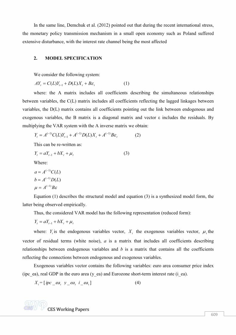
2. MODEL SPECIFICATION

We consider the following system:

tttt BXLDYLCAY )()( 1 (1)

where: the A matrix includes all coefficients describing the simultaneous relationships

between variables, the C(L) matrix includes all coefficients reflecting the lagged linkages between

variables, the D(L) matrix contains all coefficients pointing out the link between endogenous and

exogenous variables, the B matrix is a diagonal matrix and vector ε includes the residuals. By

multiplying the VAR system with the A inverse matrix we obtain:

tttt BAXLDAYLCAY )1()1(1

)1( )()(

(2)

This can be re-written as:

tttt bXaYY 1 (3)

Where:

BALDAbLCAa

)1(

)1(

)1(

)()(

Equation (1) describes the structural model and equation (3) is a synthesized model form, the

latter being observed empirically.

Thus, the considered VAR model has the following representation (reduced form):

tttt bXaYY 1

where: tY is the endogenous variables vector, tX the exogenous variables vector, t the

vector of residual terms (white noise), a is a matrix that includes all coefficients describing

relationships between endogenous variables and b is a matrix that contains all the coefficients

reflecting the connections between endogenous and exogenous variables.

Exogenous variables vector contains the following variables: euro area consumer price index

(ipc_ea), real GDP in the euro area (y_ea) and Eurozone short-term interest rate (i_ea).

tX = [ teaipc _ teay _ teai _ ] (4)


610

These variables are used to control the evolution of demand and inflation in the euro area.

Their inclusion helps solve the so-called price puzzle (e.g. the empirical results currently identified

in the VAR literature showing that the interest rate rise results in an increase of price levels).

Treating these variables as exogenous means, implicitly, that there is no impact from the

endogenous to the exogenous variables. At the same time it allows for the contemporary impact of

exogenous on endogenous variables.

Endogenous variables vector contains the following: Romanian real gross domestic product

(y_ro), the national consumer price index (ipc_ro), M3 monetary aggregate (m3_ro), domestic

short-term interest rate (i_ro) and nominal exchange rate EUR / RON (s_ro).

tY = [ troy _ troipc _ trom _3 troi _ tros _ ] (5)

Data

The data sample is restricted, including data from mid-2005, at which point the NBR adopted

inflation targeting strategy. Before this moment, during 1990-1997 the central bank applied a

monetary targeting strategy and between 1997 and 2005 a combined strategy targeting both

monetary aggregates and the exchange rate (eclectic strategy). Thus, the sample covers the period

between 2005: Q3 and 2012: Q1 with a quarterly frequency. As a result, we have 27 observations

provided by Eurostat (www.eurostat.ec.europa.eu).

The analysed variables include:

the national real gross domestic product and the euro area ( troy _ , teay _ );

fixed-base index of domestic consumer prices and the euro area indicator( troy _ , teay _ );

M3 monetary aggregate in Romania( trom _3 );

the national and Euro zone short-term interest rates with ROBOR as proxy, and respectively

3-month EURIBOR ( troi _ teai _ );

EUR / RON nominal exchange rate ( tros _ ).

All series except the interest rates and exchange rates have been adjusted to eliminate

seasonal factors based on the X12 procedure used by the U.S. Census Bureau. Also all series except

interest rates were put under logarithms.


611

The VAR variables should not be stationary. Sims (1980), inter alia, argued against

differentiation, even if the series contain a unit root, causing informational losses. What matters for

VAR results robustness is the system general stationarity (Lütkepohl, 2006).

If the considered endogenous variables are stationary, meaning integrated of order zero, I (0),

the VAR estimation is supported by level-specified variables. If the variables are nonstationary but

cointegrated, the estimation is allowed with level-specified variables or autocorrection model

(VEC). Finally, if the variables are nonstationary and not cointegrated it is necessary to specify

them as differences.

We test the stationarity with the help of Augmented Dickey - Fuller test and Phillips – Perron

test; their results indicate that variables are not stationary: y_ro_sa: I (2), y_ea_sa: I (2), ipc_ro_sa: I

(1), ipc_ea_sa: I (2), i_ro: I (1), m3_ro: I (0), i_ea: I (2), s_ro: I (1).

Cointegration testing based on the methodology developed by Johansen indicate that there are

three cointegration equations at a significance level of 0.05 (outcome based on both Trace and

Maximum Eigenvalue Tests). This result, in conjunction with the stationarity tests conclusions

underlines the possibility of model estimation with level-specified variables.

The number of lags considered must capture the system dynamics without consuming too

many degrees of freedom. If the lag number is too small, the model will not be specified correctly

and if the number is too high, too many degrees of freedom would be lost (Codirlaşu, 2007).

Choosing the number of lags was based on results synthesis of several methods: the sequential

testing of lags significance, minimizing the final prediction error and information content evaluation

criteria (Akaike, Schwartz and Hannan-Quinn). Most criteria indicate the existence of 1 lag. We

check the result by excluding non-significant lags based on lag exclusion tests. Lag Exclusion Wald

test confirmed the retaining of 1 lag.

3. SHOCKS IDENTIFICATION

Shocks identification is based on imposing zero-restrictions for A and B matrices coefficients

in BA )1( relation. The minimum number of zero restrictions to be imposed to identify

structural innovations is n (n-1) / 2, where n is the number of endogenous variables (in this case n =

5). So, if we impose a number of 10 zero-restrictions, the VAR system is precisely identified and if

the number of zero restrictions is higher than 10, the system will be over-identified. The

determination of the appropriate number of zero restrictions (innovation decomposition or


612

orthogonalization), which is actually equivalent to setting assumptions about the endogenous

variables can be done in several ways.

One of the methods is the recursive Choleski identification. In this case, the A matrix has a

triangular structure, the all elements above the main diagonal equal to zero. Under Choleski

approach, the two matrices, A and B, have the following representation:

101001000100001

54535251

434241

3231

21

aaaaaaa

aaa

A

55

44

33

22

11

00000000000000000000

bb

bb

b

B

The ordering of the variables in the context of equation (5) requires implicit assumptions

about: (i) what do the monetary authority considers when making monetary decisions, and (ii)

which are the variables that simultaneously respond or not respond to monetary policy decisions.

This ordering also implies that when deciding, the central bank takes into account the current level

of production, prices and monetary developments. At the same time, monetary policy actions have

no impact on production and prices contemporary. Because the exchange rate is ordered after the

interest rate, the latter should have an immediate impact on the exchange rate. On the other hand,

the interest rate does not respond in the same period to changes in nominal exchange rate.

The considered recursive VAR model (the Choleski identification) requires a rigid structure

of causal relationships between variables and as a result, its ability to correctly describe

dependencies between variables is put under question. To eliminate these drawbacks, namely to

allow greater flexibility of connections between variables, it is necessary to use a structural VAR

identification with Sims (1986) and Bernake (1986) identification method. Under this

orthogonalization approach the zero restrictions can be freely distributed. In the case of structural

VAR, the two matrices, A and B, are represented as follows:

1100

01000100001

54535251

4541

343231

21

aaaaaa

aaaa

A

55

44

33

22

11

00000000000000000000

bb

bb

b

B

The number of zero restrictions imposed in this case is also 10; therefore the system is exactly

identified. The first two equations represent the slow reaction of the real sector (GDP and prices) to

monetary sector shocks (M2, interest rates and exchange rates). There is no contemporary impact of


613

monetary policy shocks, M2 and exchange rate on production and prices. M2 is influenced by GDP

contemporary innovations, price level and short-term interest rate. The central bank sets the interest

rate taking into account the contemporary innovations of production ( 41a can be interpreted as a

pressure indicator of excessive demand) and exchange rate ( 45a can be interpreted as the exchange

rate fluctuations that influence inflation expectations), but it does not respond simultaneously to

monetary aggregate shocks (under a monetary targeting regime) and to price level (price

information is available only with a certain lag). Finally, the exchange rate as price of an asset

immediately reacts to all the innovations of the other variables.

4. ANALYSIS ROBUSTNESS

The VAR is confirmed if it is stable and the residuals are "white noise".

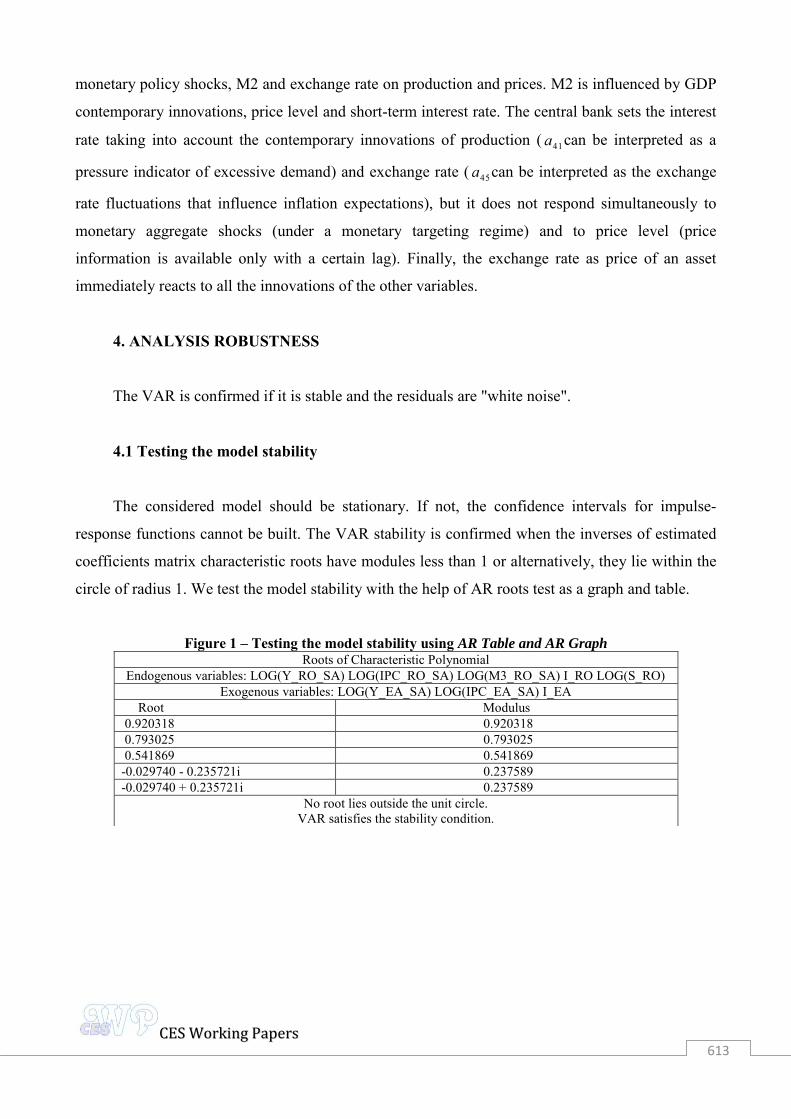
4.1 Testing the model stability

The considered model should be stationary. If not, the confidence intervals for impulse-

response functions cannot be built. The VAR stability is confirmed when the inverses of estimated

coefficients matrix characteristic roots have modules less than 1 or alternatively, they lie within the

circle of radius 1. We test the model stability with the help of AR roots test as a graph and table.

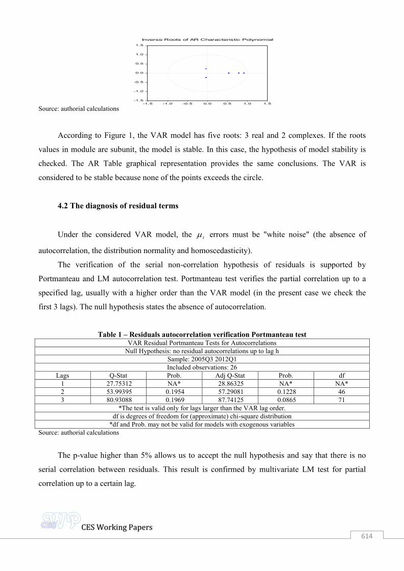
Figure 1 – Testing the model stability using AR Table and AR Graph

Roots of Characteristic Polynomial Endogenous variables: LOG(Y_RO_SA) LOG(IPC_RO_SA) LOG(M3_RO_SA) I_RO LOG(S_RO)

Exogenous variables: LOG(Y_EA_SA) LOG(IPC_EA_SA) I_EA Root Modulus 0.920318 0.920318 0.793025 0.793025 0.541869 0.541869 -0.029740 - 0.235721i 0.237589 -0.029740 + 0.235721i 0.237589

No root lies outside the unit circle. VAR satisfies the stability condition.


614

Source: authorial calculations

According to Figure 1, the VAR model has five roots: 3 real and 2 complexes. If the roots

values in module are subunit, the model is stable. In this case, the hypothesis of model stability is

checked. The AR Table graphical representation provides the same conclusions. The VAR is

considered to be stable because none of the points exceeds the circle.

4.2 The diagnosis of residual terms

Under the considered VAR model, the t errors must be "white noise" (the absence of

autocorrelation, the distribution normality and homoscedasticity).

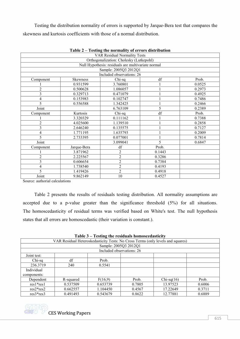
The verification of the serial non-correlation hypothesis of residuals is supported by

Portmanteau and LM autocorrelation test. Portmanteau test verifies the partial correlation up to a

specified lag, usually with a higher order than the VAR model (in the present case we check the

first 3 lags). The null hypothesis states the absence of autocorrelation.

Table 1 – Residuals autocorrelation verification Portmanteau test VAR Residual Portmanteau Tests for Autocorrelations

Null Hypothesis: no residual autocorrelations up to lag h Sample: 2005Q3 2012Q1 Included observations: 26

Lags Q-Stat Prob. Adj Q-Stat Prob. df 1 27.75312 NA* 28.86325 NA* NA* 2 53.99395 0.1954 57.29081 0.1228 46 3 80.93088 0.1969 87.74125 0.0865 71

*The test is valid only for lags larger than the VAR lag order. df is degrees of freedom for (approximate) chi-square distribution

*df and Prob. may not be valid for models with exogenous variables Source: authorial calculations

The p-value higher than 5% allows us to accept the null hypothesis and say that there is no

serial correlation between residuals. This result is confirmed by multivariate LM test for partial

correlation up to a certain lag.

-1.5

-1.0

-0.5

0.0

0.5

1.0

1.5

-1.5 -1.0 -0.5 0.0 0.5 1.0 1.5

Inverse Roots of AR Characteristic Polynomial


615

Testing the distribution normality of errors is supported by Jarque-Bera test that compares the

skewness and kurtosis coefficients with those of a normal distribution.

Table 2 – Testing the normality of errors distribution VAR Residual Normality Tests

Orthogonalization: Cholesky (Lutkepohl) Null Hypothesis: residuals are multivariate normal

Sample: 2005Q3 2012Q1 Included observations: 26

Component Skewness Chi-sq df Prob. 1 0.931599 3.760801 1 0.0525 2 0.500628 1.086057 1 0.2973 3 0.329713 0.471079 1 0.4925 4 0.153983 0.102747 1 0.7486 5 0.556588 1.342425 1 0.2466

Joint 6.763109 5 0.2389 Component Kurtosis Chi-sq df Prob.

1 3.320329 0.111162 1 0.7388 2 4.025600 1.139510 1 0.2858 3 2.646240 0.135575 1 0.7127 4 1.771195 1.635793 1 0.2009 5 2.733395 0.077001 1 0.7814

Joint 3.099041 5 0.6847 Component Jarque-Bera df Prob.

1 3.871962 2 0.1443 2 2.225567 2 0.3286 3 0.606654 2 0.7384 4 1.738540 2 0.4193 5 1.419426 2 0.4918

Joint 9.862149 10 0.4527 Source: authorial calculations

Table 2 presents the results of residuals testing distribution. All normality assumptions are

accepted due to a p-value greater than the significance threshold (5%) for all situations.

The homoscedasticity of residual terms was verified based on White's test. The null hypothesis

states that all errors are homoscedastic (their variation is constant.).

Table 3 – Testing the residuals homoscedasticity VAR Residual Heteroskedasticity Tests: No Cross Terms (only levels and squares)


Joint test: Chi-sq df Prob.

236.3719 240 0.5541 Individual components:

Dependent R-squared F(16,9) Prob. Chi-sq(16) Prob. res1*res1 0.537509 0.653739 0.7805 13.97523 0.6006 res2*res2 0.662557 1.104450 0.4567 17.22649 0.3711 res3*res3 0.491493 0.543679 0.8622 12.77881 0.6889


616

res4*res4 0.368720 0.328546 0.9748 9.586711 0.8873 res5*res5 0.596612 0.831938 0.6420 15.51190 0.4875 res2*res1 0.603138 0.854871 0.6248 15.68160 0.4754 res3*res1 0.430507 0.425221 0.9350 11.19319 0.7974 res3*res2 0.471987 0.502816 0.8897 12.27167 0.7251 res4*res1 0.649271 1.041303 0.4954 16.88105 0.3933 res4*res2 0.543754 0.670388 0.7675 14.13761 0.5885 res4*res3 0.406260 0.384885 0.9540 10.56276 0.8356 res5*res1 0.639280 0.996883 0.5242 16.62129 0.4105 res5*res2 0.487442 0.534938 0.8683 12.67350 0.6965 res5*res3 0.419257 0.406086 0.9444 10.90067 0.8156 res5*res4 0.494114 0.549410 0.8582 12.84696 0.6839


The p-value of greater than 5% allows us to accept the null hypothesis and say that the

residuals do not broke the homoscedastic hypothesis.

The results of stability testing and residual terms indicate that the considered model is able to

provide a good picture of the dynamics of interactions between variables.

5. ESTIMATION RESULTS

VAR analysis provides three important results: the shock response function (impulse

response), variance decomposition (dispersion) and Granger causality.

5.1 Impulse response function

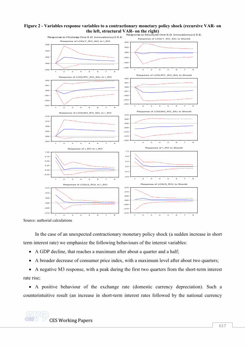
The shock response function presents the results on the effects of a monetary policy shock on

the economic variables of interest for the monetary authority. The confidence interval is 95%, the

shock is a standard deviation, and the time on the horizontal axis is expressed in quarters. Figure 2

shows the impulse-response function for considered recursive VAR and structural models.

The graphical representation points out that when using recursive VAR, a quarter of monetary

policy leads to a positive response (the same sign) of GDP, M3 and nominal exchange rate, results

that are counterintuitive.

The application of a structural VAR, for which the shock identification was achieved by the

free distribution of zero restrictions allowing for a more accurate description of the variables

interdependencies led to a negative response of GDP, CPI and M3 and positive nominal exchange

rate.


617

Figure 2 - Variables response variables to a contractionary monetary policy shock (recursive VAR- on the left, structural VAR- on the right)


In the case of an unexpected contractionary monetary policy shock (a sudden increase in short

term interest rate) we emphasize the following behaviours of the interest variables:

A GDP decline, that reaches a maximum after about a quarter and a half;

A broader decrease of consumer price index, with a maximum level after about two quarters;

A negative M3 response, with a peak during the first two quarters from the short-term interest

rate rise;

A positive behaviour of the exchange rate (domestic currency depreciation). Such a

counterintuitive result (an increase in short-term interest rates followed by the national currency

-.002

.000

.002

.004

.006

1 2 3 4 5 6 7 8

Response of LOG(Y_RO_SA) to I_RO

-.003

-.002

-.001

.000

.001

.002

1 2 3 4 5 6 7 8

Response of LOG(IPC_RO_SA) to I_RO

-.004

.000

.004

.008

.012

.016

1 2 3 4 5 6 7 8

Response of LOG(M3_RO_SA) to I_RO

-0.25

0.00

0.25

0.50

0.75

1.00

1 2 3 4 5 6 7 8

Response of I_RO to I_RO

-.010

-.005

.000

.005

.010

.015

1 2 3 4 5 6 7 8

Response of LOG(S_RO) to I_RO

Response to Cholesky One S.D. Innovations ± 2 S.E.

-.006

-.004

-.002

.000

.002

.004

1 2 3 4 5 6 7 8

Response of LOG(Y_RO_SA) to Shock4

-.004

-.003

-.002

-.001

.000

.001

.002

1 2 3 4 5 6 7 8

Response of LOG(IPC_RO_SA) to Shock4

-.020

-.015

-.010

-.005

.000

.005

.010

1 2 3 4 5 6 7 8

Response of LOG(M3_RO_SA) to Shock4

-0.8

-0.4

0.0

0.4

0.8

1.2

1 2 3 4 5 6 7 8

Response of I_RO to Shock4

-.015

-.010

-.005

.000

.005

.010

.015

1 2 3 4 5 6 7 8

Response of LOG(S_RO) to Shock4

Response to Structural One S.D. Innovations ± 2 S.E.


618

depreciation) is often found when using vector autoregressive methods, known as the "exchange

rate puzzle". This puzzle leads to higher import prices enhancing the acceleration of domestic

inflation, especially in a small open economy as Romania.

However, the results can be challenged as we note the presence of the 0 value within the

confidence interval, which translates into a lack of response to shocks (results are not statistically

significant).

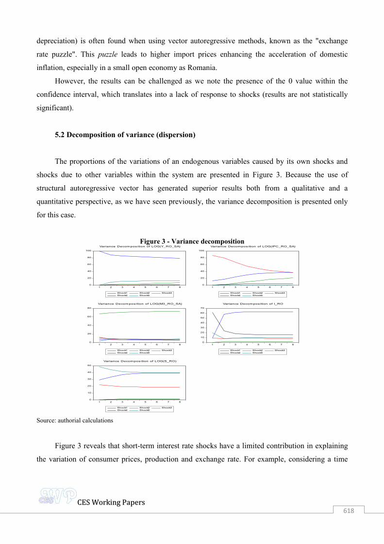
5.2 Decomposition of variance (dispersion)

The proportions of the variations of an endogenous variables caused by its own shocks and

shocks due to other variables within the system are presented in Figure 3. Because the use of

structural autoregressive vector has generated superior results both from a qualitative and a

quantitative perspective, as we have seen previously, the variance decomposition is presented only

for this case.

Figure 3 - Variance decomposition


Figure 3 reveals that short-term interest rate shocks have a limited contribution in explaining

the variation of consumer prices, production and exchange rate. For example, considering a time

0

20

40

60

80

100

1 2 3 4 5 6 7 8

Shock1 Shock2 Shock3Shock4 Shock5

Variance Decomposition of LOG(Y_RO_SA)

0

20

40

60

80

100

1 2 3 4 5 6 7 8


Variance Decomposition of LOG(IPC_RO_SA)

0

20

40

60

80

1 2 3 4 5 6 7 8


Variance Decomposition of LOG(M3_RO_SA)

0

10

20

30

40

50

60

70

1 2 3 4 5 6 7 8


Variance Decomposition of I_RO

0

10

20

30

40

50

1 2 3 4 5 6 7 8


Variance Decomposition of LOG(S_RO)


619

horizon of two quarters, the CPI variation is explained by approximately 80% of GDP shocks, 15%

by its own innovations and 2% by the monetary aggregate M3 innovations, interest rate short-term,

and nominal exchange rate. For a longer time span (8 quarters), the CPI variation is explained by

40% of GDP shocks, 40% by their innovations, 15% of innovations in M3 and less than 2% by

short-term interest rate and nominal exchange rate shocks. In the same period, the GDP variation is

explained by approximately 80% of its own innovations, 10% by the nominal exchange rate shocks,

5% by the innovations of M3 and less than 2% by the consumption price index shocks and short-

term interest rate.

5.3 Granger causality test

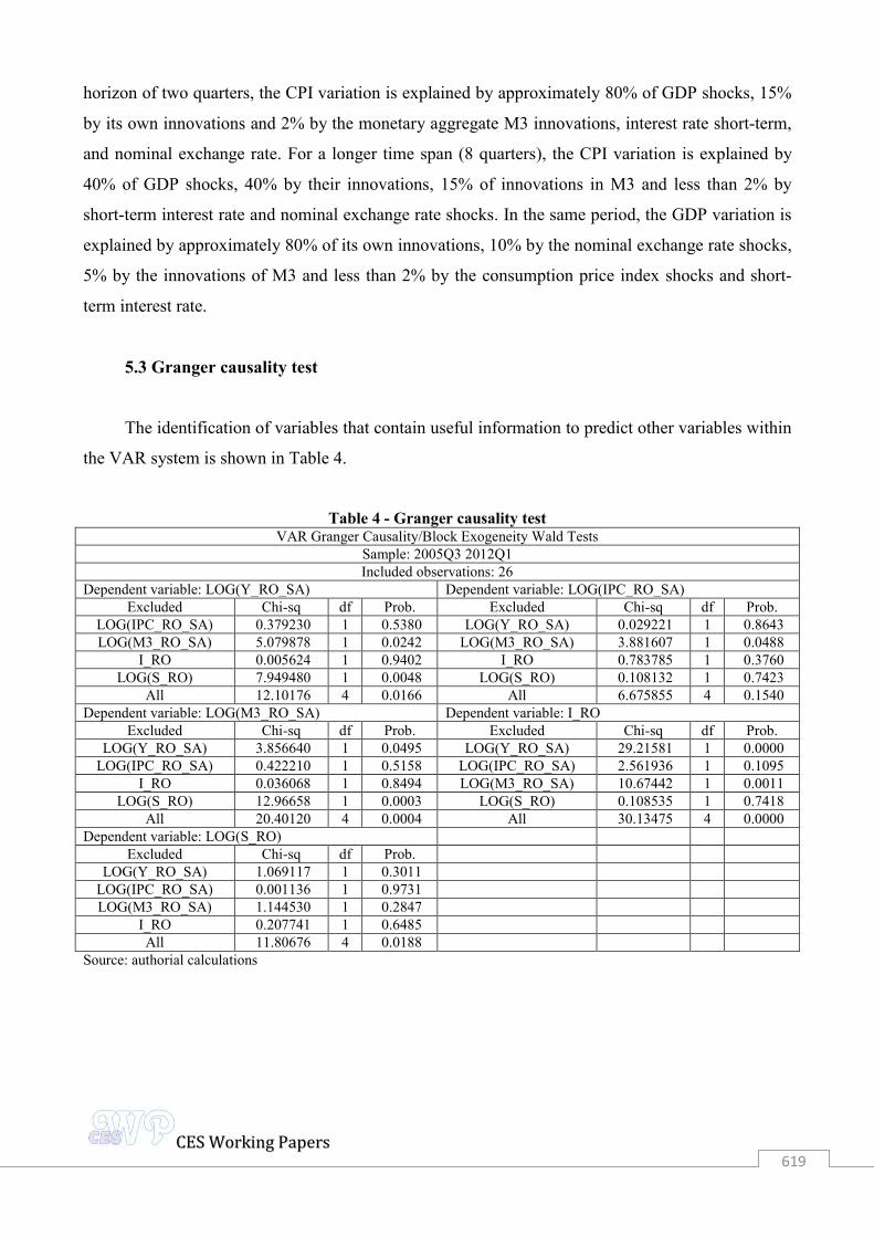
The identification of variables that contain useful information to predict other variables within

the VAR system is shown in Table 4.

Table 4 - Granger causality test VAR Granger Causality/Block Exogeneity Wald Tests


Dependent variable: LOG(Y_RO_SA) Dependent variable: LOG(IPC_RO_SA) Excluded Chi-sq df Prob. Excluded Chi-sq df Prob.

LOG(IPC_RO_SA) 0.379230 1 0.5380 LOG(Y_RO_SA) 0.029221 1 0.8643 LOG(M3_RO_SA) 5.079878 1 0.0242 LOG(M3_RO_SA) 3.881607 1 0.0488

I_RO 0.005624 1 0.9402 I_RO 0.783785 1 0.3760 LOG(S_RO) 7.949480 1 0.0048 LOG(S_RO) 0.108132 1 0.7423

All 12.10176 4 0.0166 All 6.675855 4 0.1540 Dependent variable: LOG(M3_RO_SA) Dependent variable: I_RO

Excluded Chi-sq df Prob. Excluded Chi-sq df Prob. LOG(Y_RO_SA) 3.856640 1 0.0495 LOG(Y_RO_SA) 29.21581 1 0.0000

LOG(IPC_RO_SA) 0.422210 1 0.5158 LOG(IPC_RO_SA) 2.561936 1 0.1095 I_RO 0.036068 1 0.8494 LOG(M3_RO_SA) 10.67442 1 0.0011

LOG(S_RO) 12.96658 1 0.0003 LOG(S_RO) 0.108535 1 0.7418 All 20.40120 4 0.0004 All 30.13475 4 0.0000

Dependent variable: LOG(S_RO) Excluded Chi-sq df Prob.

LOG(Y_RO_SA) 1.069117 1 0.3011 LOG(IPC_RO_SA) 0.001136 1 0.9731 LOG(M3_RO_SA) 1.144530 1 0.2847

I_RO 0.207741 1 0.6485 All 11.80676 4 0.0188



620

Granger causality tests highlight the following results:

The consumer price index variable is Granger caused by the gross domestic product variables,

short-term interest rate and nominal exchange rate, but not the monetary aggregate and it Granger

determines all other variables.

The gross domestic product is Granger caused by the consumer price index variables and

short-term interest rate, but not the nominal exchange rate and monetary aggregate M3 and it

Granger determines the nominal exchange rate and consumer price index variables.

The M3 variable is Granger caused by short-term interest rate variables and the consumer

price index, but not the nominal exchange rate variables and gross domestic product and it Granger

causes only the nominal exchange rate.

The interest rate term is Granger caused by the nominal exchange rate and consumer price

index, but not the GDP and M3 variables and it Granger determines all other variables.

The nominal exchange rate is Granger caused by all other variables and it Granger determines

the short-term interest rate and consumer price index variables.

However, it should be stressed that the Granger causality cannot be interpreted as a structural

causality, it is only consistent with (it is neither necessary nor sufficient for) true causality, the

effect must succeed in time to cause Botel (2002).

CONCLUSIONS

The three important results provided by the VAR analysis of the monetary policy transmission

mechanism were:

Shock response function (impulse response): under the considered recursive VAR

approach (the Choleski identification) a monetary policy shock causes a response of the same sign

from the GDP, M3, nominal exchange rate, results that are counterintuitive and a negative response

of price level. The free distribution of zero restrictions to identify shocks in the structural VAR

model revealed the negative behaviour of GDP, consumer price index and monetary aggregate M3

and a positive reaction of nominal exchange rate. Thus, in case of SVAR, the results of an

unexpected short-term interest rates translate into a decrease in GDP, that reaches a maximum level

after about a quarter and a half after the event; a reduction of the broad consumer price index, with a

maximum reached after about two quarters ex post the shock; a decrease of monetary aggregate M3,

with a maximum during the first two quarters after the short-term interest rate rise and an increase


621

of the exchange rate (the depreciation of the domestic currency), known as the so-called "exchange

rate puzzle".

Decomposition of variance (dispersion): short-term interest rate shocks have a reduced

role in explaining the variation of consumer prices, production and exchange rate. Regarding the

price level, for a time horizon of two quarters, the CPI variation is explained by approximately 80%

of GDP shocks, 15% of its own innovations, fewer than 2% of M3 innovations, short-term interest

rate and nominal exchange rate. For a longer time span (8 quarters), the CPI variation is explained

by approximately 40% of GDP shocks, 40% of its own innovations, 15% of innovations in M3 and

less than 2% of short-term interest rate and nominal exchange rate shocks.

Granger causality test type: short-term interest rate Granger causes CPI, GDP and M3

monetary aggregate and nominal exchange rate is Granger caused by nominal exchange rate and

consumer price index and but not by the gross domestic product and the M3 monetary aggregate.

As future directions of analysis we propose an evaluation based on the technique using an

autoregressive structural vector of the disturbance degree of monetary policy transmission

mechanism on both its segments, in the light of the recent economic and financial crisis impact and

also the determination of its efficiency under the current international financial stress.

REFERENCES

Andrieş, M., A. (2008) Monetary policy transmission mechanism in Romania - a VAR approach,

Financial and monetary policies in European Union, accessed on July 2012 at

http://www.asociatiaeconomistilor.ro/documente/Conferinta_FABBV_engleza.pdf.

Angeloni, I., Kashyapk, A., Mojon, B. (2003) Monetary Policy Transmission in the Euro Area,

European Central Bank, Working Paper No. 240, accessed on July 2012 at

http://www.ecb.europa.eu/pub/pdf/scpwps/ecbwp240.pdf.

Antohi, D., Udrea, I., Braun, H. (2003) Mecanismul de transmisie a politicii monetare în România,

Caiet de studii nr.13/ 2003, BNR, accessed on July 2012 at

http://www.bnro.ro/PublicationDocuments.aspx?icid=6786.

Anzuini, A., Levy, A. (2007) Monetary policy shocks in the new EU members: a VAR approach.

Applied Economics 39(9), pp.1147–1161, accessed on June 2012 at

http://english.mnb.hu/Root/Dokumentumtar/ENMNB/Kutatas/mnben_konf_fomenu/mnben_3

rdconference/anzuini.pdf.


622

Bernake, B. (1986) Alternative explanations of money-income correlation, Carnegie-Rochester

Conference Series on Public Policy 25, accessed on July 2012 at

http://www.nber.org/papers/w1842.

Boivin, J., Kiley, M.T., Mishkin, F.S. (2010) How has the monetary transmission mechanism

evolved over time?, NBER Working Paper No 15879, accessed on July 2012 at

http://www.nber.org/papers/w15879.

Boţel, C. (2002) Cauzele inflaţiei în România, iunie 1997-august 2001. Analiză bazată pe vectorul

autoregresiv structural, Caiet de studii nr.11/ 2002, BNR, accessed on July 2012 at

http://www.bnro.ro/PublicationDocuments.aspx?icid=6786.

Cecioni, M., Neri, S. (2010) The monetary transmission in the euro area: has it changed and why?

accessed on July 2012 at http://www.dynare.org/DynareConference2010/Cecioni_Neri

MTM_mar2010.pdf.

Creel, J., Levasseur, S. (2005) Monetary Policy Transmission Mechanisms in the CEECs: How

Important are the Differences with the Euro Area?, OFCE Working Paper, No 2, accessed on

July 2012 at http://www.ofce.sciences-po.fr/pdf/dtravail/WP2005-02.pdf.

Christiano, L., Eichenbaum, M., Evans, C. (1999) Monetary Policy Shocks: What Have We Learned

and To What End? in: TAYLOR, J., WOODFORD, M., eds., Handbook of Macroeconomics

North Holland, pp. 65–148., accessed on July 2012 at http://www.nber.org/papers/w6400.

Codirlaşu, A., Chidesciuc, N.A. (2007) Econometrie aplicată utilizând Eviews 5.1., ASE, Bucureşti,

accessed on July 2012 at http://www.dofin.ase.ro/acodirlasu/lect/econmsbank/

/econometriemsbank2007.pdf.

Darvas, Z. (2005) Monetary Transmission in the New Members of the EU: Evidence from Time-

Varying Coefficient Structural VARs, ECOMOD 2005 conference, accessed on June 2012 at

http://www.oenb.at/en/img/feei_2006_1_special_focus_4_tcm16-43659.pdf.

Demchuk, O., Łyziak, T., Przystupa, J., Sznajderska, A., Wróbel, E. (2012) Monetary policy

transmission mechanism in Poland. What do we know in 2011?, Poland National Bank,

Working Paper No. 116, accessed on July 2012 at

http://www.nbp.pl/publikacje/materialy_i_studia/116_en.pdf.

Elbourne, A., De Haan, J. (2006) Financial Structure and Monetary Policy Transmission in

Transition Countries, Journal of Comparative Economics 34, pp. 1–23, accessed on June

2012 at http://www.sciencedirect.com/science/article/pii/S0147596705000880.

http://www.bnro.ro/PublicationDocuments.aspx?icid=6786

http://www.dofin.ase.ro/acodirlasu/lect/econmsbank/econometriemsbank2007.pdf


623

Fry, R., Pagan, A. (2005) Some Issues in Using VARs for Macroeconometric Research, CAMA

Working Papers, No 19/2005, The Australian National University, accessed on July 2012 at

http://cbe.anu.edu.au/research/papers/camawpapers/Papers/2005/Fry_Pagan_182005.pdf.

Gerlach, S., Smets, F. (1995) The Monetary Transmission Mechanism: Evidence from the G-7

Countries, CEPR Discussion Paper No. 1219, accessed on May 2012 at

http://www.bis.org/publ/work26.pdf.

Héricourt, J. (2005): Monetary Policy Transmission in the CEECs: Revisited Results Using

Alternative Econometrics, University of Paris, accessed on July 2012 at ftp://mse.univ-

paris1.fr/pub/mse/cahiers2005/Bla05020.pdf.

Hurník, J., Arnoštová, K. (2005) The Monetary Transmission Mechanism in the Czech Republic:

Evidence from VAR Analysis, CNB, Working Paper Series No 4/2005, accessed on June 2012

at http://www.cnb.cz/en/research/research_publications/cnb_wp/2005/cnbwp_2005_04.html.

Jarociński, M. (2010) Reponses to Monetary Policy Shocks in the East and the West of Europe. A

Comparison, European Central Bank, Working Paper No 970, accessed on June 2012 at

http://www.ecb.europa.eu/pub/pdf/scpwps/ecbwp970.pdf.

Leeper, E., Sims, C., Zha, T. (1998) What Does Monetary Policy Do?, Brookings Papers on

Economic Activity 2, pp. 1–63, accessed on May 2012 at

http://www.benoitmojon.com/pdf/Leeper_sims_zha.pdf.

Lütkepohl, H. (2006) New Introduction to Multiple Time Series Analysis, 2nd ed., New York,

Springer, accessed on July 2012 at http://thiqaruni.org/res3/(78).pdf.

Łyziak, T., Przystupa, J., Wróbel, E. (2008) Monetary policy transmission in Poland: a study of the

importance of interest rates and credit channels, SUERF Studies, No 1, accessed on July

2012 at http://www.suerf.org/download/studies/study20081.pdf.

Łyziak, T., Przystupa, J., Stanisławska, E., Wróbel, E. (2011) Monetary policy transmission

disturbances during the financial crisis. A case of an emerging market economy, Eastern

European Economics, No. 49(5), pp. 30-51, accessed on July 2012 at

http://www.nbp.pl/badania/konferencje/2011/suerf-nbp/pdf/2011_suerfnbp_ms_e_wrobel.pdf.

Mojon, B., Peersman, G. (2001) A VAR Description of the Effects of Monetary Policy in the

Individual Countries of the Euro Area, European Central Bank, Working Paper No 92,

accessed on June 2012 at http://www.ecb.de/pub/pdf/scpwps/ecbwp092.pdf.

Morgese, M., B., Horváth, R. (2008) The Effects of Monetary Policy in the Czech Republic: An

Empirical Study, CNB, Working Paper Series No 4/2008, accessed on June 2012 at

http://www.cnb.cz/en/research/research_publications/cnb_wp/2008/cnbwp_2008_04.html.

http://www.cnb.cz/en/research/research_publications/cnb_wp/2005/cnbwp_2005_04.html

http://www.ecb.europa.eu/pub/pdf/scpwps/ecbwp970.pdf

http://www.benoitmojon.com/pdf/Leeper_sims_zha.pdf

http://thiqaruni.org/res3/(78).pdf

http://www.suerf.org/download/studies/study20081.pdf

http://www.nbp.pl/badania/konferencje/2011/suerf-nbp/pdf/2011_suerfnbp_ms_e_wrobel.pdf


624

Peersman, G., Smets, F. (2001) The Monetary Transmission Mechanism in the Euro Area: More

Evidence from VAR Analysis, European Central Bank, Working Paper No 91, accessed on

July 2012 at http://www.ecb.de/pub/pdf/scpwps/ecbwp091.pdf.

Sims, C. (1980) Macroeconomics and Reality, Econometrica 48, pp. 1–48., accessed on June 2012

at http://www.eduardoloria.name/articulos/Sims.pdf.

Sims, C. (1986) Are forecasting models usable for policy analysis?, Quarterly Review, Federal

Reserve Bank of Minneapolis, accessed on July 2012 at

http://minneapolisfed.org/research/qr/qr1011.pdf.