Embed Size (px)
Citation preview

Raquel Florez-Lopez, [email protected]
“Effects of missing data in credit risk scoring. A comparative analysis of methods to gain robustness in presence of sparce data”
Raquel Flórez-LópezDepartment of Economics and Business Administration
University of León (SPAIN)
CreditCredit ResearchResearch CentreCentreCreditCredit ScoringScoring andand CreditCredit Control XControl X
29-31 August 2007The University of Edinburgh - Management School

Raquel Florez-Lopez, [email protected]
AgendaAgenda
1. Introduction
2. Effects of missing data in credit risk scoring. A LDP perspective4.1. Managing sparce default records and missing data
4.2. The case of Low Default Portfolios (LDPs)
3. Dealing with missing values. A methodological analysis
4. Empirical research. The Australian credit approval dataset
5. Conclusions and remarks

Raquel Florez-Lopez, [email protected]
The Basel II Capital Agreement (2004) provides a ‘risk-sensitive’framework for credit risk management in banks
The Internal Ratings based (IRB) Approach uses each bank’s internal data to estimate some risk components:
Potential loss (market-based approach)PD, LGD (PD/LGD approach)
Equity exposures
MPD, LGD, EAD
MPD, LGD, EAD
Retail exposures
-PD, LGD, EAD, M
LGD, EAD, MPDCorporate, sovereign and bank exposures
Supervisory estimates
Internal estimates
Supervisory estimates
Internal estimates
IRB - ADVANCEDIRB - FOUNDATIONExposure
Internal Data are considered as the primary source of information for theestimation of the probability of default (PD) for retail exposures.
Effects of missing data in credit risk scoringEffects of missing data in credit risk scoring

Raquel Florez-Lopez, [email protected]
Rating assignements and PD estimates could consider creditscoring models based on statistical default models andhistorical databases (BCBS, 2004)
Requirements: accuracy, completeness, unbiased, appropiatenessof data, validation procedure
Use of an extensive database with enough cases
Internal records: incomplete, insufficient, missing values (Carey and Hrycay, 2001)
Low Default Portfolios (LDPs)
Characterized by sparce default records
At least 50% of the wholesale assets and a material proportion of retailportfolios could be considered as LDPs (BBA, 2004)
Difficult design of statistically significant IRB models (Benjaminet al, 2006)
Rise supervisory concern (BCBS, 2006)
Effects of missing data in credit risk scoringEffects of missing data in credit risk scoring

Raquel Florez-Lopez, [email protected]
Effects of missing data in credit risk scoringEffects of missing data in credit risk scoring
Long term Short term
Systematic
Institutionspecific
LDPs Type II
Have a low number ofcounterparties
E.g.: train operating companies
LDPs Type I
Historically have experienced a low number of defaults
Are considered to be low-riskE.g.: Banks, sovereigns, insurance
companies, highly rated firms
LDPs Type IV
May have not incurred recentlosses, but historical experience
might suggest that there is a greater likelihood of losses
E.g.: retail mortgages in somejurisdictions
LDPs Type III
Have a lack of historical data (sparce datasets)
E.g.: Being a new entrant into a marketor operating in an emerging market
FSA, 2005

Raquel Florez-Lopez, [email protected]
Effects of missing data in credit risk scoringEffects of missing data in credit risk scoring
The BCBS Directive on Low Default Portfolios (BCBS, 2005)
Alternative data sources
Alternative data-enhancing tools
Pooling data with other banks
Models for improving data input quality
More complex validation tools
Data
Based on historical experience (nor purely on human judgements)
Different categories could be combined (AAA+AA+A, etc)
Ratings
Estimates based on very prudent principles (pessimistic PD)
Confidence intervals (upper bound)
PD

Raquel Florez-Lopez, [email protected]
Missing data in LDPs (OeNB, 2004)
Handling missing values in credit risk datasets (OeNB, 2004)
Effects of missing data in credit risk scoringEffects of missing data in credit risk scoring
Missing values dramatically reduce the number and quality of observationdata.
Missing values affect to statistical estimators and confidence intervals.
Missing values affect the frequency an exogenous variables cannot be calculated in relation to the overall sample of cases
Excluding caseswith missing
values
Often impracticableSamples could be
rendered invalid
Excludingindicators
with missingvalues
If missing >20%, they can not be
statistically validhandled
Includingmissing values
as a separatecategory
Very difficult toapply in developing
scoring functionsfrom quantitative
data
Replacingmissing valueswith estimated
values
The best methoddepends on the
nature of missingvalues

Raquel Florez-Lopez, [email protected]
AgendaAgenda
1. Introduction
2. Effects of missing data on credit risk scoring. A LDP perspective4.1. Managing sparce default records and missing data
4.2. The case of Low Default Portfolios (LDPs)
3. Dealing with missing values. A methodological analysis
4. Empirical research. The Australian credit approval dataset
5. Conclusions and remarks

Raquel Florez-Lopez, [email protected]
Dealing with missing valuesDealing with missing values
Causes of missing values (Ibrahim et al, 2005; Horton and Kleinman, 2007):
Items nonresponse; missing by design; partial nonresponse; previous data aggregation; loss of data, etc.
Nature of missing values (Rubin, 1976; Little and Rubin, 2002)
Assumption Acronym R could be predicted by
Missing completely at random
Missing at random
Not missing at random (non ignorable)
MCAR
MAR
MNAR, NINR, NI
-
Xobs
Xobs and Xmis
Let D be the data matrix collected on a sample of n subjects, where f(Yi│Xi, β).For a given subject, X could be partitioned into components denoting observed variables (Xobs) and missing values (Xmis). Denote R a set of response indicators (i.e., Rj=1 if the j-th element of X is observed, 0 otherwise)
Monotony of missing values (Horton and Kleinman, 2007)
Monotone: If Xb for a subject implies that Xa is observed, for a<b
Not monotone: Otherwise

Raquel Florez-Lopez, [email protected]
Effects of missing data on credit risk scoringEffects of missing data on credit risk scoring
Listwise deletion orcomplete-case analysis
The most commonly technique used in practice for dealingwith missing data
The analysis only considers the set of completely observedsubjects
ADVANTAGES: Simplicity, comparability of univariatestatistics
LIMITATIONS: Loss of information, biased parameterestimates if data are not MCAR
VARIANT: Aplication-specific list-wise deletionIncludes all cases where the variable of interest in a specific aplication is presented.
The sample base changes from variable to variable
Bias problems if data are not MCAR.

Raquel Florez-Lopez, [email protected]
Effects of missing data on credit risk scoringEffects of missing data on credit risk scoring
Substitution approachesand ‘ad hoc’ methods
Simple imputation methods that make use of correlationamong predictors to dealing with missing data
OTHER ‘AD HOC’ METHODS: Recoding missing values, including an indicator of missingness, dropping variables with a large percentage of missing data
LIMITATIONS: Biased parameters, understandingvariability, unreliable performance, require ad hocadjustments
VARIANTS:
Imputing unconditional mean (or median/mode)
Imputing conditional mean (linear regression)
Last value carried forward: for longitudinal studies

Raquel Florez-Lopez, [email protected]
Effects of missing data on credit risk scoringEffects of missing data on credit risk scoring
Implicitly assumes than missingness is MAR
ADVANTAGES: Fast and deterministic convergence, adapted for models with known NMAR missing data (rounded and grouped data)
LIMITATIONS: Local maximum, not estimating theentire density, ignoring estimation uncertainty(biased standard errors and point estimates)
Maximum Likelihood(ML)
When some predictors have missing values, informationabout f(Y│X, β) could be inferred through estimating thedistribution of covariates f(X│γ), and the joint distributionf(X,Y│β,γ) is maximized through two steps (EM algorithm):
=
.E-step: )ˆ,ˆ,(~Σ= µobsmismis XXMLX
M-step: )~,,(ˆ,ˆ misobs XXML Σ=Σ µµ

Raquel Florez-Lopez, [email protected]
Effects of missing data on credit risk scoringEffects of missing data on credit risk scoring
Replaces each missing values by m>1 simulated values(uncertainty)
EM with sampling (EMs): based on simulations, begins with EM and adds back uncertainty to getdraws from the correct posterior distribution of Xmis
m plausible versions of the complete dataset exist; each oneis analyzed using complete-case models and results are combined:
=
.
Multiple Imputation (MI)
∑=
=m
jj mqq
1
/ˆ ∑=
⎟⎠⎞
⎜⎝⎛ +⋅+=
m
jj m
BqESm
qES1
22 11ˆ)(ˆ1)ˆ(ˆ
IP algorithm: based on MCMC, two steps considerrandom draws for (iterated): Σ̂,µ̂
)ˆ,ˆ,(~~Σµobsmismis XXPXI-step:
P-step: )~,,(ˆ,ˆ misobs XXP Σ=Σ µµ
εβ ~~~ +⋅= obsmis XX )~,~(ˆ Σ= µθ vec

Raquel Florez-Lopez, [email protected]
Effects of missing data on credit risk scoringEffects of missing data on credit risk scoring
=
.
Multiple Imputation (MI)
Other MI methods: (1) the Conditional Gaussian; (2) Chained Equations; (3) Predictive MatchingMethod
EM with importance resampling (EMis): Improvement of EMs; parameters are put onunbounded scales to obtain better results in presence of small datasets.
An acceptance-rejection algorithm is used:
))~(,~~()(θθθ
θ
VNXL
IR obs=
EM with bootstrapping (EMB): Approaches samplesof by a bootstrapping algorithm (missingtheories of inference)
Σ,µ
A key issue is the specification of the imputationmodel. If some variables are not Gaussian, MI couldlead to bias for multiple covariates.

Raquel Florez-Lopez, [email protected]
Effects of missing data on credit risk scoringEffects of missing data on credit risk scoring
Fit a model for the probability of missingness; inverse ofthese probabilities are used as weights for complete cases.
Intratable for multiple non-monotone missing variables.
Expectation-Robust (ER): Modifies the M-step of EM toinclude case weights based on Mahalanobis distance
Weighting methods
ERTBS algorithm: Departs from ER but consider bothcase weights and TBS estimator
Fully BayesianApproaches
Require specific priors on all parameters and specificdistributions for missing covariates.
Empirical results suggest that perform similarly to ML and MI
NoneML, IP, FB, WMML, IP, FB, WMNon-monotoneNoneAll but LDAllMonotoneMNARMARMCARModelModel selectionselection

Raquel Florez-Lopez, [email protected]
AgendaAgenda
1. Introduction
2. Effects of missing data in credit risk scoring. A LDP perspective4.1. Managing sparce default records and missing data
4.2. The case of Low Default Portfolios (LDPs)
3. Dealing with missing values. A methodological analysis
4. Empirical research. The Australian credit approval dataset
5. Conclusions and remarks

Raquel Florez-Lopez, [email protected]
Empirical ResearchEmpirical Research
The Australian Credit Approval Dataset
Brief description
– Credit card applications from 690 individuals (Australian bank).
– Non an extremely sparce-data retail portfolio (typically includes at least 10,000 records) (Jacobson and Roszbach, 2003; Staten and Cate, 2003; OeNB, 2004).
– 307 creditworthy (44.5%); 383 not creditworthy (55.5%).
– 14 exogenous variables: 6 continous; 8 categorical.
– Good example of mixture attributes: continous, nominal with small number of values, nominal with large number of values.
Data Data andand SampleSample
Missing values:
– 37 individuals with one or more missing values (5.36%).
– Missing values affect 6 features (40.00%): 2 continous, 4 categorical.
– Highest number of missing values per variable: 13 (1.88%).
– Previously analysed using substitution approaches (mean and mode): Quinlan (1987), Quinlan (1992), Baesens et al. (2000), Eggermont et al. (2004), Huang et al (2006).

Raquel Florez-Lopez, [email protected]
Empirical ResearchEmpirical Research
Data Data andand SampleSample
The Australian Credit Approval Dataset
First stage: ANALYSIS OF COVARIATES– Some feature selection algorithms previously applied: Cavaretta and Chellapilla (1999); Huang
et al. (2001).
– No feature selection process applied for handling missing values (King et al., 2001).
– At least p(p+3)/2 observations needed for computational efficience: 119 records (<690).
Second stage: MODELLING THE PROBLEM– Binary logistic regression to model the final class atribute Ibrahim et al. (2005); Horton and
Kleinman (2007).
– Six methods for dealing with missing data are considered: (1) listwise deletion or CC; (2)unconditional mean/median substitution or MS; (3) EM algorithm; (4) IP algorithm; (5) EMisalgorithm; (6) EMB algorithm.
– Missing data are non-monotone MAR (dichotomous continous correlations) (Hair et al, 1999).
– Variables are not jointly multivariate normal density (K-S tests).
– Comparisons are based on: β estimates, standard errors, odds ratio, p values and 95% intervals for β estimates.

Raquel Florez-Lopez, [email protected]
Empirical ResearchEmpirical Research
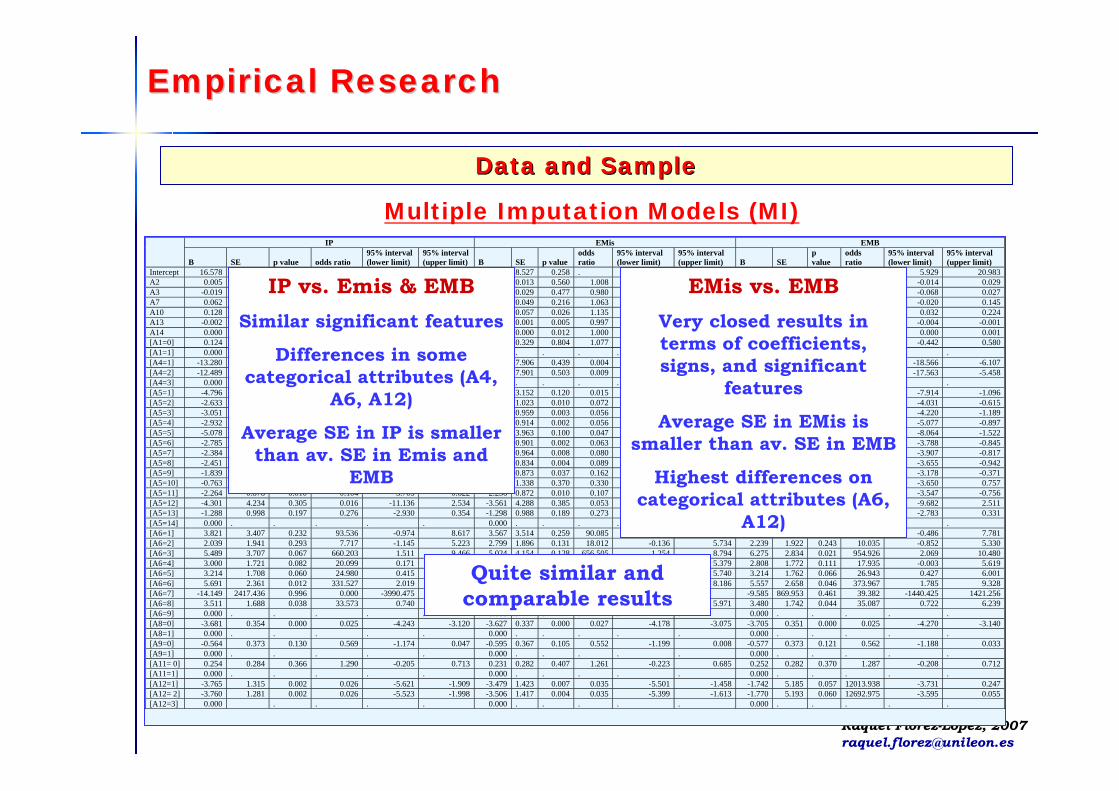
Data Data andand SampleSample
Multiple Imputation Models (MI)IP EMis EMB
B SE p value odds ratio 95% interval (lower limit)
95% interval (upper limit) B SE p value
odds ratio
95% interval (lower limit)
95% interval (upper limit) B SE
p value
odds ratio
95% interval (lower limit)
95% interval (upper limit)
Intercept 16.578 8.083 0.075 9.430 23.727 9.324 8.527 0.258 . -3.859 22.507 13.456 9.826 0.128 5.929 20.983 A2 0.005 0.014 0.710 1.005 -0.017 0.027 0.008 0.013 0.560 1.008 -0.014 0.029 0.008 0.014 0.572 1.008 -0.014 0.029 A3 -0.019 0.029 0.509 0.981 -0.066 0.028 -0.020 0.029 0.477 0.980 -0.067 0.026 -0.020 0.029 0.480 0.980 -0.068 0.027 A7 0.062 0.051 0.220 1.064 -0.020 0.145 0.061 0.049 0.216 1.063 -0.020 0.142 0.062 0.051 0.218 1.064 -0.020 0.145 A10 0.128 0.059 0.029 1.136 0.032 0.223 0.127 0.057 0.026 1.135 0.033 0.220 0.128 0.059 0.028 1.137 0.032 0.224 A13 -0.002 0.001 0.006 0.998 -0.004 -0.001 -0.003 0.001 0.005 0.997 -0.004 -0.001 -0.003 0.001 0.005 0.997 -0.004 -0.001 A14 0.000 0.000 0.006 1.000 0.000 0.001 0.000 0.000 0.012 1.000 0.000 0.001 0.000 0.000 0.007 1.000 0.000 0.001 [A1=0] 0.124 0.308 0.686 1.133 -0.381 0.630 0.071 0.329 0.804 1.077 -0.430 0.572 0.069 0.318 0.803 1.074 -0.442 0.580 [A1=1] 0.000 . . . . . 0.000 . . . . . 0.000 . . . . . [A4=1] -13.280 7.649 0.137 0.000 -18.132 -8.428 -6.058 7.906 0.439 0.004 -18.827 6.711 -12.337 9.584 0.204 0.018 -18.566 -6.107 [A4=2] -12.489 7.561 0.467 0.001 -16.976 -8.002 -5.251 7.901 0.503 0.009 -18.011 7.509 -11.510 9.537 0.367 0.039 -17.563 -5.458 [A4=3] 0.000 . . . . . 0.000 . . . . . 0.000 . . . . . [A5=1] -4.796 3.257 0.122 0.015 -8.959 -0.633 -4.750 3.152 0.120 0.015 -8.940 -0.559 -4.505 2.695 0.086 0.035 -7.914 -1.096 [A5=2] -2.633 1.031 0.011 0.072 -4.328 -0.937 -2.631 1.023 0.010 0.072 -4.307 -0.954 -2.323 1.648 0.042 0.361 -4.031 -0.615 [A5=3] -3.051 0.991 0.002 0.048 -4.633 -1.470 -2.881 0.959 0.003 0.056 -4.448 -1.314 -2.705 1.240 0.040 0.108 -4.220 -1.189 [A5=4] -2.932 0.915 0.001 0.053 -4.436 -1.428 -2.879 0.914 0.002 0.056 -4.376 -1.383 -2.987 1.292 0.056 0.052 -5.077 -0.897 [A5=5] -5.078 3.933 0.080 0.044 -8.342 -1.813 -5.070 3.963 0.100 0.047 -8.299 -1.841 -4.793 3.094 0.070 0.180 -8.064 -1.522 [A5=6] -2.785 0.893 0.002 0.062 -4.252 -1.318 -2.766 0.901 0.002 0.063 -4.224 -1.308 -2.317 1.807 0.005 0.724 -3.788 -0.845 [A5=7] -2.384 0.957 0.012 0.092 -3.947 -0.820 -2.531 0.964 0.008 0.080 -4.093 -0.969 -2.362 1.121 0.039 0.118 -3.907 -0.817 [A5=8] -2.451 0.841 0.004 0.086 -3.832 -1.069 -2.414 0.834 0.004 0.089 -3.785 -1.044 -2.299 0.950 0.014 0.113 -3.655 -0.942 [A5=9] -1.839 0.883 0.036 0.159 -3.281 -0.396 -1.823 0.873 0.037 0.162 -3.255 -0.391 -1.775 0.890 0.040 0.175 -3.178 -0.371 [A5=10] -0.763 1.262 0.545 0.467 -2.832 1.305 -1.157 1.338 0.370 0.330 -3.214 0.901 -1.447 2.123 0.415 0.363 -3.650 0.757 [A5=11] -2.264 0.878 0.010 0.104 -3.705 -0.822 -2.236 0.872 0.010 0.107 -3.668 -0.804 -2.152 0.967 0.018 0.131 -3.547 -0.756 [A5=12] -4.301 4.234 0.305 0.016 -11.136 2.534 -3.561 4.288 0.385 0.053 -9.992 2.870 -3.585 4.073 0.346 0.095 -9.682 2.511 [A5=13] -1.288 0.998 0.197 0.276 -2.930 0.354 -1.298 0.988 0.189 0.273 -2.923 0.326 -1.226 0.992 0.204 0.305 -2.783 0.331 [A5=14] 0.000 . . . . . 0.000 . . . . . 0.000 . . . . . [A6=1] 3.821 3.407 0.232 93.536 -0.974 8.617 3.567 3.514 0.259 90.085 -1.135 8.270 3.648 3.014 0.218 87.665 -0.486 7.781 [A6=2] 2.039 1.941 0.293 7.717 -1.145 5.223 2.799 1.896 0.131 18.012 -0.136 5.734 2.239 1.922 0.243 10.035 -0.852 5.330 [A6=3] 5.489 3.707 0.067 660.203 1.511 9.466 5.024 4.154 0.128 656.505 1.254 8.794 6.275 2.834 0.021 954.926 2.069 10.480 [A6=4] 3.000 1.721 0.082 20.099 0.171 5.829 2.626 1.765 0.125 14.839 -0.128 5.379 2.808 1.772 0.111 17.935 -0.003 5.619 [A6=5] 3.214 1.708 0.060 24.980 0.415 6.012 3.004 1.748 0.077 21.518 0.269 5.740 3.214 1.762 0.066 26.943 0.427 6.001 [A6=6] 5.691 2.361 0.012 331.527 2.019 9.363 4.633 2.730 0.056 161.101 1.080 8.186 5.557 2.658 0.046 373.967 1.785 9.328 [A6=7] -14.149 2417.436 0.996 0.000 -3990.475 3962.177 -15.686 2.529 . . . . -9.585 869.953 0.461 39.382 -1440.425 1421.256 [A6=8] 3.511 1.688 0.038 33.573 0.740 6.281 3.263 1.719 0.052 27.585 0.556 5.971 3.480 1.742 0.044 35.087 0.722 6.239 [A6=9] 0.000 . . . . . 0.000 . . . . . 0.000 . . . . . [A8=0] -3.681 0.354 0.000 0.025 -4.243 -3.120 -3.627 0.337 0.000 0.027 -4.178 -3.075 -3.705 0.351 0.000 0.025 -4.270 -3.140 [A8=1] 0.000 . . . . . 0.000 . . . . . 0.000 . . . . . [A9=0] -0.564 0.373 0.130 0.569 -1.174 0.047 -0.595 0.367 0.105 0.552 -1.199 0.008 -0.577 0.373 0.121 0.562 -1.188 0.033 [A9=1] 0.000 . . . . . 0.000 . . . . . 0.000 . . . . . [A11= 0] 0.254 0.284 0.366 1.290 -0.205 0.713 0.231 0.282 0.407 1.261 -0.223 0.685 0.252 0.282 0.370 1.287 -0.208 0.712 [A11=1] 0.000 . . . . . 0.000 . . . . . 0.000 . . . . . [A12=1] -3.765 1.315 0.002 0.026 -5.621 -1.909 -3.479 1.423 0.007 0.035 -5.501 -1.458 -1.742 5.185 0.057 12013.938 -3.731 0.247 [A12= 2] -3.760 1.281 0.002 0.026 -5.523 -1.998 -3.506 1.417 0.004 0.035 -5.399 -1.613 -1.770 5.193 0.060 12692.975 -3.595 0.055 [A12=3] 0.000 . . . . 0.000 . . . . . 0.000 . . . . .
Raquel Florez-Lopez, [email protected]
Empirical ResearchEmpirical Research
Data Data andand SampleSample
Multiple Imputation Models (MI)IP EMis EMB
B SE p value odds ratio 95% interval (lower limit)
95% interval (upper limit) B SE p value
odds ratio
95% interval (lower limit)
95% interval (upper limit) B SE
p value
odds ratio
95% interval (lower limit)
95% interval (upper limit)
Intercept 16.578 8.083 0.075 9.430 23.727 9.324 8.527 0.258 . -3.859 22.507 13.456 9.826 0.128 5.929 20.983 A2 0.005 0.014 0.710 1.005 -0.017 0.027 0.008 0.013 0.560 1.008 -0.014 0.029 0.008 0.014 0.572 1.008 -0.014 0.029 A3 -0.019 0.029 0.509 0.981 -0.066 0.028 -0.020 0.029 0.477 0.980 -0.067 0.026 -0.020 0.029 0.480 0.980 -0.068 0.027 A7 0.062 0.051 0.220 1.064 -0.020 0.145 0.061 0.049 0.216 1.063 -0.020 0.142 0.062 0.051 0.218 1.064 -0.020 0.145 A10 0.128 0.059 0.029 1.136 0.032 0.223 0.127 0.057 0.026 1.135 0.033 0.220 0.128 0.059 0.028 1.137 0.032 0.224 A13 -0.002 0.001 0.006 0.998 -0.004 -0.001 -0.003 0.001 0.005 0.997 -0.004 -0.001 -0.003 0.001 0.005 0.997 -0.004 -0.001 A14 0.000 0.000 0.006 1.000 0.000 0.001 0.000 0.000 0.012 1.000 0.000 0.001 0.000 0.000 0.007 1.000 0.000 0.001 [A1=0] 0.124 0.308 0.686 1.133 -0.381 0.630 0.071 0.329 0.804 1.077 -0.430 0.572 0.069 0.318 0.803 1.074 -0.442 0.580 [A1=1] 0.000 . . . . . 0.000 . . . . . 0.000 . . . . . [A4=1] -13.280 7.649 0.137 0.000 -18.132 -8.428 -6.058 7.906 0.439 0.004 -18.827 6.711 -12.337 9.584 0.204 0.018 -18.566 -6.107 [A4=2] -12.489 7.561 0.467 0.001 -16.976 -8.002 -5.251 7.901 0.503 0.009 -18.011 7.509 -11.510 9.537 0.367 0.039 -17.563 -5.458 [A4=3] 0.000 . . . . . 0.000 . . . . . 0.000 . . . . . [A5=1] -4.796 3.257 0.122 0.015 -8.959 -0.633 -4.750 3.152 0.120 0.015 -8.940 -0.559 -4.505 2.695 0.086 0.035 -7.914 -1.096 [A5=2] -2.633 1.031 0.011 0.072 -4.328 -0.937 -2.631 1.023 0.010 0.072 -4.307 -0.954 -2.323 1.648 0.042 0.361 -4.031 -0.615 [A5=3] -3.051 0.991 0.002 0.048 -4.633 -1.470 -2.881 0.959 0.003 0.056 -4.448 -1.314 -2.705 1.240 0.040 0.108 -4.220 -1.189 [A5=4] -2.932 0.915 0.001 0.053 -4.436 -1.428 -2.879 0.914 0.002 0.056 -4.376 -1.383 -2.987 1.292 0.056 0.052 -5.077 -0.897 [A5=5] -5.078 3.933 0.080 0.044 -8.342 -1.813 -5.070 3.963 0.100 0.047 -8.299 -1.841 -4.793 3.094 0.070 0.180 -8.064 -1.522 [A5=6] -2.785 0.893 0.002 0.062 -4.252 -1.318 -2.766 0.901 0.002 0.063 -4.224 -1.308 -2.317 1.807 0.005 0.724 -3.788 -0.845 [A5=7] -2.384 0.957 0.012 0.092 -3.947 -0.820 -2.531 0.964 0.008 0.080 -4.093 -0.969 -2.362 1.121 0.039 0.118 -3.907 -0.817 [A5=8] -2.451 0.841 0.004 0.086 -3.832 -1.069 -2.414 0.834 0.004 0.089 -3.785 -1.044 -2.299 0.950 0.014 0.113 -3.655 -0.942 [A5=9] -1.839 0.883 0.036 0.159 -3.281 -0.396 -1.823 0.873 0.037 0.162 -3.255 -0.391 -1.775 0.890 0.040 0.175 -3.178 -0.371 [A5=10] -0.763 1.262 0.545 0.467 -2.832 1.305 -1.157 1.338 0.370 0.330 -3.214 0.901 -1.447 2.123 0.415 0.363 -3.650 0.757 [A5=11] -2.264 0.878 0.010 0.104 -3.705 -0.822 -2.236 0.872 0.010 0.107 -3.668 -0.804 -2.152 0.967 0.018 0.131 -3.547 -0.756 [A5=12] -4.301 4.234 0.305 0.016 -11.136 2.534 -3.561 4.288 0.385 0.053 -9.992 2.870 -3.585 4.073 0.346 0.095 -9.682 2.511 [A5=13] -1.288 0.998 0.197 0.276 -2.930 0.354 -1.298 0.988 0.189 0.273 -2.923 0.326 -1.226 0.992 0.204 0.305 -2.783 0.331 [A5=14] 0.000 . . . . . 0.000 . . . . . 0.000 . . . . . [A6=1] 3.821 3.407 0.232 93.536 -0.974 8.617 3.567 3.514 0.259 90.085 -1.135 8.270 3.648 3.014 0.218 87.665 -0.486 7.781 [A6=2] 2.039 1.941 0.293 7.717 -1.145 5.223 2.799 1.896 0.131 18.012 -0.136 5.734 2.239 1.922 0.243 10.035 -0.852 5.330 [A6=3] 5.489 3.707 0.067 660.203 1.511 9.466 5.024 4.154 0.128 656.505 1.254 8.794 6.275 2.834 0.021 954.926 2.069 10.480 [A6=4] 3.000 1.721 0.082 20.099 0.171 5.829 2.626 1.765 0.125 14.839 -0.128 5.379 2.808 1.772 0.111 17.935 -0.003 5.619 [A6=5] 3.214 1.708 0.060 24.980 0.415 6.012 3.004 1.748 0.077 21.518 0.269 5.740 3.214 1.762 0.066 26.943 0.427 6.001 [A6=6] 5.691 2.361 0.012 331.527 2.019 9.363 4.633 2.730 0.056 161.101 1.080 8.186 5.557 2.658 0.046 373.967 1.785 9.328 [A6=7] -14.149 2417.436 0.996 0.000 -3990.475 3962.177 -15.686 2.529 . . . . -9.585 869.953 0.461 39.382 -1440.425 1421.256 [A6=8] 3.511 1.688 0.038 33.573 0.740 6.281 3.263 1.719 0.052 27.585 0.556 5.971 3.480 1.742 0.044 35.087 0.722 6.239 [A6=9] 0.000 . . . . . 0.000 . . . . . 0.000 . . . . . [A8=0] -3.681 0.354 0.000 0.025 -4.243 -3.120 -3.627 0.337 0.000 0.027 -4.178 -3.075 -3.705 0.351 0.000 0.025 -4.270 -3.140 [A8=1] 0.000 . . . . . 0.000 . . . . . 0.000 . . . . . [A9=0] -0.564 0.373 0.130 0.569 -1.174 0.047 -0.595 0.367 0.105 0.552 -1.199 0.008 -0.577 0.373 0.121 0.562 -1.188 0.033 [A9=1] 0.000 . . . . . 0.000 . . . . . 0.000 . . . . . [A11= 0] 0.254 0.284 0.366 1.290 -0.205 0.713 0.231 0.282 0.407 1.261 -0.223 0.685 0.252 0.282 0.370 1.287 -0.208 0.712 [A11=1] 0.000 . . . . . 0.000 . . . . . 0.000 . . . . . [A12=1] -3.765 1.315 0.002 0.026 -5.621 -1.909 -3.479 1.423 0.007 0.035 -5.501 -1.458 -1.742 5.185 0.057 12013.938 -3.731 0.247 [A12= 2] -3.760 1.281 0.002 0.026 -5.523 -1.998 -3.506 1.417 0.004 0.035 -5.399 -1.613 -1.770 5.193 0.060 12692.975 -3.595 0.055 [A12=3] 0.000 . . . . 0.000 . . . . . 0.000 . . . . .
Quite similar andcomparable results
EMis vs. EMBVery closed results in terms of coefficients, signs, and significant
features
Average SE in EMis issmaller than av. SE in EMB
Highest differences oncategorical attributes (A6,
A12)
IP vs. Emis & EMBSimilar significant features
Differences in somecategorical attributes (A4,
A6, A12)
Average SE in IP is smallerthan av. SE in Emis and
EMB

Raquel Florez-Lopez, [email protected]
Listwise deletion (CC) Mean Substitution (MS)
B SE p value odds ratio 95% interval (lower limit)
95% interval (upper limit) B SE p value
odds ratio
95% interval (lower limit)
95% interval (upper limit) B SE p value
odds ratio
95% interval (lower limit)
95% interval (upper limit)
Intercept -11.052 11.901 0.353 7.322 7.810 0.349 11.946 11.094 0.265 . -1.800 25.693 A2 0.013 0.014 0.356 1.013 -0.015 0.041 0.012 0.013 0.351 1.012 -0.013 0.037 0.005 0.014 0.696 1.005 -0.016 0.026 A3 -0.024 0.030 0.420 0.976 -0.082 0.034 -0.018 0.029 0.542 0.983 -0.074 0.039 -0.019 0.029 0.497 0.981 -0.067 0.028 A7 0.081 0.055 0.146 1.084 -0.028 0.189 0.057 0.049 0.245 1.059 -0.039 0.154 0.063 0.050 0.203 1.066 -0.018 0.145 A10 0.131 0.060 0.029 1.140 0.014 0.248 0.125 0.057 0.029 1.134 0.013 0.238 0.126 0.058 0.028 1.134 0.032 0.220 A13 -0.003 0.001 0.007 0.997 -0.004 -0.001 -0.002 0.001 0.006 0.998 -0.004 -0.001 -0.045 0.120 0.093 0.959 -0.137 0.047 A14 0.001 0.000 0.005 1.001 0.000 0.001 0.000 0.000 0.014 1.000 0.000 0.001 0.000 0.000 0.010 1.000 0.000 0.001 [A1=0] 0.078 0.323 0.810 1.081 -0.556 0.712 0.082 0.308 0.790 1.085 -0.521 0.685 0.074 0.261 0.601 1.079 -0.331 0.478 [A1=1] 0.000 . . . . . 0.000 . . . . . 0.419 13.686 0.878 8.126 -22.027 22.865 [A4=1] -5.635 11.725 0.631 0.004 -28.616 17.345 -4.881 7.526 0.517 0.008 -19.631 9.869 -7.220 11.409 0.428 1.604 -19.358 4.919 [A4=2] -4.790 11.721 0.683 0.008 -27.762 18.182 -4.078 7.519 0.588 0.017 -18.816 10.660 -7.006 9.677 0.480 0.006 -16.428 2.415 [A4=3] 0.000 . . . . . 0.000 . . . . . -1.221 8.432 0.437 0.002 -14.149 11.708 [A5=1] -6.549 2.257 0.004 0.001 -10.973 -2.125 -6.328 2.195 0.004 0.002 -10.630 -2.026 -4.183 3.955 0.225 0.044 -9.733 1.366 [A5=2] -2.004 1.101 0.069 0.135 -4.161 0.153 -2.562 1.032 0.013 0.077 -4.585 -0.539 -2.181 1.705 0.008 0.066 -3.852 -0.510 [A5=3] -3.134 1.007 0.002 0.044 -5.109 -1.160 -2.901 0.966 0.003 0.055 -4.793 -1.008 -3.268 1.629 0.024 0.046 -5.492 -1.043 [A5=4] -3.189 0.964 0.001 0.041 -5.079 -1.300 -2.988 0.923 0.001 0.050 -4.797 -1.179 -2.834 0.961 0.004 0.060 -4.356 -1.312 [A5=5] -7.052 2.365 0.003 0.001 -11.687 -2.416 -6.881 2.311 0.003 0.001 -11.411 -2.351 -4.212 2.702 0.059 0.030 -7.253 -1.171 [A5=6] -2.790 0.931 0.003 0.061 -4.615 -0.966 -2.748 0.897 0.002 0.064 -4.507 -0.989 -2.710 0.903 0.002 0.067 -4.173 -1.248 [A5=7] -2.599 0.994 0.009 0.074 -4.548 -0.650 -2.441 0.961 0.011 0.087 -4.325 -0.557 -2.702 1.250 0.018 0.073 -4.554 -0.851 [A5=8] -2.478 0.878 0.005 0.084 -4.198 -0.758 -2.423 0.843 0.004 0.089 -4.076 -0.770 -2.402 0.866 0.005 0.092 -3.787 -1.017 [A5=9] -1.880 0.914 0.040 0.153 -3.672 -0.089 -1.779 0.881 0.043 0.169 -3.506 -0.053 -1.913 0.953 0.035 0.153 -3.369 -0.456 [A5=10] -0.712 1.358 0.600 0.491 -3.373 1.950 -0.806 1.269 0.525 0.447 -3.294 1.681 -1.367 1.360 0.307 0.289 -3.278 0.544 [A5=11] -2.471 0.916 0.007 0.084 -4.267 -0.676 -2.259 0.880 0.010 0.104 -3.984 -0.533 -2.135 0.901 0.017 0.121 -3.564 -0.706 [A5=12] -4.674 4.446 0.293 0.009 -13.389 4.040 -5.003 4.149 0.228 0.007 -13.135 3.129 -2.610 3.441 0.417 0.140 -7.732 2.512 [A5=13] -1.360 1.037 0.190 0.257 -3.393 0.673 -1.279 1.000 0.201 0.278 -3.238 0.681 -1.466 1.093 0.164 0.247 -3.053 0.120 [A5=14] 0.000 . . . . . 0.000 . . . . . -0.595 4.375 0.470 0.051 -7.362 6.172 [A6=1] 5.890 2.653 0.026 361.533 0.690 11.091 -3.670 0.341 0.000 0.025 -4.339 -3.001 1.848 3.603 0.374 40.376 -1.866 5.563 [A6=2] 2.598 1.985 0.191 13.433 -1.294 6.489 0.000 . . . . . 2.081 2.241 0.154 14.086 -0.867 5.028 [A6=3] 7.976 2.785 0.004 2911.544 2.518 13.435 -0.620 0.369 0.093 0.538 -1.343 0.103 4.584 3.245 0.123 387.712 0.379 8.789 [A6=4] 3.553 1.824 0.051 34.910 -0.023 7.128 0.000 . . . . . 2.530 1.753 0.148 13.019 -0.299 5.359 [A6=5] 3.843 1.793 0.032 46.688 0.330 7.357 0.270 0.279 0.333 1.310 -0.277 0.816 3.310 2.066 0.073 41.191 0.335 6.285 [A6=6] 6.748 2.386 0.005 852.140 2.072 11.423 0.000 . . . . . 4.366 2.344 0.042 112.837 0.989 7.743 [A6=7] -11.478 7128.257 0.999 0.000 . . -3.348 0.971 0.001 0.035 -5.252 -1.444 -11.795 963.142 0.526 4.865 -1595.945 1572.354 [A6=8] 4.060 1.775 0.022 57.957 0.582 7.538 -3.302 0.894 0.000 0.037 -5.053 -1.550 3.415 1.834 0.052 34.015 0.539 6.290 [A6=9] 0.000 . . . . . 0.000 . . . . . -3.178 7.946 . 0.000 . . [A8=0] -3.836 0.363 0.000 0.022 -4.547 -3.124 5.384 2.545 0.034 217.837 0.396 10.371 -2.197 3.618 0.006 6.717 -3.177 -1.216 [A8=1] 0.000 . . . . . 2.400 1.908 0.208 11.021 -1.339 6.139 0.000 0.000 . . . . [A9=0] -0.417 0.382 0.275 0.659 -1.165 0.332 7.595 2.672 0.004 1988.075 2.357 12.833 -1.192 1.534 0.085 0.447 -1.785 -0.599 [A9=1] 0.000 . . . . . 3.079 1.687 0.068 21.734 -0.228 6.385 0.000 0.000 . . . . [A11= 0] 0.242 0.289 0.401 1.274 -0.323 0.808 3.474 1.670 0.037 32.280 0.201 6.748 0.063 0.531 0.329 1.123 -0.420 0.546 [A11=1] 0.000 . . . . . 6.285 2.276 0.006 536.540 1.824 10.746 0.000 0.000 . . . . [A12=1] 15.312 0.513 0.000 4467302.058 14.307 16.317 -13.627 0.000 . 0.000 -13.627 -13.627 -3.650 1.203 0.003 0.028 -5.493 -1.807 [A12= 2] 15.407 0.000 . 4912834.337 15.407 15.407 3.729 1.653 0.024 41.651 0.490 6.968 -3.704 1.120 0.001 0.026 -5.431 -1.978 [A12=3] 0.000 . . . -0.015 0.041 0.000 . . . . . 0.000 0.000 . . . .
Empirical ResearchEmpirical Research
Data Data andand SampleSample
Listwise deletion, mean/median substitution, EM algorithm
EM algorithmNear to EMis results (signs,
significant features)
Estimates and av. SE are larger, pointing a higherinstability of coefficients
Listwise deletion (CC)Quite different than other
models (categoricalattributes A5, A6, A8,
A12): Possible bias
Estimates and av. SE are larger than other methods, as expected (Ibrahin et al,
2005)
Mean/median Substit.Quite different than other
models (categoricalattributes A6, A8, A12):
Possible bias
It obtains the highestnumber of statistically
significant features
Very wide 95% confidenceintervals: high uncertainty
in estimates

Raquel Florez-Lopez, [email protected]
Empirical ResearchEmpirical Research
Data Data andand SampleSample
Error estimates (in-sample)
49.60 (12.95%)30.40 (9.90%)80.00 (11.59%)EMB50.33 (13.14%)30.00 (9.77%)80.33 (11.64%)EMis52.00 (13.58%)30.67 (9.99%)82.67 (11.98%)IP50.20 (13.10%)30.20 (9.84%)80.40 (11.65%)EM53.00 (13.84%)29.00 (9.45%)82.00 (11.88%)MS52.00 (13.58%)32.00 (10.42%)84.00 (12.17%)CCType II errorType I errorOverall errorMethod
Emis and EMB: the most accurate techniques (hit ratio)
EMis and EMB: the most balanced results (type I and II errors)
EM algorithm: Performed quite well, maybe biased parameters
Listwise deletion: Highest error rates
Mean subsitution and IP algorithm: Only partial solutions

Raquel Florez-Lopez, [email protected]
AgendaAgenda
1. Introduction
2. Effects of missing data in credit risk scoring. A LDP perspective4.1. Managing sparce default records and missing data
4.2. The case of Low Default Portfolios (LDPs)
3. Dealing with missing values. A methodological analysis
4. Empirical research. The Australian credit approval dataset
5. Conclusions and remarks

Raquel Florez-Lopez, [email protected]
ConclusionsConclusions
- Internal default experience is used to estimate PD in IRB systems.
- An extensive database is necessary to get statistical validation, but in practiceinternal datasets are usually incomplete or do not contain enough history forestimating PD.
- To improve data quality and consistence, several methods can be applied tohandle missing values (six categories): listwise deletion, substitutionapproaches, maximum likelihood, multiple imputation, weighting methods, fully Bayesian approaches.
- The presence of missing values is more critical in presence of sparce-data portfolios and could case average observed default rates not be statisticallyreliable estimators of PD for IRB systems.

Raquel Florez-Lopez, [email protected]
ConclusionsConclusions
- No theoretical rules are provided about the best approach to be used, but itdepends on the missing data nature. Listwise deletion is profusely appliedbut generates accuracy and bias problems.
- In this paper, we analyse the nature of missing data, together torobustness, stability, bias and accuracy of six methods for sparce data credit risk portfolios.
- Results show that maximum likelihood and multiple imputationapproaches obtain promising accurate results, unbiased parameters, androbust models.

Raquel Florez-Lopez, [email protected]
“Effects of missing data in credit risk scoring. A comparative analysis of methods to gain robustness in presence of sparce data”
Raquel Flórez-LópezDepartment of Economics and Business Administration
University of León (SPAIN)
CreditCredit ResearchResearch CentreCentreCreditCredit ScoringScoring andand CreditCredit Control XControl X
29-31 August 2007The University of Edinburgh - Management School