Embed Size (px)
Citation preview

University of HoustonIMAQS
Effects of Land Cover Changes on the Air Quality in the
Houston-Galveston Area
Daewon W. ByunUniversity of Houston
Institute for Multidimensional Air Quality Studies (IMAQS)
University of HoustonIMAQS
Research TeamUniversity of Houston (Daewon Byun)
GEM (Stephen Stetson)TCEQ (Mark Estes)
USDA (David Nowak)SJSU (Bob Bornstein)
Project support HARC (sponsor)
TCEQ, TFS (Pete Smith) USDA (Warren Heilman; John Hom)
EPA (Eva Wong, Brian Timin, J. Edwards, S.T. Rao)

University of HoustonIMAQS
Objectives: Study of the effects of land use and land cover modification on the urban heat island development and on the air quality in the Houston-Galveston metropolitan area.
Methods: Conduct meteorological, emissions, and air quality sensitivity modeling using …•Improve land surface parameterizations with better physics•Incorporate most up-to-dated detailed land use & land cover data for biogenic emissions estimates and meteorological simulations•Perform sensitivity air quality simulations with different emissions & meteorology inputs
University of HoustonIMAQS
Urbanization modeling
• Effects of Land use and Land Cover (LU/LC) changes
• Urban Heat Island (UHI)• Neighborhood Scale Meteorology• Air Quality
University of HoustonIMAQS
How Does the Land Use/Land Cover Change Affect Local Weather/Climate?
• Climate is a cumulative state of local weather• There are synoptic changes in the weather due
to the changes in land surface processes
• More importantly, mesoscale (of the scale 100s – 1000s km) and neighborhood scale (of the scale 1s – 10s km) meteorology is dependent on the changes in the local energy budget and surface characteristics more closely
University of HoustonIMAQS
How does the Land Use/Land Cover Change Affect Local Weather/Climate?• Land surface changes affect the thermal and
radiative characteristics of the energy balance
• The diurnal evolution of heat (temp.) and momentum (winds) in the planetary boundary layer (PBL) is strongly affected by the energy balance and moisture budget.
University of HoustonIMAQS
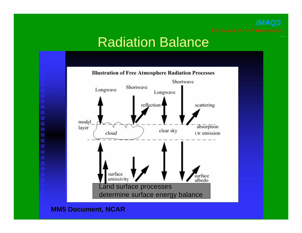
Radiation Balance
MM5 Document, NCAR
Land surface processes determine surface energy balance
University of HoustonIMAQS
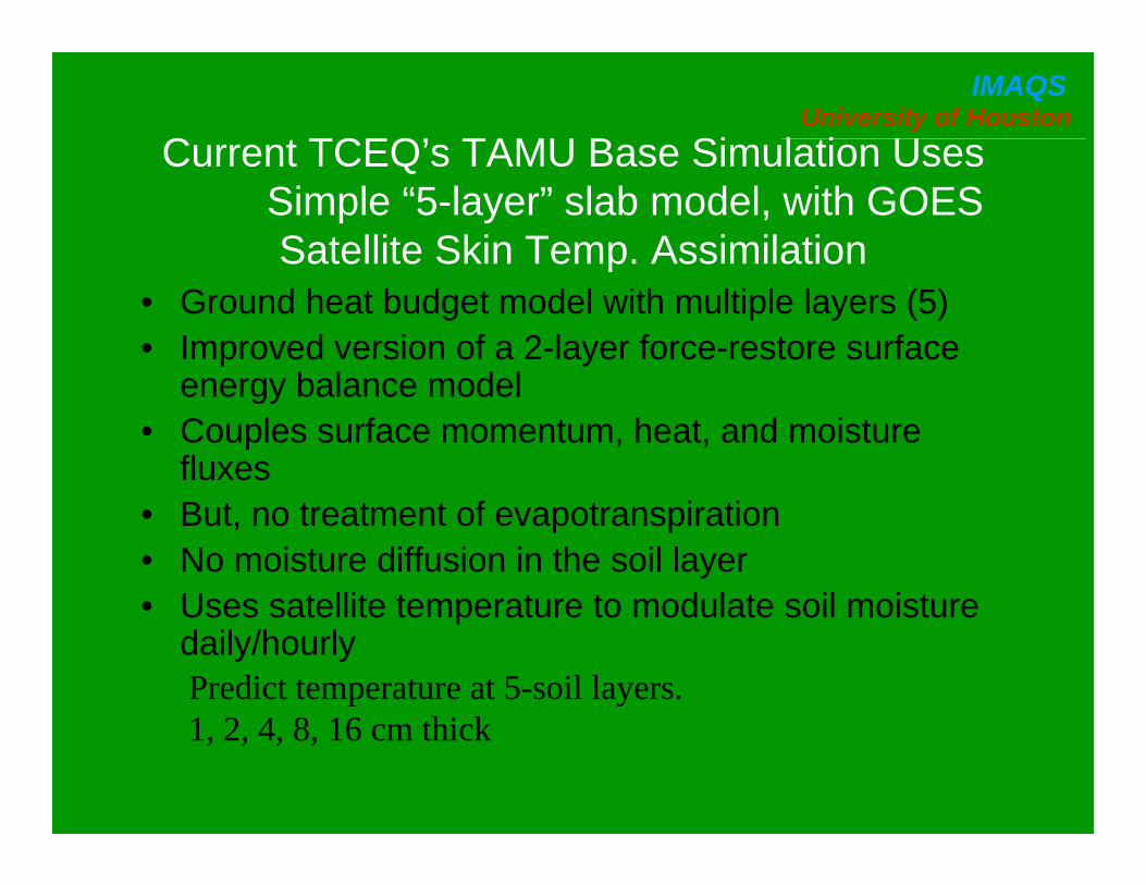
• Ground heat budget model with multiple layers (5)• Improved version of a 2-layer force-restore surface
energy balance model• Couples surface momentum, heat, and moisture
fluxes• But, no treatment of evapotranspiration• No moisture diffusion in the soil layer• Uses satellite temperature to modulate soil moisture
daily/hourlyPredict temperature at 5-soil layers.1, 2, 4, 8, 16 cm thick
Current TCEQ’s TAMU Base Simulation UsesSimple “5-layer” slab model, with GOES Satellite Skin Temp. Assimilation

University of HoustonIMAQS
5-layer slab modelMM5 Document, NCAR
University of HoustonIMAQS
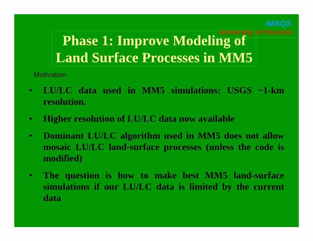
• LU/LC data used in MM5 simulations: USGS ~1-km resolution.
• Higher resolution of LU/LC data now available
• Dominant LU/LC algorithm used in MM5 does not allow mosaic LU/LC land-surface processes (unless the code is modified)
• The question is how to make best MM5 land-surface simulations if our LU/LC data is limited by the current data
Phase 1: Improve Modeling of Land Surface Processes in MM5
Motivation
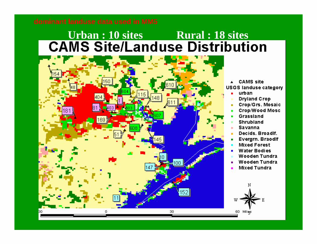
Urban : 10 sites Rural : 18 sitesdominant landuse data used in MM5

University of HoustonIMAQS
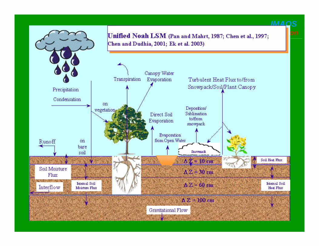
How to better model the land-surface processes?
• Use comprehensive land-surface model• NOAH LSM (N:National Center for
Environmental Prediction; O: Oregon State University; A: Air Force; H: Hydrological Research Lab.) (Ek et al., 2001).
• 4-layers (10, 30, 60, and 100 cm thick)• Predicts soil temperature, soil water, canopy
water, and snow/ice
University of HoustonIMAQS

University of HoustonIMAQSConfiguration of MM5 simulations
• Analysis nudging for d1,d2,d3; observation nudging(wind vector)for d4
• d1, d2 2way nesting; d3,d4 continuous one-way nesting
• MRF PBL Parameterization • Dudhia explicit moisture scheme • RRTM radiation scheme• Slab land-surface model (LSM)
D2D3
D4
D1
4344443121234336362431081081ZY (km)X (km)Domain
Simulation time: Aug. 22~Sep.02, 2000
D4
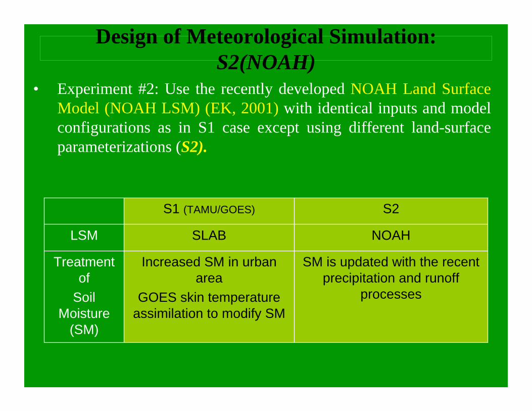
Design of Meteorological Simulation: S2(NOAH)
• Experiment #2: Use the recently developed NOAH Land Surface Model (NOAH LSM) (EK, 2001) with identical inputs and model configurations as in S1 case except using different land-surface parameterizations (S2).
SM is updated with the recent precipitation and runoff
processes
Increased SM in urban area
GOES skin temperature assimilation to modify SM
Treatment of
Soil Moisture
(SM)
NOAHSLABLSM
S2S1 (TAMU/GOES)

Scattered Diagram of 2-m Temp2-m Temperature (S2--NOAH LSM)(Aug.29~31)
Observed (oC)20 25 30 35 40 45 50
Sim
ulat
ion
(S2)
20
25
30
35
40
45
50s152(urban)s100(urban)s115(urban)s181(urban)s167(urban)s404(urban)s169(urban)s81(urban)s1(urban)s403(urban)s11s610s611s147s10s150s154s148s145s410s48s603s604s607s608
Scattered diagram of 2-m temperature with MM5/NOAH simulations.
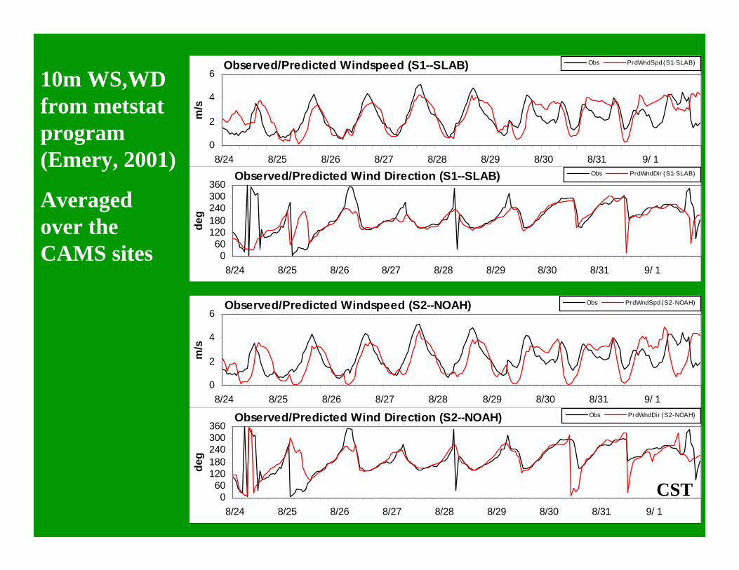
Observed/Predicted Windspeed (S1--SLAB)
0
2
4
6
8/24 8/25 8/26 8/27 8/28 8/29 8/30 8/31 9/ 1
m/s
Obs PrdWndSpd (S1-SLAB)
Observed/Predicted Wind Direction (S1--SLAB)
060
120180240300360
8/24 8/25 8/26 8/27 8/28 8/29 8/30 8/31 9/ 1
deg
Obs PrdWndDir (S1-SLAB)
Observed/Predicted Windspeed (S2--NOAH)
0
2
4
6
8/24 8/25 8/26 8/27 8/28 8/29 8/30 8/31 9/ 1
m/s
Obs PrdWndSpd (S2-NOAH)
Observed/Predicted Wind Direction (S2--NOAH)
060
120180240300360
8/24 8/25 8/26 8/27 8/28 8/29 8/30 8/31 9/ 1
deg
Obs PrdWndDir (S2-NOAH)
CST
10m WS,WD from metstat program (Emery, 2001)
Averaged over the CAMS sites
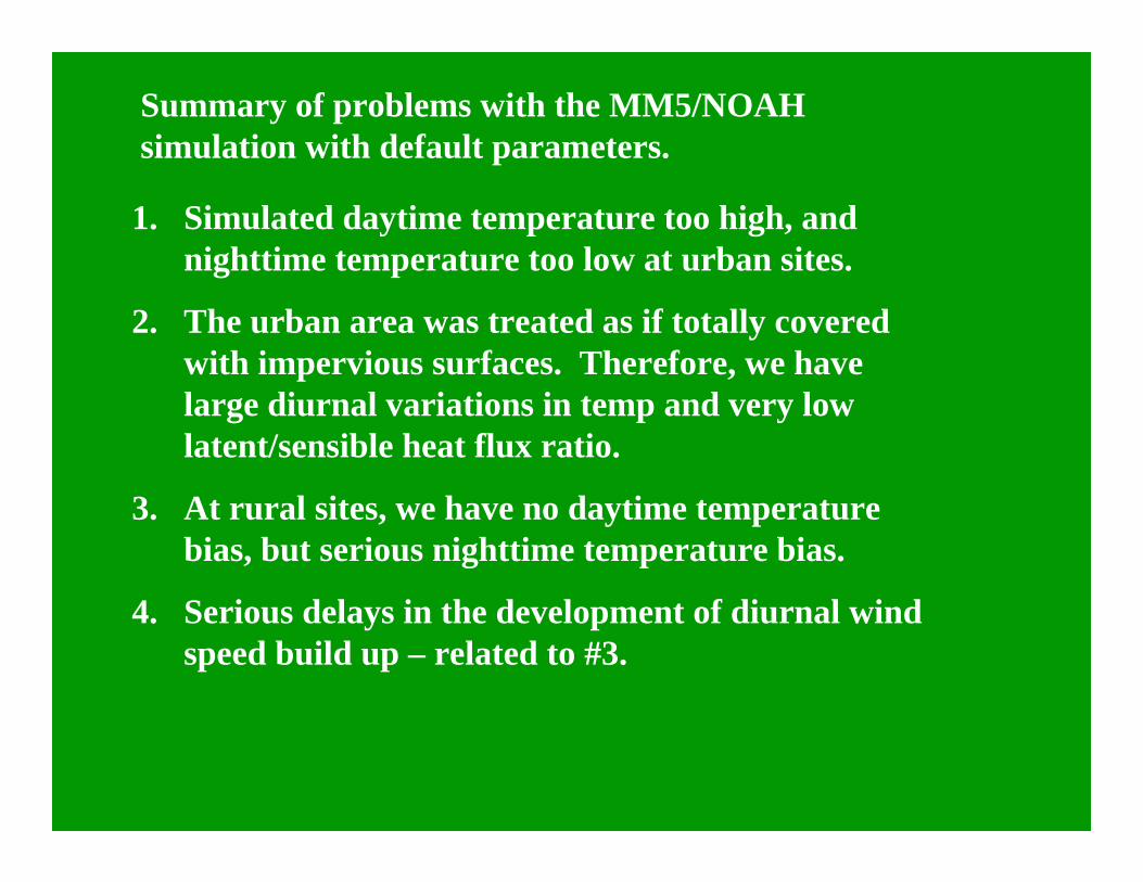
Summary of problems with the MM5/NOAH simulation with default parameters.
1. Simulated daytime temperature too high, and nighttime temperature too low at urban sites.
2. The urban area was treated as if totally covered with impervious surfaces. Therefore, we have large diurnal variations in temp and very low latent/sensible heat flux ratio.
3. At rural sites, we have no daytime temperature bias, but serious nighttime temperature bias.
4. Serious delays in the development of diurnal wind speed build up – related to #3.
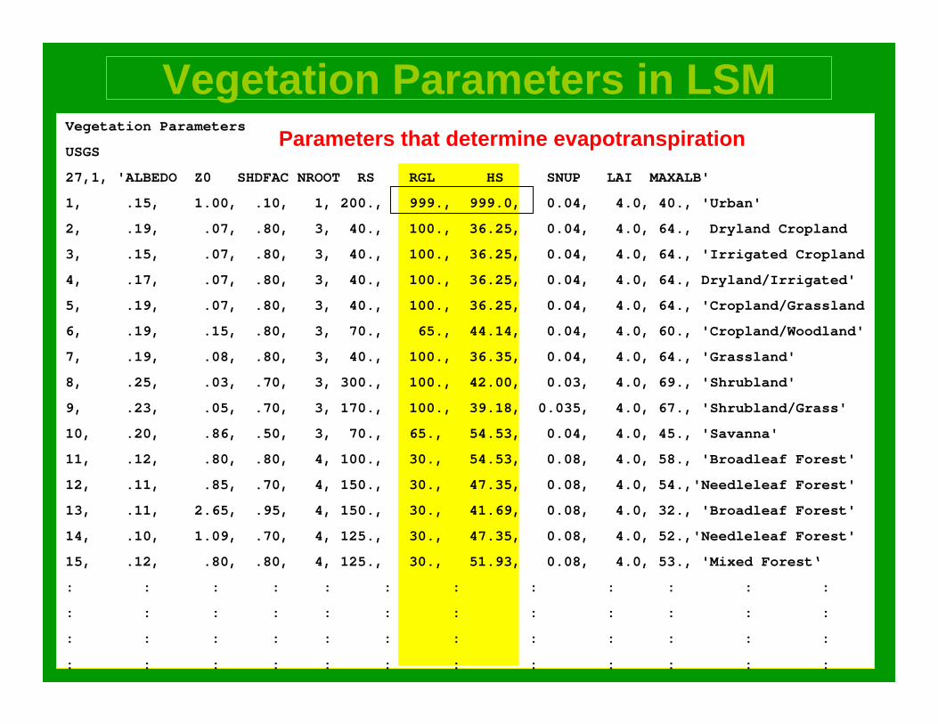
Vegetation Parameters in LSMVegetation Parameters
USGS
27,1, 'ALBEDO Z0 SHDFAC NROOT RS RGL HS SNUP LAI MAXALB'
1, .15, 1.00, .10, 1, 200., 999., 999.0, 0.04, 4.0, 40., 'Urban'
2, .19, .07, .80, 3, 40., 100., 36.25, 0.04, 4.0, 64., Dryland Cropland
3, .15, .07, .80, 3, 40., 100., 36.25, 0.04, 4.0, 64., 'Irrigated Cropland
4, .17, .07, .80, 3, 40., 100., 36.25, 0.04, 4.0, 64., Dryland/Irrigated'
5, .19, .07, .80, 3, 40., 100., 36.25, 0.04, 4.0, 64., 'Cropland/Grassland
6, .19, .15, .80, 3, 70., 65., 44.14, 0.04, 4.0, 60., 'Cropland/Woodland'
7, .19, .08, .80, 3, 40., 100., 36.35, 0.04, 4.0, 64., 'Grassland'
8, .25, .03, .70, 3, 300., 100., 42.00, 0.03, 4.0, 69., 'Shrubland'
9, .23, .05, .70, 3, 170., 100., 39.18, 0.035, 4.0, 67., 'Shrubland/Grass'
10, .20, .86, .50, 3, 70., 65., 54.53, 0.04, 4.0, 45., 'Savanna'
11, .12, .80, .80, 4, 100., 30., 54.53, 0.08, 4.0, 58., 'Broadleaf Forest'
12, .11, .85, .70, 4, 150., 30., 47.35, 0.08, 4.0, 54.,'Needleleaf Forest'
13, .11, 2.65, .95, 4, 150., 30., 41.69, 0.08, 4.0, 32., 'Broadleaf Forest'
14, .10, 1.09, .70, 4, 125., 30., 47.35, 0.08, 4.0, 52.,'Needleleaf Forest'
15, .12, .80, .80, 4, 125., 30., 51.93, 0.08, 4.0, 53., 'Mixed Forest‘
: : : : : : : : : : : :
: : : : : : : : : : : :
: : : : : : : : : : : :
: : : : : : : : : : : :
Parameters that determine evapotranspiration

Addition of Canopy Moisture
is intercepted canopy water content
is green vegetation fraction
is input total precipitation
canopy evaporation
If exceeds S (maximum canopy capacity: 0.5 mm), the excess precipitation or drip, reaches the ground.
ucfc EEDP
tW
+−−=∂∂
σ
cW
fσ
P
cE
cWD
uE is the anthropogenic contribution to the canopy water content. A reasonable value 3x10⁻⁶ (meter of available water per second) was picked for the simulation (* need to be justified).
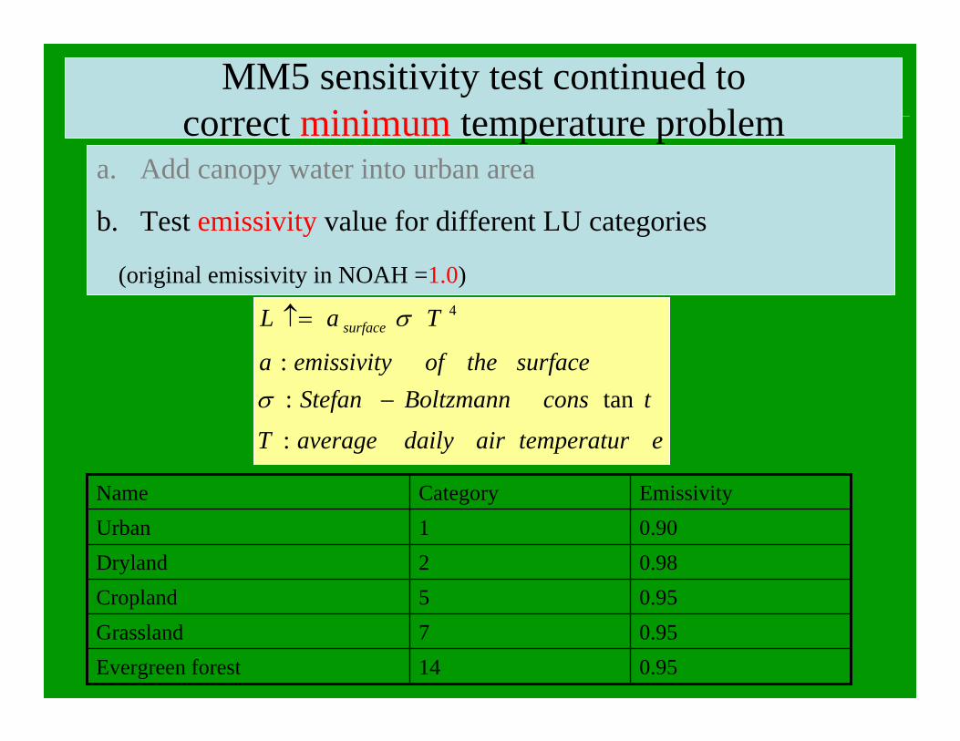
University of HoustonIMAQSMM5 sensitivity test continued to
correct minimum temperature problema. Add canopy water into urban area
b. Test emissivity value for different LU categories
(original emissivity in NOAH =1.0)
etemperaturairdailyaverageT
tconsBoltzmannStefansurfacetheofemissivitya
TaL surface
:
tan::
4
−
↑=
σ
σ
0.955Cropland0.982Dryland
0.9514Evergreen forest0.957Grassland
0.901UrbanEmissivityCategoryName

University of HoustonIMAQS
2-m temperature
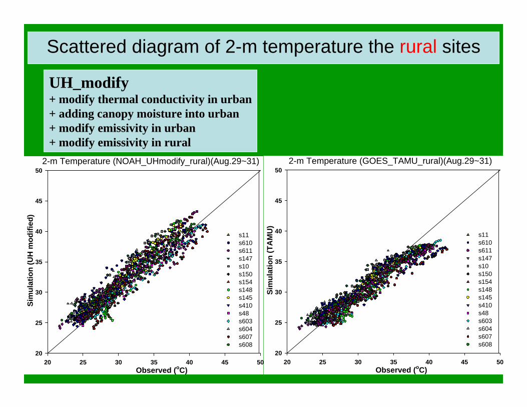
UH_modify+ modify thermal conductivity in urba+ adding canopy moisture into urban+ modify emissivity in urban+ modify emissivity in rural
15
20
25
30
35
40
45
82500 82512 82600 82612 82700 82712 82800 82812 82900 82912 83000 83012 83100 83112
(c)
urban_avg GOES NOAH_fei UH_modify
Urban CAMS site average
15
20
25
30
35
40
45
82500 82512 82600 82612 82700 82712 82800 82812 82900 82912 83000 83012 83100 83112
(c)
rural_avg GOES NOAH_fei UH_modify
Rural CAMS site average
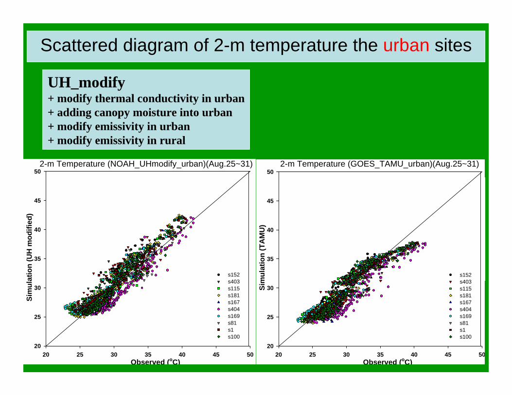
University of HoustonIMAQSScattered diagram of 2-m temperature the urban sites
A consistent low bias in the urban sites especially in s404 (in the boundary of urban and rural area) and s100 (close to coast area).
2-m Temperature (NOAH_UHmodify_urban)(Aug.25~31)
Observed (oC)20 25 30 35 40 45 50
Sim
ulat
ion
(UH
mod
ified
)
20
25
30
35
40
45
50
s152s403s115s181s167s404s169s81s1s100
2-m Temperature (GOES_TAMU_urban)(Aug.25~31)
Observed (oC)20 25 30 35 40 45 50
Sim
ulat
ion
(TA
MU
)
20
25
30
35
40
45
50
s152s403s115s181s167s404s169s81s1s100
UH_modify+ modify thermal conductivity in urban+ adding canopy moisture into urban+ modify emissivity in urban+ modify emissivity in rural
University of HoustonIMAQS
2-m Temperature (GOES_TAMU_rural)(Aug.29~31)
Observed (oC)20 25 30 35 40 45 50
Sim
ulat
ion
(TA
MU
)
20
25
30
35
40
45
50
s11s610s611s147s10s150s154s148s145s410s48s603s604s607s608
2-m Temperature (NOAH_UHmodify_rural)(Aug.29~31)
Observed (oC)20 25 30 35 40 45 50
Sim
ulat
ion
(UH
mod
ified
)
20
25
30
35
40
45
50
s11s610s611s147s10s150s154s148s145s410s48s603s604s607s608
Scattered diagram of 2-m temperature the rural sites
UH_modify+ modify thermal conductivity in urban+ adding canopy moisture into urban+ modify emissivity in urban+ modify emissivity in rural

Observed/Predicted Wind Direction (S1--SLAB)
060
120180240300360
8/24 8/25 8/26 8/27 8/28 8/29 8/30 8/31 9/ 1
deg
Obs PrdWndDir (S1-SLAB)
Observed/Predicted Wind Direction (S2--NOAH)
060
120180240300360
8/24 8/25 8/26 8/27 8/28 8/29 8/30 8/31 9/ 1
deg
Obs PrdWndDir (S2-NOAH)
10m Wind Direction from S1, S2 and S3 simulations:
Observed/Predicted Wind Direction (S3--NOAH_CM)
060
120180240300360
8/24 8/25 8/26 8/27 8/28 8/29 8/30 8/31 9/ 1
deg
ObsWndDir PrdWndDir
CST
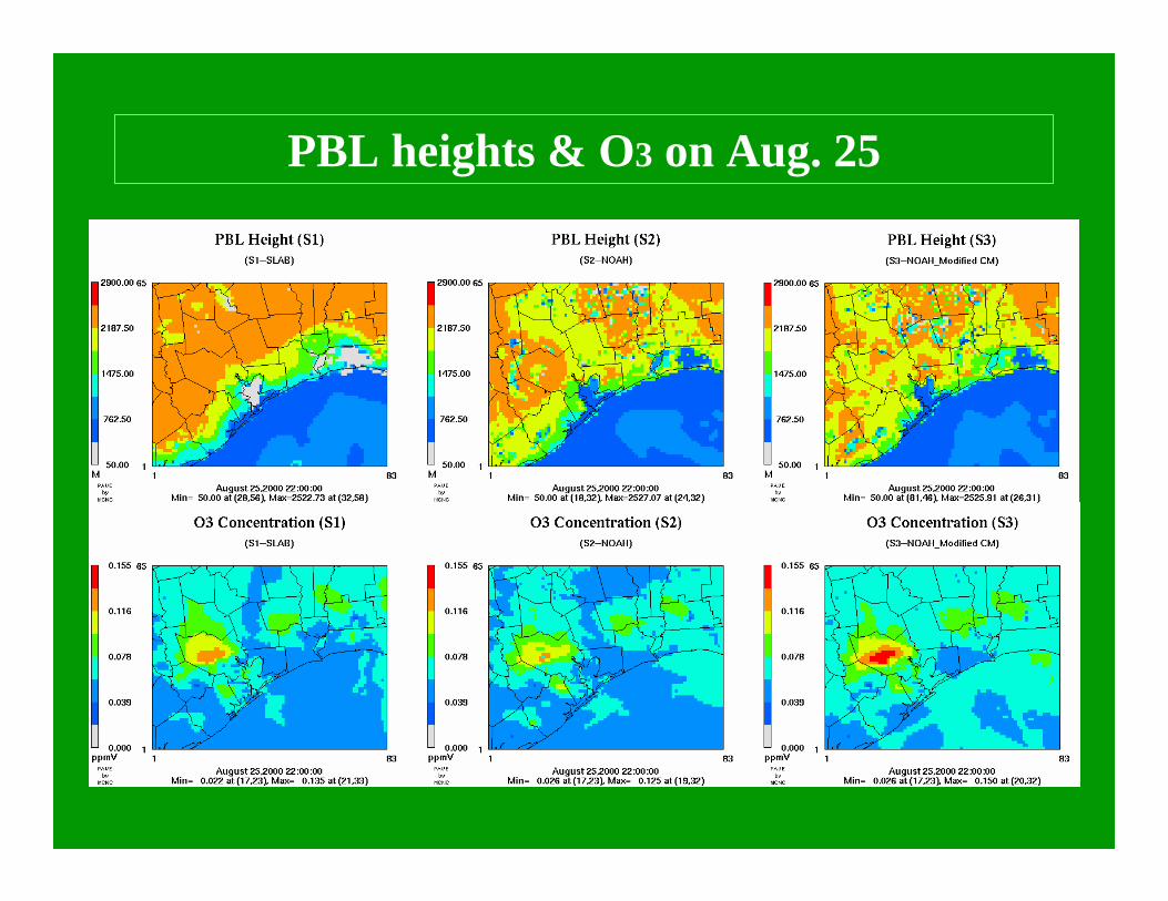
PBL heights & O3 on Aug. 25

Wind Profiler Sites (TexAQS-2000)

PBL Height Analysis from S1, S2 and S3 simulations on Aug. 25Profiler PBL ht. from NOAA/FSL
CST
S3_Aug. 25 PBl ht(m)
0
500
1000
1500
2000
2500
3000
3500
8:00 10:00 12:00 14:00 16:00 18:0
LM EL HS WH LBLMp Elp HSp WHp LBp
S2_Aug. 25 PBl ht(m)
0
500
1000
1500
2000
2500
3000
3500
8:00 10:00 12:00 14:00 16:00 18:00
LM EL HS WH LBLMp Elp HSp WHp LBp
S1_Aug. 25 PBl ht(m)
0
500
1000
1500
2000
2500
3000
3500
8:00 10:00 12:00 14:00 16:00 18:00
LM EL HS WH LBLMp Elp HSp WHp LBp
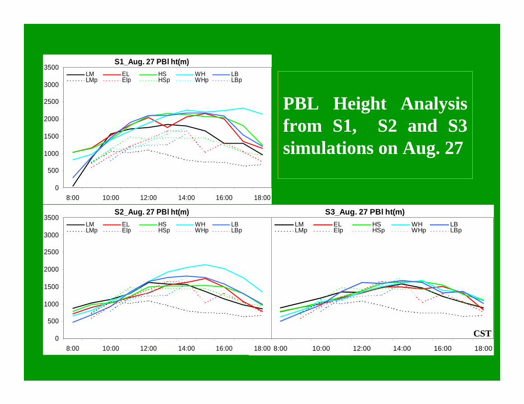
S1_Aug. 27 PBl ht(m)
0
500
1000
1500
2000
2500
3000
3500
8:00 10:00 12:00 14:00 16:00 18:00
LM EL HS WH LBLMp Elp HSp WHp LBp
PBL Height Analysis from S1, S2 and S3 simulations on Aug. 27
S3_Aug. 27 PBl ht(m)
0
500
1000
1500
2000
2500
3000
3500
8:00 10:00 12:00 14:00 16:00 18:00
LM EL HS WH LBLMp Elp HSp WHp LBp
S2_Aug. 27 PBl ht(m)
0
500
1000
1500
2000
2500
3000
3500
8:00 10:00 12:00 14:00 16:00 18:00
LM EL HS WH LBLMp Elp HSp WHp LBp
CST
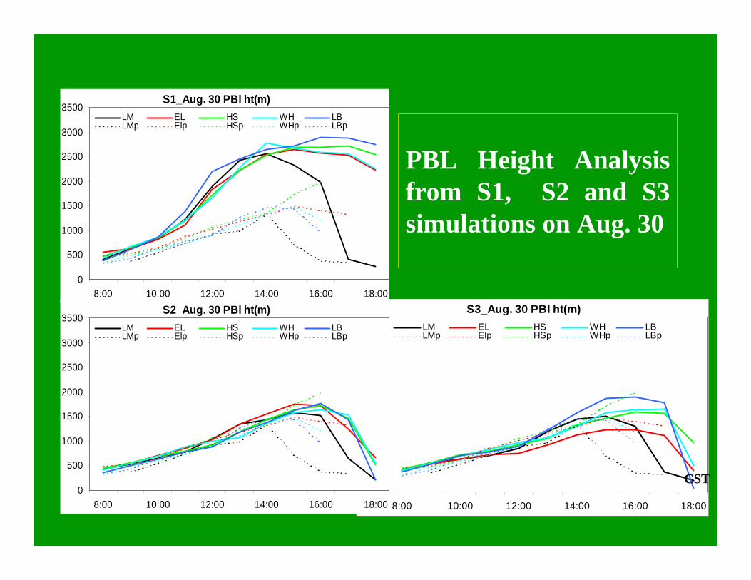
S1_Aug. 30 PBl ht(m)
0
500
1000
1500
2000
2500
3000
3500
8:00 10:00 12:00 14:00 16:00 18:00
LM EL HS WH LBLMp Elp HSp WHp LBp
PBL Height Analysis from S1, S2 and S3 simulations on Aug. 30
S3_Aug. 30 PBl ht(m)
0
500
1000
1500
2000
2500
3000
3500
8:00 10:00 12:00 14:00 16:00 18:00
LM EL HS WH LBLMp Elp HSp WHp LBp
S2_Aug. 30 PBl ht(m)
0
500
1000
1500
2000
2500
3000
3500
8:00 10:00 12:00 14:00 16:00 18:00
LM EL HS WH LBLMp Elp HSp WHp LBp
CST
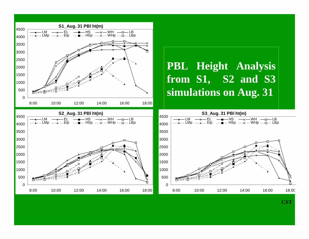
PBL Height Analysis from S1, S2 and S3 simulations on Aug. 31
CST
S1_Aug. 31 PBl ht(m)
0
500
1000
1500
2000
2500
3000
3500
4000
4500
8:00 10:00 12:00 14:00 16:00 18:00
LM EL HS WH LBLMp Elp HSp WHp LBp
S2_Aug. 31 PBl ht(m)
0
500
1000
1500
2000
2500
3000
3500
4000
4500
8:00 10:00 12:00 14:00 16:00 18:00
LM EL HS WH LBLMp Elp HSp WHp LBp
S3_Aug. 31 PBl ht(m)
0
500
1000
1500
2000
2500
3000
3500
4000
4500
8:00 10:00 12:00 14:00 16:00 18:00
LM EL HS WH LBLMp Elp HSp WHp LBp

Summary of Phase 1 MM5/NOAH simulation with
1. Urban area was treated as if it were totally covered with impervious surface. Therefore, we have large diurnal variations in temp and very low latent/sensible heat flux ratio in urban areas.
2. Bias in daytime temperature fixed with added canopy water.
3. The nighttime min. temperature bias was minimized by introducing LU/LC dependent emissivity
4. Still there are serious delays in the development of daytime wind speed build up.

Phase 2: MM5 simulations with LANDSAT derived high-resolution LU/LC
• Continue to test MM5/NOAH with new LANDSAT derived land use and land cover data
• Estimate biogenic emissions with LC and meteorology data
• Study effects on air quality
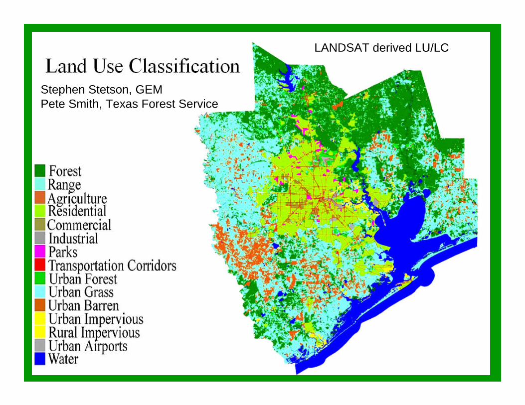
Stephen Stetson, GEMPete Smith, Texas Forest Service
LANDSAT derived LU/LC

Stephen Stetson, GEMPete Smith, Texas Forest Service
LANDSAT derived LU/LC

University of HoustonIMAQS
Digitized for MM5 4-km domain
University of HoustonIMAQS
20
25
30
35
40
45
82500 82600 82700 82800 82900 83000 83100
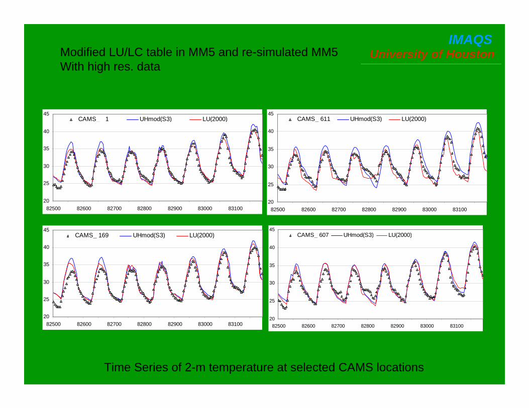
CAMS_ 1 UHmod(S3) LU(2000)
20
25
30
35
40
45
82500 82600 82700 82800 82900 83000 83100
CAMS_ 169 UHmod(S3) LU(2000)
20
25
30
35
40
45
82500 82600 82700 82800 82900 83000 83100
CAMS_ 611 UHmod(S3) LU(2000)
20
25
30
35
40
45
82500 82600 82700 82800 82900 83000 83100
CAMS_ 607 UHmod(S3) LU(2000)
Time Series of 2-m temperature at selected CAMS locations
Modified LU/LC table in MM5 and re-simulated MM5With high res. data

University of HoustonIMAQS
Land cover changes from 1990 overlaid on LADNSAT(Stephen Stetson)
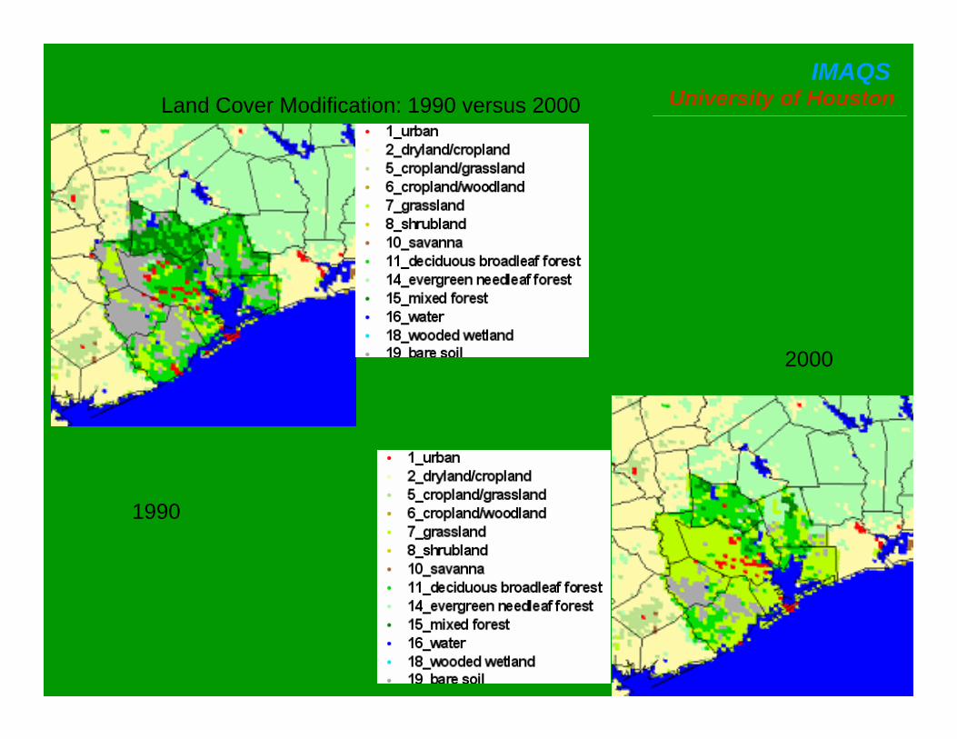
Study effects of land use change on air quality
University of HoustonIMAQS
Land Cover Modification: 1990 versus 2000
1990
2000
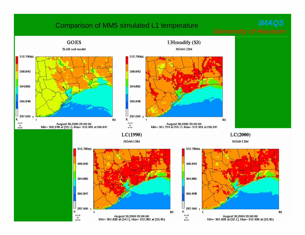
University of HoustonIMAQSComparison of MM5 simulated L1 temperature
University of HoustonIMAQS
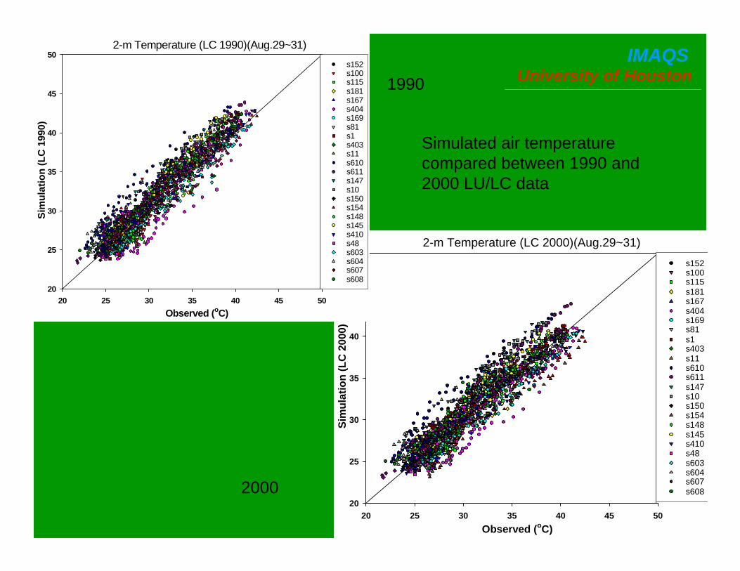
Simulated air temperature compared between 1990 and 2000 LU/LC data
2-m Temperature (LC 2000)(Aug.29~31)
Observed (oC)20 25 30 35 40 45 50
Sim
ulat
ion
(LC
200
0)
20
25
30
35
40
45
50s152s100s115s181s167s404s169s81s1s403s11s610s611s147s10s150s154s148s145s410s48s603s604s607s608
2-m Temperature (LC 1990)(Aug.29~31)
Observed (oC)20 25 30 35 40 45 50
Sim
ulat
ion
(LC
199
0)
20
25
30
35
40
45
50s152s100s115s181s167s404s169s81s1s403s11s610s611s147s10s150s154s148s145s410s48s603s604s607s608
2000
1990
University of HoustonIMAQS
0
1
2
3
4
5
6
82500 82600 82700 82800 82900 83000 83100
1 GOES_ LC2000
0
1
2
3
4
5
6
82500 82600 82700 82800 82900 83000 83100
169 GOES_ LC2000
0
1
2
3
4
5
6
82500 82600 82700 82800 82900 83000 83100
608 GOES_ LC2000
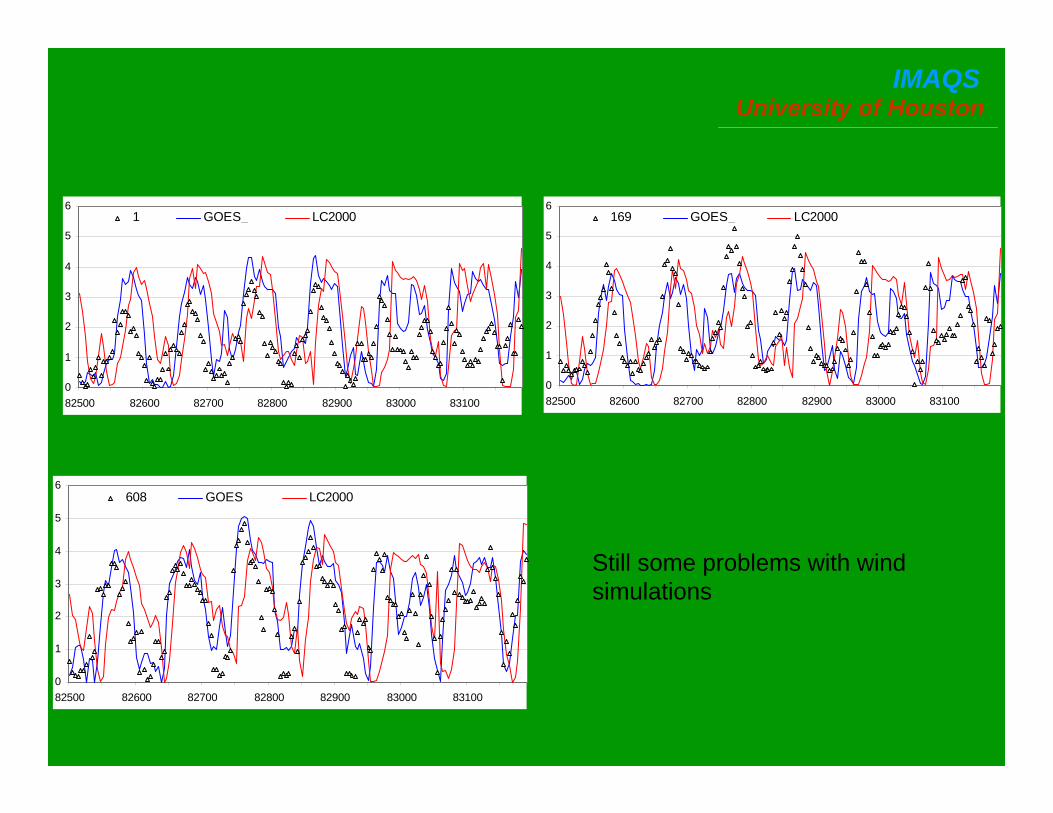
Still some problems with wind simulations
University of HoustonIMAQS
Air Quality Simulation
Biogenic Emissions Estimates
Data:
1. Use the same PASR as base case2. Use 2000 LU canopy temperature using MM5/NOAH3. Use 1990 LU canopy temperature using MM5/NOAH4. 2000 Leaf mass density data from Nowak
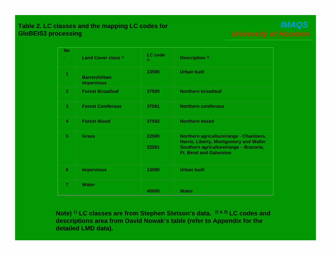
University of HoustonIMAQSTable 2. LC classes and the mapping LC codes for
GloBEIS3 processing
No. Land Cover class 1) LC code
2) Description 3)
1Barren/Urban impervious
13590 Urban built
2 Forest Broadleaf 37590 Northern broadleaf
3 Forest Coniferous 37591 Northern coniferous
4 Forest Mixed 37592 Northern mixed
5 Grass 22590
22591
Northern agriculture/range - Chambers, Harris, Liberty, Montgomery and WallerSouthern agriculture/range – Brazoria, Ft. Bend and Galveston
6 Impervious 13590 Urban built
7 Water40000 Water
Note) 1) LC classes are from Stephen Stetson’s data. 2) & 3) LC codes and descriptions area from David Nowak’s table (refer to Appendix for the detailed LMD data).
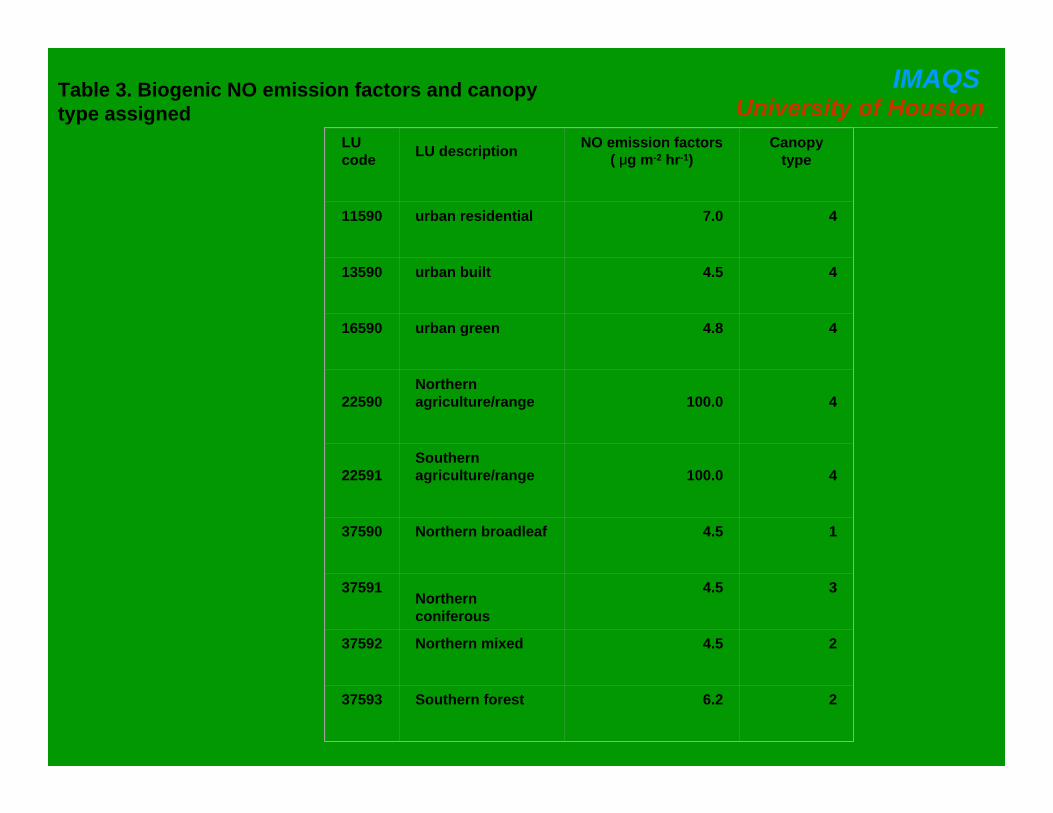
University of HoustonIMAQSTable 3. Biogenic NO emission factors and canopy
type assignedLU code LU description NO emission factors
( μg m-2 hr-1)Canopy
type
11590 urban residential 7.0 4
13590 urban built 4.5 4
16590 urban green 4.8 4
22590Northern agriculture/range 100.0 4
22591Southern agriculture/range 100.0 4
37590 Northern broadleaf 4.5 1
37591Northern coniferous
4.5 3
37592 Northern mixed 4.5 2
37593 Southern forest 6.2 2

University of HoustonIMAQS
LC shapedata
For HGA 8 Countiesfrom Stephen Stetson
MIMS
TCEQ LU data
Original 4-kmdomain
Gridding & post-processing
Replacing LU & LMD data for HGA
New LMDdata
For HGA 8 Countiesfrom David Nowak
New biogenic emission processing
GloBEIS3 Modifiedemissions
Temp &PAR data
From TCEQ
Additionalinput data
Modified estimation of GloBIES3 biogenic emissions utilizing new land use (LU), land cover (LC), and leaf mass density (LMD) data for the Houston-Galveston Airshed (HGA).

University of HoustonIMAQS
TCEQ Bio.LU/LC
TFS LANDSAT basedLand Cover
University of HoustonIMAQS
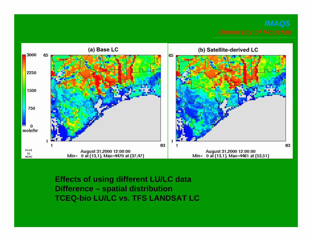
Effects of using different LU/LC dataDifference – spatial distributionTCEQ-bio LU/LC vs. TFS LANDSAT LC
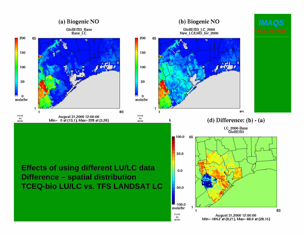
University of HoustonIMAQS
Effects of using different LU/LC dataDifference – spatial distributionTCEQ-bio LU/LC vs. TFS LANDSAT LC
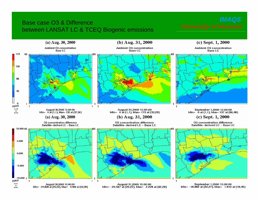
University of HoustonIMAQSBase case O3 & Difference
between LANSAT LC & TCEQ Biogenic emissions
University of HoustonIMAQS
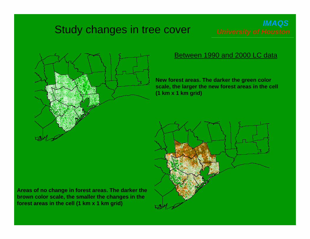
New forest areas. The darker the green color scale, the larger the new forest areas in the cell (1 km x 1 km grid)
Areas of no change in forest areas. The darker the brown color scale, the smaller the changes in the forest areas in the cell (1 km x 1 km grid)
Study changes in tree cover
Between 1990 and 2000 LC data
University of HoustonIMAQS
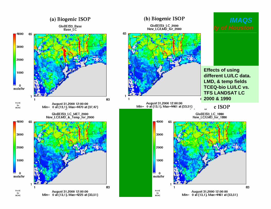
Effects of using different LU/LC data. LMD, & temp fieldsTCEQ-bio LU/LC vs. TFS LANDSAT LC 2000 & 1990

University of HoustonIMAQS
Biogenic emissions with Different met & lu/lc data
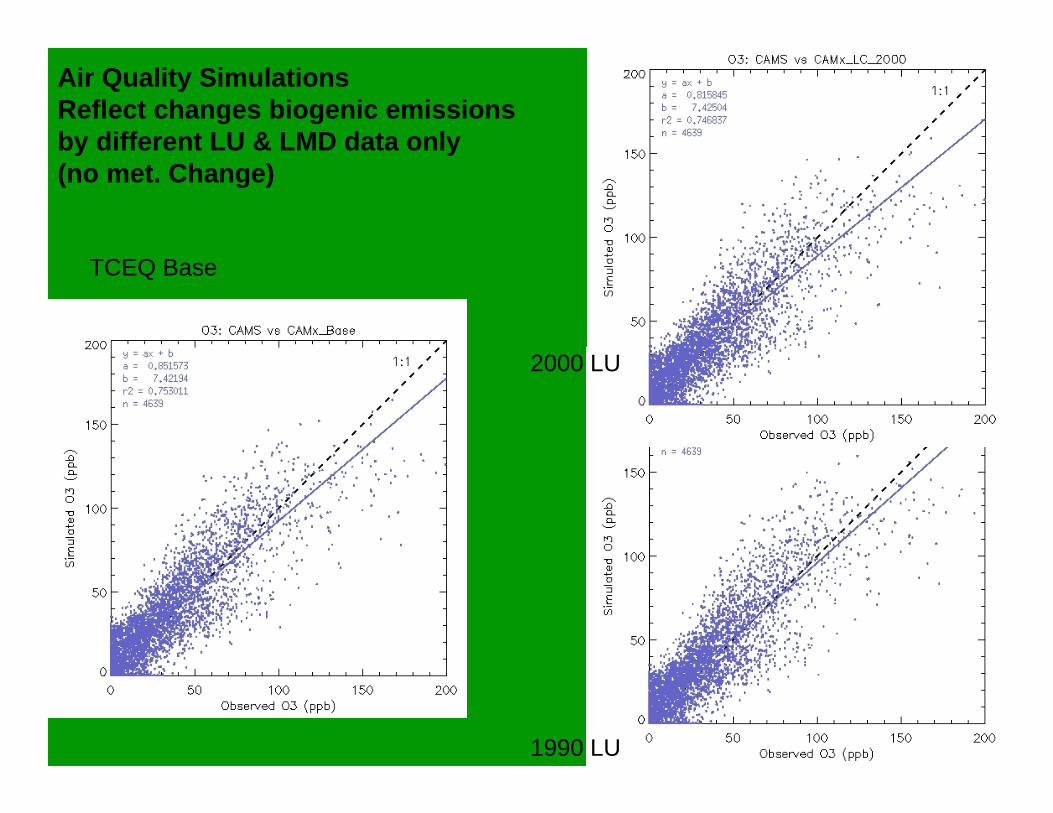
University of HoustonIMAQSAir Quality Simulations
Reflect changes biogenic emissions by different LU & LMD data only(no met. Change)
TCEQ Base
2000 LU
1990 LU
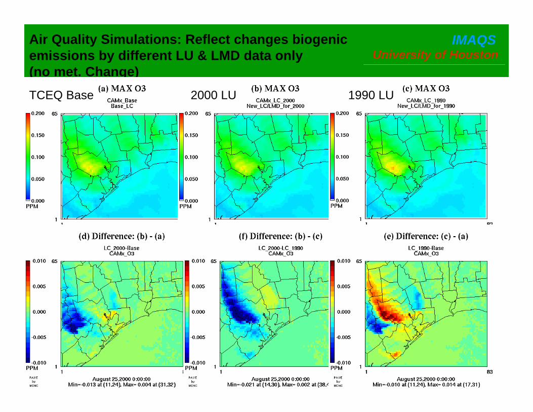
University of HoustonIMAQSAir Quality Simulations: Reflect changes biogenic
emissions by different LU & LMD data only(no met. Change)TCEQ Base 2000 LU 1990 LU

University of HoustonIMAQSAir Quality Simulations
Reflect changes biogenic emissions by different LU & LMD data & temp(no wind & PBL Change)
TCEQ Base
2000 LU
1990 LU
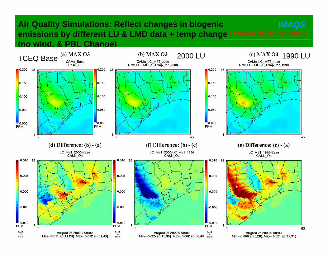
University of HoustonIMAQSAir Quality Simulations: Reflect changes in biogenic
emissions by different LU & LMD data + temp change(no wind. & PBL Change)TCEQ Base 2000 LU 1990 LU