Embed Size (px)
Citation preview

Effects of insecticides on freshwater invertebrate communities of small streams in
soy-production regions of South America
By
Elizabeth Shirin Hunt
A dissertation submitted in partial satisfaction of the
requirements for the degree of
Doctor of Philosophy
In
Environmental Science, Policy, and Management
in the
Graduate Division
of the
University of California, Berkeley
Committee in charge:
Professor Vincent H. Resh, Chair
Professor Stephanie M. Carlson
Professor G. Mathias Kondolf
Spring 2016

Effects of insecticides on freshwater invertebrate communities of small streams in
soy-production regions of South America
Copyright 2016
by
Elizabeth Shirin Hunt
1
Abstract
Effects of insecticides on freshwater invertebrate communities of small streams in
soy-production regions of South America
by
Elizabeth Shirin Hunt
Doctor of Philosophy in Environmental Science, Policy, and Management
University of California, Berkeley
Professor Vincent H. Resh, Chair
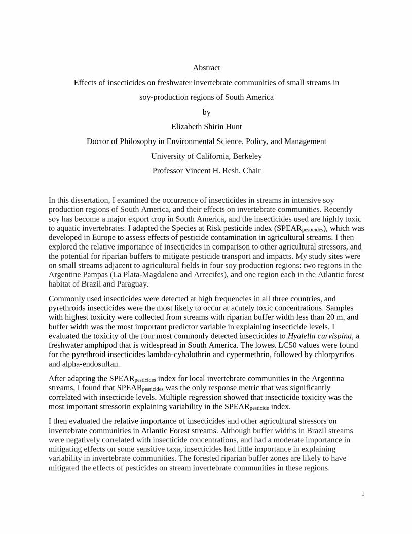
In this dissertation, I examined the occurrence of insecticides in streams in intensive soy
production regions of South America, and their effects on invertebrate communities. Recently
soy has become a major export crop in South America, and the insecticides used are highly toxic
to aquatic invertebrates. I adapted the Species at Risk pesticide index (SPEARpesticides), which was
developed in Europe to assess effects of pesticide contamination in agricultural streams. I then
explored the relative importance of insecticides in comparison to other agricultural stressors, and
the potential for riparian buffers to mitigate pesticide transport and impacts. My study sites were
on small streams adjacent to agricultural fields in four soy production regions: two regions in the
Argentine Pampas (La Plata-Magdalena and Arrecifes), and one region each in the Atlantic forest
habitat of Brazil and Paraguay.
Commonly used insecticides were detected at high frequencies in all three countries, and
pyrethroids insecticides were the most likely to occur at acutely toxic concentrations. Samples
with highest toxicity were collected from streams with riparian buffer width less than 20 m, and
buffer width was the most important predictor variable in explaining insecticide levels. I
evaluated the toxicity of the four most commonly detected insecticides to Hyalella curvispina, a
freshwater amphipod that is widespread in South America. The lowest LC50 values were found
for the pyrethroid insecticides lambda-cyhalothrin and cypermethrin, followed by chlorpyrifos
and alpha-endosulfan.
After adapting the SPEARpesticides index for local invertebrate communities in the Argentina
streams, I found that SPEARpesticides was the only response metric that was significantly
correlated with insecticide levels. Multiple regression showed that insecticide toxicity was the
most important stressorin explaining variability in the SPEARpesticide index.
I then evaluated the relative importance of insecticides and other agricultural stressors on
invertebrate communities in Atlantic Forest streams. Although buffer widths in Brazil streams
were negatively correlated with insecticide concentrations, and had a moderate importance in
mitigating effects on some sensitive taxa, insecticides had little importance in explaining
variability in invertebrate communities. The forested riparian buffer zones are likely to have
mitigated the effects of pesticides on stream invertebrate communities in these regions.
i
TABLE OF CONTENTS
Table of Contents .................................................................................................................... i
Dedication .............................................................................................................................. ii
Acknowledgments................................................................................................................. iii
CHAPTER 1: Introduction .................................................................................................... 1
CHAPTER 2: Insecticide concentrations in stream sediments of soy production
regions of South America ...................................................................................................... 7
CHAPTER 3: Acute toxicity of four insecticides to the South American
amphipod Hyalella curvispina based on sediment and water exposures ............................. 39
CHAPTER 4: Effects of insecticides on stream invertebrate communities
in soy production regions of the Argentine Pampas ............................................................ 61
CHAPTER 5: Relative importance of agricultural stressors affecting
invertebrate communities in Atlantic Forest streams, and the effectiveness
of forested riparian buffers in mitigating them .................................................................... 90
CHAPTER 6: Conclusions and future directions .............................................................. 122

ii
DEDICATION
Dedicated to Oof and the Ancient One, and to all living beings on this extraordinary planet
(especially the weird ones)

iii
ACKNOWLEDGEMENTS
Words cannot adequately express my gratitude to the many people who have supported me,
advised me, and assisted me throughout this grand adventure. First, I want to give thanks to my
advisor, Vince Resh, who taught me to ask for forgiveness rather than permission, and to always
prioritize my health and happiness and the important people in my life instead of work. He shares
my love for travel and never ceases to amaze me with his ability to review my drafts, provide
advice, and compose letters of recommendation almost instantaneously from far off places. I
could not have asked for a more supportive mentor, and I can only strive to come close to being
as giving a person as he is.
I am indebted to Matt Kondolf for his continued support and advice (starting when I took his
river restoration class long before my doctoral work), for serving on both my qualifying
committee and my dissertation committee, and for generously loaning me his canine companion
Yaku in moments of need. I also thank Stephanie Carlson for serving on both my qualifying
committee and my dissertation committee, and for helping me form a solid foundation in aquatic
ecology while preparing for my research. I thank Adina Merenlender for serving on my
qualifying committee, for forcing me to understand the necessary statistics, and for making me
squirm during my qualifying exam. I am grateful to Donald Weston for serving on my qualifying
committee and also for helping me prepare to conduct bioassays in Argentina and answering my
many pesky questions.
So many members of the Resh lab have provided me with advice, guidance and friendship during
the last six years. Kevin Lunde, Justin Lawrence, Kaua Fraiola, and Joanie Damerow initiated me
to the wonderful world of grad school and ESPM, and helped me learn all about aquatic
invertebrates and various other fascinating things. Mike Peterson and Natalie Stauffer provided
encouragement during the dark days of dissertation writing, and Jacky Chiu provided hours of
stimulating conversation about statistics, my favorite topic. Patina Mendez gave me all kinds of
advice about all kinds of things.
I am also deeply indebted to my adoptive lab in Argentina, the Bonetto lab at ILPLA. To Carlos
Bonetto for reluctantly agreeing to support (almost) all of my crazy ideas, despite my tendency to
“meterme en líos”, and to Natalia Marrochi and Any Scalise for accompanying me on my
adventures and bailing me out of trouble. To Silvia Fanelli for helping me with the chemistry and
for correcting my many mistakes, and to Hernan Mugni and Marina Solis for helping me get
started with field work.
I am especially grateful to several collaborators without whom I could not have accomplished my
research. Michael Lydy at the University of Southern Illinois provided invaluable assistance with
the pesticide analysis part of my work, and worked with me over the years to adapt the methods.
John Kochalka of the Museo de Historia Nacional de Paraguay helped me obtain collection
permits, organize logistics, and find field assistants, and spent countless hours over the
microscopes with me. Daniel Buss of FIOCRUZ Brazil organized the field logistics and helped
me with the study design in Brazil, introduced me to many valuable contacts, and provided
advice on data analysis and interpretation. Michelli Ferronato allowed us to use the excellent
laboratory facilities of the Pontifícia Universidade Católica do Paraná in Brazil, coordinated field
logistics and student assistants, and provided guidance on invertebrate identifications. Matthias
Liess of the University of Helmholz in Germany helped me modify the Species at Risk index for
South America, and provided advice on multiple issues through the years.
iv
Several individuals generously contributed their time and expertise to assist me. Bill Shepard
interrupted his “retired” life to help me learn all about the Elmidae beetles of Paraguay, and Jim
Carter of USGS helped me calculate various bioassessment metrics. Carolina Vieira da Silva
spent six months working in our lab through the CAPES international exchange program of
Brazil, and helped me learn how to identify the heads of oligochaete worms, including the little
smiles on their faces .
We had many field assistants who worked long hours sampling streams in both scorching heat
and torrential downpours, and then spent even longer days sorting invertebrate samples: Carlos
Aguilar, Gustavo Godoy, Augusto Maidana, Sol Hernandez, Cecilia, Guido, Gabriela Romero,
Liza Logray, and Samaila Pujarra, and Anni Ala. I greatly appreciate their enthusiasm and
dedication – and they made the project so much more fun!
In addition to my official collaborators, there were many other organizations that provided
invaluable help with field logistics, including Pro Cosara, Museo Nacional de Historia Natural
Paraguay, Guyra Paraguay, World Wildlife Fund Paraguay, Vida Silvestre Argentina, Pontifícia
Universidade Católica do Paraná, and Instituto Ambiental do Paraná, Brazil.
My research was supported by grants from the Agencia Nacional de Promoción Científica y
Tecnológica (Argentina – PICT 2010-0446) and the Conselho Nacional de Desenvolvimento
Científico e Tecnológico/Programa de Excelência em Pesquisa (Brazil – Grant No. 400107/2011-
2). I was very lucky to receive fellowships from the National Science Foundation and the
Fulbright Commission, as well as the University of California Dissertation Year fellowship.

1
CHAPTER 1
Introduction
2
Introduction
In recent years, soybean production has become a major export crop for multiple countries in
South America, including Brazil, Argentina, Paraguay, Uruguay, and Bolivia. Between 1986 and
2010, the total area in soy production in the Americas increased from 37 to 79 million hectares
(Mha), and most of this expansion occurred in Argentina, Brazil, and Paraguay (Garrett et al.
2013). Between 1995 and 2011, soy cultivation area expanded by 126% and 209% in Brazil and
Argentina, respectively (Castanheira and Freire 2013). In Paraguay, soy cultivation area
increased from 1.3 Mha in 2000-2001 to 2 Mha in 2007-2008 (Garcia-Lopez and Arizpe 2010).
Land use changes caused by expansion of soy cultivation in South America have raised a number
of environmental concerns, including reductions in ecosystem complexity, loss of biodiversity,
deforestation, increased erosion, adverse effects of agrochemicals, and increased greenhouse gas
emissions (Botta et al. 2011; Castanheira and Freire 2013; Lathuilliere et al. 2014).
Conversion of land to intensive agriculture can result in degradation of adjacent streams and
stream ecosystem through impacts such as nutrient enrichment, sedimentation, pesticides,
deforestation (Gücker et al., 2009; Jones et al., 2001; Matthaei et al., 2010). Benthic
macroinvertebrate communities have been shown to be adversely impacted by agriculture
adjacent to streams through multiple mechanisms. Agriculture-related stressors can include
habitat degradation (e.g. loss of cover, deposition of fine sediments), hydrological modification
(e.g. channelization, less diversity in pool/run/riffle regimes) and impacts to water quality (e.g.
pesticide toxicity, nutrient eutrophication, increased turbidity and conductivity)(Matthaei et al.,
2010; Stehle and Schulz, 2015; Stone et al., 2005; Whiles et al., 2000).
Pesticides used in agriculture can have severe impacts on stream water quality and ecosystems.
A recent metaanalysis of 838 studies across 73 countries found that over 50% of measured
insecticide concentrations in water bodies exceeded regulatory threshold levels for surface
waters or sediments (Stehle and Schulz, 2015). Arecent analysis of data from Europe and
Australia reported that pesticides reduced both species and family richness of aquatic
invertebrate communities (Beketov et al., 2013). The insecticides used in soy production in
South America are known to be especially toxic to aquatic invertebrates (Mugni et al., 2011).
A life cycle analysis of the soy-biodiesel crops produced in Argentina for export concluded that
the aquatic toxicity impacts from soy-production pesticides were substantially higher than their
terrestrial toxicity impacts, with the pyrethroid insecticide cypermethrin being the main
contributor (Panichelli et al. 2009). Although application rates of the herbicide glyphosate in the
cultivation of genetically modified soy are much higher than those of fungicides and insecticides,
the potential toxic impact of glyphosate and other herbicides in aquatic areas near soy production
systems of South America are considered to be negligible compared to those of fungicides and
insecticides (Nordborg et al. 2014). Insecticide application rates are approximately double those
of fungicides, and the insecticides most frequently used in soy production have very high aquatic
toxicity (Nordborg et al. 2014).
Stream buffer width may be one of the most important factors in mitigating transport of
pesticides, sediment,and other pollutants to streams in agricultural areas (Bunzel et al., 2014;
Jones et al., 2001; Rasmussen et al., 2011; Stone et al., 2005), butbuffer zone requirements differ
substantially among the three major soy production countries in South America. Riparian buffer
zones are required to be maintained in both Brazil and Paraguay, although specific requirements
are in flux. For example, Paraguay, requires a protected zone of 100 m around all water bodies.

3
In Brazil, a new forest code was approved in 2012 (Law No.12.651/12) establishing that riparian
buffer zone requirements should vary with the general use of the land adjacent to the water body,
the aquatic environment, the stream width, and the size of the rural property. In contrast, in
Argentina there are no national requirements for stream buffers.
In this dissertation, I examined the occurrence of insecticides in small streams in intensive soy
production regions of South America, and their effects on stream invertebrate communities. I
adapted the Species at Risk (SPEAR) pesticide bioassessment index (SPEARpesticides), which was
developed in Europe to assess effects of pesticide contamination in agricultural streams (Liess
and Von der Ohe, 2005), for my study region. In addition, I explored the relative importance of
insecticide toxicity effects in comparison to other agricultural stressors on invertebrates, and the
potential for riparian buffers to mitigate pesticide transport and other adverse effects on stream.
Study regions
The study sites were located on small streams that flowed through agricultural fields in four soy
production regions: two regions in the Argentina Pampas (La Plata-Magdalena and Arrecifes),
and one region each in the former Atlantic forest habitat of Brazil and Paraguay (Figure 1). In the
La Plata-Magdalena region, the principal land use was cattle grazing, with scattered plots of soy
production and other agriculture. In the three other regions, intensive soy production was the
predominant land use. In the La Plata-Magdalena region, five streams were sampled during five
monitoring events in the 2011 to 2012 season only, including three sampling sites in one
watershed and the remaining sites in separate watersheds. In the Arrecifes region, 16 sites were
sampled over three years (2012-2014), and all sampling sites were on tributaries of the Arrecifes
River. In Paraguay, 17 sites were sampled over two seasons (January and December 2013), and
all sampling sites were on tributaries of the Pirapó River in the state of Itapúa. In Brazil, 18 sites
were sampled once in November 2013, and all sampling sites were on tributaries of the San
Francisco River in the state of Paraná. All study watersheds were tributaries of the Paraná/La
Plata River.
Chapter Overview
In Chapter 2, I describe the results of my investigations on concentrations and detection
frequencies of insecticides in the four study regions. I also conducted a regression analysis to
evaluate the influence of riparian buffer width on insecticide concentrations in streams.
In Chapter 3, I evaluated the toxicity of the four most commonly detected insecticides
(cypermethrin, lambda-cyhalothrin, chlorpyrifos and endosulfan) to Hyalella curvispina, a
freshwater amphipod that is widespread in South America and is closely related to H. azteca, a
standard test species in the United States. For each of these insecticides in both sediment and
water, I determined median lethal concentration (LC50) values for H. curvispina. I then
calculated species sensitivity distributions (SSDs) for freshwater invertebrate taxa using results
of my study and other available data.
In Chapter 4, I investigated relationships among insecticide concentrations and aquatic
invertebrate communities in 22 streams of two soy production regions of the Argentine Pampas
4
over three growing seasons. Along with standard macroinvertebrate bioassessment metrics, I
applied the SPEARpesticides index to evaluate relationships between sediment insecticide toxic
units (TUs) and invertebrate communities associated with both benthic habitats and emergent
vegetation. I then performed a multiple regression analysis to evaluate the influence of multiple
agricultural stressors and habitat variables.
In Chapter 5, I evaluatedthe influence and relative importance of insecticides and other
agricultural stressors in determining variability in invertebrate communities in small streams in
intensive soy production regions of Brazil and Paraguay. The riparian buffer zones in these
regions generally contained native Atlantic forest remnants and/or introduced tree species at
various stages of growth, and I evaluated the effectiveness of the riparian buffer in mitigating
adverse effects of soy production on streams.
In Chapter 6, I summarize the overall conclusions and important findings of my dissertation
research. I also lay outsome possible explanations for why the findings for insecticide effects on
invertebrate communities differed between the Argentina Pampas streams and the Atlantic Forest
streams. I then discuss future research and management needs in the region.
References
Beketov, M.A., Kefford, B.J., Schafer, R.B., Liess, M., 2013. Pesticides reduce regional
biodiversity of stream invertebrates. Proc. Natl. Acad. Sci. 110, 11039–11043.
doi:10.1073/pnas.1305618110
Bunzel, K., Liess, M., Kattwinkel, M., 2014. Landscape parameters driving aquatic pesticide
exposure and effects. Environ. Pollut. 186, 90–97. doi:10.1016/j.envpol.2013.11.021
Gücker, B., BoëChat, I.G., Giani, A., 2009. Impacts of agricultural land use on ecosystem
structure and whole-stream metabolism of tropical Cerrado streams. Freshw. Biol. 54, 2069–
2085. doi:10.1111/j.1365-2427.2008.02069.x
Jones, K.B., Neale, A.C., Nash, M.S., Van Remortel, R.D., Wickham, J.D., Riitters, K.H.,
O’neill, R.V., 2001. Predicting nutrient and sediment loadings to streams from landscape
metrics: a multiple watershed study from the United States Mid-Atlantic Region. Landsc. Ecol.
16, 301–312.
Liess, M., Von der Ohe, P.C.D., 2005. Analyzing effects of pesticides on invertebrate
communities in streams. Environ. Toxicol. Chem. 24, 954–965.
Matthaei, C.D., Piggott, J.J., Townsend, C.R., 2010. Multiple stressors in agricultural streams:
interactions among sediment addition, nutrient enrichment and water abstraction: Sediment,
nutrients & water abstraction. J. Appl. Ecol. 47, 639–649. doi:10.1111/j.1365-
2664.2010.01809.x
Mugni, H., Ronco, A., Bonetto, C., 2011. Insecticide toxicity to Hyalella curvispina in runoff and
stream water within a soybean farm (Buenos Aires, Argentina). Ecotoxicol. Environ. Saf. 74,
350–354. doi:10.1016/j.ecoenv.2010.07.030
Rasmussen, J.J., Baattrup-Pedersen, A., Wiberg-Larsen, P., McKnight, U.S., Kronvang, B.,
2011. Buffer strip width and agricultural pesticide contamination in Danish lowland streams:

5
Implications for stream and riparian management. Ecol. Eng. 37, 1990–1997.
doi:10.1016/j.ecoleng.2011.08.016
Stehle, S., Schulz, R., 2015. Agricultural insecticides threaten surface waters at the global scale.
Proc. Natl. Acad. Sci. 112, 5750–5755. doi:10.1073/pnas.1500232112
Stone, M.L., Whiles, M.R., Webber, J.A., Williard, K.W.J., Reeve, J.D., 2005.
Macroinvertebrate Communities in Agriculturally Impacted Southern Illinois Streams. J.
Environ. Qual. 34, 907. doi:10.2134/jeq2004.0305
Whiles, M.R., Brock, B.L., Franzen, A.C., Dinsmore, II, S.C., 2000. Stream Invertebrate
Communities, Water Quality, and Land-Use Patterns in an Agricultural Drainage Basin of
Northeastern Nebraska, USA. Environ. Manage. 26, 563–576. doi:10.1007/s002670010113
6
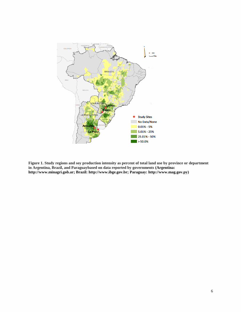
Figure 1. Study regions and soy production intensity as percent of total land use by province or department
in Argentina, Brazil, and Paraguaybased on data reported by governments (Argentina:
http://www.minagri.gob.ar; Brazil: http://www.ibge.gov.br; Paraguay: http://www.mag.gov.py)

7
CHAPTER 2
Insecticide concentrations in stream sediments of
soy production regions of South America

8
Insecticide concentrations in stream sediments of soy production regions of South America
Abstract
Concentrations of 17 insecticides were measured in sediments collected from 53 streams in soy
production regions of South America (Argentina in 2011-2014, Paraguay and Brazil in 2013)
during peak application periods. Although environmental regulations are quite different in each
country, commonly used insecticides were detected at high frequencies in all regions. Maximum
concentrations (and detection frequencies) for each sampling event ranged from: 1.2–7.4 ng/g dw
chlorpyrifos (56-100%); 0.9–8.3 ng/g dw cypermethrin (20-100%); 0.42–16.6 ng/g dw lambda-
cyhalothrin (60-100%); and 0.49–2.1 ng/g dw endosulfan (13-100%). Other pyrethroids were
detected less frequently. Banned organochlorines were most frequently detected in Brazil. In all
countries, cypermethrin and/or lambda-cyhalothrin toxic units (TUs), based on Hyalella azteca
LC50 bioassays,were occasionally >0.5 (indicating likely acute toxicity), while TUs for other
insecticides were <0.5. All samples with total insecticide TU> 1 were collected from streams
with riparian buffer width<20m. A multiple regression analysis that included five landscape and
habitat predictor variables for the Brazilian streams examined indicated that buffer width was the
most important predictor variable in explaining total insecticide TU values. While Brazil and
Paraguay require forested stream buffers, there were no such regulations in the Argentine
Pampas, where buffer widths were smaller. Multiple insecticides were found in almost all stream
sediment samples in intensive soy production regions, with pyrethroids most often occurring at
acutely toxic concentrations, and the greatest potential for insecticide toxicity occurring in
streams with minimum buffer width < 20m.
Introduction
In recent years, soybean production has become a major export crop for multiple countries in
South America, including Brazil, Argentina, Paraguay, Uruguay, and Bolivia. Between 1986 and
2010, the total area in soy production in the Americas increased from 37 to 79 million hectares
(Mha), and most of this expansion occurred in Argentina, Brazil, and Paraguay (Garrett et al.
2013). Between 1995 and 2011, soy cultivation area expanded by 126% and 209% in Brazil and
Argentina, respectively (Castanheira and Freire 2013). In Paraguay, soy cultivation area
increased from 1.3 Mha in 2000-2001 to 2 Mha in 2007-2008 (Garcia-Lopez and Arizpe 2010).
Land use changes caused by expansion of soy cultivation in South America have raised a number
of environmental concerns, including reductions in ecosystem complexity, loss of biodiversity,
deforestation, increased erosion, adverse effects of agrochemicals, and increased greenhouse gas
emissions (Botta et al. 2011; Castanheira and Freire 2013; Lathuilliere et al. 2014).
A life cycle analysis of the soy-biodiesel crops produced in Argentina for export concluded that
the aquatic toxicity impacts from soy-production pesticides were substantially higher than their
terrestrial toxicity impacts, with the pyrethroid insecticide cypermethrin being the main
contributor (Panichelli et al. 2009). Although application rates of the herbicide glyphosate in the
cultivation of genetically modified soy are much higher than those of fungicides and insecticides,
the potential toxic impact of glyphosate and other herbicides in aquatic areas near soy production
systems of South America are considered to be negligible compared to those of fungicides and
insecticides (Nordborg et al. 2014). Insecticide application rates are approximately double those

9
of fungicides, and the insecticides most frequently used in soy production have very high aquatic
toxicity (Nordborg et al. 2014).
Insecticides are typically applied several times to each soy crop, and are used primarily to control
lepidopteran pests during plant growth, and hemipteran pests during the fruiting stage.
Lepidopteran pests are often controlled by applications of chlorpyrifos, an organophosphate, and
hemipteran pests by endosulfan, an organochlorine. Pyrethroids, especially cypermethrin, are
commonly used for both types of pests, and are often applied at the same time as other pesticides
(Di Marzio et al. 2010; OPDS 2013). In Brazil, diamides and growth inhibitors are becoming
more frequently used to control lepidopteran pests, while mixtures of neonicotinoid and
pyrethroid insecticides are often used to control hemipteran pests. Contrary to recommendations
from pest control advisors, pesticide applications for soy production in Brazil are primarily done
prophylactically, with four to six applications per year (Bueno et al. 2011). The same trend is
true in Argentina, with cypermethrin often being added to herbicide applications in order to
prevent lepidopteran pests from laying eggs (OPDS 2013). Moreover, the systemic neonicotinoid
insecticide imidacloprid is commonly used in Paraguay and Brazil as a seed treatment, and is
also applied as a spray later in the season along with pyrethroids, such as lambda-cyhalothrin or
cypermethrin.
Multiple studies have detected soy production insecticides in both sediment and water collected
from streams in Argentina and Brazil; however, most studies did not include all of the most
frequently used insecticides, and data were not always comparable because of the use of variable
matrices, methods, and reporting limits (Jergentz et al. 2004a; Mugni et al. 2010; Di Marzio et al.
2010; Marino and Ronco 2005; Possavatz et al. 2014; Casara et al. 2012; Miranda et al. 2008;
Laabs et al. 2002). Several studies in Argentina and Brazil have found associations between
stream insecticide concentrations and effects to aquatic invertebrates and/or fish (Jergentz et al.
2004a; Rico et al. 2010; Di Marzio et al. 2010; Mugni et al. 2010; Chelinho et al 2012); however,
no studies of this type have been published on data collected from Paraguay.
Stream buffer width may be one of the most important factors in mitigating transport of
pesticides to streams in agricultural areas (Bunzel et al. 2014; Rasmussen et al. 2011), but buffer
zone requirements differ substantially among the three countries included in the present study.
Riparian buffer zones are required to be maintained in both Brazil and Paraguay, although
specific requirements are in flux. For example, in Paraguay, Resolution 485/03 by the Ministry
of Agriculture requires a protected zone of 100 m around all water bodies. In Brazil, a new forest
code was approved in 2012 (Law No.12.651/12) establishing that riparian buffer zone
requirements should vary with the general use of the land adjacent to the water body, the aquatic
environment, the stream width, and the size of the rural property. As a general rule for stream
widths of 10m or less, the legislation requires a buffer width of 15m of native riparian forest in
rural areas or 30m if in areas newly converted for rural activities. In contrast, in Argentina there
are no national requirements for stream buffers. Moreover, stream buffer zones in the Argentine
Pampas are generally unregulated, and many small streams in the most intensive soy production
regions of the Santa Fe and Cordoba provinces are completely channelized with crops planted
right up to the banks (no buffer zones). Some Argentine provinces do prohibit pesticide
application within a specific distance from surface water (Chaco: Law 7032 – DR 1567/13;
Formosa: Law 1163 – DR 109/02; Río Negro: Law 2175 – DR 769/94).
10
The objectives of the present study were to: (1) measure and compare insecticide concentrations
in sediments collected from streams in four soy production regions: two in the Pampas of
Argentina, one in eastern Paraguay, and one in south Brazil; (2) evaluate the potential for acute
toxicity of insecticides on sensitive aquatic invertebrate taxa, such as Hyalella spp.; and, (3)
evaluate the relationship between buffer strip widths and insecticide concentrations in stream
sediments, taking into account the influence of other environmental variables.
Methods
Study Locations and Sampling Schedule
The study sites included small streams that flowed through agricultural fields in four soy
production regions: two regions in the Argentina Pampas (La Plata-Magdalena and Arrecifes),
and one region each in the former Atlantic forest habitat of Brazil and Paraguay (Figure 1). In the
La Plata-Magdalena region, the principal land use was cattle grazing, with scattered plots of soy
production and other agriculture. In the three other regions, intensive soy production was the
predominant land use. In the La Plata-Magdalena region, five streams were sampled during five
monitoring events in the 2011 to 2012 season only, including three sampling sites in one
watershed and the remaining sites were located in separate watersheds. In the Arrecifes region,
16 sites were sampled over three years (2012-2014), and all sampling sites were on tributaries of
the Arrecifes River. In Paraguay, 17 sites were sampled over two seasons (January and
December 2013), and all sampling sites were on tributaries of the Pirapó River in the state of
Itapúa. In Brazil, 18 sites were sampled once in November 2013, and all sampling sites were on
tributaries of the San Francisco River in the state of Paraná. All study watersheds were tributaries
of the Paraná/La Plata River.
Streams selected for the present study were not channelized, and most had a buffer strip of at
least 5 m from the crops (Tables S1, S2). In the Brazil and Paraguay streams, the buffer zones
generally contained Atlantic forest remnants and/or introduced tree species. In both Argentina
regions, the buffers generally contained grasses and low shrubs with occasional trees. Minimum
buffer widths were measured immediately upstream of sampling sites, and confirmed with
LANDSAT images in Brazil and Paraguay. However, confirmation with LANDSAT images was
not possible in Argentina, because there generally were not forested areas around streams and it
was difficult to differentiate herbaceous vegetation from cropland. Catchments were delineated
using topographical maps to estimate catchment size, and in Brazil and Paraguay the percent
forest and percent agriculture within each catchment were estimated using LANDSAT images.
Substrates in streams of both Argentina regions generally consisted of sediment with no rocks
and little woody debris, although a few sites in Arrecifes contained some gravel. Substrates in
Brazil and Paraguay streams usually contained relatively large amounts of rocks and/or cobble,
and tended to have higher gradients and faster velocities than streams in Argentina. Stream
depths ranged from about 0.6 m to > 2 m (although all except two in the La Plata region were < 1
m), and widths ranged from about 3 m to about 25 m (Table S2). While streams in Brazil and
Paraguay were generally free of aquatic vegetation, most streams in Argentina included
emergent vegetation (e.g.Typha spp. and Scirpus spp.) and submerged vegetation (e.g.
Potamogeton, Ceratophyllum and Egeria), and many in the La Plata-Magdalena region were also
characterized by abundant floating vegetation (e.g.Eichornia, Lemna and Azolla).
11
Stream sampling was timed to coincide with peak insecticide application periods, which varied
by region depending on planting time. Soy can either be planted as an early season crop or a late
season crop. In the Argentine Pampas, the early season crop was planted in October or
November and harvested in February, while in Paraguay and southern Brazil it was planted in
September or October and harvested in January. The late season crop was typically planted
between December and February and harvested several months later. In the Argentine Pampas,
peak insecticide applications for soy production usually occurred in late December to early
February, while in Paraguay and southern Brazil they occurred in November and December.
Field water quality measurements
At each sampling site, pH, conductivity, dissolved oxygen, and temperature were measured with
a Yellow Springs Instruments SI 556 multi-parameter probe (Yellow Springs, OH, USA).
Turbidity was measured with a portable turbidity meter (Hanna Instruments 93414, Woonsocket,
RI, USA), and maximum and average water velocities were measured with a current meter
(Global Water FP311, College Station, TX, USA).
Sample collection
Based on the properties of the insecticides analyzed, streambed sediments rather than water
samples were examined. Most insecticides commonly used in soy production in South America
have low water solubility, and a high affinity to bind to soil and sediments based on chemical
properties, such as koc (Tables 1 and 2). Moreover, pesticide concentrations in stream water often
occur as ephemeral events, and peak immediately following the first rain after application
(Schäfer et al. 2011). However, elevated concentrations of the target insecticides can persist
longer when they are associated with sediments (Jergentz et al. 2005). In all of the regions
studied, precipitation occurs often during the peak pesticide application period. Sampling events
in the present study were generally timed to occur within a week after a heavy rainfall during the
peak insecticide application season.
Sediment samples were collected with a stainless steel scoop from the top two centimeters,
generally from depositional areas depending on depth, access, and availability of sediment.
Composite samples were prepared from 3 to 5 locations at each site and placed in pesticide-free
amber glass jars with Teflon lids, which were kept in coolers on ice until arrival at the laboratory
where they were kept refrigerated until extraction (maximum of 5 d), or frozen for later
extraction (maximum of 4 mo). After thoroughly homogenizing each sample in the laboratory,
an aliquot was taken from each sample for analysis of total organic carbon by ferrous sulfate
titration (USDA 1996). A separate sample was collected at each location for sediment grain size
analysis (Table S2).
Chemicals
All pesticide standards, internal standards (lindane d6 and chlorpyrifos d10), and the surrogate
standard decachlorobiphenyl (DCBP) were purchased from Accustandard and had purities >
93% as reported by Accustandard (New Haven, CT, USA). The solvents used in extractions and

12
analysis were all pesticide grade. Granular copper used in sample extractions was purified by
covering with methylene chloride, shaken vigorously, and allowed to dry in the hood for 24 h.
During the first 18 months of the project, gas chromatography coupled with electron capture
detection (GC-ECD) was used to analyze the insecticides reported to be most frequently used in
Argentina on soy crops including cypermethrin, chlorpyrifos, lambda-cyhalothrin, and
endosulfan (Table 1).
Throughout the project, information on pesticide use was obtained by interviewing personnel
from government agencies, universities, pesticide manufacturers, and grower cooperatives in all
three countries studied, and by searching documents from all sources including grey literature. In
2013 and 2014, analysis of organochlorine pesticides was added, because of concerns about their
potential illegal application (Table 2). For quantification of the larger analyte list, the more
advanced method of a GC coupled with a mass spectrometer (GC-MS) was used. Analysis of
additional pyrethroids and the synergist piperonyl butoxide (PBO) was also added when the new
method was implemented (Table 2). Although PBO is not present in insecticide formulations
sold for use in soy production, it is possible that growers are mixing it with pyrethroid pesticides
to increase their efficacy, or it may come from other sources such as tick control in farm animal
production.
Extraction procedure
Extraction procedures followed You et al. (2004b), who demonstrated that sonication provided
good recovery for the pesticides of interest (You et al. 2004b; You and Lydy 2007; You et al.
2008). After each sample was thoroughly homogenized manually, approximately 20 g of
sediment (wet weight) was removed, spiked with 100 ng of thesurrogate DCBP, and mixed with
4 g of copper and anhydrous Na2SO4 in an ice-cooled beaker until the sediment was sufficiently
dry. A 50-ml aliquot of a 50:50 mixture of acetone and methylenechloride was added, and the
mixture was sonicated for 5 minutes in 3-s pulse mode using a high-intensity ultrasonic
processor at an amplitude of 60 (model VCX 500; Sonics and Materials, Newtown, CT, USA).
The extract was decanted and filtered through a Whatman no. 41 filter paper (Whatman,
Maidstone, UK) filled with approximately 2 g of anhydrous Na2SO4. This procedure was
repeated two additional times with a sonication time of 5 minutes each time. Extracts were
combined and decreased to approximately 1- 2 ml by evaporation.
Cleanup of extracts
Prior to cleanup, extracts for the methylene chloride andacetone:methylene chloride mixture
were solvent-exchanged to hexane, and the volumes of all treatments were reduced to 0.5 to 1ml
under nitrogen gas. A Envi-Carb II/primary - secondary amine solid phase extraction (SPE)
cartridge was connected to a vacuum manifold, adding 1 g of purified sodium sulfate to the top
of the sorbent to remove any residual water, then primed with 3 ml of hexane.The extract was
then loaded onto the cartridge. Next, 7 ml of a 30:70 methylene chloride/hexane mixture was
added to the cartridge, the extract was removed from the vacuum manifold and reduced to a
volume of 0.5 to 1 ml under nitrogen gas. The collection vial was then rinsed three times with
0.5 ml of a 0.1% acetic acid in hexane solution and added to the GC vial. The volume was
13
further reduced to 1 ml for analysis. The acidification step was used to minimize isomerization of
the pyrethroids (You and Lydy 2007). Granular copper was added to extracts and placed on a
shaker (Lab Rotator model G-2, New Brunswick Scientific Co., NJ, USA) for 2 to 3 h when high
residual sulfur was detected in the extracts. Once at final volume, internal standards were added
at a concentration of 20 ng/ml (for GC/MS analysis only) and the samples were stored at -20°C
until analysis.
Analytical methods
Gas Chromatograph-Electron Capture Detector
During the 2011 to early 2013 sampling period, analysis of the most commonly used insecticides
(Table 1) was performed on an Agilent 6890 series GC equipped with an Agilent7683
autosampler and a micro- ECD (Agilent Technologies, Palo Alto, CA, USA). Two columns - a
HP-5MS (30 m x0.25 mm x0.25 µm film thickness; Agilent) and a DB-608 (30 m x0.25 mm
x0.25 µm film thickness; Agilent) were used to confirm the analytical results. Helium and
nitrogen were used as the carrier and makeup gas, respectively. A 2 µl sample was injected into
the GC using a pulsed split-less mode. For the DB-608, the oven was set at 100°C, heated first to
250°C at 10°C/min increments, then to 280°C at 3°C/min increments and finally held at 280°C
for 23 minutes. For the HP-5, the oven was set at 100°C, heated to 190°C at 5°C/min increments,
then to 214°C at 6°C/min increments, then to 280°C at 6°C/min increments and finally held at
280°C for 20 minutes. The flow rates of carrier gas were 1.7 ml/min and 2.0 ml/min for the HP-
5MS and DB-608 columns, respectively. Calibration was based on area using three to six
external standards. The standard solutions were made by dissolving 2.5,10, 50, 100, or 250 µg/L
of each pesticide and surrogate in hexane. The calibration curves generated were linear within
this concentration range. Qualitative identity was established using a retention window of 1%
with confirmation on a second column, and quantitation was performed using external standard
calibration.
Gas chromatography - mass spectrometry
For the 2013 to 2014 sampling period, a longer analyte list was used, and quantification of the
samples was completed on an Agilent 6850 gas chromatograph with a 5975 XL mass
spectrometer (Agilent Technologies, Palo Alto, CA, USA). Piperonyl butoxide was quantified in
electron impact (EI) mode, while all of the other target pesticides were quantified in negative
chemical ionization (NCI) mode. The analytes were separated for both EI and NCI modes on a
HP-5MS column (30 m x 0.25 mm, 0.25μm film thickness, Agilent Technologies) initially set at
50°C, and heated to 295°C at 10°C/min. Inlet, ion source, and quadrupole temperatures were
260, 230, and 150°C, respectively. A 2.0 μl sample was injected in pulsed splitless mode at 7.59
psi. Helium was the carrier gas and column flow was 1.0 ml/min. Identification of the target
pesticides was based on detecting the target and qualifier ions (Table S3) within a retention time
window of 1%, and the target pesticides were detected in selected ion monitoring (SIM) mode.
Quantification was performed using internal standard calibration.
14
Quality assurance- quality control
A matrix spike (MS), matrix spike duplicate (MSD), and laboratory blank were extracted for at
least 5% of the samples. A surrogate (DCBP) was added to each sample prior to extraction to
verify the performance of the extraction and cleanup processes. Calibration curves were
constructed using six levels for each pesticide and surrogate, while the internal standards (for the
GC-MS analyses) were kept constant for all levels at a concentration of 20 ng/ml. Quantitation
limits (QL) were based on the lowest calibration standard. Each QL was at least three times the
method detection limits calculated measuring a low level spike in clean sediment. The QLs are
reported instead of the method detection limits to ensure that low sample concentrations are
quantitatively accurate. Sample results were considered to meet quality control criteria if the
surrogate recovery was between 50-150%, MS/MSD recovery for each analyte was between 50-
150%, no pesticides were detected above QLs in the laboratory blank, and the relative percent
differences in MS/MSDs did not exceed 25%. Exceptions to the quality control criteria were
identified for each sample (Tables 1 and 2).
Toxic unit calculation
Toxic units (TUs) were calculated for all sediment samples. A TU was equal to the sediment
concentration normalized to total organic carbon (TOC), divided by the organism 10-d median
level lethal concentration (LC50) for each pesticide. The LC50 values for freshwater aquatic
invertebrates were identified from the literature for sensitive species (Table 3). Most of the LC50
values used in the present study were for the amphipod Hyalella azteca, which is known to be
very sensitive to pyrethroids and chlorpyrifos (Weston and Lydy 2010). Although H. azteca does
not occur in South America, several closely related species (H. curvispina, H. pampeana, and H.
pseudoazteca) are important components of the aquatic invertebrate communities in the region;
however, published sediment LC50 values are not available for native species. For endosulfan,
the LC50 for the more sensitive Chironomus tentans was used to calculate TUs, because it is
substantially lower than the LC50 for H. azteca (You et al. 2004a).Toxicity of pesticides in
sediment is highly dependent on organic carbon content; therefore, the concentrations were
normalized for total organic carbon to calculate TU values.
Statistical analysis
To evaluate the relationship between buffer width and pesticide concentrations after accounting
for other landscape and habitat predictor variables, a linear multiple regression analysis was
conducted for the Brazil data set, which had the largest number of sampling sites (18).
Insufficient data were available to conduct a similar analysis for Argentina, as minimum buffer
widths could not be verified with LANDSAT data and the sample size was small (12 sites). The
Paraguay data set did not have sufficient variation in buffer widths to run a regression analysis
because 8 of the 17 sites had a minimum buffer width of 100 m (the minimum required by law).
The following predictor variables were considered based on their potential to affect pesticide
concentrations in stream sediments: minimum upstream buffer width; percent fines (clay and silt
fraction) in sediment; percent organic carbon in sediment; stream gradient (slope measured
upstream of the sampling site); and, catchment size. Collinearity of these variables was evaluated
15
by examining pair-wise plots, correlation matrices, and variance inflation factors, and variables
with the highest multi-collinearity were eliminated. For the linear regression model (lm function
in R), predictor variables were square root transformed and the outcome variable (total
insecticide TU) was log transformed. A stepwise process was then performed to select final
model variables by comparing the Akaike information criterion (AIC) values, using the R
function “step”. The lmg metric in the relaimpo (Relative Importance for Linear Regression)
package was used to evaluate the relative contribution, or variance explained by each predictor
variable (Grömping 2006). All statistical analysis was performed with R 3.2.0 (R Development
Core Team 2015).
Results and Discussion
Distribution and seasonality of insecticides
Insecticide concentrations and detection frequencies
The most commonly detected insecticides in the three intensive soy production regions were
those reported to be the most heavily used: chlorpyrifos, endosulfan (and its degradation product
endosulfan sulfate), cypermethrin, and lambda-cyhalothrin (Table 1). Other pyrethroid and
organochlorine insecticides were detected occasionally (Table 2).
Chlorpyrifos had the highest detection frequency in allregions examined, and for almost all
sampling events (57 to 100% detection frequency, with 29 to 100% above the highest QL of 0.5
ng/g dw). Maximum concentrations ranged from 1.24 to 7.41 ng/g dw, with the highest
concentration measured in the La Plata region, which included a mix of agricultural crops and
grazing lands. Chlorpyrifos, which is used for a wide variety of crops in Argentina (OPDS 2013)
was the only insecticide that was consistently detected in this region; however, this region was
studied for only the first season (Dec 2011 – April 2012) and only the four insecticides most
commonly used in soy production were measured (Table 1).
Endosulfan and its degradate endosulfan sulfate were frequently detected in all three intensive
soy production regions (43 to 100% detection frequency, with 0 to 100% above the highest QL
of 0.5 ng/g dw), but less frequently in the mixed use La Plata region (0 – 29%). While the
highest concentrations of endosulfan (31.88 ng/g dw), endosulfan sulfate (155.5 ng/g dw) were
detected in the La Plata region, it was likely that upstream vegetable greenhouse production
contributed to the elevated levels of these compounds, as they were found in spring at the start of
the soy planting season. At the time of sampling, endosulfan was commonly applied on many
crops in Argentina (OPDS 2013). Maximum endosulfan concentrations in the three intensive soy
regions ranged from 0.25 to 4.42 ng/g dw. Although endosulfan was widely used in soy
production in all three countries at the start of the present study, it has since been prohibited
(UNEP 2011). Although the detection frequencies of endosulfan increased in the latter half of
sampling rounds, this was most likely because the analytical method changed from GC-ECD to
GC/MS-NCI. When we examined frequency of detection above the higher QL of 0.5 ng/g dw,
across all sampling events using either method, the frequency of detections above this threshold
decreased in later sampling events (Table 1).
Seven pyrethroids were detected in all three intensive soy production regions, with cypermethrin
and lambda-cyhalothrin consistently being the most frequently detected insecticides (Tables 1
16
and 2). Cypermethrin and lambda-cyhalothrin were detected at similar frequencies in the three
intensive soy production regions, and at similar frequencies for each sampling event, ranging
from 29 to 100% for both insecticides (0 to 44% above the highest QL of 0.5 ng/g dw). Although
the detection frequencies of these two pyrethroids increased in the latter half of the sampling
rounds, the frequency of detection above 0.5 ng/g dw remained similar across years. Maximum
concentrations ranged from 0.89 to 8.32 ng/g dw for cypermethrin, and 0.42 to 16.57 ng/g dw for
lambda-cyhalothrin. The pyrethroids bifenthrin, cyfluthrin, esfenvalerate, deltamethrin, and
permethrin were occasionally detected at lower concentrations in all three intensive soy
production regions (they were not measured in the La Plata region). Tefluthrin was the only
pyrethroid analyzed that was not detected during the project. The pyrethroid synergist PBO was
detected frequently in the three intensive soy production regions (8 to 92% of samples), with
maximum concentrations from 1.23 to 11.14 ng/g dw.
Dichlorodiphenyltrichloroethane (DDT) was the only prohibited insecticide that was detected
frequently. DDT and its degradates DDE and DDD were detected in all three intensive soy
production regions, but most frequently in Brazil (100% detection frequency for DDT and DDE,
with maximum concentrations of 1.06 and 2.53 ng/g dw, respectively). In the Arrecifes region,
the ratio of DDD to DDT was high (4 to 15.1) and DDE was not detected. DDD is most likely to
occur under anaerobic conditions, which would be expected in the region because of the low
gradient and little riparian cover (Table S2). Other prohibited organochlorinated insecticides that
were detected rarely (and usually at or slightly below QLs) included endrin, chlordane, aldrin,
and heptachlor epoxide. Banned organochlorinated insecticidesthat were analyzed, but not
detected, included lindane, heptachlor, and dieldrin.
Seasonality and timing
A review of studies conducted within the Arrecifes region of Argentina showed that measured
concentrations in sediments were highly dependent on the timing of sampling after pesticide
applications. For example, the highest concentrations of endosulfan in the soy production regions
in the Argentine Pampas were found by Di Marzio et al. (2010), who sampled within 24 h after
aerial pesticide application (maximum concentration of 553 ng/g dw in sediment, compared to a
maximum of 4.4 ng/g dw for sites in the same regions sampled during the present study). Marino
and Ronco (2005) also studied streams in the Arrecifes watershed and reported higher
concentrations of cypermethrin (maximum concentration of 1,075 ng/g dw and a mean of 160
ng/g dw) than detected in other studies at the same sites during the same years. Jergentz et al.
(2005) measured only 4.4 ng/g dw in suspended sediment collected at the same locations during
the same month (Dec 2003), and did not detect cypermethrin in bed sediment samples collected
twice the following month. Previous studies in the Arrecifes region by Jergentz et al. (2004a;
2004b) analyzed cypermethrin, chlorpyrifos, and endosulfan in suspended sediment, and only
chlorpyrifos and endosulfan were detected in streams samples, although all three pesticides were
detected in field runoff samples. Although the present study targeted sampling during peak
insecticide application periods, the sampling events may not have captured the highest
concentrations occurring immediately after insecticide application and rainfall.
17
Several other studies in Argentina detected insecticides in water bodies even though they did not
sample during the peak soy production season (Bonansea et al. 2013; Agostini et al. 2013; De
Geronimo et al. 2014). Regardless, insecticides were detected in all three studies, and Bonansea
et al. (2013) found a maximum concentration of cypermethrin of 112.4 ng/L in stream water,
which is one of the highest reported detections reported during any season. Although all of these
studies included soy production regions, other crops, such as wheat, were grown in soy regions
during other seasons, so insecticides may have been applied to control pests in multiple crops.
Comparison to previous studies
The types of insecticides most frequently detected in the present study were generally similar to
those detected in most previous studies in the region. In Argentina, most studies on soy
production insecticides focused on the Arrecifes region, where they have detected endosulfan (Di
Marzio et al. 2010; Jergentz et al. 2004a and 2004b), cypermethrin (Marino and Ronco 2005;
Jergentz et al. 2005), and chlorpyrifos (Jergentz et al. 2004a; 2004b). None of these studies
analyzed lambda-cyhalothrin. In Brazil, studies have primarily focused on the Mato Grosso state
and the Pantanal region, where endosulfan, chlorpyrifos, and lambda-cyhalothrin were detected
(Possavatz et al. 2014; Casara et al. 2012; Miranda et al. 2008; Laabs et al. 2002).
Although the neonicotinoid insecticides were not analyzed as part of the present study because
there was little evidence of their use at the start of field work, it is likely that their use in the soy
production in South America has increased in recent years, and will continue to increase. In
South America, neonicotinoids are often applied in combination with pyrethroids for control of
hemipteran pests in soy. In Argentina, there are at least 57 neonicotinoid/pyrethroid mixture
formulations registered for this purpose, although not all of them are currently in commercial use
(Servicio Nacional de Sanidad y Calidad Agroalimentaria, personal communication, Dec 2013).
Recent studies in soy production regions of South America detected imidacloprid in 43% of
surface water samples (Argentina; de Geronimo et al. 2014) and thiamethoxam in 100% of
surface water samples (Brazil; Rocha et al. 2015).
Pesticide concentrations in soy production areas of South America appear to be similar to soy
production areas in the United States, although other pyrethroids were detected more frequently
than cypermethrin in the US. A study conducted in 2009 analyzed 14 pyrethroids in sediment
samples collected from 13 streams in agricultural areas (primarily soy production) and 23
streams in urban areas throughout the US (Hladick and Kuivila 2012). Although cypermethrin
was not detected in the agricultural streams, and lambda-cyhalothrin was detected at only one
site, other pyrethroids (primarily bifenthrin) were detected in 10 of the 13 samples. Pyrethroid
concentrations ranged from 0.3 to 180 ng/g dw, and total pyrethroid TUs for H. azteca ranged
from 0.01 to 2.81. Another study analyzed nine pyrethroids, chlorpyrifos, and 19 organochlorine
insecticides in 20 urban streams sites and 49 agricultural (primarily soy and corn) stream sites in
Illinois (Ding et al. 2010). Cypermethrin was detected at only two of the agricultural sites
(maximum 28 ng/g dw), but other pyrethroids (especially permethrin) were detected more often.
Chlorpyrifos was detected in three samples (maximum 35 ng/g dw), while organochlorine
pesticides were detected, but only at very low concentrations, and were unlikely to cause acute
toxicity. In both studies, pyrethroids were detected more often in urban streams than in
agricultural streams, corresponding with previous data from California (Weston and Lydy 2010).
18
Previous studies have detected DDT and its degradation products in Brazilian rivers and streams,
but at lower concentrations and detection frequencies than those found in the present study. Use
of DDT in agriculture has been prohibited in Brazil since 1985, but use for vector control was
reported until 1997 (Dores 2015). In sampling conducted in rivers and streams of the
northeastern Pantanal in 1999-2000, Laabs et al. (2002) found DDT and DDE in 79% and 36%
of sediment samples, with maximum concentrations of 1.5 and 1.4 ng/g dw, respectively. Lower
concentrations (up to 0.6 ng/kg dw) of DDT and DDE were found in a study conducted earlier in
sediments of rivers in Parana state (Matsushita et al. 1996). More recent studies have detected
DDT only sporadically and DDE occasionally in sediment and water of the Pantanal (Dores
2015).
Aquatic toxicity
Toxic units
Although pyrethroid concentrations were similar to other frequently detected insecticides, the TU
values for these insecticides were higher because of their higher acute toxicity (Table 3).
Lambda-cyhalothrin was the insecticide with the highest TU value (1.77 in Paraguay in January
2013), and TU values above 0.5 were found in four of seven sampling events in the three
intensive soy production regions. Maximum cypermethrin TU values were consistently above
0.5 in the Arrecifes region during the three 2012 sampling events, as well as in the 2014
sampling event in Brazil. Bifenthrin had a maximum TU value of 0.36 (Arrecifes Feb 2014), and
all other detected pyrethroids had maximum TU values less than 0.1. Endosulfan TU values were
always below 0.4, but were generally higher than those of chlorpyrifos. Chlorpyrifos had the
highest detection frequency in all regions and during all sampling periods, but always at low
concentrations, with a maximum TU value of 0.16 (Arrecifes in March 2012). All TU values for
DDT and its degradation products were less than 0.005.
In the three intensive soy production regions, pyrethroid TU values contributed more than other
insecticides to the total insecticide TU values, while in the mixed use region of La Plata,
endosulfan and chlorpyrifos contributed more. The maximum pyrethroid TU for all regions was
1.85 (Paraguay, January 2013), and maximum pyrethroid TU values for each sampling event
exceeded 0.5 for all sampling events in the three intensive soy production regions. The maximum
total insecticide TU values ranged from 0.54 to 1.89 in the intensive soy production regions, and
from 0.07 to 0.66 in the mixed use La Plata region. In the intensive soy production regions, the
maximum pyrethroid TU value contributed 46 to 98% of the maximum total insecticide TUs,
while in the La Plata region, it contributed 7 to 71% of the total TUs.
Although maximum total TU values for each sampling event often exceeded one, the mean total
TU values for each sampling event were always below 1, and for all regions except for Arrecifes
they were always below 0.5. No sampling event had more than two samples with TU values that
exceeded one.
Effects of synergists and insecticide mixtures
Of the insecticides found in the present study, the pyrethroids posed the highest potential for
acute toxicity to aquatic invertebrates, and toxicity caused by pyrethroids may be exacerbated by
19
the co-occurrence of PBO in streams. The LC50s used to calculate the TU values for most
insecticides in the present study were based on toxicity to H. azteca (Table 3).Generally, H.
azteca mortality has been found to increase when the TU of total pyrethroids reaches 0.5, and
approaches 100% mortality at a TU of about 10 (Weston and Lydy 2010). Because PBO inhibits
mixed-function oxidase enzymes, it acts as a synergist for pyrethroids, which are detoxified by
this pathway. However, PBO can reduce toxicity of organophosphates such as chlorpyrifos,
which require activation by mixed-function oxidase enzymes.PBO is often applied with
pyrethrins and pyrethroids in mosquito control applications to increase their efficacy, but PBO
itself has low toxicity to aquatic organisms (Amweg et al. 2006). Weston et al. (2006) found that
PBO applied for mosquito control resulted in water concentrations that were high enough to
increase the toxicity of pyrethroids already present in stream sediments. For example, PBO
concentrations of 2-4 µg/L nearly doubled the toxicity of sediments to H. azteca. Amweg et al.
(2006) found that a PBO sediment concentration of 12.5 ng/g and 2.3 µg/L in water almost
doubled the toxicity of permethrin to H. azteca; however, they did not test the effect of PBO
added to sediment only. The PBO concentrations detected in the present study were likely to
increase the toxicity of pyrethroids in the sediment to some extent, but with existing information
it was not possible to quantify the increase because of the lack of dose response data for PBO
synergism with pyrethroids in sediment.
Almost all samples in the three intensive soy production regions contained multiple insecticides
from at least two different insecticide classes (Tables 2 and 3), leading to uncertainty in the
estimation of toxic effects. While combined effects of insecticides in the same class can be
predicted relatively well, combined effects of mixtures of multiple classes are more difficult to
predict (Lydy et al. 2004). At the concentrations measured in the present study, it is unlikely that
either endosulfan or chlorpyrifos alone would cause significant acute toxicity to most aquatic
organisms, but they could contribute to acute toxicity when occurring with other pesticides.
While pesticides of similar classes and same mode of action are generally assumed to act via
concentration addition, pesticides with different modes of action may act via independent action,
antagonistically (less than additive toxicity), or synergistically (more than additive toxicity)
(Trimble et al. 2009). In the streams examined in the present study, pyrethroids were likely to
contribute more than other insecticides to acute toxicity in aquatic invertebrates, and the
concentration addition model (sum of TUs) is reasonably predictive of pyrethroid mixture
toxicity (Trimble et al. 2009).
There is mixed evidence on synergism and antagonism among the three classes of insecticides
frequently detected together in the present study (pyrethroids, organophosphate pesticides, such
as chlorpyrifos, and cyclodiene pesticides, such as endosulfan) (Ahmad 2009; Belden and Lydy
2006). Based on available data, the actual toxicity caused by multiple insecticides is not likely to
exceed twice the toxicity predicted by the summed TU values (Deneer 2000).
Chronic and community level effects
Given that multiple insecticides have been consistently found in stream sediments in the present
study and others in the region, it is likely that long-term chronic toxicity to aquatic organisms is
occurring in the region. Both acute and chronic effects may result in changes in the invertebrate
communities, notably reduction in abundances of the most sensitive taxa and increases in the
most tolerant taxa. Van Wijngaarden et al. (2005) reviewed mesocosm and microcosm studies on

20
pesticides and found that for pyrethroids, limited short-term effects tended to occur in the range
of 0.01 – 0.1 TU, while clear and prolonged effects tended to occur in the range of 0.1 – 1 TU.
Schäfer et al. (2012) found effects to relative abundances of sensitive macroinvertebrate taxa at
pesticide concentrations lower than 1/1000 of the median effect concentration (EC50) for
Daphnia magna. Thus, at the range of pyrethroid TU values found in soy production regions in
the present study (sampling event means of 0.13 to 0.46, maximums of 0.41 to 1.85) it is likely
that there would be widespread chronic and persistent effects on the aquatic invertebrate
communities.
Riparian buffer widths
The highest insecticide concentrations in sediments in all intensive soy production regions
occurred when buffer zone widths were 20m or less. Total insecticide TU values were compared
with minimum buffer width measured immediately upstream of each site studied in the three
intensive soy production regions (Figure 2). All samples with total insecticide TU values greater
than 1 were collected from sites with minimum buffer widths of 20m or less.
A stepwise multiple regression for the Brazil data set indicated that buffer width was the
predictor variable that had the greatest influence on total insecticide TU. Although variance
inflation factors for all predictors variables were low, the correlation matrix showed percent
sediment fines to be moderately correlated with three other predictors (correlation 0.45 – 0.57),
and also had the highest variance inflation factor (3.6); therefore, percent sediment fines was
dropped from the analysis. As a result of the AIC stepwise regression, catchment size was also
eliminated as its contribution was not important in explaining variance in the TU values. The
selected model included the following predictor variables: buffer width, percent total organic
carbon, and stream gradient (r2 = 0.54; p-value = 0.009). The analysis of relative contribution
indicated that buffer width contributed 74 % of the explained variance, with percent total organic
carbon and stream gradient contributing 9 and 17 %, respectively.
The results of the present study corroborate findings from other studies that have found riparian
buffer zones to be important in mitigating transport of pesticides to streams. The present study’s
finding of the highest TU values in streams with buffer widths less than 20 m was within the
range of buffer widths (5 m to 20 m) reported to mitigate pesticide effects on streams
(Rasmussen et al. 2011; Di Marzio 2010; Bunzel et al. 2014; Reichenberger et al. 2007). Many
factors could affect the buffer width necessary to protect streams from pesticide exposure,
including gradient, type of vegetation, soil properties, types of pesticides applied, timing and
amount of pesticides applied, and presence of tile drains or drainage ditches that short-circuit the
buffer zones (Reichenberger et al. 2007; Bunzel et al. 2014).
Although regulation of pesticide mitigation measures often focuses on application practices,
landscape level mitigation measures, such as requiring riparian buffer zones, may be easier to
implement and enforce. Bereswill et al. (2014) reviewed the efficacy and practicality of risk
mitigation measures for diffuse pesticide entry into aquatic ecosystems, and ranked riparian
buffer strips as highly effective for mitigating both spray drift and runoff, with high acceptability
and feasibility. However, the implementation and enforcement of new riparian buffer
requirements in Brazil has been difficult and controversial, especially in regions with small-scale
21
production where a significant amount of a landowner’s productive farmland could be lost with
compliance (Alvez et al. 2012).
Conclusions
The results of the present study demonstrated that: (1) there was consistency in the insecticides
that were most commonly detected in sediment samples from streams in the intensive soy
production regions studied in Argentina, Brazil and Paraguay; (2) these insecticides, especially
the pyrethroids, persisted in stream sediments at concentrations likely to cause acute and chronic
toxicity to aquatic invertebrates; and, (3) acutely toxic insecticide concentrations in bed
sediments were most likely to occur in streams with buffer widths less than 20 m. Although
frequency of detection differed somewhat between sampling events, the insecticides that were
reported to be the most commonly used in soy production were also the ones that were found
most frequently in all regions (e.g. chlorpyrifos, endosulfan, cypermethrin, and lambda-
cyhalothrin). In addition, the pyrethroid synergist PBO was frequently detected in all three
intensive soy production regions, although its use in soy production has not been reported in the
literature. These results suggest that the following recommendations should be considered in soy
production regions of South America: (1) evaluation and implementation of buffer zones and
other management practices to limit transport of pesticides to streams; (2) field studies focusing
on effects to aquatic invertebrate communities; and, (3) continued monitoring that is adapted to
include the most recent pesticides being used (e.g. increasing use of neonicotinoids).
Acknowledgements
This study was supported by grants from the Agencia Nacional de Promoción Científica y
Tecnológica (Argentina – PICT 2010-0446) and the Conselho Nacional de Desenvolvimento
Científico e Tecnológico/Programa de Excelência em Pesquisa (Brazil – Grant No.
400107/2011-2). L. Hunt was supported primarily by fellowships from the National Science
Foundation and the Fulbright Commission. We thank the following organizations for help with
logistics and other support: Pro Cosara, Museo Nacional de Historia Natural Paraguay, Guyra
Paraguay, World Wildlife Fund, Vida Silvestre, Pontifícia Universidade Católica do Paraná, and
Instituto Ambiental do Paraná. A. Scalise, M. Ferronato, G. Godoy and S. Pujarra provided
invaluable support with field and laboratory work.
References
Agostini MG, Kacoliris F, Demetrio P, Natale GS, Bonetto C, Ronco AE. 2013. Abnormalities
in amphibian populations inhabiting agroecosystems in northeastern Buenos Aires Province,
Argentina. Diseases of Aquatic Organisms. 104(2):163-171.
Ahmad M. 2009. Observed potentiation between pyrethroid and organophosphorus insecticides
for the management of Spodoptera litura (Lepidoptera: Noctuidae). Crop Protection. 28(3):264-
268.
22
Alvez JP, Filho ALS, Farley J, Alarcon G, Fantini AC. 2012. The potential for agroecosystems
to restore ecological corridors and sustain farmer livelihoods: evidence from Brazil. Ecological
Restoration. 30(40):288-290.
Amweg EL, Weston DP, Johnson CS, You J, Lydy MJ. 2006. Effect of piperonyl butoxide on
permethrin toxicity in the amphipod Hyalella azteca. Environmental Toxicology and Chemistry.
25(7):1817–1825.
Belden JB, Lydy MJ. 2006. Joint toxicity of chlorpyrifos and esfenvalerate to fathead minnows
and midge larvae. Environmental Toxicology and Chemistry. 25(2):623-629.
Bereswill R, Streloke M, Schulz R. 2014. Risk mitigation measures for diffuse pesticide entry
into aquatic ecosystems: proposal of a guide to identify appropriate measures on a catchment
scale. Integrated Environmental Assessment and Management. 10(2):286-298.
Bonansea RI, Ame MV, Wunderlin DA. 2013. Determination of priority pesticides in water
samples combining SPE and SPME coupled to GC-MS. A case study: Suquia River basin
(Argentina). Chemosphere. 90(6):1860-1869.
Botta GF, Tolon-Becerra A, Lastra-Bravo X, Tourn MC. 2011. A Research of the Environmental
and Social Effects of the Adoption of Biotechnological Practices for Soybean Cultivation in
Argentina. American Journal of Plant Sciences. 2: 359-369.
Bueno A, Batistela MJ, Bueno RCO, Franca-Neto J, Nishikawa MAN, Filho AL. 2011. Effects
of integrated pest management, biological control and prophylactic use of insecticides on the
management and sustainability of soybean. Crop Protection. 30(7): 937-945.
Bunzel K, Liess M, Kattwinkel M. 2014. Landscape parameters driving aquatic pesticide
exposure and effects. Environmental Pollution. 186:90-97.
Casara KP, Vecchiato AB, Lourencetti C, Pinto AA, Dores EFGC. 2012. Environmental
dynamics of pesticides in the drainage area of the Sao Lourenco River headwaters, Mato Grosso
State, Brazil. Journal of the Brazilian Chemical Society. 23(9):1719-1731.
Castanheira EG, Freire F. 2013. Greenhouse gas assessment of soybean production: implications
of land use change and different cultivation systems. Journal of Cleaner Production. 54:49-60.
Chelinho S, Lopes I, Natal-da-Luz T, Domene X, Nunes MET, Espíndola ELG, Ribeiro R, Sousa
JP. 2012. Integrated ecological risk assessment of pesticides in tropical ecosystems: A case study
with carbofuran in Brazil. Environmental Toxicology and Chemistry. 31(2):437-445.
De Geronimo E, Aparicio VC, Barbaro S. Portocarrero R, Jaime S, Costa JL. 2014. Presence of
pesticides in surface water from four sub-basins in Argentina. Chemosphere. 107:423-431.
Di Marzio WD, Saenz ME, Alberdi JL, Fortunado N, Cappello V, Montivero C, and Ambrini G.
2010. Environmental impact of insecticides applied on biotech soybean crops in relation to the
distance from aquatic ecosystems. Environmental Toxicology and Chemistry. 29(9):1907-1917.

23
Deneer JW. 2000. Toxicity of mixtures of pesticides in aquatic systems. Pest Management
Science. 56(6):516-520.
Ding Y, Harwood AD, Foslund HM, Lydy MJ. 2010. Distribution and toxicity of sediment-
associated pesticides in urban and agricultural waterways from Illinois, USA. Environmental
Toxicology and Chemistry. 29(1):149–157.
Dores EJGC. 2015. Pesticides in the Pantanal. In Bergier I. and Assine ML (eds). Dynamics of
the Pantanal Wetland in South America. The Handbook of Environmental Chemistry. DOI:
10.1007/698_2015_356. Springer International Publishing, Switzerland.
Garcia-Lopez GA, Arizpe N. 2010. Participatory processes in the soy conflicts in Paraguay and
Argentina. Ecological Economics. 70(2):196–206.
Grömping U. 2006. Relative importance for linear regression in R: the package relaimpo.
Journal of Statistical Software. 17(1).
Hladick ML, Kuivila KM. 2012. Pyrethroid insecticides in bed sediments from urban and
agricultural streams across the United States. Journal of Environmental Monitoring. 14(7): 1838
– 1845.
Jergentz S, Mugni H, Bonetto C, Schultz R. 2004a. Linking in situ bioassays and population
dynamics of macroinvertebrates to assess agricultural contamination in streams of the Argentine
pampa. Ecotoxicology and Environmental Safety.59(2): 133–141.
Jergentz S, Mugni H, Bonetto C, Schultz R. 2004b. Runoff-related endosulfan contamination and
aquatic macroinvertebrate response in rural basins near Buenos Aires, Argentina. Archives of
Environmental Contamination and Toxicology 46(3):345–352.
Jergentz S, Mugni H, Bonetto C, Schultz R. 2005. Assessment of insecticide contamination in
runoff and stream water of small agricultural streams in the main soybean area of Argentina.
Chemosphere. 61(6):817-826.
Laabs V, Amelung W, Pinto AA, Wantzen M, da Silva CJ, Zech W. 2002. Pesticides in surface
water, sediment, and rainfall of the northeastern Pantanal basin, Brazil. Journal of Environmental
Quality. 31(5):1636-1648.
Lathuilliere MJ, Johnson MS, Galford GL, Couto EG. 2014. Environmental footprints show
China and Europe’s evolving resource appropriation for soybean production in Mato Grosso,
Brazil. Environmental. Research. Letters. 9(7): 074001.
Lydy, M, Belden J, Wheelock C, Hammock B, Denton D. 2004. Challenges in regulating
pesticide mixtures. Ecology and Society. 9(6):1.
24
Marino D, Ronco A. 2005. Cypermethrin and chlorpyrifos concentration levels in surface water
bodies of the Pampa Ondulado, Argentina. Bulletin of Environmental Contamination and
Toxicology. 75(4):820–826.
Matsushita M, Ribura A, de Souza N. 1996. Persistent organochlorine pesticide residues in
water, sediments and water hyacinth (Eichhornia cressipes) from the floodplain of High Parana
River, Porto Rico region, Brazil. Archives of Biology and Technology. 39(3):701-714.
Miranda K, Cunha MLF, Dores EFGC, Calheiros DF. 2008. Pesticide residues in river sediments
from the Pantanal Wetland, Brazil. Journal of Environmental Science and Health Part B.
43(8):717-722.
Mugni H, Ronco A, Bonetto C. 2010. Insecticide toxicity to Hyalella curvispina in runoff and
stream water within a soybean farm. Ecotoxicology and Environmental Safety. 74(3):350-354.
Nordborg M, Cedarberg C, Berndes G. 2014. Modeling potential freshwater ecotoxicity impacts
due to pesticide use in biofuel feedstock production: the cases of maize, rapeseed, Salix, soybean,
sugar cane, and wheat. Environmental Science and Technology. 48(19):11379–11388.
Organismo Provincial para el Desarrollo Sostenible (OPDS), Buenos Aires. 2013. Plaguicidas en
el territorio bonaerense: información toxicológica, ecotoxicológica y comportamiento ambiental.
Panichelli L, Dauriat A, Gnanansounou E. 2009. Life cycle assessment of soybean-based
biodiesel in Argentina for export. International Journal of Life Cycle Assessment. 14(2):144–
159.
Possavatz J, Zeilhofer P, Pinto AA, Tives AL, Dores EFGC. 2014. Resíduos de pesticidas em
sedimento de fundo de rio na Bacia Hidrográfica do Rio Cuiabá, Mato Grosso, Brasil. Revista
Ambiente & Agua. 9(1):83-96.
Rasmussen JJ, Baattrup-Pedersen A, Wiberg-Larsen P, McKnight US, Kronvang B. 2011. Buffer
strip width and agricultural pesticide contamination in Danish lowland streams: Implications for
stream and riparian management. Ecological Engineering. 37(12):1990-1997.
Reichenberger S, Bach M, Skitsschak A, Frede H. 2007. Mitigation strategies to reduce pesticide
inputs into ground- and surface water and their effectiveness; a review. Science of the Total
Environment. 384(1-3):1-35
Rico A, Geber-Corrêa R, Campos PS, Garcia MVB, Waichman AV, van den Brink PJ. 2010.
Effect of Parathion-Methyl on Amazonian Fish and Freshwater Invertebrates: A Comparison of
Sensitivity with Temperate Data. Archives of Environmental Contamination and Toxicology,
58(3):765-771.
R Development Core Team. (2015). R: A language and environment for statistical computing. R
Foundation for Statistical Computing, Vienna, Austria. URL http://www.R-project.org/.
25
Rocha MP, Dourado PLR, Rodriques MS, Raposo JL, Grisolia AB, Oliveira KMP. 2015. The
influence of industrial and agricultural waste on water quality in the Agua Boa Stream
(Dourados, Mata Grosso do Sul, Brazil). Environmental Monitoring and Assessment. 187(7):442.
Schäfer RB, Pettigrove V, Rose G, Allinson G, Wightwick A, von der Ohe PC, Shimeta J,
Kuhne R, Kefford BJ. 2011. Effects of pesticides monitored with three sampling methods in 24
sites on macroinvertebrates and microorganisms. Environmental Science and Technology.
45(4):1665-1672.
Schäfer RB, von der Ohe PC, Rasmussen J, Kefford BJ, Beketov MA, Schulz R, Liess M. 2012.
Thresholds for the effects of pesticides on invertebrate communities and leaf breakdown in
stream ecosystems. Environmental Science and Technology. 46(9):5134-5142.
Trimble AJ, Weston DP, Belden JB, Lydy MG. 2009. Identification and evaluation of pyrethroid
insecticide mixtures in urban sediments. Environmental Toxicology and Chemistry. 28(8):1687-
1695.
United States Department of Agriculture (USDA). 1996. Soil survey laboratory methods manual.
Soil Survey Investigations Report No. 42, Version 3.0. January.
United Nations Environment Program (UNEP). 2013. Stockholm convention on persistent
organic pollutants. Adoption of an Amendment to Annex A, decision SC-5/3. Geneva,
Switzerland.
Van Wijngaarden RPA, Brock TCM, Van den Brink PJ. 2005. Threshold levels for effects of
insecticides in freshwater ecosystems: a review. Ecotoxicology. 14(3):355-380.
Weston DP, Amweg EL, Mekebri A, Ogle RS, Lydy MJ. 2006. Aquatic effects of aerial spraying
for mosquito control over an urban area. Environmental Science and Technology. 40(18):5817-
5822.
Weston DP, Lydy MJ. 2010. Urban and agricultural sources of pyrethroid insecticides to the
Sacramento-San Joaquin Delta of California. Environmental Science and Technology.
44(5):1833-1840.
You, J, Schuler LJ, Lydy MJ. 2004a. Acute toxicity of sediment-sorbed endrin, methoxychlor,
and endosulfan to Hyalella azteca and Chironomus tentans. Bulletin of Environmental
Contamination and Toxicology. 73(3):457-464.
You J, Weston DP, Lydy MJ. 2004b. A sonication extraction method for the analysis of
pyrethroid, organophosphate, and organochlorine pesticides from sediment by gas
chromatography with electron-capture detection. Archives of Environmental Contamination and
Toxicology. 47(2): 141–147.
You J, Lydy MJ. 2007. A solution for isomerization of pyrethroid insecticides in gas
chromatography. Journal of Chromatography A. 1166(1-2):181-190.-
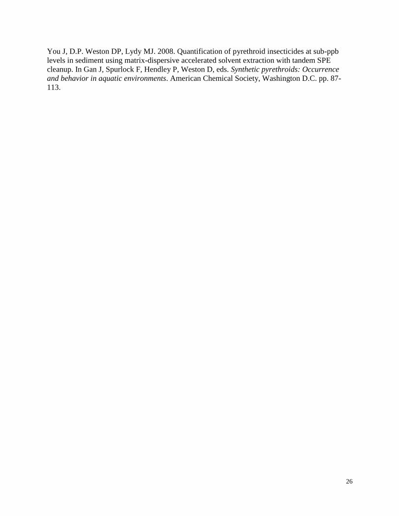
26
You J, D.P. Weston DP, Lydy MJ. 2008. Quantification of pyrethroid insecticides at sub-ppb
levels in sediment using matrix-dispersive accelerated solvent extraction with tandem SPE
cleanup. In Gan J, Spurlock F, Hendley P, Weston D, eds. Synthetic pyrethroids: Occurrence
and behavior in aquatic environments. American Chemical Society, Washington D.C. pp. 87-
113.
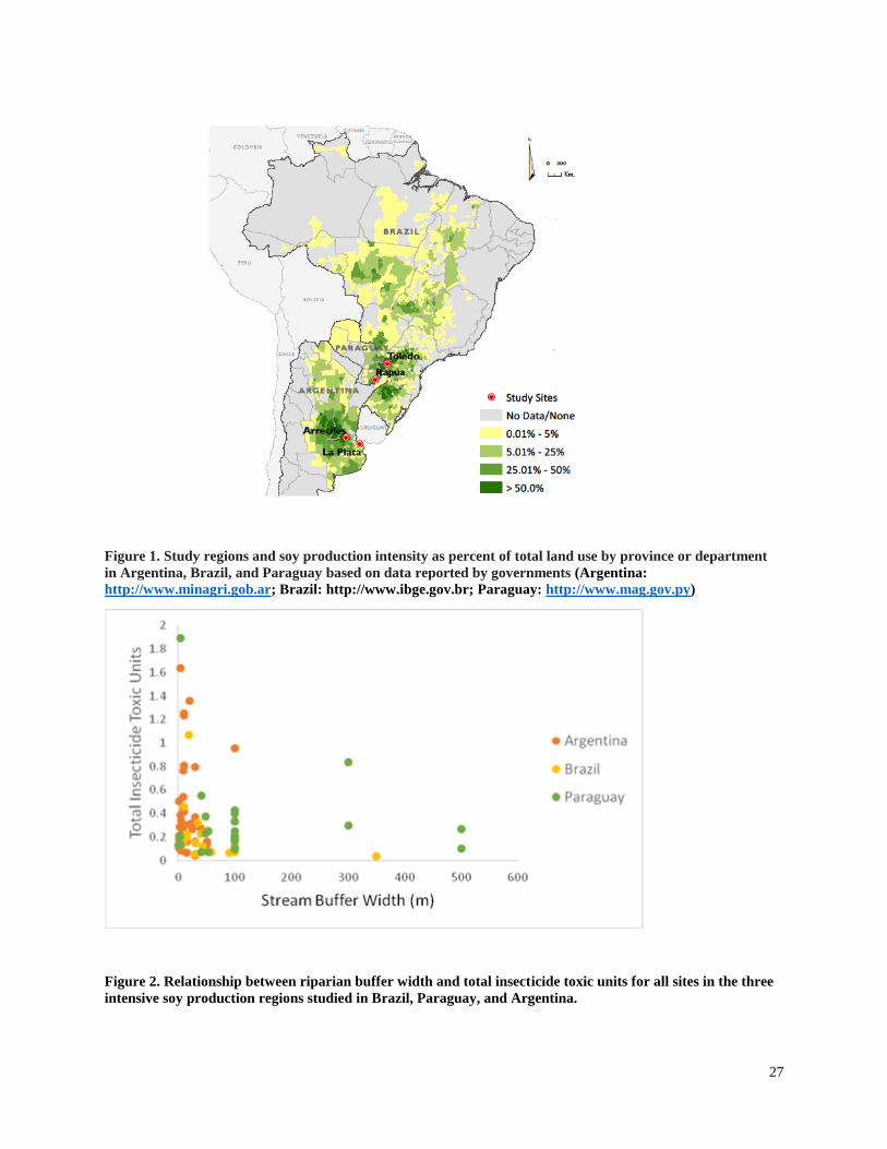
27
Figure 1. Study regions and soy production intensity as percent of total land use by province or department
in Argentina, Brazil, and Paraguay based on data reported by governments (Argentina:
http://www.minagri.gob.ar; Brazil: http://www.ibge.gov.br; Paraguay: http://www.mag.gov.py)
Figure 2. Relationship between riparian buffer width and total insecticide toxic units for all sites in the three
intensive soy production regions studied in Brazil, Paraguay, and Argentina.

Table 1
Sediment concentrations of the most heavily used insecticides, by sampling event. Mean and standard deviation values were calculated by assigning a
value of half the QL for non-detect results and for detections below the QL.
Region and Date La Plata Arrecifes Paraguay Brazil
Dec 2011 Mar
2012
Apr
2012
Jan
2012
Mar
2012
Apr
2012
Feb
2013
Feb
2014
Jan 2013a Dec 2013 Nov 2013
Method
GC-ECD GC-
ECD
GC-
ECD
GC-
ECD
GC-
ECD
GC-
ECD
GC/
MS
GC/
MS
GC-ECD
and GC/MS
GC/MS GC/MS
Quantitation limit (ng/g dw) 0.5 0.5 0.5 0.5 0.5 0.5 0.25 0.25 0.5
(GC-ECD)
0.25 0.25
0.25
(GC/MS)
Number of samplesb 7 7c 4 6 7 5 12d 10e 8f (GC-
ECD)
14g 18h
8b (GC/MS)
Chlorpyrifos koci
995 -
31,000
% samples >
0.5 ng/g dw
29% 57% 100% 86% 100% 20% 100% 75% 56% 77% 83%
Maximum
(ng/g dw)
4.88 7.41 1.42 2.67 3.56 2.02 2.50 2.61 1.26 1.24 1.47
Mean ± sd
(ng/g dw)
1.21 ± 1.79 2.67 ±
2.89
0.92 ±
0.34
1.35 ±
0.83
1.94 ±
0.98
0.69 ±
0.88
1.26 ±
0.54
0.87 ±
0.71
0.50 ± 0.27 0.68 ±
0.26
0.72 ± 0.32
Endosulfan 350 -
19,953
% samples >
0.5 ng/g dw
29%
14%
0%
57%
43%
60%
8%
25%
13%
0%
0%
Maximum
(ng/g dw)
31.88 4.05 - 1.37 2.12 1.42 1.05 4.42 0.85 0.25 0.49
Mean ± sd
(ng/g dw)
7.71 ±
13.13
0.79 ±
1.44
- 0.69 ±
0.44
0.85 ±
0.84
0.66 ±
0.55
0.19 ±
0.27
0.33 ±
0.37
0.26 ± 0.19 0.13 ±
0.04
0.14 ± 0.09
Endosulfan
Sulfate
320,000 % samples
>0.5 ng/g dw
29% 14% 0% 29% 57% 40% 58% 33% 6% 8% 0%
28
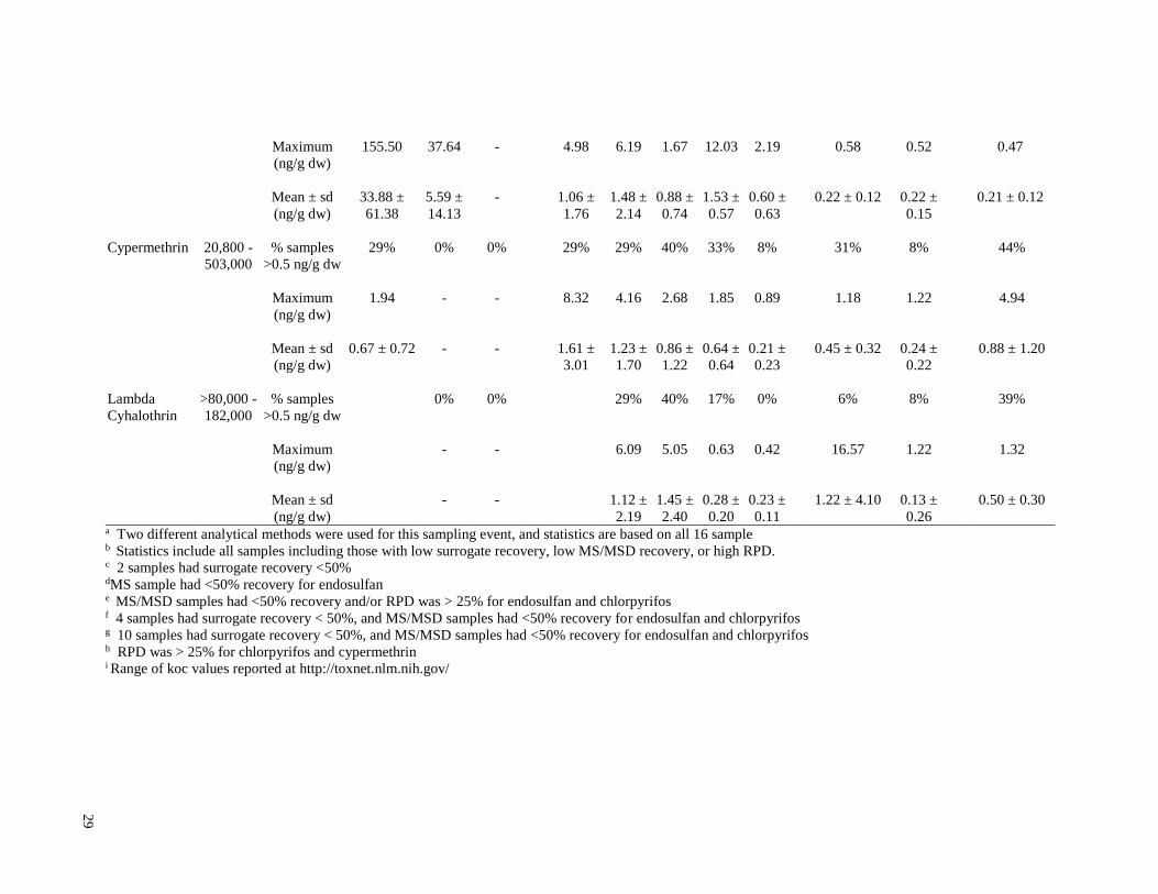
a Two different analytical methods were used for this sampling event, and statistics are based on all 16 sample b Statistics include all samples including those with low surrogate recovery, low MS/MSD recovery, or high RPD. c 2 samples had surrogate recovery <50% dMS sample had <50% recovery for endosulfan e MS/MSD samples had <50% recovery and/or RPD was > 25% for endosulfan and chlorpyrifos f 4 samples had surrogate recovery < 50%, and MS/MSD samples had <50% recovery for endosulfan and chlorpyrifos g 10 samples had surrogate recovery < 50%, and MS/MSD samples had <50% recovery for endosulfan and chlorpyrifos h RPD was > 25% for chlorpyrifos and cypermethrin i Range of koc values reported at http://toxnet.nlm.nih.gov/
Maximum
(ng/g dw)
155.50 37.64 - 4.98 6.19 1.67 12.03 2.19 0.58 0.52 0.47
Mean ± sd
(ng/g dw)
33.88 ±
61.38
5.59 ±
14.13
- 1.06 ±
1.76
1.48 ±
2.14
0.88 ±
0.74
1.53 ±
0.57
0.60 ±
0.63
0.22 ± 0.12 0.22 ±
0.15
0.21 ± 0.12
Cypermethrin 20,800 -
503,000
% samples
>0.5 ng/g dw
29% 0% 0% 29% 29% 40% 33% 8% 31% 8% 44%
Maximum
(ng/g dw)
1.94 - - 8.32 4.16 2.68 1.85 0.89 1.18 1.22 4.94
Mean ± sd
(ng/g dw)
0.67 ± 0.72 - - 1.61 ±
3.01
1.23 ±
1.70
0.86 ±
1.22
0.64 ±
0.64
0.21 ±
0.23
0.45 ± 0.32 0.24 ±
0.22
0.88 ± 1.20
Lambda
Cyhalothrin
>80,000 -
182,000
% samples
>0.5 ng/g dw
0% 0% 29% 40% 17% 0% 6% 8% 39%
Maximum
(ng/g dw)
- - 6.09 5.05 0.63 0.42 16.57 1.22 1.32
Mean ± sd
(ng/g dw)
- - 1.12 ±
2.19
1.45 ±
2.40
0.28 ±
0.20
0.23 ±
0.11
1.22 ± 4.10 0.13 ±
0.26
0.50 ± 0.30
29
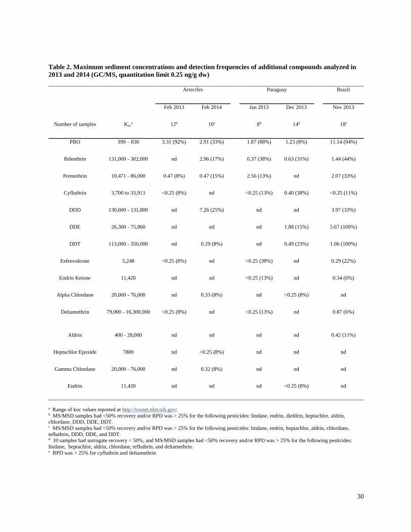
30
Table 2. Maximum sediment concentrations and detection frequencies of additional compounds analyzed in
2013 and 2014 (GC/MS, quantitation limit 0.25 ng/g dw)
a Range of koc values reported at http://toxnet.nlm.nih.gov/
b MS/MSD samples had <50% recovery and/or RPD was > 25% for the following pesticides: lindane, endrin, dieldrin, heptachlor, aldrin, chlordane, DDD, DDE, DDT. c MS/MSD samples had <50% recovery and/or RPD was > 25% for the following pesticides: lindane, endrin, heptachlor, aldrin, chlordane,
tefluthrin, DDD, DDE, and DDT. d 10 samples had surrogate recovery < 50%, and MS/MSD samples had <50% recovery and/or RPD was > 25% for the following pesticides:
lindane, heptachlor, aldrin, chlordane, tefluthrin, and deltamethrin. e RPD was > 25% for cyfluthrin and deltamethrin
Arrecifes Paraguay Brazil
Feb 2013 Feb 2014 Jan 2013 Dec 2013 Nov 2013
Number of samples Koca 12b 10c 8b 14d 18e
PBO 399 – 830 3.31 (92%) 2.91 (33%) 1.87 (88%) 1.23 (8%) 11.14 (94%)
Bifenthrin 131,000 - 302,000 nd 2.96 (17%) 0.37 (38%) 0.63 (31%) 1.44 (44%)
Permethrin 10,471 - 86,000 0.47 (8%) 0.47 (15%) 2.56 (13%) nd 2.07 (33%)
Cyfluthrin 3,700 to 33,913 <0.25 (8%) nd <0.25 (13%) 0.40 (38%) <0.25 (11%)
DDD 130,600 - 131,800 nd 7.26 (25%) nd nd 3.97 (33%)
DDE 26,300 - 75,860 nd nd nd 1.88 (15%) 5.67 (100%)
DDT 113,000 - 350,000 nd 0.29 (8%) nd 0.49 (23%) 1.06 (100%)
Esfenvalerate 5,248 <0.25 (8%) nd <0.25 (38%) nd 0.29 (22%)
Endrin Ketone 11,420 nd nd <0.25 (13%) nd 0.34 (6%)
Alpha Chlordane 20,000 - 76,000 nd 0.33 (8%) nd <0.25 (8%) nd
Deltamethrin 79,000 - 16,300,000
<0.25 (8%) nd <0.25 (13%) nd 0.87 (6%)
Aldrin 400 - 28,000 nd nd nd nd 0.42 (11%)
Heptachlor Epoxide 7800 nd <0.25 (8%) nd nd nd
Gamma Chlordane 20,000 - 76,000 nd 0.32 (8%) nd nd nd
Endrin 11,420 nd nd nd <0.25 (8%) nd
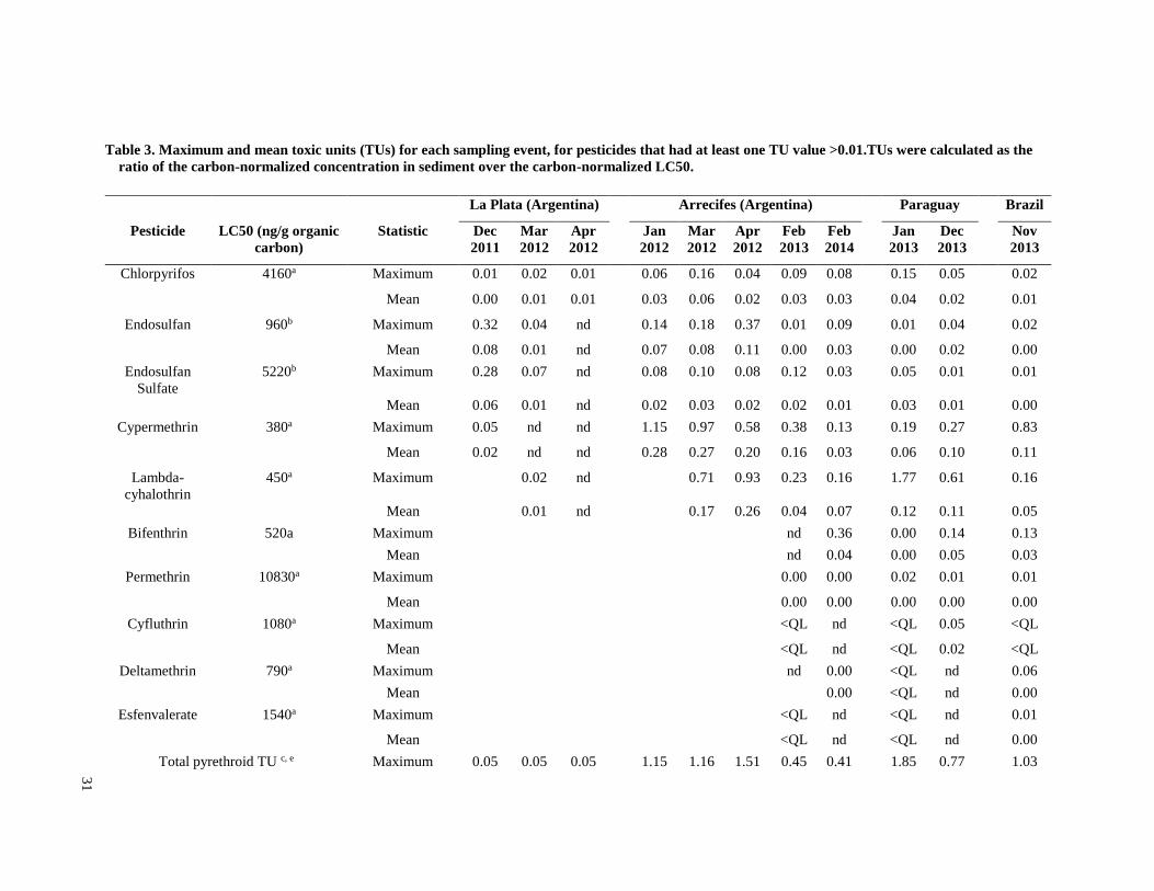
Table 3. Maximum and mean toxic units (TUs) for each sampling event, for pesticides that had at least one TU value >0.01.TUs were calculated as the
ratio of the carbon-normalized concentration in sediment over the carbon-normalized LC50.
La Plata (Argentina) Arrecifes (Argentina) Paraguay Brazil
Pesticide LC50 (ng/g organic
carbon)
Statistic Dec
2011
Mar
2012
Apr
2012
Jan
2012
Mar
2012
Apr
2012
Feb
2013
Feb
2014
Jan
2013
Dec
2013
Nov
2013
Chlorpyrifos 4160a Maximum 0.01 0.02 0.01 0.06 0.16 0.04 0.09 0.08 0.15 0.05 0.02
Mean 0.00 0.01 0.01 0.03 0.06 0.02 0.03 0.03 0.04 0.02 0.01
Endosulfan 960b Maximum 0.32 0.04 nd 0.14 0.18 0.37 0.01 0.09 0.01 0.04 0.02
Mean 0.08 0.01 nd 0.07 0.08 0.11 0.00 0.03 0.00 0.02 0.00
Endosulfan
Sulfate
5220b Maximum 0.28 0.07 nd 0.08 0.10 0.08 0.12 0.03 0.05 0.01 0.01
Mean 0.06 0.01 nd 0.02 0.03 0.02 0.02 0.01 0.03 0.01 0.00
Cypermethrin 380a Maximum 0.05 nd nd 1.15 0.97 0.58 0.38 0.13 0.19 0.27 0.83
Mean 0.02 nd nd 0.28 0.27 0.20 0.16 0.03 0.06 0.10 0.11
Lambda-
cyhalothrin
450a Maximum 0.02 nd 0.71 0.93 0.23 0.16 1.77 0.61 0.16
Mean 0.01 nd 0.17 0.26 0.04 0.07 0.12 0.11 0.05
Bifenthrin 520a Maximum nd 0.36 0.00 0.14 0.13
Mean nd 0.04 0.00 0.05 0.03
Permethrin 10830a Maximum 0.00 0.00 0.02 0.01 0.01
Mean 0.00 0.00 0.00 0.00 0.00
Cyfluthrin 1080a Maximum <QL nd <QL 0.05 <QL
Mean <QL nd <QL 0.02 <QL
Deltamethrin 790a Maximum nd 0.00 <QL nd 0.06
Mean 0.00 <QL nd 0.00
Esfenvalerate 1540a Maximum <QL nd <QL nd 0.01
Mean <QL nd <QL nd 0.00
Total pyrethroid TU c, e Maximum 0.05 0.05 0.05 1.15 1.16 1.51 0.45 0.41 1.85 0.77 1.03
31
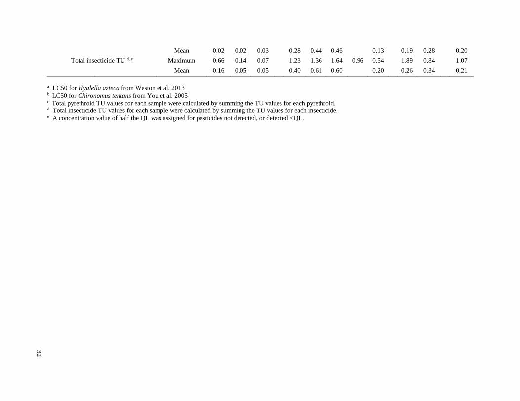
Mean 0.02 0.02 0.03 0.28 0.44 0.46 0.13 0.19 0.28 0.20
Total insecticide TU d, e Maximum 0.66 0.14 0.07 1.23 1.36 1.64 0.96 0.54 1.89 0.84 1.07
Mean 0.16 0.05 0.05 0.40 0.61 0.60 0.20 0.26 0.34 0.21
a LC50 for Hyalella azteca from Weston et al. 2013 b LC50 for Chironomus tentans from You et al. 2005 c Total pyrethroid TU values for each sample were calculated by summing the TU values for each pyrethroid. d Total insecticide TU values for each sample were calculated by summing the TU values for each insecticide. e A concentration value of half the QL was assigned for pesticides not detected, or detected <QL.
32
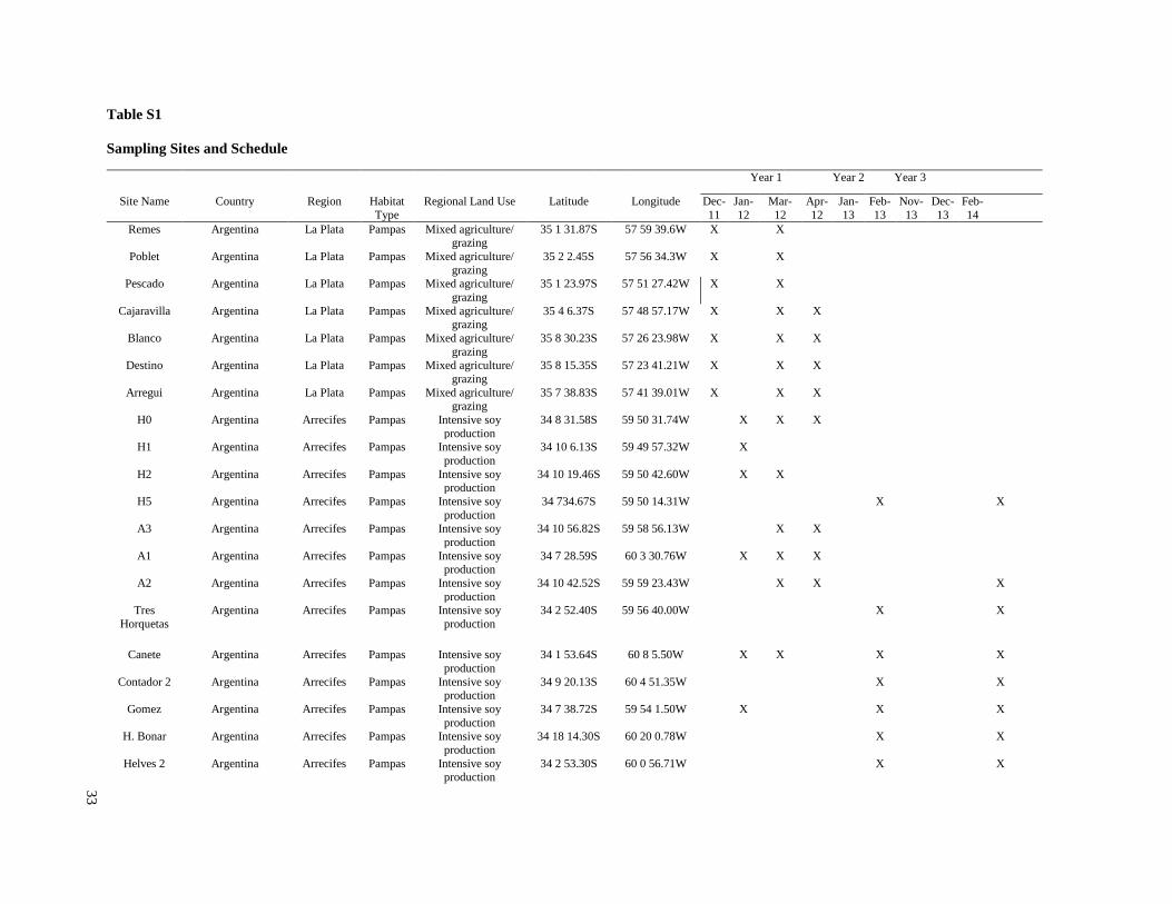
Table S1
Sampling Sites and Schedule
Year 1 Year 2 Year 3
Site Name Country Region Habitat
Type
Regional Land Use Latitude Longitude Dec-
11
Jan-
12
Mar-
12
Apr-
12
Jan-
13
Feb-
13
Nov-
13
Dec-
13
Feb-
14
Remes Argentina La Plata Pampas Mixed agriculture/ grazing
35 1 31.87S 57 59 39.6W X X
Poblet Argentina La Plata Pampas Mixed agriculture/
grazing
35 2 2.45S 57 56 34.3W X X
Pescado Argentina La Plata Pampas Mixed agriculture/
grazing
35 1 23.97S 57 51 27.42W X X
Cajaravilla Argentina La Plata Pampas Mixed agriculture/ grazing
35 4 6.37S 57 48 57.17W X X X
Blanco Argentina La Plata Pampas Mixed agriculture/
grazing
35 8 30.23S 57 26 23.98W X X X
Destino Argentina La Plata Pampas Mixed agriculture/
grazing
35 8 15.35S 57 23 41.21W X X X
Arregui Argentina La Plata Pampas Mixed agriculture/ grazing
35 7 38.83S 57 41 39.01W X X X
H0 Argentina Arrecifes Pampas Intensive soy
production
34 8 31.58S 59 50 31.74W X X X
H1 Argentina Arrecifes Pampas Intensive soy
production
34 10 6.13S 59 49 57.32W X
H2 Argentina Arrecifes Pampas Intensive soy production
34 10 19.46S 59 50 42.60W X X
H5 Argentina Arrecifes Pampas Intensive soy
production
34 734.67S 59 50 14.31W X X
A3 Argentina Arrecifes Pampas Intensive soy
production
34 10 56.82S 59 58 56.13W X X
A1 Argentina Arrecifes Pampas Intensive soy production
34 7 28.59S 60 3 30.76W X X X
A2 Argentina Arrecifes Pampas Intensive soy
production
34 10 42.52S 59 59 23.43W X X X
Tres
Horquetas
Argentina Arrecifes Pampas Intensive soy
production
34 2 52.40S 59 56 40.00W X X
Canete Argentina Arrecifes Pampas Intensive soy
production
34 1 53.64S 60 8 5.50W X X X X
Contador 2 Argentina Arrecifes Pampas Intensive soy production
34 9 20.13S 60 4 51.35W X X
Gomez Argentina Arrecifes Pampas Intensive soy
production
34 7 38.72S 59 54 1.50W X X X
H. Bonar Argentina Arrecifes Pampas Intensive soy
production
34 18 14.30S 60 20 0.78W X X
Helves 2 Argentina Arrecifes Pampas Intensive soy production
34 2 53.30S 60 0 56.71W X X
33

Las Animas Argentina Arrecifes Pampas Intensive soy
production
34 6 59.39S 60 12 32.90W X X
Los Ingleses Argentina Arrecifes Pampas Intensive soy
production
33 59 10.67S 60 11 59.21W X X
Luna 2 Argentina Arrecifes Pampas Intensive soy production
34 11 54.76S 60 1 31.78W X
Maguire Argentina Arrecifes Pampas Intensive soy
production
33 55 19.70S 60 16 5.90W X X X X X
Salto 2 Argentina Arrecifes Pampas Intensive soy
production
34 11 11.90S 60 14 7.22W X X
BR-02 Brazil Toledo Atlantic forest
Intensive soy production
24 48 44.4S 53 42 31.6W X
BR-03 Brazil Toledo Atlantic
forest
Intensive soy
production
24 48 51.4S 53 38 22.2W X
BR-07 Brazil Toledo Atlantic
forest
Intensive soy
production
24 57 31.2S 53 40 53.5W X
BR-10 Brazil Toledo Atlantic forest
Intensive soy production
24 56 54.4S 53 41 52.5W X
BR-11 Brazil Toledo Atlantic
forest
Intensive soy
production
24 56 31.8S 53 42 49.1W X
BR-12 Brazil Toledo Atlantic
forest
Intensive soy
production
24 45 49.1S 53 48 55.7W X
BR-13 Brazil Toledo Atlantic forest
Intensive soy production
24 44 41.6S 53 51 40.3W X
BR-14 Brazil Toledo Atlantic
forest
Intensive soy
production
24 44 40.8S 53 51 59.3W X
BR-15 Brazil Toledo Atlantic
forest
Intensive soy
production
24 45 28.2S 53 52 55.8W X
BR-16 Brazil Toledo Atlantic
forest
Intensive soy
production
24 45 05.2S 53 53 03.6W X
BR-17 Brazil Toledo Atlantic forest
Intensive soy production
24 44 57.4S 53 54 18.2W X
BR-18 Brazil Toledo Atlantic
forest
Intensive soy
production
24 47 43.0S 53 54 11.0W X
BR-19 Brazil Toledo Atlantic
forest
Intensive soy
production
24 49 19.8S 53 54 12.2W X
BR-20 Brazil Toledo Atlantic forest
Intensive soy production
24 49 07.5S 53 50 29.2W X
BR-21 Brazil Toledo Atlantic
forest
Intensive soy
production
24 48 29.6S 53 45 44.8W X
BR-22 Brazil Toledo Atlantic
forest
Intensive soy
production
24 45 48.2S 53 37 54.1W X
BR-23 Brazil Toledo Atlantic forest
Intensive soy production
24 47 48.0S 53 36 16.8W X
BR-24 Brazil Toledo Atlantic
forest
Intensive soy
production
24 47 57.2S 53 36 01.7W X
SD 01 Paraguay Itapua Atlantic
forest
Intensive soy
production
26 42 21.2S 55 31 49.1 W X X
SD 02 Paraguay Itapua Atlantic forest
Intensive soy production
26 45 48.7S 55 33 34.7W X
34
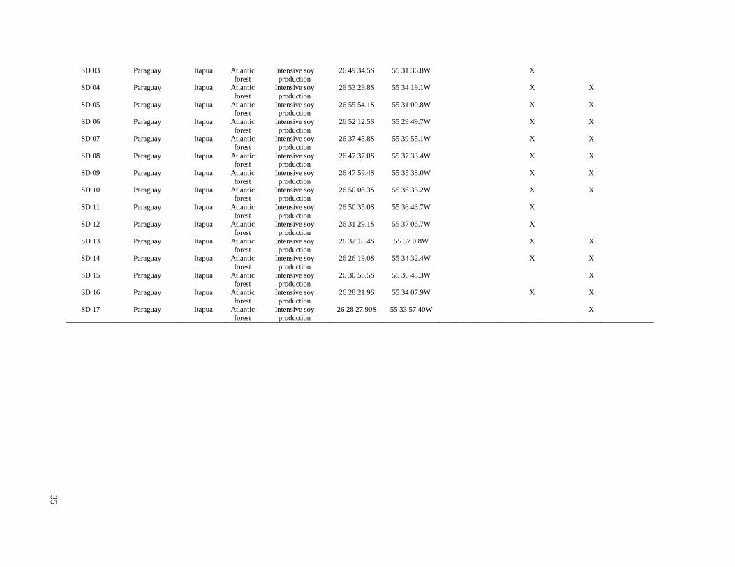
SD 03 Paraguay Itapua Atlantic
forest
Intensive soy
production
26 49 34.5S 55 31 36.8W X
SD 04 Paraguay Itapua Atlantic
forest
Intensive soy
production
26 53 29.8S 55 34 19.1W X X
SD 05 Paraguay Itapua Atlantic forest
Intensive soy production
26 55 54.1S 55 31 00.8W X X
SD 06 Paraguay Itapua Atlantic
forest
Intensive soy
production
26 52 12.5S 55 29 49.7W X X
SD 07 Paraguay Itapua Atlantic
forest
Intensive soy
production
26 37 45.8S 55 39 55.1W X X
SD 08 Paraguay Itapua Atlantic forest
Intensive soy production
26 47 37.0S 55 37 33.4W X X
SD 09 Paraguay Itapua Atlantic
forest
Intensive soy
production
26 47 59.4S 55 35 38.0W X X
SD 10 Paraguay Itapua Atlantic
forest
Intensive soy
production
26 50 08.3S 55 36 33.2W X X
SD 11 Paraguay Itapua Atlantic forest
Intensive soy production
26 50 35.0S 55 36 43.7W X
SD 12 Paraguay Itapua Atlantic
forest
Intensive soy
production
26 31 29.1S 55 37 06.7W X
SD 13 Paraguay Itapua Atlantic
forest
Intensive soy
production
26 32 18.4S 55 37 0.8W X X
SD 14 Paraguay Itapua Atlantic forest
Intensive soy production
26 26 19.0S 55 34 32.4W X X
SD 15 Paraguay Itapua Atlantic
forest
Intensive soy
production
26 30 56.5S 55 36 43.3W X
SD 16 Paraguay Itapua Atlantic
forest
Intensive soy
production
26 28 21.9S 55 34 07.9W X X
SD 17 Paraguay Itapua Atlantic
forest
Intensive soy
production
26 28 27.90S 55 33 57.40W X
35
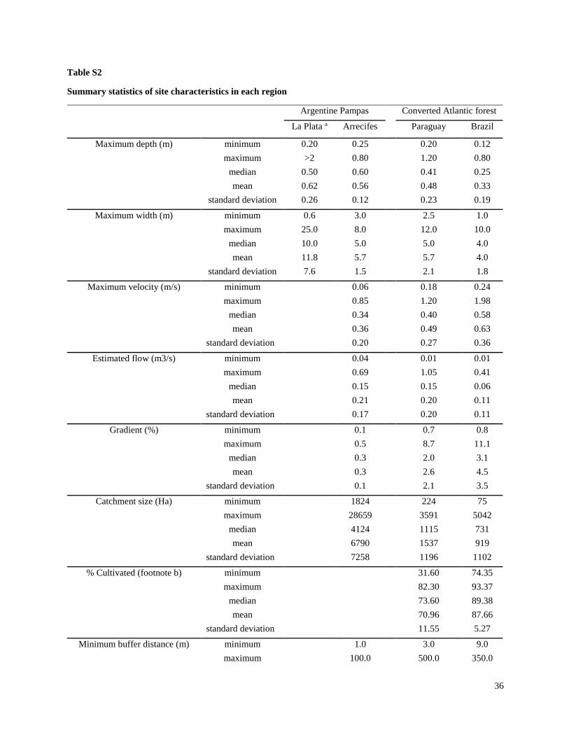
36
Table S2
Summary statistics of site characteristics in each region
Argentine Pampas Converted Atlantic forest
La Plata a Arrecifes Paraguay Brazil
Maximum depth (m) minimum 0.20 0.25 0.20 0.12
maximum >2 0.80 1.20 0.80
median 0.50 0.60 0.41 0.25
mean 0.62 0.56 0.48 0.33
standard deviation 0.26 0.12 0.23 0.19
Maximum width (m) minimum 0.6 3.0 2.5 1.0
maximum 25.0 8.0 12.0 10.0
median 10.0 5.0 5.0 4.0
mean 11.8 5.7 5.7 4.0
standard deviation 7.6 1.5 2.1 1.8
Maximum velocity (m/s) minimum 0.06 0.18 0.24
maximum 0.85 1.20 1.98
median 0.34 0.40 0.58
mean 0.36 0.49 0.63
standard deviation 0.20 0.27 0.36
Estimated flow (m3/s) minimum 0.04 0.01 0.01
maximum 0.69 1.05 0.41
median 0.15 0.15 0.06
mean 0.21 0.20 0.11
standard deviation 0.17 0.20 0.11
Gradient (%) minimum 0.1 0.7 0.8
maximum 0.5 8.7 11.1
median 0.3 2.0 3.1
mean 0.3 2.6 4.5
standard deviation 0.1 2.1 3.5
Catchment size (Ha) minimum 1824 224 75
maximum 28659 3591 5042
median 4124 1115 731
mean 6790 1537 919
standard deviation 7258 1196 1102
% Cultivated (footnote b) minimum 31.60 74.35
maximum 82.30 93.37
median 73.60 89.38
mean 70.96 87.66
standard deviation 11.55 5.27
Minimum buffer distance (m) minimum 1.0 3.0 9.0
maximum 100.0 500.0 350.0

37
median 10.0 100.0 32.5
mean 19.7 89.3 56.6
standard deviation 23.0 93.4 87.3
Water conductivity (uS/cm) minimum 220 663 24 14
maximum 4000 1796 163 61
median 921 895 61 28
mean 906 961 66 31
standard deviation 813 247 24 13
Water temperature (C) minimum 18.3 17.6 19.0
maximum 30.5 24.0 22.8
median 22.9 21.0 20.7
mean 23.1 20.7 20.6
standard deviation 3.0 1.4 1.0
Water pH minimum 6.7 7.0 5.9 4.5
maximum 9.0 9.1 7.4 7.6
median 7.4 8.0 6.8 6.7
mean 7.7 7.9 6.8 6.6
standard deviation 0.7 0.5 0.3 0.7
Dissolved oxygen (mg/L) minimum 4.00 4.90 2.90 7.30
maximum 12.90 18.77 10.00 14.60
median 9.30 10.27 8.42 8.50
mean 8.48 10.78 8.37 8.79
standard deviation 2.6 3.2 1.0 1.3
Water turbidity minimum 3.9 5.5 3.2
maximum 96.0 37.5 31.0
median 14.7 11.2 16.1
mean 21.9 13.9 16.8
standard deviation 22.2 6.4 7.1
% sediment TOC minimum 2% 0.26 0.22 1.37
maximum 12% 2.00 2.12 3.24
median 10% 1.16 0.55 2.39
mean 8% 1.16 0.69 2.32
standard deviation 4% 0.52 0.44 0.68
% sediment fines (silt and clay) minimum 52.7 10.6 44.6
maximum 78.1 86.3 83.1
median 64.7 38.6 65.7
mean 65.5 42.0 65.9
standard deviation 8.6 18.7 11.6
a La Plata statistics don't include temperature data because it was only collected for some samples. Other parameters
are blank because measurements were not taken
b Paraguay/Brazil - cultivated area is based on non-forested area, estimated with LANDSAT data
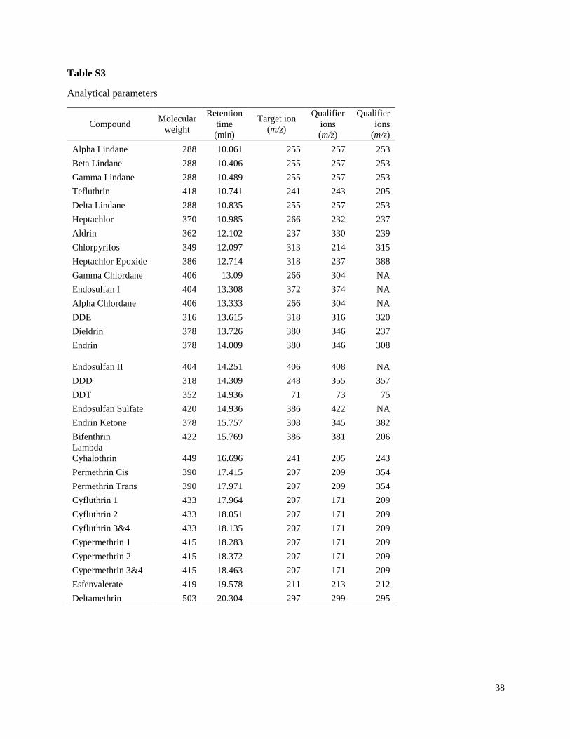
38
Table S3
Analytical parameters
Compound Molecular
weight
Retention
time
(min)
Target ion
(m/z)
Qualifier
ions
(m/z)
Qualifier
ions
(m/z)
Alpha Lindane 288 10.061 255 257 253
Beta Lindane 288 10.406 255 257 253
Gamma Lindane 288 10.489 255 257 253
Tefluthrin 418 10.741 241 243 205
Delta Lindane 288 10.835 255 257 253
Heptachlor 370 10.985 266 232 237
Aldrin 362 12.102 237 330 239
Chlorpyrifos 349 12.097 313 214 315
Heptachlor Epoxide 386 12.714 318 237 388
Gamma Chlordane 406 13.09 266 304 NA
Endosulfan I 404 13.308 372 374 NA
Alpha Chlordane 406 13.333 266 304 NA
DDE 316 13.615 318 316 320
Dieldrin 378 13.726 380 346 237
Endrin 378 14.009 380 346 308
Endosulfan II 404 14.251 406 408
NA
DDD 318 14.309 248 355 357
DDT 352 14.936 71 73 75
Endosulfan Sulfate 420 14.936 386 422 NA
Endrin Ketone 378 15.757 308 345 382
Bifenthrin 422 15.769 386 381 206
Lambda
Cyhalothrin 449 16.696 241 205 243
Permethrin Cis 390 17.415 207 209 354
Permethrin Trans 390 17.971 207 209 354
Cyfluthrin 1 433 17.964 207 171 209
Cyfluthrin 2 433 18.051 207 171 209
Cyfluthrin 3&4 433 18.135 207 171 209
Cypermethrin 1 415 18.283 207 171 209
Cypermethrin 2 415 18.372 207 171 209
Cypermethrin 3&4 415 18.463 207 171 209
Esfenvalerate 419 19.578 211 213 212
Deltamethrin 503 20.304 297 299 295

39
CHAPTER 3
Acute toxicity of four insecticides to the South American amphipod Hyalella curvispina
based on sediment and water exposures
40
Acute toxicity of four insecticides to the South American amphipod Hyalella curvispina
based on sediment and water exposures
Abstract
Cypermethrin, lambda-cyhalothrin, chlorpyrifos, and endosulfan are insecticides with very high
aquatic toxicity that are commonly used in soy production and other large scale crop systems in
South America. For each of these insecticides, in both sediment and water, we determined
median lethal concentration (LC50) values for Hyalella curvispina, a freshwater amphipod that is
widespread in South America and is closely related to H. azteca, a standard test species in the
United States. We then calculated species sensitivity distributions (SSDs) for freshwater
invertebrate taxa using results of this study and other available data. Results of sediment and
water toxicity tests were consistent, with the lowest L50 values for lambda-cyhalothrin, followed
by cypermethrin, chlorpyrifos and alpha-endosulfan. Although the younger age class of neonates
(1-2 wks) was more sensitive to both pyrethroid insecticides than the older age class (2-3 wks),
the younger age class was less practical for bioassays because of high variability in control
survival and difficulty finding live organisms when terminating sediment tests. The SSD
resultsfor the four pesticides tested indicated that the sensitivity of H. curvispina is similar to that
of H. azteca, and that both organisms are more sensitive than most other freshwater invertebrate
taxa.
Introduction
Cypermethrin, lambda-cyhalothrin, chlorpyrifos and endosulfan are insecticides with very high
aquatic toxicity that are commonly used in soy production and other large scale crop systems in
South America(Hunt et al., 2016). In recent years, soybean production has become a major
export crop for multiple countries in South America, including Brazil, Argentina, Paraguay,
Uruguay, and Bolivia (Castanheira and Freire, 2013; Garrett et al., 2013). Lepidoptera pests are
often controlled by applications of chorpyrifos, an organophosphate, and Hemiptera pests by
endosulfan, an organochlorine. Pyrethroids, especially cypermethrin and lambda-cyhalothrin, are
commonly used for both types of pests, and are often applied at the same time as other pesticides
(Di Marzio et al., 2010; Organismo Provincial para el Desarrollo Sostenible, 2013). Multiple
studies have found high detection rates of these pesticides in both sediment and water in South
American streams, at concentrations that are toxic to aquatic organisms (Di Marzio et al., 2010;
Hunt et al., 2016; Jergentz et al., 2004b; Marino and Ronco, 2005; Mugni et al., 2011; Possavatz
et al., 2014).
As insecticides are increasingly used in South America and other parts of the southern
hemisphere, the question has arisen as to whether water quality standards based on toxicity data
for northern hemisphere taxa are adequately protective. The vast majority of aquatic toxicity
testing for pesticides is performed on species from Europe and North America, and toxicity data
for species native to the southern hemisphere are lacking. For example, Hagen and Douglas
(2014) compiled laboratory toxicity data to compare sensitivity of Australian marine
invertebrates to northern hemisphere species, and found sufficient data to compare only three out
of 109 chemical substances.
Hyalella curvispina is a freshwater amphipod that is widespread in South America, and it has
been utilized in toxicity testing for over a decade, but more data are needed to establish pesticide
toxicity threshold values for this species. Another species of the same genus, H. azteca, is native
41
to North America and is a standard test species in the United States (United States Environmental
Protection Agency, 2000). H. azteca is known to be very sensitive to many pesticides including
pyrethroids and chlorpyrifos, therefore it is often used in aquatic toxicity testing when these
pesticides are expected to be present in water bodies (Weston et al., 2009). Hyalella species are
especially useful in toxicity testing because they can be used in both sediment and water toxicity
tests (United States Environmental Protection Agency, 2000; Weston and Lydy, 2010).
The insecticides most commonly used in soy production in South America (chlorpyrifos,
endosulfan, cypermethrin, and lambda-cyhalothrin) have low water solubility, and a high affinity
to bind to soil and sediments based on chemical properties (Hunt et al., 2016). Sediment LC50
values for H. azteca have been published for all four of these insecticides (Weston et al., 2013;
You et al., 2004), and freshwater LC50 values for H. azteca have been published for three of
them (Ding et al., 2012; Wan et al., 2005; Donald P. Weston et al., 2013). However, no sediment
LC50 values have been published for H. curvispina, although previous studies have published
LC50 values for some insecticides in water(Mugni et al., 2013, 2012).
To utilize H. curvispina as a sensitive surrogate species in pesticide toxicity testing, it is
important to determine the most sensitive life stage that can be used in bioassays. H. azteca
toxicity tests are generally conducted with neonates that are between 7-14 days old when tests are
started because this life stage has been demonstrated to be more sensitive than older ones in
testing of a limited number of toxicants (United States Environmental Protection Agency, 2000).
However, many published studies on H. curvispina toxicity testing have used juveniles or adults
(Mugni et al., 2013, 2012, 2011).
The objectives of this study were to: (1) establish LC50 values for H. curvispina for the
chlorpyrifos, alpha-endosulfan, cypermethrin, and lambda-cyaholothrin in both sediment and
water; (2) compare the sensitivity of H. curvispina to H. azteca and other freshwater aquatic
invertebrates; and (3) compare the sensitivity of different ages groups of H. curvispina, and
evaluate their practicality for use in bioassays.
Materials and Methods
Test materials
H. curvispina was collected from the El Destino stream in a relatively undeveloped area located
in a reserve 25 km south of the city of La Plata, Argentina. Organisms were acclimated for at
least one week prior to use in bioassays. They were cultured in plastic containers filled with
reconstituted water prepared according to recommendations for H. azteca (United States
Environmental Protection Agency, 2000). Lettuce leaves were placed in culture containers to
serve as substrate and food, supplemented by formulated fish food every two days.
Sediment was collected from the same location as H. curvispina collection, and thoroughly
homogenized prior to taking an aliquot for analysis of insecticides. None of the insecticides
analyzed (chlopyrifos, endosulfan, cypermethrin and lambda-cyhalothrin) were detected in
sediment samples. Organic carbon content was 1.7%, and moisture content measured just prior to
spiking was 3.6%.
42
Sediment and water toxicity bioassays
The 96 h water and 10 d sediment acute toxicity bioassays generally followed the methods of
Weston et al. (2009) and Weston and Jackson (2009), except for substituting formulated fish
food for yeast/cerophyll/trout chow for the specified feeding regimes (1 feeding at 48 h for water
tests, daily feeding for sediment tests). A 16 h:8 h light:dark photocycle was used, and
temperature was maintained at 23 °C. Five to seven concentration steps were used for each
toxicant, with each step varying by a factor of 2. Spiked sediment samples were prepared
approximately 1 week prior to starting bioassays, and stored in a refrigerator after thorough
homogenization by hand. Spiked water was prepared immediately prior to beginning bioassays.
Each concentration was prepared by adding the appropriate amount of toxicant dissolved in
acetone, with < 32 μL/L acetone in water and < 1.1 μg/g acetone in sediment. Solvent controls
were spiked with the maximum amount of acetone that was used in the concentrations series. For
each pesticide concentration and the control, tests were conducting using three replicate glass
beakers, each containing 10 H. curvispina individuals.
For water bioassays, 80 mL of spiked reconstituted water and a substrate consisting of a 1 cm2
nylon screen was included in each beaker. After 48 h exposure, 1 mL of formulated fish food was
added to each beaker, and a 6 h feeding period was provided. Then ∼80% of the water was
removed from the beaker and replaced with fresh sample. After an additional 48 h (96 h total),
the test was terminated and survivors counted.
To compare sensitivity of different ages, separate water bioassays were conducted for two
groups: (1) organisms that passed through a 500 μm sieve but did not pass through a 355 μm
sieve (i.e. those approximately 1-2 weeks old); and (2) organisms that passed through a 710 μm
sieve but did not pass through a 500 μm sieve (i.e. approximately 2-3 weeks old). An additional
size class (organisms that did not pass through a 710 μm sieve, and were greater than 3 weeks
old) was tested for lambda-cyhalothrin. Organisms were sieved 3 – 5 d prior to initiating
bioassays.
For sediment bioassays, 70g of spiked sediment and 200 mL of reconstituted water were added to
each beaker. We selected test organisms that passed through a 710 μm sieve but did not pass
through a 355 μm sieve (i.e. approximately 1-3 weeks old). Organisms were sieved 5-6 d prior to
initiating bioassays. Twice a day 80% of the water was removed from the beaker and replaced
with fresh reconstituted water. 1 mL of formulated fish food was added to each beaker daily just
after the first water change.
Mortality data were used to estimate the LC50 values and 95% confidence intervals by probit
analysis using the USEPA Benchmark Dose Software (USEPA 2015).
Species Sensitivity Distributions
To compare the sensitivity of H. curvispinato sensitivities of H. azteca and other aquatic
invertebrate taxa, we calculated species sensitivity distributions (SSDs) for each insecticide,
using the United States Environmental Protection Agency (USEPA) SSD Generator software
(United States Environmental Protection Agency, 2015a). SSDs use available toxicity data for
multiple species tested with a given chemical to derive a joint sensitivity distribution, from which
the proportion of species affected by a certain concentrations can be estimated by the quantile of

43
the distribution (Smetanová et al., 2014). The USEPA SSD Generator software produces SSDs
by fitting the log-probit distribution to toxicity data (United States Environmental Protection
Agency, 2015a)
To calculate SSDs for each insecticide examined in this study, we used LC50 values obtained for
H. curvispina from the present study, as well as all acute (1 to 4d) water toxicity data for
freshwater invertebrates available in the USEPA ECOTOX database, including mortality and
immobilization endpoints (United States Environmental Protection Agency, 2015b). Because
cypermethrin results for H. azteca were not included in the ECOTOX database, we supplemented
the cypermethrin SSD data set with a 4d immobilization EC50 value (Weston and Jackson,
2009).
Only one study in the ECOTOX database reported LC50 values for H. curvispina(Mugni et al.,
2012). Instead of combining data from that study with the present study, we used separate data
points for each the two studies in the SSD. We kept them separate so that we could compare the
relative sensitivities of H. curvispina obtained from our study results with those of Mugni et al.
2012. For all other taxa, results from all studies of the relevant insecticide were combined into a
single data point by using the mean of all reported LC50 values for each taxa for input into the
SSD (United States Environmental Protection Agency, 2015a).
Adequate water toxicity data were available in the ECOTOX database for three of the four
insecticides: 146 taxa had data available for chlorpyrifos, 71 taxa for endosulfan, and 56 taxa for
cypermethrin. For lambda-cyhalothrin, LC50 data were available for only three taxa in addition
to H. curvispina. Therefore, we also calculated a SSD for the insecticide gamma-cyhalothrin, for
which data were available for13 taxa. SSDs were generated only for water toxicity, because
insufficient data were available to calculate SSDs for sediment toxicity.
Results
Acute toxicity to Hyalella curvispina
Results of sediment and water toxicity tests were consistent, with the lowest LC50 values for
lambda-cyhalothrin, followed by cypermethrin, chlorpyrifos, and alpha-endosulfan (Table 1).
Water temperatures measured in all control replicates twice a day ranged between 22.4– 23.9 °C
for water bioassays, and 21.4 – 24.5 °C for sediment bioassays.
The LC50 values for both cypermethrin and lambda-cyahothrin were lower for the smaller size
class, and confidence intervals did not overlap (Table 1). When the largest age class (2-3 weeks
old) was tested with lambda-cyhalothrin in water using the same concentration series as the other
two age classes, there was no significant mortality even at the highest concentration (12 ng/L).
Survival in control replicates for water bioassays using organisms sieved with sizes 500-710 μm
ranged from 90-100%, with a mean of 97 – 100% for each test. For water bioassays using
smaller organisms (sieve size 355-500um), control mortality was higher, with survival rates
ranging from 30-100% for individual replicates and 70-100% for means of all control replicates.
For endosulfan, LC50 values could not be calculated for the younger age class because of high
variability in both controls and dilution series.
44
Species Sensitivity Distributions
The SSD for chlorpyrifos (Figure 1a) indicates that H. curvispina is more sensitive than 94% of
species, based on the H. curvispina LC50 value determined in the present study, and more
sensitive than 96% of species based on the H. curvispina LC50 value determined previously
(Mugni et al., 2012). More sensitive organisms tested include H. azteca, the mayflies
Deleatidium sp. and Procloeon sp.,the cladocerans Daphnia ambigua and Ceriodaphnia dubia,
and the dragonfly Pseudagrion spp. D. ambigua is known to be native to South America, and H.
azteca occurs in just the northernmost part of South America.
The SSD for endosulfan (Figure 1b) indicates that H. curvispina is more sensitive than 56% of
species, based on the H. curvispina LC50 value determined in the present study, and more
sensitive than 78% of species based on the H. curvispina LC50 value determined previously
(Mugni et al., 2012). However, the present study used only the alpha endosulfan isomer, which is
more toxic than the typical endosulfan isomer mixture that was used in the and likely in most
other reported results. H. azteca is more sensitive than 67% of species, based on results from
only one study. Of the 15 species tested that were more sensitive than H. curvispina based on
results of the present study, all were crustaceans except for two mayflies (Atalophlebia australis
and Jappa kutera) and one caddisfly (Cheumatopsyche sp.).
The SSD for cypermethrin (Figure 1c) indicates that H. curvispina is more sensitive than 87% of
species, based on the H. curvispinaLC50 value determined in the present study, and more
sensitive than 89% of speciesbased on the H. curvispina LC50 value determined previously
(Mugni et al., 2012). The4d immobilization EC50 value reported by Weston and Jackson (2009)
indicates that H. azteca is more sensitive than 99% of all species, and was the most sensitive of
all species tested. Taxa that were more sensitive than H. curvispina include the mayfly Baetis
rhodani, the decapods Macrobrachium rosenbergii, Trichodactylus borellianus, and
Palaemonetes argentines, and the chironomid Tanytarsus sp. All of these species belong to
genera that are common in South America.
For lambda-cyhalothrin, LC50 data were available for only three other taxa, and H. curvispina
was more sensitive than all of them (Figure 1d), based on results of the present study. No other
studies included LC50 values for H. curvispina or H. azteca. The SSD estimates that H.
curvispina is more sensitive than 87% of all species. There is high uncertainty in this estimate
given the limited amount of data, but it corresponds well with the SSD generated for gamma-
cyhalothrin (Figure 1e), which indicates that H. azteca is more sensitive than 88% of species
(there were no data available for H. curvispina for this compound).
Discussion
The results of this study indicate that for the four pesticides tested, the sensitivity of H.
curvispina is similar to that of H. azteca, and that both organisms are more sensitive than most
other freshwater invertebrate taxa. Results of this study are also in close agreement with previous
data the sensitivity of H. curvispina, although there were some differences in the methods.
Although for H. azteca bioassays, neonates of 7-14d are recommended for use (United States
Environmental Protection Agency, 2000), we found that it was impractical to use organisms of
H. curvispinaat this young age because of high mortality in controls.
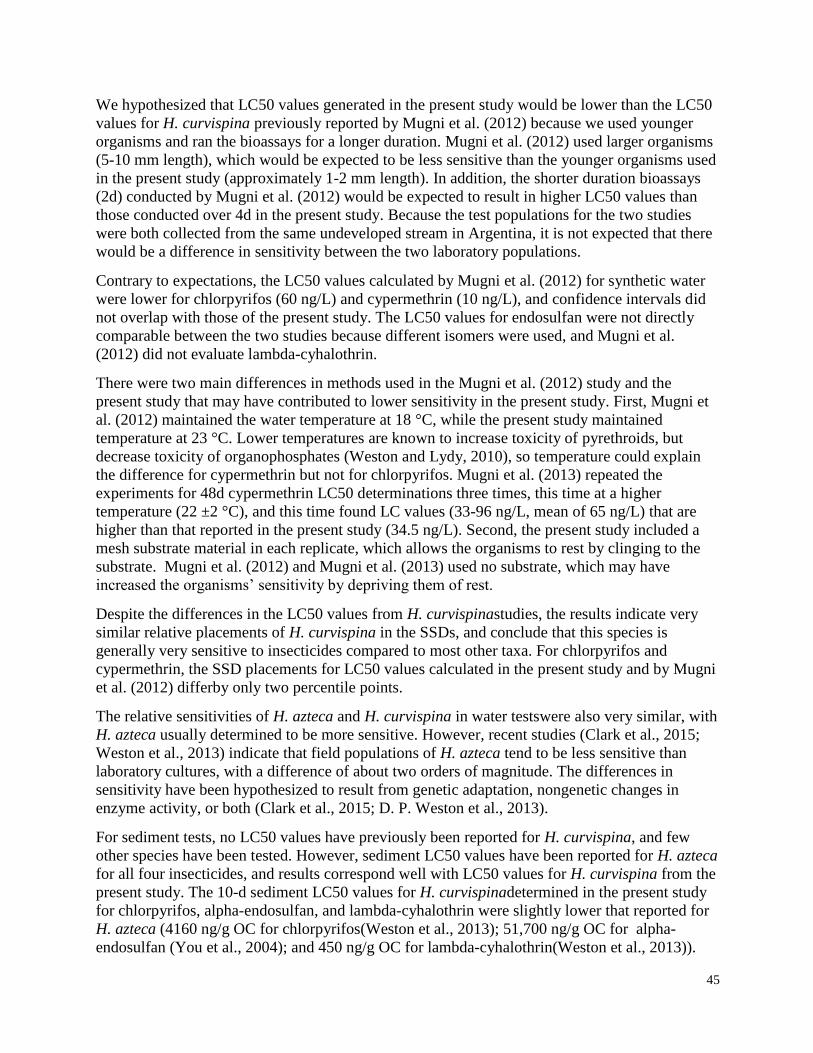
45
We hypothesized that LC50 values generated in the present study would be lower than the LC50
values for H. curvispina previously reported by Mugni et al. (2012) because we used younger
organisms and ran the bioassays for a longer duration. Mugni et al. (2012) used larger organisms
(5-10 mm length), which would be expected to be less sensitive than the younger organisms used
in the present study (approximately 1-2 mm length). In addition, the shorter duration bioassays
(2d) conducted by Mugni et al. (2012) would be expected to result in higher LC50 values than
those conducted over 4d in the present study. Because the test populations for the two studies
were both collected from the same undeveloped stream in Argentina, it is not expected that there
would be a difference in sensitivity between the two laboratory populations.
Contrary to expectations, the LC50 values calculated by Mugni et al. (2012) for synthetic water
were lower for chlorpyrifos (60 ng/L) and cypermethrin (10 ng/L), and confidence intervals did
not overlap with those of the present study. The LC50 values for endosulfan were not directly
comparable between the two studies because different isomers were used, and Mugni et al.
(2012) did not evaluate lambda-cyhalothrin.
There were two main differences in methods used in the Mugni et al. (2012) study and the
present study that may have contributed to lower sensitivity in the present study. First, Mugni et
al. (2012) maintained the water temperature at 18 °C, while the present study maintained
temperature at 23 °C. Lower temperatures are known to increase toxicity of pyrethroids, but
decrease toxicity of organophosphates (Weston and Lydy, 2010), so temperature could explain
the difference for cypermethrin but not for chlorpyrifos. Mugni et al. (2013) repeated the
experiments for 48d cypermethrin LC50 determinations three times, this time at a higher
temperature (22 ±2 °C), and this time found LC values (33-96 ng/L, mean of 65 ng/L) that are
higher than that reported in the present study (34.5 ng/L). Second, the present study included a
mesh substrate material in each replicate, which allows the organisms to rest by clinging to the
substrate. Mugni et al. (2012) and Mugni et al. (2013) used no substrate, which may have
increased the organisms’ sensitivity by depriving them of rest.
Despite the differences in the LC50 values from H. curvispinastudies, the results indicate very
similar relative placements of H. curvispina in the SSDs, and conclude that this species is
generally very sensitive to insecticides compared to most other taxa. For chlorpyrifos and
cypermethrin, the SSD placements for LC50 values calculated in the present study and by Mugni
et al. (2012) differby only two percentile points.
The relative sensitivities of H. azteca and H. curvispina in water testswere also very similar, with
H. azteca usually determined to be more sensitive. However, recent studies (Clark et al., 2015;
Weston et al., 2013) indicate that field populations of H. azteca tend to be less sensitive than
laboratory cultures, with a difference of about two orders of magnitude. The differences in
sensitivity have been hypothesized to result from genetic adaptation, nongenetic changes in
enzyme activity, or both (Clark et al., 2015; D. P. Weston et al., 2013).
For sediment tests, no LC50 values have previously been reported for H. curvispina, and few
other species have been tested. However, sediment LC50 values have been reported for H. azteca
for all four insecticides, and results correspond well with LC50 values for H. curvispina from the
present study. The 10-d sediment LC50 values for H. curvispinadetermined in the present study
for chlorpyrifos, alpha-endosulfan, and lambda-cyhalothrin were slightly lower that reported for
H. azteca (4160 ng/g OC for chlorpyrifos(Weston et al., 2013); 51,700 ng/g OC for alpha-
endosulfan (You et al., 2004); and 450 ng/g OC for lambda-cyhalothrin(Weston et al., 2013)).

46
The 10-d sediment LC50 for H. curvispinadetermined for cypermethrin in the present study was
2073 ng/g OC, higher than that reported for H. azteca (380 ng/g OC (Weston et al. 2013)).
Although the younger age group of H. curvispina was somewhat more sensitive to the pyrethroid
insecticides, organisms of this size were problematic to use in bioassays because of variable
survival in controls. In addition to the variability in controls, we found that it was impractical to
use the younger age category for sediment bioassays because it required many hours to search
through the sediment for the small organisms when terminating bioassays.
This study adds information on pesticide sensitivity of an important South American amphipod
species, and indicates that its sensitivity is very similar to a closely related North America
species. A repeated criticism by the scientific community in South Americais the lack of
sensitivity data on species that occur outside of Europe and North America, and the application
of sensitivity data for northern hemisphere species to South American taxa. There may be reason
to believe that sensitivities could be different in species occurring in the Southern hemisphere
and near the equator. For example, Kwok et al. (2007) found that tropical species may be more
sensitive than temperate species to pesticides, while temperate species are likely to be more
sensitive to metals. More studies are needed on a range of organisms to determine whether use of
sensitivity data for northern hemisphere species are adequately protective for southern
hemisphere species.
References
Castanheira, É.G., Freire, F., 2013. Greenhouse gas assessment of soybean production:
implications of land use change and different cultivation systems. J. Clean. Prod. 54, 49–60.
doi:10.1016/j.jclepro.2013.05.026
Clark, S.L., Ogle, R.S., Gantner, A., Hall, L.W., Mitchell, G., Giddings, J., McCoole, M., Dobbs,
M., Henry, K., Valenti, T., 2015. Comparative sensitivity of field and laboratory populations of
Hyalella azteca to the pyrethroid insecticides bifenthrin and cypermethrin: Hyalella azteca field
and laboratory population sensitivity to pyrethroids. Environ. Toxicol. Chem. 34, 2250–2262.
doi:10.1002/etc.2907
Di Marzio, W.D., Sáenz, M.E., Alberdi, J.L., Fortunato, N., Cappello, V., Montivero, C.,
Ambrini, G., 2010. Environmental impact of insecticides applied on biotech soybean crops in
relation to the distance from aquatic ecosystems. Environ. Toxicol. Chem. n/a–n/a.
doi:10.1002/etc.246
Ding, Y., Landrum, P.F., You, J., Harwood, A.D., Lydy, M.J., 2012. Use of solid phase
microextraction to estimate toxicity: Relating fiber concentrations to toxicity-part I. Environ.
Toxicol. Chem. 31, 2159–2167. doi:10.1002/etc.1935
Garrett, R.D., Rueda, X., Lambin, E.F., 2013. Globalization’s unexpected impact on soybean
production in South America: linkages between preferences for non-genetically modified crops,
eco-certifications, and land use. Environ. Res. Lett. 8, 044055. doi:10.1088/1748-
9326/8/4/044055
Hagen, T.G., Douglas, R.W., 2014. Comparative chemical sensitivity between marine Australian
and Northern Hemisphere ecosystems: Is an uncertainty factor warranted for water-quality-

47
guideline setting?: Australian vs Northern Hemisphere ecosystem sensitivities. Environ. Toxicol.
Chem. 33, 1187–1192. doi:10.1002/etc.2548
Hunt, L., Bonetto, C., Resh, V.H., Buss, D.F., Fanelli, S., Marrochi, N., Lydy, M.J., 2016.
Insecticide concentrations in stream sediments of soy production regions of South America. Sci.
Total Environ. 547, 114–124. doi:10.1016/j.scitotenv.2015.12.140
Jergentz, S., Pessacq, P., Mugni, H., Bonetto, C., Schulz, R., 2004. Linking in situ bioassays and
population dynamics of macroinvertebrates to assess agricultural contamination in streams of the
Argentine pampa. Ecotoxicol. Environ. Saf. 59, 133–141. doi:10.1016/j.ecoenv.2004.06.007
Kwok, K.W., Leung, K.M., Lui, G.S., Chu, V.K., Lam, P.K., Morritt, D., Maltby, L., Brock, T.,
Van den Brink, P.J., Warne, M.S.J., others, 2007. Comparison of tropical and temperate
freshwater animal species’ acute sensitivities to chemicals: Implications for deriving safe
extrapolation factors. Integr. Environ. Assess. Manag. 3, 49–67.
Marino, D., Ronco, A., 2005. Cypermethrin and Chlorpyrifos Concentration Levels in Surface
Water Bodies of the Pampa Ondulada, Argentina. Bull. Environ. Contam. Toxicol. 75, 820–826.
doi:10.1007/s00128-005-0824-7
Mugni, H., Paracampo, A., Marrochi, N., Bonetto, C., 2013. Acute toxicity of cypermethrin to
the non target organism Hyalella curvispina. Environ. Toxicol. Pharmacol. 35, 88–92.
doi:10.1016/j.etap.2012.11.008
Mugni, H., Paracampo, A., Marrochi, N., Bonetto, C., 2012. Cypermethrin, chlorpyrifos and
endosulfan toxicity to two non-target freshwater organisms.
Mugni, H., Ronco, A., Bonetto, C., 2011. Insecticide toxicity to Hyalella curvispina in runoff and
stream water within a soybean farm (Buenos Aires, Argentina). Ecotoxicol. Environ. Saf. 74,
350–354. doi:10.1016/j.ecoenv.2010.07.030
Organismo Provincial para el Desarrollo Sostenible, 2013. Plaguicidas en el territorio
bonaerense: información toxicológica, ecotoxicológica y comportamiento ambiental.
Possavatz, J., Zeilhofer, P., Pinto, A.A., Tives, A.L., Dores, E., 2014. Resíduos de pesticidas em
sedimento de fundo de rio na Bacia Hidrográfica do Rio Cuiabá, Mato Grosso, Brasil. Ambiente
Água 9, 83–96.
Smetanová, S., Bláha, L., Liess, M., Schäfer, R.B., Beketov, M.A., 2014. Do predictions from
Species Sensitivity Distributions match with field data? Environ. Pollut. 189, 126–133.
doi:10.1016/j.envpol.2014.03.002
United States Environmental Protection Agency, 2015a. Species Sensitivity Distribution
Generator. Downloaded Feb. http://www.epa.gov/caddis/da_software_ssdmacro.html.
United States Environmental Protection Agency, 2015b. ECOTOX Database. Accessed Feb.
http://cfpub.epa.gov/ecotox/quick_query.htm.
United States Environmental Protection Agency, 2000. Methods for Measuring the Toxicity and
Bioaccumulation of Sediment-associated Contaminants with Freshwater Invertebrates.
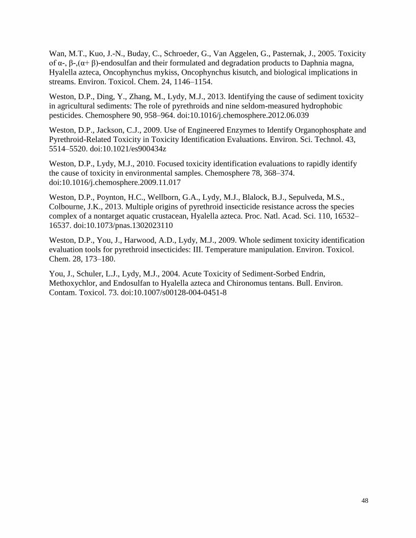
48
Wan, M.T., Kuo, J.-N., Buday, C., Schroeder, G., Van Aggelen, G., Pasternak, J., 2005. Toxicity
of α-, β-,(α+ β)-endosulfan and their formulated and degradation products to Daphnia magna,
Hyalella azteca, Oncophynchus mykiss, Oncophynchus kisutch, and biological implications in
streams. Environ. Toxicol. Chem. 24, 1146–1154.
Weston, D.P., Ding, Y., Zhang, M., Lydy, M.J., 2013. Identifying the cause of sediment toxicity
in agricultural sediments: The role of pyrethroids and nine seldom-measured hydrophobic
pesticides. Chemosphere 90, 958–964. doi:10.1016/j.chemosphere.2012.06.039
Weston, D.P., Jackson, C.J., 2009. Use of Engineered Enzymes to Identify Organophosphate and
Pyrethroid-Related Toxicity in Toxicity Identification Evaluations. Environ. Sci. Technol. 43,
5514–5520. doi:10.1021/es900434z
Weston, D.P., Lydy, M.J., 2010. Focused toxicity identification evaluations to rapidly identify
the cause of toxicity in environmental samples. Chemosphere 78, 368–374.
doi:10.1016/j.chemosphere.2009.11.017
Weston, D.P., Poynton, H.C., Wellborn, G.A., Lydy, M.J., Blalock, B.J., Sepulveda, M.S.,
Colbourne, J.K., 2013. Multiple origins of pyrethroid insecticide resistance across the species
complex of a nontarget aquatic crustacean, Hyalella azteca. Proc. Natl. Acad. Sci. 110, 16532–
16537. doi:10.1073/pnas.1302023110
Weston, D.P., You, J., Harwood, A.D., Lydy, M.J., 2009. Whole sediment toxicity identification
evaluation tools for pyrethroid insecticides: III. Temperature manipulation. Environ. Toxicol.
Chem. 28, 173–180.
You, J., Schuler, L.J., Lydy, M.J., 2004. Acute Toxicity of Sediment-Sorbed Endrin,
Methoxychlor, and Endosulfan to Hyalella azteca and Chironomus tentans. Bull. Environ.
Contam. Toxicol. 73. doi:10.1007/s00128-004-0451-8

49
(a)
(b)
Hyalella curvispina a
Hyalella azteca
Hyalella curvispina
0
0.1
0.2
0.3
0.4
0.5
0.6
0.7
0.8
0.9
1
0.01 0.10 1.00 10.00 100.00 1000.00 10000.00 100000.00
Porp
ort
ion o
f specie
s a
ffecte
d
Endosulfan LC50 (ug/L)
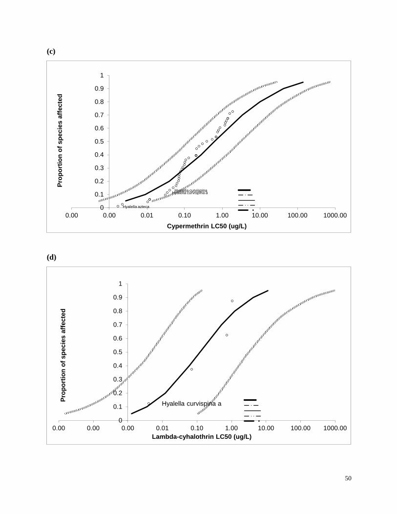
50
(c)
(d)
Hyalella curvispina aHyalella curvispina
Hyalella azteca0
0.1
0.2
0.3
0.4
0.5
0.6
0.7
0.8
0.9
1
0.00 0.00 0.01 0.10 1.00 10.00 100.00 1000.00
Pro
po
rtio
n o
f sp
ecie
s a
ffecte
d
Cypermethrin LC50 (ug/L)
Hyalella curvispina a
0
0.1
0.2
0.3
0.4
0.5
0.6
0.7
0.8
0.9
1
0.00 0.00 0.00 0.01 0.10 1.00 10.00 100.00 1000.00
Pro
po
rtio
n o
f sp
ecie
s a
ffecte
d
Lambda-cyhalothrin LC50 (ug/L)
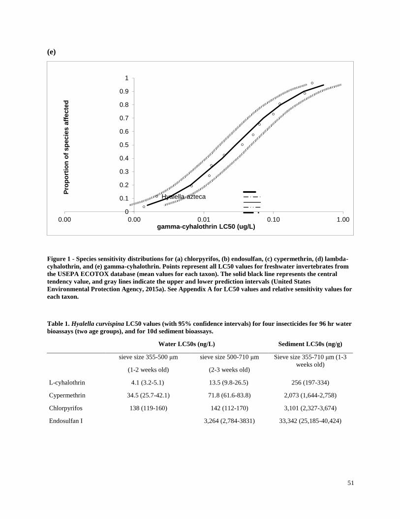
51
(e)
Figure 1 - Species sensitivity distributions for (a) chlorpyrifos, (b) endosulfan, (c) cypermethrin, (d) lambda-
cyhalothrin, and (e) gamma-cyhalothrin. Points represent all LC50 values for freshwater invertebrates from
the USEPA ECOTOX database (mean values for each taxon). The solid black line represents the central
tendency value, and gray lines indicate the upper and lower prediction intervals (United States
Environmental Protection Agency, 2015a). See Appendix A for LC50 values and relative sensitivity values for
each taxon.
Table 1. Hyalella curvispina LC50 values (with 95% confidence intervals) for four insecticides for 96 hr water
bioassays (two age groups), and for 10d sediment bioassays.
Water LC50s (ng/L) Sediment LC50s (ng/g)
sieve size 355-500 μm
(1-2 weeks old)
sieve size 500-710 μm
(2-3 weeks old)
Sieve size 355-710 μm (1-3
weeks old)
L-cyhalothrin 4.1 (3.2-5.1) 13.5 (9.8-26.5) 256 (197-334)
Cypermethrin 34.5 (25.7-42.1) 71.8 (61.6-83.8) 2,073 (1,644-2,758)
Chlorpyrifos 138 (119-160) 142 (112-170) 3,101 (2,327-3,674)
Endosulfan I 3,264 (2,784-3831) 33,342 (25,185-40,424)
Hyalella azteca
0
0.1
0.2
0.3
0.4
0.5
0.6
0.7
0.8
0.9
1
0.00 0.00 0.01 0.10 1.00
Pro
po
rtio
n o
f sp
ecie
s a
ffecte
d
gamma-cyhalothrin LC50 (ug/L)
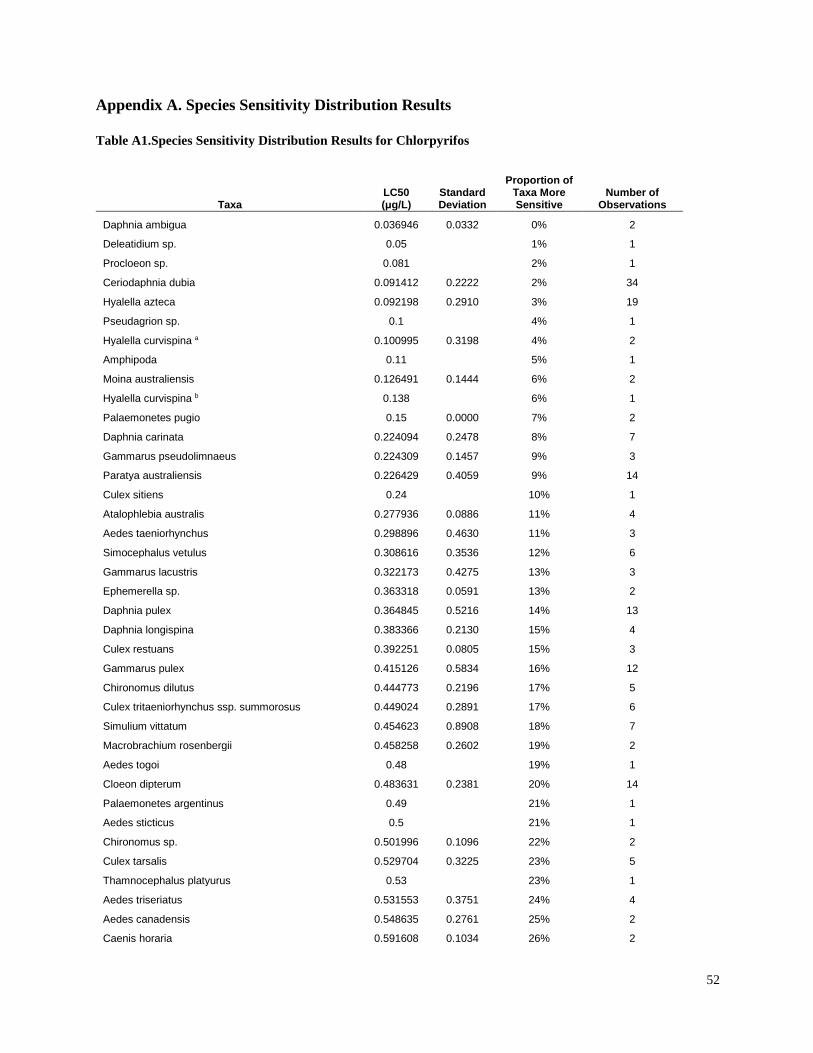
52
Appendix A. Species Sensitivity Distribution Results
Table A1.Species Sensitivity Distribution Results for Chlorpyrifos
Taxa LC50 (μg/L)
Standard Deviation
Proportion of Taxa More Sensitive
Number of Observations
Daphnia ambigua 0.036946 0.0332 0% 2
Deleatidium sp. 0.05 1% 1
Procloeon sp. 0.081 2% 1
Ceriodaphnia dubia 0.091412 0.2222 2% 34
Hyalella azteca 0.092198 0.2910 3% 19
Pseudagrion sp. 0.1 4% 1
Hyalella curvispina a 0.100995 0.3198 4% 2
Amphipoda 0.11 5% 1
Moina australiensis 0.126491 0.1444 6% 2
Hyalella curvispina b 0.138 6% 1
Palaemonetes pugio 0.15 0.0000 7% 2
Daphnia carinata 0.224094 0.2478 8% 7
Gammarus pseudolimnaeus 0.224309 0.1457 9% 3
Paratya australiensis 0.226429 0.4059 9% 14
Culex sitiens 0.24 10% 1
Atalophlebia australis 0.277936 0.0886 11% 4
Aedes taeniorhynchus 0.298896 0.4630 11% 3
Simocephalus vetulus 0.308616 0.3536 12% 6
Gammarus lacustris 0.322173 0.4275 13% 3
Ephemerella sp. 0.363318 0.0591 13% 2
Daphnia pulex 0.364845 0.5216 14% 13
Daphnia longispina 0.383366 0.2130 15% 4
Culex restuans 0.392251 0.0805 15% 3
Gammarus pulex 0.415126 0.5834 16% 12
Chironomus dilutus 0.444773 0.2196 17% 5
Culex tritaeniorhynchus ssp. summorosus 0.449024 0.2891 17% 6
Simulium vittatum 0.454623 0.8908 18% 7
Macrobrachium rosenbergii 0.458258 0.2602 19% 2
Aedes togoi 0.48 19% 1
Cloeon dipterum 0.483631 0.2381 20% 14
Palaemonetes argentinus 0.49 21% 1
Aedes sticticus 0.5 21% 1
Chironomus sp. 0.501996 0.1096 22% 2
Culex tarsalis 0.529704 0.3225 23% 5
Thamnocephalus platyurus 0.53 23% 1
Aedes triseriatus 0.531553 0.3751 24% 4
Aedes canadensis 0.548635 0.2761 25% 2
Caenis horaria 0.591608 0.1034 26% 2
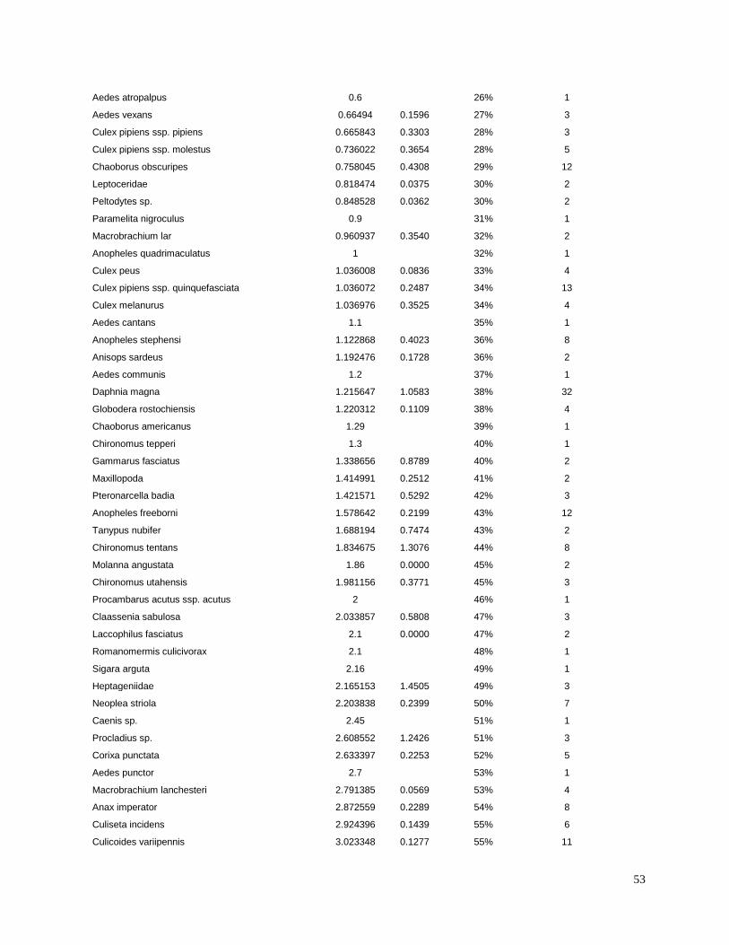
53
Aedes atropalpus 0.6 26% 1
Aedes vexans 0.66494 0.1596 27% 3
Culex pipiens ssp. pipiens 0.665843 0.3303 28% 3
Culex pipiens ssp. molestus 0.736022 0.3654 28% 5
Chaoborus obscuripes 0.758045 0.4308 29% 12
Leptoceridae 0.818474 0.0375 30% 2
Peltodytes sp. 0.848528 0.0362 30% 2
Paramelita nigroculus 0.9 31% 1
Macrobrachium lar 0.960937 0.3540 32% 2
Anopheles quadrimaculatus 1 32% 1
Culex peus 1.036008 0.0836 33% 4
Culex pipiens ssp. quinquefasciata 1.036072 0.2487 34% 13
Culex melanurus 1.036976 0.3525 34% 4
Aedes cantans 1.1 35% 1
Anopheles stephensi 1.122868 0.4023 36% 8
Anisops sardeus 1.192476 0.1728 36% 2
Aedes communis 1.2 37% 1
Daphnia magna 1.215647 1.0583 38% 32
Globodera rostochiensis 1.220312 0.1109 38% 4
Chaoborus americanus 1.29 39% 1
Chironomus tepperi 1.3 40% 1
Gammarus fasciatus 1.338656 0.8789 40% 2
Maxillopoda 1.414991 0.2512 41% 2
Pteronarcella badia 1.421571 0.5292 42% 3
Anopheles freeborni 1.578642 0.2199 43% 12
Tanypus nubifer 1.688194 0.7474 43% 2
Chironomus tentans 1.834675 1.3076 44% 8
Molanna angustata 1.86 0.0000 45% 2
Chironomus utahensis 1.981156 0.3771 45% 3
Procambarus acutus ssp. acutus 2 46% 1
Claassenia sabulosa 2.033857 0.5808 47% 3
Laccophilus fasciatus 2.1 0.0000 47% 2
Romanomermis culicivorax 2.1 48% 1
Sigara arguta 2.16 49% 1
Heptageniidae 2.165153 1.4505 49% 3
Neoplea striola 2.203838 0.2399 50% 7
Caenis sp. 2.45 51% 1
Procladius sp. 2.608552 1.2426 51% 3
Corixa punctata 2.633397 0.2253 52% 5
Aedes punctor 2.7 53% 1
Macrobrachium lanchesteri 2.791385 0.0569 53% 4
Anax imperator 2.872559 0.2289 54% 8
Culiseta incidens 2.924396 0.1439 55% 6
Culicoides variipennis 3.023348 0.1277 55% 11
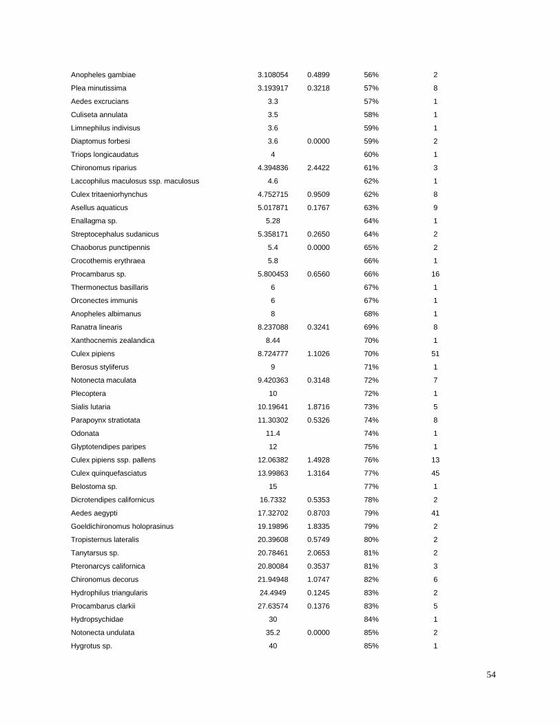
54
Anopheles gambiae 3.108054 0.4899 56% 2
Plea minutissima 3.193917 0.3218 57% 8
Aedes excrucians 3.3 57% 1
Culiseta annulata 3.5 58% 1
Limnephilus indivisus 3.6 59% 1
Diaptomus forbesi 3.6 0.0000 59% 2
Triops longicaudatus 4 60% 1
Chironomus riparius 4.394836 2.4422 61% 3
Laccophilus maculosus ssp. maculosus 4.6 62% 1
Culex tritaeniorhynchus 4.752715 0.9509 62% 8
Asellus aquaticus 5.017871 0.1767 63% 9
Enallagma sp. 5.28 64% 1
Streptocephalus sudanicus 5.358171 0.2650 64% 2
Chaoborus punctipennis 5.4 0.0000 65% 2
Crocothemis erythraea 5.8 66% 1
Procambarus sp. 5.800453 0.6560 66% 16
Thermonectus basillaris 6 67% 1
Orconectes immunis 6 67% 1
Anopheles albimanus 8 68% 1
Ranatra linearis 8.237088 0.3241 69% 8
Xanthocnemis zealandica 8.44 70% 1
Culex pipiens 8.724777 1.1026 70% 51
Berosus styliferus 9 71% 1
Notonecta maculata 9.420363 0.3148 72% 7
Plecoptera 10 72% 1
Sialis lutaria 10.19641 1.8716 73% 5
Parapoynx stratiotata 11.30302 0.5326 74% 8
Odonata 11.4 74% 1
Glyptotendipes paripes 12 75% 1
Culex pipiens ssp. pallens 12.06382 1.4928 76% 13
Culex quinquefasciatus 13.99863 1.3164 77% 45
Belostoma sp. 15 77% 1
Dicrotendipes californicus 16.7332 0.5353 78% 2
Aedes aegypti 17.32702 0.8703 79% 41
Goeldichironomus holoprasinus 19.19896 1.8335 79% 2
Tropisternus lateralis 20.39608 0.5749 80% 2
Tanytarsus sp. 20.78461 2.0653 81% 2
Pteronarcys californica 20.80084 0.3537 81% 3
Chironomus decorus 21.94948 1.0747 82% 6
Hydrophilus triangularis 24.4949 0.1245 83% 2
Procambarus clarkii 27.63574 0.1376 83% 5
Hydropsychidae 30 84% 1
Notonecta undulata 35.2 0.0000 85% 2
Hygrotus sp. 40 85% 1
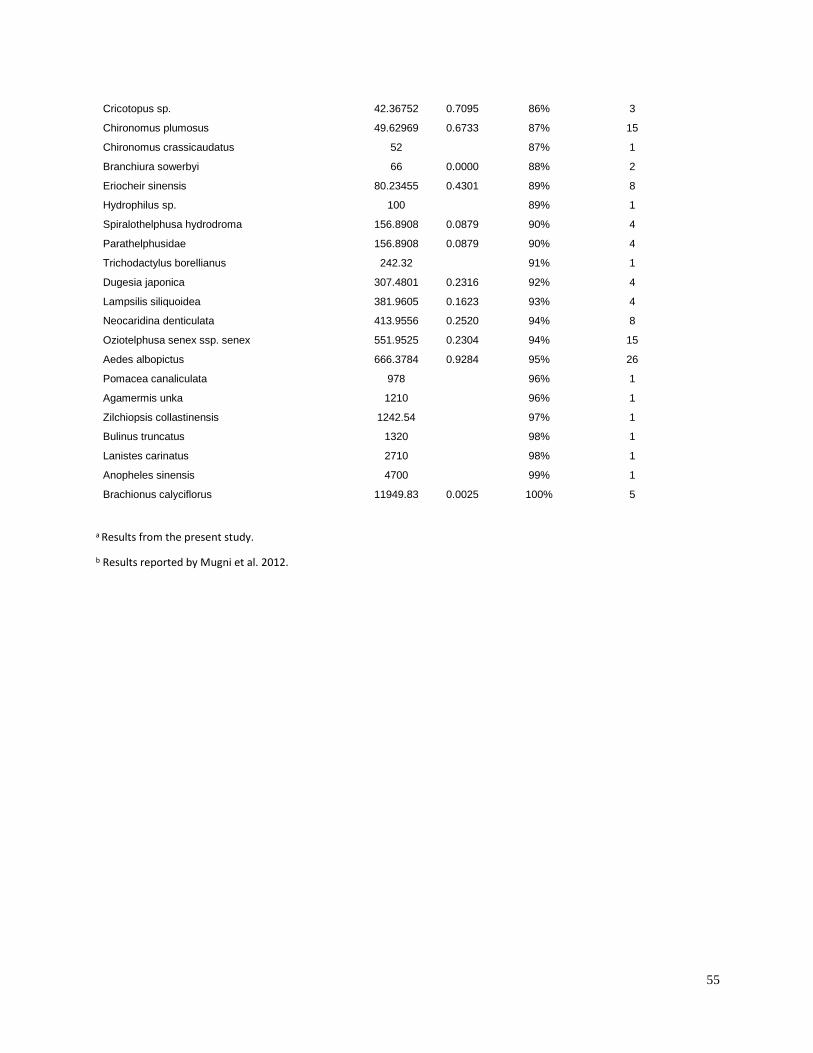
55
Cricotopus sp. 42.36752 0.7095 86% 3
Chironomus plumosus 49.62969 0.6733 87% 15
Chironomus crassicaudatus 52 87% 1
Branchiura sowerbyi 66 0.0000 88% 2
Eriocheir sinensis 80.23455 0.4301 89% 8
Hydrophilus sp. 100 89% 1
Spiralothelphusa hydrodroma 156.8908 0.0879 90% 4
Parathelphusidae 156.8908 0.0879 90% 4
Trichodactylus borellianus 242.32 91% 1
Dugesia japonica 307.4801 0.2316 92% 4
Lampsilis siliquoidea 381.9605 0.1623 93% 4
Neocaridina denticulata 413.9556 0.2520 94% 8
Oziotelphusa senex ssp. senex 551.9525 0.2304 94% 15
Aedes albopictus 666.3784 0.9284 95% 26
Pomacea canaliculata 978 96% 1
Agamermis unka 1210 96% 1
Zilchiopsis collastinensis 1242.54 97% 1
Bulinus truncatus 1320 98% 1
Lanistes carinatus 2710 98% 1
Anopheles sinensis 4700 99% 1
Brachionus calyciflorus 11949.83 0.0025 100% 5
a Results from the present study.
b Results reported by Mugni et al. 2012.

56
Table A2.Species Sensitivity Distribution Results for Endosulfan
Taxa LC50 (μg/L)
Standard Deviation
Proportion of Taxa More Sensitive
Number of Observations
Mesocyclops longisetus 0.017889 0.0686 1% 2
Eucyclops sp. 0.1 2% 1
Alonella sp. 0.2 3% 1
Paratelphusa jacquemontii 0.269189 0.2086 5% 4
Palaemonetes paludosus 0.337263 0.1232 6% 4
Daphnia longispina 0.34641 0.0884 8% 2
Diaptomus sp. 0.6 9% 1
Atalophlebia australis 0.62967 0.0786 10% 10
Cheumatopsyche sp. 0.69755 0.2589 12% 6
Paratya australiensis 0.699714 0.1943 13% 2
Cypria sp. 0.9 15% 1
Amphipoda 1 16% 1
Jappa kutera 1.429578 0.1879 17% 16
Cypris subglobosa 1.449138 0.2278 19% 2
Caridina laevis 1.558076 0.2602 20% 2
Hyalella curvispina a 3.2641 22% 1
Macrobrachium lamarrei 4.211157 0.0772 23% 4
Macrobrachium dayanum 5.042816 0.0754 24% 4
Macrobrachium rosenbergii 5.491317 0.8502 26% 8
Palaemonetes argentinus 6.28 27% 1
Gammarus lacustris 6.671231 0.0952 28% 4
Pteronarcys californica 6.761489 0.5142 30% 3
Gammarus fasciatus 7.113787 0.1281 31% 3
Hyalella azteca 7.285761 0.1718 33% 3
Asellus aquaticus 10 34% 1
Caridina weberi 12.7393 0.3529 35% 16
Atalophlebia sp. 13.59562 0.0482 37% 6
Eretes sticticus 15.81139 0.2814 38% 2
Moina micrura 16.2 40% 1
Sigara alternata 16.48171 0.1997 41% 3
Hyalella curvispinab 17.2 42% 1
Paramelita nigroculus 19.2 44% 1
Enallagma sp. 21.87933 0.1070 45% 3
Spicodiaptomus chelospinus 44.72136 0.0686 47% 2
Pseudagrion sp. 46 48% 1
Chironomus plumosus 53 49% 1
Radix luteola 60 51% 1
Culex pipiens ssp. quinquefasciata 66 52% 1
Culex quinquefasciatus 70.70557 2.8051 53% 4
Procambarus clarkii 100.7571 0.8812 55% 2
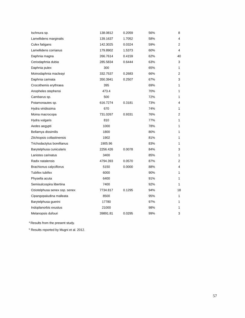
57
Ischnura sp. 138.0812 0.2059 56% 8
Lamellidens marginalis 139.1637 1.7052 58% 4
Culex fatigans 142.3025 0.0324 59% 2
Lamellidens corrianus 179.8902 1.5373 60% 4
Daphnia magna 266.7614 0.4159 62% 40
Ceriodaphnia dubia 285.5834 0.6444 63% 3
Daphnia pulex 300 65% 1
Moinodaphnia macleayi 332.7537 0.2683 66% 2
Daphnia carinata 350.3941 0.2507 67% 3
Crocothemis erythraea 395 69% 1
Anopheles stephensi 473.4 70% 1
Cambarus sp. 500 72% 1
Potamonautes sp. 616.7274 0.3181 73% 4
Hydra viridissima 670 74% 1
Moina macrocopa 731.0267 0.9331 76% 2
Hydra vulgaris 810 77% 1
Aedes aegypti 1000 78% 1
Bellamya dissimilis 1800 80% 1
Zilchiopsis collastinensis 1902 81% 1
Trichodactylus borellianus 1905.96 83% 1
Barytelphusa cunicularis 2256.426 0.0078 84% 3
Lanistes carinatus 3400 85% 1
Radix natalensis 4794.393 0.0570 87% 2
Brachionus calyciflorus 5150 0.0000 88% 4
Tubifex tubifex 6000 90% 1
Physella acuta 6400 91% 1
Semisulcospira libertina 7400 92% 1
Oziotelphusa senex ssp. senex 7734.817 0.1295 94% 18
Cipangopaludina malleata 8500 95% 1
Barytelphusa guerini 17780 97% 1
Indoplanorbis exustus 21000 98% 1
Melanopsis dufouri 39891.81 0.0295 99% 3
a Results from the present study.
b Results reported by Mugni et al. 2012.
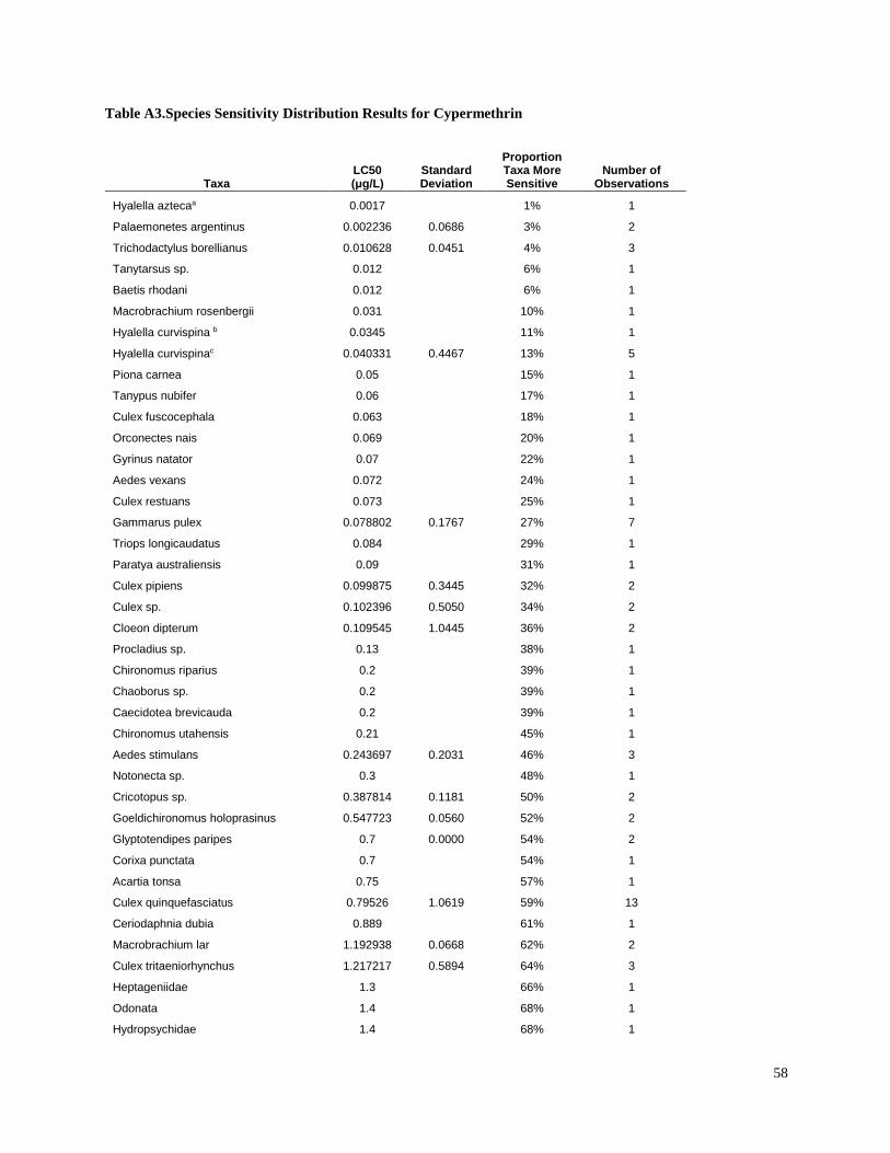
58
Table A3.Species Sensitivity Distribution Results for Cypermethrin
Taxa LC50 (μg/L)
Standard Deviation
Proportion Taxa More Sensitive
Number of Observations
Hyalella aztecaa 0.0017 1% 1
Palaemonetes argentinus 0.002236 0.0686 3% 2
Trichodactylus borellianus 0.010628 0.0451 4% 3
Tanytarsus sp. 0.012 6% 1
Baetis rhodani 0.012 6% 1
Macrobrachium rosenbergii 0.031 10% 1
Hyalella curvispina b 0.0345 11% 1
Hyalella curvispinac 0.040331 0.4467 13% 5
Piona carnea 0.05 15% 1
Tanypus nubifer 0.06 17% 1
Culex fuscocephala 0.063 18% 1
Orconectes nais 0.069 20% 1
Gyrinus natator 0.07 22% 1
Aedes vexans 0.072 24% 1
Culex restuans 0.073 25% 1
Gammarus pulex 0.078802 0.1767 27% 7
Triops longicaudatus 0.084 29% 1
Paratya australiensis 0.09 31% 1
Culex pipiens 0.099875 0.3445 32% 2
Culex sp. 0.102396 0.5050 34% 2
Cloeon dipterum 0.109545 1.0445 36% 2
Procladius sp. 0.13 38% 1
Chironomus riparius 0.2 39% 1
Chaoborus sp. 0.2 39% 1
Caecidotea brevicauda 0.2 39% 1
Chironomus utahensis 0.21 45% 1
Aedes stimulans 0.243697 0.2031 46% 3
Notonecta sp. 0.3 48% 1
Cricotopus sp. 0.387814 0.1181 50% 2
Goeldichironomus holoprasinus 0.547723 0.0560 52% 2
Glyptotendipes paripes 0.7 0.0000 54% 2
Corixa punctata 0.7 54% 1
Acartia tonsa 0.75 57% 1
Culex quinquefasciatus 0.79526 1.0619 59% 13
Ceriodaphnia dubia 0.889 61% 1
Macrobrachium lar 1.192938 0.0668 62% 2
Culex tritaeniorhynchus 1.217217 0.5894 64% 3
Heptageniidae 1.3 66% 1
Odonata 1.4 68% 1
Hydropsychidae 1.4 68% 1
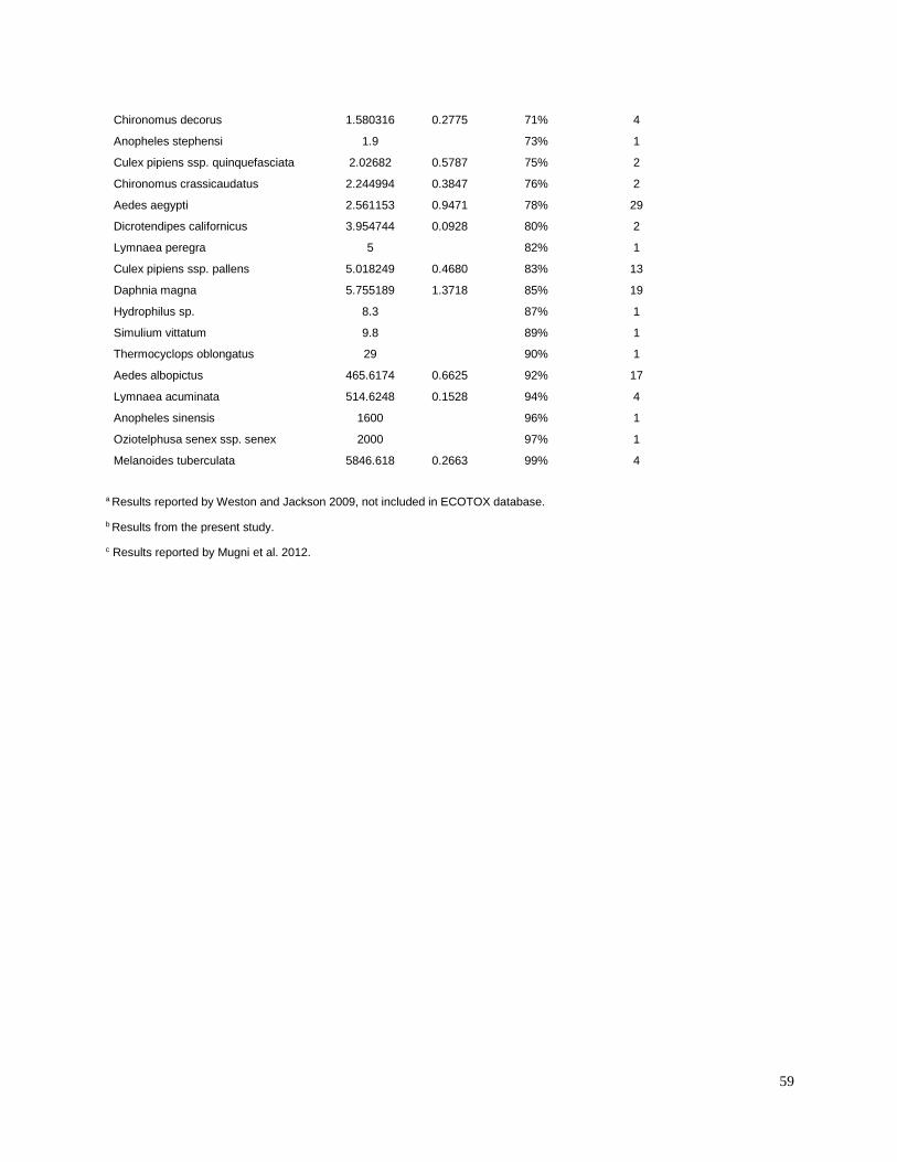
59
Chironomus decorus 1.580316 0.2775 71% 4
Anopheles stephensi 1.9 73% 1
Culex pipiens ssp. quinquefasciata 2.02682 0.5787 75% 2
Chironomus crassicaudatus 2.244994 0.3847 76% 2
Aedes aegypti 2.561153 0.9471 78% 29
Dicrotendipes californicus 3.954744 0.0928 80% 2
Lymnaea peregra 5 82% 1
Culex pipiens ssp. pallens 5.018249 0.4680 83% 13
Daphnia magna 5.755189 1.3718 85% 19
Hydrophilus sp. 8.3 87% 1
Simulium vittatum 9.8 89% 1
Thermocyclops oblongatus 29 90% 1
Aedes albopictus 465.6174 0.6625 92% 17
Lymnaea acuminata 514.6248 0.1528 94% 4
Anopheles sinensis 1600 96% 1
Oziotelphusa senex ssp. senex 2000 97% 1
Melanoides tuberculata 5846.618 0.2663 99% 4
a Results reported by Weston and Jackson 2009, not included in ECOTOX database.
b Results from the present study.
c Results reported by Mugni et al. 2012.
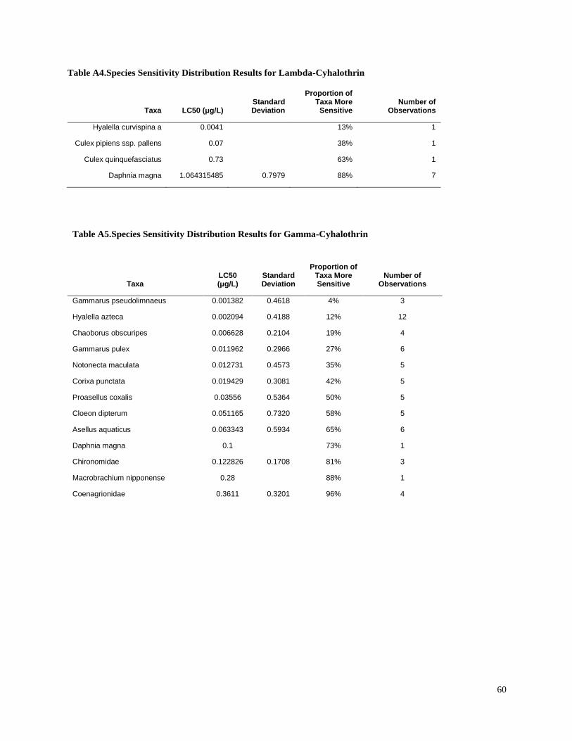
60
Table A4.Species Sensitivity Distribution Results for Lambda-Cyhalothrin
Taxa LC50 (μg/L) Standard Deviation
Proportion of Taxa More Sensitive
Number of Observations
Hyalella curvispina a 0.0041 13% 1
Culex pipiens ssp. pallens 0.07 38% 1
Culex quinquefasciatus 0.73 63% 1
Daphnia magna 1.064315485 0.7979 88% 7
Table A5.Species Sensitivity Distribution Results for Gamma-Cyhalothrin
Taxa LC50 (μg/L)
Standard Deviation
Proportion of Taxa More Sensitive
Number of Observations
Gammarus pseudolimnaeus 0.001382 0.4618 4% 3
Hyalella azteca 0.002094 0.4188 12% 12
Chaoborus obscuripes 0.006628 0.2104 19% 4
Gammarus pulex 0.011962 0.2966 27% 6
Notonecta maculata 0.012731 0.4573 35% 5
Corixa punctata 0.019429 0.3081 42% 5
Proasellus coxalis 0.03556 0.5364 50% 5
Cloeon dipterum 0.051165 0.7320 58% 5
Asellus aquaticus 0.063343 0.5934 65% 6
Daphnia magna 0.1 73% 1
Chironomidae 0.122826 0.1708 81% 3
Macrobrachium nipponense 0.28 88% 1
Coenagrionidae 0.3611 0.3201 96% 4
61
CHAPTER 4
Effects of insecticides on stream invertebrate communities in soy production regions of the
Argentine Pampas
62
Effects of insecticides on stream invertebrate communities in soy production regions of the
Argentine Pampas
Abstract
We investigated relationships among insecticides and aquatic invertebrate communities in 22
streams of two soy production regions of the Argentine Pampas over three growing seasons.
Chlorpyrifos, endosulfan, cypermethrin and lambda-cyhalothrin were the insecticides most
frequently detected in stream sediments. The Species at Risk (SPEAR) pesticide bioassessment
index (SPEARpesticides)was applied to evaluate relationships between sediment insecticide toxic
units (TUs) and invertebrate communities associated with both benthic habitats and emergent
vegetation. The SPEAR trait thresholds for classification of taxa with respect to generation time
and pesticide sensitivity were optimized for the Argentina data sets. SPEARpesticides was the only
response metric that was significantly correlated with total insecticide TU values for all three
averaged data sets, consistently showing a trend of decreasing values with increasing TU values
(r2 = 0.35 to 0.42, p-value = 0.001 to 0.03). Although pyrethroids were the insecticides that
contributed the higest TU values, toxicity calculated based on all insecticides was better at
predicting changes in invertebrate communities than toxicity of pyrethroids alone. Crustaceans,
particularly the amphipod Hyalella spp., which are relatively sensitive to pesticides, played a
large role in the performance of SPEARpesticides, and the relative abundance of all crustaceans also
showed a significant decreasing trend with increasing insecticide TUs for two of three data sets
(r2 = 0.30 to 0.57, p-value = 0.003 to 0.04). For all data sets, total insecticide TU was the most
important variable in explaining variance in the SPEARpesticide index. This study was the first
application of the SPEAR index in South America, and the first oneto use it to evaluate effects of
pesticides on invertebrate communities associated with aquatic vegetation. Although the SPEAR
index was developed in Europe, it performed well in the Argentine Pampas with only minor
modifications, andwould likely improve in performance as more data are obtained on South
American taxa traits, such as pesticide sensitivity and generation time.
Introduction
The Argentine Pampas is the central plain of Argentina with a mild climate and very fertile soil.
Previously covered by grasslands, it is now the most productive agricultural region of the
country. Over the last three decades, soybeans have become a major export crop for Argentina,
and increased pesticide use has led to concerns about environmental effects. For example,
between 1995 and 2011, soy cultivation area expanded by 209% in Argentina (Castanheira and
Freire, 2013). Most global soy production occurs in North and South America, although a large
part of the soy is exported to Europe and China, primarily for use as animal feed (Garrett et al.,
2013). Pesticide consumption in Argentina increased from 6 million kilograms in 1992 (Pengue,
2000) to 32 million kilograms in 2012 (CASAFE, 2013). Insecticide application rates are
approximately double those of fungicides, and the insecticides most frequently used in soy
production (pyrethroids, chlorpyrifos, and endosulfan) have very high aquatic toxicity (Hunt et
al., 2016; Nordborg et al., 2014).
Multiple studies have detected soy production insecticides in both sediment and water collected
from streams in Argentina (Di Marzio et al., 2010; Hunt et al., 2016; Jergentz et al., 2005;
Marino and Ronco, 2005; Mugni et al., 2011), but there is a lack of field studies investigating
63
effects to aquatic invertebrate communities. Several studies in Argentina have found associations
between stream insecticide concentrations and effects on the native amphipod Hyalella
curvispina using single-species toxicity tests (Di Marzio et al., 2010; Jergentz et al., 2004a;
Mugni et al., 2011). Also, Jergentz et al. (2004b) found that a pulse of endosulfan was associated
with reductions in abundances of Odonata and Ephemeroptera in two small Pampas streams).
However, to date no study in the region has documented widespread insecticide effects on
aquatic invertebrate communities.
The Species at Risk pesticide index (SPEARpesticides) was developed in Europe to evaluate effects
of pesticides on benthic macroinvertebrate communities (Liess and Von der Ohe, 2005), and has
been applied successfully in several continents (Schäfer et al., 2012). For example, significant
correlations have been found between the SPEARpesticides index and pesticide concentrations in
streams in 8 countries in Europe, as well as in Australia and Siberia (r2 between 0.62 and 0.68)
(Schäfer et al., 2012). The SPEARpesticides index has been shown to respond selectively to
pesticide stressors and to be relatively insensitive to most other stressors, although its
performance can be affected by severe habitat degradation (siltation and channelization) and low
dissolved oxygen (Liess et al., 2008a; Jes Jessen Rasmussen et al., 2011; Schäfer et al., 2011,
2007).
The objectives of the present study were to: (1) evaluate relationships between insecticide
concentrations in stream sediments and aquatic invertebrate communities of the Argentine
Pampas using the SPEAR index; (2) examine the major changes in invertebrate communities
associated with pesticide exposure; and (3) test the applicability of the SPEAR index to
invertebrate communities associated with both benthos and emergent vegetation.
Methods and Materials
Study Locations and Sampling Schedule
We carried out the study over a three year period (Dec 2011 – Feb 2014), monitoring 23 sites in
small streams located in two regions of the Argentine Pampas, including an intensive soy
production region and a mixed agriculture and livestock region (Figure 1; Table S1). In the La
Plata region, the principal land use was cattle grazing, with scattered plots of soy production and
other agriculture. In the Arrecifes region, intensive soy production was the predominant land use.
In the La Plata region, four streams were sampled during two monitoring events in the 2011 to
2012 season only, including four sampling sites in one watershed and the remaining sites in
separate watersheds. In the Arrecifes region, 16 sites were sampled over three years (2012-2014),
and all sampling sites were on tributaries of the Arrecifes River.
Catchments were delineated using topographical maps to estimate catchment size (Table S2).
Substrates in streams of both regions generally consisted of sediment with no rocks and little
woody debris, although a few sites in Arrecifes contained some gravel. Stream depths ranged
from about 0.6 m to > 2 m (although all except two in the La Plata region were < 1 m), and
widths ranged from about 3 m to about 25 m (Table S2). Most streams included emergent (e.g.
Typha spp. and Scirpus spp.) and submerged vegetation (e.g. Potamogeton, Ceratophyllum and
Egeria), and many in the La Plata region were also characterized by abundant floating vegetation
(e.g. Eichornia, Lemna and Azolla).

64
Biological, physico-chemical, and insecticide concentration components involved concurrent
stream sampling that was generally timed to occur within a week after a heavy rainfall during or
soon after the peak insecticide application period, which usually occurs between December and
March. During the 2011-2012 growing season, samples in the La Plata region were collected in
December 2011 and March 2012, and in the Arrecifes region in January and March 2012. During
2013 and 2014, samples were collected only in Arrecifes, in February of both years (Table 1).
Physico-chemico, habitat and geographical variables
At each sampling site, pH, conductivity, dissolved oxygen, and temperature were measured with
a Yellow Springs Instruments SI 556 multi-parameter probe (Yellow Springs, OH, USA). During
2013 – 2014, turbidity was measured with a portable turbidity meter (Hanna Instruments 93414,
Woonsocket, RI, USA). Sediment samples were collected for sediment grain size analysis, and
organic carbon analysis by ferrous sulfate titration (USDA 1996) (Table S2).
Water samples for analysis of nutrients and major ions were collected in 1 l bottles and kept in
coolers with ice until analyzing or freezing within 24 hours of collection. Water samples were
filtered (Whatman GF/C) and suspended solids were measured based on weight of filtered
material. Dissolved nutrient and major ion concentrations were determined in the filtered water
(APHA 2005). Soluble reactive phosphorus was determined by colorimetry through reaction with
molybdate-ascorbic acid; nitrite and nitrate by hydrazine reduction followed by diazotization;
and ammonium by the reaction of indophenol blue (APHA 2005). Calcium and magnesium were
determined by atomic absorption, sodium and potassium by photometry, bicarbonates by Gran
titration, sulfates by turbidimetry, and chlorides by silver nitrate titration (APHA 2005).
At each site visit, maximum stream width and depth were measured. Catchments for each site
were delineated in GIS using topographical layers, and catchment areas were calculated.
Elevation and stream gradient immediately upstream of each site was estimated based on
topographical contours (Table S2). In 2013 – 2014, stream velocity was measured and
approximate percent area coverage of emergent, submerged, and floating vegetation was
estimated (Table S2).
Sediment sample collection and insecticide analysis
The methods for sediment sample collection and analysis of insecticides have been previously
described (Hunt et al., 2016). Briefly, composite sediment samples were prepared from 3 to 5
locations at each site, and insecticides were extracted from sediments by sonication (You et al.
2008). Samples collected in 2011-2012 were analyzed for cypermethrin, lambda-cyahalothrin,
endosulfan and chloryrifos by gas chromatography-electron capture detection (GC-ECD).
Samples collected in 2013-2014 were analyzed for the same insecticides plus additional
pyrethroid and organochlorine insecticides using gas chromatography – mass spectrometry –
negative chemical ionization (GC-MS-NCI).
Toxic unit calculation
Insecticide toxic units (TUs) were calculated for all sediment samples:
TU = Ci /EC50i
65
where Ci was the insecticide concentration in sediment normalized for total organic carbon
(TOC), and EC50iwas the 10-d median effects concentration for mortality or immobilization for
each insecticide.
The sediment LC50 values for freshwater aquatic invertebrates were identified for sensitive
species (Table 2). Most of the LC50 values used in the present study were for the amphipod
Hyalella azteca, which is known to be very sensitive to pyrethroids and chlorpyrifos (Weston and
Lydy 2010). Although H. azteca does not occur in Argentina, several closely related species (H.
curvispina, H. pampeana, and H. pseudoazteca) are important components of the aquatic
invertebrate communities in the Pampas, and the pesticide sensitivity of H. curvispina has been
shown to be similar to that of H. azteca (Mugni et al., 2013; Hunt, unpublished data). For
endosulfan, Chironomus tentans was more sensitive than H. azteca (You et al., 2004);
accordingly, the LC50 for C. tentans was used to calculate the TU. Toxicity of pesticides in
sediment is highly dependent on organic carbon content; therefore, the concentrations were
normalized for total organic carbon to calculate TU values.
TU values for all insecticides were summed to calculate total insecticide TUs, and TU values for
all pyrethroid insecticides were used to calculate total pyrethroid TUs. When summing TU
values, all insecticides that were detected in the data set were included, assigning a concentration
of half the quantification limit for pesticides that were not detected in the sample, or detected
below the reporting limit. This approach was used because many of the insecticides were
frequently detected below the reporting limit; thus it was known that they were present but could
not be accurately quantified (Hunt et al., 2016). The data sets for each sampling event were not
an adequate size to use a statistical approach such as maximum likelihood estimate to estimate
values of concentrations below the quantification limit (Helsel, 2012). While this approach may
overestimate total TU values in some samples, in most cases the insecticides not detected in a
sample did not contribute more than 1% of the total TU value. Insecticides that were measured
but not detected in the relevant sample group were not included in TU calculations for that
sample group.
Macroinvertebrate collection and identification
Benthic macroinvertebrate samples were collected by dragging a 30cm D-frame dip net with 500
µm mesh (Wildco, Yulee, FL, USA) over the bottom sediment of each 1 m transect. Because of
high variability in the number of organisms obtained, sample size was adapted over time to
ensure a sufficient number of organisms in each sample (Table 1). In 2011-2013, all invertebrates
from the entire composite sample (approximately 1.5m2 in 2011-2012, 2.7m2 in 2013) were
sorted and identified. In 2014, a subsampling method was used. A sample of approximately 2.7
m2 was obtained at each site, and the sample material was homogenized and divided into 24
quadrats. Organisms from randomly selected quadrats were sorted until a total count of 500
organisms per sample was reached, or until organisms from all quadrats were sorted. This is
close to the upper range of counts used in US biomonitoring programs involving fixed-numbers
of organisms (Carter and Resh, 2013). Once initiating the sorting of a quadrat, it was finished to
completion even if the target of 500 organisms was reached before finishing the quadrat.
Macroinvertebrate communities associated with emergent vegetation were sampled only during
2011-2012, and only at sites with sufficient emergent vegetation. Five 1m vegetation transects
66
were swept with a 30cm D-frame dip net (net opening area of approximately 600 cm2) with 500
µm mesh (Wildco, Yulee, FL, USA), for a total sample area of approximately 1.5m2.
All samples were preserved in the field in 80% ethanol, later sieved (500 µm) in the laboratory,
sorted under 3X magnification, and identified under a stereoscopic microscope. Insects, hydroids,
decapods, and amphipods were generally identified to family or lower level, and other taxa were
identified by higher taxonomic groups (oligochaetes, nemerteans, turbellarians, leeches,
nematodes, gastropods, bivalves, isopods, ostracods) using keys from Dominguez and Fernandez
(2009) and Merritt and Cummins (2008).
SPEAR index and optimization of sensitivity thresholds
The SPEARpesticides index classifies each taxon as either ‘‘species at risk’’ or ‘‘species not at
risk’’ based on four biological traits: (1) physiological sensitivity to organics compounds (2)
generation time; (3) pesticide exposure potential; and (4) migration ability (Liess and Ohe, 2005).
In the current version of the SPEARpesticides index (http://www.systemecology.eu/spearcalc/,
Version 0.9.0), binary values are assigned for each trait as follows: (1) physiological sensitivity
of 1 for taxa with relative sensitivity > threshold, otherwise 0; (2) generation time sensitivity of 1
for taxa with generation time > = threshold, otherwise 0; (3) exposure sensitivity of 1 for
epibenthic taxa, or 0 for sediment-dwelling taxa; and (4) migration sensitivity of 0 for organisms
with documented ability to migrate rapidly, 1 for all others. A taxon is defined as ‘‘species at
risk’’ only if values for all four traits are equal to 1.
The SPEARpesticides value for each sample is defined as:
where n is the number of taxa, xi is the abundance of the taxon i and y is 1 if taxon i is classified
as “species at risk”, otherwise 0.
Although in the present study some taxa were identified to genus or species level in some
samples, they could not consistently be identified to a level lower than family; therefore we used
family as the lowest taxonomic level for calculation of SPEARpesticides values. Some families
found in the present study were not included in the existing SPEAR database, which was based
primarily on European taxa; for these missing families we assigned the trait values available for
higher taxonomic levels.
It is likely that generation times of similar multivoltine taxa in the Pampas are shorter than in
most temperate zones because they can reproduce during most of the year. Although
reproduction of some taxa in Pampas streams may be greatly reduced during some periods of the
year,sufficient data do not exist to identify generation times of local taxa. In addition, the
invertebrate community composition of Pampas streams may be different than communities in
the temperate streams where the SPEARpesticides index has been validated. For SPEARpesticides, the
67
default threshold value for physiological sensitivity to pesticides is -0.36 (a taxon must have a
relative sensitivity score greater than -0.36 to be considered sensitive). The relative sensitivity
score for each taxon is calculated relative to Daphnia magna (Von der Ohe and Liess, 2004). The
default threshold value for generation time is 0.5 yr (a taxon must have a generation time of at
least 0.5 yr to be considered sensitive). These threshold values can be adjusted based on local
invertebrate communities. In the present study, we used an optimization approach to adjust the
pesticide sensitivity and generation time thresholds using Argentine Pampas data sets.
For each data group A to E (Table 1), we simultaneously optimized the values for the pesticide
sensitivity and generation time thresholds to achieve maximum inverse correlation between
SPEAR values and log-transformed TU values. Global optimization was performed with the
differential evolution algorithm, using the DEoptim package in R (Mullen et al., 2011). To avoid
overfitting to data sets with small sample size, optimum threshold values calculated for each of
the four benthic invertebrate sample groups (A-D) were averaged to obtain final threshold values
applied to all benthic and vegetation-associated invertebrate samples. It is reasonable to expect
that the optimum threshold values may be different for vegetation-associated communities than
for benthic communities, but there were two few vegetation-associated invertebrate samples to
perform optimization without high potential for overfitting.
The default SPEAR exposure potential values are based on exposure in the water column
because the SPEARpesticides index has mostly been related to pesticide concentrations in water.
However, insecticides in the present study were measured in sediment, because these insecticides
are hydrophobic and more likely to be adsorbed to sediments than to be dissolved in water.
Therefore, insecticide exposure to both epibenthic and sediment dwelling organisms is likely to
be high. Consequently, as part of the SPEARpesticides optimization process, we compared the
results using default taxa exposure values, and exposure values of 1 (exposed) for all epibenthic
and sediment-dwelling taxa.
Additional bioassessment metrics
In addition to the SPEARpesticides index, we calculated the relative abundance metrics of taxa
groups that were selected based on their high abundance in the region, and/or known high
sensitivity or tolerance to pesticides and other pollutants (Table 3) (Chang et al., 2014; Rubach et
al., 2010). We also calculated the Shannon diversity index and taxa richness. Samples containing
more than 300 organisms were rarefied to a constant size of 300 organisms to reduce the effect of
sample size (Barbour and Gerritsen, 1996).
Data analysis
We performed regression analysis on three data sets, each of which contained variable values that
were averaged over two sampling events (Table 1). For benthic invertebrate samples, we used
average values for the two events in 2011-2012, and for the two events in 2013-2014. For
vegetation-associated invertebrate samples, we used average values for the two events in 2011-
2012.
68
First, we calculated univariate linear regression relationships (lm function in R version 3.2.2)
between insecticide TU values (log transformed) and all response metrics (Table 3). For metrics
that were significantly correlated with log TU values, we then performed multiple linear
regression to evaluate the relative importance of insecticides and other variables in determining
variance in each response metric.
At each site we had measured values for many water quality, habitat, and watershed
characteristics (Table S2), many of which were highly correlated. To avoid predictor variables
with high collinearity, we used a correlation matrix to select variables that were highly correlated
with response variables but not with other predictor variables. After initial variable selection, we
checked variance inflation factors (VIFs) with the full model to avoid high collinearity (“vif”
function in R package “cor”) to confirm that all VIFs for all variables were < 3.
We then selected the best predictive models based on Akaike information criterion values
corrected for small sample size (AICc) and p-values. The ΔAICc for each model was calculated
as the difference between the AICc for the model and the lowest AICc of all models. For each
predictor variable in selected models with ΔAICc < 4 and p-value < 0.05, we determined the
magnitude and direction of coefficients using multi-model averaging across selected models
(Grueber et al., 2011) using the dredge and model.avg functions in the R package MuMIn
version 1.15.1 (Barton, 2015). Relative importance of each predictor variable was calculated as
the relativized sum of the Akaike weights over all of the selected models containing the variable
of interest (Barton, 2015). Importance ranges from 0 (parameter not given any explanatory
weight in any of the selected model) to 1 (parameter included in all selected models).
Results
Insecticide TU values
The most commonly detected insecticides were also those that are reported to be the most heavily
used in soy production in Argentina: chlorpyrifos, endosulfan (and its degradation product
endosulfan sulfate), cypermethrin, and lambda-cyhalothrin (Table 2). Bifenthrin and
organochlorine insecticides were detected only occasionally.
Insecticide detection patterns varied between the two regions. In the mixed agriculture region of
La Plata, the maximum total insecticide TU values for the 2011 and 2012 sampling events were
0.66 and 0.14 (based on C. tentans&H. azteca), and chlorpyrifos was the only insecticide that
was consistently detected. In the intensive soy production region of Arrecifes, maximum total
insecticide TU values for the four sampling events ranged from 0.51 to 1.36, and multiple
insecticides were detected at most locations (Table 2). In Arrecifes, pyrethroid (cypermethrin and
lambda-cyhalothrin) concentrations were the primary contributors to high TU values, while in La
Plata endosulfan was the primary contributor.
69
SPEARpesticides threshold optimization
Based on optimization results, we selected SPEARpesticides trait sensitivity threshold values to use
for the regression analysis. The pesticide sensitivity threshold was optimized at a range between -
0.24 and 0.06, and we selected a value of -0.2. The generation time threshold was optimized at a
range between 0 and 0.5 year, and we selected a value of 0.5 because this is the threshold value
that has been applied in other SPEARpesticides studies. Applying these threshold values, the only
taxa that were considered sensitive with respect to all four traits (overall SPEARpesticides score of
one) were the Trichoptera family Hydroptilidae, and all Crustacea taxa (Hyalellidae,
Palaemonidae, Aeglidae, Caridae, Ostracoda). For most data sets, slightly better correlations
were achieved when exposure values for all taxa (both epibenthic and sediment dwelling) were
set equal to 1 (sensitive with respect to exposure), so we set exposure values equal to 1 for all
taxa.
Univariate linear regressions
SPEARpesticideswas the metric that performed most consistently well in predicting invertebrate
community response to insecticides. SPEARpesticides, % crustaceans and % amphipods were the
only response metrics that were significantly correlated with insecticide TUs for more than one
data group (Table 3). The only other community metric that exhibited a significant correlation
with TU was % bivalvia, which was inversely correlated with pyrethroid TU only for the 2013-
2014 benthos data group. SPEARpesticides was the only response metric that was significantly
correlated with total insecticide TU values for all three averaged data sets, consistently showing a
trend of decreasing values with increasing TU values (r2 = 0.35 to 0.42, p-value = 0.001 to 0.03)
(Table 3; Figure 2). Percent crustaceans and % amphipods were significantly correlated with
total insecticide TU values in two of the three data groups. The relative abundance of both
crustaceans and amphipods were highly correlated for all data sets (0.39 < r2< 0.98; p-value
<0.018), and the two metrics performed very similarly (Table 3).
Total insecticide TU was usually a better predictor than pyrethroid TU for the three most
responsive metrics (SPEARpesticides, % crustaceans, and % amphipods), with the exception of the
2013-2014 benthos data group. Although significant correlations were obtained between
pyrethroid TU and some predictor variables (SPEARpesticides, % crustaceans and % amphipods),
the correlations were weaker than those for total insecticide TU.
Relative importance of variables
Based on univariate results, two response metrics (SPEARpesticidesand % crustacea) were selected
for multivariate linear regression to determine the relative importance of insecticide TU and non-
pesticide parameters. Amphipods were not included in this analysis because their response is
very similar to that of total crustacea (Table 3).
For all data sets, total insecticide TU was the most important variable in explaining variance in
the SPEARpesticides index (Table 4). The relative variable importance of total insecticide TU

70
ranged from 0.85 to 1.00 for the three data groups. Relative importance of non-pesticide
predictor variables used in models that included total insecticide TU ranged from 0.10 to 0.38.
Chloride was found to be important in explaining variability in relative abundance of
crustaceans, but less so for SPEARpesticides. Major ions were measured only in 2011-2012, and
many of the eight major ions were found to be collinear with each other, with conductivity, and
with TU values. To avoid redundancy, chloride was the only ion selected as a predictor variable
in the full models for 2011-2012, because it had low negative correlation with TUs and high
correlation with two response metrics (SPEARpesticides and % crustacea). For the 2013-2014 data
set, conductivity was selected instead of chloride, because major ions were not measured.
Chloride was identified as a variable with low to high importance in most of the 2011-2012
averaged models (Table 4). In particular, it had high importance in explaining the variance in %
crustacea (relative importance 0.57-1.00). Total conductivity was not found to be important in
explaining variance of any response metrics for the 2013-2014 data set. For 2011-2012, the
models were also run using conductivity in place of chloride to compare their relative
importance, and the importance of conductivity was consistently lower than chloride (not
shown).
Nutrients did have some influence on the SPEARpesticides index, but no apparent influence on the
relative abundance of crustaceans. Nutrient concentrations were measured during all sampling
events, and some nutrients were collinear. Most were also positively correlated with TU values,
but not with response metrics. Soluble reactive phosporous (SRP) was selected as a predictor
variable in the full models, because it had low correlation with TUs. SRP was identified as a
variable with low to moderate importance in the SPEARpesticides models, but had no importance in
explaining variance in % crustacea (Table 4).
Streams size did not appear to influence the SPEARpesticides index values, but was more important
in explaining variability in crustacean abundance. Several metrics were available to represent
stream size, including width, depth, elevation, gradient, and catchment area. Depth was selected
as a predictor variable in the full models, because it was the stream size variable with lowest
correlation with TUs. Depth was identified as an important variable for only one data set (2011-
2012 benthos), where it had high importance in explaining % crustacea (Table 4).
Floating vegetation % was the type of vegetation most highly correlated with response metrics,
and was included in the full model for 2013-2014 but was not found to be an important predictor
for any metric. Vegetation was not included in the 2011-2012 models because no quantitative
data were collected.
Discussion
The results of the present study demonstrate that insecticide concentrations in streams of the
Argentina Pampas are correlated with changes to aquatic invertebrate community compositions,
and that these changes are not highly influenced by other variables included in the study. To our
knowledge, this is the first field study that has demonstrated such effects in soy production
regions. In intensive soy production regionsinthe midwest region of the United States, as well as
in Brazil and Argentina, many studies have reported frequent detections of insecticides, as well
as toxicity to specific sensitive species (Casara et al., 2012; Di Marzio et al., 2010; Ding et al.,
2010; Hladik and Kuivila, 2012; Jergentz et al., 2004a, 2004b; Laabs et al., 2002; Mugni et al.,

71
2011). However, none of these studies investigated effects on entire invertebrate communities
over a gradient of pesticide concentrations.
Studies using the SPEARpesticidesin agricultural regions of other countries have found similar
results to the present study, usually with stronger correlations (Liess and Von der Ohe, 2005;
Schäfer et al., 2012, 2011, 2007). Schäfer et al. (2012) reported that eight studies in Europe,
Siberia and Australia found very good correlations between SPEARpesticidesand pesticide TU
values (0.62 < r2< 0.68). These studies used life history trait databases based on taxa from the
respective regions. In Argentina, and in South America in general, such taxa trait data are
currently lacking. Although the SPEARpesticides index was developed in Europe, it performed well
in the Argentine Pampas with only minor modifications, and would likely improve as more data
are obtained on the traits of South American taxa such as generation time and migration rates.
While the relative sensitivity values in the SPEARpesticides index are based on all toxicity data
reported globally (Von der Ohe and Liess, 2004), the vast majority of aquatic toxicity tests were
performed on species from Europe and North America (Hagen and Douglas, 2014). Kwok et al.
(2007) found that tropical species may be more sensitive than temperate species to pesticides,
while temperate species are likely to be more sensitive to metals. The lack of biological trait data
for local taxa may be one possible contributor to lower performance of the SPEARpesticides index
in Argentina compared to Europe and Australia, where r2 values typically ranged from about 0.6
to 0.7 (Schäfer et al., 2011).
Most previous SPEAR studies used lower taxonomic levels than the present study which was
based on family level, but it has been demonstrated that the explanatory power of the family level
SPEARpesticides index is not significantly lower than the species level SPEARpesticides index.
Therefore, it is not likely that the taxonomic resolution level is responsible for the somewhat
lower correlations found in the Argentine Pampas.
Although most previous studies applying the SPEARpesticides index have been based on pesticide
concentrations measured in stream water, Schafer et. al (2011) found that pesticide
concentrations in sediments were more strongly correlated with SPEARpesticides values in
Australian streams. This was surprising given that more compounds and approximately twice the
number of total detections above the quantitation limit was found in grab water samples
compared to sediment samples. However, the higher detection frequency in water was likely
because of more hydrophilic compounds detected in water, and lower quantitation limits in
analysis of water samples. In addition, the average toxicity of pesticides in water samples was
lower than that for sediment samples (Schäfer et al., 2011). In the present study, the most
commonly used insecticides are more likely to partition to sediment than to water, and to remain
in sediments at elevated concentrations for at least several weeks after peak water concentrations
(Hunt et al., 2016). Therefore, insecticide concentrations in sediment are expected to be a good
indicator of invertebrate exposure to insecticides for the present study.
Crustaceans, especially amphipods in the genus Hyalella, comprised a large part of the stream
invertebrate communities in the Argentine Pampas (Table 3), and also played an important role
as sensitive taxa in performance of the SPEARpesticides index in this region. This is in contrast to
the role of amphipods in the SPEARpesticides index in Europe, where the species Gammarus pulex
is abundant. Although G. pulex has high physiological sensitivity to pesticides, this species can
migrate very fast and thus is assigned a SPEARpesticides score of 0 (considered not at risk for
pesticides)(Liess and Von der Ohe, 2005). We were unable to find data on the migration rate of

72
Hyalella species, but the decrease in relative abundance of amphipods corresponding with
increase in insecticide toxic units demonstrates that Hyalella should be considered to have
overall sensitivity to insecticides. The influence of chloride content on crustacean abundance is
supported by previous studies, although data are limited. Crustaceans and other freshwater
organisms are known to osmoregulate hypertonically by active transport of ions into the
hemolymph, and chloride is the principal inorganic anion in the hemolymph of crustaceans
(Soucek and Kennedy, 2005). Low chloride concentrations may limit distrubution of some
euryhaline amphipods such as Hyalella spp, and chlorides have been found to have a protective
effect on sulfate toxicity to Hyalella azteca (Soucek and Kennedy, 2005). Freshwater amphipods
of both the Hyalellidae and Gammaridae families are traditionally considers to be shredders of
leaf litter, although recent studies have shown plasticity in trophic levels and functional roles
(Acosta and Prat, 2011). Although Hyalella usually was the most abundant crustacean in most
samples collected in the present study, at some sites the decapod family Palaemonidae was the
only crustacean present, sometimes with very high relative abundance.
This was the first study using the SPEARpesticides index to evaluate effects of pesticides on
invertebrate samples collected from aquatic vegetation, and its performance was similar to that
for to benthic invertebrate communities. The data set for vegetation-associated invertebrate
communities in the present study was limited, and additional studies would be need to optimize
the SPEARpesticides index specifically for this type of sample. However, in the present study the
taxa composition (relative abundance of major orders) for vegetation-associated communities
was similar to that of benthic communities (Table 3), so it is reasonable to expect that the
thresholds would be similar for both communities.
The results of this study are consistent with previous studies that have shown the SPEARpesticides
index to not be highly influenced by non-pesticide variables (Beketov and Liess, 2008; Liess et
al., 2008a, 2008b). Beketov and Liess (2008) investigated factors that affect SPEARorganics, which
uses the same taxa relative sensitivity values as SPEARpesticides, but does not consider the
additional three traits that are included in SPEARpesticides. They showed that SPEARorganics is
independent of stream longitudinal gradient, including factors such as altitude, temperature,
stream width, nutrients, and velocity. In contrast, metrics such as EPT richness and Shannon
diversity were highly correlated with longitudinal factors (Beketov and Liess, 2008). In a study
of 24 Australian stream sites, Schäfer et al. (2011) found that pesticide contamination was the
only measured variable explaining variation in SPEARpesticides. Other measured variables included
many water quality, habitat and landscape variables.
Some previous studies did identify specific non-pesticide variables that can affect performance of
the SPEARpesticides index. Rasmussen et al. (2011) investigated 212 streams in Denmark, where
they found that SPEARpesticides values were negatively correlated with ortho-phosphate
concentrations, BOD and macrophyte coverage. The present study also found that phosphorus
(SRP) helped to explain variance in SPEARpesticides, but was much less important than insecticide
TUs. While the present study did not find macrophyte coverage to be important, we measured
this variable only in the 2013-2014 data group. We selected only sites that consistently had high
dissolved oxygen levels, so BOD is unlikely to be a confounding factor. Bunzel et al. (2014)
analyzed data from 663 stream sites in central Germany and reported that SPEARpesticides values
decreased with with increasing hydromorphological degradation, especially in sites with concrete
channels or straight artificial stream beds. In the present study we selected sites that were not
highly channelized, so this is not likely to be an important confounding factor in our analysis.
73
Conclusions
This study established a correlation between insecticide TUs in stream sediments and changes in
aquatic invertebrate communities of the Argentine Pampas. The SPEARpesticides index consistently
showed a significant decrease with increasing insecticide TUs, across all data groups. For all data
sets evaluated, insecticide TU was the most important variable in explaining variability in the
SPEARpesticides index, indicating that it is relatively insensitive to non-pesticide stressors.
The SPEARpesticides index performed equally well for aquatic invertebrate communities associated
with emergent vegetation as it did for benthic invertebrate communities. This was true even
though the SPEARpesticides thresholds were optimized for benthic invertebrate communities.
The most dramatic effect in invertebrate communities was seen on the crustaceans, which are
highly sensitive to most insecticides. Crustaceans, especially amphipods in the genus Hyalella,
comprised a large part of the stream invertebrate communities in the Argentine Pampas (Table
3), and also played an important role as sensitive taxa in performance of the SPEARpesticides
index.As shredders, amphipods play an important role in leaf litter decomposition, and large
reductions in their abundance may impact influence ecosystem functioning.
Acknowledgements
This study was supported by a grant from the Agencia Nacional de Promoción Científica y
Tecnológica (Argentina – PICT 2010-0446). L. Hunt was supported primarily by fellowships
from the National Science Foundation Graduate Research Fellowship Program and the Fulbright
US Student Program. A. Scalise and M. Solis provided invaluable support with field and
laboratory work. J. Carter provided assistance with calculation of bioassessment metrics.
References
Acosta, R., Prat, N., 2011. Trophic Ecology of Hyalella sp. (Crustacea: Amphipoda) in a High
Andes Headwater River with Travertine Deposits. Int. Rev. Hydrobiol. 96, 274–285.
doi:10.1002/iroh.201111247
Barbour, M.T., Gerritsen, J., 1996. Subsampling of Benthic Samples: A Defense of the Fixed-
Count Method. J. North Am. Benthol. Soc. 15, 386. doi:10.2307/1467285
Barton, K., 2015. Package “MuMIn.” Version 1, 18.
Beketov, M.A., Liess, M., 2008. An indicator for effects of organic toxicants on lotic invertebrate
communities: Independence of confounding environmental factors over an extensive river
continuum. Environ. Pollut. 156, 980–987. doi:10.1016/j.envpol.2008.05.005
Bunzel, K., Liess, M., Kattwinkel, M., 2014. Landscape parameters driving aquatic pesticide
exposure and effects. Environ. Pollut. 186, 90–97. doi:10.1016/j.envpol.2013.11.021
74
Carter, J., L., Resh, V.H., 2013. Analytical Approaches Used in Stream Benthic
Macroinvertebrate Biomonitoring Programs of State Agencies in the United States. United States
Geological Survey Open-File Report 2013–1129.
CASAFE, 2013. Cámara de Sanidad Agropecuaria y 415 Fertilizantes, Buenos Aires, Argentina.
416 http://www.casafe.org/sobrelaindustria.htm. Accessed on November 2013.
Casara, K.P., Vecchiato, A.B., Lourencetti, C., Pinto, A.A., Dores, E.F., 2012. Environmental
dynamics of pesticides in the drainage area of the São Lourenço River headwaters, Mato Grosso
State, Brazil. J. Braz. Chem. Soc. 23, 1719–1731.
Castanheira, É.G., Freire, F., 2013. Greenhouse gas assessment of soybean production:
implications of land use change and different cultivation systems. J. Clean. Prod. 54, 49–60.
doi:10.1016/j.jclepro.2013.05.026
Chang, F.-H., Lawrence, J.E., Rios-Touma, B., Resh, V.H., 2014. Tolerance values of benthic
macroinvertebrates for stream biomonitoring: assessment of assumptions underlying scoring
systems worldwide. Environ. Monit. Assess. 186, 2135–2149. doi:10.1007/s10661-013-3523-6
Di Marzio, W.D., Sáenz, M.E., Alberdi, J.L., Fortunato, N., Cappello, V., Montivero, C.,
Ambrini, G., 2010. Environmental impact of insecticides applied on biotech soybean crops in
relation to the distance from aquatic ecosystems. Environ. Toxicol. Chem. n/a–n/a.
doi:10.1002/etc.246
Ding, Y., Harwood, A.D., Foslund, H.M., Lydy, M.J., 2010. Distribution and toxicity of
sediment-associated pesticides in urban and agricultural waterways from Illinois, USA. Environ.
Toxicol. Chem. 29, 149–157. doi:10.1002/etc.13
Dominguez, E., Fernandez, H.R., 2009. Macroinvertebrados bentónicos. Sistemática y biología.
Fundación Miguel Lillo, Tucumán, Argentina.
Garrett, R.D., Rueda, X., Lambin, E.F., 2013. Globalization’s unexpected impact on soybean
production in South America: linkages between preferences for non-genetically modified crops,
eco-certifications, and land use. Environ. Res. Lett. 8, 044055. doi:10.1088/1748-
9326/8/4/044055
Grueber, C.E., Nakagawa, S., Laws, R.J., Jamieson, I.G., 2011. Multimodel inference in ecology
and evolution: challenges and solutions: Multimodel inference. J. Evol. Biol. 24, 699–711.
doi:10.1111/j.1420-9101.2010.02210.x
Hagen, T.G., Douglas, R.W., 2014. Comparative chemical sensitivity between marine Australian
and Northern Hemisphere ecosystems: Is an uncertainty factor warranted for water-quality-
guideline setting?: Australian vs Northern Hemisphere ecosystem sensitivities. Environ. Toxicol.
Chem. 33, 1187–1192. doi:10.1002/etc.2548
75
Helsel, D.R., 2012. Statistics for censored environmental data using Minitab and R, 2nd ed. ed,
Wiley series in statistics in practice. Wiley, Hoboken, N.J.
Hladik, M.L., Kuivila, K.M., 2012. Pyrethroid insecticides in bed sediments from urban and
agricultural streams across the United States. J. Environ. Monit. 14, 1838.
doi:10.1039/c2em10946h
Hunt, L., Bonetto, C., Resh, V.H., Buss, D.F., Fanelli, S., Marrochi, N., Lydy, M.J., 2016.
Insecticide concentrations in stream sediments of soy production regions of South America. Sci.
Total Environ. 547, 114–124. doi:10.1016/j.scitotenv.2015.12.140
Jergentz, S., Mugni, H., Bonetto, C., Schulz, R., 2005. Assessment of insecticide contamination
in runoff and stream water of small agricultural streams in the main soybean area of Argentina.
Chemosphere 61, 817–826. doi:10.1016/j.chemosphere.2005.04.036
Jergentz, S., Mugni, H., Bonetto, C., Schulz, R., 2004a. Runoff-Related Endosulfan
Contamination and Aquatic Macroinvertebrate Response in Rural Basins Near Buenos Aires,
Argentina. Arch. Environ. Contam. Toxicol. 46. doi:10.1007/s00244-003-2169-8
Jergentz, S., Pessacq, P., Mugni, H., Bonetto, C., Schulz, R., 2004b. Linking in situ bioassays
and population dynamics of macroinvertebrates to assess agricultural contamination in streams of
the Argentine pampa. Ecotoxicol. Environ. Saf. 59, 133–141. doi:10.1016/j.ecoenv.2004.06.007
Kwok, K.W., Leung, K.M., Lui, G.S., Chu, V.K., Lam, P.K., Morritt, D., Maltby, L., Brock, T.,
Van den Brink, P.J., Warne, M.S.J., others, 2007. Comparison of tropical and temperate
freshwater animal species’ acute sensitivities to chemicals: Implications for deriving safe
extrapolation factors. Integr. Environ. Assess. Manag. 3, 49–67.
Laabs, V., Amelung, W., Pinto, A.A., Wantzen, M., da Silva, C.J., Zech, W., 2002. Pesticides in
surface water, sediment, and rainfall of the northeastern Pantanal basin, Brazil. J. Environ. Qual.
31, 1636–1648.
Liess, M., Schäfer, R.B., Schriever, C.A., 2008. The footprint of pesticide stress in
communities—Species traits reveal community effects of toxicants. Sci. Total Environ. 406,
484–490. doi:10.1016/j.scitotenv.2008.05.054
Liess, M., Von der Ohe, P.C.D., 2005. Analyzing effects of pesticides on invertebrate
communities in streams. Environ. Toxicol. Chem. 24, 954–965.
Marino, D., Ronco, A., 2005. Cypermethrin and Chlorpyrifos Concentration Levels in Surface
Water Bodies of the Pampa Ondulada, Argentina. Bull. Environ. Contam. Toxicol. 75, 820–826.
doi:10.1007/s00128-005-0824-7
Merritt, R.W., Cummins, K.W., 2008. An Introduction to the Aquatic Insects of North America,
4th ed. Kendall Hunt Publishing.

76
Mugni, H., Paracampo, A., Marrochi, N., Bonetto, C., 2013. Acute toxicity of cypermethrin to
the non target organism Hyalella curvispina. Environ. Toxicol. Pharmacol. 35, 88–92.
doi:10.1016/j.etap.2012.11.008
Mugni, H., Ronco, A., Bonetto, C., 2011. Insecticide toxicity to Hyalella curvispina in runoff and
stream water within a soybean farm (Buenos Aires, Argentina). Ecotoxicol. Environ. Saf. 74,
350–354. doi:10.1016/j.ecoenv.2010.07.030
Mullen, K., Ardia, D., Gil, D.L., Windover, D., Cline, J., 2011. DEoptim: An R package for
global optimization by differential evolution. J. Stat. Softw. 40, 1–26.
Münze, R., Orlinskiy, P., Gunold, R., Paschke, A., Kaske, O., Beketov, M.A., Hundt, M., Bauer,
C., Schüürmann, G., Möder, M., Liess, M., 2015. Pesticide impact on aquatic invertebrates
identified with Chemcatcher® passive samplers and the SPEARpesticides index. Sci. Total
Environ. 537, 69–80. doi:10.1016/j.scitotenv.2015.07.012
Nordborg, M., Cederberg, C., Berndes, G., 2014. Modeling Potential Freshwater Ecotoxicity
Impacts Due to Pesticide Use in Biofuel Feedstock Production: The Cases of Maize, Rapeseed,
Salix , Soybean, Sugar Cane, and Wheat. Environ. Sci. Technol. 48, 11379–11388.
doi:10.1021/es502497p
Orlinskiy, P., Münze, R., Beketov, M., Gunold, R., Paschke, A., Knillmann, S., Liess, M., 2015.
Forested headwaters mitigate pesticide effects on macroinvertebrate communities in streams:
Mechanisms and quantification. Sci. Total Environ. 524-525, 115–123.
doi:10.1016/j.scitotenv.2015.03.143
Pengue, W., 2000. Cultivos transgenicos >Hacia donde vamos?. Lugar Editorial S. A., Buenos
Aires.
Rasmussen, J.J., Baattrup-Pedersen, A., Larsen, S.E., Kronvang, B., 2011. Local physical habitat
quality cloud the effect of predicted pesticide runoff from agricultural land in Danish streams. J.
Environ. Monit. 13, 943. doi:10.1039/c0em00745e
Rubach, M.N., Baird, D.J., Van den Brink, P.J., 2010. A new method for ranking mode-specific
sensitivity of freshwater arthropods to insecticides and its relationship to biological traits.
Environ. Toxicol. Chem. 29, 476–487. doi:10.1002/etc.55
Schäfer, R.B., Caquet, T., Siimes, K., Mueller, R., Lagadic, L., Liess, M., 2007. Effects of
pesticides on community structure and ecosystem functions in agricultural streams of three
biogeographical regions in Europe. Sci. Total Environ. 382, 272–285.
doi:10.1016/j.scitotenv.2007.04.040
Schäfer, R.B., Pettigrove, V., Rose, G., Allinson, G., Wightwick, A., von der Ohe, P.C., Shimeta,
J., Kühne, R., Kefford, B.J., 2011. Effects of Pesticides Monitored with Three Sampling Methods
in 24 Sites on Macroinvertebrates and Microorganisms. Environ. Sci. Technol. 45, 1665–1672.
doi:10.1021/es103227q
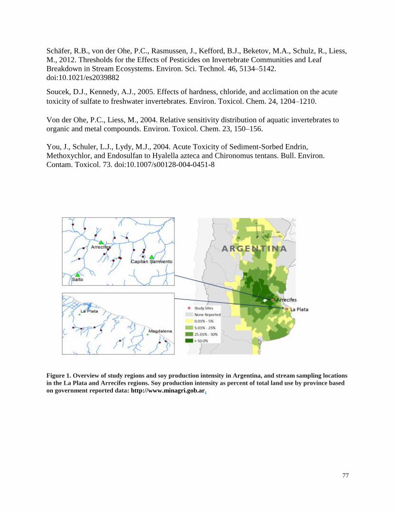
77
Schäfer, R.B., von der Ohe, P.C., Rasmussen, J., Kefford, B.J., Beketov, M.A., Schulz, R., Liess,
M., 2012. Thresholds for the Effects of Pesticides on Invertebrate Communities and Leaf
Breakdown in Stream Ecosystems. Environ. Sci. Technol. 46, 5134–5142.
doi:10.1021/es2039882
Soucek, D.J., Kennedy, A.J., 2005. Effects of hardness, chloride, and acclimation on the acute
toxicity of sulfate to freshwater invertebrates. Environ. Toxicol. Chem. 24, 1204–1210.
Von der Ohe, P.C., Liess, M., 2004. Relative sensitivity distribution of aquatic invertebrates to
organic and metal compounds. Environ. Toxicol. Chem. 23, 150–156.
You, J., Schuler, L.J., Lydy, M.J., 2004. Acute Toxicity of Sediment-Sorbed Endrin,
Methoxychlor, and Endosulfan to Hyalella azteca and Chironomus tentans. Bull. Environ.
Contam. Toxicol. 73. doi:10.1007/s00128-004-0451-8
Figure 1. Overview of study regions and soy production intensity in Argentina, and stream sampling locations
in the La Plata and Arrecifes regions. Soy production intensity as percent of total land use by province based
on government reported data: http://www.minagri.gob.ar.

78
Figure 2. Univariate linear regression between total insecticide TUs and community metrics for (a)
SPEARpesticide values of emergent vegetation samples in La Plata and Arrecifes with values averaged over two
sampling events in 2011-2012), (b) SPEARpesticide values of benthos samples in La Plata and Arrecifes with
values averaged over two sampling events in 2011-2012, (c) benthos samples in Arrecifes with values averaged
over two sampling events in 2013-2014, (d) % crustacea values of emergent vegetation samples in La Plata
and Arrecifes with values averaged over two sampling events in 2011-2012), (e) % crustacea values of benthos
samples in La Plata and Arrecifes with values averaged over two sampling events in 2011-2012, and (f) %
crustacea of benthos samples in Arrecifes with values averaged over two sampling events in 2013-2014.
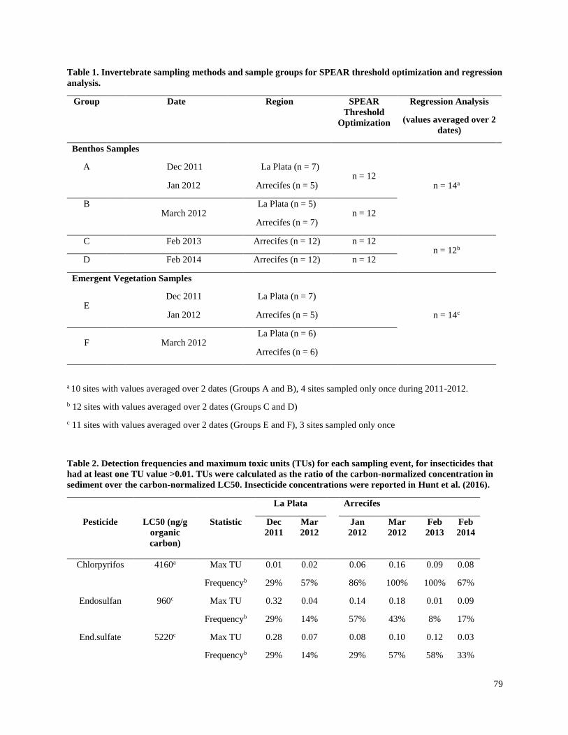
79
Table 1. Invertebrate sampling methods and sample groups for SPEAR threshold optimization and regression
analysis.
Group
Date Region SPEAR
Threshold
Optimization
Regression Analysis
(values averaged over 2
dates)
Benthos Samples
A
Dec 2011 La Plata (n = 7) n = 12
n = 14a
Jan 2012 Arrecifes (n = 5)
B March 2012
La Plata (n = 5) n = 12
Arrecifes (n = 7)
C Feb 2013 Arrecifes (n = 12) n = 12 n = 12b
D Feb 2014 Arrecifes (n = 12) n = 12
Emergent Vegetation Samples
E Dec 2011 La Plata (n = 7)
n = 14c
Jan 2012 Arrecifes (n = 5)
F March 2012 La Plata (n = 6)
Arrecifes (n = 6)
a 10 sites with values averaged over 2 dates (Groups A and B), 4 sites sampled only once during 2011-2012.
b 12 sites with values averaged over 2 dates (Groups C and D)
c 11 sites with values averaged over 2 dates (Groups E and F), 3 sites sampled only once
Table 2. Detection frequencies and maximum toxic units (TUs) for each sampling event, for insecticides that
had at least one TU value >0.01. TUs were calculated as the ratio of the carbon-normalized concentration in
sediment over the carbon-normalized LC50. Insecticide concentrations were reported in Hunt et al. (2016).
La Plata Arrecifes
Pesticide LC50 (ng/g
organic
carbon)
Statistic Dec
2011
Mar
2012
Jan
2012
Mar
2012
Feb
2013
Feb
2014
Chlorpyrifos 4160a Max TU 0.01 0.02 0.06 0.16 0.09 0.08
Frequencyb 29% 57% 86% 100% 100% 67%
Endosulfan 960c Max TU 0.32 0.04 0.14 0.18 0.01 0.09
Frequencyb 29% 14% 57% 43% 8% 17%
End.sulfate 5220c Max TU 0.28 0.07 0.08 0.10 0.12 0.03
Frequencyb 29% 14% 29% 57% 58% 33%

80
Cypermethrin 380a Max TU 0.05 nd 1.15 0.97 0.38 0.13
Frequencyb 29% 0% 29% 29% 33% 8%
L-cyhalothrin 450a Max TU NA 0.02 NA 0.71 0.23 0.16
Frequencyb 0% 29% 17% 0%
Bifenthrin 520d Max TU NA NA NA NA nd 0.36
Frequencyb 0% 17%
Total pyrethroid TU e,g Max TU 0.05 0.05 1.15 1.16 0.45 0.41
Total insecticide TU f,g Max TU 0.66 0.14 1.23 1.36 0.51 0.54
a LC50 for Hyalella azteca from Weston et al. 2013
b Frequency of detection above the highest quantitation limit of 0.5 ng/g dw in sediment.
c LC50 for Chironomus tentans from You et al. 2005
dFrequency of detection above the highest quantitation limit of 0.25 ng/g dw in sediment
e Total pyrethroid TU values for each sample were calculated by summing the TU values for each pyrethroid.
fTotal insecticide TU values for each sample were calculated by summing the TU values for each insecticide.
gA concentration value of half the quantitation limit was assigned for pesticides detected in the sample group but not
detected in the sample, or detected <QL in the sample.
Table 3. Optimized SPEARpesticides thresholds, relative taxa abundance, and univariate regression results.
Response Variable
Univariate Regression Results
Data
Group
Total Insecticide TU Pyrethroid TU
Trenda r2 p-value Trenda r2 p-value
Benthic invertebrate communities
Optimized SPEAR Thresholds
Sensitivity Generation
Time (yr)
SPEARpesticides -0.2 0.5 2011-12 + 0.35 0.03 0.10 0.28
2013-14 + 0.39 0.03 + 0.58 0.004
Community Metrics
mean (min – max)
La Plata Arrecifes
Richness 6.6
(2-15)
12
(3-26)
2011-12 0.24 0.07 0.14 0.19
2013-14 0.09 0.36 0.02 0.68
Diversity 0.90
(0.26-2.2)
1.4
(0.37-2.5)
2011-12 0.14 0.19 0.05 0.46
2013-14 0.10 0.31 0.05 0.47

81
% crustacea 32
(0-96)
6
(0-35)
2011-12 + 0.57 0.002 + 0.35 0.03
2013-14 0.04 0.51 0.09 0.33
% amphipoda 16
(0-83)
5
(0-33)
2011-12 + 0.53 0.003 + 0.36 0.02
2013-14 0.04 0.51 0.09 0.34
%ephemeroptera 1.3
(0-9.0)
23
(0-83)
2011-12 0.00 0.74 0.04 0.49
2013-14 0.01 0.73 0.01 0.74
% trichoptera 0
(0-0)
1.1
(0-16)
2011-12b - - - -
2013-14 0.21 0.14 0.15 0.22
% EPT 1.3
(0-9.0)
24
(0-83)
2011-12 0.00 0.74 0.04 0.49
2013-14 0.00 0.88 0.00 0.86
% diptera 3.1
(0-15)
20
(0-89)
2011-12 0.20 0.11 0.25 0.07
2013-14 0.00 0.99 0.00 0.97
% chironomidae 2.6
(0-15)
19
(0-83)
2011-12 0.22 0.09 0.27 0.06
2013-14 0.00 0.99 0.00 0.95
% oligochaetes 40
(0-91)
16
(0-83)
2011-12 0.20 0.11 0.01 0.70
2013-14 0.00 0.87 0.02 0.70
% bivalvia 2
(0-12)
4
(0-38)
2011-12 0.08 0.32 0.05 0.46
2013-14 0.32 0.05 - 0.47 0.01
% gastropoda 4
(0-17)
16
(0-89)
2011-12 0.01 0.78 0.04 0.49
2013-14 0.01 0.72 0.04 0.54
Vegetation-associated invertebrate communities
Optimized SPEAR Thresholdsc
Sensitivity Generation
Time (yr)
SPEARpesticides -0.2 0.5 2011-12 + 0.42 0.01 0.14 0.19
Community Metrics
mean (min – max)
La Plata Arrecifes
Richness 13(4.3-25) 18(5.3-30) 2011-12 0.05 0.42 0.09 0.28
Diversity 1.4(0.3-2)
1.7(0.8-
2.9)
2011-12 0.17 0.14 0.15 0.17
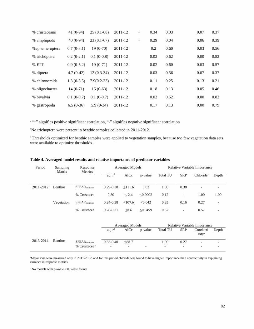
82
% crustaceans 41 (0-94) 25 (0.1-68) 2011-12 + 0.34 0.03 0.07 0.37
% amphipods 40 (0-94) 23 (0.1-67) 2011-12 + 0.29 0.04 0.06 0.39
%ephemeroptera 0.7 (0-3.1) 19 (0-70) 2011-12 0.2 0.60 0.03 0.56
% trichoptera 0.2 (0-2.1) 0.1 (0-0.8) 2011-12 0.02 0.62 0.00 0.82
% EPT 0.9 (0-5.2) 19 (0-71) 2011-12 0.02 0.60 0.03 0.57
% diptera 4.7 (0-42) 12 (0.3-34) 2011-12 0.03 0.56 0.07 0.37
% chironomids 1.3 (0-5.5) 7.9(0.2-23) 2011-12 0.11 0.25 0.13 0.21
% oligochaetes 14 (0-71) 16 (0-63) 2011-12 0.18 0.13 0.05 0.46
% bivalvia 0.1 (0-0.7) 0.1 (0-0.7) 2011-12 0.02 0.62 0.00 0.82
% gastropoda 6.5 (0-36) 5.9 (0-34) 2011-12 0.17 0.13 0.00 0.79
a “+” signifies positive significant correlation, “-” signifies negative significant correlation
bNo trichoptera were present in benthic samples collected in 2011-2012.
c Thresholds optimized for benthic samples were applied to vegetation samples, because too few vegetation data sets
were available to optimize thresholds.
Table 4. Averaged model results and relative importance of predictor variables
Period Sampling Matrix
Response Metrics
Averaged Models Relative Variable Importance
adj r2 AICc p-value Total TU SRP Chloridea Depth
2011-2012 Benthos
SPEARpesticides 0.29-0.38 ≤111.6 0.03 1.00 0.38 - -
% Crustacea 0.80 ≤-2.4 ≤0.0002 0.12 - 1.00 1.00
Vegetation
SPEARpesticides 0.24-0.38 ≤107.6 ≤0.042 0.85 0.16 0.27 -
% Crustacea 0.28-0.31 ≤8.6 ≤0.0499 0.57 - 0.57 -
2013-2014
Benthos
Averaged Models Relative Variable Importance
adj r2 AICc p-value Total TU SRP Conductivitya
Depth
SPEARpesticides 0.33-0.40 ≤68.7 1.00 0.27 - -
% Crustacea b - - - - - - -
aMajor ions were measured only in 2011-2012, and for this period chloride was found to have higher importance than conductivity in explaining
variance in response metrics.
b No models with p-value < 0.5were found
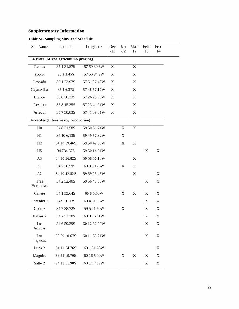
83
Supplementary Information
Table S1. Sampling Sites and Schedule
Site Name Latitude Longitude Dec
-11
Jan
-12
Mar-
12
Feb-
13
Feb-
14
La Plata (Mixed agriculture/ grazing)
Remes 35 1 31.87S 57 59 39.6W X X
Poblet 35 2 2.45S 57 56 34.3W X X
Pescado 35 1 23.97S 57 51 27.42W X X
Cajaravilla 35 4 6.37S 57 48 57.17W X X
Blanco 35 8 30.23S 57 26 23.98W X X
Destino 35 8 15.35S 57 23 41.21W X X
Arregui 35 7 38.83S 57 41 39.01W X X
Arrecifes (Intensive soy production)
H0 34 8 31.58S 59 50 31.74W X X
H1 34 10 6.13S 59 49 57.32W X
H2 34 10 19.46S 59 50 42.60W X X
H5 34 734.67S 59 50 14.31W X X
A3 34 10 56.82S 59 58 56.13W X
A1 34 7 28.59S 60 3 30.76W X X
A2 34 10 42.52S 59 59 23.43W X X
Tres
Horquetas
34 2 52.40S 59 56 40.00W X X
Canete 34 1 53.64S 60 8 5.50W X X X X
Contador 2 34 9 20.13S 60 4 51.35W X X
Gomez 34 7 38.72S 59 54 1.50W X X X
Helves 2 34 2 53.30S 60 0 56.71W X X
Las
Animas
34 6 59.39S 60 12 32.90W X X
Los
Ingleses
33 59 10.67S 60 11 59.21W X X
Luna 2 34 11 54.76S 60 1 31.78W X
Maguire 33 55 19.70S 60 16 5.90W X X X X
Salto 2 34 11 11.90S 60 14 7.22W X X
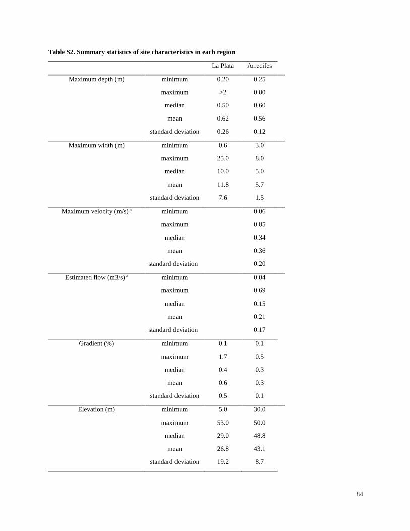
84
Table S2. Summary statistics of site characteristics in each region
La Plata Arrecifes
Maximum depth (m) minimum 0.20 0.25
maximum >2 0.80
median 0.50 0.60
mean 0.62 0.56
standard deviation 0.26 0.12
Maximum width (m) minimum 0.6 3.0
maximum 25.0 8.0
median 10.0 5.0
mean 11.8 5.7
standard deviation 7.6 1.5
Maximum velocity (m/s) a minimum 0.06
maximum 0.85
median 0.34
mean 0.36
standard deviation 0.20
Estimated flow (m3/s) a minimum 0.04
maximum 0.69
median 0.15
mean 0.21
standard deviation 0.17
Gradient (%) minimum 0.1 0.1
maximum 1.7 0.5
median 0.4 0.3
mean 0.6 0.3
standard deviation 0.5 0.1
Elevation (m) minimum 5.0 30.0
maximum 53.0 50.0
median 29.0 48.8
mean 26.8 43.1
standard deviation 19.2 8.7
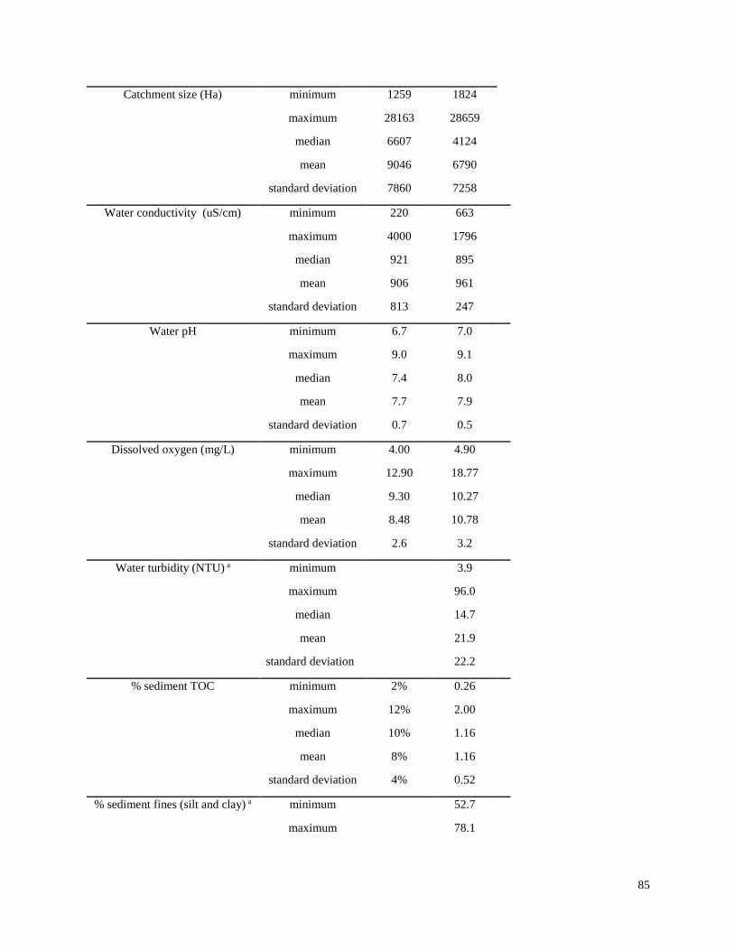
85
Catchment size (Ha) minimum 1259 1824
maximum 28163 28659
median 6607 4124
mean 9046 6790
standard deviation 7860 7258
Water conductivity (uS/cm) minimum 220 663
maximum 4000 1796
median 921 895
mean 906 961
standard deviation 813 247
Water pH minimum 6.7 7.0
maximum 9.0 9.1
median 7.4 8.0
mean 7.7 7.9
standard deviation 0.7 0.5
Dissolved oxygen (mg/L) minimum 4.00 4.90
maximum 12.90 18.77
median 9.30 10.27
mean 8.48 10.78
standard deviation 2.6 3.2
Water turbidity (NTU) a minimum 3.9
maximum 96.0
median 14.7
mean 21.9
standard deviation 22.2
% sediment TOC minimum 2% 0.26
maximum 12% 2.00
median 10% 1.16
mean 8% 1.16
standard deviation 4% 0.52
% sediment fines (silt and clay) a minimum 52.7
maximum 78.1
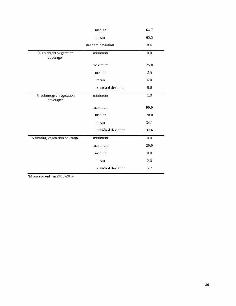
86
median 64.7
mean 65.5
standard deviation 8.6
% emergent vegetation
coverage a
minimum 0.0
maximum 25.0
median 2.5
mean 6.0
standard deviation 8.6
% submerged vegetation
coverage a
minimum 1.0
maximum 90.0
median 20.0
mean 34.1
standard deviation 32.6
% floating vegetation coverage a minimum 0.0
maximum 20.0
median 0.0
mean 2.0
standard deviation 5.7
aMeasured only in 2013-2014.
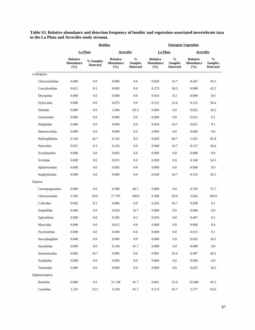
87
Table S3. Relative abundance and detection frequency of benthic and vegetation-associated invertebrate taxa
in the La Plata and Arrecifes study streams.
Benthos Emergent Vegetation
La Plata Arrecifes La Plata Arrecifes
Relative
Abundance
(%)
% Samples
Detected
Relative
Abundance
(%)
%
Samples
Detected
Relative
Abundance
(%)
%
Samples
Detected
Relative
Abundance
(%)
%
Samples
Detected
Coleoptera
Chrysomelidae 0.000 0.0 0.000 0.0 0.020 16.7 0.267 45.5
Curculionidae 0.021 8.3 0.003 0.0 0.273 58.3 0.089 45.5
Dryopidae 0.000 0.0 0.000 0.0 0.010 8.3 0.000 0.0
Dytiscidae 0.000 0.0 0.073 0.0 0.151 25.0 0.153 36.4
Elmidae 0.000 0.0 1.696 83.3 0.000 0.0 0.025 18.2
Georissidae 0.000 0.0 0.000 0.0 0.000 0.0 0.013 9.1
Haliplidae 0.000 0.0 0.000 0.0 0.030 16.7 0.051 9.1
Heteroceridae 0.000 0.0 0.000 0.0 0.000 0.0 0.000 0.0
Hydrophilidae 0.145 16.7 0.132 8.3 0.626 66.7 1.921 81.8
Noteridae 0.021 8.3 0.126 0.0 0.040 16.7 0.127 36.4
Scarabaeidae 0.000 0.0 0.003 0.0 0.000 0.0 0.000 0.0
Scirtidae 0.000 0.0 0.015 0.0 0.020 0.0 0.140 54.5
Sphaeriusidae 0.000 0.0 0.003 0.0 0.000 0.0 0.000 0.0
Staphylinidae 0.000 0.0 0.000 0.0 0.030 16.7 0.153 45.5
Diptera
Ceratopogonidae 0.000 0.0 0.389 66.7 0.000 0.0 0.763 72.7
Chironomidae 2.305 50.0 17.797 100.0 0.384 50.0 3.663 100.0
Culicidae 0.042 8.3 0.006 0.0 0.262 16.7 0.038 9.1
Empididae 0.000 0.0 0.024 16.7 0.000 0.0 0.000 0.0
Ephydidrae 0.000 0.0 0.392 8.3 0.010 0.0 0.407 9.1
Muscidae 0.000 0.0 0.012 0.0 0.000 0.0 0.000 0.0
Psychodidae 0.000 0.0 0.000 0.0 0.000 0.0 0.013 9.1
Sarcophagidae 0.000 0.0 0.000 0.0 0.000 0.0 0.025 18.2
Simuliidae 0.000 0.0 0.144 41.7 0.000 0.0 0.000 0.0
Stratiomyidae 0.062 16.7 0.083 0.0 0.081 25.0 0.407 45.5
Syrphidae 0.000 0.0 0.003 0.0 0.000 0.0 0.000 0.0
Tabanidae 0.000 0.0 0.000 0.0 0.000 0.0 0.025 18.2
Ephemeroptera
Baetidae 0.000 0.0 31.138 41.7 0.061 25.0 16.840 45.5
Caenidae 1.225 33.3 5.258 91.7 0.273 41.7 2.277 63.6
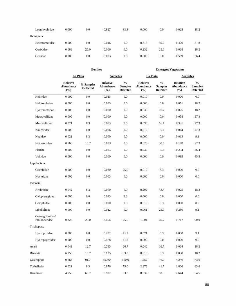
88
Leptohyphidae 0.000 0.0 0.827 33.3 0.000 0.0 0.025 18.2
Hemiptera
Belostomatidae 0.000 0.0 0.046 0.0 0.313 50.0 0.420 81.8
Corixidae 0.083 25.0 0.006 0.0 0.232 25.0 0.038 18.2
Gerridae 0.000 0.0 0.003 0.0 0.000 0.0 0.509 36.4
Benthos Emergent Vegetation
La Plata Arrecifes La Plata Arrecifes
Relative
Abundance
(%)
% Samples
Detected
Relative
Abundance
(%)
%
Samples
Detected
Relative
Abundance
(%)
%
Samples
Detected
Relative
Abundance
(%)
%
Samples
Detected
Hebridae 0.000 0.0 0.015 0.0 0.010 0.0 0.000 0.0
Helotrephidae 0.000 0.0 0.003 0.0 0.000 0.0 0.051 18.2
Hydrometridae 0.000 0.0 0.000 0.0 0.030 16.7 0.025 18.2
Macroveliidae 0.000 0.0 0.000 0.0 0.000 0.0 0.038 27.3
Mesoveliidae 0.021 8.3 0.003 0.0 0.030 16.7 0.331 27.3
Naucoridae 0.000 0.0 0.006 0.0 0.010 8.3 0.064 27.3
Nepidae 0.021 8.3 0.000 0.0 0.000 0.0 0.013 9.1
Notonectidae 0.768 16.7 0.003 0.0 0.828 50.0 0.178 27.3
Pleidae 0.000 0.0 0.083 0.0 0.030 8.3 0.254 36.4
Veliidae 0.000 0.0 0.000 0.0 0.000 0.0 0.089 45.5
Lepidoptera
Crambidae 0.000 0.0 0.080 25.0 0.010 8.3 0.000 0.0
Noctuidae 0.000 0.0 0.003 0.0 0.000 0.0 0.000 0.0
Odonata
Aeshnidae 0.042 8.3 0.000 0.0 0.202 33.3 0.025 18.2
Calopterygidae 0.000 0.0 0.043 8.3 0.000 0.0 0.000 0.0
Gomphidae 0.000 0.0 0.000 0.0 0.010 8.3 0.000 0.0
Libellulidae 0.000 0.0 0.012 0.0 0.061 25.0 0.280 9.1
Coenagrionidae/
Protoneuridae 0.228 25.0 3.454 25.0 1.504 66.7 1.717 90.9
Trichoptera
Hydroptilidae 0.000 0.0 0.202 41.7 0.071 8.3 0.038 9.1
Hydropsychidae 0.000 0.0 0.478 41.7 0.000 0.0 0.000 0.0
Acari 0.042 16.7 0.285 66.7 0.040 16.7 0.064 18.2
Bivalvia 6.956 16.7 5.135 83.3 0.010 8.3 0.038 18.2
Gastropoda 0.664 91.7 15.668 100.0 1.252 91.7 4.236 63.6
Turbellaria 0.021 8.3 0.876 75.0 2.876 41.7 1.806 63.6
Hirudinea 4.755 66.7 0.937 83.3 8.639 83.3 7.644 54.5

89
Nematoda 0.000 0.0 0.251 66.7 0.000 0.0 0.000 0.0
Nemertea 0.000 0.0 0.119 16.7 0.000 0.0 0.000 0.0
Oligochaeta 65.365 58.3 6.801 91.7 4.824 50.0 11.002 45.5
Hydridae 0.000 0.0 0.006 0.0 0.000 0.0 0.000 0.0
Isopoda 0.000 0.0 0.000 0.0 0.182 16.7 0.000 0.0
Decopoda
Palaemonidae 8.181 33.3 0.101 8.3 1.070 33.3 0.445 27.3
Aeglidae 0.000 0.0 0.058 33.3 0.000 0.0 0.000 0.0
Ostracoda 0.145 16.7 0.640 50.0 0.040 16.7 0.509 36.4
Amphipoda
Hyalellidae 8.887 50.0 6.559 66.7 75.454 58.3 42.763 100.0

90
CHAPTER 5
Agricultural stressors affecting invertebrate communities in Atlantic Forest streams,
and mitigation effectiveness of forested riparian buffers

91
Agricultural stressors affecting invertebrate communities in South American Atlantic
Forest streams, and mitigation effectiveness of forested riparian buffers
Abstract
We investigated the influence and relative importance of insecticides and other agricultural
stressors in determining variability in invertebrate communities in small streams in intensive soy
production regions of Brazil and Paraguay. In Paraguay, 17 sites were sampled over two seasons
(January and December 2013), and all sampling sites were on tributaries of the Pirapó River in
the state of Itapúa. In Brazil, 18 sites were sampled once in November 2013, and all sampling
sites were on tributaries of the San Francisco River in the state of Paraná.The riparian buffer
zones generally contained native Atlantic forest remnants and/or introduced tree species at
various stages of growth. Although minimum buffer width in Brazilian streams was negatively
correlated with insecticide concentrations and buffer width was found to have moderate
importance in mitigating effects on some sensitive taxa such as mayflies, insecticides had low
relative importance in explaining variability in invertebrate communities. Paraguay and Brazil
both have laws requiring forested riparian buffers, and the fact that almost all streams had ample
forested riparian buffer zones is likely to have mitigated the effects of pesticides on stream
invertebrate communities in these regions.In Brazilian streams, the percent coverage of soft
depositional sediment in streams was the most important agriculture-related explanatory variable,
and the overall stream habitat score was the most important variable in Paraguay streams.
Introduction
In recent years, soybean production has become a major export crop for multiple countries in
South America, raising concern about environmental impacts. Between 1995 and 2011, soy
cultivation area expanded by 126% in Brazil (Castanheira and Freire 2013). In Paraguay,
soycultivation area increased from 1.3 Mha in 2000-2001 to 2 Mha in 2007-2008 (Garcia-Lopez
and Arizpe 2010). Land use changes caused by this expansion of soy cultivation are likely to
have multiple adverse environmental effects, including reductions in ecosystem complexity, loss
of biodiversity, deforestation, increased erosion, adverse effects of agrochemicals, and increased
greenhouse gas emissions (Botta et al. 2011; Castanheira and Freire 2013; Lathuilliere et al.
2014).
Conversion of land to intensive agriculture can result in degradation of adjacent streams and
stream ecosystem through impacts such as nutrient enrichment, sedimentation, pesticide toxicity,
and deforestation (Gücker et al., 2009; Jones et al., 2001; Matthaei et al., 2010). For example, in
headwater streams of the Brazilian Cerrado, agricultural streams had higher nutrients, reduced
channel morphology, higher velocities, lower microbial biomass, and lower community
respiration compared to less disturbed streams (Gücker et al., 2009). Moreover, in a multiple-
watershed study that evaluated influence of landscape variables on sediment and nutrient load,
amount of agriculture explained 50% of the variation in total nitrate concentrations (Jones et al.,
2001).
Agriculture adjacent to streams can adversely impact benthic macroinvertebrate communities
through multiple mechanisms. Agriculture-related stressors can include habitat degradation (e.g.
92
loss of cover, deposition of fine sediments), hydrological modification (e.g. channelization, less
diversity in pool/run/riffle regimes) and impacts to water quality (e.g. pesticide toxicity, nutrient
eutrophication, increased turbidity and conductivity) (Matthaei et al., 2010; Stehle and Schulz,
2015; Stone et al., 2005; Whiles et al., 2000). Moreover, pesticides used in agriculture can have
severe impacts on stream water quality and ecosystems, and the insecticides used in soy
production in South America are known to be especially toxic to aquatic invertebrates (Hunt et
al., 2016; Mugni et al., 2011). A recent meta-analysis of 838 studies across 73 countries found
that over 50% of measured insecticide concentrations in water bodies exceeded regulatory
threshold levels for surface waters or sediments (Stehle and Schulz, 2015), and another analysis
of data from Europe and Australia reported that pesticides reduced both species and family
richness of aquatic invertebrate communities (Beketov et al., 2013).
As a management strategy, stream buffer width may be one of the most important factors in
mitigating transport of pesticides, sediment,and other pollutants to streams in agricultural areas
(Bunzel et al., 2014; Jones et al., 2001; Rasmussen et al., 2011; Stone et al., 2005), and recent
regulations in both Brazil and Paraguay require forested riparian buffer zones. For example, in
Paraguay, Resolution 485/03 by the Ministry of Agriculture requires a protected zone of 100 m
around all water bodies. In Brazil, a new forest code was approved in 2012 (Law No.12.651/12)
establishing that riparian buffer zone requirements should vary with the general use of the land
adjacent to the water body, the aquatic environment, the stream width, and the size of the rural
property. As a general rule for stream widths of 10 m or less, the legislation requires a buffer
width of 15 m of native riparian forest in rural areas or 30 m if in areas newly converted for rural
activities.
The objectives of the present study were to evaluate: (1) the relative importance of pesticides and
other agriculture-related stressors in explaining variation in invertebrate community metrics in
Atlantic forest streams; and (2) the effectiveness of forested riparian buffer zones in mitigating
adverse effects on streamsof this region.
Study Locations and Sampling Schedule
The study sites included small streams that flowed through agricultural fields in two intensive
soy production regions in the former Atlantic forest habitat of Brazil and Paraguay (Figure 1). In
Paraguay, 17 sites were sampled over two seasons (January and December 2013), and all
sampling sites were on tributaries of the Pirapó River in the state of Itapúa. In Brazil, 18 sites
were sampled once in November 2013, and all sampling sites were on tributaries of the San
Francisco River in the state of Paraná. Both study watersheds were on tributaries of the Paraná
River.
Streams selected for the present study were not artificially channelized, and had a minimum
buffer strip width of at least 3 m between the stream and the adjacent crop fields. The riparian
buffer zones generally contained native Atlantic forest remnants and/or introduced tree species at
various stages of growth. Stream depths ranged from 0.12m to 0.81m, and widths ranged from
2m to 8.5m (Table 1; Table S2).
Stream sampling was timed to occur during or soon after peak insecticide application periods,
which varied depending on planting time. For example, soy can either be planted as an early
season crop or a late season crop. The early season crop was generally planted in September or
October and harvested in January. The late season crop was typically planted between December
93
and February and harvested several months later. Peak insecticide applications for soy production
usually occurred in November and December.
Physico-chemico, habitat and geographical variables
At each sampling site, pH, conductivity, dissolved oxygen, and temperature were measured
during each sampling event with a Yellow Springs Instruments SI 556 multi-parameter probe
(Yellow Springs, OH, USA). Turbidity was measured with a portable turbidity meter (Hanna
Instruments 93414, Woonsocket, RI, USA). Field test kits were used to measure concentrations
of ammonium/ammonia (Sera, Germany), ortho-phosphate (CHEMets K-8510, Midland, VA,
USA), and nitrate nitrogen (LaMotte 3354-01, Chestertown, MD). Sediment samples were
collected for sediment grain size analysis, and organic carbon analysis by ferrous sulfate titration
(USDA 1996).
At each site visit, maximum stream width and depth were measured, and maximum and average
water velocities were measured with a current meter (Global Water FP311, College Station, TX,
USA). Habitat quality was assessed at each site according to the USEPA Rapid Bioassessment
Protocol (Barbour et al., 1999) and assigned a score on a scale of 0 to 200. Minimum buffer
widths were measured immediately upstream of sampling sites, and confirmed with LANDSAT
images. Catchments were delineated in GIS using topographical contours to estimate catchment
size, and the percent forest and percent agriculture within each catchment were estimated using
LANDSAT images. Elevation and stream gradient immediately upstream of each site was
estimated based on topographical contours.
Sediment sample collection and insecticide analysis
The methods for sediment sample collection and analysis of insecticides have been previously
described (Chapter 2). Briefly, composite sediment samples were prepared from 3 to 5 locations
at each site, and insecticides were extracted from sediments by sonication (You et al., 2008).
Samples were analyzed for pyrethroid insecticides, organochlorinated insecticides, and the
organophosphate insecticide chloryrifos by either gas chromatography-electron capture detection
(GC-ECD) or gas chromatography – mass spectrometry – negative chemical ionization (GC-MS-
NCI).
Toxic unit calculation
Insecticide toxic units (TUs) were calculated for all sediment samples:
TU = Ci /EC50i
where Ci was the insecticide concentration in sediment normalized for total organic carbon
(TOC), and EC50iwas the 10-d median effects concentration (LC50) for each insecticide.
The sediment LC50 values for freshwater aquatic invertebrates were identified for sensitive
species (Table 2; Chapter 2). Most of the LC50 values used in the present study were for the
amphipod Hyalella azteca, which is known to be very sensitive to pyrethroids and chlorpyrifos
(Weston and Lydy 2010). Although H. azteca does not occur in Brazil or Paraguay, the closely
related H. curvispina complex occurs throughout South America (Dominguez and Fernandez,
2009), and the pesticide sensitivity of H. curvispina has been shown to be similar to that of H.
azteca (Mugni et al., 2013; Hunt, unpublished data). For endosulfan, the LC50 for the more
94
sensitive Chironomus tentans was used to calculate TUs, because it is substantially lower than
the LC50 for H. azteca (You et al., 2004). Toxicity of pesticides in sediment is highly dependent
on organic carbon content; therefore, the concentrations were normalized for total organic carbon
to calculate TU values.
TU values for all insecticides were summed to calculate total insecticide TUs, and TU values for
all pyrethroid insecticides were used to calculate total pyrethroid TUs. When summing TU
values, all insecticides that were detected in the data set were included, assigning a concentration
of half the quantification limit for pesticides that were not detected in the sample, or detected
below the reporting limit. Insecticides that were measured but not detected in the sample group
were not included in TU calculation.
Macroinvertebrate collection and identification
Benthic macroinvertebrate samples were collected by kick-sampling with a 30cm D-frame dip
net with 500 µm mesh (Wildco, Yulee, FL, USA). With each net placement, the substrate was
disturbed approximately 0.5m upstream of the net. For the first sampling event in Paraguay, three
kick samples, each collected for a period of 30 s, were composited from each site, and all
invertebrates from the composite sample were sorted and identified. At four sites, six additional
30s kick samples were collected several days later because of very low organism counts in the
first sampling event. For subsequent sampling events in Paraguay and Brazil, sample size was
increase to ensure a sufficient number of organisms in each sample, and a subsampling method
was used. A larger sample was obtained at each site (30 kick samples, each collected for a period
of 20 s), and the sample material was homogenized and divided into 24 quadrats. Organisms
from randomly selected quadrats were sorted until a total count of 500 organisms per sample was
reached, or until organisms from all quadrats were sorted. This is close to the upper range of
counts used in US biomonitoring programs involving fixed-numbers of organisms (Carter and
Resh, 2013). Once initiating the sorting of a quadrat, it was finished to completion even if the
target of 500 organisms was reached before finishing the quadrat.
All samples were preserved in the field in 80% ethanol, later sieved (500 µm) in the laboratory,
sorted under 3X magnification, and identified under a stereoscopic microscope. Insects, decapods
and amphipods were generally identified to family, genus, or species level, and other taxa were
identified by higher taxonomic groups (oligochaetes, nemerteas, turbellarias, leeches, nematodes,
gastropods, bivalves) using keys from Dominguez and Fernandez (2009) and Merritt and
Cummins (2008).
SPEARpesticides index
The Species at Risk pesticide index (SPEARpesticides) was developed in Europe to evaluate effects
of pesticides on benthic macroinvertebrate communities(Liess and Ohe, 2005), and has been
applied successfully in several continents (Schäfer et al., 2012). We recently applied the
SPEARpesticides index in streams located in soy production regions of Argentina, and found that it
performed reasonably well (r2 = 0.35 to 0.42) with only minor modifications consisting of
adjusting the sensitivity thresholds for life history traits (Chapter 4).
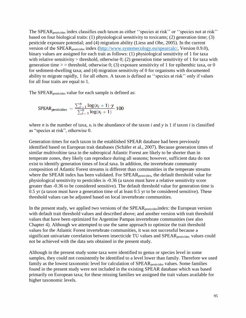
95
The SPEARpesticides index classifies each taxon as either ‘‘species at risk’’ or ‘‘species not at risk’’
based on four biological traits: (1) physiological sensitivity to toxicants; (2) generation time; (3)
pesticide exposure potential; and (4) migration ability (Liess and Ohe, 2005). In the current
version of the SPEARpesticides index (http://www.systemecology.eu/spearcalc/, Version 0.9.0),
binary values are assigned for each trait as follows: (1) physiological sensitivity of 1 for taxa
with relative sensitivity > threshold, otherwise 0; (2) generation time sensitivity of 1 for taxa with
generation time > = threshold, otherwise 0; (3) exposure sensitivity of 1 for epibenthic taxa, or 0
for sediment-dwelling taxa; and (4) migration sensitivity of 0 for organisms with documented
ability to migrate rapidly, 1 for all others. A taxon is defined as ‘‘species at risk’’ only if values
for all four traits are equal to 1.
The SPEARpesticides value for each sample is defined as:
where n is the number of taxa, xi is the abundance of the taxon i and y is 1 if taxon i is classified
as “species at risk”, otherwise 0.
Generation times for each taxon in the established SPEAR database had been previously
identified based on European trait databases (Schäfer et al., 2007). Because generation times of
similar multivoltine taxa in the subtropical Atlantic Forest are likely to be shorter than in
temperate zones, they likely can reproduce during all seasons; however, sufficient data do not
exist to identify generation times of local taxa. In addition, the invertebrate community
composition of Atlantic Forest streams is different than communities in the temperate streams
where the SPEAR index has been validated. For SPEARpesticides, the default threshold value for
physiological sensitivity to pesticides is -0.36 (a taxon must have a relative sensitivity score
greater than -0.36 to be considered sensitive). The default threshold value for generation time is
0.5 yr (a taxon must have a generation time of at least 0.5 yr to be considered sensitive). These
threshold values can be adjusted based on local invertebrate communities.
In the present study, we applied two versions of the SPEARpesticidesindex: the European version
with default trait threshold values and described above; and another version with trait threshold
values that have been optimized for Argentine Pampas invertebrate communities (see also
Chapter 4). Although we attempted to use the same approach to optimize the trait threshold
values for the Atlantic Forest invertebrate communities, it was not successful because a
significant univariate correlation between insecticide TU values and SPEARpesticides values could
not be achieved with the data sets obtained in the present study.
Although in the present study some taxa were identified to genus or species level in some
samples, they could not consistently be identified to a level lower than family. Therefore we used
family as the lowest taxonomic level for calculation of SPEARpesticides values. Some families
found in the present study were not included in the existing SPEAR database which was based
primarily on European taxa; for these missing families we assigned the trait values available for
higher taxonomic levels.
96
Additional bioassessment metrics
In addition to the SPEARpesticides index, we calculated the relative abundance metrics of taxa
groups that were selected based on their common occurrence in the region, and/or known high
sensitivity or tolerance to pesticides and other pollutants (Table S3) (Chang et al., 2014; Rubach
et al., 2010). We also calculated metrics that are used by the local environmental protection
agency in Toledo, Brazil including modified Biological Monitoring Working Party (BMWP)
scores and average score per taxon (BMWP ASPT) (Daniel Buss, personal communication).
Other metrics we calculated included total taxa density per m2, relative abundance of three most
dominant taxa,Shannon-Weaver diversity index,total taxa richness, coleoptera family richness,
trichoptera family richness, and EPT family richness (Table S3). Samples containing more than
300 organisms were rarefied to a constant size of 300 organisms to reduce the effect of sample
size (Barbour and Gerritsen, 1996).
Data analysis
We used several statistical methods to evaluate the relationships between environmental
variables and invertebrate communities. Because riparian buffer zones are expected to have a
protective effect on invertebrate communities through multiple mechanisms, we first evaluated
relationship of buffer width with habitat metrics and water and sediment quality parameters. We
then used univariate regression to evaluate the performance of the indices, and finally applied
multiple regression analysis to evaluate the relative importance of each predictor in explaining
invertebrate community metrics. All data analyses were carried out in the open-source statistical
software R version 3.2.2(R Development Core Team, 2015).
Principle component analysis (PCA) ordination was used to examine patterns in environmental
variables for the two study regions and for the high and low buffer width groups. Environmental
parameters examined in the PCA included all variables in Table S2, with the exception of water
pH, temperature, and dissolved oxygen. pH was not included because of little variation, and DO
and temperature were not included because they depend in part on the time of day that sampling
was conducted.The R function prcomp was used to carry out the PCA, and data for all variables
were centered and scaled prior to analysis.
Non-metric multi-dimensional scaling (NMDS) ordination was used to visually examine patterns
in community structure and environmental variables for the two study regions, and for high and
low buffer width groups (>50m and <50m). The function metaMDS in the vegan package in R
was used to carry out the NMDS ordination, using Bray-Curtis distance. All taxa counts were
square root transformed, and data were standardized using Wisconsin double standardization.
We then used the BIO-ENV procedure (Clarke and Ainsworth, 1993) to identify the subset of
environmental variables that best explain the variation in community composition. Because the
NMDS analysis indicated that community structure was distinct for each of the two regions, we
did this analysis separately for each region. BIO-ENV finds the optimum correlation between a
community dissimilarity matrix and multiple environmental dissimilarity matrices, with all
possible combinations of environmental variables. For the community matrix, we used Bray-
Curtis distance, and for the environmental variable matrix we used Euclidean distance. For
Paraguay sampling sites, when environmental variable values were measured during both
sampling events, average values were used, and invertebrate data collected during two sampling

97
events at the same site were combined. NMDS, correlation analyses, and BIO-ENV were carried
out using the vegan package in R (Oksanen et al., 2013).
Multiple regression analysis was conducted for each of the 31 invertebrate community metrics
(Table S3). Because the NMDS analysis indicated that community structure was distinct for each
of the two regions, we performed the analysis separately for the Paraguay and Brazil data sets,
and variable values for Paraguay were averaged over the two sampling events.For the full
models, we selected the parameters that are both likely to be affected by adjacent agriculture, and
to have an effect on invertebrate communities. Thse parameters included mainly habitat,
substrate, and sediment quality predictor variables (RBP score, % riffles, %TOC in sediment, %
large woody debris (LWD), % fine particulate organic matter (FPOM), % course particulate
organic matter (CPOM), % soft depositional sediment coverage, total insecticide TU (log
transformed) and % sediment fines (only in Brazil because sufficient data were not available for
all sites in Paraguay). Turbidity was also included, but other water quality parameters
(conductivity, pH, temperature) were not included, either because they did not vary much within
regions or depended on the time of day sampled. To evaluate the effect of land use and buffer
width, we also included % agriculture and buffer width as predictor variables, and to account for
the effect of watershed characteristics we included catchment size and elevation.
To avoid using predictor variables with high collinearity, we used a correlation matrix to select
variables that were highly correlated with response variables but not with other predictor
variables. After initial variable selection, we checked variance inflation factors (VIFs) with the
full model to avoid high collinearity (“vif” function in R package “cor”). All predictor variables
had VIF values less than three.
We then selected the best predictive models based on Akaike information criterion values
corrected for small sample size (AICc) and p-values (Barton, 2015). The AICc for each model
was calculated as the difference between the AICc for the model and the lowest AICc of all
models. For each predictor variable in selected models with AICc < 4 and p-value < 0.05, we
determined the magnitude and direction of coefficients using multi-model averaging across
selected models (Grueber et al., 2011) using the dredge and model.avg functions in the R
package MuMIn version 1.15.1 (Barton, 2015). Relative importance of each predictor variable
was calculated as the relativized sum of the Akaike weights over all of the selected models
containing the variable of interest (Barton, 2015). Importance ranged from 0 (i.e. parameter not
given any explanatory weight in any of the selected model) to 1 (i.e. parameter included in all
selected models).
We then used simple linear regressions to analyze the effect of agriculture and buffer width on
each of the habitat, substrate, and sediment and water quality parameters that were shown to have
high importance in invertebrate community response metrics.
Results
Insecticides Present
In both regions, the most commonly detected insecticide was chlorpyrifos, followed by the
pyrethroids cypermethrin, lambda-cyhalothrin, bifenthrin, cyfluthrin, deltamethrin, esfenvalerate
and permethrin (Table 2). Although chlorpyrifos was detected in most samples, it is less potent

98
than the pyrethroid insecticides, and the maximum TU values for chlorpyrifos were lower than
the total pyrethroid TU values. Endosulfan and its degradate endosulfan sulfate were detected
occasionally, but with relatively low TU values. The banned organochlorine insecticides DDT
(and degradates), endrin, chlordane, and aldrin were also detected in some samples, but TU
values were always below 0.01. The total insecticide and total pyrethroid TU values were highly
correlated, and were similar between the two regions(Hunt et al. 2016).
Water and sediment quality
The PCA ordinationshowed that the Paraguay and Brazil sites were clearly distinct on the
horizontal axis with respect to certain water quality and sediment quality parameters (organic
carbon, % fine sediment, conductivity), but similar with respect to others (insecticide TU values,
% soft sediment, and turbidity) (Figure 2a, d). Generally, percent fine sediments and organic
carbon were higher in Brazil than in Paraguay (Table S2), and conductivity was higher in
Paraguay than in Brazil (Table S2).
The low and high buffer groups were partially overlapping, but slightly separated with regard to
parameters on the vertical axis (insecticide TU values, turbidity, and to a lesser extent, % fines
and soft sediment) (Figure 2b, d). When split into high and low buffer zone groups by region, the
low and high groups were still distinct from each other within each region (Figure 2c), indicating
that the differences in pesticide TU values, % soft sediment, and turbidity are more likely to be
related to differences in buffer width than to differences between the two regions.
The nutrient results indicated that nutrient concentrations were in the lowest concentration
categories (ammonia/ammonium < 0.5 ppm, nitrates < 1 ppm, ortho-phosphate < 0.1 ppm) for all
or most sites in both regions. Four sites in Brazil and five sites in Paraguay had nitrate
concentrations of 1-2 ppm, and two sites in Brazil had ortho-phosphate concentrations between
0.1-0.2 ppm. Because nutrients concentrations were generally low and did not vary much
between sites, nutrients were not included as variables in the statistical analyses.
Habitat quality and landscape characteristics
The PCA ordination showed that the Brazil and Paraguay sampling sites were distinct with
respect to certain habitat quality parameters along the vertical axis (Figure 3a, d). Generally,
Brazil sites tended to have higher particulate organic matter and large woody debris, and more
riffles, while Paraguay sites tended to have a higher percentage of forest in catchment areas,
larger buffer zones, and more bedrock and runs in streams (Figure 3, Table 1). However, the
overall RBP habitat scores were similar for both regions (Table 1).
The low and high buffer groups were also clearly distinct from each other with regard to the
same parameters on the vertical axis that separated the regions (Figure 3b, d). However, when
split into low and high buffer zone groups by region, the buffer groups within each region
overlapped with each other (Figure 3c), indicating that the differences in habitat quality were
primarily an artifact of the differences in the regional data sets, and not a result of buffer size.
In addition to the differences in habitat parameters, Brazil and Paraguay sampling sites were also
distinct with respect to catchment landscape characteristics. Catchment sizes of the Paraguay
sites tended to be larger than those in Brazil, hence the stream widths and depths were also
generally larger. Elevations of all sites in Brazil were higher than those at Paraguay sites, and
99
stream gradients tended to be slightly higher in Brazil but were not significantly different
between regions (Table 1).
Invertebrate community analysis
Invertebrate community composition was similar in the two regions, but there were some
differences in relative abundance of certain groups, and in families present (Table S4; Figure 4).
In Paraguay samples, we identified a total of 49 insect families, including 13 families which were
not present in samples collected from Brazil sites (Table S4). In Brazil samples, we identified a
total of 38 insect families, two of which were not present in samples collected from Paraguay
sites. All of the insect families that were found in one region but not the other occurred only
rarely in the region where they were detected (< 1% relative abundance). In Paraguay, the only
decapod found was Trichodactylidae, and in Brazil the only decapod found was Aeglidae. No
ostracods were found in Paraguay samples, but they were found in very small numbers at two
sites in Brazil.
In both regions, the dominant family was Chironomidae (Diptera), but relative abundance was
substantially higher in Brazil (Table S3). The second most dominant family in both regions was
Elmidae (Coleoptera), and in this case relative abundance was higher in Paraguay. In Paraguay,
Leptohyphidae was the most common Ephemeroptera family, while in Brazil, Leptophlebiidae
was most common. In Paraguay, trichopterans had higher relative abundance and more families
present than in Brazil. Plecopterans were rare in both regions.
The NMDS results indicated that the invertebrate communities were distinct between Brazil and
Paraguay (Figure 4a), but not between low and high buffer groups (Figure 4b). However, the
stress values for the NMDS analysis done in two dimensions was somewhat high for the Brazil
data set (0.20) as well as the combined Brazil and Paraguay data set (0.23), indicating that the
results should be interpreted only for identifying rough patterns. For the Paraguay data set, stress
was lower (0.13).
The BIO-ENV analysis indicated that for the Paraguay data set, only two variables were
important in explaining variation in invertebrate communities: stream width and RBP habitat
quality score (r = 0.42). However, for the Brazil data set, the maximum correlation between
community and environmental dissimilarity matrices (r=0.39) was obtained when 10 variables
were included in the model: conductivity, turbidity, % soft sediment, % bedrock, % CPOM,
buffer width, site elevation, stream gradient, stream width, and stream depth.
Community metrics and relative importance of predictor variables
In both regions, multiple significant models (p-value < 0.05) were selected for four community
metrics: %EPT, %EPT-HB, % ephemeroptera and % trichoptera. In Brazil, one additional metric
(coleoptera richness) had significant models, and in Paraguay nine additional metrics had
significant models (Table 3).
In both regions, % agriculture had moderate to high importance (>0.4) and significant effect
(average p-value < 0.05) on %EPT, with a negative influence (Table 3). In Brazil, % agriculture
also significantly and adversely affected % Ephemeroptera, but in Paraguay, % agriculture had
no importance in explaining variability in % Ephemeroptera. In Brazil, % agriculture had a
negative relationship with %EPT-HB, % Trichoptera, and Coleoptera richness, but with low
100
importance (< 0.4) and average p-value > 0.05. In Paraguay, % agriculture had a negative
relationship with the ASPT index, with moderate importance (0.46), but average p-value > 0.05.
In Brazil, buffer width appeared to have a mitigating effect, but this relationship was not
discernable in Paraguay where most of the sites had mimimum buffer width of 100m or greater.
Buffer width had a positive influence and moderate importance on both %EPT-HB and %
ephemeroptera in Brazil, but was significant (average p-value > 0.05) only for % Ephemeroptera.
In Paraguay, buffer width exhibited little or no importance on all response metrics evaluated
(Table 3).
Insecticide TU values did not appear to have an explanatory role for the SPEARpesticides index or
other invertebrate community metrics in either region. In Brazil, insecticide TU had little or no
importance for all response metrics. In Paraguay, insecticide TU did have high importance and a
significant relationship for two metrics (% Ephemeroptera and the ASPT index), but the positive
direction was opposite to the expected relationship. The SPEARpesticides index values were not
significantly correlated with insecticide TU values in either region. In Paraguay, several habitat
parameters were the only predictor variables that were important in explaining variability in
SPEARpesticides index values. In Brazil, none of the parameters included in the model were
significantly correlated with SPEARpesticides index values.
Overall, RBP habitat score was the most important parameter in Paraguay, but was not a good
explanatory variable in Brazil. In Paraguay, RBP habitat score had high importance and was
significant for eight response metrics, always in the expected direction (positive coefficient for
seven sensitive response metrics, and negative for relative abundance of the dominant taxon).
However, RBP habitat score had no significant effect (average p-value < 0.05) for any response
metric in Brazil, and coefficients for three sensitive response metrics were negative (the opposite
direction as expected).
With regard to substrate and water quality parameters, % soft depositional sediment coverage
was the best predictor variable in Brazil, but its influence in Paraguay was mixed. In Brazil, this
parameter had a significant negative effect with moderate to high importance for three response
metrics. However, in Paraguay, while the effect was usually as expected (negative for sensitive
response metrics %EPT-HB and SPEAR, and positive for relative abundance of three most
dominant taxa) it was not as expected for one metric (positive relationship with rare and sensitive
taxa). Several other parameters (% riffles, turbidity, course and fine particulate matter, large
woody debris, and sediment TOC) had moderate to high importance and were significant for
some response metrics, but effects were not always consistent within or between regions (Table
3).
Although adjacent agriculture would be expected to result in increased deposition of soft
sediment in streams and degradation of habitat quality, the effect of % agriculture on % soft
sediment coverage and on RBP habitat score was not statistically significant in either region.
Similarly, there was no statistically significant relationship between buffer width and % soft
sediment coverage or RBP habitat score, although the relationship in Paraguay was close to
significant (p = 0.053) for soft sediment coverage.
With respect to landscape parameters, catchment area was most important in Brazil, and stream
gradient was most important in Paraguay. Generally, catchment area showed a positive
relationship with sensitive metrics, while gradient had a negative relationship with sensitive
101
metrics and positive relationship with relative abundance of dominant taxa. In Brazil, catchment
size was the most important predictor variable in explaining variability in %EPT-HB and %
ephemeroptera.
Discussion
Relative importance of agricultural stressors
While percent of soft sediment coverage had high importance in determining variability in
multiple community metrics in both of our study regions, the RBP habitat score was important
only in the Paraguay region. The RBP habitat score was also one of only two parameters
determined to be important in determining community structure in Paraguay by the BIO-ENV
analysis. When we examined each of the 10 parameters that comprise the total RBP habitat score,
we found that for the Paraguay data set, the parameters that contributed most variation to the total
score were primarily those related to substrate, including embeddedness, sediment deposition,
and riffle frequency. Bank stability also contributed highly, and generally corresponded with
sediment deposition and embeddedness. There was little variation in scores for flow and channel
alteration, as the study streams were generally not altered.
Our study’s findings that stressors relating to stream substrate were the most important in
determining invertebrate community structure correspond with results fromprevious studies
(Richards et al., 1993; Wood and Armitage, 1997). For example, Richards et al. (1993) found
that the most important morphological factors affecting invertebrate communities in streams in
an agriculture-dominated region were related to substrate composition and fine sediment
distribution. In addition to changing the type of substrate available to invertebrates, deposition of
fine sediment can alter stream morphology and decrease structural diversity of stream habitat by
filling pools and covering hard surfaces such as rocks (Richards et al., 1993; Wood and
Armitage, 1997).
None of the analyses conducted in the present study indicated that insecticides were important in
determining invertebrate community structure in either region. Insecticide TU levels were not
determined to be important either in the BIO-ENV analysis, or in the multiple regression analysis
using various bioassessment metrics. The SPEARpesticides index has been shown to be a sensitive
indicator of pesticide effects on invertebrate communities in many different regions of the world
(Schäfer et al., 2012), but was not correlated with insecticide levels in the present study. Unlike
other bioassessment indices, the SPEARpesticides index has been shown to respond selectively to
pesticide stressors and to be relatively insensitive to most other stressors, although its
performance can be affected by severe habitat degradation (siltation and channelization) and low
dissolved oxygen (Liess and Ohe, 2005; Jes Jessen Rasmussen et al., 2011; Schäfer et al., 2011,
2007).
There are several factors that may help explain why SPEARpesticides index values were not
significantly correlated with insecticide TU values in either of the Atlantic forest regions we
studied. First, the presence of forested riparian buffers along their entire lengths of all streams is
likely to increase the resilience and recovery ability of invertebrate communities. Second, the
sensitive taxa groups found in the study streams are likely to be sensitive to many habitat and
water quality variables in addition to pesticides, potentially confounding the analysis. Third, the
SPEARpesticides index may not work well in tropical and subtropical environments without
significant adaptation.

102
There is ample evidence that forested headwaters provide reservoirs of invertebrate populations
that assist in the recovery of downstream communities after disturbance from pesticide exposure
(Liess and Ohe, 2005; Orlinskiy et al., 2015). For example, a study in an agricultural region of
Germany found that upstream forested headwaters mitigated the effects of pesticides on
downstream invertebrate populations (Orlinskiy et al., 2015). In streams in intensive soy
production regions of Argentina, we found similar upper levels of insecticides as in the Brazil
and Paraguay study regions, but in Argentina the insecticides were more clearly correlated with
impacts on sensitive invertebrate taxa (Chapter 4). A possible reason for the difference may be
that the stream buffers in Argentina were much smaller and were not forested, thus the
invertebrate communities were not as resilient.
In contrast to the Atlantic Forest streams included in the present study, invertebrate communities
in streams of the Argentine Pampas tend to contain large percentages of amphipods, which are
very sensitive to pesticides but relatively tolerant of many habitat and water quality parameters
(Chapters 3 and 4). When the SPEAR index threshold values were optimized for Argentine
Pampas streams, only the crustaceans and trichopterans were considered sensitive to pesticides,
and amphipods were the most abundant sensitive organisms, making them very important in the
performance of the SPEARpesticides index. In the Atlantic Forest streams, amphipods and other
crustaceans were rare, and other sensitive and abundant taxa (such as EPT taxa) tend to be
sensitive not only to pesticides but also to many habitat and water quality parameters (Bunzel et
al., 2013).
The SPEARpesticides index has not yet been validated for tropical or subtropical streams. A study
in tropical streams of Costa Rica did not find a correlation between pesticide toxic units and a
modified version of SPEAR (Rasmussen et al., 2016). However, that study measured only three
sites, and all sites suffered from low dissolved oxygen and lacked sensitive taxa. The
inconclusive finding with SPEAR may be a result of the study design, including factors such as
low number of sampling sites, narrow environmental gradient, and many confounding factors.
Although it is possible that the SPEARpesticides index may not work well in tropical or subtropical
environments without significant modification, more study is necessary to determine this.
Influence of forested riparian buffers
The present study’s findings in Brazil corroborate findings from other studies that have found
riparian buffer zones to be important in mitigating transport of pesticides to streams (Rasmussen
et al. 2011; Di Marzio 2010; Bunzel et al. 2014; Reichenberger et al. 2007; Aguiar et al., 2015).
Another study of Atlantic Forest streams in Brazil found no pesticides except the herbicide
atrazine in streams with a forested buffer of approximately 60m, while multiple pesticides
including chlorpyrifos and lambda-cyhalothrin were detected in streams with 12m and 36m of
forested buffer width (Aguiar et al., 2015). Buffers comprised of grass or shrubs were not as
effective in pesticide removal as forested buffers (Aguiar et al., 2015). Many factors could affect
the buffer width needed to protect streams from pesticide exposure, including gradient, type of
vegetation, soil properties, types of pesticides applied, timing and amount of pesticides applied,
and presence of tile drains or drainage ditches that short-circuit the buffer zones (Reichenberger
et al. 2007; Bunzel et al. 2014).

103
The lack of variation in minimum buffer width at the Paraguay sampling sites likely limited a
firm conclusion regarding the influence of buffer width in this region. Approximately half of the
Paraguay sites had minimum buffer widths of 100m, which was the minimum required by law. In
contrast, in the Brazil study region where buffer width did not exhibit the same clustered pattern,
it was the most important variable in explaining insecticide TU values and also had moderate
importance in explaining the variability in several invertebrate community metrics. In Chapter 2 I
reported that highest insecticide toxic units in both study regions occurred when buffer zone
widths were 20 m or less. Moreover, a multiple regression for the Brazil data set indicated that
buffer width was the predictor variable that had the greatest influence on total insecticide TU.
The selected model included the following predictor variables: buffer width, percent total organic
carbon in sediment, and stream gradient (r2 = 0.54; p-value = 0.009). The analysis of relative
importance indicated that buffer width contributed 74% of the explained variance in total
insecticide TU values, with percent total organic carbon and stream gradient contributing 9 and
17 %, respectively.
Because almost all streams in both regions we studied had relatively large forested stream
buffers, it is possible that relative effects of buffer widths in protecting invertebrate communities
were less evident in this study than in other similar studies in which streams generally had much
smaller buffer width. We measured minimum buffer width observed immediately upstream of
each sample site, and confirmed the measurements using LANDSAT images. However, for most
streams, the average upstream riparian buffer width was considerably larger than the minimum
width measured near the sampling site, and forested buffers typically extended throughout the
entire watershed, even around the small headwater streams. Therefore, the streams in the two
regions included in the present study can be considered well protected in comparison to streams
in many intensive agricultural regions. In contrast, previous studies that have found riparian
buffer zones to be effective in mitigating effects on stream invertebrate communities have
generally evaluated streams with much smaller protected buffer zones than those in the present
study. For example, Whiles et al. (2000) found that land use within 18m of streams in
agricultural areas of Nebraska was correlated with invertebrate bioassessment scores. Another
study in Ontario reported that forested area within a 30m riparian zone was positively correlated
with increases in EPT taxa and taxa diversity (Rios and Bailey, 2006). In our Brazil study area,
where buffer widths were generally lower than those in Paraguay, buffer width did have
moderate importance in explaining variability in several invertebrate metrics, while in Paraguay
it had little or no importance. It is possible that the higher taxa richness observed in Paraguay
streams may be due at least in part to the larger riparian buffer widths compared to the Brazil
streams.
Although regulation of pesticide mitigation measures often focuses on application practices,
landscape level mitigation measures, such as requiring riparian buffer zones, may be easier to
implement and enforce. Bereswill et al. (2014) reviewed the efficacy and practicality of risk
mitigation measures for diffuse pesticide entry into aquatic ecosystems, and ranked riparian
buffer strips as highly effective for mitigating both spray drift and runoff, with high acceptability
and feasibility. However, the implementation and enforcement of new riparian buffer
requirements in Brazil has been difficult and controversial, especially in regions with small-scale
production where a significant amount of a landowner’s productive farmland could be lost with
compliance (Alvez et al. 2012).
Conclusions
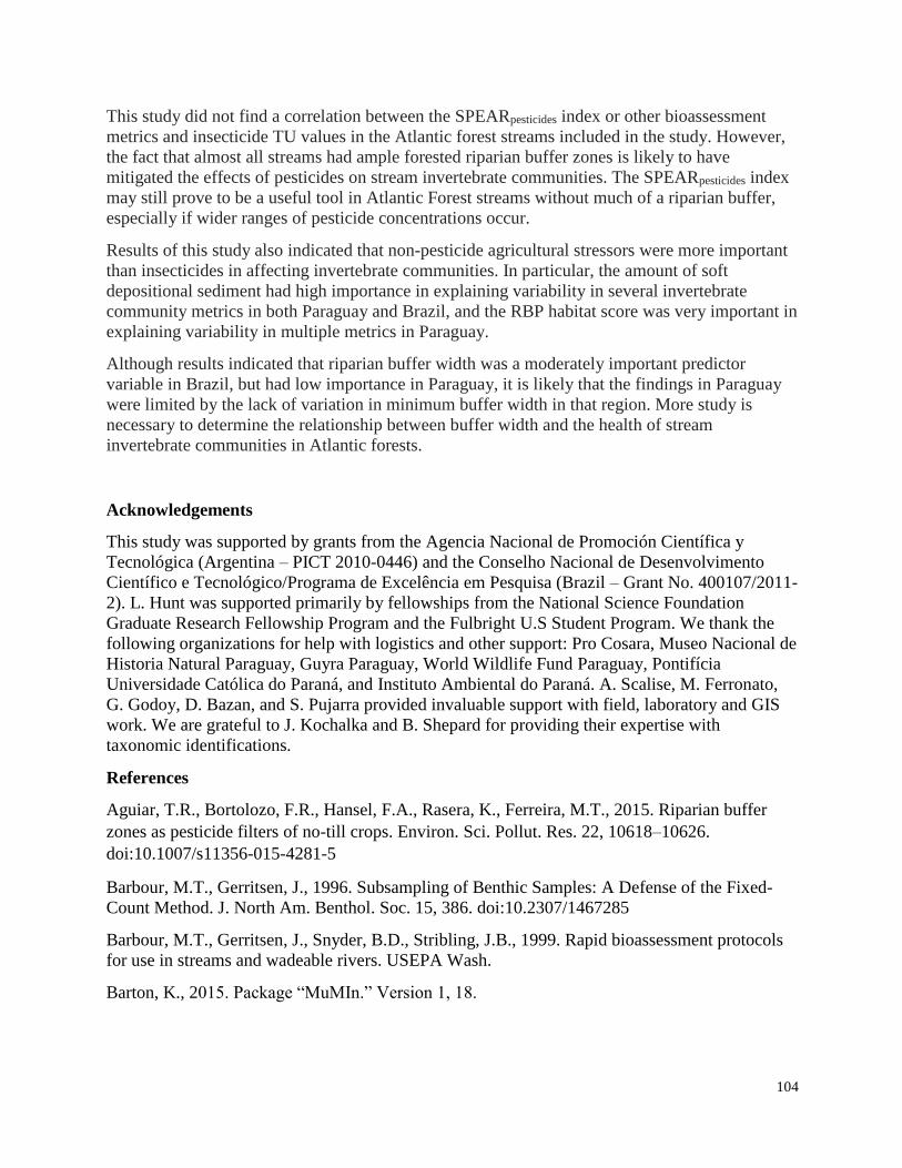
104
This study did not find a correlation between the SPEARpesticides index or other bioassessment
metrics and insecticide TU values in the Atlantic forest streams included in the study. However,
the fact that almost all streams had ample forested riparian buffer zones is likely to have
mitigated the effects of pesticides on stream invertebrate communities. The SPEARpesticides index
may still prove to be a useful tool in Atlantic Forest streams without much of a riparian buffer,
especially if wider ranges of pesticide concentrations occur.
Results of this study also indicated that non-pesticide agricultural stressors were more important
than insecticides in affecting invertebrate communities. In particular, the amount of soft
depositional sediment had high importance in explaining variability in several invertebrate
community metrics in both Paraguay and Brazil, and the RBP habitat score was very important in
explaining variability in multiple metrics in Paraguay.
Although results indicated that riparian buffer width was a moderately important predictor
variable in Brazil, but had low importance in Paraguay, it is likely that the findings in Paraguay
were limited by the lack of variation in minimum buffer width in that region. More study is
necessary to determine the relationship between buffer width and the health of stream
invertebrate communities in Atlantic forests.
Acknowledgements
This study was supported by grants from the Agencia Nacional de Promoción Científica y
Tecnológica (Argentina – PICT 2010-0446) and the Conselho Nacional de Desenvolvimento
Científico e Tecnológico/Programa de Excelência em Pesquisa (Brazil – Grant No. 400107/2011-
2). L. Hunt was supported primarily by fellowships from the National Science Foundation
Graduate Research Fellowship Program and the Fulbright U.S Student Program. We thank the
following organizations for help with logistics and other support: Pro Cosara, Museo Nacional de
Historia Natural Paraguay, Guyra Paraguay, World Wildlife Fund Paraguay, Pontifícia
Universidade Católica do Paraná, and Instituto Ambiental do Paraná. A. Scalise, M. Ferronato,
G. Godoy, D. Bazan, and S. Pujarra provided invaluable support with field, laboratory and GIS
work. We are grateful to J. Kochalka and B. Shepard for providing their expertise with
taxonomic identifications.
References
Aguiar, T.R., Bortolozo, F.R., Hansel, F.A., Rasera, K., Ferreira, M.T., 2015. Riparian buffer
zones as pesticide filters of no-till crops. Environ. Sci. Pollut. Res. 22, 10618–10626.
doi:10.1007/s11356-015-4281-5
Barbour, M.T., Gerritsen, J., 1996. Subsampling of Benthic Samples: A Defense of the Fixed-
Count Method. J. North Am. Benthol. Soc. 15, 386. doi:10.2307/1467285
Barbour, M.T., Gerritsen, J., Snyder, B.D., Stribling, J.B., 1999. Rapid bioassessment protocols
for use in streams and wadeable rivers. USEPA Wash.
Barton, K., 2015. Package “MuMIn.” Version 1, 18.
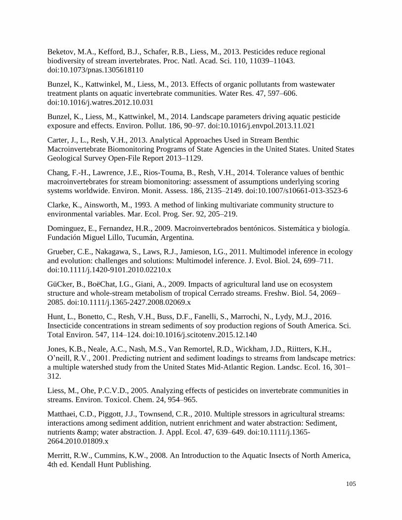
105
Beketov, M.A., Kefford, B.J., Schafer, R.B., Liess, M., 2013. Pesticides reduce regional
biodiversity of stream invertebrates. Proc. Natl. Acad. Sci. 110, 11039–11043.
doi:10.1073/pnas.1305618110
Bunzel, K., Kattwinkel, M., Liess, M., 2013. Effects of organic pollutants from wastewater
treatment plants on aquatic invertebrate communities. Water Res. 47, 597–606.
doi:10.1016/j.watres.2012.10.031
Bunzel, K., Liess, M., Kattwinkel, M., 2014. Landscape parameters driving aquatic pesticide
exposure and effects. Environ. Pollut. 186, 90–97. doi:10.1016/j.envpol.2013.11.021
Carter, J., L., Resh, V.H., 2013. Analytical Approaches Used in Stream Benthic
Macroinvertebrate Biomonitoring Programs of State Agencies in the United States. United States
Geological Survey Open-File Report 2013–1129.
Chang, F.-H., Lawrence, J.E., Rios-Touma, B., Resh, V.H., 2014. Tolerance values of benthic
macroinvertebrates for stream biomonitoring: assessment of assumptions underlying scoring
systems worldwide. Environ. Monit. Assess. 186, 2135–2149. doi:10.1007/s10661-013-3523-6
Clarke, K., Ainsworth, M., 1993. A method of linking multivariate community structure to
environmental variables. Mar. Ecol. Prog. Ser. 92, 205–219.
Dominguez, E., Fernandez, H.R., 2009. Macroinvertebrados bentónicos. Sistemática y biología.
Fundación Miguel Lillo, Tucumán, Argentina.
Grueber, C.E., Nakagawa, S., Laws, R.J., Jamieson, I.G., 2011. Multimodel inference in ecology
and evolution: challenges and solutions: Multimodel inference. J. Evol. Biol. 24, 699–711.
doi:10.1111/j.1420-9101.2010.02210.x
GüCker, B., BoëChat, I.G., Giani, A., 2009. Impacts of agricultural land use on ecosystem
structure and whole-stream metabolism of tropical Cerrado streams. Freshw. Biol. 54, 2069–
2085. doi:10.1111/j.1365-2427.2008.02069.x
Hunt, L., Bonetto, C., Resh, V.H., Buss, D.F., Fanelli, S., Marrochi, N., Lydy, M.J., 2016.
Insecticide concentrations in stream sediments of soy production regions of South America. Sci.
Total Environ. 547, 114–124. doi:10.1016/j.scitotenv.2015.12.140
Jones, K.B., Neale, A.C., Nash, M.S., Van Remortel, R.D., Wickham, J.D., Riitters, K.H.,
O’neill, R.V., 2001. Predicting nutrient and sediment loadings to streams from landscape metrics:
a multiple watershed study from the United States Mid-Atlantic Region. Landsc. Ecol. 16, 301–
312.
Liess, M., Ohe, P.C.V.D., 2005. Analyzing effects of pesticides on invertebrate communities in
streams. Environ. Toxicol. Chem. 24, 954–965.
Matthaei, C.D., Piggott, J.J., Townsend, C.R., 2010. Multiple stressors in agricultural streams:
interactions among sediment addition, nutrient enrichment and water abstraction: Sediment,
nutrients & water abstraction. J. Appl. Ecol. 47, 639–649. doi:10.1111/j.1365-
2664.2010.01809.x
Merritt, R.W., Cummins, K.W., 2008. An Introduction to the Aquatic Insects of North America,
4th ed. Kendall Hunt Publishing.
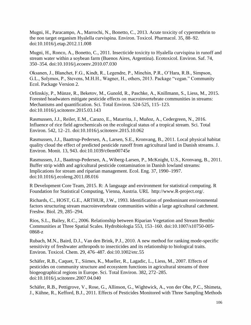
106
Mugni, H., Paracampo, A., Marrochi, N., Bonetto, C., 2013. Acute toxicity of cypermethrin to
the non target organism Hyalella curvispina. Environ. Toxicol. Pharmacol. 35, 88–92.
doi:10.1016/j.etap.2012.11.008
Mugni, H., Ronco, A., Bonetto, C., 2011. Insecticide toxicity to Hyalella curvispina in runoff and
stream water within a soybean farm (Buenos Aires, Argentina). Ecotoxicol. Environ. Saf. 74,
350–354. doi:10.1016/j.ecoenv.2010.07.030
Oksanen, J., Blanchet, F.G., Kindt, R., Legendre, P., Minchin, P.R., O’Hara, R.B., Simpson,
G.L., Solymos, P., Stevens, M.H.H., Wagner, H., others, 2013. Package “vegan.” Community
Ecol. Package Version 2.
Orlinskiy, P., Münze, R., Beketov, M., Gunold, R., Paschke, A., Knillmann, S., Liess, M., 2015.
Forested headwaters mitigate pesticide effects on macroinvertebrate communities in streams:
Mechanisms and quantification. Sci. Total Environ. 524-525, 115–123.
doi:10.1016/j.scitotenv.2015.03.143
Rasmussen, J.J., Reiler, E.M., Carazo, E., Matarrita, J., Muñoz, A., Cedergreen, N., 2016.
Influence of rice field agrochemicals on the ecological status of a tropical stream. Sci. Total
Environ. 542, 12–21. doi:10.1016/j.scitotenv.2015.10.062
Rasmussen, J.J., Baattrup-Pedersen, A., Larsen, S.E., Kronvang, B., 2011. Local physical habitat
quality cloud the effect of predicted pesticide runoff from agricultural land in Danish streams. J.
Environ. Monit. 13, 943. doi:10.1039/c0em00745e
Rasmussen, J.J., Baattrup-Pedersen, A., Wiberg-Larsen, P., McKnight, U.S., Kronvang, B., 2011.
Buffer strip width and agricultural pesticide contamination in Danish lowland streams:
Implications for stream and riparian management. Ecol. Eng. 37, 1990–1997.
doi:10.1016/j.ecoleng.2011.08.016
R Development Core Team, 2015. R: A language and environment for statistical computing. R
Foundation for Statistical Computing, Vienna, Austria. URL http://www.R-project.org/.
Richards, C., HOST, G.E., ARTHUR, J.W., 1993. Identification of predominant environmental
factors structuring stream macroinvertebrate communities within a large agricultural catchment.
Freshw. Biol. 29, 285–294.
Rios, S.L., Bailey, R.C., 2006. Relationship between Riparian Vegetation and Stream Benthic
Communities at Three Spatial Scales. Hydrobiologia 553, 153–160. doi:10.1007/s10750-005-
0868-z
Rubach, M.N., Baird, D.J., Van den Brink, P.J., 2010. A new method for ranking mode-specific
sensitivity of freshwater arthropods to insecticides and its relationship to biological traits.
Environ. Toxicol. Chem. 29, 476–487. doi:10.1002/etc.55
Schäfer, R.B., Caquet, T., Siimes, K., Mueller, R., Lagadic, L., Liess, M., 2007. Effects of
pesticides on community structure and ecosystem functions in agricultural streams of three
biogeographical regions in Europe. Sci. Total Environ. 382, 272–285.
doi:10.1016/j.scitotenv.2007.04.040
Schäfer, R.B., Pettigrove, V., Rose, G., Allinson, G., Wightwick, A., von der Ohe, P.C., Shimeta,
J., Kühne, R., Kefford, B.J., 2011. Effects of Pesticides Monitored with Three Sampling Methods

107
in 24 Sites on Macroinvertebrates and Microorganisms. Environ. Sci. Technol. 45, 1665–1672.
doi:10.1021/es103227q
Schäfer, R.B., von der Ohe, P.C., Rasmussen, J., Kefford, B.J., Beketov, M.A., Schulz, R., Liess,
M., 2012. Thresholds for the Effects of Pesticides on Invertebrate Communities and Leaf
Breakdown in Stream Ecosystems. Environ. Sci. Technol. 46, 5134–5142.
doi:10.1021/es2039882
Stehle, S., Schulz, R., 2015. Agricultural insecticides threaten surface waters at the global scale.
Proc. Natl. Acad. Sci. 112, 5750–5755. doi:10.1073/pnas.1500232112
Stone, M.L., Whiles, M.R., Webber, J.A., Williard, K.W.J., Reeve, J.D., 2005. Macroinvertebrate
Communities in Agriculturally Impacted Southern Illinois Streams. J. Environ. Qual. 34, 907.
doi:10.2134/jeq2004.0305
Whiles, M.R., Brock, B.L., Franzen, A.C., Dinsmore, II, S.C., 2000. Stream Invertebrate
Communities, Water Quality, and Land-Use Patterns in an Agricultural Drainage Basin of
Northeastern Nebraska, USA. Environ. Manage. 26, 563–576. doi:10.1007/s002670010113
Wood, P.J., Armitage, P.D., 1997. Biological effects of fine sediment in the lotic environment.
Environ. Manage. 21, 203–217.
You, J., Pehkonen, S., Weston, D.P., Lydy, M.J., 2008. Chemical availability and sediment
toxicity of pyrethroid insecticides to Hyalella azteca: Application to field sediment with
unexpectedly low toxicity. Environ. Toxicol. Chem. 27, 2124–2130.
You, J., Schuler, L.J., Lydy, M.J., 2004. Acute Toxicity of Sediment-Sorbed Endrin,
Methoxychlor, and Endosulfan to Hyalella azteca and Chironomus tentans. Bull. Environ.
Contam. Toxicol. 73. doi:10.1007/s00128-004-0451-8

108
Figure 1. Overview of study regions and soy production intensity in Brazil and Paraguay and sampling
locations on tributaries of Pirapó River in Itapua, Paraguay and San Francisco River in Parana, Brazil.
Figure 2. PCA ordination of water and sediment quality parameters for sampling sites in the two study regions
(Brazil and Paraguay), the high and low buffer width groups (b), and the high and low buffer width groups
within each region (c). For Paraguay sites that were sampled twice, parameter values were averaged.
(a)
Brazil Paraguay
(b)
Buffer < 50m
Buffer > 50m
(c)
Br Buffer < 50m
Br Buffer > 50m
Pa Buffer < 50m
Pa Buffer > 50m
(d) TotalTU
Conductivity
Turbidity
TOC
Fines
SoftSediment
(d)
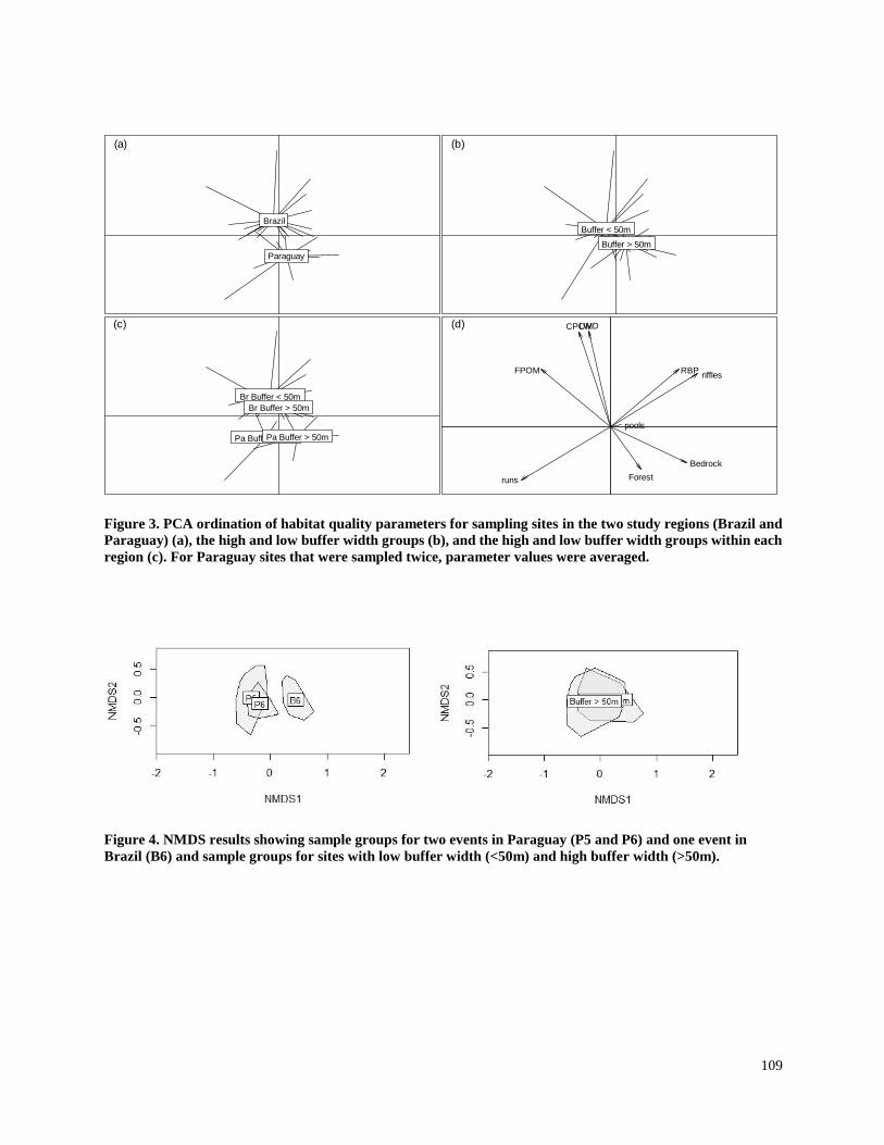
109
Figure 3. PCA ordination of habitat quality parameters for sampling sites in the two study regions (Brazil and
Paraguay) (a), the high and low buffer width groups (b), and the high and low buffer width groups within each
region (c). For Paraguay sites that were sampled twice, parameter values were averaged.
Figure 4. NMDS results showing sample groups for two events in Paraguay (P5 and P6) and one event in
Brazil (B6) and sample groups for sites with low buffer width (<50m) and high buffer width (>50m).
(a)
Brazil
Paraguay
(b)
Buffer < 50m
Buffer > 50m
(c)
Br Buffer < 50m
Br Buffer > 50m
Pa Buffer < 50m Pa Buffer > 50m
(d)
Bedrock
LWD
FPOM
CPOM
riffles
runs
pools
RBP
Forest
(d)
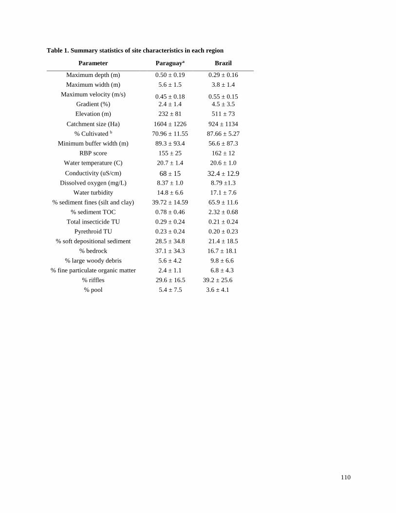
110
Table 1. Summary statistics of site characteristics in each region
Parameter Paraguaya Brazil
Maximum depth (m) 0.50 ± 0.19 0.29 ± 0.16
Maximum width (m) 5.6 ± 1.5 3.8 ± 1.4
Maximum velocity (m/s) 0.45 ± 0.18 0.55 ± 0.15
Gradient (%) 2.4 ± 1.4 4.5 ± 3.5
Elevation (m) 232 ± 81 511 ± 73
Catchment size (Ha) 1604 ± 1226 924 ± 1134
% Cultivated b 70.96 ± 11.55 87.66 ± 5.27
Minimum buffer width (m) 89.3 ± 93.4 56.6 ± 87.3
RBP score 155 ± 25 162 ± 12
Water temperature (C) 20.7 ± 1.4 20.6 ± 1.0
Conductivity (uS/cm) 68 ± 15 32.4 ± 12.9
Dissolved oxygen (mg/L) 8.37 ± 1.0 8.79 ±1.3
Water turbidity 14.8 ± 6.6 17.1 ± 7.6
% sediment fines (silt and clay) 39.72 ± 14.59 65.9 ± 11.6
% sediment TOC 0.78 ± 0.46 2.32 ± 0.68
Total insecticide TU 0.29 ± 0.24 0.21 ± 0.24
Pyrethroid TU 0.23 ± 0.24 0.20 ± 0.23
% soft depositional sediment 28.5 ± 34.8 21.4 ± 18.5
% bedrock 37.1 ± 34.3 16.7 ± 18.1
% large woody debris 5.6 ± 4.2 9.8 ± 6.6
% fine particulate organic matter 2.4 ± 1.1 6.8 ± 4.3
% riffles 29.6 ± 16.5 39.2 ± 25.6
% pool 5.4 ± 7.5 3.6 ± 4.1
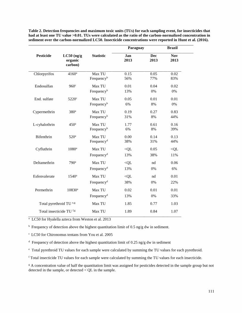
111
Table 2. Detection frequencies and maximum toxic units (TUs) for each sampling event, for insecticides that
had at least one TU value >0.01. TUs were calculated as the ratio of the carbon-normalized concentration in
sediment over the carbon-normalized LC50. Insecticide concentrations were reported in Hunt et al. (2016).
Paraguay Brazil
Pesticide LC50 (ng/g
organic
carbon)
Statistic Jan
2013
Dec
2013
Nov
2013
Chlorpyrifos 4160a Max TU 0.15 0.05 0.02
Frequencyb 56% 77% 83%
Endosulfan 960c Max TU 0.01 0.04 0.02
Frequencyb 13% 0% 0%
End. sulfate 5220c Max TU 0.05 0.01 0.01
Frequencyb 6% 8% 0%
Cypermethrin 380a Max TU 0.19 0.27 0.83
Frequencyb 31% 8% 44%
L-cyhalothrin 450a Max TU 1.77 0.61 0.16
Frequencyb 6% 8% 39%
Bifenthrin 520a Max TU 0.00 0.14 0.13
Frequencyd 38% 31% 44%
Cyfluthrin 1080a Max TU <QL 0.05 <QL
Frequencyd 13% 38% 11%
Deltamethrin 790a Max TU <QL nd 0.06
Frequencyd 13% 0% 6%
Esfenvalerate 1540a Max TU <QL nd 0.01
Frequencyd 38% 0% 22%
Permethrin 10830a Max TU 0.02 0.01 0.01
Frequencyd 13% 0% 33%
Total pyrethroid TU e,g Max TU 1.85 0.77 1.03
Total insecticide TU f,g Max TU 1.89 0.84 1.07
a LC50 for Hyalella azteca from Weston et al. 2013
b Frequency of detection above the highest quantitation limit of 0.5 ng/g dw in sediment.
c LC50 for Chironomus tentans from You et al. 2005
d Frequency of detection above the highest quantitation limit of 0.25 ng/g dw in sediment
e Total pyrethroid TU values for each sample were calculated by summing the TU values for each pyrethroid.
f Total insecticide TU values for each sample were calculated by summing the TU values for each insecticide.
g A concentration value of half the quantitation limit was assigned for pesticides detected in the sample group but not
detected in the sample, or detected < QL in the sample.
Table 3. Selected model results and relative importance of predictor variables included in averaged models. Includes only response metrics for which
significant correlations with predictor variables were found (p < 0.05), and models selected for averaging were those with and AIC<4. The coefficient
sign for each parameter is indicated after the relative importance value in brackets as (+) for positive correlation and (-) for negative correlation.
Parameters that are significantly correlated with response value (average p-value of selected models < 0.05) are indicated with an asterisk. Parameters
that are both significantly correlated and have moderated or high importance (>0.4) have values in bold.
11
2

Region Response
Metric
Selected
Models Relative Variable Importance
Adj.
r2 AICc
%
Agriculture
Buffer
width
Insecticide
TU RBP
%
Riffles Turbidity
Soft
sediment CPOM FPOM LWD TOC
Catchment
area Gradient
Brazil %EPT 0.34
to
0.79
147.8
to
151.7
0.62
(-)*
0.10
(+)
0.66
(-)
0.12
(-)*
0.17
(+)* 0.55 (-)* 0.40
(+)*
0.22
(-)
0.03
(-)
0.29 (-) 0.58(+)
%EPT-HB 0.51
to 0.63
125.3
to 129.0
0.07
(-) 0.51
(+)
0.62
(-)*
0.71
(-)*
0.06(+) 1.0
(+)*
% Ephem. 0.25
to
0.60
141.7
to
145.7
0.75
(-)*
0.59
(+)*
0.03(-) 0.45(-
)
0.04(-) 0.19(-) 0.32(+) 0.04(-) 0.10
(-)*
0.93
(+)*
% Trich. 0.17
to
0.45
98.1
to
102.0
0.20
(-)
0.07
(-)
0.05 (+) 0.05(-
)
0.14(-) 0.03(-) 0.83
(+)*
0.83
(-)*
0.04(-
)
0.03(+) 0.14(-) 0.03(-)
Coleop.
richness
0.18
to 0.52
41.1
to 45.0
0.03
(-)
0.14
(+)
0.19
(-)
0.03
(+)
0.38
(-) 0.80
(-)*
0.80
(+)*
0.18
(+)
0.39
(-)
Paraguay %EPT 0.78 to
0.88
119.5 to
121.8
0.76
(-)*
1.0
(+)*
1.0
(-)*
1.0
(-)*
1.0
(+)*
1.0
(+)*
%EPT-HB 0.27
to
0.50
119.5
to
123.5
0.39
(+)
0.07
(+)*
0.07
(-)*
0.42
(+) 0.93
(-)*
0.06
(+)
0.07
(-)*
0.43 (-) 0.17
(+)
% Ephem. 0.19
to 0.71
116.6
to 120.6
0.86
(+)*
0.67
(+)
0.34
(-)
0.21
(-)
0.19
(+)
0.09
(-)
0.15 (-) 0.20
(+)
0.30
(-)
% Trich. 0.19 to
0.49
111.0 to
114.9
0.02 (-)
0.18 (-)
0.14 (+)
0.46 (+)
0.72
(+)*
0.28 (-)
0.31 (+)
Adj.
r2 AICc
%
Agriculture
Buffer
width
Insecticide
TU RBP
%
Riffles Turbidity
Soft
sediment CPOM FPOM LWD TOC
Catchment
area Gradient
11
3

EPT
richness
0.28
to 0.54
56.1
to 59.7
0.66
(+) 0.89
(+)*
0.03
(-)
0.16
(-)
0.04
(-)
0.32
(-)
0.30
(-)
Trich. Richness
0.02 (+)
0.05 (-)
0.44 (+)
0.83
(+)*
0.06 (+)*
0.06 (+)
0.16 (-)
0.06 (+)
0.76
(-)*
0.07 (+)
0.14 (+)
0.02 (-)
Rare & Sensitive
0.40 to
0.74
47.0 to
51.0
1.0
(+)*
0.63
(-)*
1.0
(+)*
1.0
(-)*
0.38 (-)*
1.0
(-)*
Shannon
diversity
0.25
to
0.42
9.1 to
13.1
0.81
(+)*
0.06
(-)
0.19
(-)*
0.06
(-)
0.10
(-)
0.64
(-)*
Dominant
taxon
0.27
to 0.47
124.0
to 127.9
1.0 (-
)*
0.10
(-)
0.09
(+)
0.08
(+)
0.16
(-) 0.77
(+)*
3 dominant
taxa
0.28 to
0.43
119.0 to
123.6
0.04 (+)
0.04 (-)
0.05 (-)
0.23 (-)
0.05 (-)
0.04 (+)
0.86
(+)*
0.04 (+)
0.04 (-)
0.05 (+)
0.04 (+)
0.04 (-)
0.12 (+)
BMWP 0.34
to
0.69
141.3
to
145.2
0.02
(-)
0.05
(+) 1.0
(+)*
0.13
(-)
0.51
(-)
0.16
(+)
0.48
(+)
0.22
(+)
0.02
(+)
0.03
(-)
0.07
(-)*
ASPT 0.21
to 0.73
10.9
to 14.9
0.46
(-)
0.16
(+) 0.83
(+)*
0.62
(+)
0.12
(-)*
0.05
(-)
0.08
(+)*
0.06
(-)
0.19
(-)
0.13 (-) 0.01
(-)
0.27
(+)
SPEAR 0.56 to
0.75
92.0 to
96.0
0.14 (+)
0.13 (-)
0.71
(+)*
0.03 (+)
0.97
(+)*
0.41
(-)*
0.05 (+)
0.58 (-)
0.02 (-) 0.07 (+)
0.04 (-)
11
4

115
Table S1. Sampling Sites and Schedule
Site Name Latitude Longitude Jan
-13
Nov-
13
Dec
-13
BR-02 24 48 44.4S 53 42 31.6W X
BR-03 24 48 51.4S 53 38 22.2W X
BR-07 24 57 31.2S 53 40 53.5W X
BR-10 24 56 54.4S 53 41 52.5W X
BR-11 24 56 31.8S 53 42 49.1W X
BR-12 24 45 49.1S 53 48 55.7W X
BR-13 24 44 41.6S 53 51 40.3W X
BR-14 24 44 40.8S 53 51 59.3W X
BR-15 24 45 28.2S 53 52 55.8W X
BR-16 24 45 05.2S 53 53 03.6W X
BR-17 24 44 57.4S 53 54 18.2W X
BR-18 24 47 43.0S 53 54 11.0W X
BR-19 24 49 19.8S 53 54 12.2W X
BR-20 24 49 07.5S 53 50 29.2W X
BR-21 24 48 29.6S 53 45 44.8W X
BR-22 24 45 48.2S 53 37 54.1W X
BR-23 24 47 48.0S 53 36 16.8W X
BR-24 24 47 57.2S 53 36 01.7W X
SD 01 26 42 21.2S 55 31 49.1 W X X
SD 02 26 45 48.7S 55 33 34.7W X
SD 03 26 49 34.5S 55 31 36.8W X
SD 04 26 53 29.8S 55 34 19.1W X X
SD 05 26 55 54.1S 55 31 00.8W X X
SD 06 26 52 12.5S 55 29 49.7W X X
SD 07 26 37 45.8S 55 39 55.1W X X
SD 08 26 47 37.0S 55 37 33.4W X X
SD 09 26 47 59.4S 55 35 38.0W X X
SD 10 26 50 08.3S 55 36 33.2W X X
SD 11 26 50 35.0S 55 36 43.7W X
SD 12 26 31 29.1S 55 37 06.7W X
SD 13 26 32 18.4S 55 37 0.8W X X
SD 14 26 26 19.0S 55 34 32.4W X X
SD 15 26 30 56.5S 55 36 43.3W X
SD 16 26 28 21.9S 55 34 07.9W X X
SD 17 26 28 27.90S 55 33 57.40W X
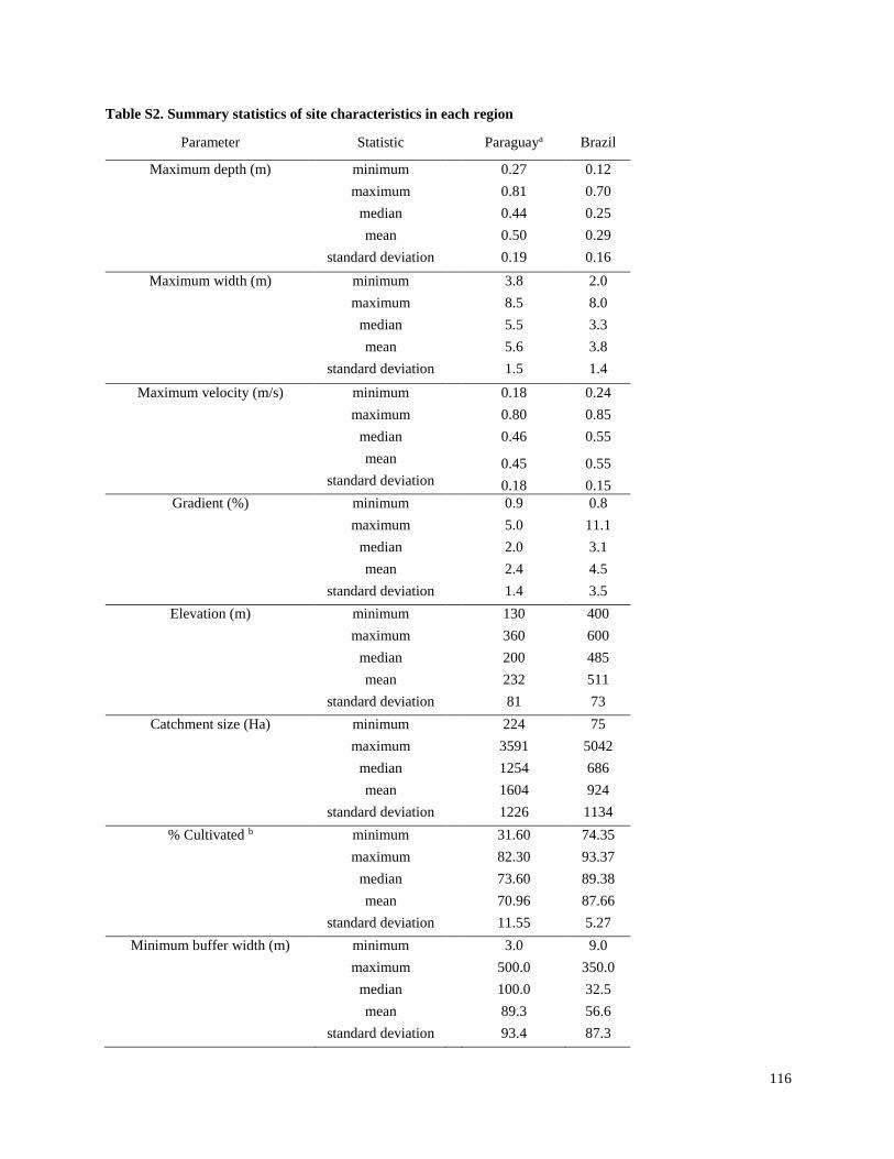
116
Table S2. Summary statistics of site characteristics in each region
Parameter Statistic Paraguaya Brazil
Maximum depth (m) minimum 0.27 0.12
maximum 0.81 0.70
median 0.44 0.25
mean 0.50 0.29
standard deviation 0.19 0.16
Maximum width (m) minimum 3.8 2.0
maximum 8.5 8.0
median 5.5 3.3
mean 5.6 3.8
standard deviation 1.5 1.4
Maximum velocity (m/s) minimum 0.18 0.24
maximum 0.80 0.85
median 0.46 0.55
mean 0.45 0.55
standard deviation 0.18 0.15
Gradient (%) minimum 0.9 0.8
maximum 5.0 11.1
median 2.0 3.1
mean 2.4 4.5
standard deviation 1.4 3.5
Elevation (m) minimum 130 400
maximum 360 600
median 200 485
mean 232 511
standard deviation 81 73
Catchment size (Ha) minimum 224 75
maximum 3591 5042
median 1254 686
mean 1604 924
standard deviation 1226 1134
% Cultivated b minimum 31.60 74.35
maximum 82.30 93.37
median 73.60 89.38
mean 70.96 87.66
standard deviation 11.55 5.27
Minimum buffer width (m) minimum 3.0 9.0
maximum 500.0 350.0
median 100.0 32.5
mean 89.3 56.6
standard deviation 93.4 87.3

117
RBP score minimum 79 134
maximum 182 180
median 162 164
mean 155 162
standard deviation 25 12
Water temperature (C) minimum 17.6 19.0
maximum 24.0 22.8
median 21.0 20.7
mean 20.7 20.6
standard deviation 1.4 1.0
Conductivity (uS/cm) minimum 34 14
maximum 91 60
median 70 30.5
mean 68 32.4
standard deviation 15 12.9
Dissolved oxygen (mg/L) minimum 2.90 7.30
maximum 10.00 14.60
median 8.42 8.50
mean 8.37 8.79
standard deviation 1.0 1.3
Water turbidity minimum 8.3 3.23
maximum 28.4 31
median 11.8 16.15
mean 14.8 17.1
standard deviation 6.6 7.6
% sediment fines (silt and clay) minimum 14.00 44.6
maximum 65.13 83.1
median 37.10 65.7
mean 39.72 65.9
standard deviation 14.59 11.6
% sediment TOC minimum 0.22 1.37
maximum 2.12 3.24
median 0.69 2.39
mean 0.78 2.32
standard deviation 0.46 0.68
Total insecticide TU minimum 0.07 0.03
maximum 1.01 1.07
median 0.20 0.14
mean 0.29 0.21
standard deviation 0.24 0.24
Pyrethroid TU minimum 0.04 0.03
maximum 0.98 1.03

118
aFor parameters that were measured during both sampling events in Paraguay, statistics are based on values that were
averaged over both sampling events.
bCultivated area was based on non-forested area, estimated with LANDSAT data.
median 0.15 0.13
mean 0.23 0.20
standard deviation 0.24 0.23
% soft depositional sediment minimum 0.0 0
maximum 100.0 70
median 7.5 17.5
mean 28.5 21.4
standard deviation 34.8 18.5
% bedrock minimum 0.0 0
maximum 95.0 50
median 35.0 10
mean 37.1 16.7
standard deviation 34.3 18.1
% large woody debris minimum 0.0 2
maximum 15.0 25
median 5.0 7.5
mean 5.6 9.8
standard deviation 4.2 6.6
% fine particulate organic matter minimum 2.0 2
maximum 5.0 20
median 2.0 5
mean 2.4 6.8
standard deviation 1.1 4.3
% riffles minimum 0.0 5
maximum 60.0 90
median 30.0 35
mean 29.6 39.2
standard deviation 16.5 25.6
% pool minimum 0.0 0
maximum 20.0 10
median 0.0 2.5
mean 5.4 3.6
standard deviation 7.5 4.1
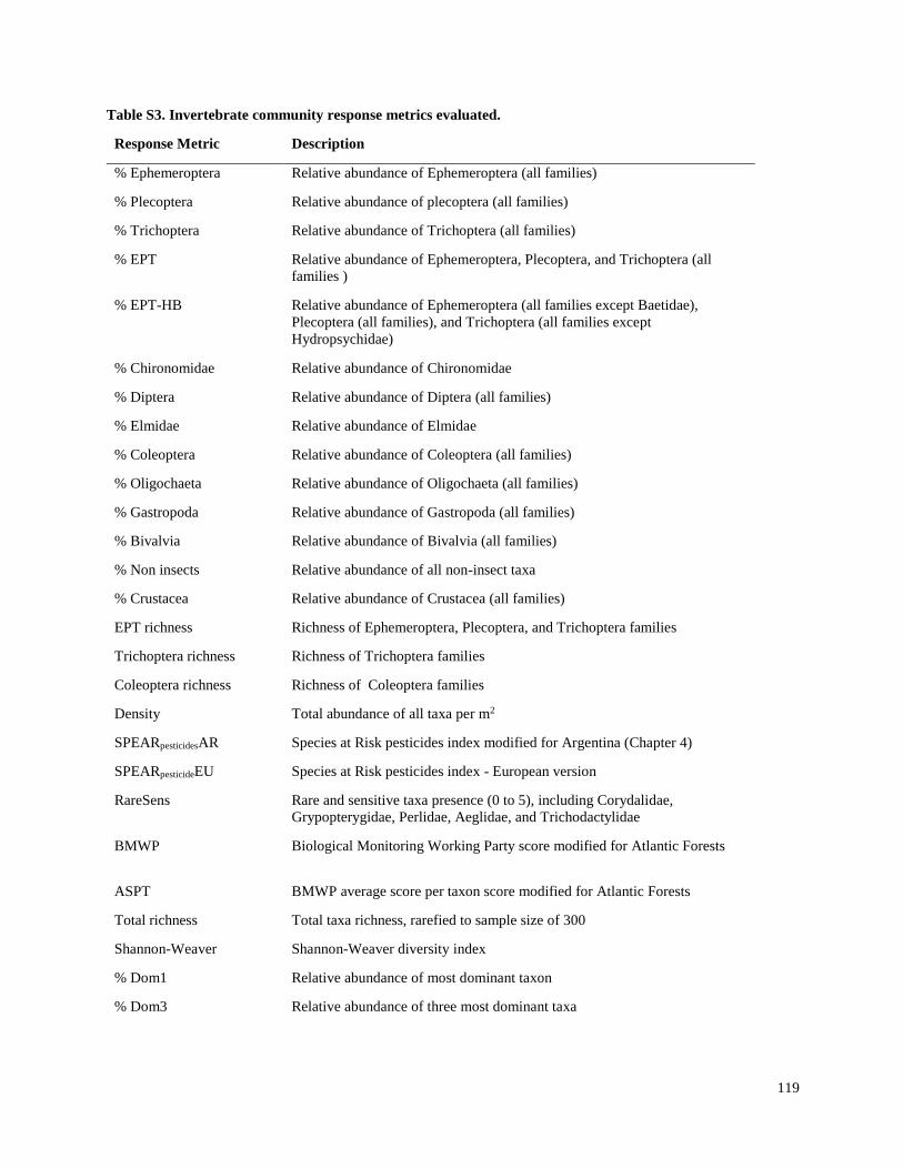
119
Table S3. Invertebrate community response metrics evaluated.
Response Metric Description
% Ephemeroptera Relative abundance of Ephemeroptera (all families)
% Plecoptera Relative abundance of plecoptera (all families)
% Trichoptera Relative abundance of Trichoptera (all families)
% EPT Relative abundance of Ephemeroptera, Plecoptera, and Trichoptera (all
families )
% EPT-HB Relative abundance of Ephemeroptera (all families except Baetidae),
Plecoptera (all families), and Trichoptera (all families except
Hydropsychidae)
% Chironomidae Relative abundance of Chironomidae
% Diptera Relative abundance of Diptera (all families)
% Elmidae Relative abundance of Elmidae
% Coleoptera Relative abundance of Coleoptera (all families)
% Oligochaeta Relative abundance of Oligochaeta (all families)
% Gastropoda Relative abundance of Gastropoda (all families)
% Bivalvia Relative abundance of Bivalvia (all families)
% Non insects Relative abundance of all non-insect taxa
% Crustacea Relative abundance of Crustacea (all families)
EPT richness Richness of Ephemeroptera, Plecoptera, and Trichoptera families
Trichoptera richness Richness of Trichoptera families
Coleoptera richness Richness of Coleoptera families
Density Total abundance of all taxa per m2
SPEARpesticidesAR Species at Risk pesticides index modified for Argentina (Chapter 4)
SPEARpesticideEU Species at Risk pesticides index - European version
RareSens Rare and sensitive taxa presence (0 to 5), including Corydalidae,
Grypopterygidae, Perlidae, Aeglidae, and Trichodactylidae
BMWP Biological Monitoring Working Party score modified for Atlantic Forests
ASPT BMWP average score per taxon score modified for Atlantic Forests
Total richness Total taxa richness, rarefied to sample size of 300
Shannon-Weaver Shannon-Weaver diversity index
% Dom1 Relative abundance of most dominant taxon
% Dom3 Relative abundance of three most dominant taxa

120
Table S4 Relative abundance and detection frequency of macroinvertebrate taxa and the Paraguay and Brazil
study streams
Paraguay Brazil
Relative
Abundance
(%)
%
Samples
detected
Relative
Abundance
(%)
%
Samples
detected
Coleoptera
Chrysomelidae 0.007 2.9 0.000 0.0
Dryopidae 0.026 2.9 0.023 11.1
Dytiscidae 0.013 2.9 0.023 11.1
Elmidae 21.200 97.1 12.457 100.0
Gyrinidae 0.007 2.9 0.011 5.6
Hydrophilidae 0.007 2.9 0.000 0.0
Lutrochidae 0.026 11.4 0.080 22.2
Psephenidae 0.765 57.1 0.616 50.0
Scarabaeidae 0.007 2.9 0.000 0.0
Diptera
Ceratopogonidae 0.310 48.6 0.856 83.3
Chironomidae 28.619 100.0 49.452 100.0
Empididae 0.053 17.1 2.407 100.0
Muscidae 0.007 2.9 0.034 11.1
Psychodidae 0.132 28.6 0.080 16.7
Simuliidae 1.576 65.7 3.034 94.4
Tabanidae 0.007 2.9 0.023 11.1
Tipulidae 0.264 34.3 0.422 66.7
Ephemeroptera
Baetidae 7.122 100.0 6.251 88.9
Caenidae 0.653 54.3 0.046 16.7
Leptohyphidae 12.443 100.0 0.068 22.2
Leptophlebiidae 1.879 88.6 7.506 88.9
Hemiptera
Belostomatidae 0.000 0.0 0.068 5.6
Corixidae 0.007 2.9 0.000 0.0
Gerridae 0.013 5.7 0.023 11.1
Helotrephidae 0.317 14.3 0.011 5.6
Mesoveliidae 0.007 2.9 0.000 0.0
Naucoridae 0.930 60.0 0.034 11.1
Pleidae 0.178 8.6 0.000 0.0
Veliidae 0.092 11.4 0.411 55.6
Lepidoptera
Crambidae 0.270 37.1 0.000 0.0
Megaloptera
Corydalidae 0.244 31.4 0.137 27.8
Odonata
Calopterygidae 0.185 8.6 0.068 27.8
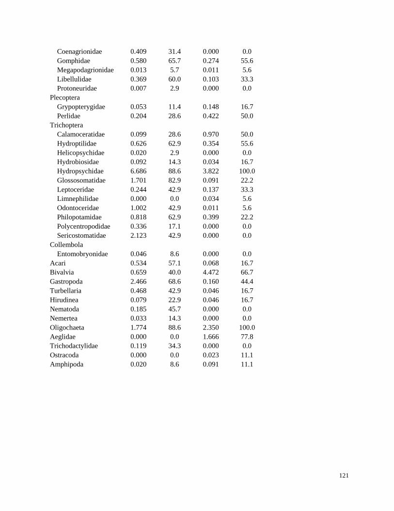
121
Coenagrionidae 0.409 31.4 0.000 0.0
Gomphidae 0.580 65.7 0.274 55.6
Megapodagrionidae 0.013 5.7 0.011 5.6
Libellulidae 0.369 60.0 0.103 33.3
Protoneuridae 0.007 2.9 0.000 0.0
Plecoptera
Grypopterygidae 0.053 11.4 0.148 16.7
Perlidae 0.204 28.6 0.422 50.0
Trichoptera
Calamoceratidae 0.099 28.6 0.970 50.0
Hydroptilidae 0.626 62.9 0.354 55.6
Helicopsychidae 0.020 2.9 0.000 0.0
Hydrobiosidae 0.092 14.3 0.034 16.7
Hydropsychidae 6.686 88.6 3.822 100.0
Glossosomatidae 1.701 82.9 0.091 22.2
Leptoceridae 0.244 42.9 0.137 33.3
Limnephilidae 0.000 0.0 0.034 5.6
Odontoceridae 1.002 42.9 0.011 5.6
Philopotamidae 0.818 62.9 0.399 22.2
Polycentropodidae 0.336 17.1 0.000 0.0
Sericostomatidae 2.123 42.9 0.000 0.0
Collembola
Entomobryonidae 0.046 8.6 0.000 0.0
Acari 0.534 57.1 0.068 16.7
Bivalvia 0.659 40.0 4.472 66.7
Gastropoda 2.466 68.6 0.160 44.4
Turbellaria 0.468 42.9 0.046 16.7
Hirudinea 0.079 22.9 0.046 16.7
Nematoda 0.185 45.7 0.000 0.0
Nemertea 0.033 14.3 0.000 0.0
Oligochaeta 1.774 88.6 2.350 100.0
Aeglidae 0.000 0.0 1.666 77.8
Trichodactylidae 0.119 34.3 0.000 0.0
Ostracoda 0.000 0.0 0.023 11.1
Amphipoda 0.020 8.6 0.091 11.1
122
CHAPTER 6
Conclusions and future directions
123
Conclusions and future directions
The results of my dissertation research demonstrated that: (1) there was consistency in the
insecticides that were most commonly detected in sediment samples from streams in the
intensive soy production regions studied in Argentina, Brazil and Paraguay; (2) these
insecticides, especially the pyrethroids, persisted in stream sediments at concentrations likely to
cause acute and chronic toxicity to aquatic invertebrates; and, (3) acutely toxic insecticide
concentrations in sediments were most likely to occur in streams with buffer widths less than
20m.
With respect to the impact of insecticides on stream invertebrate communities, results differed
between the Pampas study regions in Argentina and the Atlantic Forest regions in Brazil and
Paraguay. Chapter 4 demonstrated a correlation between insecticide toxic levels in stream
sediments and changes in aquatic invertebrate communities of the Argentine Pampas. The
SPEARpesticides index consistently showed a significant decrease with increasing insecticide TUs,
and insecticide TU was the most important variable in explaining variability in the SPEARpesticides
index, indicating that it is relatively insensitive to non-pesticide stressors. However, Chapter 5
showed that in the Paraguay and Brazil study regions there was no clear correlation between
insecticide toxic levels and SPEARpesticides or other invertebrate community metrics. Results
indicated that non-pesticide agricultural stressors were more important than insecticides in
affecting invertebrate communities. In particular, the amount of soft depositional sediment had
high importance in explaining variability in several invertebrate community metrics in both
Paraguay and Brazil, and the RBP habitat score was very important in explaining variability in
multiple metrics in Paraguay.
Crustaceans, especially amphipods in the genus Hyalella, comprised a large part of the stream
invertebrate communities in the Argentine Pampas, and also played an important role as sensitive
taxa in performance of the SPEARpesticides index in that region.Chapter 3 showed that the most
common native species of Hyalellais highly sensitive to the four insecticides most commonly
detected.Interestingly, amphipods were rare in Atlantic forest streams in Paraguay and Brazil,
likely because the habitat was unsuitable. The absence of these sensitive crustaceans may help
explain why the SPEARpesticides index did not perform well in streams of the Atlantic forest
regions. While some taxa in Atlantic forest streams may have similar sensitivity to pesticides as
amphipods, these other taxaare more likely to also be sensitive to many habitat and water quality
variables in addition to pesticides, potentially confounding the analysis. Amphipods are very
sensitive to pesticides but relatively tolerant of many habitat and water quality parameters
(Chapters 3 and 4). In contrast, other sensitive and abundant taxa (such as EPT taxa) tend to be
sensitive not only to pesticides but also to many habitat and water quality parameters (Bunzel et
al., 2013).When the SPEAR index threshold values were optimized for Argentine Pampas
streams, only the crustaceans and trichopterans were considered sensitive to pesticides, and
amphipods were the most abundant sensitive organisms, making them very important in the
performance of the SPEAR index. The role of Hyalella amphipods in Argentine streams
contrasts with the role of Gammarusamphipods in the SPEARpesticides index in Europe. Although
G. pulex has high physiological sensitivity to pesticides, this species can migrate very fast and
thus is considered not at risk to pesticides(Liess and Von der Ohe, 2005). I was unable to find
data on the migration rate of Hyalella species, but the decrease in relative abundance of
amphipods corresponding with increase in insecticide toxic units demonstrates that Hyalella
should be considered to have high overall sensitivity to insecticides.
124
The presence of forested riparian buffers along the entire lengths of all streams may also help
explain why SPEARpesticides index values were not significantly correlated with insecticide TU
values in either of the Atlantic forest regions. The forested riparian zones are likely to increase
the resilience and recovery ability of invertebrate communities. There is ample evidence that
forested headwaters provide reservoirs of invertebrate populations that assist in the recovery of
downstream communities after disturbance (Liess and Ohe, 2005; Orlinskiy et al., 2015). In
costrast, the stream buffers in Argentina were much smaller and were not forested, thus the
invertebrate communities may not have been as resilient.
It is also possible that the relative effects of buffer widths in protecting invertebrate communities
were less evident in my Atlantic Forest study than in other similar studies in which streams
generally had much smaller buffer width. Although there were some differences in relative buffer
width, all of the streams in both of my Atlantic Forest study regions can be considered well
protected in comparison to streams in many other intensive agricultural regions throughout the
world. In contrast, previous studies that have found riparian buffer zones to be effective in
mitigating effects on stream invertebrate communities have generally evaluated streams with
much smaller protected buffer zones than those considered in my study (Whiles et al. 2000;Rios
and Bailey, 2006). In my Brazil study area, where buffer widths were generally lower than those
in Paraguay, buffer width did have moderate importance in explaining variability in several
invertebrate metrics, while in Paraguay it had little or no importance.Although results indicated
that riparian buffer width was a moderately important predictor variable in Brazil, but had low
importance in Paraguay, it is likely that the findings in Paraguay were limited by the lack of
variation in minimum buffer width in that region. Approximately half of the Paraguay sites had
minimum buffer widths of 100m, which was the minimum required by law.
My study results corroborate findings from other studies that have found riparian buffer zones to
be important in mitigating transport of pesticides to streams. The present study’s finding of the
highest TU values in streams with buffer widths less than 20 m was within the range of buffer
widths (5 m to 20 m) reported to mitigate pesticide effects on streams (Rasmussen et al. 2011; Di
Marzio 2010; Bunzel et al. 2014; Reichenberger et al. 2007). Many factors could affect the buffer
width necessary to protect streams from pesticide exposure, including gradient, type of
vegetation, soil properties, types of pesticides applied, timing and amount of pesticides applied,
and presence of tile drains or drainage ditches that short-circuit the buffer zones (Reichenberger
et al. 2007; Bunzel et al. 2014). Although regulation of pesticide mitigation measures often
focuses on application practices, landscape level mitigation measures, such as requiring riparian
buffer zones, may be easier to implement and enforce. For example, Bereswill et al. (2014)
reviewed the efficacy and practicality of risk mitigation measures for diffuse pesticide entry into
aquatic ecosystems, and ranked riparian buffer strips as highly effective for mitigating both spray
drift and runoff, with high acceptability and feasibility. Riparian buffer zones are required to be
maintained in both Brazil and Paraguay, although specific requirements are in flux. However, the
implementation and enforcement of new riparian buffer requirements in Brazil has been difficult
and controversial, especially in regions with small-scale production where a significant amount
of a landowner’s productive farmland could be lost with compliance (Alvez et al. 2012). More
research is needed to determine the effectiveness of current and proposed riparian buffer
regulations in Paraguay and Brazil in protecting stream habitat, water quality, and ecosystems.
To my knowledge, the results I present in Chapter 4 constitute the first field study that has
demonstrated such effects of insecticides on invertebrate communities in soy production regions.
125
In intensive soy production regionsinthe midwest region of the United States,as well as in Brazil
and Argentina, many studies have reported frequent detections of insecticides, as well as toxicity
to specific sensitive species (Casara et al., 2012; Di Marzio et al., 2010; Ding et al., 2010; Hladik
and Kuivila, 2012; Jergentz et al., 2004a, 2004b; Laabs et al., 2002; Mugni et al., 2011).
However, none of these studies investigated effects on entire invertebrate communities over a
gradient of pesticide concentrations.
This research was the first application of the SPEAR index in South America, and the first to use
it to evaluate effects of pesticides on invertebrate communities associated with aquatic
vegetation. The SPEARpesticides index performed equally well for aquatic invertebrate
communities associated with emergent vegetation as it did for benthic invertebrate communities.
The results of my research are consistent with previous studies that have shown the
SPEARpesticides index to not be highly influenced by non-pesticide variables (Beketov and Liess,
2008; Liess et al., 2008a, 2008b). Although the SPEAR index was developed in Europe, it
performed well in the Argentine Pampas with only minor modifications, and would likely
improve as more data are obtained on South American taxa traits such as generation time and
migration rates.
This research did not find a correlation between the SPEARpesticides index and insecticide TU
values in the Atlantic forest streams included in the study. However, the fact that almost all
streams had ample forested riparian buffer zones is likely to have mitigated the effects of
pesticides on stream invertebrate communities. The SPEARpesticides index may still prove to be a
useful tool in Atlantic Forest streams without much of a riparian buffer, especially if wider
ranges of pesticide concentrations occur.
Chapters 3 and 4 contribute valuable information on pesticide sensitivity of an important South
American amphipod species with laboratory studies as well as field studies, and indicates that its
sensitivity is very similar to the closely related North America species H. azteca. A repeated
criticism is the lack of sensitivity data on species that occur outside of Europe and North
America, and there may be reason to believe that sensitivities could be different in species
occurring in the Southern hemisphere and near the equator. For example, Kwok et al. (2007)
found that tropical species may be more sensitive than temperate species to pesticides, while
temperate species are likely to be more sensitive to metals. More studies are needed on a range of
organisms to determine whether use of sensitivity data for northern hemisphere species are
adequately protective.
Although the neonicotinoid insecticides were not analyzed as part of the present study because
there was little evidence of their use at the start of field work, it is likely that their use in the soy
production in South America has increased in recent years, and will continue to increase. In
South America, neonicotinoids are often applied in combination with pyrethroids for control of
hemipteran pests in soy. In Argentina, there are at least 57 neonicotinoid/pyrethroid mixture
formulations registered for this purpose, although not all of them are currently in commercial use
(Servicio Nacional de Sanidad y Calidad Agroalimentaria, personal communication, Dec 2013).
Recent studies in soy production regions of South America detected imidacloprid in 43% of
surface water samples (Argentina; de Geronimo et al. 2014) and thiamethoxam in 100% of
surface water samples (Brazil; Rocha et al. 2015). A review of neonicotinoid studies around the
world found that 81% of the studies found maximum surface water concentrations that exceeded
an acute toxicity threshold, and 74% found average concentrations that exceeded a chronic

126
threshold (Morrissey et al. 2014). Future studies in soy production regions of South America
should include analysis of the occurrence and effects of neonicotinoids in aquatic ecosystems.
My results suggest that the following recommendations should be considered in soy production
regions of South America: (1) evaluation and implementation of buffer zones and other
management practices to limit transport of pesticides to streams; (2) field studies focusing on
effects to aquatic invertebrate communities; and, (3) continued monitoring that is adapted based
on quickly changing pesticide use trends.
References
Beketov, M.A., Liess, M., 2008. An indicator for effects of organic toxicants on lotic invertebrate
communities: Independence of confounding environmental factors over an extensive river
continuum. Environ. Pollut. 156, 980–987. doi:10.1016/j.envpol.2008.05.005
Bunzel, K., Kattwinkel, M., Liess, M., 2013. Effects of organic pollutants from wastewater
treatment plants on aquatic invertebrate communities. Water Res. 47, 597–606.
doi:10.1016/j.watres.2012.10.031
Casara, K.P., Vecchiato, A.B., Lourencetti, C., Pinto, A.A., Dores, E.F., 2012. Environmental
dynamics of pesticides in the drainage area of the São Lourenço River headwaters, Mato Grosso
State, Brazil. J. Braz. Chem. Soc. 23, 1719–1731.
Di Marzio, W.D., Sáenz, M.E., Alberdi, J.L., Fortunato, N., Cappello, V., Montivero, C.,
Ambrini, G., 2010. Environmental impact of insecticides applied on biotech soybean crops in
relation to the distance from aquatic ecosystems. Environ. Toxicol. Chem. n/a–n/a.
doi:10.1002/etc.246
Ding, Y., Harwood, A.D., Foslund, H.M., Lydy, M.J., 2010. Distribution and toxicity of
sediment-associated pesticides in urban and agricultural waterways from Illinois, USA. Environ.
Toxicol. Chem. 29, 149–157. doi:10.1002/etc.13
Hladik, M.L., Kuivila, K.M., 2012. Pyrethroid insecticides in bed sediments from urban and
agricultural streams across the United States. J. Environ. Monit. 14, 1838.
doi:10.1039/c2em10946h
Jergentz, S., Mugni, H., Bonetto, C., Schulz, R., 2004a. Runoff-Related Endosulfan
Contamination and Aquatic Macroinvertebrate Response in Rural Basins Near Buenos Aires,
Argentina. Arch. Environ. Contam. Toxicol. 46. doi:10.1007/s00244-003-2169-8
Jergentz, S., Pessacq, P., Mugni, H., Bonetto, C., Schulz, R., 2004b. Linking in situ bioassays
and population dynamics of macroinvertebrates to assess agricultural contamination in streams of
the Argentine pampa. Ecotoxicol. Environ. Saf. 59, 133–141. doi:10.1016/j.ecoenv.2004.06.007
Kwok, K.W., Leung, K.M., Lui, G.S., Chu, V.K., Lam, P.K., Morritt, D., Maltby, L., Brock, T.,
Van den Brink, P.J., Warne, M.S.J., others, 2007. Comparison of tropical and temperate
freshwater animal species’ acute sensitivities to chemicals: Implications for deriving safe
extrapolation factors. Integr. Environ. Assess. Manag. 3, 49–67.
Laabs, V., Amelung, W., Pinto, A.A., Wantzen, M., da Silva, C.J., Zech, W., 2002. Pesticides in
surface water, sediment, and rainfall of the northeastern Pantanal basin, Brazil. J. Environ. Qual.
31, 1636–1648.

127
Liess, M., Ohe, P.C.V.D., 2005. Analyzing effects of pesticides on invertebrate communities in
streams. Environ. Toxicol. Chem. 24, 954–965.
Liess, M., Schäfer, R.B., Schriever, C.A., 2008a. The footprint of pesticide stress in
communities—Species traits reveal community effects of toxicants. Sci. Total Environ. 406,
484–490. doi:10.1016/j.scitotenv.2008.05.054
Liess, M., Schäfer, R.B., Schriever, C.A., 2008b. The footprint of pesticide stress in
communities—Species traits reveal community effects of toxicants. Sci. Total Environ. 406,
484–490. doi:10.1016/j.scitotenv.2008.05.054
Liess, M., Von der Ohe, P.C.D., 2005. Analyzing effects of pesticides on invertebrate
communities in streams. Environ. Toxicol. Chem. 24, 954–965.
Mugni, H., Ronco, A., Bonetto, C., 2011. Insecticide toxicity to Hyalella curvispina in runoff and
stream water within a soybean farm (Buenos Aires, Argentina). Ecotoxicol. Environ. Saf. 74,
350–354. doi:10.1016/j.ecoenv.2010.07.030
Orlinskiy, P., Münze, R., Beketov, M., Gunold, R., Paschke, A., Knillmann, S., Liess, M., 2015.
Forested headwaters mitigate pesticide effects on macroinvertebrate communities in streams:
Mechanisms and quantification. Sci. Total Environ. 524-525, 115–123.
doi:10.1016/j.scitotenv.2015.03.143
Rios, S.L., Bailey, R.C., 2006. Relationship between Riparian Vegetation and Stream Benthic
Communities at Three Spatial Scales. Hydrobiologia 553, 153–160. doi:10.1007/s10750-005-
0868-z
Whiles, M.R., Brock, B.L., Franzen, A.C., Dinsmore, II, S.C., 2000. Stream Invertebrate
Communities, Water Quality, and Land-Use Patterns in an Agricultural Drainage Basin of
Northeastern Nebraska, USA. Environ. Manage. 26, 563–576. doi:10.1007/s002670010113