Effects of Inlet Geometry on Hydraulic Performance of …sddot.com/business/research/projects/docs/SD2002_04_Final_Report.pdfDesign coefficients are recommended for several ... Effects

Publication No. FHWA-RD-04-138 December 2004

Effects of Inlet Geometry on Hydraulic Performance of Box Culverts Laboratory Report

U.S. DEPARTMENT OF TRANSPORTATION

Federal Highway Administration

Research and Development Turner-Fairbank Highway Research Center 6300 Georgetown Pike McLean, VA 22101-2296

C onnecting South D akota and the N ation

FOREWORD This report describes a laboratory study of culvert hydraulics done at the TFHRC hydraulics lab in partnership with the South Dakota DOT (SD DOT). The study focused on rectangular shaped culverts with a number of inlet geometry conditions representing inlets that are currently available for highway culverts. Design coefficients are recommended for several inlet configurations that are not specifically covered in the Federal Highway Administration Hydraulic Design Series No. 5 (HDS-5). This report will be of interest to hydraulic engineers involved in culvert design and to researchers involved in developing improved culvert design guidelines. It is being published as a Web document only.

Gary Henderson.

Director, Office of Infrastructure

Research and Development

Notice This document is disseminated under the sponsorship of the U.S. Department of Transportation in the interest of information exchange. The U.S. Government assumes no liability for the use of the information contained in this document. This report does not constitute a standard, specification, or regulation.

The U.S. Government does not endorse products or manufacturers. Trademarks or manufacturers' names appear in this report only because they are considered essential to the objective of the document.

Quality Assurance Statement The Federal Highway Administration (FHWA) provides high-quality information to serve Government, industry, and the public in a manner that promotes public understanding. Standards and policies are used to ensure and maximize the quality, objectivity, utility, and integrity of its information. FHWA periodically reviews quality issues and adjusts its programs and processes to ensure continuous quality improvement.

DISCLAIMER

The contents of this report reflect the views of the authors who are responsible for the facts and accuracy of the data presented herein. The contents do not necessarily reflect the official views or policies of the South Dakota Department of Transportation, the State Transportation Commission, or the Federal Highway Administration. This report does not constitute a standard, specification, or regulation.

ACKNOWLEDGEMENTS

This work was performed under the supervision of the SD2002-04 Technical Panel: Mark Clausen ................................................ FHWA Noel Clocksin....................................................LGA Kevin Goeden.....................Office of Bridge Design Corey Haeder .......South Dakota Concrete Products Terry Jorgensen................................................ LGA Paul Oien .................................................... Research Daris Ormesher ...........................Office of Research Rich Phillips .......................Office of Bridge Design Steve Wagner ......................................South Dakota The work was performed in cooperation with the United States Department of Transportation Federal Highway Administration.

ii

(This page intentionally left blank)

iii

1. Report No 2. Government Accession No. 3. Recipient's Catalog No.

FHWA-RD-04-138 N/A N/A

4. Title and Subtitle 5. Report Date

6. Performing Organization Code

Effects of Inlet Geometry on Hydraulic Performance of Box Culverts

N/A

7. Authors(s) 8. Performing Organization Report No.

J. Sterling Jones, Kornel Kerenyi, and Stuart Stein N/A

9. Performing Organization Name and Address 10. Work Unit No. (TRAIS)

N/A

11. Contract or Grant No.

DTFH61—04-C-00037

13. Type of Report and Period Covered

GKY and Associates, Inc. 5411-E Backlick Road Springfield, VA 22151

Final Lab Report 11-02 to 11-04

12. Sponsoring Agency Name and Address 14. Sponsoring Agency Code

Office of Infrastructure R&D South Dakota DOT Federal Highway Administration Office of Research 6300 Georgetown Pike 700 E. Broadway Avenue McLean, VA 22101 Pierre, SD 57501

SD Project SD2002-04 FHWA Task Order 3

15. Supplementary Notes

Contracting Officer’s Technical Representative: J. Sterling Jones South Dakota Technical Panel: Mark Clausen, Noel Clocksin, Kevin Goeden, Cory Haeder, Terry Jorgensen, Paul Oien, Daris Ormesher, Rich Phillips, Steve Wagner Brad Newlin designed models and developed preliminary analysis algorithms. Holger Dauster and Amon Tarakemeh provided invaluable assistance with instrumentation, data collection and analysis. Donna and Dave Pearson provided senior editing and EDP services.

16. Abstract

Each year the South Dakota Department of Transportation (SD DOT) designs and builds many cast-in-place (CIP) and precast box culvert structures that allow drainage to pass under roadways. The CIP boxes typically have 30-degree flared wing walls and the precast have straight wing walls with 4-in bevel on the inside edges of the wing walls and top slab. Previous research, SD93-12, conducted on a limited number of single barrel box culverts, indicated that further research was necessary to determine the effects of multiple barrel structures, loss coefficients of unsubmerged outlets, and to determine the effect of 12-in corner fillets versus 6-in corner fillets. In order to optimize the design of both types of box culverts, it was also necessary to determine the effects of span-to-rise ratio, skewed end condition, and optimum edge condition on typical box culvert installations

17. Key Words 18. Distribution Statement

No restrictions. This document is available to the public through the National Technical Information Service; Springfield, VA 22161

19. Security Classif. (of this report) 20. Security Classif. (of this page) 21. No. of Pages 22. Price

Unclassified Unclassified 180 N/A

Form DOT F 1700.7 (8-72) Reproduction of completed page authorized (art. 5/94)

iv

SI* (MODERN METRIC) CONVERSION FACTORS APPROXIMATE CONVERSIONS TO SI UNITS

Symbol When You Know Multiply By To Find Symbol LENGTH

in inches 25.4 millimeters mm ft feet 0.305 meters m yd yards 0.914 meters m mi miles 1.61 kilometers km

AREA in2 square inches 645.2 square millimeters mm2

ft2 square feet 0.093 square meters m2

yd2 square yard 0.836 square meters m2

ac acres 0.405 hectares ha mi2 square miles 2.59 square kilometers km2

VOLUME fl oz fluid ounces 29.57 milliliters mL gal gallons 3.785 liters L ft3 cubic feet 0.028 cubic meters m3

yd3 cubic yards 0.765 cubic meters m3

NOTE: volumes greater than 1000 L shall be shown in m3

MASS oz ounces 28.35 grams glb pounds 0.454 kilograms kgT short tons (2000 lb) 0.907 megagrams (or "metric ton") Mg (or "t")

TEMPERATURE (exact degrees) oF Fahrenheit 5 (F-32)/9 Celsius oC

or (F-32)/1.8 ILLUMINATION

fc foot-candles 10.76 lux lx fl foot-Lamberts 3.426 candela/m2 cd/m2

FORCE and PRESSURE or STRESS lbf poundforce 4.45 newtons N lbf/in2 poundforce per square inch 6.89 kilopascals kPa

APPROXIMATE CONVERSIONS FROM SI UNITS Symbol When You Know Multiply By To Find Symbol

LENGTHmm millimeters 0.039 inches in m meters 3.28 feet ft m meters 1.09 yards yd km kilometers 0.621 miles mi

AREA mm2 square millimeters 0.0016 square inches in2

m2 square meters 10.764 square feet ft2

m2 square meters 1.195 square yards yd2

ha hectares 2.47 acres ac km2 square kilometers 0.386 square miles mi2

VOLUME mL milliliters 0.034 fluid ounces fl oz L liters 0.264 gallons gal m3 cubic meters 35.314 cubic feet ft3

m3 cubic meters 1.307 cubic yards yd3

MASS g grams 0.035 ounces ozkg kilograms 2.202 pounds lbMg (or "t") megagrams (or "metric ton") 1.103 short tons (2000 lb) T

TEMPERATURE (exact degrees) oC Celsius 1.8C+32 Fahrenheit oF

ILLUMINATION lx lux 0.0929 foot-candles fc cd/m2 candela/m2 0.2919 foot-Lamberts fl

FORCE and PRESSURE or STRESS N newtons 0.225 poundforce lbf kPa kilopascals 0.145 poundforce per square inch lbf/in2

*SI is the symbol for th International System of Units. Appropriate rounding should be made to comply with Section 4 of ASTM E380. e(Revised March 2003)

v

TABLE OF CONTENTS

Page 1. EXECUTIVE SUMMARY ......................................................................... 1 FINDINGS AND CONCLUSIONS .................................................................... 1 RECOMMENDATIONS..................................................................................... 3 2. PROJECT DESCRIPTION........................................................................ 9 PROBLEM STATEMENT ................................................................................. 9 BACKGROUND SUMMARY .......................................................................... 10 OBJECTIVES .................................................................................................... 10 RESEARCH PLAN ........................................................................................... 10 PRODUCTS........................................................................................................ 15 IMPLEMENTATION ....................................................................................... 15 BENEFITS.......................................................................................................... 15 TIME SCHEDULE ............................................................................................ 15 STAFFING ......................................................................................................... 16 FACILITIES ...................................................................................................... 16 3. LITERATURE REVIEW .......................................................................... 19 4. THEORY AND DESIGN CALCULATIONS FOR INLET AND

OUTLET CONTROL ................................................................................ 25 INLET-CONTROL HYDRAULICS OF CULVERTS .................................. 25 OUTLET CONTROL HYDRAULICS OF CULVERTS .............................. 26 5. DATA ACQUISITION AND DATA ANALYSIS PROCEDURES ...... 29 DATA ACQUISITION FOR CULVERT SET-UP......................................... 29 DATA MANAGEMENT ................................................................................... 29 DATA ANALYSIS FOR INLET CONTROL TESTS ................................... 31 DATA ANALYSIS FOR OUTLET CONTROL TESTS ............................... 32 6. EXPERIMENTAL PROCEDURES ......................................................... 35 MINI-FLUME EXPERIMENTS...................................................................... 35 PIV – post processing............................................................................. 36 CULVERT SET-UP EXPERIMENTS ............................................................ 38 Inlet and culvert barrel models ............................................................ 41 7. EXPERIMENTAL RESULTS .................................................................. 43 EFFECTS OF BEVELS AND CORNER FILLETS ...................................... 43 Mini-flume test results for bevel effects ............................................... 43 Head loss experiments for bevel effects ............................................... 43 Effect of wing-wall-top-edge bevel ....................................................... 48 Effect of corner fillets ............................................................................ 49 EFFECTS OF MULTIPLE BARRELS........................................................... 53 Multiple barrels vs. single barrel.......................................................... 55 Effect of wing-wall-flare angle .............................................................. 57 Effect of center-wall extension .............................................................. 60 EFFECTS OF SPAN-TO-RISE RATIO.......................................................... 64 Multiple span to rise vs. basic 1:1 span to rise .................................... 64

vi

Effect of wing-wall flare related to span-to-rise ratio......................... 66 EFFECTS OF HEADWALL SKEW ............................................................... 71 OUTLET CONTROL ENTRANCE-LOSS COEFFICIENTS Ke FOR LOW FLOWS (UNSUBMERGED CONDITIONS) ...................................... 74 Effects of Reynolds number on Ke........................................................ 74 OUTLET CONTROL EXIT-LOSS COEFFICIENTS, Ko ............................ 78 FIFTH-ORDER POLYNOMIALS .................................................................. 83 8. CONCLUSIONS AND RECOMMENDATIONS ................................... 87 FINDINGS AND CONCLUSIONS .................................................................. 87 RECOMMENDATIONS................................................................................... 89 APPENDIX A. EXPANDED TEST MATRIX................................................ 103 APPENDIX B. INLET-CONTROL COMPARISON CHARTS .................. 113 APPENDIX C. SUMMARY OF REGRESSION COEFFICIENTS FOR ALL

EXPERIMENTS ....................................................................................... 133 APPENDIX D. EXAMPLE PROBLEM.......................................................... 147 APPENDIX E. REFERENCES .................................................................................... 165

vii

LIST OF TABLES

Table No. Page 1. Executive summary list of design coefficients suggested for implementation.................. 5 2. Summary of inlet and outlet control coefficients for models tested for effects of

bevel and corner fillets..................................................................................................... 52 3. Summary of inlet and outlet control coefficients for models tested for effects of

multiple barrels ................................................................................................................ 56 4. Summary of inlet and outlet control coefficients for models tested for effects of

span-to-rise ratio .............................................................................................................. 68 5. Summary of inlet and outlet control coefficients for models tested for effects of

skewed headwall .............................................................................................................. 73 6. Summary of outlet control entrance-loss coefficients, Ke for low flows......................... 75 7. Summary of outlet loss coefficients................................................................................. 82 8. Summary of polynomial regression coefficients for models tested for effects of

bevels and corner fillets ................................................................................................... 84 9. Summary of polynomial regression coefficients for models tested for effects of

span-to-rise ratio .............................................................................................................. 84 10. Summary of polynomial regression coefficients for models tested for effects of

multiple barrels ................................................................................................................ 85 11. Summary of polynomial regression coefficients for models tested for effects of

skewed headwall .............................................................................................................. 85 12. Design coefficients suggested for future editions of HDS-5 ........................................... 96 13. Fifth-order-polynomial coefficients................................................................................. 97 14. Task 6.1 tests performed in the culvert test facility to analyze the effects of

bevels for wing walls and top edge................................................................................ 105 15. Task 6.2 tests performed to analyze the effects of multiple barrels............................... 107 16. Task 6.3 tests performed to analyze the effects of span-to-rise ratio............................. 109 17. Task 6.4 tests performed to analyze the effects of skew................................................ 111 18. Summary of inlet-control design coefficients: all experiments ..................................... 135 19. Summary of inlet-control fifth-order polynomial coefficients; all experiments............ 137 20. Summary of outlet-control design coefficients; all experiments ................................... 141 21. Results from step backwater and entrance loss computations for Q25........................... 157 22. Results from step backwater and entrance loss computations for Q100 ......................... 158

viii


ix

LIST OF FIGURES

Figure No. Page 1. Thumbnail sketches of inlets recommended for implementation ...................................... 6 2. Culvert headbox under construction ................................................................................ 16 3. Arrangement of the ceramic class pressure sensors......................................................... 17 4. Experimental set up for Particle Image Velocimetry....................................................... 17 5. Sketch of precast-flared-end section tested by Graziano and by McEnroe ..................... 22 6. Conceptual sketch of entrance-loss coefficient related to Reynolds number

(Tullis, 2004).................................................................................................................... 24 7. Typical inlet-control-flow condition................................................................................ 25 8. Outlet control for full- flow condition ............................................................................. 27 9. Data management chart.................................................................................................... 30 10. Technique to determine HLe............................................................................................. 33 11. Typical behavior of Ke vs discharge intensity ................................................................. 33 12. Mini-flume and PIV set-up .............................................................................................. 35 13. Bevel models and PIV camera at culvert entrance .......................................................... 36 14. Tested bevel-edge conditions and effective flow-depth criterion.................................... 37 15. Integration of the velocity flow field results in stream functions to study flow

contraction in the culvert ................................................................................................. 38 16. Culvert set-up – side view................................................................................................ 39 17. Culvert set-up – top view................................................................................................. 39 18. Culvert set-up – over view............................................................................................... 40 19. Culvert model barrels....................................................................................................... 40 20. 2-D robot to measure velocity distribution in tailbox...................................................... 41 21. Groove connectors to assemble models........................................................................... 42 22. Effective flow depth at vena contracta for non-rounded bevel edges.............................. 44 23. Effective flow depth at vena contracta for rounded bevel edges ..................................... 45 24. Effective flow depth vs. headwater/tailwater difference ................................................. 46 25. Inlet-control performance curves FC-S-0 vs. PC-A with zero corner fillets ................... 46 26. Inlet-control performance curves FC-S-0 vs. PC-A with 6-in corner fillets.................... 47 27. Inlet-control: precast with 6-in fillets compared to field cast with 6-in fillets. ............... 47 28. Inlet-control: field-cast single inlet compared to a field-cast hybrid inlet with

4-in radius bevel on side walls......................................................................................... 48 29. Inlet-control: precast-single inlet compared to a precast-hybrid inlet with no

bevel on side walls. .......................................................................................................... 49 30. Inlet-control effects of corner fillets for the field-cast model.......................................... 50 31. Inlet-control effects of corner fillets for the precast model ............................................. 50 32. Inlet control: precast with 12-in fillets compared to field cast with 6-in fillets............... 51 33. Models tested for effects of bevels and corner fillets ...................................................... 53 34. Inlet control: comparison FC-S-0 inlet, FC-D-0 inlet, FC-T-0 inlet and FC-Q-0 inlet ... 54 35. Inlet control: comparison FC-S-30 inlet, FC-D-30 inlet, FC-T-30 inlet and

FC-Q-30 inlet ................................................................................................................... 55 36. Inlet control: comparison PC-A inlet, PC-B inlet, PC-C inlet and PC-D inlet................ 55

x

LIST OF FIGURES (CONT’D)

Figure No. Page 37. Inlet control: comparison FC-S-0 and FC-S-30 inlets and PC-A inlet ............................ 58 38. Inlet control: comparison FC-D-0 and FC-D-30 inlets and PC-B inlet ........................... 58 39. Inlet control: comparison FC-T-0 and FC-T-30 inlets and PC-C inlet............................ 59 40. Inlet control: comparison FC-Q-0 and FC-Q-30 inlets and PC-D inlet........................... 59 41. Inlet control: comparison FC-D-30 and FC-D-30-E inlets .............................................. 60 42. Inlet control: comparison PC-B and PC-B-E inlets ......................................................... 61 43. Models tested for effects of multiple barrels ................................................................... 63 44. Inlet control: comparison of different span-to-rise FC-S-0 inlets.................................... 64 45. Inlet control: comparison of different span-to-rise PC-A inlets ...................................... 65 46. Inlet control: comparison of different span-to-rise FC-S-30 inlets.................................. 65 47. Inlet control: comparison FC-S-0, FC-S-30 inlets and PC-A inlet (span to rise 1:1)...... 66 48. Inlet control: comparison FC-S-0, FC-S-30 inlets and PC-A inlet (span to rise 2:1)...... 67 49. Inlet control: comparison FC-S-0, FC-S-30 inlets and PC-A inlet (span to rise 3:1)...... 67 50. Inlet control: comparison FC-S-0, FC-S-30 inlets and PC-A inlet (span to rise 4:1)...... 68 51. Models tested for effects of span-to-rise ratio ................................................................. 70 52. Definition sketch for skew tests....................................................................................... 71 53. Comparing HDS-5 12/3 inlet with a FC-T-30 inlet for 0-degree, 15-degree,

3-degree, and 45-degree skew angles .............................................................................. 72 54. Models tested for effects of headwall skew: 15 degree, 30 degree, and 45 degree ........ 72 55. Plan view of skewed headwall models as tested.............................................................. 73 56. Entrance-loss coefficient for the HDX-5 8/3-inlet for different Reynolds numbers ....... 76 57. Standard deviation of the Ke data versus different Reynolds numbers including

a best-fit trend line ........................................................................................................... 77 58. Culvert contraction........................................................................................................... 78 59. Flow expansion in the tailbox for high tail water ............................................................ 80 60. Flow expansion in the tailbox for low tail water ............................................................. 80 61. Vertical flow expansion in the tailbox and projected EGL.............................................. 81 62. Transition between unsubmerged and submerged inlet data control flow conditions..... 83 63. Combined corner fillet data for field-cast models with the 45-degree-straight-top-plate

bevel and precast models with the 8-in-radius-top-plate bevel (sketches 7, 14 and 10 , 11 in figure 73)...................................................................................................................... 90

64. Combined multiple-barrel data for field-cast models with 0-degree-wing-wall flare (sketches 7 and 8 in figure 73)......................................................................................... 91

65. Combined multiple-barrel data for field-cast models with 30-degree-wing-wall flare (sketches 1 and 2 in figure 73)......................................................................................... 91

66. Combined multiple-barrel data for precast models with 0-degree-wing-wall flare (sketches 11 and 12 in figure 73)..................................................................................... 92

67. Combined span-to-loss data for field-cast models with 0-degree-wing-wall flare (sketches 7 and 9 in figure 73)......................................................................................... 92

68. Combined span-to-rise data for field-cast models with 0-degree-wing-wall flare (sketches 1 and 3 in figure 73)......................................................................................... 93

xi


Figure No. Page 69. Combined span-to-rise data for precast models with 0-degree-wing-wall flare

(sketches 10 and 13 in figure 73)..................................................................................... 93 70. Skewed headwalls at 15-degree, 30-degree, and 45-degree skews compared to

0-degree skew for triple-barrel-field-cast models with flared-wing walls (sketches 4 and 5 in figure 73)......................................................................................... 94

71. Precast single-barrel model compared to field-cast models (sketches 1, 7, and 11 in figure 73).......................................................................................................................... 94

72. Precast multiple-barrel models compared to field-cast models (sketches 7, 8, 1, 2, and 11, 12 in figure 73).................................................................................................... 95

73. Thumbnail sketches of inlets recommended for implementation .................................... 99 74. Edge configurations tested in the mini-flume................................................................ 104 75. Streamlines from particle imaging velocimetry experiments used to quantify effective

flow depths at vena contracta......................................................................................... 104 76. Inlet control: comparison FC-S-0 inlet and PC-A inlet ................................................. 113 77. Inlet control: comparison FC-S-0 inlet and PC-A inlet ................................................. 114 78. Inlet control: comparison FC-S-0 inlet and PC-A inlet ................................................. 114 79. Inlet control: comparison FC-S-30 and FC-S-0 inlets and PC-A inlet .......................... 115 80. Inlet control: comparison PC-A inlets ........................................................................... 115 81. Inlet control: field-cast-single inlet compared to a field-cast-hybrid inlet with

4-in-radius bevel on side walls ...................................................................................... 116 82. Inlet control: precast-single inlet compared to a precast-hybrid inlet with no bevel

on side walls................................................................................................................... 116 83. Inlet control: comparison FC-S-0 inlet, FC-D-0 inlet, FC-T-0 inlet and FC-Q-0

inlet ................................................................................................................................ 117 84. Inlet control: comparison FC-S-0 inlet, FC-D-0-E inlet, FC-T-0-E inlet and

FC-Q-0-E inlet ............................................................................................................... 117 85. Inlet control: comparison of FC-S-30 inlet, FC-D-30 inlet, FC-T-30 inlet and

FC-Q-30 inlet ................................................................................................................. 118 86. Inlet control: comparison FC-S-30 inlet, FC-D-30-E inlet, FC-T-30-E inlet and

FC-Q-30-E inlet ............................................................................................................. 118 87. Inlet control: comparison FC-S-0 inlet and FC-S-30 inlet............................................. 119 88. Inlet control: comparison FC-D-0 inlet and FC-D-30 inlet ........................................... 119 89. Inlet control: comparison FC-T-0 inlet and FC-T-30 inlet ............................................ 120 90. Inlet control: comparison FC-Q-0 inlet and FC-Q-30 inlet ........................................... 120 91. Inlet control: comparison FC-D-0 and FC-D-0-E inlet.................................................. 121 92. Inlet control: comparison FC-T-0 inlet and FC-T-0-E inlet .......................................... 121 93. Inlet control: comparison FC-Q-0 inlet and FC-Q-0-E inlet ......................................... 122 94. Inlet control: comparison FC-D-30 inlet and FC-D-30-E inlet ..................................... 122 95. Inlet control: comparison FC-T-30 inlet and FC-T-30-E inlet ...................................... 123 96. Inlet control: comparison FC-Q-30 inlet and FC-Q-30-E inlet ..................................... 123 97. Inlet control: comparison PC-A inlet, PC-B inlet, PC-C inlet and PC-D inlet.............. 124 98. Inlet control: comparison PC-A inlet, PC-B-E inlet, PC-C-E inlet and PC-D-E inlet... 124

xii


Figure No. Page 99. Inlet control: comparison PC-B inlet and PC-B-E inlet................................................. 125 100. Inlet control: comparison PC-C inlet and PC-C-E inlet................................................. 125 101. Inlet control: comparison FC-S-30 and FC-S-0 inlets and PC-A inlet .......................... 126 102. Inlet control: comparison FC-D-30 and FC-D-0 inlets and PC-B inlet ......................... 126 103. Inlet control: comparison FC-T-30 and FC-T-0 inlets and PC-C inlet.......................... 127 104. Inlet control: comparison FC-Q-30 and FC-Q-0 and PC-D inlets................................. 127 105. Inlet control: comparison FC-S-0 inlets, various span to rise........................................ 128 106. Inlet control: comparison FC-S-30 inlets, various span to rise...................................... 128 107. Inlet control: comparison PC-A inlets, various span to rise .......................................... 129 108. Inlet control: comparison FC-S-30 and FC-S-0 inlets and PC-A inlet, 1:1 span to rise ............................................................................................................... 129 109. Inlet control: comparison of FC-S-30 and FC-S-0 inlets and PC-A inlet,

2:1 span to rise ............................................................................................................... 130 110. Inlet control: comparison of FC-S-30 and FC-S-0 inlets and PC-A inlets,

3:1 span to rise ............................................................................................................... 130 111. Inlet control: comparison of FC-S-30 and FC-S-0 inlets and PC-A inlet,

4:1 span to rise ............................................................................................................... 131 112. Inlet control: comparison of FC-T-30 inlets at various headwall skews ....................... 131 113. Inlet control: comparison of FC-S-0 inlet and FC-S-30 inlets....................................... 132 114. Discharge – tailwater (T.W.) variation .......................................................................... 149 115. Downstream cross section.............................................................................................. 149 116. Cross section area vs. tailwater elevation ...................................................................... 150 117. Definition sketch for exit loss ........................................................................................ 153 118. Field cast, twin 9’ x 8’, 30° WW, culvert sketches with Q100 elevations ...................... 159 119. Field cast, twin 9’ x 8’, 0° WW, culvert sketches with Q100 elevations ........................ 160 120. Precast, twin 9’ x 8’, culvert sketches with Q100 elevations .......................................... 161 121. Precast, twin 9’ x 8’, zero fillets, culvert sketches with Q100 elevations ....................... 162 122. Sketch showing the net area used for the backwater computations............................... 164

1

CHAPTER 1. EXECUTIVE SUMMARY

The South Dakota DOT (SD DOT) and the Federal Highway Administration (FHWA) collaborated on a research study conducted at the Turner-Fairbank Highway Research Center (TFHRC) hydraulics laboratory with the objective of determining the effects of a number of inlet geometry choices on culvert hydraulic efficiency. This study is a response to the large number of culverts that are installed in the U.S. and the fact that most of the current guidelines on culvert hydraulics are based on research completed more than 20 years ago. A conservative estimate indicates that there are more than 12 million linear feet of culverts installed in the U. S. every year. The most widely recognized manual on culvert hydraulics is the FHWA HDS-5 “Hydraulic Design of Highway Culverts” published in 1985 but based on research conducted in the 1960’s and 1970’s. Most State DOT engineers use the FHWA HY-8 computer program or similar programs based on HDS-5 for hydraulic evaluation and design of highway culverts. It is important to implement new technology in these programs to benefit practitioners in the State DOTs. Results from this study are presented in a format that is similar to HDS-5 to facilitate implementation in these programs.

A SD DOT technical review panel worked with the FHWA research team to develop a test matrix that included six edge conditions and 32 inlet configurations for rectangular box culverts to be tested at two slopes, two tailwater conditions and various discharge intensities for a total of approximately 680 tests in a special culvert test facility built for this study. A 1:12 model scale was selected for the test facility and very precise Plexiglas™ models were fabricated to isolate various features of inlet geometry. The inlet models were fabricated with clip-on components so that it was relatively easy to mix and match components to isolate any feature without switching whole models.

FINDINGS AND CONCLUSIONS

The following findings and conclusions are presented as a result of analyses of results from this study:

1. The discharge intensity is the primary independent variable used in culvert hydraulic analyses. As it is defined in HDS-5, it unnecessarily has units of ft1/2/s, but it could just as easily be defined as a dimensionless Froude number by including the acceleration of gravity in the denominator. Almost all other parameters in culvert hydraulics are dimensionless and to make that part also dimensionless would greatly facilitate converting from one system to another in this period of dual units; not to mention publishing a report in a SI units first environment for an audience that is primarily accustomed to customary English units.

2. The 8-in-rounded-radius-top-plate bevel was the optimum shape among six shapes tested. That radius is the full-wall thickness of the top slab. The recommended configuration for the top slab bevel is to use an 8-in radius with a minimum 9-in parapet on top of the slab, flush with the end of the bbl. The optimum top-plate bevel does improve culvert performance significantly. The improvement is more pronounced for multiple barrels at higher headwater depths.

2

3. The 45o straight top-plate bevel, used for the SD DOT field-cast inlets, is an improvement over the square-edge-top plate specified in HDS-5 for concrete box culverts with 0o wing-wall-flare angles.

4. The precast models with 0o wing-wall flare and optimum-curved-top-plate bevels, as tested in these experiments, performed consistently better than the comparable field-cast models with 0o wing-wall flare and the traditional 45o top-plate bevel. The precast models performed between the 0o and 30o flared-wing-wall-field-cast models, as illustrated in figures 71 and 72, except for multiple barrels at headwater depth ratios, HW/D, greater than 1.5 when the precast actually performed better than the 30o flared-wing-wall-field-cast model.

5. The rounded bevels for wing wall top edges had no discernible effect on culvert performance. The square-edge models performed as well as the models with rounded bevels.

6. The size of corner fillets had no discernible effect on the performance curves provided the net culvert area was used in the computation of the discharge intensity. The performance curves associated with various corner fillets in figures 30 and 31 can reasonably be combined as single curves as illustrated in figure 63. The inlet control tests showed no difference for the various corner fillet sizes. There was a slight difference in the outlet control coefficient for the 12-in fillets, but in the opinion of the authors that difference can be attributed to experimental scatter.

7. Multiple barrels had very little effect on performance curves for the field-cast (FC) models. The double, triple and quad curves figures 34 and 35 can reasonably be combined as single curves as illustrated in figures 64 and 65 and they could further be combined with the single-barrel curves without much loss in accuracy. This observation gives credibility to the common practice of using single-barrel design coefficients for multiple-barrel culverts.

8. Multiple barrels had more pronounced effect on performance curves for the precast-(PC) models with the optimum top bevels especially when the headwater depth ratio (HW/D) was greater than 1.5 as illustrated in figure 66. This was an unexpected result and several tests were rerun to confirm it. Most highway agencies, however, design culverts for headwater depth ratios below 1.5 and the practice of using single-barrel coefficients is still reasonable.

9. Span-to-rise ratios greater than 1:1 had a small effect on the performance curves for both the field cast and the precast models. Using the coefficients for the 1:1 ratio for wider span culverts is unconservative and therefore the results (Chapter 8) of this research should be used for span to rise ratios greater than 1:1.

10. Extending the inner walls onto the approach apron for multiple-barrel culverts had no discernible effect on performance curves. There is no hydraulic advantage (or disadvantage) from extending the inner walls.

11. Skewed headwalls are unavoidable for some highway alignments, but they do have a detrimental effect on performance curves as illustrated in figure 70. Results from this study do not agree with limited guidance in HDS-5 for skewed headwalls. It is

3

recommended that the results of this research should be used for hydraulic analysis of skewed headwalls.

12. Downstream exit flow from culvert models expanded at a gradual expansion angle of 5o

to 6o for a significant distance downstream of the culvert for both low and high tail-water depths.

13. Entrance loss coefficients for low-flows are important for fish passage considerations, but the unacceptable scatter, which can be attributed to instrumentation limitations for the very small losses that were associated with low flows makes those results unreliable and those coefficients for outlet control with free surface flow are not among the recommended results from this study. They are tabulated in an appendix for the benefit of other researchers who may have similar difficulties.

14. A commonly used prefabricated inlet for small circular culverts was highlighted from the literature review. Although it was not tested in this study, results were fairly consistent in two separate studies from the literature and design coefficients from those studies are considered reliable.

RECOMMENDATIONS

The following recommendations are for consideration by practitioners involved in field cast and pre-fabricated culvert installations:

1. Use the 8-in-radius circular-top plate bevel for prefabricated inlets where it is feasible to use more detailed forms.

2. Continue the practice of using straight chamfer on the top edge of wing walls because testing showed no benefit from rounding these edges.

3. Base decision to extend inner walls of multiple barrel culverts onto the apron on issues- such as debris control or aesthetics--other than hydraulics because testing showed no hydraulic advantage or disadvantage to extending these walls.

The following recommendations are for consideration as enhancements to future editions of hydraulic design manuals like HDS-5 and future generations of hydraulic design software like HY-8:

1. Redefine discharge intensity as a dimensionless parameter, 2/1)(gDAQ , to facilitate

conversion from one system of units to another. Keep the acceleration of gravity, g, in the independent parameter rather than imbedding it in the design coefficients.

2. Use thumbnail sketches, similar to those used in this report to clarify which inlet configurations correspond to design coefficients. Thumbnail sketches should also indicate test conditions embankment slope if they might affect range of applicability of design coefficients.

3. Define culvert area as net area rather than gross area where corner fillets are used. This should not affect current coefficients in HDS-5 because most historical testing was done without consideration to corner fillets.

4

4. Expand the table of design coefficients to include box culverts with 30o flare wing walls and 45o straight beveled top plates as described as sketch 1 in table 1. This reflects the performance of SD’s field cast culverts with flared wing walls.

5. Expand the table of design coefficients to include 0o flare wing-walls box culverts with 45o straight beveled and rounded top plates as described for sketches 6 and 10 in table 1. This reflects performance of SD field cast and precast culverts with straight mitered inlets.

6. Expand the table of design coefficients to include multiple barrel box culverts as described for sketches 2, 8 and 12 in table 1. This documents that multiple barrel culverts were tested and had very little effect on performance.

7. Expand the table of design coefficients to include wide span box culverts as described for sketches 3, 9 and 13 in table 1. This documents that wide span are slightly less effective than 1:1 span culverts for flared wing-wall installations.

8. Use the design coefficients in table 1 for inlets skewed to the flow direction due to skewed highway alignment relative to the flow direction. More research is needed to develop design coefficients for culvert barrels that are skewed to the flow direction. Even though this is considered “bad practice”, research is needed to show just how bad it is because it is a practice that is not all that uncommon.

9. Use table 13 for fifth-order polynomial coefficients that correspond to design coefficients in table 1. Fifth-order polynomials are coding expedients for computer software.

5

Table 1. Executive summary list of design coefficients suggested for implementation.

sketch HDS-5 chart

or table Description Ke K1 M1 K2 M2 c Y Box, reinforced concrete Chart 8/1 30o to 75o flared wing walls 0.026 1.00 0.38 0.81 Table 12 Square-edged crown 0.4 Table 12 Crown-edge rounded or top edge beveled 0.2 30o flared wing walls 1 This study Top-edge beveled at 45o 0.26 0.005 1.05 0.47 0.69 0.039 0.53 2 2,3 and 4 multiple barrels 0.32 0.55 0.60 0.037 0.68 3 2:1 to 4:1 span to rise 0.20 0.48 0.65 0.041 0.57 4 15o skewed headwall w/ multiple barrel 0.36 0.69 0.49 0.029 0.95 5 30o to 45o skewed headwall w/ multiple

barrels 0.45 0.69 0.49 0.027 1.02

0o flared wing walls (extension of sides) Chart 8/3 Square-edged at crown 0.7 0.061 0.75 0.047 0.82 6 This study Square-edged at crown 0.79 0.055 0.68 0.55 0.64 0.047 0.55 7 45o straight-bevel at crown w/ 0” and 6” corner

fillets 0.48 0.56 0.62 0.045 0.55

8 2, 3 and 4 multiple barrels 0.52 0.55 0.59 0.038 0.69 9 2:1 to 4:1 span to rise 0.37 0.61 0.57 0.041 0.67 10 Crown rounded at 8” radius, w/ 0” and 6” corner

fillets 0.24 0.56 0.62 0.038 0.67

11 Same as above w/ 12” corner fillets 0.3 0.56 0.62 0.036 0.68 12 2, 3 and 4 multiple barrels 0.54 0.55 0.60 0.023 0.94 13 2:1 to 4:1 span to rise 0.30 0.61 0.57 0.033 0.79

6

Sketch 1

30o flared wing-walls, top edge beveled at 45o

Sketch 2

30o flared wing-walls, top edge beveled at 45o, 2, 3 and 4 multiple

barrels

Sketch 3 30o flared wing-walls, 45o straight bevel at crown, 2:1 to 4:1 span to

rise

Sketch 4 30o flared wing-walls, top edge

beveled at 45o, 15o skewed headwall w/ multiple barrel

Figure 1. Thumbnail sketches of inlets recommended for implementation.

7


beveled at 45o, 30o to 45o skewed headwall w/ multiple barrels

Sketch 6 0o flared wing-walls (extension of

sides), square-edged at crown

Sketch 7

0o flared wing-walls (extension of sides), 45o straight bevel at crown

w/ 0” and 6” corner fillets

Sketch 8

0o flared wing-walls (extension of sides), 45o straight bevel at crown,

2, 3 and 4 multiple barrels

Sketch 9 0o flared wing-walls (extension of sides), 45o straight bevel at crown,

2:1 to 4:1 span to rise

Figure 1. Thumbnail sketches of inlets recommended for implementation (cont’d).

8

Sketch 10 0o flared wing-walls (extension of sides), crown rounded at 8” radius,


Sketch 11

0o flared wing-walls (extension of sides), crown rounded at 8” radius,

w/ 12” corner fillets

Sketch 12

0o flared wing-walls (extension of sides), crown rounded at 8” radius,

w/ 12” corner fillets, 2, 3 and 4 multiple barrels

Sketch 13 0o flared wing-walls (extension of sides), crown rounded at 8” radius, w/ 12” corner fillets, 2:1 to 4:1 span

to rise


9

CHAPTER 2. PROJECT DESCRIPTION

PROBLEM STATEMENT

Each year the South Dakota Department of Transportation designs and builds many cast-in-place (CIP) and precast box culvert structures that allow drainage to pass under our roadways. The CIP boxes typically have 30-degree flared wing walls and the precast have straight wing walls with 4-in bevel on the inside edges of the wing walls and top slab. Previous research, SD93-12, conducted on a limited number of single barrel box culverts, indicated that further research was necessary to determine the effects of multiple barrel structures, loss coefficients of unsubmerged inlets, and to determine the effect of 12-in corner fillets versus 6-in corner fillets. In order to optimize the design of both types of box culverts it is also necessary to determine the effects of span to rise ratio, skewed end condition, and optimum edge condition on typical box culvert installations.

The current analysis programs, used for sizing box culvert structures (HY-8 and others), do not analyze multiple barrel box culverts correctly. These programs model multiple barrel structures as though each barrel is a separate single box with its own wing walls, instead of as a multiple barreled section with one set of common wing walls (as is the actual condition for most CIP box culverts). In order for the department to assure optimized box culvert design, it is necessary to determine the effects of the various inlet conditions and box configurations that are used in South Dakota.”

It is our opinion that extrapolating single barrel performance to multiple barrel culverts is not accurate. For example, with a wing wall configuration and a single barrel, the wing walls direct the flow directly into the barrel, reducing the contraction losses at the entrance. For the same configuration with multiple barrels, there is minimal contraction loss for interior barrels so losses are much lower. In other words, we expect that multiple barrels will perform better than a single barrel multiplied by the number of barrels. The research undertaken under this project to verify our hypothesis will be of value and FHWA is extremely interested in pursuing this.

We will optimize the wing wall bevels but do not expect this will have a significant impact on hydraulic performance. We do recognize that beveling improves performance, but the difference between an optimum bevel and the 45-degree bevel currently being used might be insignificant.

We do not expect that corner fillets significantly affect the design coefficients. These will affect hydraulic performance since they block flow area. As a result of the videoconference, we have proposed two corner fillets for two culvert sizes using the optimum edge conditions in test matrix 3.1. We have included one benchmark test with current 45-degree edge conditions and the 6-in corner fillet.

We have already compared the 30-degree flared wing wall to the straight wing wall in previous research for SD DOT and will review our previous work and incorporate results into the final report for this study.

From previous FHWA research on wide span culverts we know that higher span to rise ratio adversely affects hydraulic performance, but the smaller contraction ratios typically associated with wider spans improves hydraulic performance so the net affect is expected to be negligible.

10

FHWA is interested in quantifying this impact and incorporating the findings into design guidance.

We expect that skewed end conditions will adversely affect hydraulic performance for multiple barrel systems since the flow will tend to go to the outside barrel. We will test this impact for single and multiple barrel configurations.

We will test various configurations for both inlet and outlet control and will need to test steeper barrel gradients than those specified in the RFP to ascertain inlet control. We will test slopes up to 3 percent, which is consistent with previous research we performed for SD DOT. The purpose of testing the steep-slope, 3 percent, is to ensure inlet control.

BACKGROUND SUMMARY

FHWA has tested several inlet configurations for SD DOT and published findings in report number FHWA-RD-01-076. However, previous research does not illuminate precise hydraulic performance for the configuration issues specified in the RFP. We have also done special culvert inlet studies for Iowa, West Virginia, and FEMA. We have also performed studies of general interest, such as a study of wide-span culverts.

OBJECTIVES

1. Determine optimum edge conditions for wing walls. 2. Determine the effects of inlet geometry on flow capacity of single and multiple barrel

culverts with optimized edge treatment of wing walls. 3. Determine effects of span to rise ratio on flow capacity with various inlet geometries. 4. Determine the effects of skew on flow capacity of box culverts.

Our plan for accomplishing these objectives is outlined in the Research Plan section.

RESEARCH PLAN

Task 1: Literature Review

The primary documents to be reviewed for this task are FHWA’s HDS-5 ”Hydraulics of Highway Culverts” and Publication No. FHWA-RD-01-076, “South Dakota Culvert Inlet Design Coefficients.” We will also revisit results from an unpublished FHWA staff study on “Hydraulics of Wide Span Culverts” which had some useful experiments on the effects of the rise to span ratio and the channel to culvert contraction ratio.

Task 2: Review Project Scope and Work Plan

The FHWA project team will be available for teleconference and e-mail communications as needed. If compatible equipment is readily available the FHWA project team will present the work plan to the technical panel via tel-8 or other video conferencing system prior to the start of the project.

Task 3: Develop Test Matrix

We have developed a preliminary test matrix, which is included in the proposal. In this task, the FHWA project team will work with SD DOT to refine this matrix as needed to best meet project

11

objectives. The following details our plan for evaluating the various configuration attributes to be studied.

3.1 Optimize Bevel Edge for Wing Walls and Top Edge

We will evaluate performance for various beveled edge configurations in the mini flume. Using particle image velocimetry (PIV), we will evaluate the flow separation and vorticity as a criteria, and will then test the optimum configuration in comparison to SD DOT’s current practice. The following conditions are proposed for these tests:

Mini flume with symmetrical half Bevel angles of 0, (current SD DOT practice), and 6 proposed edge conditions

Tests in the culvert test facility with the following conditions: wing walls with top edges mitered to 2:1 Embankment slope Culvert Rise = 6 ft, wall thickness= 8”

Headbox contraction ratio = 2.67:1 Corner Fillet = 6” and 12” Model scale ratio = 1:12

Wing wall flare angle Tailwater Bevel

Corner Fillets

Culvert box type

Culvert slopes

Unsubmerged flow; target

Q/AD0.5

Submerged flow; target

Q/AD0.5

0° High, Low Optimum on wing walls and 6”-45o on top slab as per drawing PC-A

6 ” , 1 2 ” 6’ × 6’, 12’ x 6’

0.03 0.5, 1.0, 2.0, 3.0, 3.5, 4.0

4.5, 5.0, 5.5, 6.0

0° on wing wall and 45° on top per sketch FC-S-0

High, Low None on wing walls and 45o on top slab per sketch FC-S-0

6”, 0” 6’ × 6’ 0.03 0.5, 1.0, 2.0, 3.0, 3.5, 4.0

4.5, 5.0, 5.5, 6.0

No. of test configurations = 6; no. of tests = 120 plus tests in mini flume to determine the optimized bevel edge.

We propose to use the 0.03 slope which will result in inlet control for low tailwater and outlet control for high tailwater conditions. The discharge intensity Q/AD0.5 = 4.0 may fall in either unsubmerged or submerged flow depending on the efficiency of the inlet.

12

3.2 Effects of multiple barrels WW with beveled sides and top edges mitered to 2:1 Embankment slope Culvert Rise = 6 ft, wall thickness= 8” Model scale ratio = 1:12

Wingwall flare angle

No. barrels

Inner wall

Corner Fillet

Sketch Number

Edge conditions

Culvert box type

Culvert

slopes

Unsubmerged flow; target

Q/AD0.5

Submerged flow; target

Q/AD0.5

0° 2 precast boxes

Non extended

12” PC-D-1 or

PC-D-3*

Optimum on wing walls and 6”-45o on top slab as per drawing PC-A

2 × 6’ × 6’

0.007, 0.03

0.5, 1.0, 2.0, 3.0, 3.5, 4.0

4.5, 5.0, 5.5, 6.0

0° 2 precast boxes

Extended 12” PC-D-E


2 × 6’ × 6’

0.007, 0.03

0.5, 1.0, 2.0, 3.0, 3.5, 4.0

4.5, 5.0, 5.5, 6.0

0°, 300

2 CIP boxes

Non extended

6” FC-D-0 and

FC-D-30

Square edge 45° top

2 × 6’ × 6’

0.007, 0.03

0.5, 1.0, 2.0, 3.0, 3.5, 4.0

4.5, 5.0, 5.5, 6.0

0°, 300

2 CIP boxes

Extended 6” FC-D-0-E and

FC-D-0-30-E

Square, 45° top

2 × 6’ × 6’

0.007, 0.03

0.5, 1.0, 2.0, 3.0, 3.5, 4.0

4.5, 5.0, 5.5, 6.0

0° 3 precast boxes

Non extended

12” PC-T


3 × 6’ × 6’

0.007, 0.03

0.5, 1.0, 2.0, 3.0, 3.5, 4.0

4.5, 5.0, 5.5, 6.0

0° 3 precast boxes

Extended 12” PC-T-E


3 × 6’ × 6’

0.007, 0.03

0.5, 1.0, 2.0, 3.0, 3.5, 4.0

4.5, 5.0, 5.5, 6.0

0°, 300

3 CIP boxes

Non extended

6” FC-T-0 and

FC-T-30

Square, 45° top

3 × 6’ × 6’

0.007, 0.03

0.5, 1.0, 2.0, 3.0, 3.5, 4.0

4.5, 5.0, 5.5, 6.0

0°, 300

3 CIP boxes

Extended 6” FC-T-0-E and

FC-T-30-E

Square, 45° top

3 × 6’ × 6’

0.007, 0.03

0.5, 1.0, 2.0, 3.0, 3.5, 4.0

4.5, 5.0, 5.5, 6.0

0° 4 precast boxes

Non extended

12” PC-Q


4 × 6’ × 6’

0.007, 0.03

0.5, 1.0, 2.0, 3.0, 3.5, 4.0

4.5, 5.0, 5.5, 6.0

0° 4 precast boxes

Extended 12” PC-Q-E


4 × 6’ × 6’

0.007, 0.03

0.5, 1.0, 2.0, 3.0, 3.5, 4.0

4.5, 5.0, 5.5, 6.0

0°, 300

4 CIP boxes

Non extended

6” FC-Q-0 and

FC-Q-30

Square, 45° top

4 × 6’ × 6’

0.007, 0.03

0.5, 1.0, 2.0, 3.0, 3.5, 4.0

4.5, 5.0, 5.5, 6.0

0°, 300

4 CIP boxes

Extended 6” FC-Q-0-E and

FC-Q-30-E

Square, 45° top

4 × 6’ × 6’

0.007, 0.03

0.5, 1.0, 2.0, 3.0, 3.5, 4.0

4.5, 5.0, 5.5, 6.0

13

*Researcher will recommend model to test based on results of other tests No. of set-up configurations= 36; No. tests =360 3.3 Effects of span to rise ratio

For this series of tests we will keep the contraction ratio constant while varying the span of the culvert from 1:1 to 6:1, which means we will vary the width of the headbox as we vary the span. The following conditions are proposed for these tests:

WW with beveled sides and top edges mitered to 2:1 Embankment slope Culvert Rise = 6 ft, wall thickness= 8” Headbox contraction ratio = 2.67:1 Corner Fillet = 0 Model scale ratio = 1:12

Wing wall flare angle

Span to Rise ratio Culvert slopes Unsubmerged flow; target Q/AD0.5

Submerged flow; target Q/AD0.5

00, 300 1:1, 4:1, 6:1 0.007, 0.03 0.5, 1.0, 2.0, 3.0, 3.5, 4.0

4.5, 5.0, 5.5, 6.0

No. of set-up configurations= 12; No. tests =120

3.4 Effects of Skew: 150, 300 and 450

For this series of tests we will keep the contraction ratio constant, vary the skew angle for a triple barrel culvert and vary the number of barrels for one of the skew angles. Proposed test conditions are:

Flared WW and 450 top slab per sketch furnished by SD DOT top edges mitered to 2:1 embankment Culvert Rise = 6 ft, wall thickness= 8” Headbox contraction ratio = 4:1 Corner Fillet = 0 Model scale ratio = 1:12

14

No. barrels

Span to Rise ratio

Skew angle Culvert slopes

Unsubmerged flow; target Q/AD0.5

Submerged flow; target Q/AD0.5

3 3:1 150, 300 and 450

0.007, 0.03 0.5, 1.0, 2.0, 3.0, 3.5, 4.0

4.5, 5.0, 5.5, 6.0

1 3:1 300 0.007, 0.03 0.5, 1.0, 2.0, 3.0, 3.5, 4.0

4.5, 5.0, 5.5, 6.0

We will measure the EGL and the flow distribution in each barrel for the triple barrel test.

No. of test configurations = 8; no. of tests = 80 Task 4: Approval of Testing Matrix

We will modify the test matrix as appropriate following discussions and suggestions by the SD DOT technical review panel, but we will not proceed with testing until the matrix has been approved by SD DOT.

Task 5: Construct Detailed Models

FHWA will utilize the FHWA machine shop and Precision Plastics (a local plastics fabricator) to fabricate the models. The models will be available at the FHWA Lab for SD DOT review and digital photos will be furnished electronically for inspections as each model is completed before testing begins.

Task 6: Test Models as identified in the Approved Testing Matrix

The preliminary test matrix presented in Task 3 presents our initial estimate of the work to be accomplished. The cost for this task is directly related to the test matrix and any changes to the test matrix will change the costs associated with testing the models.

Task 7: Data Compilations and Recommendations for Implementation

For each configuration we will derive the following design coefficients as described in HDS-5:

Submerged outlet control entrance loss coefficient, ke Unsubmerged outlet control entrance loss coefficient, ke Submerged inlet control entrance loss coefficients, c & Y Unsubmerged inlet control entrance loss coefficients, K&M We will also develop nomographs and fifth order polynomials for inclusion in future updates to HDS-5. Task 8: Preliminary Draft Report

We will prepare and deliver a preliminary draft report detailing our methodology, findings, conclusions, and recommendations.

Task 9: Final Report

We will review comments from the technical panel and incorporate all applicable when preparing the final report. The final report will be in accordance with FHWA requirements for a research report to be distributed electronically as a web document.

15

Task 10: Executive Presentation

We propose to establish a Technical Advisory Panel (TAP) to include designated representatives from SD DOT and the FHWA COTR (Sterling Jones) to monitor progress of the task order. We propose to host two meetings of the TAP at the TFHRC and to send one engineer from the study team to brief SD DOT staff about the study prior to completion of the final report. In addition, the FHWA COTR will brief engineers from other DOT’s at regional hydraulic conferences and technical sessions as opportunities are available.

PRODUCTS

We will deliver the following:

• Quarterly progress reports (1 copy) • Draft final report (10 copies) • Final report (including nomographs and fifth order polynomials for inclusion in future

updates to HDS-5) • Executive summary • Excel Spreadsheet with all model test results • Digital photographs as requested

IMPLEMENTATION

We will make recommendations on how the results of this research can be implemented in the HY8 culvert design and analysis program to assist SD DOT hydraulic engineers design culverts.

BENEFITS

More accurate design coefficients will result in better culvert design and will result in the cost savings, increased safety, more reliable service, and improved design procedures.

TIME SCHEDULE

The time schedule is presented below. We will complete the project within the 15-month schedule specified in the RFP.

MonthTask 1 2 3 4 5 6 7 8 9 10 11 12 13 14 151. Literature Review2. Review Project Scope and Work Plan3. Develop Test Matrix4. Approval of Testing Matrix5. Construct Detailed Models6. Test Models as identified in the Approved Testing Matrix7. Data Compilations and Recommendations for Implementation8. Preliminary Draft Report9. Final Report10. Executive Presentation

16

STAFFING

The following table presents our staffing plan with the level of effort tabulated in person hours.

FACILITIES

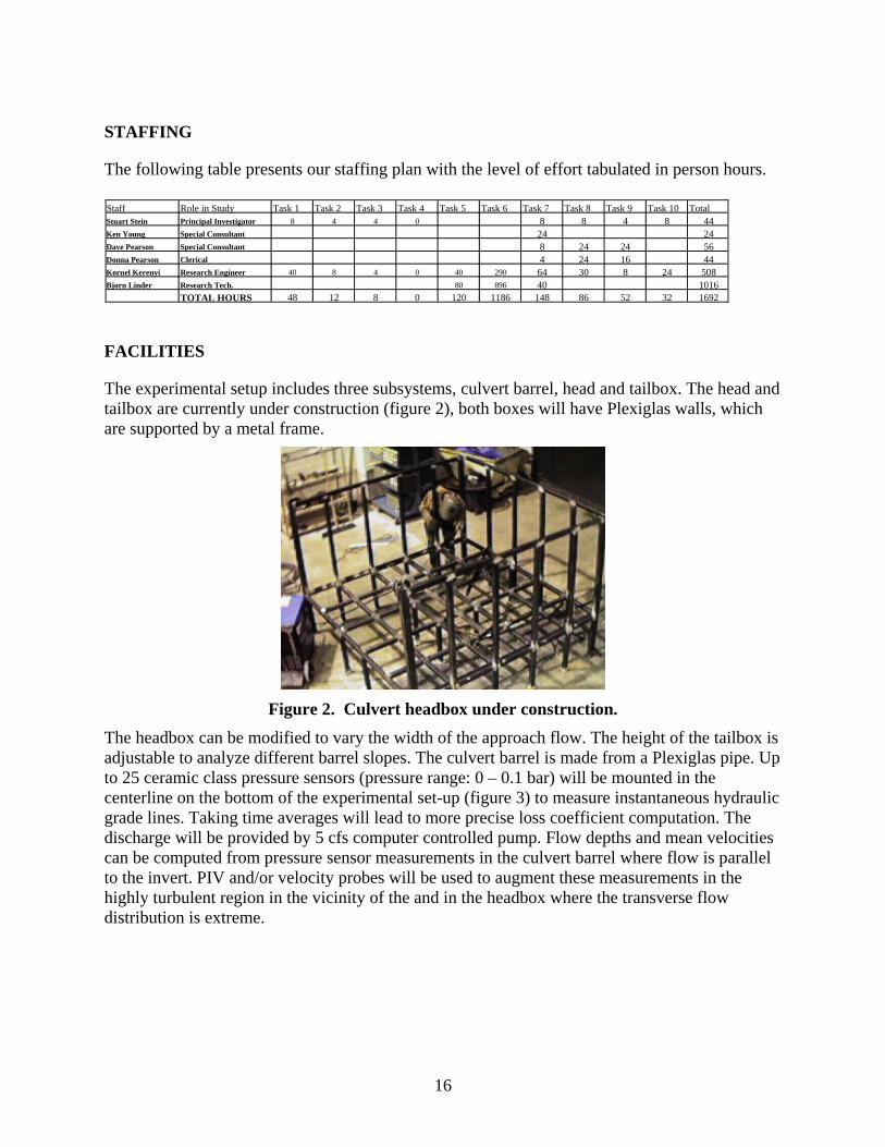
The experimental setup includes three subsystems, culvert barrel, head and tailbox. The head and tailbox are currently under construction (figure 2), both boxes will have Plexiglas walls, which are supported by a metal frame.

Figure 2. Culvert headbox under construction.

The headbox can be modified to vary the width of the approach flow. The height of the tailbox is adjustable to analyze different barrel slopes. The culvert barrel is made from a Plexiglas pipe. Up to 25 ceramic class pressure sensors (pressure range: 0 – 0.1 bar) will be mounted in the centerline on the bottom of the experimental set-up (figure 3) to measure instantaneous hydraulic grade lines. Taking time averages will lead to more precise loss coefficient computation. The discharge will be provided by 5 cfs computer controlled pump. Flow depths and mean velocities can be computed from pressure sensor measurements in the culvert barrel where flow is parallel to the invert. PIV and/or velocity probes will be used to augment these measurements in the highly turbulent region in the vicinity of the and in the headbox where the transverse flow distribution is extreme.

Staff Role in Study Task 1 Task 2 Task 3 Task 4 Task 5 Task 6 Task 7 Task 8 Task 9 Task 10 TotalStuart Stein Principal Investigator 8 4 4 0 8 8 4 8 44Ken Young Special Consultant 24 24Dave Pearson Special Consultant 8 24 24 56Donna Pearson Clerical 4 24 16 44Kornel Kerenyi Research Engineer 40 8 4 0 40 290 64 30 8 24 508Bjorn Linder Research Tech. 80 896 40 1016

TOTAL HOURS 48 12 8 0 120 1186 148 86 52 32 1692

17

Figure 3. Arrangement of the ceramic class pressure sensors.

To measure instantaneous velocity flow fields the particle image velocimetry technique (PIV) is used. PIV utilizes a focused light source, a high-resolution digital camera, and sophisticated computer logic to trace particle movements. This technology makes it possible to accurately measure velocity in complex situations such as flow into culverts. The experimental set-up of a PIV system typically consists of several subsystems (figure 4). In most applications tracer particles have to be added to the flow. These particles have to be illuminated in a plane of the flow at least twice within a short time interval. The light scattered by the particles has to be recorded either on a single frame or on a sequence of frames. The displacement of the particle images between the light pulses has to be determined through evaluation of the PIV recordings.

Figure 4. Experimental set up for Particle Image Velocimetry.

19

CHAPTER 3. LITERATURE REVIEW

The most comprehensive publication available in the literature is FHWA’s HDS-5 “Hydraulic Design of Highway Culverts” (see Normann, et al., 1985) which is a synthesis of culvert research including the classic studies done for the Bureau of Public Roads by the National Bureau of Standards during the 1950’s (see French, 1955, 1956, 1957, 1961 and 1966). It features sections on design considerations, conventional culvert design, tapered inlets, box culverts, circular pipe culverts, storage routing and special considerations. Appendices include design methods and equations, barrel resistance and design charts, tables and forms.

HDS-5 defines culvert hydraulics in terms of inlet and outlet control depending on the variables that influence the head required to push flow through the barrel. Inlet control occurs for steep culverts flowing free surface where flow goes through critical depth near the inlet. Flow in the culvert barrel below the critical depth section is supercritical flow that does not propagate downstream surface disturbances upstream. The only variables that affect the headwater are the discharge intensity and the geometry of the inlet. Outlet control occurs for mild slope culverts where free surface flow is subcritical and for any slope when the barrel is completely submerged. In this case the tailwater, which is typically known, is the control and the headwater is affected by tailwater depth, outlet loss, friction loss, elevation difference and the entrance loss, which is a function of discharge intensity and inlet geometry.

Outlet control is the more general case where the entrance loss is just one component that affects the headwater and usually is not the dominant component compared to the tailwater elevation and the friction in the barrel. The entrance loss is assumed to be a fraction of the velocity head in the barrel and is expressed as a coefficient times the velocity head. HDS-5 lists the entrance-loss coefficients as a single, constant value for each inlet shape. There is no distinction between high flows and low flows, but HDS-5 is a hydraulic design manual; so it is reasonable to expect coefficients to be more related to high flows. It is reasonable to expect some variation in this coefficient at low flows because the effective inlet shape changes when only a portion of it is in the flow zone.

Inlet control is the special case where the inlet geometry and corresponding entrance loss is the dominant component that affects the headwater. Regression equations have been developed, for each inlet shape, to express headwater as a function of discharge intensity directly or to compute a loss component that can be added to the critical head to yield headwater. These regression equations apply for a range of discharge intensities that include low flows. HDS-5 lists the regression coefficients for predetermined equation forms for each inlet shape.

During the late 1980’s there was a lot of interest in the hydraulics of long-span culverts, which were frequently proposed as low-cost alternatives to short bridges. Laboratory experiments at the FHWA Hydraulics Laboratory (see unpublished report by Jones, et al., 1991) were conducted to investigate effects of some of the characteristic features of long-span culverts namely culvert shape, span-to-rise ratio and contraction ratio. Experiments were conducted in the six-ft-wide by seventy-ft-long tilting flume set at a slope expected to generate inlet control. Culvert shapes included circular, which was used as a

20

benchmark, semicircular, high-profile arches and metal box geometries commonly used for long-span installations. Inlet geometry for all shapes was a thin projecting edge with no flared wing walls. Culvert shape seemed to have very little effect at the higher discharges for submerged flow, but the high-profile arch shape appeared to have lower relative entrance losses at the lower discharges for unsubmerged flow. There was no logical explanation for apparent advantage for the high-profile arch at low flows. The span-to-rise ratio was varied by testing three metal box culvert geometries referred to as a high box, a mid box and a low box with span-to-rise ratios of 2.0, 3.25 and 4.5, respectively. The span was held constant (at 20 in) while the rise varied in these experiments and the shapes varied slightly because the metal boxes were not actually rectangles, rather had rounded corners and resembled arches more than they did rectangles. The general trend was the higher the span-to-rise ratio, the lower the efficiency. In other words, for a thin edge projecting inlet, where there is no bevel to streamline the flow over the top edge, increasing span to rise actually increased the headwater required to convey a given discharge intensity through the inlet. The contraction ratio, approach channel width divided by the culvert width, varied from 6.0 to 1.5. It appears that the lower the contraction ratio the higher the efficiency, but the primary conclusion from this part of the study was that the headwater (HW) in HDS-5 is the specific energy head and not just the hydraulic grade line depth as is often presumed. To make the data agree with the performance curves shown in HDS-5 for the benchmark shape, it was necessary to include the approach-flow velocity head in the HW computations. Long span culverts are typically nearly the full width of the approach channel, the contraction ratios are small and the approach flow velocity is almost as high as the velocity in the culvert. This study was conducted to gain insight about the hydraulics of long span culverts but the results were never published.

A study conducted at the FHWA Hydraulics Laboratory for South Dakota DOT compared hydraulic performance of precast inlet configurations to traditional 30-degree flared-wing-wall inlets for box culverts (see Graziano, et al., 2001). Six culvert models constructed of plywood were tested for both inlet and outlet control water depths were measured through ports in the flooring via Tygon tubing connected to a pressure transducer. Box culverts with single 6 ft x 6 ft, 8 ft x 8 ft, 9 ft x 9 ft and 12 ft x 12 ft barrels 30-degree-wing walls were modeled in this study. Model scales of 1:10.67, 1:15 and 1:16 were selected to use stock thickness materials to simulate culvert wall thickness and wing-wall thickness. Two slopes, 3 percent and 1.75 percent, were used in the experiments. Effects of wing-wall miters (embankment slope), straight-cut bevels, culvert barrel slopes, wing-wall flare, and parapets were compared.

Inlet-control design coefficients were developed by regressing experimental data using the inlet-control design equations found in HDS-5. A benchmark culvert model fabricated and tested to compare with HDS-5 Chart 8/3 as a check on experimental procedures. Inlet-control coefficients were derived for unsubmerged and submerged conditions for each culvert model and the outlet control entrance-loss coefficient, Ke, was computed for each culvert model.

The design coefficients for the benchmark model HDS-5 chart 8/3 did not match the values tabulated in HDS-5 very well for inlet control; however, the outlet control coefficient, Ke, experimental value was a close match to the tabulated value at 0.68

21

versus of 0.7. For unsubmerged conditions the miter slope, span-to-rise ratio and the culvert barrel slope appeared to have insignificant effect on the design coefficients. For submerged conditions the 3:1 miter is slightly more efficient than a 2:1 miter. In contrast to the observation noted for the long-span culvert study, the higher span-to-rise ratios improved culvert performance (reduced headwater for a given discharge intensity), but these models did not have the thin edge projecting inlet geometry. Parapets used to retain fill over the top plate appeared to improve rather than hinder culvert performance.

Overall the precast inlets with beveled edges were slightly better than the typical field-cast inlets without beveled edges but were not as good as the 30-degree-flared wing-wall inlet, but there were no attempts to optimize the bevels in that study. A number of general trends were noted, but there were no recommendations about how to modify FHWA manuals or computer programs to implement results from that study.

A study by Graziano, et al., (2001) for the Iowa DOT, also conducted at the FHWA Hydraulics laboratory, investigated the hydraulic performance of special Iowa DOT slope-tapered pipe culverts which consisted of off-the-shelf components including precast end sections, one eighth bends and pipe reducers that are readily available from pipe suppliers. The goals of the study were to derive design coefficients for a special Iowa slope tapered inlet consisting of off-the-shelf pipe reducers and bends for circular culverts and to investigate the sensitivity of performance to reducer length and taper ratio. The performance of the precast-end section, which is a flared-transition section that conforms to a 3:1 embankment slope, was compared to the performance of the HDS-5 chart 1/1 culvert which is a circular concrete culvert with a headwall and square edges.

Model scale ratios of 1:6.783 and 1:4.174 were used for this study. The headbox and tailbox were plywood versions of the culvert test facility that is currently in the laboratory. Hydraulic depths were measured by a single-pressure transducer connected through a switching block to pressure ports located along the culvert invert, in the headbox and in the tailbox. An adjustable tailgate was used to submerge the culvert to develop outlet control for a steep culvert.

For inlet control, the precast-end section by itself without the other components for the slope tapered inlet performed almost the same as the HDS-5 chart 1/1 inlet. When the precast end section was combined with the reducers and bends to make the Iowa slope taper unit, hydraulic performance was improved substantially. Performance was not sensitive to the taper ratio or whether one, two or three reducers were used to transition the taper.

For outlet control, the tabulated Ke value for the HDS-5 chart 1/1 inlet is 0.50, compared to Ke = 0.35 for the precast end section and Ke = 0.20 for the Iowa slope tapered inlet.

For inlet control, the design coefficients for the precast-end section were K = 0.51 and m = 0.55 for the unsubmerged form 2 equation and c = 0.021 and Y = 0.823 for the submerged flow equation. The corresponding coefficients for the Iowa slope tapered inlet were K = 0.477, m = 0.533, c = 0.025 and Y = 0.659.

GKY & Associates, Inc. (1998) consolidated design coefficients including the fifth-order polynomials that were used to code computer programs such as HY-8. Derivations for the various equations cited in HDS-5, a comprehensive set of design coefficients and

22

nomographs or performance curves for all of the inlets covered by HDS-5 plus several that were studied later are included in this report.

McEnroe and Johnson (1995) tested shop fabricated metal and precast-concrete-open-flared-end sections that are commonly available from pipe suppliers. They also studied the effects of flow bars and debris blockage on the hydraulic performance of the pipes.

They noted that HDS-5 provides little information on the hydraulic characteristics of these common end sections other than that “from limited hydraulic tests they are hydraulically equivalent in operation to a headwall in both inlet and outlet control.” Their experiments with two pipe sizes resulted in outlet control Ke values ranging from 0.24 to 0.31. Both the metal and concrete end sections had the larger value for the smaller pipe size and the lower value for the larger pipe size. The precast-concrete-open-flare-end section tested by McEnroe and Johnson was the same as the end section tested by Graziano for the Iowa DOT and is illustrated in figure 5. below. Graziano recommended a Ke value of 0.35 which is comparable to the 0.31 value found by McEnroe and Johnson for that end section.

Figure 5. Sketch of precast flared end section tested by Graziano and by McEnroe.

McEnroe and Johnson did not follow the HDS-5 pattern for presenting the inlet-control results; rather they provided three dimensionless component equations for each inlet. The first component equation essentially represents the unsubmerged condition. The second one represents the transition zone and the third one represents the submerged condition. The component equations for the prefabricated metal end section were:

41.0060.15

60.0

5≤≤⎟

⎟

⎠

⎞

⎜⎜

⎝

⎛=

DgQfor

DgQ

DHW

62.041.0023.023.255

≤≤+⎟⎟

⎠

⎞

⎜⎜

⎝

⎛=

DgQfor

DgQ

DHW

23

20.162.090.261.1289.15

2

55≤≤

⎟⎟

⎠

⎞

⎜⎜

⎝

⎛+

⎟⎟

⎠

⎞

⎜⎜

⎝

⎛−=

DgQfor

DgQ

DgQ

DHW

The component equations for the precast concrete end section were:

42.0053.15

55.0

5≤≤⎟

⎟

⎠

⎞

⎜⎜

⎝

⎛=

DgQfor

DgQ

DHW

68.042.0055.013.255

≤≤+⎟⎟

⎠

⎞

⎜⎜

⎝

⎛=

DgQfor

DgQ

DHW

30.168.050.250.1367.15

2

55≤≤

⎟⎟

⎠

⎞

⎜⎜

⎝

⎛+

⎟⎟

⎠

⎞

⎜⎜

⎝

⎛−=

DgQfor

DgQ

DgQ

DHW

The first equation in each set can readily be converted to the HDS-5 format to compare with Graziano’s results. The first component for the precast-concrete-end section can be written as

04.30515.0 2/1

55.0

2/1 ≤≤⎟⎟⎠

⎞⎜⎜⎝

⎛=

DAQfor

DAQK

DHW

U

where: KU = 1.0 for English units ; KU = 1.38 for SI units

The above expression is the form 2 equation for unsubmerged-inlet-control flow, which means McEnroe and Johnson got K=0.51 and M = 0.55 which were the exact values obtained by Graziano in a completely independent study.

Umbrell, et al., (2001) did a site-specific model study of a culvert installation consisting of a larger concrete culvert in series with a smaller culvert. The inlet was a 30-degree-

flared-wing wall which was tested with both culvert diameters. The Ke values ranged from 0.12 to 0.24, but the higher values tended to be for the larger pipe size and the lower discharges. Researchers attributed the differences to experimental scatter and proposed an average value of 0.14.

A current NCHRP study at Utah State University is investigating the effects of culvert geometry on hydraulic performance for circular culverts with buried inverts, composite roughness and other measures used to promote fish passage through culverts. Entrance-loss coefficients at low flows are of interest because fish passage criteria are based on average seasonal flows, not the higher flows used for culvert design.

Tullis (2004) observed that the entrance-loss coefficients for outlet control were not constant values for an inlet geometry as normally presented in the literature. There was considerable variation in the Ke values especially for low flows. Researchers

24

hypothesized that Ke might be a function of Reynolds number as illustrated in the conceptual sketch shown in figure 6 below. The implication of that observation is a little distressing because it would tend to complicate an otherwise simple computation. The entrance-loss coefficient seem to be higher at the lower Reynolds numbers, which means the larger culverts would tend to have lower loss coefficients. This hypothesis might help explain why McEnroe and Umbrell, et al., found smaller Ke’s for the larger models used in the tests.

0 0.5 1 1.5 2 2.5

HW/D

Ke

Re=200,000

Re=300,000

Re=100,000

Re=75,000

Figure 6. Conceptual sketch of entrance-loss coefficient related to Reynolds number (Tullis, 2004).

25

CHAPTER 4. THEORY AND DESIGN CALCULATIONS FOR INLET AND OUTLET CONTROL

The theory outlined in HDS-5 (Normann, et al., 1985) as described below is the basis for analyzing data from this study.

INLET-CONTROL HYDRAULICS OF CULVERTS

Empirical regression coefficients developed by fitting experimental data to semi theoretical equations are listed in HDS-5 for each inlet shape to relate headwater to discharge intensity for a range of flows.

Analysis of inlet-control data depends upon whether or not the inlet is submerged. If the inlet is not submerged, headwater can be expressed as a simple energy balance between the critical section and the upstream section, which are almost adjacent to one another or it can be analyzed as flow over a weir. Weir flow can be expressed as Q = f(HW)m or HW = f(Q)M, where a typical value of M is 2/3 or 0.667. If the inlet is submerged, flow through the inlet is conceptually like flow through an orifice, albeit an irregular shaped orifice. Orifice flow can be expressed as Q = C*A*(2g*h)0.5 or h = c(Q/A)2 where h is a depth measured from the center of the orifice. Since headwater depths are usually measured from the invert of a culvert a more general expression for the orifice flow is HW = c(Q/A)2 + Y, where Y is an offset distance.

Figure 7 illustrates an unsubmerged inlet-control condition. Experimental data from this type of condition have been analyzed two ways. First, a simple energy balance can be made between sections 1 and 2 illustrated in figure 7. The critical specific energy Hc can be computed for any culvert shape, although it is tedious computation for some shapes. Data is regressed to determine regression coefficients K and M for computing the entrance loss, He. HDS-5 describes this analysis as the form 1 analysis for unsubmerged inlet-control flow. Most of the circular culvert inlets listed in HDS-5 are based on the form 1 analysis. The other way to analyze this type of data is to treat it as flow over a weir as illustrated in the form 2 equation. Then the regression coefficients essentially absorb the critical specific energy control. All of the rectangular box culverts in HDS-5 are based on the form 2 equation and in all cases the exponent M was 0.667. Circular culverts and elliptical culverts with tapered throats are also based on the form 2 equation but the exponent M varies a little for these inlets.

Figure 7. Typical inlet-control flow condition.

26

Unsubmerged Form 1 S.

ADQKK

DH

DHW M

.uci 7050 +⎥⎦

⎤⎢⎣⎡+=

(1)

Unsubmerged Form 2 M

.ui

ADQKK

DHW

⎥⎦⎤

⎢⎣⎡= 50

(2)

For inlet control under submerged conditions, regression constants c and Y were determined using equation (3) of the inlet-control design equations in HDS-5 for each of the culvert models tested:

Submerged S.Y

ADQKc

DHW

.ui 70

2

50 ++⎥⎦⎤

⎢⎣⎡=

(3)

Where:

HWi = Headwater depth above inlet-control section invert (ft);

D = Interior height of culvert barrel (ft);

Hc = Specific head at critical depth (dc + Vc2 / 2g) (ft);

Q = Discharge (ft3/s);

A = Full cross sectional area of culvert barrel (ft2);

S = Culvert barrel slope (ft/ft);

K, M, c, Y = Regression constants; and

Ku = 1.811 for SI, 1.0 for ES.

OUTLET CONTROL HYDRAULICS OF CULVERTS

Outlet control is the general case that covers everything except the special case of free surface flow passing through critical flow near the inlet. Outlet control flow occurs anytime the barrel flows full throughout, as illustrated in figure 8, regardless of the slope of the culvert.

27

Figure 8. Outlet control for full-flow condition.

If the culvert is installed on a mild slope (0.7%), outlet control will occur for both a submerged or unsubmerged inlet and a submerged or unsubmerged outlet. If the culvert is installed on a steep slope (3%), outlet control will occur if the tailwater is sufficiently high to submerge the critical depth at the upstream end of the culvert or to cause full barrel flow throughout. If a culvert is installed on a steep slope and only a portion of the barrel is submerged, a hydraulic jump will occur in the barrel but the headwater will still be inlet control. The controlling relationship for outlet control is an energy balance between sections 1 and 2 as illustrated in figure 8, but now the two sections are separated by all the losses and elevation changes that occur between the tailwater channel and the approach channel. The outlet control head-discharge relationship; where head relates to the total energy, is shown in equation (4).

L

duo H

gVTW

gVHW ++=+

22

22

(4)

Where:

HWo = Headwater depth above the inlet invert (ft);

TW = Tailwater depth above the outlet invert (ft);

Vu = Approach velocity (ft/s);

Vd = Downstream velocity (ft/s); and

HL = Total energy loss.

The total energy losses include: inlet, exit and friction losses as shown in equation (5)

LoLfLeL HHHH ++= (5)

28

The entrance and exit losses are commonly expressed as a fraction of the barrel velocity head as demonstrated in equation (6) and (7).

⎟⎟⎠

⎞⎜⎜⎝

⎛=

gVKH eLe 2

2

(6)

⎥⎥⎦

⎤

⎢⎢⎣

⎡⎟⎟⎠

⎞⎜⎜⎝

⎛−⎟⎟

⎠

⎞⎜⎜⎝

⎛=

gV

gVKH d

oLo 22

22

(7)

Where:

Ke = Entrance-loss coefficient;

Ko = Exit-loss coefficient usually assumed to be 1.0 for design;

⎟⎟⎠

⎞⎜⎜⎝

⎛g

V2

2

= Velocity head inside the culvert barrel; and

⎟⎟⎠

⎞⎜⎜⎝

⎛

gVd

2

2

= Velocity head in the downstream channel near the outlet; frequently neglected in design.

Since this study was focused on the effects of inlet geometry, the primary emphasis was on the entrance-loss coefficient for outlet control, but exit losses were measured to determine if multiple barrels or skewed inlets affected the exit loss coefficient. It would be reasonable to express the entrance loss in terms of a difference in velocity heads, especially for wide culverts with low contraction ratios, but data would need to be analyzed that way to apply the coefficient to a difference in velocity heads.

29

CHAPTER 5. DATA ACQUISITION AND DATA ANALYSIS PROCEDURES

The following describes the data acquisition system used for the culvert study and explains the data analysis procedures.

DATA ACQUISITION FOR CULVERT SET-UP

The pressure sensors installed to measure the HGL, the flow meters to gauge discharge and the tailgate control for the culvert set-up are linked to National Instruments FieldPoint a modular distributed I/O (Input/Output) system. National Instruments FieldPoint is designed for measurement, control, and data logging applications that require reliable, rugged systems involving diverse sensors and actuators located centrally or spread over large distances. FieldPoint also gives you the flexibility to choose an open, standard networking technology such as Ethernet, serial, or wireless that best suits your application. At the FHWA Hydraulics Laboratory wireless networking technology is used to integrate Fieldpoint into the Lab data acquisition system. NI LabVIEW graphical development software is utilized to provide all the tools necessary to create measurement and control applications for FieldPoint.

The pressure sensors installed are Baumer Sensopress Type PCRD D015.14C.B110. The maximum pressure that can be applied to the sensor is 100 mbar or a 39-in water column.

For inlet-control tests only the tailbox pressure sensor readings were analyzed. For outlet control test the pressure sensor readings in head, barrels and tailbox were evaluated. To verify the pressure sensor data in the barrels, four standpipes per barrel were installed. Pressure sensors were mounted on the bottom of the standpipes. In addition to the pressure sensors a scale attached to side of the standpipes was used for manual readings of the water column in the standpipes. A scale was also mounted in the head and tailbox to validate the electronic readings.

DATA MANAGEMENT

Data management and data analysis were performed using the LabVIEW graphical programming technique for building applications such as testing and measurement, data acquisition, instrument control, data logging, measurement analysis, and report generation. LabVIEW programs are called virtual instruments (VI’s) because their appearance and operation imitate physical instruments such as oscilloscopes and multimeters. Every VI uses functions that manipulate input from the user interface or other sources and displays that information or moves it to other files or other computers.

Figure 9 shows the calculation procedure for obtaining the performance curves and inlet coefficients for each test.

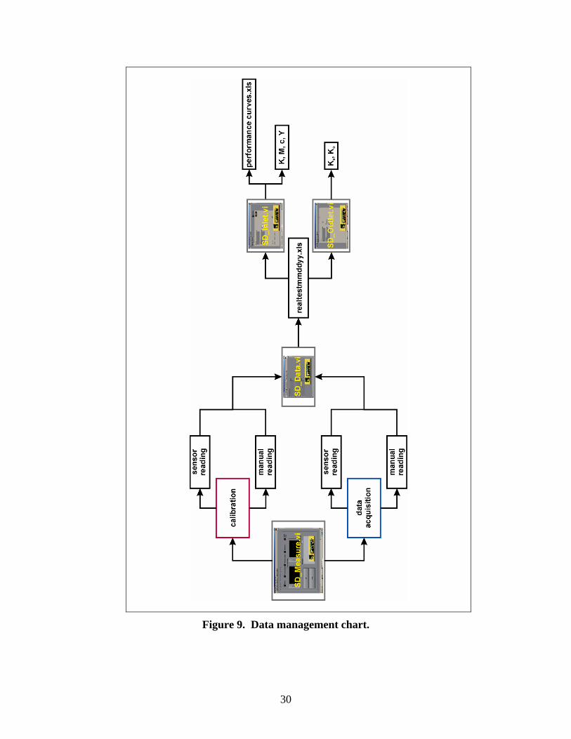
30

Figure 9. Data management chart.

31

DATA ANALYSIS FOR INLET CONTROL TESTS

Inlet-control coefficients, K and M, are derived directly from performance curve data (HWi /D vs Q/AD0.5) using

M

.ui

ADQKK

DHW

⎥⎦⎤

⎢⎣⎡= 50 (8)

from HDS-5 as a regression equation for unsubmerged flow conditions. For submerged flow, c and Y are derived from

S.YAD

QKcD

HW.

ui 702

50 ++⎥⎦⎤

⎢⎣⎡= (9)

Where:

HWi = Headwater depth above inlet-control section invert (ft);

D = Interior height of culvert barrel (ft);


A = Full cross sectional area of culvert barrel (ft2);

S = Culvert barrel slope (ft/ft);

K, M, c, Y = Regression constants; and

Ku = 1.811 for SI, 1.0 for ES.

When a full sequence of trial data is collected (ideally five unsubmerged and five submerged trials), the regression analysis is done using the nonlinear Levenberg-Marquardt fit algorithm in LabVIEW to determine the set of coefficients that minimize the chi-square quantity:

21

0

12 ∑−

=⎟⎟⎠

⎞⎜⎜⎝

⎛σ

−=χ

N

i i

Mii )a,...a;x(fy (10)

In this equation, xi and yi are the input data points, and f (xi; a1,…,aM) is the nonlinear function, where a1,…,aM are coefficients. If the measurement errors are independent and normally distributed with a constant standard deviation σi = σ, this is also the least-square estimation.

32

In addition to the proposed inlet coefficients (K, M, c, Y) fifth-order polynomials for inclusion in future updates to HDS-5 were derived to fit the unsubmerged and submerged data points (equation 11).

5

50

4

50

3

50

2

5050 ⎥⎦⎤

⎢⎣⎡+⎥⎦

⎤⎢⎣⎡+⎥⎦

⎤⎢⎣⎡+⎥⎦

⎤⎢⎣⎡+⎥⎦

⎤⎢⎣⎡+= .....

i

ADQf

ADQe

ADQd

ADQc

ADQba

DHW

(11

)

The best-fit coefficients were calculated using LabVIEW’s general polynomial fit virtual instrument, which is based on the Least Squares Procedure to estimate the best fit.

DATA ANALYSIS FOR OUTLET CONTROL TESTS

Outlet control entrance loss is just one component that is added to friction and outlet losses to relate headwater elevations to TW elevations. Data from outlet loss experiments require careful scrutiny to avoid reporting unreasonable results. The entrance-loss coefficient, Ke, for outlet control is computed from the relationship:

⎟⎟⎠

⎞⎜⎜⎝

⎛=

gVKH eLe 2

2

or ⎟⎟⎠

⎞⎜⎜⎝

⎛÷=

gVHK Lee 2

2

(12)

Where:

HLe is the entrance loss component that is usually computed for the design situation but is measured in the lab to compute Ke.

The technique used to measure HLe illustrated in figure 10 involves extrapolating EGL’s in the headbox and in the culvert barrel to a common plane and taking the difference in the EGL’s at that common plane. Common practice is to report an average design value of Ke that is a function of the inlet type only.

For higher discharge intensities, when the culvert barrel was at or near full, the computed Ke values were reasonably constant to warrant reporting an average value for design purposes. For the lower discharge intensities, when the culvert barrel was part-full throughout, the Ke values scatter considerably. This scatter is the result of the velocity head being very small and approaching zero for the very low discharges. In addition HLe is sensitive to the extrapolation process and to the flow distribution in the multiple barrels pushing the resolution limits of the pressure transducers (figure 11). The difficulties of the extrapolation process for low flows justify splitting Ke into an unsubmerged and submerged coefficient.

33

Figure 10. Technique to determine HLe.

Figure 11. Typical behavior of Ke vs. discharge intensity.

35

CHAPTER 6. EXPERIMENTAL PROCEDURES

MINI-FLUME EXPERIMENTS

The mini-flume was used to conduct experiments to optimize the bevel edge of the wing walls and top edge using two-dimensional particle image velocimetry (2D PIV) in a 2800-mm-long and 450-mm-wide flume (figure 12). The culvert model and bevel models (figure 13) were constructed with Plexiglas™ to avoid reflections (model scale 1:30). The upstream flow conditioning was achieved using filter mats and honeycomb flow straighteners. The sidewalls of the flume are made of glass, allowing excellent flow visibility. The flow discharge can be varied between 0 and 5 l/s. An ultrasonic distance meter can measure the flow depth. An electromagnetic velocity probe measures the approach velocity.

The 2-D PIV system typically consists of several subsystems. In most applications tracer particles are added to the flow. These particles are illuminated in a plane of the flow at least twice within a short time interval. The light scattered by the particles is recorded either on a single frame or on a sequence of frames. The displacement of the particle images between the light pulses is determined using cross correlation techniques. The camera used for PIV recordings is a Roper Scientific MEGAPLUS Model ES1.0 digital camera. The camera is a stand-alone device that is connected to frame grabber card (NI PXI 1422) using a PXI computer. To generate the light sheet, a double-pulsed Solo PIV 120 laser (figure 12) is used. The Solo PIV 120 laser is a compact, dual laser-head system designed to provide a highly stable green light source for PIV applications.

Figure 12. Mini-flume and PIV set-up.

36

Figure 13. Bevel models and PIV camera at culvert entrance.

PIV – post processing

The evaluation of the 2-D PIV data results in instantaneous velocity vectors of the flow field. To study the contracted area in the culvert, it was useful to integrate the velocity fields resulting in stream function and potential function. The integration is based on the assumption that the integrand, that is the flow field, is two-dimensional as well as incompressible. In this case, potential theory relates the velocity field, U = (U (X,Y), V (X,Y)), to the stream function Ψ which can be integrated over the domain (X,Y plane) as shown in figure 15. Fifty double-image frames were recorded to correlate 50 velocity flow field samples. The integration procedure for the stream functions was applied taking the average of the velocity flow field sequence.

Seven different bevel edge conditions were tested for the mini culvert set-up (figure 14). The criterion to determine the best bevel performance was the contracted distance outside the viscous boundary layer (effective flow depth at vena contracta).

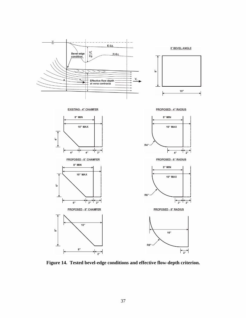
37

Figure 14. Tested bevel-edge conditions and effective flow-depth criterion.

38

∫∫ −=XY

dXVdYUΨ ∫∫ −=XY

dXVdYUΨ ∫∫ −=XY

dXVdYUΨ

Figure 15. Integration of the velocity flow field results in stream functions

to study flow contraction in the culvert.

CULVERT SET-UP EXPERIMENTS

The culvert set-up consists of two water tanks (a headbox 8-ft long by 8-ft wide by 4-ft high and a tailbox 8-ft long by 6-ft wide by 3-ft high) that were connected to the tested culvert barrel (figures 16 to 19). Five electronic pressure sensors were integrated into the bottom floor of the head and tailbox. An additional 40 pressure sensors measured the hydraulic grade line inside the culvert model barrels. The side rails of the tailbox supported a 2-D robot to measure the velocity distribution inside the tailbox (figure 20). The robot was automated to measure an area perpendicular to the main flow direction. A laser distance sensor recorded the position of the robot in the flow direction. An automated tailgate at the downstream end of the tailbox allowed for adjustment of the tail water depth. The culvert set-up was fully automated (pump/flowmeter and tailgate/pressure sensor control logic) and was network controlled (NI Fieldpoint system).

The experimental set-up is based on flow being in alignment with barrel. The barrels were tested for two different slope settings (3 percent and 0.7 percent). The purpose of the steep slope (3 percent) was to guarantee inlet-control conditions. The flat (0.7 percent) slope was designed to simulate outlet control conditions and was controlled by the adjustable tailgate. The pressure sensors in the culvert barrel were evaluated for subcritical flow for each outlet control test run. If this was not the case, the tailgate was lowered until outlet-control conditions were achieved. The velocity distribution at the exit of the culvert was also measured for each outlet-control test run

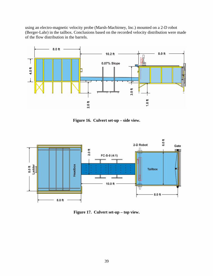
39

using an electro-magnetic velocity probe (Marsh-Macbirney, Inc.) mounted on a 2-D robot (Berger-Lahr) in the tailbox. Conclusions based on the recorded velocity distribution were made of the flow distribution in the barrels.

Figure 16. Culvert set-up – side view.

Figure 17. Culvert set-up – top view.

40

Figure 18. Culvert set-up – over view.

Figure 19. Culvert model barrels.

41

Figure 20. 2-D robot to measure velocity distribution in tailbox.

Inlet and culvert barrel models

All barrels used for the tests were fabricated out of Plexiglas™ consisting of two 61.25-in sections. Tapped holes for the pressure sensors were placed every 11.33 in on the bottom side of the culvert model barrels. Special holes on the top and bottom of the barrels provide a mounting for the corner fillets. Two sets of model fillets (0.5 in and 1 in) were fabricated using PVC material).

The inlet models were designed to consist of modular parts (wing walls, center walls, top plates) that were easily changed for various configurations. Tongue and groove connectors were used to assemble the models (figure 21).

Overview of models tested in the culvert set-up are listed in appendix A test matrix.

42

Figure 21. Groove connectors to assemble models.

43

CHAPTER 7. EXPERIMENTAL RESULTS

EFFECTS OF BEVELS AND CORNER FILLETS

Mini-flume test results for bevel effects

The small demonstration mini-flume was used with particle imaging velocimetry (PIV) to determine the best shape for the top edge from several alternate shapes that were suggested. The goal of the PIV mini-flume experiments was to accurately measure the flow field at the vena contracta. Post processing of PIV results provides streamlines that can be visually interpreted to show the shape that produces the maximum effective flow depth at the vena contracta. This shape is likely to have the least headloss when incorporated into the inlet geometry. The effective flow depth at the vena contracta for various bevel edge conditions are shown in figures 22 and 23.

For each experiment headwater and tailwater depths were measured. The difference of these depths versus the vena contracta measurement is plotted on figure 24. The results show that the 8-in-rounded-bevel edge produces the optimal geometric configuration.

Head loss experiments for bevel effects

The PIV mini-flume tests demonstrate which shape is best, but the question then is how much gain does this shape produce in the hydraulic performance. To answer that question, precast (PC) models, fabricated with the optimum bevel on the top plate and 4-in-radius-rounded bevels on the wing-wall edges, and field-cast (FC) models, fabricated with the SD standard straight bevel on the top plate and no bevels on the wing-wall edges, were tested in the culvert test facility. Additional tests were made with a model of the closest HDS-5 inlet which has zero-flare-angle-wing walls and no bevels on either the top plate or the wing walls and with a model of a field-cast-30-degree-flared-wing-wall culvert. Figures 25 and 26 show that the performance curve for the PC model with the optimum top plate bevel and rounded wing-wall edges is almost identical to the performance for the comparable field-cast model with zero-degree-wing-wall flare but with the straight-top-plate bevel and square-edge-wing-wall edges for unsubmerged flow when the top plate is not exposed to the flow. That comparison suggests that the four-in-radius bevels on the wing-wall edges do not contribute much gain. The gain shows up in the submerged condition with approximately 10 percent headwater reduction at the highest discharge intensities. Figure 27 shows that the optimum bevel model is almost as efficient as the 30-degree-flared-wing wall at the higher discharge intensities. The performance curves shown in figure 25 and 26 compare inlets and barrels with the same corner fillets to isolate the effects of the bevels. In South Dakota, the precast culverts are fabricated with 12-in-corner fillets and field-cast culverts are constructed with 6-in-corner fillets, but sizes of corner fillets were varied in these experiments to make clear comparisons.

44

Figure 22. Effective flow depth at vena contracta for non-rounded bevel edges.

45

Figure 23. Effective flow depth at vena contracta for rounded bevel edges.

46

45

46

47

48

49

50

51

52

53

54

55

56

57

58

59

60

22.5 23 23.5 24 24.5 25 25.5 26 26.5

difference head - tailwater [mm]

Effe

ctiv

e flo

w d

epth

at v

ena

cont

ract

a [m

m]

Series1

0 bevel angle

4" radius

8" radius

6" radius

6" chamfer

8" chamfer

4" chamfer

Figure 24. Effective flow depth vs. headwater/tailwater difference.

0

0.5

1

1.5

2

2.5

0 1 2 3 4 5 6 7

Q/AD0.5 (ft1/2/s)

HW

/D

FC-S-0PC-AHDS-5 8/3

Inlet ControlSubmerged

Inlet ControlUnsubmerged

single barrel0" fillets

FC-S-00o WW

45o chamfer-top plate

PC-A0o WW

8" radius-top bevel

HDS-5 8/30o WW

square-edge-top plate

Figure 25. Inlet-control performance curves FC-S-0 vs. PC-A with zero corner fillets.

47

0

0.5

1

1.5

2

2.5

0 1 2 3 4 5 6 7

Q/AD0.5 (ft1/2/s)

HW

/DFC-S-0PC-A



FC model0° WW

4"-straight-top-bevels6" fillets

PC model8"-radius-top-bevels

6" fillets

Figure 26. Inlet-control performance curves FX-S-0 vs. PC-A with 6-in corner fillets.

0

0.5

1

1.5

2

2.5

0 1 2 3 4 5 6 7

Q/AD0.5 (ft1/2/s)

HW

/D

FC-S-30FC-S-0PC-A



FC-S-0 model0o WW4"-straight-top-bevels6" fillets

PC-A model8"-radius top bevels6" fillets

FC-S-30 model30o WW4"-straight-top-bevels6" fillets

Figure 27. Inlet control: precast with 6-in fillets compared to field cast with 6-in fillets.

48

Effect of wing-wall-top-edge bevel

In response to comments on the draft report for this study, several extra tests were conducted to isolate the effects of the bevels on the edges of the wing walls. Earlier comparisons suggested that the wing-wall bevels had very little effect, but they were based on the unsubmerged flow only.

Since the models were precisely fabricated with clip-on components, it was relatively easy to mix and match components to isolate the wing-wall bevels. Two special models were tested. One was the FC model top plate with the PC model wing walls and is labeled FC-Hybrid in figure 28 below. The other was the PC top plate with the FC wing walls and is labeled PC-Hybrid in figure 28. In both cases the performance curves for the hybrid models plotted almost identically over the curves for the models with the other wing walls for both unsubmerged and submerged flow. The slight deviation in figure 29 is on the wrong side to suggest that there is any advantage to rounding the wing-wall edges.

0

0.5

1

1.5

2

2.5

0 1 2 3 4 5 6 7

Q/AD0.5 (ft1/2/s)

HW

/D

FC-S-0FC-hybird



single barrelFC top bevel

0" fillets

FC top platePC WW

PC top plate and WW

Figure 28. Inlet control: field-cast single inlet compared to a field-cast hybrid inlet with

4-in-radius bevel on side walls.

49

0

0.5

1

1.5

2

2.5

0 1 2 3 4 5 6 7

Q/AD0.5 (ft1/2/s)

HW

/DPC-APC-hybrid



single barrel8"-radius-top-bevel

0" fillets

PC top plateFC side wall

PC top plate and WW

Figure 29. Inlet control: precast single inlet compared to a precast hybrid inlet with no

bevel on side walls.

Effect of corner fillets

Corner fillets are fabrication expedients intended to minimize high stress areas in the corners for rectangular culvert shapes. The precast industry tends to use slightly larger corner fillets than might be used for field-cast construction. Obviously the corner fillets reduce flow area slightly, but the question is whether or not they affect hydraulic performance beyond that reduction in flow area. Varying the corner fillets was one of the most aggravating challenges in the experimental design for this study. Ideally the experimental coefficients would have been the same for the different fillets provide the correct net area was used in the computations. Then the same corner fillets could have been used for all of the tests and the culvert models would have been much simpler to fabricate.

Even though the net area was used in computations, the entrance-loss coefficients for outlet control did vary with the size of the corner fillets. The performance curves for inlet control show no difference using 0-in, 6-in or 12-in corner fillets. Figures 30 and 31 for field-cast and precast models, respectively, indicate that there is no headwater increase with fillet size for any given discharge intensity for inlet control. The entrance-loss coefficients for outlet control increase significantly for the 12-in fillets compared to the 6-in fillets and no fillets.

50

0

0.5

1

1.5

2

2.5

0 1 2 3 4 5 6 7

Q/AD0.5 (ft1/2/s)

HW

/DFC-S-0 0" filletsFC-S-0 6" filletsFC-S-0 12" fillets



0" fillets

6" fillets

12" fillets

FC-S-0 modelssingle barrel

0o flare

Figure 30. Inlet-control effects of corner fillets for the field-cast model.

0

0.5

1

1.5

2

2.5

0 1 2 3 4 5 6 7

Q/AD0.5 (ft1/2/s)

HW

/D

PC-A 0" filletsPC-A 6" filletsPC-A 12" fillets



PC-A model8"-radius-top-bevel

single barrel

0" fillets

6" fillets

12" fillets

Figure 31. Inlet-control effects of corner fillets for the precast model.

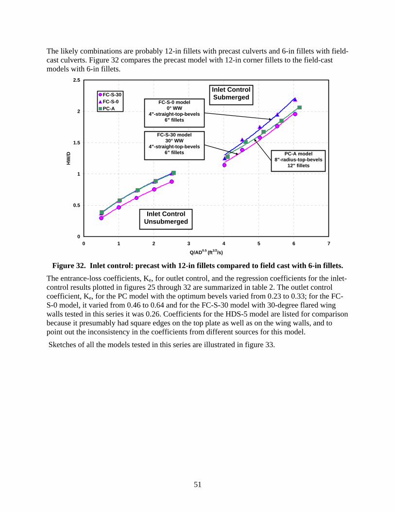
51

The likely combinations are probably 12-in fillets with precast culverts and 6-in fillets with field-cast culverts. Figure 32 compares the precast model with 12-in corner fillets to the field-cast models with 6-in fillets.

0

0.5

1

1.5

2

2.5

0 1 2 3 4 5 6 7

Q/AD0.5 (ft1/2/s)

HW

/D

FC-S-30FC-S-0PC-A



FC-S-0 model0° WW


FC-S-30 model30° WW

4"-straight-top-bevels6" fillets PC-A model

8"-radius-top-bevels12" fillets

Figure 32. Inlet control: precast with 12-in fillets compared to field cast with 6-in fillets.

The entrance-loss coefficients, Ke, for outlet control, and the regression coefficients for the inlet-control results plotted in figures 25 through 32 are summarized in table 2. The outlet control coefficient, Ke, for the PC model with the optimum bevels varied from 0.23 to 0.33; for the FC-S-0 model, it varied from 0.46 to 0.64 and for the FC-S-30 model with 30-degree flared wing walls tested in this series it was 0.26. Coefficients for the HDS-5 model are listed for comparison because it presumably had square edges on the top plate as well as on the wing walls, and to point out the inconsistency in the coefficients from different sources for this model.

Sketches of all the models tested in this series are illustrated in figure 33.

52

Table 2. Summary of inlet and outlet control coefficients for models tested for effects of bevel and corner fillets.

Model Span:Rise Slope Fillets Ke

K Form 1 Eq

M Form 1 Eq

K Form 2 Eq

M Form 2 Eq c Y

FC-S-0 1:1 0.7% 0” 0.46

0.7% 6” 0.50

0.7% 12” 0.62

3% 0” 0.45 0.55 0.64 0.0453 0.54

3% 6” 0.47 0.57 0.62 0.0448 0.56

3% 12” 0.64 0.58 0.61 0.0447 0.54

PC-A 1:1 0.7% 0” 0.27

0.7% 6” 0.25

0.7% 12” 0.33

3% 0” 0.25 0.56 0.63 0.0371 0.67

3% 6” 0.23 0.57 0.62 0.0371 0.67

3% 12” 0.30 0.57 0.61 0.0361 0.68

PC-A 2:1 3% 6” 0.35 0.60 0.56 0.0329 0.79

PC-A 2:1 3% 12” 0.40 0.60 0.55 0.0316 0.81

FC-S-30 1:1 0.7% 6” 0.26

HDS-5 Chart 8 Scale 3

NA NA 0” 0.70 0.061 0.75 0.0423 0.82

HDS-5 from Graziano (1996)

1:1 3% 0” 0.68 0.009 1.54 0.48 0.73 0.0435 0.62

1:1 3% 0” 0.0481 0.76 0.55 0.64 0.0469 0.55 HDS-5 from this study 0.7% 0” 0.79

53

HDS-5 Inlet 0o-flared-wing walls (WW), square-

edged at crown, no WW bevel

no corner fillets

FC-S-0 0o-flared-wing walls (WW), 4-

in-straight-top bevel, no WW bevel

no corner fillets

PC-A 0o wing walls (WW), 8-in-

radius-top bevel, 4-in-radius WW bevels

no corner fillets

FC-S-30 30o-flared-wing walls (WW), 4”-

straight-top bevel, no WW bevel

6-in-corner fillets

FC-S-0 0o-flared-wing walls (WW),

4-in-straight-top bevel, no WW bevel

6-in- and 12-in-corner fillets

PC-A 0o wing walls (WW), 8-in-

radius-top bevel, 4-in-radius WW bevels

6-in- and 12-in-corner fillets

Figure 33. Models tested for effects of bevels and corner fillets.

EFFECTS OF MULTIPLE BARRELS

Three questions need to be addressed with regard to multiple barrel culverts. First, is it reasonable and conservative or un-conservative to assume that single barrel coefficients are applicable for multiple barrel culverts? Second, does the advantage for flared wing walls diminish as the number of barrels or total span-to-rise ratio increases. In other words, is it less important to have flared wing walls as the number of barrels increases? Third, is there a hydraulic advantage to extending the center walls of a multiple barrel culvert onto the approach apron?

Sketches of all the models tested in this series are illustrated in figure 43.

Multiple barrels vs. single barrel

Figures 34 to 36 show that there is almost no difference in the performance of multiple barrels and a single barrel culvert for unsubmerged inlet control. Figures 34 and 35 show that there is a slight hydraulic advantage for the multiple barrel field-cast models compared to the single barrel model for submerged inlet control. Figure 36 indicates that there is a fairly substantial hydraulic advantage for the multiple-barrel precast models compared to the single barrel model for

54

submerged inlet control. Several of the precast models were retested to verify the multiple barrel results.

The outlet control results summarized in table 3 were a little inconsistent. The Ke values for the field-cast models with zero wing walls were almost identical for the single, double-, triple- and quad-barrel models and averaged 0.52. These results support the practice of using the single-barrel coefficients for multiple-barrel analyses. For the 30-degree-flared-wing-wall models the Ke values averaged 0.32 for the multiple-barrel models compared to Ke = 0.26 for the single-barrel model. That was not a big difference but was counter to the inlet-control indication in that the multiple barrels looked slightly worse than the single barrel for outlet control. For the precast models, the average Ke = 0.54 for the multiple barrel models compared to Ke = 0.33 for the single-barrel model.

Although there are slight differences in single- and multiple-barrel performance that are worthy of documentation, it is reasonable to combine the double-, triple-, and quad-barrel results.

0

0.5

1

1.5

2

2.5

0 1 2 3 4 5 6 7

Q/AD0.5 (ft1/2/s)

HW

/D

FC-S-0 singleFC-D-0 doubleFC-T-0 tripleFC-Q-0 quad



FC-X-0 models6" fillets0o flare

single

double

triple

quad

Figure 34. Inlet control: comparison FC-S-0 inlet, FC-D-0 inlet,

FC-T-0 inlet and FC-Q-0 inlet.

55

0

0.5

1

1.5

2

2.5

0 1 2 3 4 5 6 7

Q/AD0.5 (ft1/2/s)

HW

/D





single

double

triple

quad



0

0.5

1

1.5

2

2.5

0 1 2 3 4 5 6 7

Q/AD0.5 (ft1/2/s)

HW

/D

PC-A singlePC-B doublePC-C triplePC-D quad



PC-X models12" fillets

non-extended center wall

quad

triple

double

single

Figure 36. Inlet control: comparison PC-A inlet, PC-B inlet,

PC-C inlet and PC-D inlet.

56

Table 3. Summary of inlet- and outlet-control coefficients for models tested for effects of multiple barrels.

Model Slope Fillets Ke

K HDS-5 Form 2

Eq

M HDS-5 Form 2

Eq

c Y

FC-S-0 3% 6” 0.57 0.62 0.0448 0.56

0.7% 6” 0.50

FC-S-30 3% 6” 0.47 0.68 0.0394 0.53

0.7% 6” 0.26

FC-D-0 3% 6” 0.55 0.61 0.0391 0.66

0.7% 6” 0.52

FC-D-0-E 3% 6” 0.55 0.60 0.0394 0.65

0.7% 6” 0.53

FC-D-30 3% 6” 0.46 0.66 0.0366 0.61

0.7% 6” 0.34

FC-D-30-E 3% 6” 0.46 0.67 0.0381 0.59

0.7% 6” 0.31

FC-T-0 3% 6” 0.58 0.58 0.0377 0.69

0.7% 6” 0.54

FC-T-0-E 3% 6” 0.60 0.57 0.0405 0.67

0.7% 6” 0.58

FC-T-30 3% 6” 0.48 0.67 0.0379 0.60

0.7% 6” 0.31

FC-T-30-E 3% 6” 0.51 0.64 0.0405 0.60

0.7% 6” 0.32

FC-Q-0 3% 6” 0.55 0.61 0.0377 0.71

0.7% 6” 0.52

FC-Q-0-E 3% 6” 0.58 0.59 0.0418 0.64

0.7% 6” 0.50

57

Table 3. Summary of inlet- and outlet-control coefficients for models tested for effects of multiple barrels (cont’d).

Model Slope Fillets Ke

K HDS-5 Form 2

Eq

M HDS-5 Form 2

Eq c Y

FC-Q-30 3% 6” 0.47 0.71 0.0372 0.64

0.7% 6” 0.32

FC-Q-30-E 3% 6” 0.50 0.65 0.0398 0.60

0.7% 6” 0.34

PC-A 3% 12” 0.57 0.61 0.0361 0.68

0.7% 12” 0.33

PC-B 3% 12” 0.54 0.60 0.0253 0.90

0.7% 12” 0.49

PC-B-E 3% 12” 0.57 0.58 0.0315 0.81

0.7% 12” 0.56

PC-C 3% 12” 0.57 0.57 0.0219 0.98

0.7% 12” 0.54

PC-C-E 3% 12” 0.59 0.58 0.0263 0.91

0.7% 12” 0.51

PC-D 3% 12” 0.55 0.61 0.0250 0.92

0.7% 12” 0.59

PC-D-E 3% 12” 0.60 0.54 0.0296 0.85

0.7% 12” 0.58

Effect of wing-wall-flare angle

As the number of barrels increases, a smaller percentage of the flow is influenced by the wing walls and there is less advantage to having flared wing walls. The best way to visualize the effect is to observe the space (Δ) between the 30-degree and the 0-degree-flared-wing-wall performance curves in figures 37 to 40. Although the gap never closes, the curves do get closer as the number of barrels increases. It is interesting to observe that the PC multiple-barrel models with the optimum curved top plates actually outperformed the 30-degree-flared-wing-wall-multiple-barrel models at headwater to culvert depth ratios greater than 1.5 for the double, triple and quad barrel models. It is reasonable to expect that the optimum top-plate bevel will have a more pronounced effect on performance at the high headwater depths as the number of barrels and total span increases.

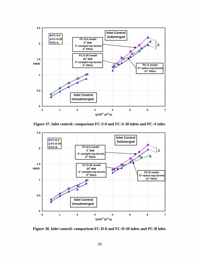
58

Figure 37. Inlet control: comparison FC-S-0 and FC-S-30 inlets and PC-A inlet.

Figure 38. Inlet control: comparison FC-D-0 and FC-D-30 inlets and PC-B inlet.

0

0.5

1

1.5

2

2.5

0 1 2 3 4 5 6 7

Q/AD0.5 (ft1/2/s)

HW/D

FC-S-0 FC-S-30 PC-A



FC-S-0 model0o WW


FC-S-30 model30o WW



Δ

0

0.5

1

1.5

2

2.5

0 1 2 3 4 5 6 7

Q/AD0.5 (ft1/2/s)

HW/D

FC-D-0 FC-D-30 PC-B



PC-B model 8"-radius-top-bevels

12" fillets

FC-D-0 model0o WW


FC-D-30 model30o WW


Δ

59

0

0.5

1

1.5

2

2.5

0 1 2 3 4 5 6 7

Q/AD0.5 (ft1/2/s)

HW

/DFC-T-0FC-T-30PC-C


Inlet ControlUn-Submerged

PC-C model8"-radius-top-bevels

12" fillets

FC-T-30 model30o WW


FC-T-0 model30o WW


Δ

Figure 39. Inlet control: comparison FC-T-0 and FC-T-30 inlets and PC-C inlet.

0

0.5

1

1.5

2

2.5

0 1 2 3 4 5 6 7

Q/AD0.5 (ft1/2/s)

HW

/D

FC-Q-0FC-Q-30PC-D



FC-Q-0 model0o WW


FC-Q-30 model30o WW


PC-D model8"-radius-top-bevels

12" fillets

Δ

Figure 40. Inlet control: comparison FC-Q-0 and FC-Q-30 inlets and PC-D inlet.

60

Effect of center-wall extension

There is no hydraulic advantage or disadvantage to extending center walls for multiple-barrel culverts. Figure 41 is typical of all of the results for the field-cast model results in that the performance for the extended center walls matched the performance for the non-extended center walls for the inlet-control tests. Field-cast inlets show nearly the same performance with and with out center wall extension. Figure 42 shows a similar comparison for the precast models with and without the extended center walls. The data point for the highest discharge intensity for the PC-B model was omitted from the trend line in figure 42 because it was considered to be an outlier point.

For outlet control, the Ke values tabulated in table 2 are almost identical in every case for the extended center walls and the corresponding nonextended center walls including the precast models.

Table 5 summarizes all the coefficients derived for the multiple-barrel series of tests. Figure 43 illustrates the models that were tested in this series.

0

0.5

1

1.5

2

2.5

0 1 2 3 4 5 6 7

Q/AD0.5 (ft1/2/s)

HW

/D

FC-D-30FC-D-30-E



FC-D-30 modeldouble barrel

6" fillets30° flare

Non-extended centerwall

Extended centerwall

Figure 41. Inlet control: comparison FC-D-30 and FC-D-30-E inlets.

61

0

0.5

1

1.5

2

2.5

0 1 2 3 4 5 6 7

Q/AD0.5 (ft1/2/s)

HW

/DPC-BPC-B-E



PC-Bdouble barrel

8"-radius-top-bevel12" fillets


Extended centerwall

Assumed outlier

Figure 42. Inlet control: comparison PC-B and PC-B-E inlets.

62

FC-S-30 30o flared WW, 4-in-straight-top bevel,

no WW bevel 6-in-corner fillets

FC-S-0 0o flared WW, 4-in-straight-top

bevel, no WW bevel

6-in-corner fillets

PC-A 0o WW, 8-in-radius-top

bevel, 4-in-radius-WW bevels

12-in-corner fillets

FC-D-30 30o flared WW, 4-in-straight-top

bevel, no WW bevel,

6-in-corner fillets

FC-D-0 0o flared WW, 4-in-straight-top

bevel, no WW bevel,

6-in-corner fillets

PC-B 0o WW, 8-in-radius-top bevel,

4-in-radius-WW bevels 12-in-corner fillets

FC-T-30

30o flared WW, 4-in-straight-top bevel,

no WW bevel, 6-in-corner fillets

FC-T-0 0o flared WW, 4-in-straight-top

bevel, no WW bevel, 6-in-corner fillets

PC-C 0o WW, 8-in-radius-top bevel, 4-in-radius-WW bevels, 12-in-corner fillets

Figure 43. Models tested for effects of multiple barrels.

63

FC-Q-30 30o flared WW, 4-in-straight-top

bevel, no WW bevel, 6-in-corner-fillets

FC-Q-0 0o flared WW, 4-in-straight-top

bevel, no WW bevel, 6-in-corner-fillets

PC-D 0o WW, 8-in-radius-top bevel,

4-in-radius-WW bevels, 12” corner fillets

FC-D-30-E 30o flared WW, 4-in-straight-top

bevel, no WW bevel,

extended center walls 6-in- corner fillets

FC-D-0-E 0o flared WW, 4-in-straight-top

bevel, no WW bevel,

extended center walls 6-in-corner fillets

PC-B-E 0o WW, 8-in-radius-top bevel,

4-in-radius-WW bevels extended center walls


FC-T-30-E


no WW bevel, extended center walls

6-in-corner fillets

FC-T-0-E 0o flared WW, 4-in-straight-top

bevel, no WW bevel,


PC-C-E 0o WW, 8-in-radius-top bevel,

4-in-radius-WW bevels, extended center walls,


FC-Q-30-E


no WW bevel, extended center walls

6-in-corner fillets

FC-Q-0-E 0o flared WW, 4-in-straight-top

bevel, no WW bevel,


PC-D-E 0o WW, 8-in-radius-top bevel,

4-in-radius-WW bevels, extended center walls


Figure 43. Models tested for effects of multiple barrels (cont’d).

64

EFFECTS OF SPAN-TO-RISE RATIO

Multiple span to rise vs. basic 1:1 span to rise

For inlet control, figure 44 shows that there may be a very slight loss in performance as the span-to-rise ratio increases for unsubmerged flow but almost no effect for submerged flow of the field-cast models with 0-degree wing walls (FC-S-0). Figure 45 shows similar results for the precast (PC) models. Figure 46 shows that there is a discernable decrease in performance in the submerged flow zone as the span-to-rise ratio increases for the field-cast models with 30-degree wing walls (FC-S-30) This decrease in performance is attributed in part to the diminishing effects of the wing-wall flare angle with increasing span to rise as discussed in the next section.

For outlet control, the entrance-loss coefficients, Ke varied from 0.32 for the 3:1 span-to-rise ratio to 0.46 for 1:1 ratio, but there was no clear trend and the variation can be attributed to experimental scatter for the FC-S-0 models. Similarly, the entrance-loss coefficients, Ke varied from 0.26 for the 4:1 span-to-rise ratio to 0.34 for the 2:1 ratio but there was no clear trend for the PC-A models. There was a slight trend in the entrance-loss coefficients for the FC-S-30 models in that Ke was 0.27 for the 1:1 and 2:1 span-to-rise ratios and was 0.19 and 0.18 for the 3:1 and 4:1 ratios, respectively, but the trend is just opposite from the effect observed for the inlet-control tests. A reasonable conclusion from the outlet control results is that the variations are experimental scatter and that the basic 1:1 model entrance-loss coefficients can be applied for various span-to-rise ratios.

Models tested in this series are illustrated in figure 51.

0

0.5

1

1.5

2

2.5

0 1 2 3 4 5 6 7

Q/AD0.5 (ft1/2/s)

HW

/D

FC-S-0 1:1 Span to riseFC-S-0 2:1 Span to riseFC-S-0 3:1 Span to riseFC-S-0 4:1 Span to rise



FC-S-0 models0" fillets0o flare

1:1 Span to rise

4:1 Span to rise

3:1 Span to rise

2:1 Span to rise

Figure 44. Inlet control: comparison of different span-to-rise FC-S-0 inlets.

65

0

0.5

1

1.5

2

2.5

0 1 2 3 4 5 6 7

Q/AD0.5 (ft1/2/s)

HW

/D

PC-A 1:1 Span to risePC-A 2:1 Span to risePC-A 3:1 Span to risePC-A 4:1 Span to rise



PC-A models0" fillets

8"-radius-top-bevels

4:1 Span to rise

3:1 Span to rise

2:1 Span to rise

1:1 Span to rise

Figure 45. Inlet control: comparison of different span-to-rise PC-A inlets.

0

0.5

1

1.5

2

2.5

0 1 2 3 4 5 6 7

Q/AD0.5 (ft1/2/s)

HW

/D





4:1 Span to rise

3:1 Span to rise

2:1 Span to rise

1:1 Span to rise

Figure 46. Inlet control: comparison of different span-to-rise FC-S-30 inlets.

66

Effect of wing-wall flare related to span-to-rise ratio

The inlet-control performance curves, figures 47 to 50 show that the wing-wall-flare angle has a diminishing effect as the span-to-rise ratio increases, which is analogous to the multiple barrel phenomenon. This observation can be visualized by inspecting the spacing, labeled as “Δ” in these figures, between the 0-degree wing-wall curves and the 30-degree wing-wall curves. As the span to rise and headwater depth ratios increase, the effect of the top plate bevel increases and the effect of the wing-wall flare angle decreases which explains why the PC models slightly outperformed the 30-degree wing-wall models for a few situations. This was similar to but less pronounced than the multiple-barrel comparison. Several of the tests plotted in figures 47 to 50 were repeated to confirm these results.

The outlet control entrance-loss coefficients listed in table 4 for the FC-S-30 models did not, however, support the assumption that wing-wall flare angle has diminishing effect as span to rise increases. The outlet control loss coefficient Ke was 0.27 for the basic 1:1 span-to-rise ratio, but decreased to 0.18 for the 4:1 ratio.

0

0.5

1

1.5

2

2.5

0 1 2 3 4 5 6 7

Q/AD0.5 (ft1/2/s)

HW

/D

FC-S-0FC-S-30PC-A


Inlet ControlUnsubmerged 1:1 Span to rise

FC model0° WW


FC model30° WW


PC model8"-radius-top-bevel

0" fillets

Δ

Figure 47. Inlet control: comparison FC-S-0, FC-S-30 inlets and

PC-A inlet (span to rise 1:1).

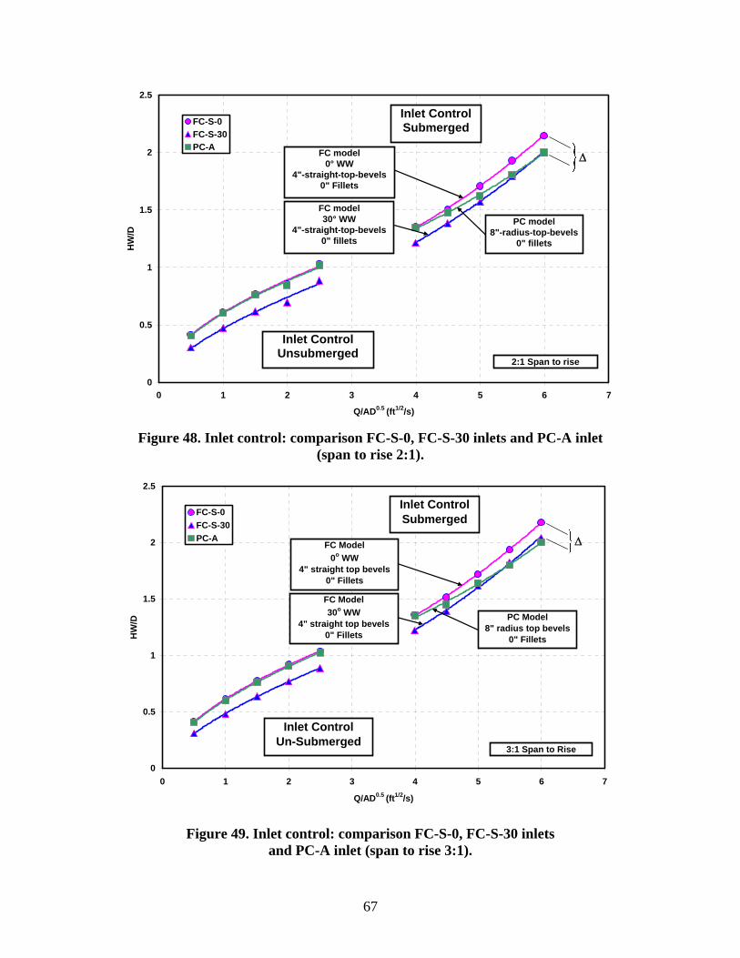
67

0

0.5

1

1.5

2

2.5

0 1 2 3 4 5 6 7

Q/AD0.5 (ft1/2/s)

HW

/DFC-S-0FC-S-30PC-A



FC model0° WW

4"-straight-top-bevels0" Fillets

FC model30° WW



0" fillets

2:1 Span to rise

Δ

Figure 48. Inlet control: comparison FC-S-0, FC-S-30 inlets and PC-A inlet

(span to rise 2:1).

0

0.5

1

1.5

2

2.5

0 1 2 3 4 5 6 7

Q/AD0.5 (ft1/2/s)

HW

/D

FC-S-0FC-S-30PC-A



FC Model0o WW

4" straight top bevels0" Fillets

FC Model30o WW

4" straight top bevels0" Fillets

PC Model8" radius top bevels

0" Fillets

3:1 Span to Rise

Δ

Figure 49. Inlet control: comparison FC-S-0, FC-S-30 inlets

and PC-A inlet (span to rise 3:1).

68

0

0.5

1

1.5

2

2.5

0 1 2 3 4 5 6 7

Q/AD0.5 (ft1/2/s)

HW

/DFC-S-0FC-S-30PC-A



FC model0° WW


FC model30° WW



0" fillets

4:1 Span to rise

Δ

Figure 50. Inlet control: comparison FC-S-0, FC-S-30 inlets

and PC-A inlet (span to rise 4:1).

Table 4. Summary of inlet and outlet control coefficients for models tested for effects of span-to-rise ratio.


K Form 1 Eq

M Form 1 Eq

K Form 2 Eq

M Form 2 Eq c Y

FC-S-0 1:1 3% 0” 0.55 0.64 0.0453 0.54 0.7% 0” 0.46

FC-S-0 2:1 3% 0” 0.60 0.56 0.0404 0.68 0.7% 0” 0.40

FC-S-0 3:1 3% 0” 0.61 0.58 0.0413 0.67 0.7% 0” 0.32

FC-S-0 4:1 3% 0” 0.62 0.57 0.0421 0.65 0.7% 0” 0.40

FC-S-30 1:1 3% 0” 0.44 0.74 0.0403 0.48 0.7% 0” 0.27

FC-S-30 2:1 3% 0” 0.47 0.66 0.0397 0.56 0.7% 0” 0.22

FC-S-30 3:1 3% 0” 0.48 0.66 0.0414 0.54 0.7% 0” 0.19

69

Table 4. Summary of inlet and outlet control coefficients for models tested for effects of span-to-rise ratio (con’t).


K Form 1 Eq

M Form 1 Eq

K Form 2 Eq

M Form 2 Eq c Y

FC-S-30 4:1 3% 0” 0.50 0.63 0.0410 0.59 0.7% 0” 0.18

PC-A 1:1 3% 0” 0.56 0.62 0.0371 0.66 0.7% 0” 0.27

PC-A 2:1 3% 0” 0.60 0.56 0.0329 0.79 0.7% 0” 0.34

PC-A 3:1 3% 0” 0.60 0.58 0.0331 0.79 0.7% 0” 0.29

PC-A 4:1 3% 0” 0.62 0.57 0.0340 0.79 0.7% 0” 0.26

70


no WW bevel, span to rise 1:1

0-in-corner fillets

FC-S-0 0o flared WW, 4-in-straight-

top bevel, no WW bevel, span to rise 1:1

0-in-corner fillets

PC-A 0o WW, 8-in-radius-top bevel,

4-in-radius WW bevels, span to rise 1:1

0-in-corner fillets



0-in-corner fillets


bevel, no WW bevel, span to rise 2:1

0-in-corner fillets



0-in-corner fillets

FC-S-30



0-in-corner fillets



0-in-corner fillets

PC-A 0o WW, 8-in-radius-top -bevel,


0-in-corner fillets

FC-S-30



0-in-corner fillets



0-in-corner fillets



0-in-corner fillets

Figure 51. Models tested for effects of span-to-rise ratio.

71

EFFECTS OF HEADWALL SKEW

Skewed headwalls as illustrated in figure 52 were tested for skew angles of 0o, 15o, 30o and 45o. The field-cast, triple-barrel, 30-degree wing wall (FC-T-30) and the field-cast single barrel, 30-degree wing wall with a 3:1 span-to-rise ratio (FC-S-30 (3:1)) models illustrated in figure 52 were used for these tests. Although it is not uncommon to see culvert installations with the approach flow actually skewed to the culvert alignment, this condition is considered bad practice and was not included in the test matrix.

Figure 52. Definition sketch for skew tests.

For inlet control, figure 53 shows that the performance curves for the three skewed headwalls (at 15 degrees, 30 degrees and 45 degrees) do cluster but are separated from the performance curve for the 0-degree headwall. Consequently, it is reasonable to combine the 15-degree, 30-degree and 45-degree skew curves for inlet control. The performance curve for the HDS-5 chart 12 scale 3 inlet, which is noted to be a good approximation for skews from 15 degrees to 45 degrees, is plotted in this figure for comparison, but it does not compare favorably with the skewed headwall models tested in this study. HDS-5 does not specify if that inlet represents a skewed headwall or a skewed flow alignment.

The outlet control entrance-loss coefficient could be averaged at Ke = 0.36 for 0-degree and 15-degree-skew angles, but increased to Ke = 0.46 for 30-degree and 45-degree skew angles. Table 5 summarizes the inlet and outlet control coefficients.

Models tested in this series are illustrated in figures 54 and 55. Figure 55 is the plan view of skewed inlets tested in this series.

72

0

0.5

1

1.5

2

2.5

0 1 2 3 4 5 6 7

Q/AD0.5 (ft1/2/s)

HW

/D

FC-T-30, 0° skewFC-T-30, 15° skewFC-T-30, 30° skewFC-T-30, 45° skewHDS-5 12/3, 15 to 45 degree skew



FC-T modelstriple barrel

0" fillets

15o skew

30o skew

45o skew

0o skew

HDS-5 12/3

Figure 53. Comparing HDS-5 12/3 inlet with a FC-T-30 inlet for 0-degree,

15-degree, 30-degree, and 45-degree skew angles.

FC-T-30

30o flared WW, 4-in-straight-top bevel, no

WW bevel, 0o skew

0-in-corner fillets

FC-T-30 30o flared WW, 4-in-straight-top bevel, no

WW bevel, 15o skew

0-in-corner fillets

FC-T-30 30o flared WW, 4-in-straight-top bevel, no

WW bevel, 30o skew

0-in-corner fillets

FC-T-30 30o flared WW, 4-in-

straight-top -bevel, no WW bevel,

45o skew 0-in-corner fillets


bevel, No WW bevel, 3:1 span to rise

0o skew 0-in-corner fillets

FC-S-30 30o flared WW, 4-in-straight-top -

bevel, no WW bevel,

3:1 span to rise, 30o skew

0-in-corner fillets

Figure 54. Models tested for effects of headwall skew: 15 degree, 30 degree, and 45 degree.

73

FC-T-30, 0-degree skew FC-T-30, 15-degree skew

FC-T-30, 30-degree skew FC-T-30, 45-degree skew

Figure 55. Plan view of skewed headwall models as tested.

Table 5. Summary of inlet and outlet control coefficients for models tested for effects of skewed headwall.

Model Span:Rise Skew Slope Fillets Ke

K HDS-5Form 2

Eq

M HDS-5 Form 2

Eq c Y FC-S-30 3:1 0° 3% 0” 0.48 0.66 0.0414 0.54 0.7% 0” 0.19 FC-S-30 3:1 30° 3% 0” 0.68 0.46 0.0306 0.89 0.7% 0” 0.39 FC-T-30 0° 3% 0” 0.48 0.67 0.0369 0.62 0.7% 0” 0.35 FC-T-30 15° 3% 0” 0.66 0.50 0.0289 0.95 0.7% 0” 0.36 FC-T-30 30° 3% 0” 0.70 0.48 0.0312 0.94 0.7% 0” 0.44 FC-T-30 45° 3% 0” 0.69 0.50 0.0224 1.10 0.7% 0” 0.46

74

OUTLET CONTROL ENTRANCE-LOSS COEFFICIENTS Ke FOR LOW FLOWS (UNSUBMERGED) CONDITIONS)

In culvert design, outlet control is typically associated with full or near full barrel flow. Outlet control can occur, however, for part full flow if the culvert barrel slope is flat enough. This condition is often encountered for environmental evaluations such as for fish passage. Outlet control loss coefficients are usually tabulated as constants for inlet types. Whereas some experimental scatter is expected, the scatter in the loss coefficients for unsubmerged flow in this study was so extreme that researchers decided to separate the unsubmerged data from the submerged data for the outlet control experiments. The unsubmerged loss coefficients are not considered reliable for implementation but the results and attempted analyses are useful for future research.

Table 6 summarizes the average entrance-loss coefficients for unsubmerged flow conditions. Not all the data points could be used to derive the average coefficients because some of the values were so far out of range that they were discounted during the data reduction phase of the study. The worst values seemed to occur at the lowest flows and the problem was attributed to the resolution limits of the pressure sensors. The accuracy of the current pressure transducer used is ± 5 mm (0.196 in). At the very low flows, the actual head losses being measured were less than the resolution of the pressure sensor. These measurements, which were mostly “noise” in the sensors, were divided by a velocity head, which was near zero, to compute the entrance-loss coefficients, which were often an order of magnitude larger than expected. In general the average entrance-loss coefficients for unsubmerged conditions tended to be higher than the coefficients for submerged conditions but it is difficult to determine if this tendency was real or just a result of the selection process of which values to include in the average.

Effects of Reynolds number on Ke

One hypothesis that was considered as a possible explanation for the large scatter in the entrance-loss coefficient at low flows was that Ke depended on Reynolds number. If that hypothesis were true, there should be a correlation between Ke and Reynolds number whether or not the culvert was submerged.

The Reynolds number hypothesis was tested using full barrel flow with the HDS-5 8/3 inlet because it was easier to control Reynolds numbers for full barrel flow than for free surface flow. Data was acquired with the Reynolds number held constant while the headwater depth ratio, Hw/D, varied. This process was repeated for a range of Reynolds numbers up to the maximum Reynolds number that could be accomplished with the experimental apparatus.

The Reynolds number is defined as a characteristic velocity times a characteristic length divided by the kinematic viscosity. The hydraulic radius times four was used as the characteristic diameter. Only submerged conditions were tested, so the characteristic length was the barrel diameter, D. The average flow velocity was calculated dividing the discharge by the area of the barrel. The entrance-loss coefficients for the HDS-5 8/3-inlet for Reynolds number range from 65000 to 260000 are presented in figure 56.

75

Table 6. Summary of outlet control entrance-loss coefficients, Ke, for low flows.

Model Slope Fillets No. BRLs Span:Rise Skew Unsubmerged

Ke * FC-S-0 0.7% 0” 1 1:1 0o 0.73 FC-S-0 0.7% 6” 1 1:1 0o 0.90 FC-S-0 0.7% 12” 1 1:1 0o 0.9 PC-A 0.7% 0” 1 1:1 0o 0.67 PC-A 0.7% 6” 1 1:1 0o 0.63 PC-A 0.7% 12” 1 1:1 0o 0.56 FC-S-30 0.7% 0” 1 1:1 0o 0.39 FC-S-30 0.7% 6” 1 1:1 0o 0.71 FC-S-0 0.7% 6” 1 1:1 0o 0.9 FC-S-30 0.7% 6” 1 1:1 0o 0.71 FC-D-0 0.7% 6” 2 1:1 0o 0.71 FC-D-0-E 0.7% 6” 2 1:1 0o 0.32 FC-D-30 0.7% 6” 2 1:1 0o 0.74 FC-D-30-E 0.7% 6” 2 1:1 0o 0.42 FC-T-0 0.7% 6” 3 1:1 0o 0.6 FC-T-0-E 0.7% 6” 3 1:1 0o 0.8 FC-T-30 0.7% 6” 3 1:1 0o 0.48 FC-T-30-E 0.7% 6” 3 1:1 0o 0.41 FC-Q-0 0.7% 6” 4 1:1 0o 0.83 FC-Q-0-E 3% 6” 4 1:1 0o 0.87 FC-Q-30 0.7% 6” 4 1:1 0o 0.38 FC-Q-30-E 0.7% 6” 4 1:1 0o 0.38 PC-A 0.7% 12” 1 1:1 0o 0.56 PC-B 0.7% 12” 2 1:1 0o 0.96 PC-B-E 0.7% 12” 2 1:1 0o 0.75 PC-C 0.7% 12” 3 1:1 0o 0.94 PC-C-E 0.7% 12” 3 1:1 0o 0.96 PC-D 0.7% 12” 4 1:1 0o 0.91 PC-D-E 0.7% 12” 4 1:1 0o 0.93 FC-S-0 0.7% 0” 1 1:1 0o 0.73 FC-S-0 0.7% 0” 1 2:1 0o 0.48 FC-S-0 0.7% 0” 1 3:1 0o 0.66 FC-S-0 0.7% 0” 1 4:1 0o 0.62 FC-S-30 0.7% 0” 1 1:1 0o 0.17 FC-S-30 0.7% 0” 1 2:1 0o 0.39 FC-S-30 0.7% 0” 1 3:1 0o 0.48 FC-S-30 0.7% 0” 1 4:1 0o 0.53 PC-A 0.7% 0” 1 1:1 0o 0.67 PC-A 0.7% 0” 1 2:1 0o 0.42

76

Table 6. Summary of outlet control entrance-loss coefficients, Ke, for low flows (cont’d).

Model Slope Fillets No. BRLs Span:Rise Skew Unsubmerged

Ke * PC-A 0.7% 0” 1 3:1 0o 0.80 PC-A 0.7% 0” 1 4:1 0o 0.69 FC-S-0 0.7% 0” 1 3:1 30° 0.84 FC-T-30 0.7% 0” 3 1:1 0° 0.47 FC-T-0 0.7% 0” 3 1:1 0° 0.86 FC-T-30 0.7% 0” 3 1:1 15° 0.43 FC-T-30 0.7% 0” 3 1:1 30° 0.85 FC-T-30 0.7% 0” 3 1:1 45° 0.9

* These values are not to be used due to resolution limits of pressure transducers used.

0

0.2

0.4

0.6

0.8

1

1.2

1.4

0 0.5 1 1.5 2 2.5 3 3.5 4Hw/D

Ke

6500081000130000146000162000178000194000227000260000

Figure 56. Entrance-loss coefficient for the HDS-5 8/3-inlet for different

Reynolds numbers.

The computed entrance-loss coefficients scattered between 0.6 and 0.95 for low Reynolds numbers and the scatter generally decreased with increasing Reynolds numbers, but there was no correlation between Ke and Reynolds number as illustrated in figure 56. Figure 57 shows that the standard deviation of the Ke data gradually decreases with increasing Reynolds number. This figure is included to demonstrate statistically that the scatter in Ke values decreases as Reynolds

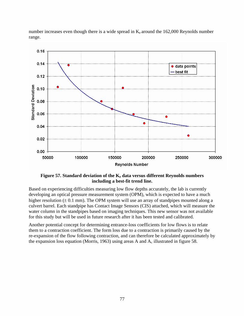
77

number increases even though there is a wide spread in Ke around the 162,000 Reynolds number range.

Figure 57. Standard deviation of the Ke data versus different Reynolds numbers

including a best-fit trend line.

Based on experiencing difficulties measuring low flow depths accurately, the lab is currently developing an optical pressure measurement system (OPM), which is expected to have a much higher resolution (± 0.1 mm). The OPM system will use an array of standpipes mounted along a culvert barrel. Each standpipe has Contact Image Sensors (CIS) attached, which will measure the water column in the standpipes based on imaging techniques. This new sensor was not available for this study but will be used in future research after it has been tested and calibrated.

Another potential concept for determining entrance-loss coefficients for low flows is to relate them to a contraction coefficient. The form loss due to a contraction is primarily caused by the re-expansion of the flow following contraction, and can therefore be calculated approximately by the expansion loss equation (Morris, 1963) using areas A and Ac illustrated in figure 58.

78

Figure 58. Culvert contraction.

By considering the flow expansion from the contracted section, of area Ac, to the normal section, of area A, the head loss is given by equation (13).

⎟⎟⎠

⎞⎜⎜⎝

⎛⎟⎟⎠

⎞⎜⎜⎝

⎛−=⎟⎟

⎠

⎞⎜⎜⎝

⎛⎟⎟⎠

⎞⎜⎜⎝

⎛−=⎟⎟

⎠

⎞⎜⎜⎝

⎛⎟⎟⎠

⎞⎜⎜⎝

⎛−==

gV

CgV

ACA

gV

AAHH

cccLcLe 2

112

12

1222222

(13)

The contraction coefficient Cc is equal to Ac / A, and depends on the area ratio A / Aa, the nature of the contraction or inlet geometry and slightly on the Reynolds number. To quantify the contracted area detailed velocity profiles can be measured in the contraction zone using either PIV (Particle Image Velocimetry) or LDA (Laser Doppler Anemometry). Based on the measured velocity vector fields streamlines can be integrated to compute the contracted area.

Neither of the latter two concepts has been tried yet because they were beyond the scope of this study, but they have promise and will be investigated for future studies.

OUTLET CONTROL EXIT-LOSS COEFFICIENTS, KO

The exit loss is a function of the change in velocity at the outlet of the culvert barrel. The exit loss, according to HDS-5 for a sudden expansion such as an end-wall, is

⎟⎟⎠

⎞⎜⎜⎝

⎛−=

gV

gV.H d

Lo 2201

22

(14)

Vd is the channel velocity downstream of the culvert. HDS-5 states that Ko = 1 may overestimate exit loss and a multiplier less then one can be used. If the downstream velocity is neglected, the exit loss is assumed to be the full-flow velocity head in the barrel.

79

Outlet loss data was analyzed by averaging the pressure tap measurements for the five pressure taps located downstream of the culvert outlet as illustrated in figures 59, 60 and 61 to determine the average HGL in the tailbox. The downstream velocity was computed from equation (14) where the area of flow was assumed to be the full width of the tailbox multiplied by the average tail water depth at the five pressure taps.

TWQVd

TBW= (15)

Where:


WTB = Full width of the tailbox (ft);

TW = Average tail water depth at five pressure taps (ft);

The velocity head Vd2/2g was added to the HGL elevation to establish an average downstream

EGL elevation, which was subtracted from the EGL at the end of the culvert to determine the head loss at the outlet, HLo. The exit loss coefficient, Ko, was then computed from equation (16):

⎥⎥⎦

⎤

⎢⎢⎣

⎡⎟⎟⎠

⎞⎜⎜⎝

⎛−⎟⎟

⎠

⎞⎜⎜⎝

⎛=

gV

gVKH d

oLo 22

22

(16)

The difficulty with this procedure is that the downstream velocity and therefore the computed coefficient is a function of the laboratory dimensions of the tailbox. The downstream velocity was artificially low because assumed flow area included a significant dead zone on each side of the culvert. That explains why some of the Ko values in table 7 are actually greater than 1.0.

In an effort to develop a more rational procedure for simulating downstream computation from a laboratory experimental setup, the velocity distributions in the tailbox were measured for several experiments. The goal was to analyze how velocity profiles expand moving further downstream and how the downstream velocity affects the exit loss. It would be reasonable to use the effective velocities in the expansion zone, illustrated in figures 59, 60 and 61, at each of the pressure taps to determine the EGL which could be projected to the plane of the culvert outlet to determine the exit head loss, HLo, as illustrated in figure 61. The effective velocities vary with distance downstream of the culvert and the challenge is deciding what velocity to use in equation (16) to compute Ko. An arbitrary, but reasonable, selection could be the velocity at three culvert widths downstream of the outlet.

Although this alternate procedure was not used for this study to compute the exit loss coefficients, the measurements in the expansion zone do provide good insight about flow downstream of culvert outlets.

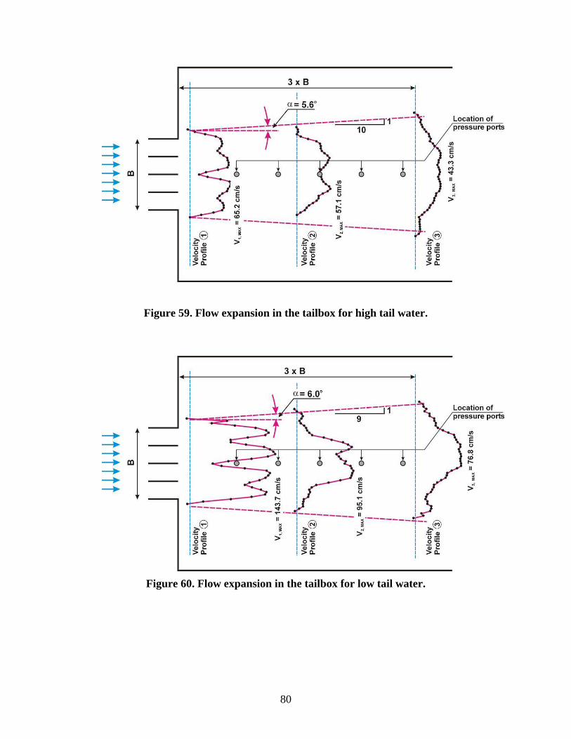
80

Figure 59. Flow expansion in the tailbox for high tail water.

Figure 60. Flow expansion in the tailbox for low tail water.

81

Note: Vertical to horizontal scale exaggerated by approximately 2:1

Figure 61. Vertical flow expansion in the tailbox and projected EGL.

The energy exit loss coefficients Ko are summarized in table 7 for different culvert barrel configurations tested. Each Ko value listed in table 7 is an average of several inlet geometries that had the same barrel configuration because, in the opinion of the researchers, the exit loss should not be significantly influenced by the inlet geometry.

82

Table 7. Summary of outlet loss coefficients.

Culvert barrel configuration Ko unsubmerged * Ko submerged

0.73 1.12

1.00 1.11

0.89 0.96

0.94 1.08

1.07 1.19

1.04 1.03

0.66 0.97

1.28 1.35

0.85 1.11

Skew 0.86 0.99

Skew 1.10 1.26

* These values are not to be used due to resolution limits of pressure transducers used.

83

FIFTH-ORDER POLYNOMIALS

In the area between submerged and unsubmerged flow conditions (HW/D), a transition area exists which neither the submerged or the unsubmerged forms of the equations provide accurate headwater predictions. An example of this transition area can be seen in figure 62. Fifth-order polynomials equations were developed that predict headwater in this region of uncertainty and over the entire range of measured HW/D ratios.

0

0.5

1

1.5

2

2.5

0 1 2 3 4 5 6 7

Q/AD0.5 (ft1/2/s)

HW

/D

5th order polynomial

Transition Area

Submerged regression data

Unsubmerged regression dataFC-S-0 modelsingle barrel

0" fillets

Figure 62. Transition between unsubmerged and submerged

inlet data control flow conditions. For culvert discharges within the range of the regression analysis, the polynomial equation gives a direct solution for inlet headwater, regardless of whether the inlet is submerged:

5

50

4

50

3

50

2

5050 ⎥⎦⎤

⎢⎣⎡+⎥⎦

⎤⎢⎣⎡+⎥⎦

⎤⎢⎣⎡+⎥⎦

⎤⎢⎣⎡+⎥⎦

⎤⎢⎣⎡+= .....

i

ADQf

ADQe

ADQd

ADQc

ADQba

DHW

(17)

Where:

a to f = Polynomial regression design coefficients.

The polynomial regression coefficients are presented in tables 8 to 11. Application of the polynomial equations presents numerical difficulties and errors at low and high values of HW/D. At low values, the HW/D prediction approaches the intercept coefficient, a, instead of zero as it should. At high values of HW/D, greater than about 2.3, the equations have a maximum. Therefore, the useful operating range of the polynomial equations is about 0.4 < HW/D < 2.3.

84

Table 8. Summary of polynomial regression coefficients for models tested for effects of bevels and corner fillets.

Fillet Span: Model (in.) Rise

a b c d e f

FC-S-0 0 1:1 0.211536 0.224341 0.208370 -0.121994 0.024676 -0.001609 FC-S-0 6 1:1 0.224471 0.247312 0.186514 -0.113509 0.023189 -0.001514 FC-S-0 12 1:1 0.245464 0.218175 0.210202 -0.121260 0.024063 -0.001536 PC-A 0 1:1 0.194217 0.310678 0.109365 -0.077409 0.016183 -0.001059 PC-A 6 1:1 0.203074 0.313529 0.107677 -0.076856 0.016046 -0.001046 PC-A 12 1:1 0.210576 0.314554 0.101951 -0.072650 0.014939 -0.000956 PC-A 6 2:1 0.186778 0.482282 -0.070441 -0.003094 0.003186 -0.000258 PC-A 12 2:1 0.189232 0.496842 -0.090840 0.005876 0.001525 -0.000152

Table 9. Summary of polynomial regression coefficients for models tested for effects of span-to-rise ratio.

Fillet Span: Model (in.) Rise

a b c d e f

FC-S-0 0 1:1 0.211536 0.224341 0.208370 -0.121994 0.024676 -0.001609 FC-S-0 0 2:1 0.207152 0.432143 -0.011800 -0.032349 0.009224 -0.000668 FC-S-0 0 3:1 0.227185 0.361402 0.077047 -0.069984 0.015731 -0.001063 FC-S-0 0 4:1 0.246621 0.315820 0.126140 -0.091438 0.019626 -0.001311 FC-S-30 0 1:1 0.163450 0.127103 0.256193 -0.131631 0.025211 -0.001601 FC-S-30 0 2:1 0.114704 0.376884 -0.007409 -0.024267 0.006977 -0.000502 FC-S-30 0 3:1 0.141479 0.321334 0.064086 -0.056126 0.012732 -0.000862 FC-S-30 0 4:1 0.246621 0.315820 0.126140 -0.091438 0.019626 -0.001311 PC-A 0 1:1 0.194217 0.310678 0.109365 -0.077409 0.016183 -0.001059 PC-A 0 2:1 0.154724 0.592825 -0.190065 0.048610 -0.006357 0.000370 PC-A 0 3:1 0.200747 0.424467 0.000339 -0.032906 0.008306 -0.000569 PC-A 0 4:1 0.220017 0.404031 0.029449 -0.046577 0.010869 -0.000734

85

Table 10. Summary of polynomial regression coefficients for models tested for effects of multiple barrels.

Fillet Num. of Model (in.) Barrels

a b c d e f

FC-S-0 6 1 0.224471 0.247312 0.186514 -0.113509 0.023189 -0.001514 FC-S-30 6 1 0.148953 0.250437 0.129334 -0.080435 0.016465 -0.001069 FC-D-0 6 2 0.154694 0.436581 -0.034324 -0.017500 0.006033 -0.000449 FC-D-0-E 6 2 0.168455 0.406534 -0.000921 -0.031807 0.008541 -0.000602 FC-D-30 6 2 0.101044 0.419241 -0.055078 -0.002691 0.002885 -0.000237 FC-D-30-E 6 2 0.103678 0.402060 -0.035969 -0.011102 0.004465 -0.000338 FC-T-0 6 3 0.185570 0.425924 -0.015139 -0.027376 0.007816 -0.000559 FC-T-0-E 6 3 0.220522 0.370427 0.057110 -0.060032 0.013803 -0.000936 FC-T-30 6 3 0.132482 0.340923 0.042681 -0.044257 0.010089 -0.000674 FC-T-30-E 6 3 0.146450 0.369886 0.018327 -0.037160 0.009256 -0.000639 FC-Q-0 6 4 0.154223 0.448350 -0.040698 -0.014061 0.005238 -0.000392 FC-Q-0-E 6 4 0.202572 0.369396 0.056302 -0.059162 0.013704 -0.000934 FC-Q-30 6 4 0.108394 0.355482 0.027300 -0.034330 0.007929 -0.000526 FC-Q-30-E 6 4 0.144926 0.350135 0.041407 -0.046111 0.010763 -0.000730 PC-A 12 1 0.210576 0.314554 0.101951 -0.072650 0.014939 -0.000956 PC-B 12 2 0.099284 0.607914 -0.221590 0.066777 -0.009847 0.000567 PC-B-E 12 2 0.149381 0.540449 -0.142259 0.029009 -0.002577 0.000099 PC-C 12 3 0.147326 0.545578 -0.146179 0.032208 -0.003485 0.000168 PC-C-E 12 3 0.153250 0.555777 -0.152070 0.035094 -0.004187 0.000219 PC-D 12 4 0.107009 0.600450 -0.207455 0.060926 -0.008924 0.000516 PC-D-E 12 4 0.158898 0.585920 -0.191810 0.048483 -0.005859 0.000294

Table 11. Summary of polynomial regression coefficients for models tested

for effects of skewed headwall.

Fillet Skew Model (in.) Angle

a b c d e f

FC-S-30 0 30 0.213123 0.685460 -0.298162 0.088583 -0.012236 0.000663 FC-T-30 0 0 0.128409 0.355047 0.026694 -0.037498 0.008897 -0.000603 FC-T-0 0 0 0.183389 0.409080 0.005613 -0.035825 0.009284 -0.000650 FC-T-30 0 15 0.182031 0.686256 -0.277043 0.082113 -0.011673 0.000654 FC-T-30 0 30 0.225978 0.658427 -0.240324 0.063449 -0.007969 0.000409 FC-T-30 0 45 0.187459 0.743672 -0.323642 0.103601 -0.016120 0.000958

87

CHAPTER 8. CONCLUSIONS AND RECOMMENDATIONS

During negotiations for this study the SD DOT technical review panel emphasized the need to have research results implemented in the HY-8 computer program “Hydraulic Design of Highway Culverts.” Since most highway designers use HY-8 or a similar program for hydraulic design of culverts, highway agencies don’t get much benefit from the research results until they are finally coded into a computer program. Even the Corps of Engineers HECRAS (Hydrologic Engineering Center River Analysis System) program, used for most water surface profile studies, includes the HY-8 logic for culvert evaluations. HY-8, as it is currently coded, does not allow for user defined design coefficients, which restricts practitioners from utilizing research results until they are finally coded into a program. Since HY-8 and other similar program are based on FHWA Hydraulic Design Series Number 5 (HDS-5) “Hydraulic Design of Highway Culverts,” the best approach for advancing the research to an implementation stage is to develop coefficients and performance curves in a format that is equivalent to the HDS-5 format, to derive 5th order polynomials to facilitate coding inlet-control performance curves in a computer program and to identify which results will have the most impact on the applicability or clarity of HDS-5.

HDS-5 is the most widely recognized publication available on culvert hydraulics. All of the inlets tested in this study were inlets covered in HDS-5 with various combinations of entrance improvements. HDS-5 does not include thumbnail sketches of the inlet configurations that go with the descriptions and it is sometimes difficult to visualize some of the details of the inlets. Nevertheless, we compared experimental results to published coefficients in HDS-5 where the inlets appeared to match the descriptions in HDS-5.

FINDINGS AND CONCLUSIONS

The following findings and conclusions are presented as a result of analyses of results from this study:

1. The discharge intensity is the primary independent variable used in culvert hydraulic analyses. As it is defined in HDS-5, it unnecessarily has units of ft1/2/s, but it could just as easily be defined as a dimensionless Froude number by including the acceleration of gravity in the denominator. Almost all other parameters in culvert hydraulics are dimensionless and to make that part also dimensionless would greatly facilitate converting from one system to another in this period of dual units; not to mention publishing a report in a SI- units-first environment for an audience that is primarily accustomed to customary English units.

2. The 8-in-rounded-radius-top-plate bevel was the optimum shape among six shapes tested. That radius is the full-wall thickness of the top plate. The optimum top-plate bevel does improve culvert performance significantly. The improvement is more pronounced for multiple barrels at higher headwater depths.

3. The 45o straight top-plate bevel, used for the SD DOT field-cast inlets, is an improvement over the square-edge-top plate specified in HDS-5 for concrete box culverts with 0o wing-wall flare angles.

88

4. The precast models with 0o wing-wall flare and optimum-curved-top-plate bevels, as tested in these experiments, performed consistently better than the comparable field-cast models with 0o wing-wall flare and the traditional 45o top-plate bevel. The precast models performed between the 0o and 30o flared-wing-wall-field-cast models, as illustrated in figures 71 and 72, except for multiple barrels at headwater depth ratios, HW/D, greater than 1.5 when the precast actually performed better than the 30o flared-wing-wall-field-cast model.

5. The rounded bevels for wing wall top edges had no discernible effect on culvert performance. The square-edge models performed as well as the models with rounded bevels.

6. The size of corner fillets had no discernible effect on the performance curves provided the net culvert area was used in the computation of the discharge intensity. The performance curves associated with various corner fillets in figures 30 and 31 can reasonably be combined as single curves as illustrated in figure 63. The inlet control tests showed no difference for the various corner fillet sizes. There was a slight difference in the outlet control coefficient for the 12-in fillets, but in the opinion of the authors that difference can be attributed to experimental scatter.

7. Multiple barrels had very little effect on performance curves for the field-cast (FC) models. The double, triple and quad curves figures 34 and 35 can reasonably be combined as single curves as illustrated in figures 64 and 65 and they could further be combined with the single-barrel curves without much loss in accuracy. This observation gives credibility to the common practice of using single-barrel design coefficients for multiple-barrel culverts.

8. Multiple barrels had more pronounced effect on performance curves for the precast-(PC) models with the optimum top bevels especially when the headwater depth ratio (HW/D) was greater than 1.5 as illustrated in figure 66. This was an unexpected result and several tests were rerun to confirm it. Most highway agencies, however, design culverts for headwater depth ratios below 1.5 and the practice of using single-barrel coefficients is still reasonable.

9. Span-to-rise ratios greater than 1:1 had very little effect on performance curves for either the field-cast or the precast-models as illustrated in figures 67 to 69, but the error in using the 1:1 design coefficients for wider span culverts tends to be on the unconservative side especially for inlets with flared wing-walls as illustrated in figure 68.

10. Extending the inner walls onto the approach apron for multiple-barrel culverts had no discernible effect on performance curves. There is no hydraulic advantage (or disadvantage) from extending the inner walls.

11. Skewed headwalls are unavoidable for some highway alignments, but they do have a detrimental effect on performance curves as illustrated in figure 70. Results from this study do not agree with limited guidance in HDS-5 for skewed headwalls.

12. Downstream exit flow from culvert models expanded at a gradual expansion angle of 5o

to 6o for a significant distance downstream of the culvert for both low and high tail-water depths.

89

13. Entrance loss coefficients for low-flows are important for fish passage considerations, but the unacceptable scatter, which can be attributed to instrumentation limitations for the very small losses that were associated with low flows makes those results unreliable and those coefficients for outlet control with free surface flow are not among the recommended results from this study. They are tabulated in an appendix for the benefit of other researchers who may have similar difficulties.

14. A commonly used prefabricated inlet for small circular culverts was highlighted from the literature review. Although it was not tested in this study, results were fairly consistent in two separate studies from the literature and design coefficients from those studies are considered reliable.

RECOMMENDATIONS

The following recommendations are for consideration by practitioners involved in field cast and pre-fabricated culvert installations:

1. Use the 8-in radius circular top plate bevel for prefabricated inlets where it is feasible to use more detailed forms.

2. Continue the practice of using straight chamfer on the top edge of wing walls because testing showed no benefit from rounding these edges.

3. Base decision to extend inner walls of multiple barrel culverts onto the apron on issues- such as debris control or aesthetics- other than hydraulics because testing showed no hydraulic advantage or disadvantage to extending these walls.

The following recommendations are for consideration as enhancements to future editions of hydraulic design manuals like HDS-5 and future generations of hydraulic design software like HY-8:

1. Redefine discharge intensity as a dimensionless parameter, 2/1)(gDAQ , to facilitate

conversion from one system of units to another. Keep the acceleration of gravity, g, in the independent parameter rather than imbedding it in the design coefficients.

2. Use thumbnail sketches, similar to those used in this report to clarify which inlet configurations correspond to design coefficients. Thumbnail sketches should also indicate test conditions embankment slope if they might affect range of applicability of design coefficients.

3. Define culvert area as net area rather than gross area where corner fillets are used. This should not affect current coefficients in HDS-5 because most historical testing was done without consideration to corner fillets.

4. Expand the table of design coefficients to include box culverts with 30° flare wing-walls and 45° straight beveled top plates as described as sketch 1 in table 12. This reflects the performance of SD’s field cast culverts with flared wing walls.

5. Expand the table of design coefficients to include 0° flare wing-walls box culverts with 45° straight beveled and rounded top plates as described for sketches 6 and 10 in table 12. This reflects performance of SD field cast and precast culverts with straight-mitered inlets.

90

6. Expand the table of design coefficients to include multiple barrel box culverts as described for sketches 2, 8 and 12 in table 12. This documents that multiple barrel culverts were tested and had very little effect on performance.

7. Expand the table of design coefficients to include wide-span box culverts as described for sketches 3, 9 and 13 in table 12. This documents that wide-span are slightly less effective than 1:1 span culverts for flared wing-wall installations.

8. Use the design coefficients in table 12 for inlets skewed to the flow direction due to skewed highway alignment relative to the flow direction. More research is needed to develop design coefficients for culvert barrels that are skewed to the flow direction. Even though this is considered “bad practice”, research is needed to show just how bad it is because it is a practice that is not all that uncommon.

9. Use table 13 for fifth-order polynomial coefficients that correspond to design coefficients in table 12. Fifth-order polynomials are coding expedients for computer software.

0

0.5

1

1.5

2

2.5

0 1 2 3 4 5 6 7

Q/AD0.5 (ft1/2/s)

HW

/D

FC-S-0PC-A



Single barrelcombined 0", 6" and 12" fillets

FC-S-0 model0o flare

PC-A model8"-radius-top-bevel

Figure 63. Combined corner fillet data for field-cast models with the 45-degree-straight-

top-plate bevel and precast models with the 8-in-radius-top-plate bevel (sketches 7, 14 and 10, 11 in figure 73).

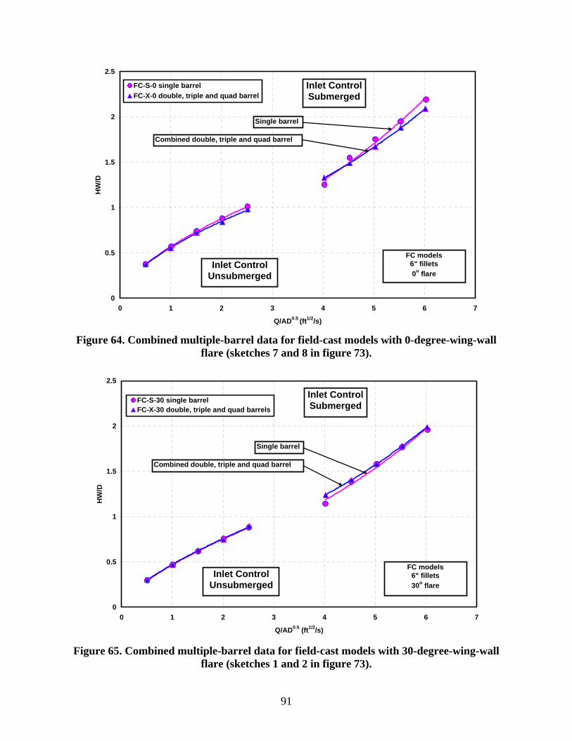
91

0

0.5

1

1.5

2

2.5

0 1 2 3 4 5 6 7

Q/AD0.5 (ft1/2/s)

HW

/DFC-S-0 single barrelFC-X-0 double, triple and quad barrel



FC models6" fillets0o flare

Single barrel

Combined double, triple and quad barrel

Figure 64. Combined multiple-barrel data for field-cast models with 0-degree-wing-wall

flare (sketches 7 and 8 in figure 73).

0

0.5

1

1.5

2

2.5

0 1 2 3 4 5 6 7

Q/AD0.5 (ft1/2/s)

HW

/D

FC-S-30 single barrelFC-X-30 double, triple and quad barrels




Single barrel


Figure 65. Combined multiple-barrel data for field-cast models with 30-degree-wing-wall

flare (sketches 1 and 2 in figure 73).

92

0

0.5

1

1.5

2

2.5

0 1 2 3 4 5 6 7

Q/AD0.5 (ft1/2/s)

HW

/DPC-A, single barrelPC-X, double, triple and quad barrel



PC models8"-radius-top-bevel

12" fillets

Single barrel


Figure 66. Combined multiple-barrel data for precast models with 0-degree-wing-wall flare

(sketches 11 and 12 in figure 73).

0

0.5

1

1.5

2

2.5

0 1 2 3 4 5 6 7

Q/AD0.5 (ft1/2/s)

HW

/D

1:1 Span to rise2:1, 3:1 and 4:1 Span to rise




Span to rise 1:1

Combined span to rise 2:1, 3:1 and 4:1

Figure 67. Combined span-to-rise data for field-cast models with 0-degree-wing-wall flare


93

0

0.5

1

1.5

2

2.5

0 1 2 3 4 5 6 7

Q/AD0.5 (ft1/2/s)

HW

/D

FC-S-30 1:1 Span to riseFC-S-30 2:1, 3:1 and 4:1 Span to rise




Span to rise 1:1

Combined Span to rise 2:1, 3:1 and 4:1

Figure 68. Combined span-to-rise data for field-cast models with 30-degree-wing-wall flare


0

0.5

1

1.5

2

2.5

0 1 2 3 4 5 6 7

Q/AD0.5 (ft1/2/s)

HW

/D

PC-A 1:1 Span to risePC-A 2:1, 3:1 and 4:1 Span to rise




8"-radius-top-bevel

Span to rise 1:1

Combined span to rise 2:1, 3:1 and 4:1

Figure 69. Combined span-to-rise data for precast models with 0-degree-wing-wall flare


94

0

0.5

1

1.5

2

2.5

0 1 2 3 4 5 6 7

Q/AD0.5 (ft1/2/s)

Hw

/D

FC-T-30, 15°, 30° and 45° skews averagedFC-T-30, 0° skew

FC - modeltriple barrel

0" fillets30° wing walls

averaged 15°, 30°, 45° skews

FC - modeltriple barrel

0" fillets30° wing walls

Figure 70. Skewed headwalls at 15-degree, 30-degree-, and 45-degree skews compared to 0-degree skew for triple-barrel-field-cast models with flared-wing walls (sketches 4 and 5 in

figure 73).

Figure 71. Precast single-barrel model compared to field-cast models (sketches 1, 7 and 11

in figure 73).

0

0.5

1

1.5

2

2.5

0 1 2 3 4 5 6 7

Q/AD0.5 (ft1/2/s)

HW/D

FC-S-0 FC-S-30 PC-A


Inlet Control Unsubmerged

FC-S-0 model0o WW


FC-S-30 model30o WW


8"-radius-top-bevels 12" fillets

95

0

0.5

1

1.5

2

2.5

0 1 2 3 4 5 6 7

Q/AD0.5 (ft1/2/s)

HW

/DFC-X-0FC-X-30PC-X


Inlet ControlUn-Submerged Multiple barrels

FC-X-0 model0o flarecombinded double, triple and quad barrel6" corner fillets

FC-X-30 model30o flarecombinded double, triple and quad barrel6" corner fillets

PC-X model8" radius top bevelcombinded double, triple and quad barrel12" corner fillets

Figure 72. Precast multiple-barrel models compared to field-cast models (sketches 7, 8, 1, 2

and 11, 12 in figure 73).

.

96

Table 12. Design coefficients suggested for future editions of HDS-5.

sketch HDS-5 chart

or table Description Ke K1 M1 K2 M2 c Y Box, reinforced concrete Chart 8/1 30o to 75o flared wing walls 0.026 1.00 0.38 0.81 Table 12 Square-edged crown 0.4 Table 12 Crown-edge rounded or top edge beveled 0.2 30o flared wing walls 1 This study Top-edge beveled at 45o 0.26 0.005 1.05 0.47 0.69 0.039 0.53 2 2,3 and 4 multiple barrels 0.32 0.55 0.60 0.037 0.68 3 2:1 to 4:1 span to rise 0.20 0.48 0.65 0.041 0.57 4 15o skewed headwall w/ multiple barrel 0.36 0.69 0.49 0.029 0.95 5 30o to 45o skewed headwall w/ multiple

barrels 0.45 0.69 0.49 0.027 1.02

0o flared wing walls (extension of sides) Chart 8/3 Square-edged at crown 0.7 0.061 0.75 0.047 0.82 6 This study Square-edged at crown 0.79 0.055 0.68 0.55 0.64 0.047 0.55 7 45o straight-bevel at crown w/ 0” and 6” corner

fillets 0.48 0.56 0.62 0.045 0.55

8 2, 3 and 4 multiple barrels 0.52 0.55 0.59 0.038 0.69 9 2:1 to 4:1 span to rise 0.37 0.61 0.57 0.041 0.67 10 Crown rounded at 8” radius, w/ 0” and 6” corner

fillets 0.24 0.56 0.62 0.038 0.67

11 Same as above w/ 12” corner fillets 0.3 0.56 0.62 0.036 0.68 12 2, 3 and 4 multiple barrels 0.54 0.55 0.60 0.023 0.94 13 2:1 to 4:1 span to rise 0.30 0.61 0.57 0.033 0.79

97

Table 13. Fifth-order-polynomial coefficients.

sketch

HDS-5 chart or

table Description a b c d e f Box, reinforced concrete Chart 8/1 30o to 75o flared wing walls 0.05067 0.65129 -0.24337 0.07045 -0.00897 0.000431 Table 12 Square-edged crown Table 12 Crown edge rounded or top edge beveled 30o flared wing walls 1 This study Top edge beveled at 45o 0.16345 0.127103 0.256193 -0.13163 0.025211 -0.0016 2 2,3 and 4 multiple barrels 0.112542 0.375074 0.002657 -0.02638 0.006867 -0.00047 3 2:1 to 4:1 span to rise -0.00048 0.006761 -0.02334 -0.02414 0.446748 0.199715 4 15o skewed headwall w/ multiple barrel 0.182031 0.686256 -0.27704 0.082113 -0.01167 0.000654 5 30o to 45o skewed headwall w/ multiple

barrels 0.206616 0.70114 -0.2818 0.083374 -0.01201 0.000681 0o flared wing walls (extension of sides) Chart 8/3 Square-edged at crown 6 This study Square-edged at crown 0.197052 0.265949 0.165865 -0.1043 0.021735 -0.00144 7 45o straight bevel at crown w/ 0” and 6” corner

fillets 0.226472 0.231777 0.200111 -0.11836 0.023887 -0.00155 8 2, 3 and 4 multiple barrels 0.164261 0.43842 -0.03128 -0.01919 0.006288 -0.00046 9 2:1 to 4:1 span to rise 0.227612 0.368733 0.064283 -0.06465 0.014855 -0.00101 10 Crown rounded at 8” radius

w/ 0” and 6” corner fillets 0.203424 0.31092 0.10783 -0.07609 0.015779 -0.00102 11 Same as above w/ 12” corner fillets 0.203424 0.31092 0.10783 -0.07609 0.015779 -0.00102 12 2, 3 and 4 multiple barrels 0.10315 0.619895 -0.23147 0.071093 -0.01075 0.000628 13 2:1 to 4:1 span to rise 0.199715 0.446748 -0.02414 -0.02334 0.006761 -0.00048

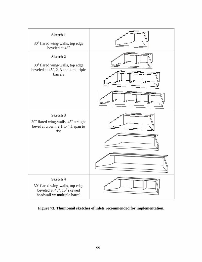
99

Sketch 1

30o flared wing-walls, top edge beveled at 45o

Sketch 2

30o flared wing-walls, top edge beveled at 45o, 2, 3 and 4 multiple

barrels

Sketch 3 30o flared wing-walls, 45o straight bevel at crown, 2:1 to 4:1 span to

rise


beveled at 45o, 15o skewed headwall w/ multiple barrel

Figure 73. Thumbnail sketches of inlets recommended for implementation.

100


beveled at 45o, 30o to 45o skewed headwall w/ multiple barrels

Sketch 6 0o flared wing-walls (extension of

sides), square-edged at crown

Sketch 7

0o flared wing-walls (extension of sides), 45o straight bevel at crown


Sketch 8

0o flared wing-walls (extension of sides), 45o straight bevel at crown,

2, 3 and 4 multiple barrels

Sketch 9 0o flared wing-walls (extension of sides), 45o straight bevel at crown,

2:1 to 4:1 span to rise


101

Sketch 10 0o flared wing-walls (extension of sides), crown rounded at 8”

radius, w/ 0” and 6” corner fillets

Sketch 11

0o flared wing-walls (extension of sides), crown rounded at 8”

radius, w/ 12” corner fillets

Sketch 12

0o flared wing-walls (extension of sides), crown rounded at 8”

radius, w/ 12” corner fillets, 2, 3 and 4 multiple barrels

Sketch 13 0o flared wing-walls (extension of sides), crown rounded at 8” radius, 2:1 to 4:1 span to rise


102

Sketch 14 0o flared wing-walls (extension of sides), 45o straight bevel at crown

w/ 12” corner fillets

Figure 73. Thumbnail sketches of inlets recommended for implementation (cont’d). Extended center walls does not effect flow conditions.

103

APPENDIX A. EXPANDED TEST MATRIX

This appendix is an expanded version of the negotiated test matrix described in chapter 2. The expanded matrix includes sketches, more detailed information about test conditions and extra tests that were conducted in response to questions posed during the study. It was posted in the lab and used as a checklist during the experimental phase.

Figure 74 illustrates the seven different bevel edge configurations that were tested in the mini flume to determine the best edge configuration. The criterion to determine the best edge configuration was the contracted distance outside the viscous boundary layer (effective flow depth at the vena contracta illustrated in figure 75). Particle image velocimetry (PIV) data were used to analyze the flow at the culvert entrance and to quantify the effective flow depth.

Tables 14 through 17 summarize tests performed in the culvert test facility for task six of the work plan to analyze the effects of bevels, multiple barrels, span-to-rise ratios, and skewed headwalls. Two extra inlets geometries, a FC-S-0 Hybrid and a PC-A Hybrid were tested in response to questions on the draft final report regarding the wing-wall bevels and are included in table 14. The FC-S-0 Hybrid was a combination of the field-cast-top-bevel with the precast wing-wall bevels and the PC-A Hybrid was a combination of the precast top bevel with the field-cast-square-edge-wing-walls.

104

Figure 74. Edge configurations tested in the mini-flume.

Figure 75. Streamlines from particle imaging velocimetry experiments used to quantify

effective flow depths at vena contracta.

105

Table 14. Task 6.1 tests performed in the culvert test facility to analyze the effects of bevels for wing walls and top edge.

Inlet No.

Model ID Sketch

Wing-Wall-Flare Angle Bevel

Corner Fillets

Culvert Box

Type Culvert Slopes

Tail Water

1.1 FC-S-0

0° 4”-straight-

top-bevel, no WW bevel

0” 6’x 6’ 0.03, 0.007

High, Low

1.2 FC-S-0

0° 4”-straight-


6” 6’x 6’ 0.03, 0.007

High, Low

1.3 FC-S-0

0° 4”-straight-


12” 6’x 6’ 0.03, 0.007

High, Low

1.4 PC-A

0°

8”-radius-top-bevel, 4”-radius

WW bevels

0” 6’x 6’ 0.03, 0.007

High, Low

1.5 PC-A

0°

8”-radius-top bevel, 4”-

radius WW bevels

6” 6’x 6’ 0.03, 0.007

High, Low

1.6 PC-A

0°


WW bevels

12” 6’x 6’ 0.03, 0.007

High, Low

1.7 PC-A

0°


WW bevels

6” 6’x 12’ 0.03 High, Low

1.8 PC-A

0°


WW bevels

12” 6’x 12’ 0.03 High, Low

1.9 FC-S-0 Hybrid

0°

4”-straight-top-bevel, 4”-radius

WW bevels

0” 6’x 6’ 0.03, High, Low

106

Table 14. Task 6.1 tests performed in the culvert test facility to analyze the effects of bevels for wing walls and top edge (cont’d).

Inlet No.

Model ID Sketch

Wing-wall Flare Angle Bevel

Corner Fillets

Culvert Box Type

Culvert Slopes

Tail Water

1.10 PC-A Hybrid

0° 8”-radius-top-bevel, no WW

bevels 0” 6’x 6’ 0.03, High, Low

Target discharge intensities for unsubmerged flow, Q/AD0.5 = 0.5, 1.0, 2.0, 3.5 and 4.0 (ft0.5/s) Target discharge intensities for submerged flow, Q/AD0.5 = 4.5, 5.0, 5.5, and 6.0 (ft0.5/s) Contraction ratio of headbox width to total span of culvert model was held constant at 2.67

107

Table 15. Task 6.2 tests performed to analyze the effects of multiple barrels.

Inlet No.

Model ID Sketch

Wing-Wall-Flare-Angle

Edge Conditions

Culvert Box Type

Culvert Slopes

Corner Fillets

No. of

Barrels Inner Wall

2.1 FC-S-0

0° 4”-straight-


6’x 6’ 0.03, 0.007 6” 1

2.2 FC-S-30

30° 4”-straight-


6’x 6’ 0.03, 0.007 6” 1

2.3 FC-D-0

0° 4”-straight-


2 - 6’x 6’ 0.03, 0.007 6” 2 Non extended

2.4 FC-D-0-E

0° 4”-straight-


2 - 6’x 6’ 0.03, 0.007 6” 2 Extended

2.5 FC-D-30

30°

4”-straight-top-bevel, no WW bevel

2 - 6’x 6’ 0.03, 0.007 6” 2 Non extended

2.6 FC-D-30-E

30° 4”-straight-


2 - 6’x 6’ 0.03, 0.007 6” 2 Extended

2.7 FC-T-0

0° 4”-straight-


3 - 6’x 6’ 0.03, 0.007 6” 3 Non extended

2.8 FC-T-0-E

0° 4”-straight-


3 - 6’x 6’ 0.03, 0.007 6” 3 Extended

2.9 FC-T-30

30° 4”-straight-


3 - 6’x 6’ 0.03, 0.007 6” 3 Non extended

2.10 FC-T-30-E

30° 4”-straight-


3 - 6’x 6’ 0.03, 0.007 6” 3 Extended

2.11 FC-Q-0

0° 4”-straight-


4 - 6’x 6’ 0.03, 0.007 6” 4 Non extended

108

Table 15. Task 6.2 tests performed to analyze the effects of multiple barrels (cont’d).

Inlet No.

Model ID Sketch

Wing-wall Flare Angle

Edge Conditions

Culvert Box

Type Culvert Slopes

Corner Fillets

No. of Barrels

Inner Wall

2.12 FC-Q-0-E

0° 4”-straight-top-bevel, no WW

bevel 4 - 6’x 6’ 0.03,

0.007 6” 4 Extended

2.13 FC-Q-30 30° 4”-straight-top-bevel, no WW

bevel 4 - 6’x 6’ 0.03,

0.007 6” 4 Non extended

2.14 FC-Q-30-E

30° 4”-straight-top-bevel, no WW

bevel 4 - 6’x 6’ 0.03,


2.15 PC-A

0° 8”-radius-top-

bevel, 4”-radius WW bevels

6’x 6’ 0.03, 0.007 12” 1

2.16 PC-B

0°


WW bevels 2 - 6’x 6’ 0.03,


2.17 PC-B-E

0°


WW bevels 2 - 6’x 6’ 0.03,


2.18 PC-C

0°


WW bevels 3 - 6’x 6’ 0.03,


2.19 PC-C-E



3 - 6’x 6’ 0.03, 0.007 12” 3 Extended

2.20 PC-D



4 - 6’x 6’ 0.03, 0.007 12” 4 Non

extended

2.21 PC-D-E



4 - 6’x 6’ 0.03, 0.007 12” 4 Extended


109

Table 16. Task 6.3 tests performed to analyze the effects of span-to-rise ratio.

Inlet No.

Model ID Sketch

Wing-wall

Flare Angle

Edge Conditions

Culvert Box

Type Culvert Slopes

Corner Fillets

Span to

Rise

3.1 FC-S-0

0°


6’x 6’ 0.03, 0.007 0” 1:1

3.2 FC-S-0

0°


6’x 12’ 0.03, 0.007 0” 2:1

3.3 FC-S-0

0°


6’x 18’ 0.03, 0.007 0” 3:1

3.4 FC-S-0

0°


6’x 24’ 0.03, 0.007 0” 4:1

3.5 FC-S-30

30°


6’x 6’ 0.03, 0.007 0” 1:1

3.6 FC-S-30

30°


6’x 12’ 0.03, 0.007 0” 2:1

3.7 FC-S-30

30°


6’x 18’ 0.03, 0.007 0” 3:1

3.8 FC-S-30

30°


6’x 24’ 0.03, 0.007 0” 4:1

3.9 PC-A

0°


WW bevels

6’x 6’ 0.03, 0.007 0” 1:1

3.10 PC-A

0°


WW bevels

6’x 12’ 0.03, 0.007 0” 2:1

110

Table 16. Task 6.3 tests performed to analyze the effects of span-to-rise ratio. (cont’d).

Inlet No

Model ID Sketch

Wing-wall Flare Angle

Edge Conditions

Culvert Box

Type

Culvert Slopes

Corner Fillets

Span to

Rise

3.11 PC-A

0°

8”-radius-top-bevel, 4”-radius-

WW bevels

6’x 18’ 0.03, 0.007 0” 3:1

3.12 PC-A

0°

8”-radius-top-bevel, 4”-radius-

WW bevels

6’x 24’ 0.03, 0.007 0” 4:1


111

Table 17. Task 6.4 tests performed to analyze the effects of skew.

Inlet No

Model ID Sketch

Wing-wall

Flare Angle

Edge Conditions

Culvert Box

Type Culvert Slopes

Corner Fillets

No. of Barrels

Span to

Rise Skew

4.1 FC-T-0

0°


3 x 6’x 6’

0.03, 0.007 0” 3 - 0°

4.2 FC-T-30

30°


3 x 6’x 6’

0.03, 0.007 0” 3 - 0°

4.3 FC-T-30

30°


3 x 6’x 6’

0.03, 0.007 0” 3 - 15°

4.4 FC-T-30

30°


3 x 6’x 6’

0.03, 0.007 0” 3 - 30°

4.5 FC-T-30

30°


3 x 6’x 6’

0.03, 0.007 0” 3 - 45°

4.6 FC-S-30

30°


6’x 18’ 0.03, 0.007 0” - 3:1 30°


112


113

APPENDIX B. INLET-CONTROL COMPARISON CHARTS

This appendix includes all of the comparison charts used to evaluate the performance curves for various inlets tested under inlet-control conditions. Charts from this appendix were selectively pulled into the text of the main body of this report to explain the analysis of data, but some of the charts included in this appendix had such subtle differences that the authors chose not to clutter the body of the report. Figures 76 through 82 are comparison charts from experiments for task 6.1, “Effects of fillets and bevels,” of the work plan. Figures 83 through 104 are comparison charts from experiments for task 6.2, “Effects of multiple barrels.” Figures 105 through 111 are comparison charts from experiments for task 6.3, “Effects of span to rise.” Figures 112 and 113 are comparison charts from experiments for task 6.4, “Effects of skewed headwalls.”

The following charts, figures 76 through 82 are from task 6.1, “Effects of fillets and bevels”.

0

0.5

1

1.5

2

2.5

0 1 2 3 4 5 6 7

Q/AD0.5 (ft1/2/s)

HW

/D

FC-S-0PC-A



FC model0° wing walls



0" fillets

Figure 76. Inlet control: comparison FC-S-0 inlet and PC-A inlet.

114

0

0.5

1

1.5

2

2.5

0 1 2 3 4 5 6 7

Q/AD0.5 (ft1/2/s)

HW

/D

FC-S-0PC-A






6" fillets


0

0.5

1

1.5

2

2.5

0 1 2 3 4 5 6 7

Q/AD0.5 (ft1/2/s)

HW

/D

FC-S-0PC-A





PC model8"-radius-top-bevel12" fillets


115

0

0.5

1

1.5

2

2.5

0 1 2 3 4 5 6 7

Q/AD0.5 (ft1/2/s)

HW

/D

FC-S-0FC-S-30PC-A



FC-S-0 model0o WW


FC-S-30 model30o WW




0

0.5

1

1.5

2

2.5

0 1 2 3 4 5 6 7

Q/AD0.5 (ft1/2/s)

HW

/D

PC-A 6" corner filletsPC-A 12" corner fillets




2:1 span to rise

6" fillets

12" fillets

Figure 80. Inlet control: comparison PC-A inlets.

116

0

0.5

1

1.5

2

2.5

0 1 2 3 4 5 6 7

Q/AD0.5 (ft1/2/s)

HW

/DFC-S-0FC-hybird



Single barrelFC top bevel

0" Fillets

FC top platePC wing walls

PC top plate & wing walls

Figure 81. Inlet control: Field-cast-single inlet compared to a field-cast-hybrid inlet

with 4-in-radius bevel on side walls.

0

0.5

1

1.5

2

2.5

0 1 2 3 4 5 6 7

Q/AD0.5 (ft1/2/s)

HW

/D

PC-APC-hybrid



Single Barrel8" Radius top bevel

0" Fillets

PC top plateFC side wall

PC top plate & wing walls

Figure 82. Inlet control: Precast-single inlet compared to a precast-hybrid inlet

with no bevel on side walls.

117

The following charts, figures 83 through 104 are from task 6.2, “Effects of multiple barrels.”

0

0.5

1

1.5

2

2.5

0 1 2 3 4 5 6 7

Q/AD0.5 (ft1/2/s)

HW

/D





Single

Double

Triple

Quad



0

0.5

1

1.5

2

2.5

0 1 2 3 4 5 6 7

Q/AD0.5 (ft1/2/s)

HW

/D

FC-S-0 singleFC-D-0-E doubleFC-T-0-E tripleFC-Q-0-E quad



FC-X-0-E models6" fillets0o flare

Extended center walls

Single

Double

Triple

Quad

Figure 84. Inlet control: comparison FC-S-0 inlet, FC-D-0-E inlet,

FC-T-0-E inlet and FC-Q-0-E inlet.

118

0

0.5

1

1.5

2

2.5

0 1 2 3 4 5 6 7

Q/AD0.5 (ft1/2/s)

HW

/D





Single

Double

Triple

Quad



0

0.5

1

1.5

2

2.5

0 1 2 3 4 5 6 7

Q/AD0.5 (ft1/2/s)

HW

/D

FC-S-30 singleFC-D-30-E doubleFC-T-30-E tripleFC-Q-30-E quad



Single

Double

Triple

Quad


extended center walls

Figure 86. Inlet control: comparison FC-S-30 inlet, FC-D-30-E inlet,

FC-T-30-E inlet and FC-Q-30-E inlet.

119

0

0.5

1

1.5

2

2.5

0 1 2 3 4 5 6 7

Q/AD0.5 (ft1/2/s)

HW

/D

FC-S-0FC-S-30



FC-S modelssingle barrel

6" fillets0o and 30o Flare

Field-cast 0° WW flare


Figure 87. Inlet control: comparison FC-S-0 inlet and FC-S-30 inlet.

0

0.5

1

1.5

2

2.5

0 1 2 3 4 5 6 7

Q/AD0.5 (ft1/2/s)

HW

/D

FC-D-0FC-D-30



FC-D modelsdouble barrel

6" fillets0o and 30o flare



Figure 88. Inlet control: comparison FC-D-0 inlet and FC-D-30 inlet.

120

0

0.5

1

1.5

2

2.5

0 1 2 3 4 5 6 7

Q/AD0.5 (ft1/2/s)

HW

/D

FC-T-0FC-T-30



FC-T modeltriple barrel

6" fillets0o and 30o Flare



Figure 89. Inlet control: comparison FC-T-0 inlet and FC-T-30 inlet.

0

0.5

1

1.5

2

2.5

0 1 2 3 4 5 6 7

Q/AD0.5 (ft1/2/s)

HW

/D

FC-Q-0FC-Q-30



FC-Q modelquad barrel

6" fillets0o and 30o flare



Figure 90. Inlet control: comparison FC-Q-0 inlet and FC-Q-30 inlet.

121

0

0.5

1

1.5

2

2.5

0 1 2 3 4 5 6 7

Q/AD0.5 (ft1/2/s)

HW

/D

FC-D-0FC-D-0-E




6" fillets0o flare


Extended centerwall

Figure 91. Inlet control: comparison FC-D-0 inlet and FC-D-0-E inlet.

0

0.5

1

1.5

2

2.5

0 1 2 3 4 5 6 7

Q/AD0.5 (ft1/2/s)

HW

/D

FC-T-0FC-T-0-E



FC-T-0 modeltriple barrel

6" fillets0o flare

Extended centerwall


Figure 92. Inlet control: comparison FC-T-0 inlet and FC-T-0-E inlet.

122

0

0.5

1

1.5

2

2.5

0 1 2 3 4 5 6 7

Q/AD0.5 (ft1/2/s)

HW

/D

FC-Q-0FC-Q-0-E



FC-Q-0 modelquad barrel

6" fillets0o flare

Extended centerwall


Figure 93. Inlet control: comparison FC-Q-0 inlet and FC-Q-0-E inlet.

0

0.5

1

1.5

2

2.5

0 1 2 3 4 5 6 7

Q/AD0.5 (ft1/2/s)

HW

/D

FC-D-30FC-D-30-E




6" fillets30o flare


Extended centerwall

Figure 94. Inlet control: comparison FC-D-30 inlet and FC-D-30-E inlet.

123

0

0.5

1

1.5

2

2.5

0 1 2 3 4 5 6 7

Q/AD0.5 (ft1/2/s)

HW

/D

FC-T-30FC-T-30-E



FC-T-30 modeltriple barrel

6" fillets30o flare

Extended centerwall


Figure 95. Inlet control: comparison FC-T-30 inlet and FC-T-30-E inlet.

0

0.5

1

1.5

2

2.5

0 1 2 3 4 5 6 7

Q/AD0.5 (ft1/2/s)

HW

/D

FC-Q-30FC-Q-30-E



FC-Q-30 modelquad barrel

6" fillets30o flare

Extended centerwall


Figure 96. Inlet control: comparison FC-Q-30 inlet and FC-Q-30-E inlet.

124

0

0.5

1

1.5

2

2.5

0 1 2 3 4 5 6 7

Q/AD0.5 (ft1/2/s)

HW

/D

SingleDoubleTripleQuad




12" fillets

single

double

triplequad

single and triple

double and quad

Figure 97. Inlet control: comparison PC-A inlet, PC-B inlet, PC-C inlet and PC-D inlet.

0

0.5

1

1.5

2

2.5

0 1 2 3 4 5 6 7

Q/AD0.5 (ft1/2/s)

HW

/D

PC-APC-B-EPC-C-EPC-D-E



PC-X-E models12" fillets

extended center wall

triple

single

double

quad

Figure 98. Inlet control: comparison PC-A inlet, PC-B-E inlet,

PC-C-E inlet and PC-D-E inlet.

125

0

0.5

1

1.5

2

2.5

0 1 2 3 4 5 6 7

Q/AD0.5 (ft1/2/s)

HW

/D

PC-BPC-B-E



PC-Bdouble barrel



Extended centerwall

Assumed outlier

Figure 99. Inlet control: comparison PC-B inlet and PC-B-E inlet.

0

0.5

1

1.5

2

2.5

0 1 2 3 4 5 6 7

Q/AD0.5 (ft1/2/s)

HW

/D

PC-CPC-C-E



PC-C modeltriple barrel


Nonextended centerwall

Extended centerwall

Figure 100. Inlet control: comparison PC-C inlet and PC-C-E inlet.

126


Figure 102. Inlet control: comparison FC-D-30 and FC-D-0 inlets and PC-B inlet.

0

0.5

1

1.5

2

2.5

0 1 2 3 4 5 6 7

Q/AD0.5 (ft1/2/s)

HW/D

FC-D-0 FC-D-30 PC-B


PC-B model 8"-radius-top-bevels

12" fillets

FC-D-0 model0o WW


FC-D-30 model30o WW


Inlet Control Submerged

0

0.5

1

1.5

2

2.5

0 1 2 3 4 5 6 7

Q/AD0.5 (ft1/2/s)

HW/D

FC-S-0 FC-S-30 PC-A



FC-S-0 model0o WW


FC-S-30 model30o WW



127

0

0.5

1

1.5

2

2.5

0 1 2 3 4 5 6 7

Q/AD0.5 (ft1/2/s)

HW

/D

FC-T-0FC-T-30PC-C



PC-C model8" radius top bevels

12" fillets

FC-T-30 model30o WW

4" straight top bevels6" fillets

FC-T-0 model0o WW

4" straight top bevels6" fillets

Figure 103. Inlet control: comparison FC-T-30 and FC-T-0 inlets and PC-C inlet.

0

0.5

1

1.5

2

2.5

0 1 2 3 4 5 6 7

Q/AD0.5 (ft1/2/s)

HW

/D

FC-Q-0FC-Q-30PC-D



FC-Q-0 model0o WW


FC-Q-30 model30o WW


PC-D model8"-radius-top-bevels

12" fillets

Figure 104. Inlet control: comparison FC-Q-30 and FC-Q-0 and PC-D inlets.

128

The following charts, figures 105 through 111 are from task 6.3, “Effects of span to rise.”

0

0.5

1

1.5

2

2.5

0 1 2 3 4 5 6 7

Q/AD0.5 (ft1/2/s)

HW

/DFC-S-0 1:1 Span to riseFC-S-0 2:1 Span to riseFC-S-0 3:1 Span to riseFC-S-0 4:1 Span to rise




1:1 Span to rise

4:1 Span to rise

3:1 Span to rise

2:1 Span to rise

Figure 105. Inlet control: comparison FC-S-0 inlets, various span to rise.

0

0.5

1

1.5

2

2.5

0 1 2 3 4 5 6 7

Q/AD0.5 (ft1/2/s)

HW

/D





4:1 Span to rise

3:1 Span to rise

2:1 Span to rise

1:1 Span to rise

Figure 106. Inlet control: comparison FC-S-30 inlets, various span to rise.

129

0

0.5

1

1.5

2

2.5

0 1 2 3 4 5 6 7

Q/AD0.5 (ft1/2/s)

HW

/D

PC-A 1:1 Span to risePC-A 2:1 Span to risePC-A 3:1 Span to risePC-A 4:1 Span to rise




8"-radius-top-bevels

4:1 Span to rise

3:1 Span to rise

2:1 Span to rise

1:1 Span to rise

Figure 107. Inlet control: comparison PC-A inlets, various span to rise.

0

0.5

1

1.5

2

2.5

0 1 2 3 4 5 6 7

Q/AD0.5 (ft1/2/s)

HW

/D

FC-S-0FC-S-30PC-A


Inlet ControlUnsubmerged 1:1 Span to rise

FC model0° WW


FC model30° WW



0" fillets

Δ

Figure 108. Inlet control: comparison of FC-S-30 and FC-S-0 inlets

and PC-A inlet, 1:1 span to rise.

130

0

0.5

1

1.5

2

2.5

0 1 2 3 4 5 6 7

Q/AD0.5 (ft1/2/s)

HW

/D

FC-S-0FC-S-30PC-A



FC model0° WW


FC model30° WW



0" fillets

2:1 Span to rise

Δ



0

0.5

1

1.5

2

2.5

0 1 2 3 4 5 6 7

Q/AD0.5 (ft1/2/s)

HW

/D

FC-S-0FC-S-30PC-A



FC model0° WW


FC model30° WW



0" fillets

3:1 Span to rise

Δ



131

0

0.5

1

1.5

2

2.5

0 1 2 3 4 5 6 7

Q/AD0.5 (ft1/2/s)

HW

/D

FC-S-0FC-S-30PC-A



FC model0° WW


FC model30° WW



0" fillets

4:1 Span to rise

Δ



The following charts, figures 112 and 113 are from task 6.2, “Effects of skewed headwalls”.

0

0.5

1

1.5

2

2.5

0 1 2 3 4 5 6 7

Q/AD0.5 (ft1/2/s)

HW

/D

FC-T-30, 0° skewFC-T-30, 15° skewFC-T-30, 30° skewFC-T-30, 45° skew



FC modeltriple barrel

0" filletsnon-extended center walls

15o skew

30o skew

45o skew

0o skew

Figure 112. Inlet control: comparison of FC-T-30 inlets at various headwall skews.

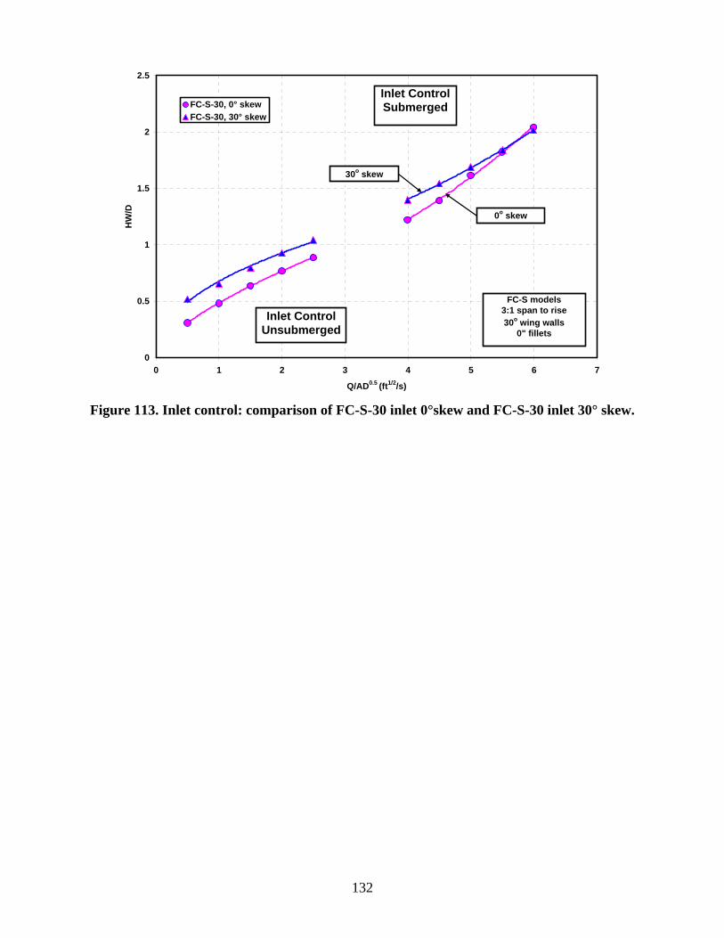
132

0

0.5

1

1.5

2

2.5

0 1 2 3 4 5 6 7

Q/AD0.5 (ft1/2/s)

HW

/D

FC-S-30, 0° skewFC-S-30, 30° skew



FC-S models3:1 span to rise30o wing walls

0" fillets

30o skew

0o skew

Figure 113. Inlet control: comparison of FC-S-30 inlet 0°skew and FC-S-30 inlet 30° skew.

133

APPENDIX C. SUMMARY OF REGRESSION COEFFICIENTS FOR ALL EXPERIMENTS

Tables 18, 19 and 20 of this appendix summarize the regression coefficients derived from all of the experiments conducted during this study. Table 18 lists the inlet-control design coefficients, K, M, c and Y which apply to the HDS-5 form 2 unsubmerged flow equation and the submerged flow equation as follows:

unsubmerged inlet-control form 2 equation

M

ui

ADQK

KD

HW⎥⎦⎤

⎢⎣⎡= 5.0 (18)

submerged inlet-control equation

S.YAD

QKcD

HW.

ui 702

50 ++⎥⎦⎤

⎢⎣⎡=

where: Ku = units conversion constant = 1.811 for SI units and 1.0 for customary English units.

Table 19 lists the inlet-control fifth-order polynomial constants a, b, c, d. e and f that are used by computer programmers to bridge the transition from unsubmerged to submerged flow and code the two equations as a continuous function. The fifth-order polynomial used in culvert design is as follows:

5

5.0

4

5.0

3

5.0

2

5.05.0 ⎥⎦⎤

⎢⎣⎡+⎥⎦

⎤⎢⎣⎡+⎥⎦

⎤⎢⎣⎡+⎥⎦

⎤⎢⎣⎡+⎥⎦

⎤⎢⎣⎡+=

ADQK

fAD

QKe

ADQK

dAD

QKc

ADQK

baD

HW uuuuui (19)

where: Ku = units conversion constant = 1.811 for SI units and 1.0 for customary English units.

Table 20 lists the outlet control loss coefficients Ke and Ko used to compute culvert entrance and culvert outlet losses are commonly expressed as functions of the barrel velocity head as follows

⎟⎟⎠

⎞⎜⎜⎝

⎛=

gVKH eLe 2

2

(20)

⎥⎥⎦

⎤

⎢⎢⎣

⎡⎟⎟⎠

⎞⎜⎜⎝

⎛−⎟⎟

⎠

⎞⎜⎜⎝

⎛=

gV

gVKH d

oLo 22

22

(21)

Where:

Ke = Entrance-loss coefficient;

134

Ko = Exit loss coefficient usually assumed to be 1.0 for design;

⎟⎟⎠

⎞⎜⎜⎝

⎛g

V2

2

= Velocity head inside the culvert barrel;

⎟⎟⎠

⎞⎜⎜⎝

⎛

gVd

2

2

= Velocity head in the downstream channel near the outlet; frequently neglected in design.

The downstream channel velocity for this study was taken as the average velocity in the tailbox using the full width of the tailbox multiplied by the average tail water depth as the flow area.

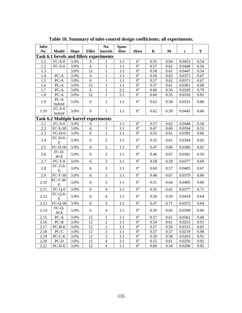
135

Table 18. Summary of inlet-control design coefficients; all experiments. Inlet No. Model Slope Fillet

No. barrels

Span: Rise Skew K M c Y

Task 6.1 bevels and fillets experiments 1.1 FC-S-0 3.0% 0 1 1:1 0o 0.55 0.64 0.0453 0.54 1.2 FC-S-0 3.0% 6 1 1:1 0o 0.57 0.62 0.0448 0.56 1.3 3.0% 12 1 1:1 0o 0.58 0.61 0.0447 0.54 1.4 PC-A 3.0% 0 1 1:1 0o 0.56 0.63 0.0371 0.67 1.5 PC-A 3.0% 6 1 1:1 0o 0.57 0.62 0.0371 0.67 1.6 PC-A 3.0% 12 1 1:1 0o 0.57 0.61 0.0361 0.68 1.7 PC-A 3.0% 6 1 2:1 0o 0.60 0.56 0.0329 0.79 1.8 PC-A 3.0% 12 1 2:1 0o 0.60 0.55 0.0316 0.81

1.9 PC-A hybrid 3.0% 0 1 1:1 0o 0.63 0.58 0.0331 0.80

1.10 FC-S-0 hybrid 3.0% 0 1 1:1 0o 0.62 0.59 0.0445 0.66

Task 6.2 Multiple barrel experiments 2.1 FC-S-0 3.0% 6 1 1:1 0o 0.57 0.62 0.0448 0.56 2.2 FC-S-30 3.0% 6 1 1:1 0o 0.47 0.69 0.0394 0.53 2.3 FC-D-0 3.0% 6 2 1:1 0o 0.55 0.61 0.0391 0.66

2.4 FC-D-0-E 3.0% 6 2 1:1 0o 0.55 0.61 0.0394 0.65

2.5 FC-D-30 3.0% 6 2 1:1 0o 0.47 0.66 0.0366 0.61

2.6 FC-D-30-E 3.0% 6 2 1:1 0o 0.46 0.67 0.0381 0.59

2.7 FC-T-0 3.0% 6 3 1:1 0o 0.58 0.58 0.0377 0.69

2.8 FC-T-0-E 3.0% 6 3 1:1 0o 0.60 0.57 0.0405 0.67

2.9 FC-T-30 3.0% 6 3 1:1 0o 0.48 0.67 0.0379 0.60

2.10 FC-T-30-E 3.0% 6 3 1:1 0o 0.51 0.64 0.0405 0.60

2.11 FC-Q-0 3.0% 6 4 1:1 0o 0.55 0.61 0.0377 0.71

2.12 FC-Q-0-E 3.0% 6 4 1:1 0o 0.58 0.59 0.0418 0.64

2.13 FC-Q-30 3.0% 6 4 1:1 0o 0.47 0.71 0.0372 0.64

2.14 FC-Q-30-E 3.0% 6 4 1:1 0o 0.50 0.65 0.0398 0.60

2.15 PC-A 3.0% 12 1 1:1 0o 0.57 0.61 0.0361 0.68 2.16 PC-B 3.0% 12 2 1:1 0o 0.54 0.61 0.0253 0.91 2.17 PC-B-E 3.0% 12 2 1:1 0o 0.57 0.58 0.0315 0.81 2.18 PC-C 3.0% 12 3 1:1 0o 0.57 0.57 0.0219 0.98 2.19 PC-C-E 3.0% 12 3 1:1 0o 0.59 0.58 0.0263 0.91 2.20 PC-D 3.0% 12 4 1:1 0o 0.55 0.61 0.0250 0.92 2.21 PC-D-E 3.0% 12 4 1:1 0o 0.60 0.54 0.0296 0.85

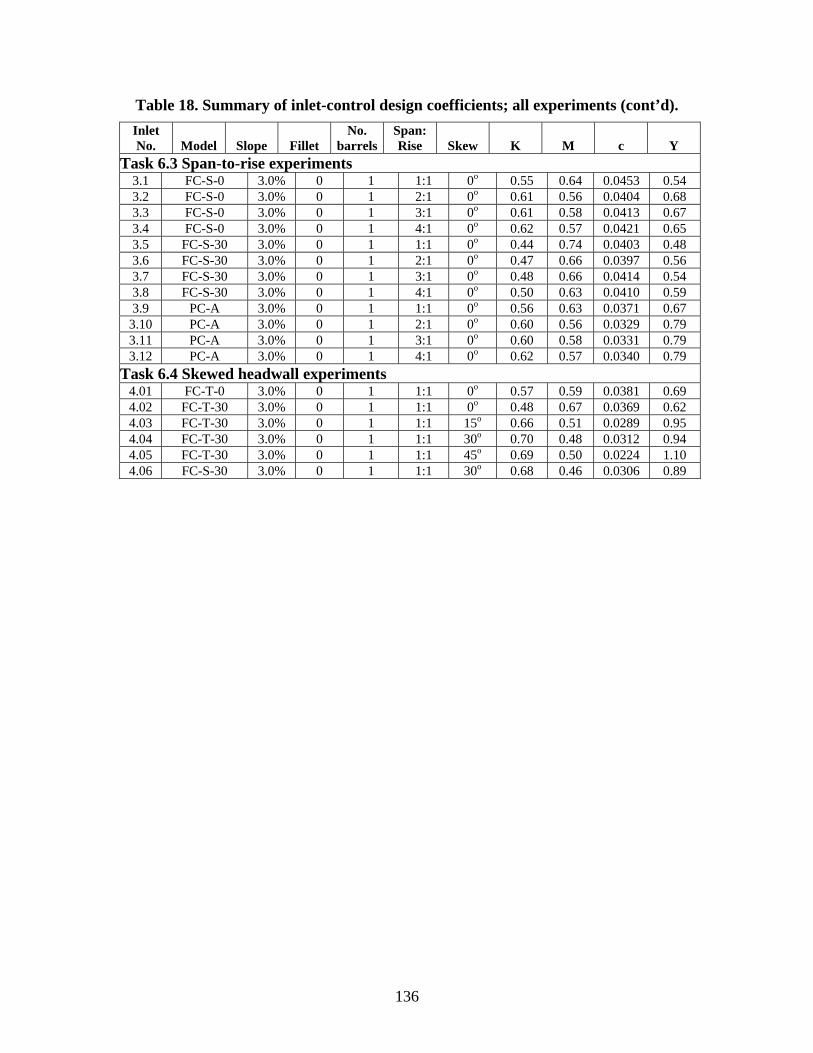
136

Table 18. Summary of inlet-control design coefficients; all experiments (cont’d). Inlet No. Model Slope Fillet

No. barrels

Span: Rise Skew K M c Y

Task 6.3 Span-to-rise experiments 3.1 FC-S-0 3.0% 0 1 1:1 0o 0.55 0.64 0.0453 0.54 3.2 FC-S-0 3.0% 0 1 2:1 0o 0.61 0.56 0.0404 0.68 3.3 FC-S-0 3.0% 0 1 3:1 0o 0.61 0.58 0.0413 0.67 3.4 FC-S-0 3.0% 0 1 4:1 0o 0.62 0.57 0.0421 0.65 3.5 FC-S-30 3.0% 0 1 1:1 0o 0.44 0.74 0.0403 0.48 3.6 FC-S-30 3.0% 0 1 2:1 0o 0.47 0.66 0.0397 0.56 3.7 FC-S-30 3.0% 0 1 3:1 0o 0.48 0.66 0.0414 0.54 3.8 FC-S-30 3.0% 0 1 4:1 0o 0.50 0.63 0.0410 0.59 3.9 PC-A 3.0% 0 1 1:1 0o 0.56 0.63 0.0371 0.67

3.10 PC-A 3.0% 0 1 2:1 0o 0.60 0.56 0.0329 0.79 3.11 PC-A 3.0% 0 1 3:1 0o 0.60 0.58 0.0331 0.79 3.12 PC-A 3.0% 0 1 4:1 0o 0.62 0.57 0.0340 0.79

Task 6.4 Skewed headwall experiments 4.01 FC-T-0 3.0% 0 1 1:1 0o 0.57 0.59 0.0381 0.69 4.02 FC-T-30 3.0% 0 1 1:1 0o 0.48 0.67 0.0369 0.62 4.03 FC-T-30 3.0% 0 1 1:1 15o 0.66 0.51 0.0289 0.95 4.04 FC-T-30 3.0% 0 1 1:1 30o 0.70 0.48 0.0312 0.94 4.05 FC-T-30 3.0% 0 1 1:1 45o 0.69 0.50 0.0224 1.10 4.06 FC-S-30 3.0% 0 1 1:1 30o 0.68 0.46 0.0306 0.89

137

Table 19. Summary of inlet-control fifth-order polynomial coefficients; all experiments.

Inlet No. Model Slope Fillet

No. barrels

Span: Rise Skew a b c d e f

Task 6.1 Bevels and fillets experiments 1.1 FC-S-0 3.0% 0 1 1:1 0o 0.2115 0.2243 0.2084 -0.1220 0.0247 -0.0016 1.2 FC-S-0 3.0% 6 1 1:1 0o 0.2245 0.2473 0.1865 -0.1135 0.0232 -0.0015 1.3 FC-S-0 3.0% 12 1 1:1 0o 0.2455 0.2182 0.2102 -0.1213 0.0241 -0.0015 1.4 PC-A 3.0% 0 1 1:1 0o 0.1942 0.3107 0.1094 -0.0774 0.0162 -0.0011 1.5 PC-A 3.0% 6 1 1:1 0o 0.2031 0.3135 0.1077 -0.0769 0.0160 -0.0010 1.6 PC-A 3.0% 12 1 1:1 0o 0.2106 0.3146 0.1020 -0.0727 0.0149 -0.0010 1.7 PC-A 3.0% 6 1 2:1 0o 0.1868 0.4823 -0.0704 -0.0031 0.0032 -0.0003 1.8 PC-A 3.0% 12 1 2:1 0o 0.1892 0.4968 -0.0908 0.0059 0.0015 -0.0002

1.9 FC-S-0 hybrid 3.0% 0 1 1:1 0o -0.0017 0.0245 -0.1148 0.1673 0.3073 0.2405

1.10 PC-A hybrid 3.0% 0 1 1:1 0o -0.0030 0.0446 -0.2230 0.4287 0.0327 0.3250 Task 6.2 Multiple barrel experiments

2.1 FC-S-0 3.0% 6 1 1:1 0o 0.2245 0.2473 0.1865 -0.1135 0.0232 -0.0015 2.2 FC-S-30 3.0% 6 1 1:1 0o 0.1490 0.2504 0.1293 -0.0804 0.0165 -0.0011 2.3 FC-D-0 3.0% 6 2 1:1 0o 0.1547 0.4366 -0.0343 -0.0175 0.0060 -0.0004 2.4 FC-D-0-E 3.0% 6 2 1:1 0o 0.1685 0.4065 -0.0009 -0.0318 0.0085 -0.0006 2.5 FC-D-30 3.0% 6 2 1:1 0o 0.1010 0.4192 -0.0551 -0.0027 0.0029 -0.0002 2.6 FC-D-30-E 3.0% 6 2 1:1 0o 0.1037 0.4021 -0.0360 -0.0111 0.0045 -0.0003 2.7 FC-T-0 3.0% 6 3 1:1 0o 0.1856 0.4259 -0.0151 -0.0274 0.0078 -0.0006 2.8 FC-T-0-E 3.0% 6 3 1:1 0o 0.2205 0.3704 0.0571 -0.0600 0.0138 -0.0009 2.9 FC-T-30 3.0% 6 3 1:1 0o 0.1325 0.3409 0.0427 -0.0443 0.0101 -0.0007

2.10 FC-T-30-E 3.0% 6 3 1:1 0o 0.1465 0.3699 0.0183 -0.0372 0.0093 -0.0006 2.11 FC-Q-0 3.0% 6 4 1:1 0o 0.1542 0.4484 -0.0407 -0.0141 0.0052 -0.0004 2.12 FC-Q-0-E 3.0% 6 4 1:1 0o 0.2026 0.3694 0.0563 -0.0592 0.0137 -0.0009 2.13 FC-Q-30 3.0% 6 4 1:1 0o 0.1084 0.3555 0.0273 -0.0343 0.0079 -0.0005 2.14 FC-Q-30-E 3.0% 6 4 1:1 0o 0.1449 0.3501 0.0414 -0.0461 0.0108 -0.0007

139

Table 19. Summary of inlet-control fifth-order polynomial coefficients; all experiments (cont’d). Inlet No. Model Slope Fillet

No. barrels

Span: Rise Skew a b c d e f

2.15 PC-A 3.0% 12 1 1:1 0o 0.2106 0.3146 0.1020 -0.0727 0.0149 -0.0010 2.16 PC-B 3.0% 12 2 1:1 0o 0.0993 0.6079 -0.2216 0.0668 -0.0098 0.0006 2.17 PC-B-E 3.0% 12 2 1:1 0o 0.1494 0.5404 -0.1423 0.0290 -0.0026 0.0001 2.18 PC-C 3.0% 12 3 1:1 0o 0.1473 0.5456 -0.1462 0.0322 -0.0035 0.0002 2.19 PC-C-E 3.0% 12 3 1:1 0o 0.1533 0.5558 -0.1521 0.0351 -0.0042 0.0002 2.20 PC-D 3.0% 12 4 1:1 0o 0.1070 0.6005 -0.2075 0.0609 -0.0089 0.0005 2.21 PC-D-E 3.0% 12 4 1:1 0o 0.1589 0.5859 -0.1918 0.0485 -0.0059 0.0003

Task 6.3 Span-to-rise experiments 3.1 FC-S-0 3.0% 0 1 1:1 0o 0.2115 0.2243 0.2084 -0.1220 0.0247 -0.0016 3.2 FC-S-0 3.0% 0 1 2:1 0o 0.2072 0.4321 -0.0118 -0.0323 0.0092 -0.0007 3.3 FC-S-0 3.0% 0 1 3:1 0o 0.2272 0.3614 0.0770 -0.0700 0.0157 -0.0011 3.4 FC-S-0 3.0% 0 1 4:1 0o 0.2466 0.3158 0.1261 -0.0914 0.0196 -0.0013 3.5 FC-S-30 3.0% 0 1 1:1 0o 0.1635 0.1271 0.2562 -0.1316 0.0252 -0.0016 3.6 FC-S-30 3.0% 0 1 2:1 0o 0.1147 0.3769 -0.0074 -0.0243 0.0070 -0.0005 3.7 FC-S-30 3.0% 0 1 3:1 0o 0.1415 0.3213 0.0641 -0.0561 0.0127 -0.0009 3.8 FC-S-30 3.0% 0 1 4:1 0o 0.2466 0.3158 0.1261 -0.0914 0.0196 -0.0013 3.9 PC-A 3.0% 0 1 1:1 0o 0.1942 0.3107 0.1094 -0.0774 0.0162 -0.0011

3.10 PC-A 3.0% 0 1 2:1 0o 0.1547 0.5928 -0.1901 0.0486 -0.0064 0.0004 3.11 PC-A 3.0% 0 1 3:1 0o 0.2007 0.4245 0.0003 -0.0329 0.0083 -0.0006 3.12 PC-A 3.0% 0 1 4:1 0o 0.2200 0.4040 0.0294 -0.0466 0.0109 -0.0007

Task 6.4 Skewed headwall experiments 4.1 FC-T-0 3.0% 0 3 1:1 0o 0.1834 0.4091 0.0056 -0.0358 0.0093 -0.0007 4.2 FC-T-30 3.0% 0 3 1:1 0o 0.1284 0.3550 0.0267 -0.0375 0.0089 -0.0006 4.3 FC-T-30 3.0% 0 3 1:1 15o 0.1820 0.6863 -0.2770 0.0821 -0.0117 0.0007 4.4 FC-T-30 3.0% 0 3 1:1 30o 0.2260 0.6584 -0.2403 0.0634 -0.0080 0.0004 4.5 FC-T-30 3.0% 0 1 1:1 45o 0.1875 0.7437 -0.3236 0.1036 -0.0161 0.0010 4.6 FC-S-30 3.0% 0 1 1:1 30o 0.2131 0.6855 -0.2982 0.0886 -0.0122 0.0007

141

Table 20. Summary of outlet-control design coefficients; all experiments.

Inlet No. Model Slope Fillet No.

barrels Span: Rise Skew

Outlet loss Ko

unsubmerged

Outlet loss Ko

submerged

Entrance lossKe

unsubmerged

Entrance loss Ke

submerged

Task 6.1 bevels and fillets experiments 1.1 FC-S-0 3.0% 0 1 1:1 0o NA 1.22 NA 0.45 1.2 FC-S-0 3.0% 6 1 1:1 0o NA 1.25 NA 0.47 1.3 FC-S-0 3.0% 12 1 1:1 0o NA 1.17 NA 0.64 1.4 PC-A 3.0% 0 1 1:1 0o NA 1.22 NA 0.25 1.5 PC-A 3.0% 6 1 1:1 0o NA 1.18 NA 0.23 1.6 PC-A 3.0% 12 1 1:1 0o NA 1.19 NA 0.30 1.7 PC-A 3.0% 6 1 2:1 0o NA 1.25 NA 0.35 1.8 PC-A 3.0% 12 1 2:1 0o NA 0.98 NA 0.40 1.1 FC-S-0 0.7% 0 1 1:1 0o 1.03 1.17 0.73 0.46 1.2 FC-S-0 0.7% 6 1 1:1 0o 0.87 1.12 0.90 0.50 1.3 FC-S-0 0.7% 12 1 1:1 0o 1.10 1.13 0.90 0.62 1.4 PC-A 0.7% 0 1 1:1 0o 1.07 1.19 0.67 0.27 1.5 PC-A 0.7% 6 1 1:1 0o 1.28 1.30 0.63 0.25 1.6 PC-A 0.7% 12 1 1:1 0o 1.10 1.14 0.56 0.33

Task 6.2 Multiple barrel experiments 2.1 FC-S-0 0.7% 6 1 1:1 0o 0.87 1.12 0.90 0.50 2.2 FC-S-30 0.7% 6 1 1:1 0o 1.07 1.16 0.71 0.26 2.3 FC-D-0 0.7% 6 2 1:1 0o 0.84 1.07 0.71 0.52

2.4 FC-D-0-

E 0.7% 6 2 1:1 0o 0.86 1.09 0.32 0.53 2.5 FC-D-30 0.7% 6 2 1:1 0o 0.76 1.03 0.74 0.34

2.6 FC-D-30-E 0.7% 6 2 1:1 0o 0.90 1.09 0.42 0.31

2.7 FC-T-0 0.7% 6 3 1:1 0o 1.00 0.91 0.60 0.54

2.8 FC-T-0-

E 0.7% 6 3 1:1 0o 0.90 0.93 0.80 0.58

143

Table 20. Summary of outlet-control design coefficients; all experiments (cont’d).



Outlet loss Ko

unsubmerged

Outlet loss Ko

submerged

Entrance lossKe

unsubmerged

Entrance loss Ke

submerged 2.9 FC-T-30 0.7% 6 3 1:1 0o 1.00 1.05 0.48 0.31

2.10 FC-T-30-E 0.7% 6 3 1:1 0o 1.09 1.26 0.41 0.32

2.11 FC-Q-0 0.7% 6 4 1:1 0o 1.23 1.09 0.83 0.52

2.12 FC-Q-0-

E 0.7% 6 4 1:1 0o 1.08 1.16 0.87 0.50

2.13 FC-Q-

30 0.7% 6 4 1:1 0o 0.86 1.08 0.38 0.32

2.14 FC-Q-30-E 0.7% 6 4 1:1 0o 0.89 1.05 0.38 0.34

2.15 PC-A 0.7% 12 1 1:1 0o 1.10 1.14 0.56 0.33 2.16 PC-B 0.7% 12 2 1:1 0o 0.79 1.00 0.96 0.49 2.17 PC-B-E 0.7% 12 2 1:1 0o 0.96 1.08 0.75 0.56 2.18 PC-C 0.7% 12 3 1:1 0o 1.01 1.25 0.94 0.54 2.19 PC-C-E 0.7% 12 3 1:1 0o 1.21 1.14 0.96 0.51 2.20 PC-D 0.7% 12 4 1:1 0o 1.05 0.98 0.91 0.59 2.21 PC-D-E 0.7% 12 4 1:1 0o 1.07 1.05 0.93 0.58 Task 6.3 Span-to-rise experiments

3.1 FC-S-0 0.7% 0 1 1:1 0o 1.03 1.17 0.73 0.46 3.2 FC-S-0 0.7% 0 1 2:1 0o 0.87 1.02 0.48 0.40 3.3 FC-S-0 0.7% 0 1 3:1 0o 1.20 1.45 0.66 0.32 3.4 FC-S-0 0.7% 0 1 4:1 0o 1.07 1.16 0.62 0.40 3.5 FC-S-30 0.7% 0 1 1:1 0o 0.75 1.12 0.39 0.27 3.6 FC-S-30 0.7% 0 1 2:1 0o 0.97 1.07 0.39 0.22

145

Table 20. Summary of outlet-control design coefficients; all experiments (cont’d).



Outlet loss Ko

unsubmerged

Outlet lossKo

submerged

Entrance lossKe

unsubmerged

Entrance lossKe

submerged 3.7 FC-S-30 0.7% 0 1 3:1 0o 1.49 1.27 0.48 0.19 3.8 FC-S-30 0.7% 0 1 4:1 0o 0.87 1.14 0.53 0.18 3.9 PC-A 0.7% 0 1 1:1 0o 1.07 1.19 0.67 0.27

3.10 PC-A 0.7% 0 1 2:1 0o 0.92 1.09 0.42 0.34 3.11 PC-A 0.7% 0 1 3:1 0o 1.76 1.52 0.80 0.29 3.12 PC-A 0.7% 0 1 4:1 0o 0.95 1.15 0.69 0.26

Task 6.4 Skewed headwall experiments 4.1 FC-T-0 0.7% 0 1 1:1 0o 1.31 1.32 0.84 0.39 4.2 FC-T-30 0.7% 0 1 1:1 0o 0.86 0.98 0.47 0.35 4.3 FC-T-30 0.7% 0 1 1:1 15o 0.88 1.13 0.86 0.47 4.4 FC-T-30 0.7% 0 1 1:1 30o 0.94 1.00 0.43 0.36 4.5 FC-T-30 0.7% 0 1 1:1 45o 0.95 0.97 0.85 0.44 4.6 FC-S-30 0.7% 0 1 1:1 30o 0.84 1.03 0.9 0.46

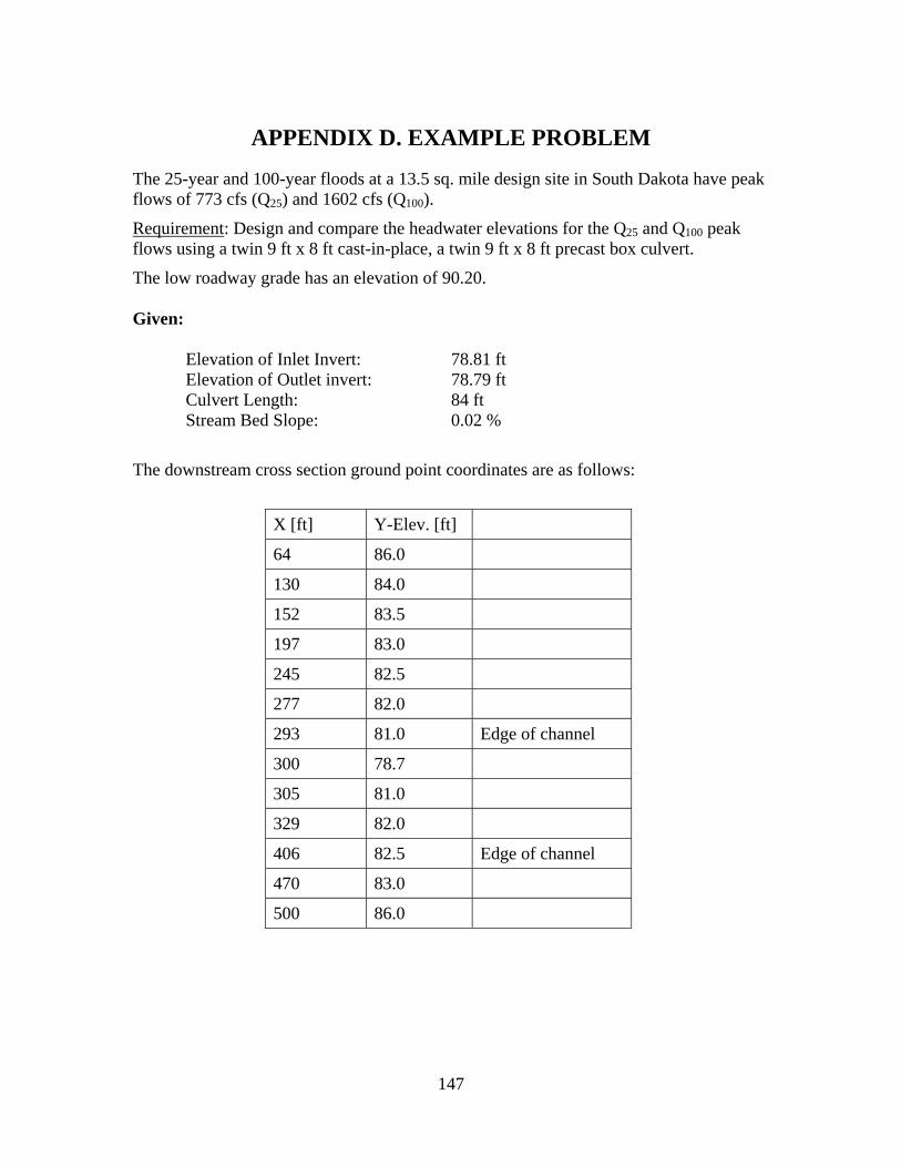
147

APPENDIX D. EXAMPLE PROBLEM

The 25-year and 100-year floods at a 13.5 sq. mile design site in South Dakota have peak flows of 773 cfs (Q25) and 1602 cfs (Q100).

Requirement: Design and compare the headwater elevations for the Q25 and Q100 peak flows using a twin 9 ft x 8 ft cast-in-place, a twin 9 ft x 8 ft precast box culvert.

The low roadway grade has an elevation of 90.20. Given:

Elevation of Inlet Invert: 78.81 ft Elevation of Outlet invert: 78.79 ft Culvert Length: 84 ft Stream Bed Slope: 0.02 %

The downstream cross section ground point coordinates are as follows:

X [ft] Y-Elev. [ft]

64 86.0

130 84.0

152 83.5

197 83.0

245 82.5

277 82.0

293 81.0 Edge of channel

300 78.7

305 81.0

329 82.0

406 82.5 Edge of channel

470 83.0

500 86.0

148

The tailwater rating information is as follows:

Flow [cfs] T.W. Elev. [ft]

68.7 82.77

222.0 83.49

375.4 83.93

528.7 84.30

682.0 84.61

773.0 84.78

988.7 85.15

1142.0 85.38

1295.3 85.61

1448.7 85.82

1602.0 86.00 STEP 1: Plot the downstream discharge rating curve and flow area curves based on

ground point coordinates.

149

0

200

400

600

800

1000

1200

1400

1600

1800

82.5 83 83.5 84 84.5 85 85.5 86 86.5Tail water elevation [ft]

Dis

char

ge [c

fs]

Q100

Q25

84.7

8 ft

86 ft773 cfs

1602 cfs

Figure 114. Discharge – tailwater (T.W.) variation.

Figure 115. Downstream cross section.

150

0

200

400

600

800

1000

1200

1400

82.5 83 83.5 84 84.5 85 85.5 86 86.5Tail water elevation [ft]

Flow

are

a [ft

2 ]

86 ft

84.7

8 ft

Q25: A = 810.88 ft2

A = 26.107 x (TWelev)2 - 4044.9 x TWelev + 156088

Q100: A = 1310.80 ft2

Figure 116. Cross section area vs. tailwater elevation.

Based on regression of the area versus tail water elevation curve in figure 116, the downstream flow area for a tailwater elevation is:

088,156TWelev9.4044)TWelev(107.26A 2 +×−×= (22)

Assuming the upstream section is a vertical shift of the downstream section according to the 0.02 percent channel slope, the flow area under the headwater elevation can be computed by substituting HWelev – 84 × 0.02 percent for the TWelev in the above equation to yield:

95.156155HWelev777.4045)HWelev(107.26A 2 +×−×= (23)

STEP 2: Compute downstream channel velocity.

VTW = Q / A = 773 / 810.88 = 0.95 ft/sec for Q25 (24)

VTW = Q / A = 1602 / 1310.80 = 1.22 ft/sec for Q100 (25)

151

STEP 3: Compute critical depth using equation 26. At critical flow NF = V/(g × ym)1/2 = 1, but V = Q / A and A = B × dc – NB × a2

Where:

ym = mean hydraulic depth = A / B = (B × dc – NB × a2) / B

B = total culvert width = NB × span of each barrel

dc = flow depth measured from the invert

a = corner fillet height = 0.5 ft for the FC culvert or 1.0 ft for the PC culvert

NB = number of barrels

BaNB)g/BQ(d

22

c

31

×+×= (26)

The above equation applies if the critical depth is below the top corner fillets. If the critical depth does partially submerge the top fillets the relationship becomes:

B)aa(NB)g/)aNB2B(Q(d

2t

2t

2

c

31

+×+××−×= (26a)

Where:

at = Submergence of top corner fillets = dc – (D − a)

Solving this equation would be a trial and error procedure, but can be solved using the goal seek tool of EXCEL.

Culvert a dc for Q25 dc for Q100

Critical depth elev at outlet for

Q25 (ft)

Critical depth elev at outlet for

Q100(ft) FC-D-30 9’x 8’ 6-inch 3.88 ft 6.29 ft 82.67 ft 85.09 ft

FC-D-0 9’x 8’ 6-inch 3.88 ft 6.29 ft 82.67 ft 85.09 ft

PC-B 9’ x 8’ 12-inch 3.96 ft 6.37 ft 82.75 ft 85.16 ft

PC-B 9’ x 8’ 0-inch 3.86 ft 6.26 ft 82.65 ft 85.05 ft

152

STEP 4: Determine normal depths in the culvert from Manning’s equation.

2/1o

3/2H SRA

n49.1Q = (27)

Where:

The flow area, A, and the hydraulic radius, RH, can be computed from the equations below if the normal depth is below the top corner fillets.

A = NB × (span × dn − a2)

RH = A / NB × (span + 2 × dn − 1.17 × a)

The flow area, A, and the hydraulic radius, RH, can be computed from the equations below if the normal depth partially submerges the top corner fillets.

A = NB × (span × dn − (a2 + at2))

RH = A / NB × (span + 2 × dn − 1.17 × a + 0.848 x at2)

Where:

at = Submergence of top corner fillets = dn – (D − a)

If the normal depth exceeds the rise, D, of the culvert, set at equal to a and compute the normal depth that would occur if the culvert did not have a crown.

The normal depth can be determined by trial and error or by using the goal seek tool from Excel.

Culvert a dn for Q25 dn for Q100

FC-D-30 9’ x 8’ 6-inch 10.49 ft 19.61 ft

FC-D-0 9’ x 8’ 6-inch 10.49 ft 19.61 ft

PC-B 9’ x 8’ 12-inch 10.69 ft 19.82 ft

PC-B 9’ x 8’ 0-inch 10.44 ft 19.57 ft

153

STEP 5: Determine initial depth do at barrel exit to start backwater calculation.

The normal depths are greater than critical depths; therefore the culverts will be outlet control whether or not the barrels flow full at the inlet. The TW elevations are greater than the critical depth elevations and are below the crown elevations at the outlet; therefore the depth at the culvert outlet will be between the critical depth and the culvert crown and can be computed from equation 28 below.

⎟⎟⎠

⎞⎜⎜⎝

⎛−+−+=+

g2V

g2V

K.ElevInvertg2

V.ElevTW

g2V

d2TW

2o

o

2TW

2o

o (28)

Assume Ko = 1.0 (see HDS-5 p. 35).

The outlet is unsubmerged and the footnote below table 7 of the research report warns that the unsubmerged Ko values are unreliable, but the unsubmerged value for a twin box culvert happens to be the traditional value that is recommended for the outlet loss. The exit coefficients derived for this study neglects the tailwater velocity head.

.ElevInvert.ElevTWd0.1Kfor oo −=→= (29)

Figure 117. Definition sketch for exit loss.

do = TW Elev − Invert Elev at outlet = TW Elev − 78.79 (30)

154

Culvert

TW HGL Elev for

Q25 (ft)

do for Q25 (ft)

EGL Elev at culvert

outlet for Q25 (ft)

TW HGL

Elev for Q100 (ft)

do for Q100 (ft)

EGL Elev at culvert outlet

for Q100 (ft)

FC – D-30 9’ x 8’

84.78 5.99 85.58 86.00 7.21 88.38

PC-B 9’ x 8’

84.78 5.99 85.61 86.00 7.21 88.46

STEP 6: Use standard step backwater calculations to determine the EGL in the culvert

for free surface flow. This can be done fairly easily on a spreadsheet by incrementing the depth between do at the outlet and the full culvert depth, D. Compute ΔL from equation 31 below and L=Σ (ΔL) after each step; then compare L with the length of the culvert (84 ft) to determine where computations are complete. Since the corner fillets affect the backwater computations, develop the spreadsheet in two stages.

For d < D − a, use Δd = [(D − a) − do] / 1000; take1000 steps in the spreadsheet

di = di-1 + Δd

Ai = NB × (span × di – a2)

Rh i = Ai / NB × (span + 2 × di – 1.17 × a]

For D > d > D − a, use Δd = a / 20, take 19 steps in the spreadsheet

di = di-1 + Δd

at i = di – (D – a)

Ai = NB × (span × di – (a2 + at i2)

Rh i = Ai / (NB × (span + 2 × di − 1.17 × a +0.848 × at i))

For d = D, the last step di = D

Ai = NB × (span × D – 2 × a2)

Rh i = Ai / (NB × (2 × span + 2 × D – 2.34 × a))

155

Where: subscript “i” is a line in the step-backwater computation.

The average area and hydraulic radius for any step in the step-backwater are:

Am = (Ai + Ai+1)/2

RHm = (RHi +RHi+1)/2

The friction slope, SF, for any step is computed from Manning’s equation.

2

32mm

F RA5.1QnS ⎟⎟

⎠

⎞⎜⎜⎝

⎛= (31)

The step length is then computed from the energy balance.

Fb

21i1i

2ii

SS)g2/Vd()g2/Vd(L

−+−+

=Δ ++ (32)

Where:

span = width of one barrel [ft]

D = rise of the culvert [ft]

d = flow depth in barrel, [ft]

at = partially submerged top fillet

V = flow velocity in barrel, [ft/s]

SF = friction slope or energy slope

Sb = barrel slope

Q = discharge, [cfs]

n = Manning roughness coefficient; n = 0.012, [ft-1/3]

If the culvert fills to the crown before the computations reach the entrance, the EGL at the entrance is:

g2V

RLn29

g2V

DEGL2FULL

3/4FULLh

FULL22

FULLUS ×

⎥⎥⎦

⎤

⎢⎢⎣

⎡++=

(33)

156

Where:

VFULL = Q / AFULL

AFULL = NB × (span × D – a2)

RhFULL = ))a343.2D2span(NB(/AFULL ×−×+×

LFULL = length of culvert flowing full

STEP 7: Determine entrance loss. HGL is greater then critical depth throughout the

barrel indicating outlet control. Use table 1 or table 12 to find entrance loss coefficients.

Inlet Ke

Sketch 2 30o flared wing-walls, top edge beveled at 45o, 2, 3 and 4 multiple barrels (FC-D-30)

0.32

Sketch 8 0o flared wing-walls (extension of sides), 45o straight bevel at crown, 2, 3 and 4 multiple barrels (FC-D-0)

0.52

Sketch 12 0o flared wing-walls (extension of sides), crown rounded at 8” radius, w/ 12” corner fillets, 2, 3 and 4 multiple barrels PC-B

0.54

g2V

Kh2US

eeL ×= (34)

where: VUS = velocity at the upstream end of the culvert from the step backwater or the full flow computations.

157

STEP 8: Compute headwater elevation.

HWEGL = EGL elevUS + hLe

Where: EGL elevUS is the EGL elev at the upstream end of the culvert from the backwater calculations.

The HWEGL’s are energy grade line elevations and include the velocity head, which is usually negligible in the headwater pool. To get the actual water-surface elevations, HWHGL in the headwater pool, use the following relationships:

A/Qg2

Vwhere,

g2V

HWHW2HW

2HW

HGLEGL =+= (35)

with 95.156155HWelev777.4045)HWelev(107.26A 2 +×−×= (Equation 23)

The water surface elevation, HWelev, in the headwater pool can be determined by trial and error or by using the goal seek tool of EXCEL.

Tables 21 and 22 below summarize the results of the step backwater computations, the headwater EGL computations and the headwater HGL computations.

Table 21. Results from step backwater and entrance loss computations for Q25.

Culvert Span x Rise

Fillet Size

HGL ElevUS

(ft)

EGL ElevUS

(ft) Ke

HWEGL

(ft)

Area in HW Pool (ft2)

Velocity in HW Pool (ft/s)

Water Surface Elev. HWelev

(ft)

FC-D-30 9’ x 8’ 6” 84.877 85.662 0.32 85.913 1265 0.65 85.907

FC-D-0 9’ x 8’ 6” 84.877 85.662 0.52 86.071 1335 0.58 86.065

PC-B 9’ x 8’ 12” 84.879 85.686 0.54 86.121 1358 0.57 86.116

PC-B 9’ x 8’ 0” 84.879 85.656 0.54 86.076 1228 0.63 85.823

158

Table 22. Results from step backwater and entrance loss computations for Q100.

Culvert Span x Rise

Fillet Size

HGL ElevUS

(ft)

EGL ElevUS

(ft) Ke

HWEGL

(ft)

Area in HW Pool (ft2)

Velocity in HW Pool (ft/s)

Water Surface Elev. HWelev

(ft)

FC-D-30 9’ x 8’ 6” 86.458 88.578 0.32 89.256 3028 0.53 89.251

FC-D-0 9’ x 8’ 6” 86.458 88.578 0.52 89.680 3294 0.48 89.676

PC-B 9’ x 8’ 12” 86.471 88.657 0.54 89.837 3394 0.47 89.834

PC-B 9’ x 8’ 0” 86.463 88.563 0.54 89.697 3305 0.48 89.693

Results of the step backwater and entrance loss computations for the Q100 discharge only are illustrated in the sketches for the five culvert configurations in figures 118 through 121 below.

159

Figure 118. Field cast, twin 9’ x 8’, 30° WW, culvert sketches with Q100 elevations.

160

Figure 119. Field cast, twin 9’ x 8’, 0° WW, culvert sketches with Q100 elevations.

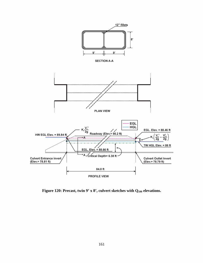
161

Figure 120: Precast, twin 9’ x 8’, culvert sketches with Q100 elevations.

162

Figure 121. Precast, twin 9’ x 8’, zero fillets, culvert sketches with Q100 elevations.

163

SUMMARY

This example is included to illustrate how to apply the entrance loss coefficients from the laboratory results. The SD DOT provided site data and culvert options. We divided the example into eight basic steps for spreadsheet computations since there was not a design program to account for the corner fillets, which were a consideration in the laboratory study.

The first step was to plot the channel cross-section and derive expressions for channel area versus water surface elevations. The tailwater channel velocities and energy grade line elevations, EGL’s, were then computed from the downstream rating data that was provided. The critical depth and normal depth in the culvert were computed to determine if inlet control was a possibility. The normal depth computation is a tedious trial and error process especially when the corner fillets are included in the computation, but the goal seek tool from excel makes that an easy task. Inlet control was not a possibility because normal depths were greater than critical depths. The brink depth at the culvert outlet was computed from the following set of equations:

g2VEGLd

2o

oo −=

LoTWo hEGLEGL +=

)g2

Vg2

V(Kh2TW

2o

oLo −=

widthculverttotaldQV

oo ×

=

Where:

Ko is the outlet loss coefficient. We assumed Ko = 1.0

Since the brink depth was below the crown of the culvert, a spreadsheet was developed for step backwater computations through the culvert by incrementing the depth and computing the corresponding step length. Spreadsheets were analyzed to determine where either the cumulative step lengths equaled the culvert length or the culvert flowed full. None of the culverts flowed full for either Q25 or Q100 before the cumulative step lengths equaled the culvert length (84’); so free surface flow occurred in each case. The velocity and energy grade line elevation at the upstream end of the culvert from the step backwater computations were used to compute the headwater energy grade line elevation from the following equation:

g2VKEGLHW

2US

eUSEGL +=

164

Where:

EGLUS and VUS are energy grade line elevation and velocity at the upstream end of the culvert from the step backwater computations.

Ke = entrance loss coefficient from the laboratory results. We assumed Ke = 0.32 for the field cast inlet with 30o wing walls Ke = 0.52 for the field cast inlet with 0o wing walls and Ke = 0.54 for the precast inlet.

Last, the hydraulic grade line elevation (water surface elevation) was computed by subtracting the velocity head in the headwater pool from the energy grade line elevation. Again this was a trial and error computation because of the irregular channel geometry but was done by the goal seek tool. There was very little difference between the energy grade line and water surface elevations in the headwater pool.

The net area (with area of fillets removed) was used for the step backwater computations and for velocity computations. The research showed that the coefficients were not affected by the fillet sizes tested as long as the net area was used in the computations. Figure 122 is a sketch showing the procedure for calculating the net area. The current version of FHWA’s HY-8 program does not account for corner fillets.

We computed the headwater elevation for the PC-B, 9’ x 8’culverts with zero fillets to show the sensitivity of including or not including the corner fillets. The error by not accounting for the 12-inch fillets was more than 0.10 ft for the Q100 discharge. These errors would increase as the size of the culvert decreases and will decrease as the size of the culvert increases. The current version of HY-8 does not have a way to account for corner fillets. A design program such as HY-8 could certainly account for the corner fillets but it would add significant coding to the program

The HW elevations for the precast culverts were approximately 0.6 ft higher than the elevations for the field-cast culverts with the 30-degree wing walls at the Q100 discharge.

Figure 122. Sketch showing the net area used for the backwater computations.

165

APPENDIX E. REFERENCES

1. Normann, Jerome M., Robert J. Houghtalen and William J. Johnston,

“Hydraulic Design of Highway Culverts,” Federal Highway Administration Hydraulic Design Series No. 5 (HDS-5), Report number FHWA-IP-85-15, Washington, D.C., Sept 1985.

2. French, John L., “Hydraulics of Short Pipes, Hydraulic Characteristics of Commonly Used Pipe Entrances, First Progress Report,” NBS Report No. 4444, National Bureau of Standards, Washington, D.C., December 1955.

3. French, John L., “Hydraulics of Culverts, Second Progress Report, Pressure and Resistance Characteristics of a Model Pipe Culvert,” NBS Report No. 4911, National Bureau of Standards, Washington, D.C., Oct. 1956.

4. French, John L., “Hydraulics of Culverts, Third Progress Report, Effects of Approach Channel Characteristics on Model Pipe Culvert Operation,” NBS Report No. 5306, National Bureau of Standards, Washington, D.C., June 1957.

5. French, John L., “Hydraulics of Improved Inlet Structures for Pipe Culverts, Fourth Progress Report, Pressure and Resistance Characteristics of a Model Pipe Culvert,” NBS Report No. 7178, National Bureau of Standards, Washington, D.C., Aug. 1961.

6. French, John L., “Hydraulics of Culverts, Fifth Progress Report, Nonenlarged Box Culvert Inlets,” NBS Report No. 9327, National Bureau of Standards, Washington, D.C., June 1966.

7. French, John L., “Hydraulics of Culverts, Sixth Progress Report, Tapered Box Culvert Inlets,” NBS Report No. 9355, National Bureau of Standards, Washington, D.C., June 1966.

8. French, John L. and Herbert G. Bossy, “Hydraulics of Culverts, Seventh Progress Report, Tapered Box Inlets with Fall Concentration in the Inlet Structure,” NBS Report No. 9528, National Bureau of Standards, Washington, D.C., July 1967.

9. Graziano, Frank, Stuart Stein, Ed Umbrell and Brett Martin, “Determination of Single Barrel Box Culvert Inlet Loss Coefficients” published by SD DOT as Report SD1993-12, prepared by GKY& Associates, Inc., for the Federal Highway Administration, McLean, VA, June 2001.

10. McEnroe, Bruce M. and Lance M. Johnson, “Hydraulics of Flared End Sections for Pipe Culverts,” Transportation Research Record 1483, Transportation Research Board, National Academy Press, Washington, D.C., 1995.

11. Graziano, Frank, Stuart Stein, Ed Umbrell and Brett Martin, “Hydraulics of Slope Tapered Pipe Culverts,” Report FHWA-RD-01-077, prepared by

166

GKY& Associates, Inc., for Federal Highway Administration, McLean, VA, June 2001.

12. Jones, J. Sterling, Mark P. Mistichelli and Roger T. Kilgore “Long Span and Special Shape Culverts,” unpublished lab report FHWA-RD-91-085, Federal Highway administration, Turner Fairbank Highway Research Center, McLean, VA, June 1991.

13. Tullis, Blake, personal communication, Aug. 2004.

14. Umbrell, Edward, Ken Young, Christine Estes, Stuart M. Stein and David R. Pearson, “Hydraulics of Dale Boulevard Culverts: Performance Curve for a Prototype of Two Large Culverts in Series,” unpublished FHWA Report FHWA-RD-01-095, prepared by GKY& Associates, Inc., for Federal Highway Administration, McLean, VA, 2001.

15. GKY and Associates, “Compilation of Culvert Design Coefficients,” unpublished lab report, prepared by GKY& Associates, Inc. for Federal Highway Administration, McLean, VA, October 1998.

Documents

Effects of Inlet Geometry on Hydraulic Performance of …sddot.com/business/research/projects/docs/SD2002_04_Final_Report.pdfDesign coefficients are recommended for several ... Effects