Embed Size (px)
Citation preview

EFFECTS OF FIXED POINT FFT IMPLEMENTATION
ON WIRELESS LAN
A THESIS SUBMITTED IN PARTIAL FULFILLMENT
OF THE REQUIREMENTS FOR THE DEGREE OF
Master of Technology In
VLSI Design & Embedded System
By
GOVINDA MUTYALA RAO.T Roll No: 20507009
Department of Electronics & Communication Engineering
National Institute of Technology
Rourkela
2007

EFFECTS OF FIXED POINT FFT IMPLEMENTATION
ON WIRELESS LAN
A THESIS SUBMITTED IN PARTIAL FULFILLMENT
OF THE REQUIREMENTS FOR THE DEGREE OF
Master of Technology In
VLSI Design & Embedded system
By
GOVINDA MUTYALA RAO.T Roll No: 20507009
Under the guidance of
Prof.S.K.PATRA
Department of Electronics & Communication Engineering
National Institute of Technology
Rourkela
2007

National Institute of Technology
Rourkela
CERTIFICATE
This is to certify that the Thesis Report entitled “Effects of fixed point FFT implementation
on wireless LAN” submitted by Mr. Govinda Mutyala Rao.T (20507009) in partial
fulfillment of the requirements for the award of Master of Technology degree in Electronics
and Communication Engineering with specialization in “VLSI Design & Embedded system”
during session 2006-2007 at National Institute Of Technology, Rourkela (Deemed
University) and is an authentic work by him under my supervision and guidance.
To the best of my knowledge, the matter embodied in the thesis has not been submitted to any
other university/institute for the award of any Degree or Diploma.
Prof. S.K.PATRA Dept. of E.C.E
National Institute of Technology Date: Rourkela-769008

i
ACKNOWLEDGEMENTS
First of all, I would like to express my deep sense of respect and gratitude towards my
advisor and guide Prof. S.K.Patra, who has been the guiding force behind this work. I am
greatly indebted to him for his constant encouragement, invaluable advice and for propelling
me further in every aspect of my academic life. His presence and optimism have provided an
invaluable influence on my career and outlook for the future. I consider it my good fortune to
have got an opportunity to work with such a wonderful person.
Next, I want to express my respects to Prof. G.S.Rath, Prof.G.Panda, Prof. K.K.
Mahapatra, and Dr. S. Meher for teaching me and also helping me how to learn. They have
been great sources of inspiration to me and I thank them from the bottom of my heart.
I would like to thank all faculty members and staff of the Department of Electronics
and Communication Engineering, N.I.T. Rourkela for their generous help in various ways for
the completion of this thesis.
I would also like to mention the name of G. Venkat Reddy for helping me a lot
during the thesis period.
I would like to thank all my friends and especially my classmates for all the
thoughtful and mind stimulating discussions we had, which prompted us to think beyond the
obvious. I’ve enjoyed their companionship so much during my stay at NIT, Rourkela.
I am especially indebted to my parents for their love, sacrifice, and support. They are
my first teachers after I came to this world and have set great examples for me about how to
live, study, and work.
Govinda Mutyala Rao.T
Roll No: 20507009
Dept of ECE, NIT, Rourkela

ii
CONTENTS
Acknowledgements i
Contents ii
Abstract v
List of figures vi
List of tables viii
Abbreviations ix
Nomenclature xi
Chapter1 introduction
1.1 Introduction 1
1.2 Motivation 2
1.3 Background literature survey 2
1.3.1 Digital audio broadcasting 3
1.3.2 Digital video broadcasting 4
1.3.3 HperLAN2 and IEEE 802.11a 4
1.4 Thesis contribution 5
1.5 Thesis outline 6
Chapter2 WLAN technologies and standards
2.1 Introduction 7
2.2 Why wireless 7
2.3 Wireless LAN technologies 8
2.3.1 Infrared (IR) 8
2.3.2 Narrow band technology 9
2.3.3 Spread spectrum technology 10
2.3.4 Orthogonal frequency division multiplexing 11
2.4 Wireless LAN standards 11
2.4.1 802.what? 11
2.4.2 IEEE 802.11 12
2.4.3 IEEE 802.11a 12
2.4.4 IEEE 802.11b 13
2.4.5 IEEE 802.11g 13
2.5 conclusion 14

iii
Chapter 3 OFDM
3.1 Introduction 15
3.2 The single carrier modulation system 15
3.3 Frequency division multiplexing modulation system 16
3.4 Orthogonality and OFDM 16
3.5 Mathematical analysis 17
3.6 OFDM generation and reception 19
3.6.1 Serial to parallel conversion 20
3.6.2 Subcarrier modulation 20
3.6.3 Frequency to time domain conversion 23
3.6.4 RF modulation 24
3.7 Guard period 25
3.7.1 Protection against time offset 26
3.7.2 Guard period overhead and subcarrier spacing 26
3.7.3 Intersymbol interference 27
3.7.4 Intrasymbol interference 27
3.8 Advantages and disadvantages of OFDM as compared to single carrier modulation 29
3.8.1 Advantages 29
3.8.2 Disadvantages 29
3.8.3 Applications of OFDM 29
3.9 conclusion 30
Chapter 4 fast Fourier transform
4.1 introduction 31
4.2 why the FFT? 31
4.3 decimation in time algorithm 33
4.4 decimation in frequency algorithm 36
4.5 floating point representation 39
4.6 fixed point representation 40
4.6.1 Unsigned fixed point 40
4.6.2 Signed fixed point 41
4.6.3 finite word length effects 42
4.7 coclusion 42

iv
Chapter 5 results & discussions
5.1 Introduction 43
5.2 simulation model 43
5.2.1 Serial to parallel conversion 44
5.2.2 Modulation schemes used in the simulation 44
5.2.3 Inverse fast Fourier transform 47
5.2.4 Guard period 47
5.2.5 Channel 47
5.2.6 Receiver 47
5.3 simulation parameters 47
5.4 simulation results 48
5.5 conclusion 57
Chapter 6 conclusions
6.1 Introduction 58
6.2 Achievement of the thesis 58
6.3 limitations of the thesis 58
6.4 scope of further research 59
References 60

v
ABSTRACT
With the rapid growth of digital wireless communication in recent years, the need for high
speed mobile data transmission has increased. New modulation techniques are being
implemented to keep with the desire more communication capacity. Processing power has
increased to a point where orthogonal frequency division multiplexing (OFDM) has become
feasible and economical. Since many wireless communication systems being developed use
OFDM, it is a worthwhile research topic. Some examples of applications using OFDM
include Digital subscriber line (DSL), Digital Audio Broadcasting (DAB), High definition
television (HDTV) broadcasting, IEEE 802.11 (wireless networking standard).OFDM is a
strong candidate and has been suggested or standardized in high speed communication
systems.
This thesis analyzes the factor that affects the OFDM performance. The performance
of OFDM was assessed by using computer simulations performed using Matlab.it was
simulated under Additive white Gaussian noise (AWGN) channel conditions for different
modulation schemes like binary phase shift keying (BPSK), Quadrature phase shift keying
(QPSK), 16-Quadrature amplitude modulation (16-QAM), 64-Quadrature amplitude
modulation (64-QAM) which are used in wireless LAN for achieving high data rates.
One key component in OFDM based systems is inverse fast Fourier transform/fast
Fourier transform (IFFT/FFT) computation, which performs the efficient
modulation/demodulation. This block consumes large resources in terms of computational
power.this thesis analyzes, different IFFT/FFT implementation on performance of OFDM
communication system. Here 64-point IFFT/ FFT is used. FFT is a complex function whose
computational accuracy, hardware size and processing speed depend on the type of arithmetic
format used to implement it. Due to non-linearity of FFT its computational accuracy is not
easy to calculate theoretically. The simulation carried out here, measure the effects of fixed
point FFT on the performance of OFDM. Comparison has been made between bit error rate
of OFDM using fixed point IFFT/FFT and a floating point IFFT/FFT. Simulation tests were
made for different integer part lengths, fractional part lengths by limiting the input word
lengths to 16 bits and found the suitable combination of integer part lengths and fractional
part lengths which can achieve the best bit error rate (BER) performance with respect to
floating point performance. Extensive computer simulations show that fixed point
computation provides very near result as floating point if the delay parameter is suitably
selected.

vi
LIST OF FIGURES
3.1 Single carrier spectrum 15
3.2 FDM signal spectrum 16
3.3 Block diagram of a basic OFDM transceiver 19
3.4 ASK modulation 21
3.5 FSK modulation 22
3.6 IQ modulation constellation, 16-QAM 23
3.7 OFDM generation, IFFT stage 23
3.8 RF modulation of complex base band OFDM signal, using analog techniques 24
3.9 RF modulation of complex base band OFDM signal, using digital techniques 24
3.10 Addition of a guard period to an OFDM signal 25
3.11 Example of intersymbol interference. The green symbol was transmitted first, followed
by the blue symbol. 27
4.1 First step in the decimation-in-time algorithm. 34
4.2 Three stages in the computation of an N = 8-point DFT 35
4.3 Basic butterfly computation in the decimation-in-time FFT algorithm 35
4.4 Eight-point decimation-in-time FFT algorithm. 36
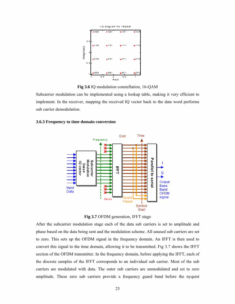
4.5 First stage of the decimation-in-frequency FFT algorithm. 37
4.6 Basic butterfly computation in the decimation-in-frequency 38
4.7 8-piont decimation-in-frequency FFT algorithm. 38
4.8 floating point representation 39
4.9 fixed point representation 40
5.1 simulation model of OFDM 43
5.2 BPSK constellation diagram 44
5.3 QPSK constellation diagram 45
5.4 16-QAM constellation diagram 45
5.5 64-QAM constellation diagram 46
5.6 BER vs. SNR plot for OFDM using BPSK, QPSK, 16-QAM, 64-QAM 48
5.7 BER vs. SNR of OFDM using BPSK modulation and fixed point FFT of word length 8
bits 50
5.8 BER vs. fraction length for OFDM using BPSK modulation and fixed point FFT of word
length 8 bits 50

vii
5.9 BER vs. SNR of OFDM using QPSK modulation and fixed point FFT of word length 8
bits 51
5.10 BER vs. fraction length for OFDM using QPSK modulation and fixed point FFT of
word length 8 bits 51
5.11 BER vs. SNR for OFDM using BPSK modulation and fixed point FFT of word length
16 bits 53
5.12 BER vs. fraction length of OFDM using BPSK modulation and fixed point FFT of word
length 16 bits 53
5.13 BER vs. for OFDM using QPSK modulation and fixed point FFT of word length 16 bits
54
5.14 BER vs. fraction length of OFDM using QPSK modulation and fixed point FFT of word
length 16 bits. 54
5.15. BER vs. SNR for OFDM using 16-QAM modulation and fixed point FFT of word
length 16 bits 55
5.16 BER vs. fraction length of OFDM using 16-QAM modulation and fixed point FFT of
word length 16 bits 55
5.17 BER vs. SNR for OFDM using 64-QAM modulation and fixed point FFT of word
length 16 bits 56
5.18 BER vs. fraction length of OFDM using 64-QAM modulation and fixed point FFT of
word length 16 bits. 56

viii
LIST OF TABLES
2.1 IEEE 802.11 standards 12 4.1 computations in DFT 32
4.2 computations in DFT & FFT 32
5.1 OFDM simulation parameters 47

ix
ABBREVIATIONS
AWGN additive White Gaussian Noise
ADSL asymmetric digital subscriber line
AP access point
BPSK binary phase shift keying
CCK complementary code keying
CSMA/CA Carrier Sense Multiple Access/ Collision Avoidance
CDMA code division multiple access
DSP digital signal processors
DAB digital audio broadcasting
DVB digital video broadcasting
DFT discrete Fourier transform
DSSS direct sequence spread spectrum
EP extension point
ETSI European Telecommunications Standards Institute
FCC Federal Communications Commission
FFT fast Fourier transform
FDM frequency division multiplexing
FEC forward error correction
HDTV high definition television
IEEE Institute of Electrical and Electronics Engineers
IFFT inverse Fourier transform
IDFT inverse discrete Fourier transform

x
ISI inter symbol interference
ICI inter carrier interference
LAN local area network
NTSC National Television Systems Committee
OFDM orthogonal frequency division multiplexing
PC personal computer
QPSK quadrature phase shift keying
QAM quadrature amplitude modulation
SNR signal to noise ratio
TDM time division multiplexing
TDMA time division multiple access
UHF ultra high frequency
VLSI very large scale integration
WLAN wireless local area networks

xi
NOMENCLATURE
CA (t) Amplitude of the carrier
c (t)ω Carrier frequency
c (t)φ Phase of the carrier
ss (t) Complex signal of OFDM
Fc Carrier frequency
FS Sampling rate
TS Length of the symbol in samples
TG Length of the guard period in samples
TFFT FFT period in samples
Lc Time of the channel in samples
Lp Cyclic prefix length in samples
x (n) original signal
X (k) Fourier transform of x (n)
knNW Twiddle factors
fΔ Subcarrier spacing
NFFT size of the FFT
f1 (n) even numbered samples
f2 (n) odd numbered samples
F1 (k) N/2-point DFT of f1 (n)
F2 (k) N/2-point DFT of f2 (n)

Chapter 1
INTRODUCTION

1.1 INTRODUCTION The ever increasing demand for very high rate wireless data transmission calls for
technologies which make use of the available electromagnetic resource in the most intelligent
way. Key objectives are spectrum efficiency (bits per second per Hertz), robustness against
multipath propagation, range, power consumption, and implementation complexity. These
objectives are often conflicting, so techniques and implementations are sought which offer
the best possible tradeoff between them.
The Internet revolution has created the need for wireless technologies that can deliver
data at high speeds in a spectrally efficient manner. However, supporting such high data rates
with sufficient robustness to radio channel impairments requires careful selection of
modulation techniques. Currently, the most suitable choice appears to be OFDM (Orthogonal
Frequency Division Multiplexing).The main reason that the OFDM technique has taken a
long time to become a prominence has been practical. It has been difficult to generate such a
signal, and even harder to receive and demodulate the signal. The hardware solution, which
makes use of multiple modulators and demodulators, was somewhat impractical for use in the
civil systems.
OFDM transmits a large number of narrowband carriers, closely spaced in the
frequency domain. In order to avoid a large number of modulators and filters at the
transmitter and complementary filters and demodulators at the receiver, it is desirable to be
able to use modern digital signal processing techniques, such as fast Fourier transform (FFT).
The ability to define the signal in the frequency domain, in software on VLSI (very
large scale integration) processors, and to generate the signal using the inverse Fourier
transform is the key to its current popularity. Although the original proposals were made a
long time ago, it has taken some time for technology to catch up.OFDM is currently being
used for digital audio and video broadcasting. OFDM for wireless LANs is being used every
where now, is operating in the unlicensed bands and is also being considered as a serious
candidate for fourth generation cellular systems.
This chapter begins with an exposition of the principle motivation behind the work
undertaken in this thesis. Following this section 1.3 provides literature survey on OFDM.
Section 1.4 discusses the contribution in this thesis. At the end, section 1.5 presents thesis
outline.

1.2 MOTIVATION OFDM is the modulation technique used in many new and emerging broadband
communication systems including wireless local area networks (WLANs), high definition
television (HDTV) and 4G systems. To achieve high data rates OFDM is used in wireless
LAN standards like IEEE 802.11a, IEEE 802.11g. The key component in an OFDM
transmitter is an inverse fast Fourier transform (IFFT) and in the receiver, an FFT. The
increasing computational power and performance capabilities of DSPs make them ideal for
the practical implementation of OFDM functions. Consumer products are usually sensitive to
cost and power consumption and for this reason, a fixed-point DSP approach is preferred.
However, fixed-point systems have limited dynamic range, causing the related problems of
round-off noise and arithmetic overflow.
The motivation for using OFDM techniques over TDMA techniques is twofold. First,
TDMA limits the total number of users that can be sent efficiently over a channel. In addition,
since the symbol rate of each channel is high, problems with multipath delay spread
invariably occur. In stark contrast, each carrier in an OFDM signal has a very narrow
bandwidth (i.e. 1 kHz); thus the resulting symbol rate is low. This results in the signal having
a high degree of tolerance to multipath delay spread, as the delay spread must be very long to
cause significant inter-symbol interference.
1.3 BACKGROUND LITERATURE SURVEY Orthogonal Frequency Division Multiplexing (OFDM) is an alternative wireless modulation
technology to CDMA. OFDM has the potential to surpass the capacity of CDMA systems
and provide the wireless access method for 4G systems. OFDM is a modulation scheme that
allows digital data to be efficiently and reliably transmitted over a radio channel, even in
multipath environments. In a typical orthogonal frequency division multiplexing (OFDM)
broadband wireless communication system, a guard interval using cyclic prefix is inserted to
avoid the intersymbol interference and the inter-carrier interference. This guard interval is
required to be at least equal to, or longer than the maximum channel delay spread. This
method is very simple, but it reduces the transmission efficiency. This efficiency is very low
in the communication systems, which inhibit a long channel delay spread with a small
number of sub-carriers such as the IEEE 802.11a wireless LAN (WLAN).
The origins of OFDM development started in the late 1950’s [1]. with the introduction
of Frequency Division Multiplexing (FDM) for data communications. In 1966 Chang

patented the structure of OFDM [2] and published [3] the concept of using orthogonal
overlapping multi-tone signals for data communications. In 1971 Weinstein [4] introduced
the idea of using a Discrete Fourier Transform (DFT) for implementation of the generation
and reception of OFDM signals, eliminating the requirement for banks of analog subcarrier
oscillators. This presented an opportunity for an easy implementation of OFDM, especially
with the use of Fast Fourier Transforms (FFT), which are an efficient implementation of the
DFT. This suggested that the easiest implementation of OFDM is with the use of Digital
Signal Processing (DSP), which can implement FFT algorithms. It is only recently that the
advances in integrated circuit technology have made the implementation of OFDM cost
effective. The reliance on DSP prevented the wide spread use of OFDM during the early
development of OFDM. It wasn’t until the late 1980’s that work began on the development of
OFDM for commercial use, with the introduction of the Digital Audio Broadcasting (DAB)
system.
1.3.1 Digital audio broadcasting
DAB was the first commercial use of OFDM technology [5]. Development of DAB started in
1987 and services began in U.K and Sweden in1995. DAB is a replacement for FM audio
broadcasting, by providing high quality digital audio and information services. OFDM was
used for DAB due to its multipath tolerance.
Broadcast systems operate with potentially very long transmission distances (20 -100
km). As a result, multipath is a major problem as it causes extensive ghosting of the
transmission. This ghosting causes Inter-Symbol Interference (ISI), blurring the time domain
signal.
For single carrier transmissions the effects of ISI are normally mitigated using
adaptive equalization. This process uses adaptive filtering to approximate the impulse
response of the radio channel. An inverse channel response filter is then used to recombine
the blurred copies of the symbol bits. This process is however complex and slow due to the
locking time of the adaptive equalizer. Additionally it becomes increasing difficult to
equalize signals that suffer ISI of more than a couple of symbol periods.
OFDM overcomes the effects of multipath by breaking the signal into many narrow
bandwidth carriers. This results in a low symbol rate reducing the amount of ISI. In addition
to this, a guard period is added to the start of each symbol, removing the effects of ISI for
multipath signals delayed less than the guard period. The high tolerance to multipath makes
OFDM more suited to high data transmissions in terrestrial environments than single carrier
transmissions.

The data throughput of DAB varies from 0.6 - 1.8 Mbps depending on the amount of
Forward Error Correction (FEC) applied. This data payload allows multiple channels to be
broadcast as part of the one transmission ensemble. The number of audio channels is variable
depending on the quality of the audio and the amount of FEC used to protect the signal. For
telephone quality audio (24 kbps) up to 64 audio channels can be provided, while for CD
quality audio (256 kb/s), with maximum protection, three channels are available.
1.3.2 Digital video broadcasting
The development of the Digital Video Broadcasting (DVB) standards was started in 1993.
DVB is a transmission scheme based on the MPEG-2 standard, as a method for point to
multipoint delivery of high quality compressed digital audio and video. It is an enhanced
replacement of the analogue television broadcast standard, as DVB provides a flexible
transmission medium for delivery of video, audio and data services [6]. The DVB standards
specify the delivery mechanism for a wide range of applications, including satellite TV
(DVB-S), cable systems (DVB-C) and terrestrial transmissions (DVB-T). The physical layer
of each of these standards is optimized for the transmission channel being used. Satellite
broadcasts use a single carrier transmission, with QPSK modulation, which is optimized for
this application as a single carrier allows for large Doppler shifts, and QPSK allows for
maximum energy efficiency [7]. This transmission method is however unsuitable for
terrestrial transmissions as multipath severely degrades the performance of high-speed single
carrier transmissions. For this reason, OFDM was used for the terrestrial transmission
standard for DVB. The physical layer of the DVB-T transmission is similar to DAB, in that
the OFDM transmission uses a large number of subcarriers to mitigate the effects of
multipath. DVB-T allows for two transmission modes depending on the number of
subcarriers used [8].The major difference between DAB and DVB-T is the larger bandwidth
used and the use of higher modulation schemes to achieve a higher data throughput. The
DVB-T allows for three subcarrier modulation schemes: QPSK, 16-QAM (Quadrature
Amplitude Modulation) and 64- QAM; and a range of guard period lengths and coding rates.
This allows the robustness of the transmission link to be traded at the expense of link capacity.
1.3.3 Hiperlan2 and IEEE802.11a
Development of the European Hiperlan standard was started in 1995, with the final standard
of HiperLAN2 being defined in June 1999. HiperLAN2 pushes the performance of WLAN
systems, allowing a data rate of up to 54 Mbps [9]. HiperLAN2 uses 48 data and 4 pilot
subcarriers in a 16 MHz channel, with 2 MHz on either side of the signal to allow out of band

roll off. User allocation is achieved by using TDM, and subcarriers are allocated using a
range of modulation schemes, from BPSK up to 64-QAM, depending on the link quality.
Forward Error Correction is used to compensate for frequency selective fading. IEEE802.11a
has the same physical layer as HiperLAN2 with the main difference between the standard
corresponding to the higher-level network protocols used.HiperLAN2 is used extensively as
an example OFDM system in this thesis. Since the physical layer of HiperLAN2 is very
similar to the IEEE802.11a standard these examples are applicable to both standards.
The most important advantage of the OFDM transmission technique as compared to
single carrier systems is obtained in frequency-selective channels. The signal processing in
the receiver is rather simple in this case, because after transmission over the radio channel the
orthogonality of the OFDM subcarriers is maintained and the channel interference effect is
reduced to a multiplication of each subcarrier by a complex transfer factor. Therefore,
equalizing the signal is very simple, whereas equalization may not be feasible in the case of
conventional single carrier transmission covering the same bandwidth. It must be mentioned,
however, that in [10] a single carrier system with frequency domain equalization has been
proposed which also copes with large delays.
1.4 THESIS CONTRIBUTION The huge uptake rate of Wireless Local Area Networks (WLAN) and the exponential growth
of the Internet have resulted in an increased demand for new methods of obtaining high
capacity wireless networks. WLAN standards such as IEEE802.11a, IEEE 802.11g are based
on OFDM technology and provide a much higher data rate of 54 Mbps. However systems of
the near future will require WLANs with data rates of greater than 100 Mbps, and so there is
a need to further improve the spectral efficiency and data capacity of OFDM systems in
WLAN applications.
So the OFDM system was simulated using different modulation schemes like BPSK,
QPSK, 16-QAM, and 64-QAM to achieve different data rates according to IEEE 802.11a
wireless LAN standard specifications. Its immunity to multipath delay spread was tested for
BPSK modulation by considering different cyclic prefix lengths. In the OFDM simulation
floating point FFT was used. Generally Floating point processors are more expensive because
they implement more functionality (complexity) and consume more power. The effects of
fixed point FFT on OFDM system were simulated for different combinations of integer part
lengths and fraction lengths.

1.5 THESIS OUTLINE Following this introduction chapter, Chapter 2 discusses definition of wireless LAN, wireless
LAN technologies, and wireless LAN standards (IEEE 802.11, IEEE 802.11a, and IEEE
802.11b, IEEE 802.11g) in detail.
Chapter 3 provides an introduction to OFDM in general and outlines some of the
problems associated with it. This chapter describes what OFDM is, and how it can be
generated and received. It also looks at why OFDM is a robust modulation scheme and some
of its advantages and disadvantages over single carrier modulation schemes. It also discusses
the some of the applications of OFDM.
Chapter 4 discusses about decimation in time and decimation in frequency radix-2 fast
Fourier transform algorithms. It also presents the representation of floating point and fixed
point numbers. It also discusses about the dynamic range of a fixed point variable based on
their word lengths and fraction lengths and finite word length effects.
Chapter 5 provides the results obtained in this thesis, and their discussions. It provides
the OFDM system model used in the simulation. It discusses about the modulation schemes
used in the simulation and their constellation diagrams. It shows the results of bit error rate
performance against signal to noise ratio for different modulation schemes used in wireless
LAN standards .it also discusses about the simulation results of OFDM using fixed point FFT
for input word lengths of 8 bits and 16 bits and compares these results with OFDM using
floating point FFT.
Chapter 6 discusses about the achievement of the thesis work, limitations of the work,
and future directions of the work.

Chapter 2
WLAN TECHNOLOGIES & STANDARDS

7
2.1INTRODUCTION “A Wireless Local Area Network is a data communications system which transmits and
receives data over the air using radio technology.” as the name suggests it makes use of
wireless transmission medium. In earlier days they were not so popular. The reasons for these
included high prices, low data rates and licensing requirements. As these problems have been
addressed, the popularity of wireless LANs has grown rapidly.
Wireless LANs redefine the way we view LANs.connecivity no longer implies physical
attachment. Users can remain connected to the network as they move around the building or
campus. There is no need anymore to bury the network infrastructure in the ground or hide it
behind the walls. With wireless networking, the network infrastructure can move and change
at the speed of the organization.
Wireless LANs are used both in business and home environments, either as
extensions to existing networks, or, in smaller environments, as alternatives to wired
networks. They provide all the benefits and features of traditional LANs. Over the last seven
years, WLANs have gained strong popularity in a number of vertical markets, including the
health-care, retail, manufacturing, warehousing, and academic arenas. These industries have
profited from the productivity gains of using hand-held terminals and notebook computers to
transmit real-time information to centralized hosts for processing. Today WLANs are
becoming more widely recognized as a general-purpose connectivity alternative for a broad
range of business customers.
This chapter is organized as follows. Following this introduction, section 2.2
discusses the need for wireless LAN, its advantages over wired LAN. Section 2.3 discusses
the different wireless LAN technologies. Section 2.4 discusses the various WLAN standards
(IEEE 802.11, IEEE802.11a, IEEE 802.11b, IEEE 802.11g) etc. finally section 2.5 concludes
the chapter.
2.2 WHY WIRELESS? The widespread reliance on networking in business and the meteoric growth of the Internet and
online services are strong testimonies to the benefits of shared data and shared resources [11].
With wireless LANs, users can access shared information without looking for a place to plug in,
and network managers can set up or augment networks without installing or moving wires.
Wireless LANs offer the following productivity, convenience, and cost advantages over
traditional wired networks:

8
Mobility: Wireless LAN systems can provide LAN users with access to real-time
information anywhere in their organization. This mobility supports productivity and
service opportunities not possible with wired networks.
Installation Speed and Simplicity: Installing a wireless LAN system can be fast and
easy and can eliminate the need to pull cable through walls and ceilings.
Installation Flexibility: Wireless technology allows the network to go where wire cannot
go.
Reduced Cost-of-Ownership: While the initial investment required for wireless LAN
hardware can be higher than the cost of wired LAN hardware, overall installation
expenses and life-cycle costs can be significantly lower. Long-term cost benefits are
greatest in dynamic environments requiring frequent moves and changes.
Scalability: Wireless LAN systems can be configured in a variety of topologies to meet
the needs of specific applications and installations. Configurations are easily changed and
range from peer-to-peer networks suitable for a small number of users to full
infrastructure networks of thousands of users that enable roaming over a broad area.
2.3 WIRELESS LAN TECHNOLOGIES The technologies available for use in WLANs include infrared, UHF (narrowband) radios, and
spread spectrum radios. Two spread spectrum techniques are currently prevalent: frequency
hopping and direct sequence. In the United States, the radio bandwidth used for spread
spectrum communications falls in three bands (900 MHz, 2.4 GHz, and 5.7 GHz), which the
Federal Communications Commission (FCC) approved for local area commercial
communications in the late 1980s. In Europe, ETSI, the European Telecommunications
Standards Institute, introduced regulations for 2.4 GHz in 1994, and Hiperlan is a family of
standards in the 5.15-5.7 GHz and 19.3 GHz frequency bands [12].
2.3.1 Infrared (IR) Infrared is an invisible band of radiation that exists at the lower end of the visible
electromagnetic spectrum. This type of transmission is most effective when a clear line-of-sight
exists between the transmitter and the receiver. Two types of infrared WLAN solutions are
available: diffused-beam and direct-beam (or line-of-sight). Currently, direct-beam WLANs
offer a faster data rate than diffused-beam networks, but is more directional since diffused-
beam technology uses reflected rays to transmit/receive a data signal, it achieves lower data
rates in the 1-2 Mbps range.

9
Infrared optical signals are often used in remote control device applications. Users who
can benefit from infrared include professionals who continuously set up temporary offices,
such as auditors, salespeople, consultants, and managers who visit customers or branch offices.
These users connect to the local wired network via an infrared device for retrieving information
or using fax and print functions on a server.
A group of users may also set up a peer-to peer infrared network while on location to
share printer, fax, or other server facilities within their own LAN environment. The education
and medical industries commonly use this configuration to easily move networks. Infrared is a
short range technology. When used indoors, it can be limited by solid objects such as doors,
walls, merchandise, or racking. In addition, the lighting environment can affect signal quality.
For example, loss of communications may occur because of the large amount of sunlight or
background light in an environment. Fluorescent lights also may contain large amounts of
infrared. This problem may be solved by using high signal power and an optical bandwidth
filter, which lessens the infrared signals coming from outside sources. In an outdoor
environment, snow, ice, and fog may affect the operation of an infrared based system. Because
of its many limitations, infrared is not a very popular technology for WLANs.
Advantages:
No government regulation controlling use.
Immunity To electro magnetic (EM) and RF interference.
Disadvantages:
Generally a short range technology(30-50 ft under ideal conditions)
Signals cannot penetrate solid objects.
Signal affected by light, snow, ice, fog.
Dirt can interfere with infrared.
2.3.2 Narrowband technology
A narrowband radio system transmits and receives user information on a specific radio
frequency. Narrowband radio keeps the radio signal frequency as narrow as possible just to
pass the information. Undesirable crosstalk between communications channels is avoided by
carefully coordinating different users on different channel frequencies.
A private telephone line is much like a radio frequency. When each home in a
neighborhood has its own private telephone line, people in one home cannot listen to calls
made to other homes. In a radio system, privacy and noninterference are accomplished by the
use of separate radio frequencies. The radio receiver filters out all radio signals except the ones
on its designated frequency.

10
Advantages:
Longest range.
Low cost solution for large sites with low to medium data throughput requirements.
Disadvantages:
Large radio and antennas increase wireless client size.
RF site license required for protected bands.
No multivendor interoperability.
Low throughput and interference potential.
2.3.3 Spread Spectrum Technology
Most wireless LAN systems use spread-spectrum technology, a wideband radio frequency
technique developed by the military for use in reliable, secure, mission-critical communications
systems. Spread-spectrum is designed to trade off bandwidth efficiency for reliability, integrity,
and security. In other words, more bandwidth is consumed than in the case of narrowband
transmission, but the tradeoff produces a signal that is, in effect, louder and thus easier to detect,
provided that the receiver knows the parameters of the spread-spectrum signal being broadcast.
If a receiver is not tuned to the right frequency, a spread-spectrum signal looks like background
noise. There are two types of spread spectrum radio: frequency hopping and direct sequence.
Frequency-Hopping Spread Spectrum Technology
Frequency-hopping spread-spectrum (FHSS) uses a narrowband carrier that changes frequency
in a pattern known to both transmitter and receiver. Properly synchronized, the net effect is to
maintain a single logical channel. To an unintended receiver, FHSS appears to be short
duration impulse noise.
Direct-Sequence Spread Spectrum Technology
Direct-sequence spread-spectrum (DSSS) generates a redundant bit pattern for each bit to be
transmitted. This bit pattern is called a chip (or chipping code). The longer the chip, the greater
the probability that the original data can be recovered (and, of course, the more bandwidth
required). Even if one or more bits in the chip are damaged during transmission, statistical
techniques embedded in the radio can recover the original data without the need for
retransmission. To an unintended receiver, DSSS appears as low-power wideband noise and is
rejected (ignored) by most narrowband receivers.

11
2.3.4 Orthogonal frequency division multiplexing
Orthogonal frequency division multiplexing, also called multi carrier modulation uses multiple
carrier signals at different frequencies, sending some of bits on each channel. This is similar to
FDM.How ever, in the case of OFDM, all sub channels are dedicated to a single data source.
In the OFDM, Suppose we have a data stream operating at R bps and an available
bandwidth of NΔf, centerd at f0.theentire bandwidth could be used to send data stream, in
which case each bit duration would be 1/R.The alternative is to split the data stream into N
substreams, using a serial to parallel converter. Each substream has a data rate of R/Nbps and is
transmitted on a separate subcarrier, with spacing between adjacent subcarriers of Δf.now the
bit duration is N/R.
OFDM has several advantages. First, frequency selective fading only affects some sub
channels and not the whole signal. If the data stream is protected by a forward error correcting
code, this type of fading is easily handled. More important, OFDM overcome inter symbol
interference (ISI) in a multipath environment’s has greater impact at higher bit rates, because
the distance between bits or symbols is smaller. With OFDM, the data rate is reduced by a
factor of N, which increases the symbol time by a factor of N. thus if the symbol period is Ts
for the source stream, the period for the OFDM signals is NTs. This dramatically reduces the
effect of ISI.as a design criterion, N is chosen so that NTs is significantly greater than the root
mean square delay spread of the channel.
2.4 STANDARDS Nowhere in the modern computing field is the proliferation of acronyms and numerical
designators more prevalent than in wireless networking. Here is the short version of what you
need to know to bring some order to the chaos. 2.4.1 802. What?
The IEEE (Institute of Electrical and Electronics Engineers) is the body responsible for
setting standards for computing devices. They have established a committee to set standards
for Local Area and Metropolitan Area Networking named the “802 LMSC” (LAN MAN
Standards Committee). Within this committee there are workgroups tasked with specific
responsibilities, and given a numeric designation such as “11”. In this case the 802.11
workgroup is tasked with developing the standards for wireless networking [13].
Within this 802.11 workgroup, there are task groups with even more specific tasks,
and these groups are designated with an alphabetic character such as “a”, or “b”, or “g”.

12
There is no apparent logic to the ordering of these characters and none should be inferred.
The specific groups and tasks concerning wireless networking hardware standards are
outlined below.
Table 2.1 IEEE 802.11 standards
2.4.2 IEEE 802.11
The original version of the standard IEEE 802.11 released in 1997 specifies two raw data
rates of 1 and 2 megabits per second (Mbit/s) to be transmitted via infrared (IR) signals or by
either Frequency hopping or Direct-sequence spread spectrum in the Industrial Scientific
Medical frequency band at 2.4 GHz. IR remains a part of the standard but has no actual
implementations. The original standard also defines Carrier Sense Multiple Access with
Collision Avoidance (CSMA/CA) as the medium access method. A significant percentage of
the available raw channel capacity is sacrificed (via the CSMA/CA mechanisms) in order to
improve the reliability of data transmissions under diverse and adverse environmental
conditions.
2.4.3 IEEE 802.11a
The 802.11a amendment to the original standard was ratified in 1999. The 802.11a standard
uses the same core protocol as the original standard, operates in 5 GHz band, and uses a 52-
subcarrier orthogonal frequency-division multiplexing (OFDM) with a maximum raw data
rate of 54 Mb/s, which yields realistic net achievable throughput in the mid-20 Mb/s. The
data rate is reduced to 48, 36, 24, 18, 12, 9 then 6 Mb/s if required.
802.11a is not interoperable with 802.11b as they operate on separate bands, except if
using equipment that has a dual band capability. Nearly all enterprise class Access Points has
dual band capability. Since the 2.4 GHz band is heavily used, using the 5 GHz band gives
Standard Release date Op.frequency band Max.data rate
IEEE 802.11 1997 2.4GHz 2Mbps
IEEE 802.11a 1999 5GHz 54Mbps
IEEE 802.11b 1999 2.4GHz 11Mbps
IEEE 802.11g 2003 2.4GHz 54Mbps
IEEE 802.11n 2007(projected) 2.4GHz or 5GHz 540Mbps

13
802.11a a significant advantage. However, this high carrier frequency also brings a slight
disadvantage. The effective overall range of 802.11a is slightly less then 802.11b/g, it also
means that 802.11a cannot penetrate as far as 802.11b since it is absorbed more readily when
penetrating multiple walls. On the other hand, OFDM has fundamental propagation
advantages when in a high multipath environment such as an indoor office. And the higher
frequencies enable the building of smaller antennae with higher RF system gain which
counteract the disadvantage of a higher band of operation. The increased number of useable
channels (4 to 8 times as many in FCC countries) and the near absence of other interfering
systems (microwave ovens, cordless phones, bluetooth products) makes the 5 GHz band the
preferred band for professionals and businesses who require more capacity and reliability and
are willing to pay a small premium for it.
2.4.4 IEEE 802.11b
The 802.11b amendment to the original standard was ratified in 1999. 802.11b has a
maximum raw data rate of 11 Mb/s and uses the same CSMA/CA media access method
defined in the original standard.802.11b products appeared on the market in early 2000, since
802.11b is a direct extension of the DSSS (Direct-sequence spread spectrum) modulation
technique defined in the original standard. Technically, the 802.11b standard uses
Complementary code keying (CCK) as its modulation technique. The dramatic increase in
throughput of 802.11b (compared to the original standard) along with simultaneous
substantial price reductions led to the rapid acceptance of 802.11b as the definitive wireless
LAN technology.
2.4.5 IEEE 802.11g
In June 2003, a third modulation standard was ratified: 802.11g.This flavor works in the 2.4
GHz band (like 802.11b) but operates at a maximum raw data rate of 54 Mb/s, or about 19
Mb/s net throughput (like 802.11a except with some additional legacy overhead). 802.11g
hardware is backwards compatible with 802.11b hardware. Details of making b and g work
well together occupied much of the lingering technical process. In an 11g network, however,
the presence of an 802.11b participant does significantly reduce the speed of the overall
802.11g network.
The modulation scheme used in 802.11g is orthogonal frequency-division
multiplexing (OFDM) for the data rates of 6, 9, 12, 18, 24, 36, 48, and 54 Mb/s, and reverts
to CCK (like the 802.11b standard) for 5.5 and 11 Mb/s and DBPSK/DQPSK+DSSS for 1
and 2 Mb/s. Even though 802.11g operates in the same frequency band as 802.11b, it can

14
achieve higher data rates because of its similarities to 802.11a. The maximum range of
802.11g devices is slightly greater than that of 802.11b devices, but the range in which a
client can achieve the full 54 Mb/s data rate is much shorter than that of which a 802.11b
client can reach 11 Mb/s.
2.5 CONCLUSION In this chapter, detailed description of different wireless LAN technologies was presented. It
also discussed about different wireless LAN standards like IEEE 802.11, IEEE 802.11a,
IEEE 802.11b, IEEE 802.11g etc. and the modulation techniques they use.

Chapter 3
OFDM

15
3.1 INTRODUCTION The principle of orthogonal frequency division multiplexing (OFDM) modulation has been in
existence for several decades. However, in recent years these techniques have quickly moved
out of textbooks and research laboratories and into practice in modern communications
systems. The techniques are employed in data delivery systems over the phone line, digital
radio and television, and wireless networking systems [14]. What is OFDM? And why has it
recently become so popular?
This chapter is organized as follows. Following this introduction, section 3.2, 3.3
gives brief details about single carrier modulation, FDM modulation systems. Section 3.4
discusses definition of orthogonality, and principle of OFDM.section 3.5 discusses the how
FFT maintains orthogonality.section 3.6 discusses the generation and reception of OFDM in
detail. Section 3.7 addresses about the guard period used in OFDM systems. Section 3.8
presents the advantages, disadvantages and applications of OFDM. finally section 3.9
concludes the chapter.
3.2 THE SINGLE CARRIER MODULATION SYSTEM
Fig.3.1 Single carrier spectrum
A typical single-carrier modulation spectrum is shown in Figure 3.1. A single carrier system
modulates information onto one carrier using frequency, phase, or amplitude adjustment of
the carrier. For digital signals, the information is in the form of bits, or collections of bits
called symbols, that are modulated onto the carrier. As higher bandwidths (data rates) are
used, the duration of one bit or symbol of information becomes smaller. The system becomes
more susceptible to loss of information from impulse noise, signal reflections and other
impairments. These impairments can impede the ability to recover the information sent. In
addition, as the bandwidth used by a single carrier system increases, the susceptibility to

16
interference from other continuous signal sources becomes greater. This type of interference
is commonly labeled as carrier wave (CW) or frequency interference.
3.3 FREQUENCY DIVISION MULTIPLEXING MODULATION SYSTEM A typical Frequency division multiplexing signal spectrum is shown in figure 3.2.FDM
extends the concept of single carrier modulation by using multiple sub carriers within the
same single channel. The total data rate to be sent in the channel is divided between the
various sub carriers. The data do not have to be divided evenly nor do they have to originate
from the same information source. Advantages include using separate modulation
demodulation customized to a particular type of data, or sending out banks of dissimilar data
that can be best sent using multiple, and possibly different, modulation schemes.
Fig 3.2 FDM signal spectrum
Current national television systems committee (NTSC) television and FM stereo multiplex
are good examples of FDM. FDM offers an advantage over single-carrier modulation in
terms of narrowband frequency interference since this interference will only affect one of the
frequency sub bands. The other sub carriers will not be affected by the interference. Since
each sub carrier has a lower information rate, the data symbol periods in a digital system will
be longer, adding some additional immunity to impulse noise and reflections. FDM systems
usually require a guard band between modulated sub carriers to prevent the spectrum of one
sub carrier from interfering with another. These guard bands lower the system’s effective
information rate when compared to a single carrier system with similar modulation.
3.4 ORTHOGONALITY AND OFDM If the FDM system above had been able to use a set of sub carriers that were orthogonal to
each other, a higher level of spectral efficiency could have been achieved. The guard bands
that were necessary to allow individual demodulation of sub carriers in an FDM system
would no longer be necessary. The use of orthogonal sub carriers would allow the sub

17
carriers’ spectra to overlap, thus increasing the spectral efficiency. As long as orthogonality is
maintained, it is still possible to recover the individual sub carriers’ signals despite their
overlapping spectrums. If the dot product of two deterministic signals is equal to zero, these
signals are said to be orthogonal to each other. Orthogonality can also be viewed from the
standpoint of stochastic processes. If two random processes are uncorrelated, then they are
orthogonal. Given the random nature of signals in a communications system, this
probabilistic view of orthogonality provides an intuitive understanding of the implications of
orthogonality in OFDM.
OFDM is implemented in practice using the discrete Fourier transform (DFT). Recall
from signals and systems theory that the sinusoids of the DFT form an orthogonal basis set,
and a signal in the vector space of the DFT can be represented as a linear combination of the
orthogonal sinusoids. One view of the DFT is that the transform essentially correlates its
input signal with each of the sinusoidal basis functions. If the input signal has some energy at
a certain frequency, there will be a peak in the correlation of the input signal and the basis
sinusoid that is at that corresponding frequency. This transform is used at the OFDM
transmitter to map an input signal onto a set of orthogonal sub carriers, i.e., the orthogonal
basis functions of the DFT. Similarly, the transform is used again at the OFDM receiver to
process the received sub carriers. The signals from the sub carriers are then combined to form
an estimate of the source signal from the transmitter. The orthogonal and uncorrelated nature
of the sub carriers is exploited in OFDM with powerful results. Since the basis functions of
the DFT are uncorrelated, the correlation performed in the DFT for a given sub carrier only
sees energy for that corresponding sub carrier. The energy from other sub carriers does not
contribute because it is uncorrelated. This separation of signal energy is the reason that the
OFDM sub carriers’ spectrums can overlap without causing interference.
3.5 MATHEMATICAL ANALYSIS: With an overview of the OFDM system, it is valuable to discuss the mathematical definition
of the modulation system. It is important to understand that the carriers generated by the IFFT
chip are mutually orthogonal. This is true from the very basic definition of an IFFT signal.
This will allow understanding how the signal is generated and how receiver must operate.
Mathematically, each carrier can be described as a complex wave:
cj( ( t ) c(t ))C CS (t) A (t)e ω +Φ= (3.1)

18
The real signal is the real part of sc (t). Ac (t) and φc (t), the amplitude and phase of the
carrier, can vary on a symbol by symbol basis. The values of the parameters are constant over
the symbol duration period t. OFDM consists of many carriers. Thus the complex signal Ss(t)
is represented by:
n n
N 1j[ t ( t )]
s Nn 0
1s (t) A (t)eN
−ω +φ
=
= ∑ (3.2)
Where
n o nω = ω + Δω
This is of course a continuous signal. If we consider the waveforms of each component of the
signal over one symbol period, then the variables Ac (t) and φc (t) take on fixed values,
which depend on the frequency of that particular carrier, and so can be rewritten:
n n
n n
(t)A (t) Aφ = φ
=
If the signal is sampled using a sampling frequency of 1/T, then the resulting signal is
represented by:
0 n
N 1[ j( n )kT ]
s nn 0
1s (kT) A eN
−ω + Δω +φ
=
= ∑ (3.3)
At this point, we have restricted the time over which we analyze the signal to N samples. It is
convenient to sample over the period of one data symbol. Thus we have a relationship: t=NT
If we now simplify equation 3.3, without a loss of generality by letting ω0=0, then the signal
becomes:
n
N 1j j(n )kT
s nN 0
1s (kT) A e eN
−φ Δω
=
= ∑ (3.4)
Now equation 3.4 can be compared with the general form of the inverse Fourier transform: 2N 1 knN
n 0
1 ng(kT) G ( )eN NT
π−
=
= ∑ (3.5)
In Equation 3.4 the function nj
nA e φis no more than a definition of the signal in the
sampled frequency domain, and s (kT) is the time domain representation. Eqns.4 and 5 are
equivalent if:

19
This is the same condition that was required for orthogonality Thus, one consequence of
maintaining orthogonality is that the OFDM signal can be defined by using Fourier transform
procedures.
3.6 OFDM GENERATION AND RECEPTION OFDM signals are typically generated digitally due to the difficulty in creating large banks of
phase locks oscillators and receivers in the analog domain. Fig 3.3 shows the block diagram
of a typical OFDM transceiver [15]. The transmitter section converts digital data to be
transmitted, into a mapping of subcarrier amplitude and phase. It then transforms this spectral
representation of the data into the time domain using an Inverse Discrete Fourier Transform
(IDFT). The Inverse Fast Fourier Transform (IFFT) performs the same operations as an IDFT,
except that it is much more computationally efficiency, and so is used in all practical systems.
In order to transmit the OFDM signal the calculated time domain signal is then mixed up to
the required frequency.
Fig 3.3 Block diagram of a basic OFDM transceiver.
The receiver performs the reverse operation of the transmitter, mixing the RF signal to base
band for processing, then using a Fast Fourier Transform (FFT) to analyze the signal in the
frequency domain [16]. The amplitude and phase of the sub carriers is then picked out and
converted back to digital data. The IFFT and the FFT are complementary function and the
most appropriate term depends on whether the signal is being received or generated. In cases
cj.2.π.f .te Serial to parallel converter
Modulation And Mapping
IFFT
Cyclic prefix insertion
Parallel to serial converter
Channel
Serial to parallel converter
FFT
Cyclic prefix extraction
Demapping And
Demodulation
Parallel to serial
cj.2.π.f .te
data
Recovered data

20
where the signal is independent of this distinction then the term FFT and IFFT is used
interchangeably.
3.6.1 Serial to parallel conversion
Data to be transmitted is typically in the form of a serial data stream. In OFDM, each symbol
typically transmits 40 - 4000 bits, and so a serial to parallel conversion stage is needed to
convert the input serial bit stream to the data to be transmitted in each OFDM symbol. The
data allocated to each symbol depends on the modulation Scheme used and the number of sub
carriers. For example, for a sub carrier modulation of 16 QAM each sub carrier carries 4 bits
of data, and so for a transmission using 100 sub carriers the number of bits per symbol would
be 400.
At the receiver the reverse process takes place, with the data from the sub carriers
being converted back to the original serial data stream. When an OFDM transmission occurs
in a multipath radio environment, frequency selective fading can result in groups of sub
carriers being heavily attenuated, which in turn can result in bit errors. These nulls in the
frequency response of the channel can cause the information sent in neighbouring carriers to
be destroyed, resulting in a clustering of the bit errors in each symbol. Most Forward Error
Correction (FEC) schemes tend to work more effectively if the errors are spread evenly,
rather than in large clusters, and so to improve the performance most systems employ data
scrambling as part of the serial to parallel conversion stage. This is implemented by
randomizing the sub carrier allocation of each sequential data bit. At the receiver the reverse
scrambling is used to decode the signal. This restores the original sequencing of the data bits,
but spreads clusters of bit errors so that they are approximately uniformly distributed in time.
This randomization of the location of the bit errors improves the performance of the FEC and
the system as a whole.
3.6.2 Subcarrier modulation
Modulation: An Introduction
One way to communicate a message signal whose frequency spectrum does not fall within
that fixed frequency range, or one that is otherwise unsuitable for the channel, is to change a
transmittable signal according to the information in the message signal. This alteration is
called modulation, and it is the modulated signal that is transmitted. The receiver then
recovers the original signal through a process called demodulation.
Modulation is a process by which a carrier signal is altered according to information
in a message signal. The carrier frequency, denoted Fc, is the frequency of the carrier signal.

21
The sampling rate, Fs, is the rate at which the message signal is sampled during the
simulation. The frequency of the carrier signal is usually much greater than the highest
frequency of the input message signal. The Nyquist sampling theorem requires that the
simulation sampling rate Fs be greater than two times the sum of the carrier frequency and
the highest frequency of the modulated signal, in order for the demodulator to recover the
message correctly.
Baseband versus Pass band Simulation
For a given modulation technique, two ways to simulate modulation techniques are called
baseband and pass band. Baseband simulation requires less computation. In this thesis,
baseband simulation will be used.
Digital Modulation Techniques
a) Amplitude Shift Key (ASK) Modulation
Fig 3.4 ASK modulation
In this method the amplitude of the carrier assumes one of the two amplitudes dependent on
the logic states of the input bit stream. A typical output waveform of an ASK modulation is
shown in Fig3.4.
b) Frequency Shift Key (FSK) Modulation
In this method the frequency of the carrier is changed to two different frequencies depending
on the logic state of the input bit stream. The typical output waveform of an FSK is shown in
Fig 3.5. Notice that logic high causes the centre frequency to increase to a maximum and a
logic low causes the centre frequency to decrease to a minimum.

22
Fig. 3.5 FSK Modulation
c) Phase Shift Key (PSK) Modulation
With this method the phase of the carrier changes between different phases determined by the
logic states of the input bit stream. There are several different types of Phase Shift Key (PSK)
modulators. These are:
Two-phase (2 PSK)
Four-phase (4 PSK)
Eight-phase (8 PSK)
Sixteen-phase (16 PSK) etc.
d) Quadrature Amplitude Modulation (QAM)
QAM is a method for sending two separate (and uniquely different) channels of information.
The carrier is shifted to create two carriers namely the sine and cosine versions. The outputs
of both modulators are algebraically summed and the result of which is a single signal to be
transmitted, containing the In-phase (I) and Quadrature (Q) information. The set of possible
combinations of amplitudes is a pattern of dots known as a QAM constellation.
Once each subcarrier has been allocated bits for transmission, they are mapped using
a modulation scheme to a subcarrier amplitude and phase, which is represented by a complex
In-phase and Quadrature-phase (IQ) vector. Fig 3.6 shows an example of subcarrier
modulation mapping. This example shows 16-QAM, which maps 4 bits for each symbol.
Each combination of the 4 bits of data corresponds to a unique IQvector, shown as a dot on
the figure. A large number of modulation schemes are available allowing the number of bits
transmitted per carrier per symbol to be varied [17].
23
Fig 3.6 IQ modulation constellation, 16-QAM
Subcarrier modulation can be implemented using a lookup table, making it very efficient to
implement. In the receiver, mapping the received IQ vector back to the data word performs
sub carrier demodulation.
3.6.3 Frequency to time domain conversion
Fig 3.7 OFDM generation, IFFT stage
After the subcarrier modulation stage each of the data sub carriers is set to amplitude and
phase based on the data being sent and the modulation scheme. All unused sub carriers are set
to zero. This sets up the OFDM signal in the frequency domain. An IFFT is then used to
convert this signal to the time domain, allowing it to be transmitted. Fig 3.7 shows the IFFT
section of the OFDM transmitter. In the frequency domain, before applying the IFFT, each of
the discrete samples of the IFFT corresponds to an individual sub carrier. Most of the sub
carriers are modulated with data. The outer sub carriers are unmodulated and set to zero
amplitude. These zero sub carriers provide a frequency guard band before the nyquist

24
frequency and effectively act as an interpolation of the signal and allows for a realistic roll off
in the analog anti-aliasing reconstruction filters.
3.6.4 RF modulation
The output of the OFDM modulator generates a base band signal, which must be mixed up to
the required transmission frequency. This can be implemented using analog techniques as
shown in Fig 3.8 or using a Digital up Converter as shown in Fig 3.9.
Fig 3.8 RF modulation of complex base band OFDM signal, using analog techniques
Fig.3.9 RF modulation of complex base band OFDM signal, using digital techniques.

25
Both techniques perform the same operation, however The performance of the digital
modulation will tend to be more accurate due to improved matching between the processing
of the I and Q channels, and the phase accuracy of the digital IQ modulator.
3.7 GUARD PERIOD For a given system bandwidth the symbol rate for an OFDM signal is much lower than a
single carrier transmission scheme. For example for a single carrier BPSK modulation, the
symbol rate corresponds to the bit rate of the transmission. However for OFDM the system
bandwidth is broken up into NC sub carriers, resulting in a symbol rate that is NC times lower
than the single carrier transmission. This low symbol rate makes OFDM naturally resistant to
effects of Inter-Symbol Interference (ISI) caused by multipath propagation. Multipath
propagation is caused by the radio transmission signal reflecting off objects in the
propagation environment, such as walls, buildings, mountains, etc.
These multiple signals arrive at the receiver at different times due to the transmission
distances being different. This spreads the symbol boundaries causing energy leakage
between them. The effect of ISI on an OFDM signal can be further improved by the addition
of a guard period to the start of each symbol. This guard period is a cyclic copy that extends
the length of the symbol waveform. Each sub carrier, in the data section of the symbol, (i.e.
the OFDM symbol with no guard period added, which is equal to the length of the IFFT size
used to generate the signal) has an integer number of cycles. Because of this, placing copies
of the symbol end-to-end results in a continuous signal, with no discontinuities at the joins.
Thus by copying the end of a symbol and appending this to the start results in a longer
symbol time. Fig 3.10 shows the insertion of a guard period.
Fig. 3.10 Addition of a guard period to an OFDM signal

26
The total length of the symbol is TS=TG + TFFT, where Ts is the total length of the symbol in
samples, TG is the length of the guard period in samples, and TFFT is the size of the IFFT used
to generate the OFDM signal. In addition to protecting the OFDM from ISI, the guard period
also provides protection against time-offset errors in the receiver. The effects of multipath
propagation and how cyclic prefix reduces the inter symbol interference is discussed in detail
in chapter4.
3.7.1 Protection against time offset
To decode the OFDM signal the receiver has to take the FFT of each received symbol, to
work out the phase and amplitude of the sub carriers. For an OFDM system that has the same
sample rate for both the transmitter and receiver, it must use The same FFT size at both the
receiver and transmitted signal in order to maintain sub carrier orthogonality. Each received
symbol has TG + TFFT samples due to the added guard period. The receiver only needs
TFFT samples of the received symbol to decode the signal [18]. The remaining TG samples
are redundant and are not needed. For an ideal channel with no delay spread the receiver can
pick any time offset, up to the length of the guard period, and still get the correct number of
samples, without crossing a symbol boundary. Because of the cyclic nature of the guard
period changing the time offset simply results in a phase rotation of all the sub carriers in the
signal. The amount of this phase rotation is proportional to the sub carrier frequency, with a
sub carrier at the nyquist frequency changing by 180° for each sample time offset. Provided
the time offset is held constant from symbol to symbol, the phase rotation due to a time offset
can be removed out as part of the channel equalization [19]. In multipath environments ISI
reduces the effective length of the guard period leading to a corresponding reduction in the
allowable time offset error. The addition of guard period removes most of the effects of ISI.
However in practice, multipath components tend to decay slowly with time, resulting in some
ISI even when a relatively long guard period is used.
3.7.2 Guard period overhead and sub carrier spacing
Adding a guard period lowers the symbol rate, however it does not affect the sub carrier
spacing seen by the receiver. The sub carrier spacing is determined by the sample rate and the
FFT size used to analyze the received signal.
S
FFT
FfN
Δ = (3.6)

27
In Equation (3.6), Δf is the sub carrier spacing in Hz, Fs is the sample rate in Hz, and NFFT is
the size of the FFT. The guard period adds time overhead, decreasing the overall spectral
efficiency of the system.
3.7.3 Intersymbol interference Assume that the time span of the channel is Lc samples long. Instead of a single carrier with a
data rate of R symbols/ second, an OFDM system has N subcarriers, each with a data rate of
R/N symbols/second. Because the data rate is reduced by a factor of N, the OFDM symbol
period is increased by a factor of N. By choosing an
Fig 3.11 Example of intersymbol interference. The green symbol was transmitted first,
followed by the blue symbol.
Appropriate value for N, the length of the OFDM symbol becomes longer than the time span
of the channel. Because of this configuration, the effect of intersymbol interference is the
distortion of the first Lc samples of the received OFDM symbol. An example of this effect is
shown in Fig 3.11. By noting that only the first few samples of the symbol are distorted, one
can consider the use of a guard interval to remove the effect of intersymbol interference. The
guard interval could be a section of all zero samples transmitted in front of each OFDM
symbol [20]. Since it does not contain any useful information, the guard interval would be
discarded at the receiver. If the length of the guard interval is properly chosen such that it is
longer than the time span of the channel, the OFDM symbol itself will not be distorted. Thus,
by discarding the guard interval, the effects of intersymbol interference are thrown away as
well.
3.7.4 Intrasymbol interference
The guard interval is not used in practical systems because it does not prevent an OFDM
symbol from interfering with itself. This type of interference is called intrasymbol
interference [21]. The solution to the problem of intrasymbol interference involves a discrete-
time property. Recall that in continuous-time, a convolution in time is equivalent to a
multiplication in the frequency-domain. This property is true in discrete-time only if the

28
signals are of infinite length or if at least one of the signals is periodic over the range of the
convolution. It is not practical to have an infinite-length OFDM symbol, however, it is
possible to make the OFDM symbol appear periodic.
This periodic form is achieved by replacing the guard interval with something known
as a cyclic prefix of length Lp samples. The cyclic prefix is a replica of the last Lp samples of
the OFDM symbol where Lp > Lc. Since it contains redundant information, the cyclic prefix
is discarded at the receiver. Like the case of the guard interval, this step removes the effects
of intersymbol interference. Because of the way in which the cyclic prefix was formed, the
cyclically-extended OFDM symbol now appears periodic when convolved with the channel.
An important result is that the effect of the channel becomes multiplicative.
In a digital communications system, the symbols that arrive at the receiver have been
convolved with the time domain channel impulse response of Length Lc samples. Thus, the
effect of the channel is convolution. In order to undo the effects of the channel, another
convolution must be performed at the receiver using a time domain filter known as an
equalizer. The length of the equalizer needs to be on the order of the time span of the channel.
The equalizer processes symbols in order to adapt its response in an attempt to remove the
effects of the channel. Such an equalizer can be expensive to implement in hardware and
often requires a large number of symbols in order to adapt its response to a good setting. In
OFDM, the time-domain signal is still convolved with the channel response [22]. However,
the data will ultimately be transformed back into the frequency-domain by the FFT in the
receiver. Because of the periodic nature of the cyclically-extended OFDM symbol, this time-
domain convolution will result in the multiplication of the spectrum of the OFDM signal (i.e.,
the frequency- domain constellation points) with the frequency response of the channel.
The result is that each sub carrier’s symbol will be multiplied by a complex number
equal to the channel’s frequency response at that sub carrier’s frequency. Each received sub
carrier experiences a complex gain (amplitude and phase distortion) due to the channel. In
order to undo these effects, a frequency- domain equalizer is employed. Such an equalizer is
much simpler than a time-domain equalizer. The frequency domain equalizer consists of a
single complex multiplication for each sub carrier. For the simple case of no noise, the ideal
value of the equalizer’s response is the inverse of the channel’s frequency response [24].

29
3.8 Advantages and Disadvantages of OFDM as Compared to Single Carrier
modulation
3.8.1 Advantages
Makes efficient use of the spectrum by allowing overlap.
By dividing the channel into narrowband flat fading sub channels, OFDM is more
resistant to frequency selective fading than single carrier systems.
Eliminates ISI and IFI through use of a cyclic prefix.
Using adequate channel coding and interleaving one can recover symbols lost due to the
frequency selectivity of the channel.
Channel equalization becomes simpler than by using adaptive equalization techniques
with single carrier systems.
It is possible to use maximum likelihood decoding with reasonable complexity.
OFDM is computationally efficient by using FFT techniques to implement the
modulation and demodulation functions.
Is less sensitive to sample timing offsets than single carrier systems are.
Provides good protection against co-channel interference and impulsive parasitic noise.
3.8.2 Disadvantages
The OFDM signal has a noise like amplitude with a very large dynamic range, therefore
it requires RF power amplifiers with a high peak to average power ratio.
It is more sensitive to carrier frequency offset and drift than single carrier systems are due
to leakage of the DFT.
3.8.3 Applications of OFDM
DAB - OFDM forms the basis for the Digital Audio Broadcasting (DAB) standard in the
European market.
ADSL - OFDM forms the basis for the global ADSL (asymmetric digital subscriber line)
standard.
Wireless Local Area Networks - development is ongoing for wireless point-to-point and
point-to-multipoint configurations using OFDM technology.
In a supplement to the IEEE 802.11 standard, the IEEE 802.11 working group published
IEEE 802.11a, which outlines the use of OFDM in the 5GHz band.

30
3.9 CONCLUSION This chapter discussed the principle of OFDM system, how IFFT/FFT maintains the
orthogonality, OFDM generation and reception. It also discussed about the guard period used
in OFDM and its overhead. Finally the advantages, disadvantages, applications of OFDM
were also discussed.

Chapter 4
FAST FOURIER TRANSFORM

31
4.1 INTRODUCTION The Discrete Fourier transform is used to produce frequency analysis of discrete non periodic
signals. The FFT is another method of achieving the same result, but with less overhead
involved in the calculations. The FFT, an efficient way to compute the DFT.
This chapter is organized as follows. Following this introduction, section 4.2
discusses the advantage of FFT over DFT.section 4.3 and 4.4 discusses about the decimation
in time algorithm, decimation in frequency algorithm respectively. Section 4.5 discusses
about the floating point representation. Section 4.6 addresses the fixed point representation,
dynamic range of a fixed point variables based on their word lengths and fraction lengths .it
also discusses the effects of finite word length.
4.2 WHY THE FFT? The equation of the discrete Fourier transform is complicated to work out as it involves many
additions and multiplications involving complex numbers. Even a simple eight sample signal
would require 49 complex multiplications and 56 complex additions to work out the DFT. At
this level it is still manageable, however a realistic signal could have 1024 samples which
requires over 20,000,000 complex multiplications and additions. As you can see the number
of calculations required soon mounts up to unmanageable proportions.
The Fast Fourier Transform is a simply a method of laying out the computation,
which is much faster for large values of N, where N is the number of samples in the sequence.
The ideas behind the FFT is the divide and conquer approach, to break up the original N point
sample into two (N/2) sequences. This is because a series of smaller problems is easier to
solve than one large one. The DFT requires (N-1)2 complex multiplications and N(N-1)
complex additions as opposed to the FFT's approach of breaking it down into a series of 2
point samples which only require 1 multiplication and 2 additions and the recombination of
the points which is minimal
DFT can be expensive to compute directly
2N 1 j knN
n 0k,0 k N 1: X(k) x[n]e
π⎛ ⎞− −⎜ ⎟⎝ ⎠
=
⎛ ⎞∀ ≤ ≤ − = ⎜ ⎟⎜ ⎟
⎝ ⎠∑ (4.1)
For each k, we must execute:
N complex multiplies.
N − 1 complex adds.
The total cost of direct computation of an N-point DFT is

32
N2 complex multiplies.
N (N − 1) complex adds.
How many additions and multiplications of real numbers are required?
This “O (N2)" computation rapidly gets out of hand, as N gets large:
N 1 10 100 1000 106
N2 1 100 10000 106 1012
Table 4.1 computations in DFT
The FFT provides us with a much more efficient way of computing the DFT. The FFT
Requires only “O (NlogN)" computations to compute the N-point DFT.
Table 4.2 computations in DFT & FFT
How long is 1012μsec? More than 10 days! How long is 6 × 10⁶μsec? The FFT and digital
computers revolutionized DSP (1960 - 1980).
How does the FFT work?
The FFT exploits the symmetries of the complex exponentials 2( j kn)kn N
NW eπ
−= (4.2)
knNW are called "twiddle factors".
Symmetry 1: Complex Conjugate Symmetry
k(N n) ( kn) kn
N N NW W W− −= = (4.3)
Symmetry 2: Periodicity in n and k
kN k(N n) (k N)nN N NW W W+ += = (4.4)
2jN
NW eπ
−= (4.5)
N 10 100 1000 106
N2 100 10000 106 1012
Nlog10N 10 200 3000 66 10×

33
The radix-2 algorithms are the simplest FFT algorithms. The decimation-in-time (DIT) radix-
2 FFT recursively partitions a DFT into two half-length DFTs of the even indexed and odd
indexed time samples. The outputs of these shorter FFTs are reused to compute many outputs,
thus greatly reducing the total computational cost.
The radix-2 decimation in time and decimation in frequency fast Fourier transforms
(FFTs) are the simplest FFT algorithms. Like all FFTs, they gain their speed by reusing the
results of smaller, intermediate computations to compute multiple DFT frequency outputs.
4.3 DECIMATION IN TIME ALGORITHM The radix-2 decimation-in-time algorithm rearranges the discrete Fourier transform (DFT)
equation3 into two parts: a sum over the even-numbered discrete-time indices n = [0, 2, 4. . .
N − 2] and a sum over the odd-numbered indices n = [1, 3, 5. . . N − 1] as in Equation [26].
Let us consider the computation of the N = 2v point DFT by the divide-and conquer approach.
We split the N-point data sequence into two N/2-point data sequences f1 (n) and f2 (n),
corresponding to the even-numbered and odd-numbered samples of x(n), respectively, that
is,
1
2
f (n) x(2n)Nf (n) x(2n 1),n 0,1, 2,..., 12
=
= + = − (4.6)
Thus f1 (n) and f2 (n) are obtained by decimating x (n) by a factor of 2, and hence the
resulting FFT algorithm is called a decimation-in-time algorithm.
Now the N-point DFT can be expressed in terms of the DFT's of the decimated sequences as
follows: N 1
knN
n 0X(k) x(n)W , k 0,1, 2,.....N 1
−
=
= = −∑ (4.7)
kn knN N
neven nodd
x(n)W x(n)W= +∑ ∑
=
N N1 12 2
2mk k(2m 1)N N
m 0 m 0
x(2m)W x(2m 1)W− −
+
= =
+ +∑ ∑
But 2N N
2
W W= .With this substitution, the equation can be expressed as
N N1 12 2
km k km1 N N 2 N
m 0 m 02 2
X(k) f (m)W W f (m)W− −
= =
= +∑ ∑ (4.8)

34
= k1 N 2F (k) W F (k) k 0,1, N 1+ = −…
Where F1 (k) and F2 (k) are the N/2-point DFTs of the sequences f1 (m) and f2 (m),
respectively. Since F1 (k), F2 (k) are periodic, with period N/2, we have F 1(k+N/2) = F1 (k)
and F 2(k+N/2) = F2 (k).in addition the factorN(k ) k2
N NW W+
= − . Hence the equation may be
expressed as
k1 N 2
NX(k) F (k) W F (k) k 0,1, 12
= + = −… (4.9)
k1 N 2
N NX(k ) F (k) W F (k) k 0,1, 12 2
+ = − = −… (4.10)
We observe that the direct computation of F1 (k) requires (N/2)2 complex multiplications. The
same applies to the computation of F2 (k). Furthermore, there are N/2 additional complex
multiplications required to compute kN 2W F (k) . Hence the computation of X(k) requires
2(N/2)2 + N/2 = N2/2 + N/2 complex multiplications. This first step results in a reduction of
the number of multiplications from N2 to N2/2 + N/2, which is about a factor of 2 for N large.
Fig 4.1 first step in the decimation-in-time algorithm.
By computing N/4-point DFTs, we would obtain the N/2-point DFTs F1 (k) and F2 (k) from
the relations
k1 1 N 1
2
N NF (k) F{f (2n)} W F{f (2n 1)} k 0,1,... 1 n 0,1,... 14 4
= + + = − = −

35
k1 1 N 1
2
N N NF (k ) F{f (2n)} W F{f (2n 1)} k 0,1,... 1 n 0,1,... 14 4 4
+ = − + = − = −
k2 2 N 2
2
N NF (k) F{f (2n)} W F{f (2n 1)} k 0,1,... 1 n 0,1,... 14 4
= + + = − = −
k2 2 N 2
2
N N NF (k ) F{f (2n)} W F{f (2n 1)} k 0,1,... 1 n 0,1,... 14 4 4
+ = − + = − = −
F{*} representsFourier transform (4.11)
The decimation of the data sequence can be repeated again and again until the resulting
sequences are reduced to one-point sequences. For N = 2v, this decimation can be performed
v = log2N times. Thus the total number of complex multiplications is reduced to (N/2) log2N.
The number of complex additions is N log2N.
For illustrative purposes, Fig 4.2 depicts the computation of N = 8 point DFT. We
observe that the computation is performed in three stages, beginning with the computations of
four two-point DFTs, then two four-point DFTs, and finally, one eight-point DFT.the basic
butterfly in decimation in time FFT algorithm is shown in Fig 4.3 The combination for the
smaller DFTs to form the larger DFT is illustrated in Fig 4.4 for N = 8.
Fig 4.2 Three stages in the computation of an N = 8-point DFT.
Fig 4.3 Basic butterfly computation in the decimation-in-time FFT algorithm

36
Fig 4.4 Eight-point decimation-in-time FFT algorithm.
4.4 DECIMATION IN FREQUENCY ALGORITHM To derive the algorithm, we begin by splitting the DFT formula into two summations, one of
which involves the sum over the first N/2 data points and the second sum involves the last
N/2 data points. Thus we obtain N N1 12 2
kn knN N
n 0 n 0
X(k) W W− −
= =
= +∑ ∑
=
N N1 1Nk2 2kn kn2N N N
n 0 n 0
Nx(n)W W x(n )W2
− −
= =
+ +∑ ∑
Since Nk
k2NW ( 1)= −
N 12
k knN
n 0
NX(k) [x(n) ( 1) x(n )]W2
−
=
= + − +∑ (4.12)
Now, let us split (decimate) X (k) into the even- and odd-numbered samples. Thus we obtain
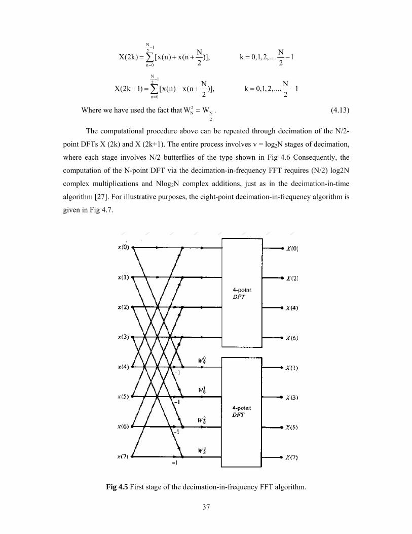
37
N 12
n 0
N NX(2k) [x(n) x(n )], k 0,1, 2,.... 12 2
−
=
= + + = −∑
N 12
n 0
N NX(2k 1) [x(n) x(n )], k 0,1, 2,.... 12 2
−
=
+ = − + = −∑
Where we have used the fact that 2N N
2
W W= . (4.13)
The computational procedure above can be repeated through decimation of the N/2-
point DFTs X (2k) and X (2k+1). The entire process involves v = log2N stages of decimation,
where each stage involves N/2 butterflies of the type shown in Fig 4.6 Consequently, the
computation of the N-point DFT via the decimation-in-frequency FFT requires (N/2) log2N
complex multiplications and Nlog2N complex additions, just as in the decimation-in-time
algorithm [27]. For illustrative purposes, the eight-point decimation-in-frequency algorithm is
given in Fig 4.7.
Fig 4.5 First stage of the decimation-in-frequency FFT algorithm.

38
Fig 4.6 Basic butterfly computation in the decimation-in-frequency.
Fig 4.7 N = 8-piont decimation-in-frequency FFT algorithm.
We observe from Fig 4.7 that the input data x (n) occurs in natural order, but the
output DFT occurs in bit-reversed order. We also note that the computations are performed in
place. However, it is possible to reconfigure the decimation-in-frequency algorithm so that
the input sequence occurs in bit-reversed order while the output DFT occurs in normal order
[28]. Furthermore, if we abandon the requirement that the computations be done in place, it is
also possible to have both the input data and the output DFT in normal order.
All data on microprocessors is stored in a binary representation at some level. ASCII
strings are represented by assigning 8 bits, or a byte, to each character in the string. You can
represent numerics in a variety of ways, but two representations have emerged as the standard

39
representations for decimal numbers floating-point and fixed-point. Each representation has
its advantages and disadvantages.
4.5 FLOATING-POINT REPRESENTATION The Institute of Electrical and Electronics Engineers (IEEE) standardizes floating-point
representation in IEEE 754. Floating-point representation is similar to scientific notation in
that there is a number multiplied by a base number raised to some power. For example,
118.625 is represented in scientific notation as 1.18625 x 10². The main benefit of this
representation is that it provides varying degrees of precision based on the scale of the
numbers. For example, it is beneficial to talk in terms of angstroms (10-10 m) when working
with the distance between atoms. However, dealing with the distance between cities, this
level of precision is no longer practical or necessary. IEEE 754 defines binary representations
for 32-bit single-precision and 64-bit double-precision (64-bit) numbers as well as extended
single-precision and extended double-precision numbers. Examine the specification for
single-precision, floating-point numbers, also called floats.
A float consists of three parts: the sign bit, the exponent, and the mantissa. The division of the three parts is as follows:
Fig.4.8 floating point representation
The sign bit is 0 if the number is positive and 1 if the number is negative. The exponent is an
8-bit number that ranges in value from -126 to 127. The exponent is actually not the typical
two's complement representation because this makes comparisons more difficult. Instead, the
value is biased by adding 127 to the desired exponent and representation, which makes it
possible to represent negative numbers.
The mantissa is the normalized binary representation of the number to be multiplied
by 2 raised to the power defined by the exponent. Now look at how to encode 118.625 as a
float. The number 118.625 is a positive number, so the sign bit is 0. To find the exponent and
mantissa, first write the number in binary, which is 1110110.101 (get more details on finding
this number in the "Fixed-Point Representation" section). Next, normalize the number to
1.110110101 x 26, which is the binary equivalent of scientific notation. The exponent is 6
and the mantissa is 1.110110101. The exponent must be biased, which is 6 + 127 = 133. The
binary representation of 133 is 10000101. Thus, the floating-point encoded value of 118.65 is

40
0100 0010 1111 0110 1010 0000 0000 0000. Binary values are often referred to in their
hexadecimal equivalent. In this case, the hexadecimal value is 42F6A000.
4.6 FIXED-POINT REPRESENTATION In fixed-point representation, a specific radix point - called a decimal point in English and
written "." is chosen so there is a fixed number of bits to the right and a fixed number of bits
to the left of the radix point. The bits to the left of the radix point are called the integer bits
[29]. The bits to the right of the radix point are called the fractional bits. In this example,
assume a 16-bit fractional number with 8 magnitude bits and 8 radix bits, which is typically
represented as 8.8 representations. Like most signed integers, fixed-point numbers are
represented in two's complement binary.
Fig 4.9 fixed point representation
Using a positive number keeps this example simple. To encode 188.625, first find the value
of the integer bits. The binary representation of 118 is 01110110, so this is the upper 8 bits of
the 16-bit number. The fractional part of the number is represented as 0.625 x 2n where n is
the number of fractional bits. Because 0.625 x 256 = 160, you can use the binary
representation of 160, which is 10100000, to determine the fractional bits. Thus, the binary
representation for 118.625 is 0111 0110 1010 0000. The value is typically referred to using
the hexadecimal equivalent, which is 76A0.
4.6.1 Unsigned fixed point:
Unsigned integers are represented in the binary number system in the following way. Let
b = [b (n) b (n-1) ... b (2) b (1)]
Be the binary digits of an n-bit unsigned integer, where each b (i) is either one or zero. Then
the value of b is u = b (n)*2^ (n-1) + b (n-1)*2^ (n-2) + ... + b (2)*2^ (1) + b (1)*2^ (0).
Unsigned fixed-point values are unsigned integers that are scaled by a power of two. We call
the negative exponent of the power of two the "fraction length”. If the unsigned integer u is
defined as before, and the fraction length is f, then the value of the unsigned fixed-point
number is uf = u*2^-f. let’s define the word length of a variable is 3 bits, fraction length is 1
bit, then the possible range of a variable is [0, 0.5, 1, 1.5, 2, 2.5, 3, 3.5] and the corresponding
binary representation is [000, 001, 010, 011, 100, 101, 110 ,111].if the word length is more
than this the dynamic range will be increased.

41
4.6.2 Signed fixed point:
Signed integers are represented in two’s-complements in the binary number system in the
following way. Let b = [b (n) b (n-1) ... b (2) b (1)] be the binary digits of an n-bit signed
integer, where each b (i) is either one or zero. Then the value of b is s = -b(n)*2^(n-1) + b(n-
1)*2^(n-2) + ... + b(2)*2^(1) + b(1)*2^(0).Note that the difference between this and the
unsigned number is the negative weight on the most-significant-bit (MSB).Signed fixed-point
values are signed integers that are scaled by a power of two . We call the negative exponent
of the power of two the "fraction length". If the signed integer s is defined as before, and the
fraction length is f, then the value of the signed fixed-point number is sf = s*2^-f.let’s define
the word length of a variable is 3 bits and fractional length is 1 bit. Then the possible range of
a variable is [-2,-1.5,-1,-0.5, 0, 0.5, 1, 1.5] and the corresponding binary representation is
[100,101,110,111,000,001,010,011].if the word length is more than this the dynamic range
will be increased.
The major advantage of using fixed-point representation for real numbers is that
fixed-point adheres to the same basic arithmetic principles as integers. Therefore, fixed-point
numbers can take advantage of the general optimizations made to the Arithmetic Logic Unit
(ALU) of most microprocessors, and do not require any additional libraries or any additional
hardware logic. On processors without a floating-point unit (FPU), such as the Analog
Devices Black fin Processor, fixed-point representation can result in much more efficient
embedded code when performing mathematically heavy operations.
In general, the disadvantage of using fixed-point numbers is that fixed-point numbers
can represent only a limited range of values, so fixed-point numbers are susceptible to
common numeric computational inaccuracies. For example, the range of possible values in
the 8.8 notation that can be represented is +127.99609375 to -128.0. So the addition of 100 +
100 will exceed the valid range of the data type, which is called overflow. In most cases, the
values that overflow are saturated, or truncated, so that the result is the largest representable
number. With fixed point design the dynamic range of numbers is a key concern since a
much narrower range of numbers can be represented in fixed format due to the fixed word
size. There are several different ways to represent a numerical value within a fixed length
binary word. This thesis primarily deals with fixed binary word lengths of 8 bits and 16 bits.
First, the algorithm is developed and simulated in double-precision floating-point. Second,
the algorithm is converted to fixed-point by changing the data type of the variables to fixed-
point.

42
4.6.3 Finite word length effects
Since DSP data must be represented by fixed point values with a finite number of bits there
are differences between an ideal (infinite precision) DSP system's performance and a real
world fixed point system. System error sources can include[30]:
Register overflow, or protected mode register saturation
Arithmetic errors (ex: feedback path error gain)
Coefficient representation errors (ex: coefficient accuracy truncation)
Finite word length effects add additional noise sources to the system. Primary quantization-
related sources of finite word length effects include:
Errors in arithmetic within the algorithm implementation (fixed point truncation)
Truncation error when results are stored (most DSP processors have extended registers
for holding arithmetic operation results, however truncation still occurs when results are
stored to memory)
Quantization of filter coefficients which must be stored in memory.
4.7 CONCLUSION: This chapter discussed about the radix-2 FFT decimation in time and decimation in frequency
algorithms in detail for 8- point FFT.it also discussed about fixed point and floating point
representations and their difference in representing a number by taking one example. it
discussed about the dynamic range of a fixed point variable based on the word length and
fraction lengths and the effects of finite word length .

Chapter 5
RESULTS & DISCUSSIONS
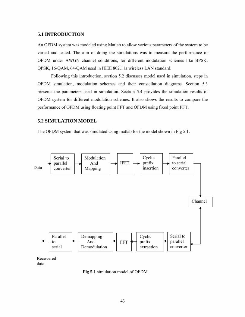
43
5.1 INTRODUCTION An OFDM system was modeled using Matlab to allow various parameters of the system to be
varied and tested. The aim of doing the simulations was to measure the performance of
OFDM under AWGN channel conditions, for different modulation schemes like BPSK,
QPSK, 16-QAM, 64-QAM used in IEEE 802.11a wireless LAN standard.
Following this introduction, section 5.2 discusses model used in simulation, steps in
OFDM simulation, modulation schemes and their constellation diagrams. Section 5.3
presents the parameters used in simulation. Section 5.4 provides the simulation results of
OFDM system for different modulation schemes. It also shows the results to compare the
performance of OFDM using floating point FFT and OFDM using fixed point FFT. 5.2 SIMULATION MODEL The OFDM system that was simulated using matlab for the model shown in Fig 5.1.
Fig 5.1 simulation model of OFDM
Serial to parallel converter
Modulation And Mapping
IFFT
Cyclic prefix insertion
Parallel to serial converter
Serial to parallel converter
FFT
Cyclic prefix extraction
Demapping And Demodulation
Parallel to serial
Channel
Data
Recovered data

44
5.2.1 Serial to Parallel Conversion
The input serial data stream is formatted into the word size required for transmission, e.g.
1 bit/word for BPSK, 2 bits/word for QPSK, 4bits/word for 16-QAM, 6 bits/word for 64-
QAM and shifted into a parallel format. The data is then transmitted in parallel by assigning
each data word to one carrier in the transmission.
5.2.2 Modulation schemes used in the simulation
Phase Shift Key (PSK) Modulation
With this method the phase of the carrier changes between different phases determined by the
logic states of the input bit stream. There are several different types of Phase Shift Key (PSK)
modulators. The PSK modulations used here are:
Two-Phase Shift Key Modulation
In this modulator the carrier assumes one of two phases. Logic 0 produces no phase change
and logic 1 produce a 180° phase change.
I-Q diagram
-1.5 -1 -0.5 0 0.5 1 1.5-1.5
-1
-0.5
0
0.5
1
1.5bpsk constellation diagram
Fig 5.2 BPSK constellation diagram
Four-Phase Shift Key Modulation
With 4 PSK or QPSK, 2 bits are processed to produce a single-phase change. In this case
each symbol consists of 2 bits.

45
I-Q Diagram
-1.5 -1 -0.5 0 0.5 1 1.5-1.5
-1
-0.5
0
0.5
1
1.5qpsk constellation diagram
Fig 5.3 QPSK constellation diagram
Quadrature amplitude modulation:
Quadrature Amplitude Modulation (QAM) is a modulation scheme in which both the phase
and amplitude of carrier is varied by the symbols of the message.Quadrature Amplitude
Modulation (QAM) is a combination of two modulation techniques: Amplitude Modulation
(AM) and Phase Modulation (PM). One convenient way to represent the possible states is to
use a constellation pattern diagram such as the below shown Figures. In this pattern we see
that the states are present at different amplitudes and phases. Dots are placed at the
constellation points. Whenever the amplitude or the phase changes, a new symbol is
transmitted.
16 QAM I-Q diagram:
-3 -2 -1 0 1 2 3
-3
-2
-1
0
1
2
3
16qam constellation diagram
Fig 5.4 16-QAM constellation diagram

46
64-QAM I-Q diagram:
Fig 5.5 64-QAM constellation diagram
Digital data is transferred in an OFDM link by using a modulation scheme on each subcarrier.
A modulation scheme is a mapping of data words to a real (In phase) and imaginary
(Quadrature) constellation, also known as an IQ constellation. For example 64-QAM
(quadrature amplitude modulation) has 64 IQ points in the constellation. The number of bits
that can be transferred using a single symbol corresponds to log2 (M), where M is the number
of points in the constellation, thus 64-QAM transfers bits per symbol. Each data word is
mapped to one unique IQ location in the constellation. The resulting complex vector I + j ×Q,
corresponds to an amplitude of √ (I2 + Q2) and a phase of (I + j ×Q) where j = -1.
Increasing the number of points in the constellation does not change the bandwidth of
the transmission, thus using a modulation scheme with a large number of constellation points,
allows for improved spectral efficiency.
However, the greater the number of points in the modulation constellation, the harder
they are to resolve at the receiver. As the IQ locations become spaced closer together, it only
requires a small amount of noise to cause errors in the transmission. This results in a direct
trade off between noise tolerance and the spectral efficiency of the modulation scheme and
was summarized by Shannon's Information Theory, which states that the maximum capacity
of a channel of bandwidth W, with a signal power of S, perturbed by white noise of average
power N, is given by
2SC W log (1 )N
= + (5.1)
The spectral efficiency of a channel is a measure of the number of bits transferred per second
for each Hz of bandwidth and thus the spectral efficiency SE is given by
-8 -6 -4 -2 0 2 4 6 8
-8
-6
-4
-2
0
2
4
6
8
64qam constellation diagram

47
E 2C SS log (1 )W N
= + (5.2)
5.2.3 Inverse fast Fourier Transform
After the required spectrum is worked out, an inverse fourier transform is used to find the
corresponding time waveform. The guard period is then added to the start of each symbol.
5.2.4 Guard Period
Guard period of length N/4 samples are cyclically appended at the start of each symbol,
where N is the FFT size.
5.2.5 Channel
A channel model is then applied to the transmitted signal. The model allows for the signal to
noise ratio, multipath to be controlled. The signal to noise ratio is set by adding a known
amount of white noise to the transmitted signal. Multipath delay spread then added by
simulating the delay spread using an FIR filter. The length of the FIR filter represents the
maximum delay spread, while the coefficient amplitude represents the reflected signal
magnitude.
5.2.6 Receiver
The receiver basically does the reverse operation to the transmitter. The guard period is
removed. The FFT of each symbol is then taken to find the original transmitted spectrum.
The phase angle of each transmission carrier is then evaluated and converted back to the data
word by demodulating the received phase. The data words are then combined back to the
same word size as the original data.
5.3 SIMULATION PARAMETERS
Following are the parameters used in simulation of OFDM system.
Parameter
value
modulations used BPSK,QPSK,16-QAM,64-QAM
FFT size 64
Number of carriers used 64
Guard time 16 samples
Guard period type Cyclic extension of the symbol
Table 5.1 OFDM simulation parameters

48
5.4 SIMULATION RESULTS All the simulation studies were conducted on a 2.80 GHz PC with 256 MB of RAM with
Microsoft windows XP operating system. All the simulations are done in matlab.Bit error rate
(BER) was considered as the performance index. IEEE 802.11a standard uses BPSK, QPSK,
16-QAM, 64-QAM modulations schemes for achieving different data rates. so, the BER
performance of OFDM for different modulation schemes like BPSK, QPSK,16-QAM, 64-
QAM were simulated against signal to noise ratio over an additive white Gaussian noise
channel. Low spectral efficiency modulation schemes, such as BPSK and QPSK, require a
lower SNR, and hence are more energy efficient. For a power limited system, with
unbounded bandwidth, the maximum data rate could be achieved using BPSK or QPSK.
However, in most applications the available bandwidth is the limiting factor and so the data
rate is maximised by using a more spectrally efficient modulation schemes such as 16-QAM,
64-QAM.
0 5 10 15 20 25 3010-4
10-3
10-2
10-1
100
SNR
BE
R
BER vs SNR
BPSKQPSK16-QAM64-QAM
Fig 5.6 BER vs. SNR plot for OFDM using BPSK, QPSK, 16-QAM, 64-QAM
Fig 5.6 presents the bit error rate performance of OFDM against SNR for different
modulation schemes The results shows that using QPSK, the transmission can tolerate a SNR
of >10-12dB. The bit error rate BER gets rapidly worse as the SNR drops below 6dB.

49
However, using BPSK allows the BER to be improved in a noisy channel, at the expense of
transmission data capacity. Using BPSK the OFDM transmission can tolerate a SNR of >6-
8dB. In a low noise link the capacity can be increased by using 16-QAM and 64-QAM.
Matlab simulations were used to examine the performance of OFDM using fixed
point transmitters and receivers incorporating IFFTs and FFTs, and were compared with the
performance of floating point FFT implementations. To understand the effect of fixed point
FFT design on overall system performance, we must take into account how the signals are
represented in fixed-point form at the input to the FFT.
First, the OFDM system was simulated for different modulation schemes like BPSK,
QPSK, 16-QAM, 64-QAM using floating point fast Fourier transform. These results are
shown in the Fig 5.6. Now floating point FFT was replaced by fixed point FFT. Fixed point
FFT was simulated for word lengths of 8 bit and 16 bit, assuming use of 8 bit and 16 bit DSP
processors. First it was simulated using fixed point FFT of input word length 8 bits, with this
it was not reaching floating point performance. Later the simulation was done by using fixed
point FFT of 16 bit word length.
Figure5.7and figure 5.8 shows the results from simulation of OFDM for BPSK
modulation using fixed point FFT with word length 8 bits. In the Fig 5.7, the BER
performance against SNR was evaluated for different combinations of integer part lengths
and fractional lengths of 2, 4, 6, and 0.in the Fig 5.8 the BER performance are compared for
varying size of integer and fractional lengths. The fractional lengths were varied from 0-7 bits.
This was done for Signal to noise ratio of 6db.
From Fig 5.8 it is seen that the receiver is not achieving floating point performance
for any combination of integer part lengths and fractional lengths.
Fig 5.9and Fig 5.10 shows the results from simulation of OFDM for QPSK
modulation using fixed point FFT with word length 8bits. In the Fig 5.9, the BER
performance against SNR was evaluated for different combinations of integer part lengths
and fractional lengths of 2,4, 6, and 0.in the Fig 5.10 the BER performance are compared for
varying size of integer and fractional lengths. The fractional lengths were varied from 0-7 bits.
This was done for Signal to noise ratio of 8db.
From Fig 5.10 it is seen that the receiver is not achieving floating point performance
for any combination of integer part lengths and fractional lengths.
In case of 16-QAM, 64-QAM the word length of 8 bits are not sufficient, there is
much difference between fixed point and floating point performance. that’s why those results
are not included here.
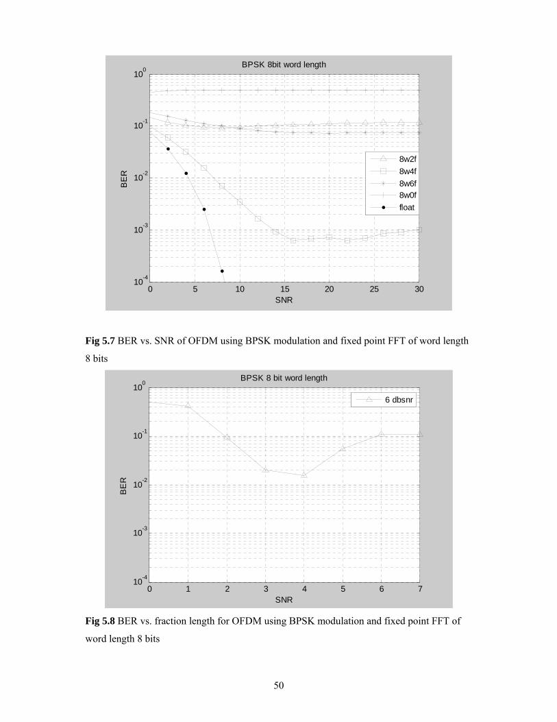
50
0 5 10 15 20 25 3010-4
10-3
10-2
10-1
100
SNR
BE
R
BPSK 8bit word length
8w2f8w4f8w6f8w0ffloat
Fig 5.7 BER vs. SNR of OFDM using BPSK modulation and fixed point FFT of word length
8 bits
0 1 2 3 4 5 6 710-4
10-3
10-2
10-1
100BPSK 8 bit word length
SNR
BE
R
6 dbsnr
Fig 5.8 BER vs. fraction length for OFDM using BPSK modulation and fixed point FFT of
word length 8 bits

51
0 5 10 15 20 25 3010-4
10-3
10-2
10-1
100QPSK 8 bit wordlength
SNR
BE
R
8w2f8w4f8w6f8w0ffloat
Fig 5.9 BER vs. SNR of OFDM using QPSK modulation and fixed point FFT of word length
8 bits
0 1 2 3 4 5 6 710-4
10-3
10-2
10-1
100QPSK 8bit word length
Fraction length
BE
R
8 db snr
Fig 5.10 BER vs. fraction length for OFDM using QPSK modulation and fixed point FFT of
word length 8 bits
52
Figure 5.11 and figure 5.12 shows the results from simulation of OFDM for BPSK
modulation using fixed point FFT with word length 16 bits. In the Fig 5.11, the BER
performance against SNR was evaluated for different combinations of integer part lengths
and fractional lengths of 6, 8, 10, and 12,14,0.in the Fig 5.12 the BER performance are
compared for varying size of integer and fractional lengths. The fractional lengths were
varied from 0-15 bits. This was done for Signal to noise ratio of 5db, 6db and 7db.
From Fig 5.12 it is seen that the receiver achieves floating point performance for 16-6,
16-8, and 16-10 sizes, and where 16 is the word length in bits and 6,8,10 are the fractional
lengths.
Figure5.13 and figure 5.14 shows the results from simulation of OFDM for QPSK
modulation using fixed point FFT with word length 16 bits. In the Fig 5.13, the BER
performance against SNR was evaluated for different combinations of integer part lengths
and fractional lengths of 6, 8, 10, and 12,14,0.in the Fig 5.14 the BER performance are
compared for varying size of integer and fractional lengths. The fractional lengths were
varied from 0-15 bits. This was done for Signal to noise ratio of 6db, 8db and 9db.
From Fig 5.14 it is seen that the receiver achieves floating point performance for 16-6,
16-8, and 16-10 sizes, and where 16 is the word length in bits and 6,8,10 are the fractional
lengths.
Fig 5.15 and Fig 5.16 shows the results from simulation of OFDM for 16-QAM
modulation using fixed point FFT with word length 16 bits. In the Fig 5.15, the BER
performance against SNR was evaluated for different combinations of integer part lengths
and fractional lengths of 6, 8, 10, and 12,14,0.in the Fig 5.16 the BER performance are
compared for varying size of integer and fractional lengths. The fractional lengths were
varied from 0-15 bits. This was done for Signal to noise ratio of 14db, 15db and 16db.
From Fig 5.16 it is seen that the receiver achieves floating point performance for 16-6,
16-8 sizes, and where 16 is the word length in bits and 6,8 are the fractional lengths.

53
0 5 10 15 20 25 3010
-4
10-3
10-2
10-1
100
SNR
BE
R
BPSK 16 bit wordlength
16w6f16w8f16w10f16w12f16w14f16w0ffloat
Fig 5.11 BER vs. SNR for OFDM using BPSK modulation and fixed point FFT of word
length 16 bits
0 5 10 1510-4
10-3
10-2
10-1
100
Fraction length
BE
R
BPSK 16 bit wordlength
5db snr6db snr7db snr
Fig 5.12 BERvs.fraction length of OFDM using BPSK modulation and fixed point FFT of
word length 16 bits

54
0 5 10 15 20 25 3010-4
10-3
10-2
10-1
100
SNR
BE
R
QPSK 16 bit word length
16w6f16w8f16w10f16w12f16w14f16w0ffloat
Fig 5.13 BER vs. SNR for OFDM using QPSK modulation and fixed point FFT of word
length 16 bits
0 5 10 1510-4
10-3
10-2
10-1
100
Fractionlength
BE
R
QPSK 16 bit wordlength
6db snr8 db snr9 db snr
Fig 5.14 BER vs. fraction length of OFDM using QPSK modulation and fixed point FFT of
word length 16 bits.

55
0 5 10 15 20 25 3010-4
10-3
10-2
10-1
100
SNR
BE
R
16-QAM 16 bitwordlength
16w6f16w8f16w10f16w12f16w14f16w0ffloat
Fig 5.15.BER vs. SNR for OFDM using 16-QAM modulation and fixed point FFT of word
length 16 bits
0 5 10 1510-4
10-3
10-2
10-1
100
Fractionlength
BE
R
16-QAM 16 bit wordlength
14dbsnr15dbsnr16dbsnr
Fig 5.16 BER vs. fraction length of OFDM using 16-QAM modulation and fixed point FFT
of word length 16 bits

56
0 5 10 15 20 25 3010-4
10-3
10-2
10-1
100
SNR
BE
R
64-QAM 16 bit word length
16w6f16w8f16w10f16w12f16w14f16w0ffloat
Fig 5.17 BER vs. SNR for OFDM using 64-QAM modulation and fixed point FFT of word
length 16 bits
0 5 10 1510-4
10-3
10-2
10-1
100
Fractionlength
BE
R
64-QAM 16bit wordlength
20dbsnr21db snr22dbsnr
Fig 5.18 BER vs. fraction length of OFDM using 64 -QAM modulation and fixed point FFT
of word length 16 bits.

57
Figure5.17and figure 5.18 shows the results from simulation of OFDM for 64-QAM
modulation using fixed point FFT with word length 16 bits. In the Fig 5.17, the BER
performance against SNR was evaluated for different combinations of integer part lengths
and fractional lengths of 6, 8, 10, and 12,14,0.in the Fig 5.18 the BER performance are
compared for varying size of integer and fractional lengths. The fractional lengths were
varied from 0-15 bits. This was done for Signal to noise ratio of 20db, 21db and 22 db.
From Fig 5.18 it is seen that the receiver achieves floating point performance for 16-6,
16-8 sizes, and where 16 is the word length in bits and 6, 8 are the fractional lengths.
5.5 CONCLUSION Varieties of simulations are conducted to measure the effects of finite word length on the
performance of OFDM system. From these simulations, it is seen that the input word length
of 8 bits is not sufficient to achieve the best BER performance with respect to floating point
FFT. It is also observed that the word length of 16 bits is sufficient to achieve the best BER
performance. Fixed point FFT provides nearly same performance to floating point FFT by
selecting proper integer part lengths and fractional part lengths.

Chapter 6
CONCLUSIONS

58
6.1 INTRODUCTION The current status of the research is that OFDM appears to be a suitable technique as a
modulation technique for high performance wireless telecommunications. In this thesis An
OFDM link has been confirmed to work by using computer simulations. The effect of
additive white Gaussian noise on OFDM system was observed. In this thesis 64- point
IFFT/FFT was used in the OFDM system. The effects of fixed point FFT were observed on
the performance of OFDM system and compared with the performance of OFDM using
floating point FFT.The effects of fixed point FFT were tested for word lengths of 8bits and
16 bits. It was observed that word length of 8 bits is not sufficient to achieve floating point
performance. In the case of input word length of 16 bits, observed the best combination of
integer part length and fractional part length which can achieve the performance of OFDM
when using floating point FFT.
6.2 ACHIEVEMENT OF THE THESIS
From the variety of simulation studies conducted, it is seen that word length of 8 bits
is not sufficient to achieve best BER performance with respect to floating point performance
for any combination of integer part lengths and fractional part lengths. In case of input word
length of 16 bits, it is seen that fixed point FFT provides nearly similar performance to
floating point FFT if the delay parameter is suitably selected. Again it also seen that fraction
part of half the size of word length provides the best performance, the performance remains
same near this fractional part size.
6.3 LIMITATIONS OF THE THESIS
AWGN channel only considered.
Inter symbol interference is not considered.
Scaling is not done.
Matlab simulations are taking more simulation time for OFDM using fixed point than
OFDM using floating point.
Base band simulation only considered.

59
6.4 SCOPE OF FURTHER RESEARCH
Simulations can be extended to 24 bit, 32 bit word lengths.
FPGA implementation of OFDM can also be investigated.
Effect of ISI, fading can also be considered on the performance of OFDM system.
Scaling can also be considered to avoid overflows.

60
REFERENCES
[1] R. R. Mosier and R. G. Clabaugh, “Kineplex, a bandwidth-efficient binary transmission
system”, IEEE Transactions, Vol. 76, January 1958, pp. 723 – 728.
[2] Robert Chang, “Orthogonal frequency division multiplexing”, US. Patent 3,488445, filed
November 14, 1966, issued January 6, 1970.
[3] Robert Chang, “Synthesis of Band-Limited Orthogonal Signals for Multichannel Data
Transmission”, the Bell System Technical Journal, December 1966, pp. 1775 -1796.
[4] S. B. Weinstein, Paul M. Ebert, “Data Transmission by Frequency-Division Multiplexing
Using the Discrete Fourier Transform”, IEEE Transactions on Communication Technology,
Vol. COM-19, No. 5, October 1971, pp. 628 – 634.
[5] Louis Thibault, Minh Thien Le, “Performance Evaluation of COFDM for Digital Audio
Broadcasting Part I: Parametric Study”, IEEE Transactions on Broadcasting, Vol. 43, No.1,
March 1997, pp. 64 – 75
[6] Ulrich Reimers, “Digital Video Broadcasting”, IEEE Communications Magazine, June
1998, pp. 104 - 110
[7] ETSI EN 300 421, “Framing Structure, channel coding and modulation for 11/12 GHz
satellite services”, August 1997, pp. 6, Online: http://www.etsi.org
[8] ETSI ETS 300 744, “Framing Structure, Channel Coding and Modulation for Digital
Terrestrial Television”, March 1997, online: http://www.etsi.org
[9] M. Johnsson, “HiperLAN/2 – The Broadband Radio Transmission Technology
Operating in the 5 GHz Frequency Band”,
Online: http://www.hiperlan2.com/site/specific/specmain/specwh.htm, 1999
[10] Yiyan Wu, William Y. Zou, “Orthogonal Frequency Division Multiplexing: A Multi
Carrier Modulation Scheme”, IEEE Transaction on Consumer Electronics, Vol. 41, No. 3,
August 1995, pp. 392 - 399
[11] Wickelgren, I.J,”Local-area networks go wireless”, Spectrum IEEE Volume 33, Issue
9, Sept. 1996 Page(s):34 – 40.
[12] Sicher, A,” HiperLAN/2 and the evolution of wireless LANs”IEEE transactions On
Emerging technologies symposium: broadband, wireless internet access, 2000, 10-11 April
2000 Page(s):1 pp.
[13] R. Van Nee et al. New high-rate wireless LAN standards. IEEE Communications
Magazine, 40:140OE147, January 2002.

61
[14] Yiyan Wu, William Y. Zou, “Orthogonal Frequency Division Multiplexing: A
MultiCarrier Modulation Scheme”, IEEE Transaction on Consumer Electronics, Vol. 41,
No.3, August 1995, pp. 392 – 399.
[15] S. A. Fechtel,’’ OFDM: From the Idea to Implementation”, Advances in Radio Science -
Kleinheubacher Berichte, Copernicus GmbH publishers, 2005.
Online:http://www.adv-radio-sci.net/3/27/2005/ars-3-27-2005.pdf
[16] Comsa, C.; Bogdan, I,”system level design of baseband OFDM for wireless LAN”,
International symposium on signals, circuits and systems, 2003.SCS 2003, Volume 1, 10- 11
July 2003 Page(s):313 - 316 vol.1.
[17] R. van Nee, “A new OFDM standard for high rate wireless LAN in the 5 GHz band,”
Proceedings of the IEEE Vehicular Technology Conference, pp. 258–262, 1999.
[18] White Paper: High-speed wireless OFDM communication systems, Wi-LAN Inc.,
February 2001.
[19] Xiaodong Wang,”OFDM and its application to 4G”, international conference on
Wireless and optical communications, 2005.14 Th annual WOCC 2005.
[20] J.H. Stott,’’The how and why of COFDM”, tutorial, BBC Research and Development
[21] Sun, Y,” bandwidth efficient wireless OFDM “, IEEE journal on selected areas in
Communications, Volume 19, Issue 11, Nov. 2001 Page(s):2267 – 2278.
[22] Aguado, L.E.; Wong, K.K.; O'Farrell, T,”Coexistence issues for 2.4 GHz OFDM
WLANs”third international conference on (conf.publ.no.489) 3G mobile communication
Technologies, 2002 page(s):400-404
[23] Jain, M.; Roja, M.M,” Comparison of OFDM with CDMA system in wireless
telecommunication for multipath delay spread”, the first IEEE and IFIP international
coference in central asia on internet,2005, 26-29 Sept. 2005 Page(s):5 pp.
[24] Eric lawrey,” Adaptive Techniques for Multiuser OFDM”,
http://www.skydsp.com/resources/OFDM_thesis_lawrey.PDF,Dec2001.
[25] Van Nee Richard, and Prasad Ramjee,”OFDM for Wireless Multimedia
Communications” Boston: ArtechHouse, 2000.
[26] Sadat, A.; Mikhael, W.B.” Fast Fourier Transform for high speed OFDM wireless
multimedia system, Proceedings of the 44th IEEE 2001 Midwest Symposium on circuits and
systems,2001, Volume 2, 14-17 Aug. 2001 Page(s):938 - 942 vol.2
[27] Jizhong Han; Gang Ren; Chengde Han,’’ A novel fixed-point FFT algorithm on
embedded digital signal processing systems”, 5 Th international conferences on signal

62
Processing proceedings, 2000, WCCC-ICSP2000, Volume 1, 21-25 Aug. 2000 Page(s):48 –
53 vol.1.
[28] Khan, A.U.; Al-Akaidi, M.M.; Khan, S.A.; Khattak, S.; Mir, A,” Performance analysis
of a 64-point FFT/IFFT block designed for OFDM technique used in WLANs”, 7 Th
international multi topic conference-2003(INMIC 2003), 8-9 Dec. 2003 Page(s):65 – 71.
[29] Welch, P,”a fixed point fast Fourier transform analysis”, IEEE transactions on audio
and electro acoustics, Volume 17, Issue 2, Jun 1969 Page(s):151 – 157.
[30] Armstrong, J.; Suraweera, H. A.; Brewer, S.; Slaviero, R,’’ Effect of rounding and
saturation in fixed-point DSP implementation of IFFT and FFT for OFDM applications”, The
Embedded Signal Processing Conference (GSPx 2004), September 2004.