Effects of Discount Rate and Various Costs on Optimal ...s-space.snu.ac.kr/bitstream/10371/67633/3/Paper-D-09-00052.pdf · 2 distance, expected total lifetime cost, optimal design

1

Manuscript No. KSCE-D-09-00052

Effects of Discount Rate and Various Costs on Optimal Design of

Caisson Breakwater

Kyung-Duck Suh*, Kyung-Suk Kim

**, and Deok-Lae Kim

***

Abstract

In this study, the method developed by Goda and Takagi in 2000 for optimal design of a

vertical breakwater caisson is extended to take into account the effects of discount rate

and economic damage costs due to long-term harbor shutdown and temporal stoppage of

harbor operation. The effect of discount rate is important only at smaller return periods

where the damage to the caisson frequently occurs. Among the various costs, the initial

construction cost and the economic damage cost due to long-term harbor shutdown

caused by extraordinary sliding of caissons are found to be equally important in finding

the minimum expected total lifetime cost. On the other hand, the rehabilitation cost and

the economic damage cost due to temporal stoppage of harbor operation caused by

excessive wave overtopping are not so important in the optimal design of the breakwater.

In general, in smaller water depths the optimal return period and the corresponding

optimal cross-section of the caisson are determined as those yielding the minimum

expected total lifetime cost, while they are determined by the allowable expected sliding

distance in greater water depths.

Keywords: breakwaters, caissons, discount rate, economic damage cost, expected sliding

* Member, Professor, Dept. of Civil and Environmental Engineering, Seoul National University, 599

Gwanangno, Gwanak-gu, Seoul 151-744, Korea (Corresponding Author, E-mail: [email protected]) **

Member, Researcher, Research Center for Waterfront and New Ocean Energy Development, Kwandong

University, 522 Naegok-dong, Gangneung-si, Gangwon-do 210-701, Korea (E-mail:

[email protected]) ***

Member, Graduate Student, Dept. of Civil and Environmental Engineering, Seoul National University,

Seoul 151-744, Korea; presently, Hyundai Institute of Construction Technology, Hyundai Engineering &

Construction Co., Ltd., 102-4 Mabuk-dong, Giheung-gu, Yongin-si, Gyunggi-do 446-716, Korea (E-mail:

[email protected])

mailto:[email protected]

2

distance, expected total lifetime cost, optimal design

1. Introduction

Vertical breakwaters, along with rubble mound breakwaters, have been widely used

to provide a calm basin for ships and to protect harbor facilities from rough seas,

especially where the water depth is relatively large. The current deterministic design

method is well established for not only the resistance of the upright section against

sliding and overturning but also the bearing capacity of the rubble mound foundation and

the seabed. In the deterministic design method, uncertainties in the magnitudes of

loading on and resistance of the structure are supposed to be covered by a safety factor.

Therefore, it is difficult to consider the uncertainties of each design parameter separately

and to evaluate the relative importance of different failure modes, so that there is always

a possibility to over- or under-design the structure. To overcome these shortcomings of

the deterministic design, the reliability-based design method has been proposed. For a

vertical breakwater, Burcharth and Sørensen (2000) established a partial safety factor

system by summarizing the results of the PIANC (Permanent International Association

of Navigation Congresses) Working Group 28, which was adopted by U.S. Army Corps

of Engineers (2002) as well. This system belongs to what is called as Level 2 methods.

On the other hand, performance-based design methods have also been developed, in

which the expected sliding distance of a caisson of a vertical breakwater during its

lifetime is estimated (Shimosako and Takahashi, 2000; Hong et al., 2004).

In order to properly apply the reliability-based design method, the probabilistic and

statistical characteristics of the variables involved in the design should be known. The

level of acceptable probability of failure (in Level 2 method) or expected sliding distance

(in performance-based design method) of the caisson should also be specified a priori. A

method being used to determine the acceptable probability of failure is to calculate the

probability of failure of existing breakwaters that were constructed by the deterministic

design method but did not suffer significant damage for a long time. Assuming that these

breakwaters have enough reliability, the acceptable probability of failure may be taken as

either the failure probability of the breakwaters or a somewhat smaller value. The same

principle could be used for the acceptable expected sliding distance of a caisson.

However, this method can be subjective in certain cases, because the sample breakwaters

3

were designed and constructed neither in the same condition nor with the same safety

level.

Recently, to cope with this problem, efforts are made to introduce the concept of

optimization in the design of breakwaters, which considers their functionality and

economics as well as their safety.

In the optimal design of a breakwater, it is designed so that the total lifetime cost

(including initial construction cost, maintenance cost, rehabilitation and economic

damage costs, and so on) becomes a minimum, while it fulfills a certain level of safety

necessary for maintaining its functionality. In the case of a vertical breakwater, Burcharth

et al. (1995) formulated a reliability-based design optimization procedure, in which the

objective function models the cost of the caisson which is assumed to be proportional to

the width of the caisson. The only design variable considered was the caisson width,

though reliability analyses were made for sliding of the caisson, foundation failure in the

rubble mound and rupture failure in clay. They assumed a specific water depth at the site.

With the limited water depth it was not relevant with a high foundation as it would have

caused larger wave impacts.

Voortman et al. (1998) proposed a more realistic procedure, in which the objective

function consists of two parts that describe the construction costs and the expected costs

of failure, respectively. Moreover, as design variables, the caisson height, the caisson

width and the height of the rubble foundation were considered.

In the above-mentioned optimization studies, Level 2 methods were used in the

reliability analyses. Recently, Goda and Takagi (2000) extended the performance-based

design method of Shimosako and Takahashi (2000) by introducing the concept of the

optimal return period for selection of design wave heights, and proposed a method to

determine the optimal cross-section of a caisson that yields the minimum expected total

lifetime cost within the allowable expected sliding distance. More recently, Burcharth

and Sørensen (2006) used a similar approach by taking into account not only caisson

sliding but also slip failure in rubble foundation and repair by placing mounds in front or

behind the caisson.

In the present study, we extend Goda and Takagi’s (2000) model by taking into

account the interest cost and the long-term change of the monetary values by inflation

and others. Furthermore, the economic damage costs due to long-term harbor shutdown

caused by extraordinary sliding of caissons and temporal stoppage of harbor operation

4

due to excessive wave overtopping are also considered.

In the following section, the method for calculating the expected total lifetime cost is

described. In Sec. 3, the procedure for determining the optimum cross-section of the

caisson is described. In Sec. 4, some calculation examples are presented to examine the

effects of discount rate, economic damage costs and water depth. In Sec. 5, sensitivity

analyses are made for the discount rate and the criterion of caisson sliding distance for

harbor shutdown. The major conclusions then follow.

2. Calculation of Expected Total Lifetime Cost

The total lifetime cost consists of the initial construction cost, rehabilitation cost, and

economic damage costs due to long-term harbor shutdown or temporal stoppage of

harbor operation. The maintenance costs are neglected in this paper because they are

usually small compared with other costs. Many of the parameters for calculation of

various costs are borrowed from Voortman (1998) with some modifications.

2.1 Initial Construction Cost

To calculate the initial construction cost, the length and cross-section of the

breakwater and the costs of construction materials should be known. The total length of

the breakwater is assumed to be 3,000 meters. The material costs used are 200 and 250

US$/m3 for caisson and rubble mound, respectively, which are the values presently used

in Korea.

2.2 Rehabilitation Cost

There are several modes of failure for vertical caisson breakwaters. Goda and Takagi

(2000) examined the failure modes of the caisson breakwaters constructed in Japan over

several tens of years, and concluded that the sliding of caissons comprises the majority

of the cases of breakwater damage. Therefore, the sliding of the caisson is taken as the

principal and only failure mode of vertical breakwaters in the present study. The

Japanese breakwaters have low rubble mounds in general. The failure of rubble mound

could also be important for caissons placed on high rubble mounds. Therefore, the

present analysis and results may be limited to caissons placed on relatively low rubble

mound over a strong seabed.

5

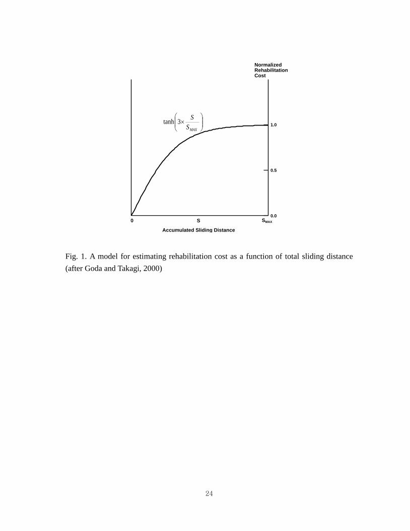
Goda and Takagi (2000) also proposed three simple models to estimate the

rehabilitation cost, in which the rehabilitation cost increases with the sliding distance

linearly, parabolically, or tangent-hyperbolically. Once the rehabilitation work starts, a

great initial cost may be needed without regard to the sliding distance. Therefore, we

adopted the third model as shown in Fig. 1, in which the cost increases rapidly with the

sliding distance when the sliding distance is relatively small, and the rate of increase is

reduced as the sliding distance increases. The model shown in Fig. 1 computes the

rehabilitation cost, no matter how small the sliding distance is. In the present study,

however, we introduced the threshold distance of 0.3 m, below which no rehabilitation

work is made. The cost of rehabilitation normalized with the initial construction cost is

then given by

MAX

MAX

MAX

r

SS

SSS

S

S

C

,1

3.0,3tanh

m3.0,0

(1)

where S is the accumulated sliding distance in meters, and MAXS is the threshold

sliding distance beyond which the caisson is judged as fallen from the mound and is

given by

2

BbSMAX (2)

where b is the rear berm width of rubble mound foundation and B is the caisson

width. Finally, the rehabilitation cost is calculated by multiplying the normalized cost

rC by the initial construction cost.

2.3 Economic Damage Cost Due to Harbor Shutdown

Even though the rehabilitation work should be made when the accumulated sliding

distance exceeds 0.3 m, the breakwater still could maintain its function until the caisson

6

slides much farther so that the harbor completely loses its function and is shutdown. In

order to calculate the economic damage cost due to harbor shutdown, the accumulated

sliding distance for harbor shutdown and the resulting economic cost should be

determined.

Takahashi et al. (2001) defined the accumulated sliding distance of 1.0 m as the

collapse limit state in which extremely large sliding occurs such that the caisson falls off

the rubble mound foundation. This value could be used as the criterion of sliding

distance for harbor shutdown. However, it seems somewhat unreasonable to use 1.0 m

without regard to the caisson width. In the present study, therefore, we recommend to use

MAXS1.0 as the criterion for harbor shutdown. According to the results of the present

study, in the case where the water depth is 20 m and the design significant wave height is

7~8 m, MAXS is calculated to be about 15 m. Therefore, the sliding distance for harbor

shutdown is 1.5 m, which is not much different from 1.0 m proposed by Takahashi et al.

(2001) as the collapse limit state. The smaller the water depth and wave height become,

the smaller becomes MAXS , so that MAXS1.0 will be closer to 1.0 m. MAXS in Eq. (2)

was derived only in the geometrical viewpoint by assuming that the rubble mound is

rigid and the pressures on the front and rear sides of the caisson are the same as the

hydrostatic pressure. In the real situation where waves act on the caisson which is

mounted on a rubble mound of granular material, the caisson may fall from the mound at

a sliding distance much smaller than MAXS . Note that MAXS used as the criterion for

caisson fall in Eq. (2) is only to calculate the rehabilitation cost using Eq. (1).

To calculate the economic damage cost due to harbor shutdown, a socio-economic

analysis should be made. In this study, however, we just adopted the value used by

Vrijling et al. (2000), US$ 555 million per event. This value originated from a similar

study for a rubble mound breakwater (Delft University of Technology, 1995).

2.4 Economic Damage Cost Due to Temporal Stoppage of Harbor Operation

When wave overtopping is so severe that the transmitted waves agitate the inside of

the harbor beyond a certain level, the harbor operation will be stopped temporarily. The

threshold wave heights for cargo handling should be determined in consideration of the

type, size, and cargo handling characteristics of the vessels. Overseas Coastal Area

Development Institute of Japan (2002) recommends the significant wave height of 0.5 m

as the threshold wave height for cargo handling for medium- and large-sized vessels. In

7

the present study, we adopted this value as the criterion of transmitted wave height for

temporal stoppage of harbor operation.

The wave transmission coefficient due to wave overtopping is calculated by

XX

i

Xc

XX

i

XX

Xc

X

i

c

X

t

H

h

h

dd

H

h

h

dd

H

h

C

1

11

22

1

for101.0

for

101.02

sin125.0

(3)

where ch is the crest elevation, h the water depth in front of the breakwater, d the

depth above the armor layer of the rubble foundation, cd the vertical distance from the

bottom of the caisson to the top of the armor layer of the rubble foundation, and iH is

the incident wave height, which was taken as the daily maximum significant wave height

in the present study. The preceding equation was proposed by Heijn (1997) by adding

the new variables X , X , and X to Goda’s (1969) model so that it can be used for

different types of caissons. We used 9.0X , 34.0X , and 0X proposed

for a conventional caisson. We also used 2.21 and the value of given in the

Goda’s (1969) report as a function of hd / .

The wave height inside the harbor is calculated by multiplying the daily maximum

significant wave height iH by the wave transmission coefficient tC . If the calculated

wave height is greater than 0.5 m, it is assumed that the harbor operation is stopped on

that day. This may lead to an overestimation of the stoppage time. However, such an

assumption is used because the economic damage cost is given per day. The waves

diffracted through the harbor entrance are neglected, and the transmitted wave over the

structure is assumed to directly influence the vessels at anchor. The economic damage

cost due to stoppage of harbor operation is taken as US$ 750,000 per day, again by

following Vrijling et al. (2000).

2.5 Conversion to Present Value

8

The above-mentioned rehabilitation cost and economic damage costs are the costs

which will occur in the future and in different times in general. The monetary value

changes with time. Therefore it is necessary to convert the costs to those at a certain

reference time. It is customary to take the time of initial construction cost as the present

time and convert all the future costs to those in the present time. To convert the future

monetary value to the present value, the future cost is multiplied by the present value

interest factor, i.e.

L

nn

n

r

CPV

1 1 (4)

where PV is the present value of the future costs, nC the cost which will occur after

n years, nr)1/(1 the present value interest factor, r the real discount rate, and L

is the service lifetime of the breakwater. The real discount rate is calculated by

jij

ir

1

1

1 (5)

where i is the nominal discount rate, and j is the inflation rate. In principle, the

nominal discount rate is taken as the interest rate of long-term treasury bonds, but the

bank interest rate is often used when the share of the bonds is not so great as to dominate

the rate of interest.

Different discount rates are used depending on the importance and service lifetime of

structures; the longer service lifetime, the lower discount rate, in general. In the present

study, the real discount rate of 3.7% was used, which was calculated using the average

values of the inflation rates and interest rates provided by Korea National Statistical

Office and the Bank of Korea, respectively, for seven years from 1999 till 2005. The

service lifetime of the breakwater was taken as 50 years.

3. Procedure of Optimal Design

In this paper, fictitious design cases are considered. However, the deepwater wave

condition is assumed to be the same as that used by Kim and Suh (2006) for Donghae

9

Harbor breakwater located in the east coast of Korea. The cumulative probability

distribution of the extreme wave height is given by the Weibull distribution:

1.1

493.1

037.3exp1

XXF (6)

where X stands for the annual maximum significant wave height. The wave periods

are calculated by the relationship proposed by Goda (2001) as 63.0

03.3 ss HT , where

0sH and sT are the deepwater significant wave height and period, respectively. The

significant wave heights for the return periods of 50 and 100 years are 8.2 and 9.0 m,

respectively, and the corresponding wave periods are 12.4 and 13.2 s.

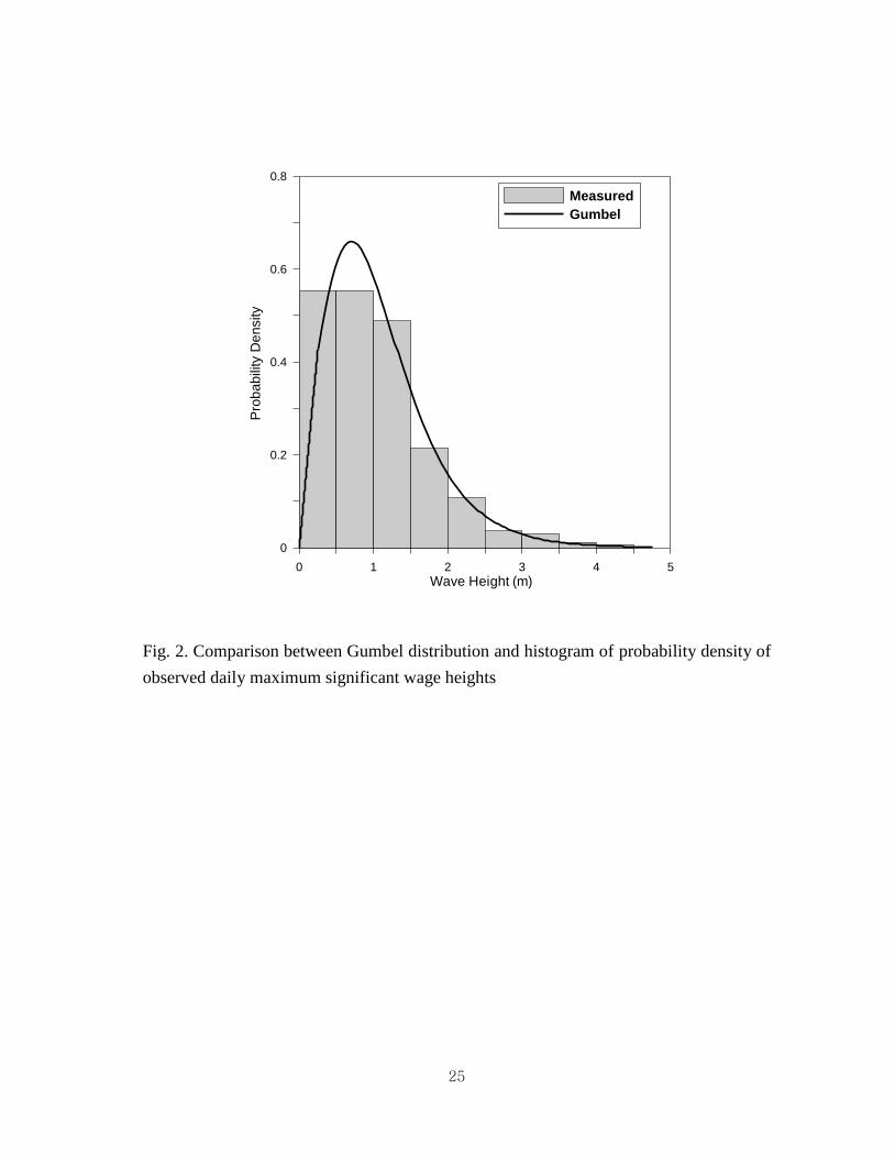
In order to calculate the economic damage cost due to temporal stoppage of harbor

operation, the cumulative probability distribution of the ordinary wave heights should be

known. For this, we used the wave data observed by Korea Ministry of Marine Affairs &

Fisheries (2001) for one year of 2000 at Gangneung wave observation station, which is

close to Donghae Harbor. We assume that the wave data observed in 2000 represent the

average wave climate in this area and the distribution of daily wave heights is the same

in other years. The histogram of the probability density of the observed daily maximum

significant wave heights are shown in Fig. 2, along with the Gumbel distribution whose

parameters were estimated using the method of moments:

56.0

7.0expexp

xxF (7)

where x indicates the daily maximum significant wave height.

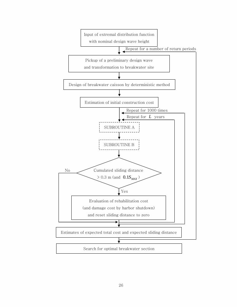
The procedure for optimal design of the caisson is explained in conjunction with the

computational flow chart sketched in Fig. 3. First, using the extreme wave height

distribution function given by Eq. (6) and the nominal design wave height with the return

period of 50 years, a preliminary design wave height is picked up. The preliminary wave

height is varied over a certain range by choosing the return period in a range of 0.5 to 2.0

10

times the service lifetime. If the optimal caisson design is not obtained within this range

of wave height, then the range is expanded until the optimum design is obtained.

The variation of water level by tides, t , is represented with a triangular distribution,

which extends from LWL ( 0t ) to HWL ( t ), where is the tidal range. The

effect of storm surge is also taken into account by adding 10% of the deepwater wave

height to the tide level.

Once the offshore wave height, wave period, and water level are determined, the

significant wave height at the location of the breakwater is calculated. In the present

study, we assumed unidirectional random waves propagating normal to the shoreline on a

plane beach of slope of 1/100. For this, we used Kweon et al.’s (1997) wave

transformation model by setting the directional spreading parameter maxs to be 1,000.

The variability in principal wave direction was not considered. For the calculated wave

height, the caisson is designed according to the conventional deterministic design

method with the safety factor of 1.2, and the initial construction cost is calculated.

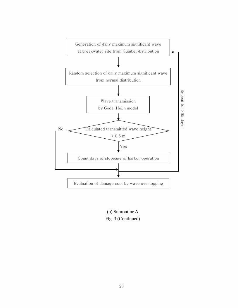
The designed caisson is then subjected to simulated daily maximum waves over one

year as shown in Fig. 3(b) Subroutine A. For each simulated daily maximum wave, the

transmitted wave height is calculated by Eq. (3). If the transmitted wave height is greater

than 0.5 m, it is assumed that the harbor operation is stopped on that day. The number of

these days is counted during the 365 days of calculation, and it is used for the estimation

of economic damage cost due to temporal stoppage of harbor operation for one year. This

procedure is repeated for L years to obtain the expected cost.

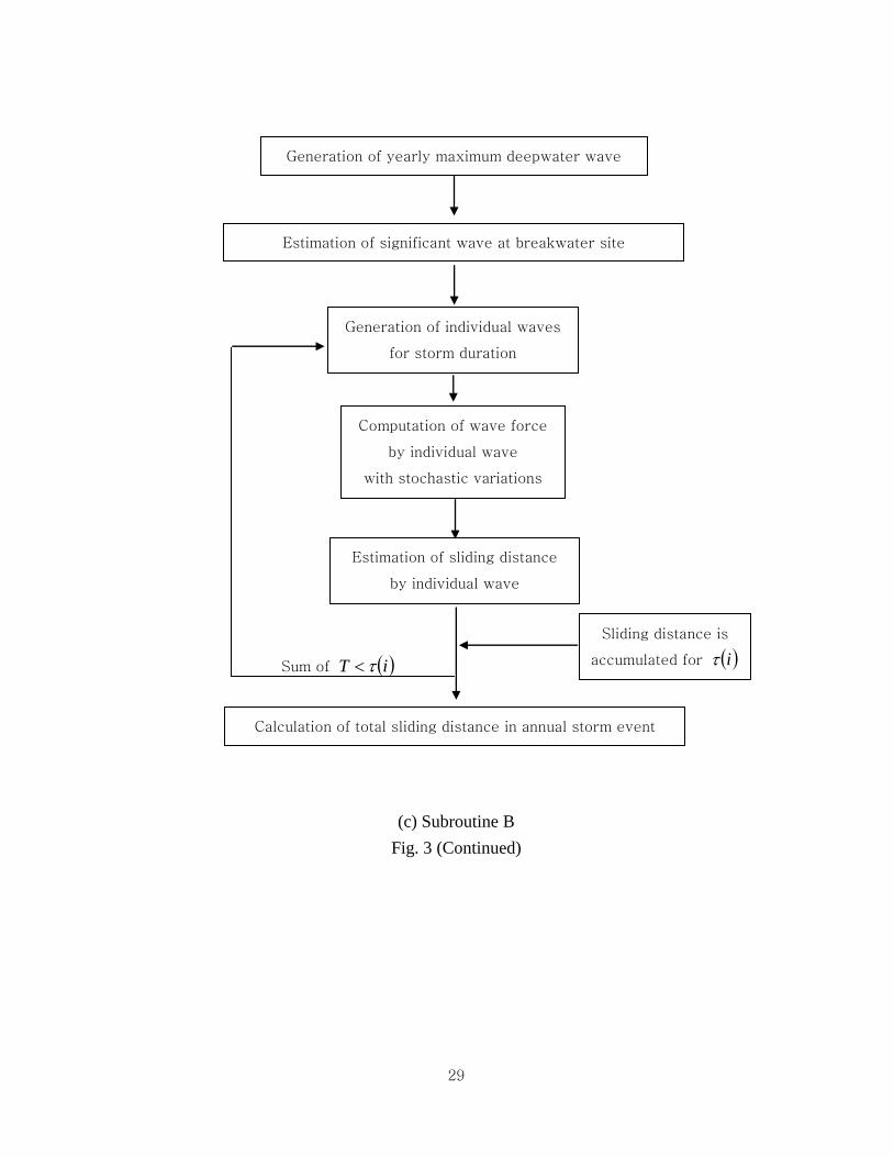
The designed cross section of caisson is also subjected to simulated yearly storm

waves over L years. In general, the sliding of a caisson is caused by large waves

comparable to the design waves. Therefore, the annual maximum wave height is

considered sufficient to be incorporated into the calculation. For each simulated yearly

storm, the total sliding distance is calculated. The process of this calculation is the same

as that of Hong et al. (2004) and briefly represented as Fig. 3(c) Subroutine B. In the

figure, T is the wave period of an individual wave and is the storm duration, which

was taken as 2 hours in this study. Goda and Takagi (2000) evaluated the rehabilitation

cost on the basis of accumulated sliding distance for L years, because they did not take

into account the discount rate and the economic damage cost due to harbor shutdown. In

order to take these into consideration, however, it is important to find when the

rehabilitation work is needed and when the harbor shutdown occurs. In the present study,

11

the values of total sliding distance by yearly storms are accumulated, and if the

accumulated value becomes greater than 0.3 m, the rehabilitation cost is calculated by Eq.

(1) and the sliding distance is reset to zero. If the accumulated sliding distance is greater

than MAXS1.0 , both the rehabilitation cost and economic damage cost due to harbor

shutdown are calculated.

The process of L -year cycles is repeated 1,000 times, and the total lifetime costs

and accumulated sliding distances thus obtained are added together to yield the expected

values of total cost and sliding distance. This process is repeated for a number of return

periods of different design wave heights. Finally, the cross-section of the caisson that

yields the minimum expected total lifetime cost within the allowable expected sliding

distance is searched. The corresponding return period is then the optimal return period.

To reduce the number of simulations (i.e. 1,000 times) in Fig. 3(a), the Latin

hypercube sampling technique (McKay et al., 1979) was used. To briefly explain this

technique, consider a variable Y that is a function of other random variables

kXXX ,,, 21 . The Latin hypercube sampling selects L different values from each of

k variables kXXX ,,, 21 in the following manner. The range of each variable is

divided into L non-overlapping intervals on the basis of equal probability. One value

from each interval is selected at random with respect to the probability density in the

interval. The L values thus obtained for 1X are paired in a random manner (equally

likely combinations) with the L values of 2X . These L pairs are combined in a

random manner with the L values of 3X to form L triplets, and so on, until L k -

tuplets are formed. This is the Latin hypercube sample. The Latin hypercube sampling

can be used when the variables are independent. In the present study, therefore, only the

annual maximum wave height, friction coefficient between caisson and rubble mound,

and the water level were sampled using the Latin hypercube sampling, while the

conventional random sampling was used for other variables, in the calculation of sliding

distance due to yearly storm waves. On the other hand, the Latin hypercube sampling

was used for the daily maximum wave height and water level in the calculation of

transmitted wave heights due to wave overtopping.

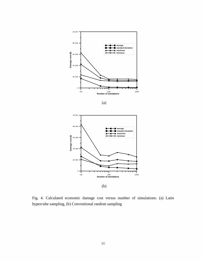
Fig. 4 shows the relation between the number of simulations and the expected

damage cost (due to harbor shutdown and temporal stoppage of harbor operation)

calculated with the Latin hypercube sampling and conventional random sampling. The

design wave height of return period of 50 years and the water depth of 19 m at the design

12

site were used. In Fig. 4 are shown the maximum, minimum, and average values of 10

calculation results of the expected damage cost obtained for the respective number of

simulations along with the standard deviation. Assuming that the coefficient of variation

(i.e. standard deviation divided by average) must be less than 0.1, about 1,000

simulations are enough if the Latin hypercube sampling is used, but the conventional

approach shows the coefficient of variation greater than 0.2 even for the number of

simulations of 10,000.

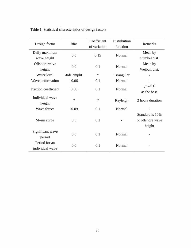
In Table 1 are given the design factors employed in the present study and their

statistical characteristics, which were obtained based on Goda and Takagi (2000) and

Hong et al. (2004).

The procedure explained above can be mathematically expressed as minimizing the

cost function given by

M

r

zFNCzFNCzFNCzIzI

M

m

L

nn

n

OO

n

SS

n

R

n

R

1 1

)()()()(

01

(8)

where z

is the vector of design variables (crest elevation and caisson width), zI

expected total lifetime cost, zI

0 initial construction cost, )(n

RC rehabilitation cost in

the n-th year, SC economic damage cost due to harbor shutdown per event, OC

economic damage cost due to temporal stoppage of harbor operation per day, zFNn

R

)(

number of rehabilitation in the n-th year (0 or 1), zFNn

S

)( number of harbor shutdown

in the n-th year (0 or 1), zFNn

O

)( number of days of stoppage of harbor operation in

the n-th year, and M is the number of simulations (1,000 in the present study).

4. Illustrative Examples

In principle, the economic optimization of a breakwater is performed in such a way

that the total lifetime cost is minimized. However, there can be a case in which the

13

breakwater is damaged too many times during its lifetime if the breakwater is designed

by the economic optimization principle alone. Therefore, we have to satisfy both the

economic optimization and the condition to keep the expected damage below a tolerable

limit. In this study, the optimal cross-section of a caisson is defined as the cross-section

which yields the minimum expected total lifetime cost within the allowable expected

sliding distance by following Goda and Takagi (2000). In the case where the point of

minimum cost is not found within the allowable sliding distance, the cross-section at the

allowable expected sliding distance is defined as the optimal cross-section. The

allowable expected sliding distance has been proposed as 0.3 and 0.1 m respectively by

Shimosako and Takahashi (2000) and Goda and Takagi (2000). In the present study,

both of these are examined.

The breakwater is assumed to be installed parallel to the shoreline on a plane beach

of slope of 1/100. Constant values were used for the height of the rubble mound from the

seabed to the bottom of the caisson of 2.5 m, the height of foot-protection block and

armor layer of the mound of 1.5 m, and the front and rear berm widths of the mound of

10 and 7 m, respectively. The crest elevation of the caisson was taken as sc Hh 6.0 ,

where sH is the design significant wave height at the location of the breakwater.

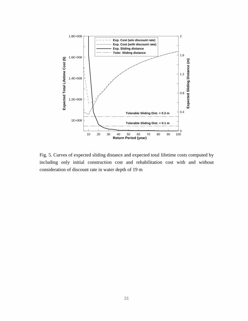
4.1 Effect of Discount Rate

In order to examine the effect of the discount rate, we included only the initial

construction cost and the rehabilitation cost with or without consideration of the discount

rate in the calculation, neglecting the economic damage costs. Fig. 5 compares the

expected total lifetime costs with respect to the return period calculated with and without

consideration of the discount rate in water depth of 19 m. The right ordinate indicates the

expected sliding distance. The difference becomes undistinguishable as the return period

increases because the cross-section of the caisson enlarges with the return period so that

little damage occurs and consequently the effect of the discount rate disappears. The

return period of the minimum total cost is 10 years in both cases, but the corresponding

expected sliding distance is much greater than the allowable ones.

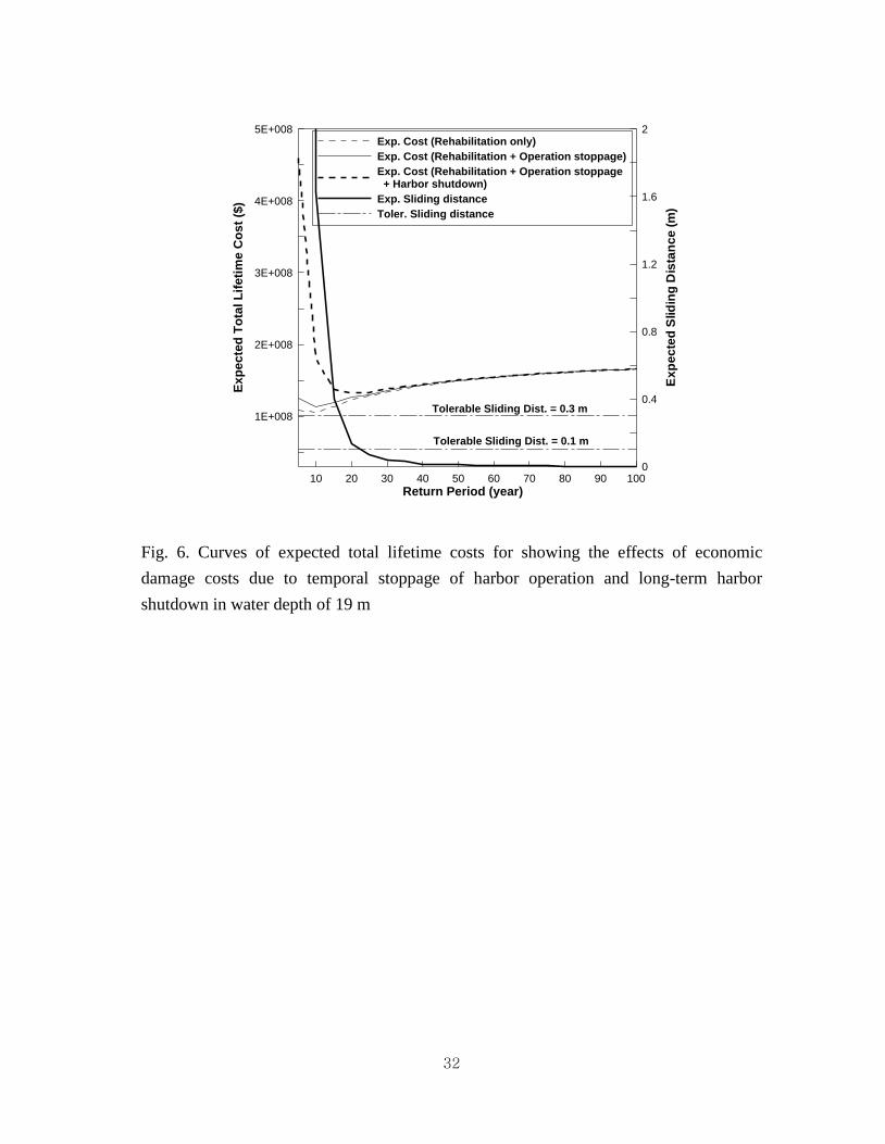
4.2 Effects of Economic Damage Costs

Fig. 6 shows the expected total lifetime costs calculated by including (1) only the

rehabilitation cost, (2) the rehabilitation cost and the economic damage cost due to only

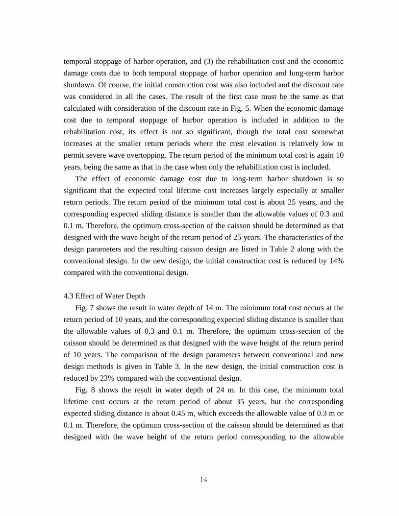
14

temporal stoppage of harbor operation, and (3) the rehabilitation cost and the economic

damage costs due to both temporal stoppage of harbor operation and long-term harbor

shutdown. Of course, the initial construction cost was also included and the discount rate

was considered in all the cases. The result of the first case must be the same as that

calculated with consideration of the discount rate in Fig. 5. When the economic damage

cost due to temporal stoppage of harbor operation is included in addition to the

rehabilitation cost, its effect is not so significant, though the total cost somewhat

increases at the smaller return periods where the crest elevation is relatively low to

permit severe wave overtopping. The return period of the minimum total cost is again 10

years, being the same as that in the case when only the rehabilitation cost is included.

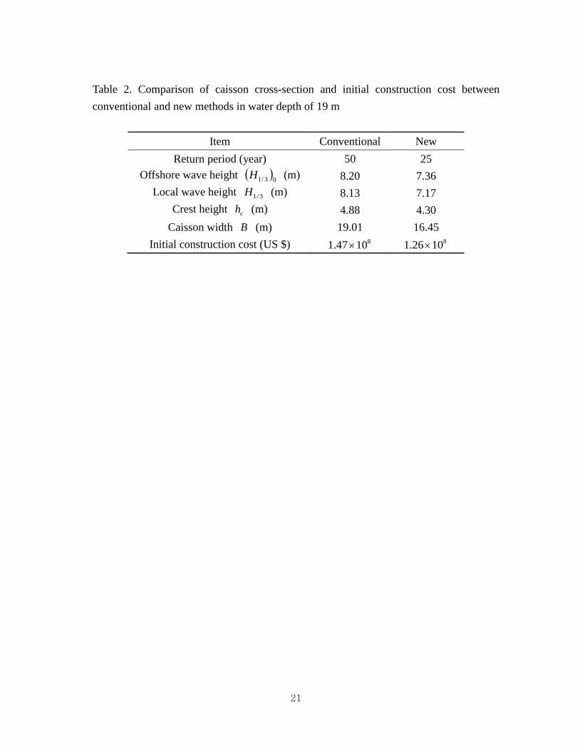
The effect of economic damage cost due to long-term harbor shutdown is so

significant that the expected total lifetime cost increases largely especially at smaller

return periods. The return period of the minimum total cost is about 25 years, and the

corresponding expected sliding distance is smaller than the allowable values of 0.3 and

0.1 m. Therefore, the optimum cross-section of the caisson should be determined as that

designed with the wave height of the return period of 25 years. The characteristics of the

design parameters and the resulting caisson design are listed in Table 2 along with the

conventional design. In the new design, the initial construction cost is reduced by 14%

compared with the conventional design.

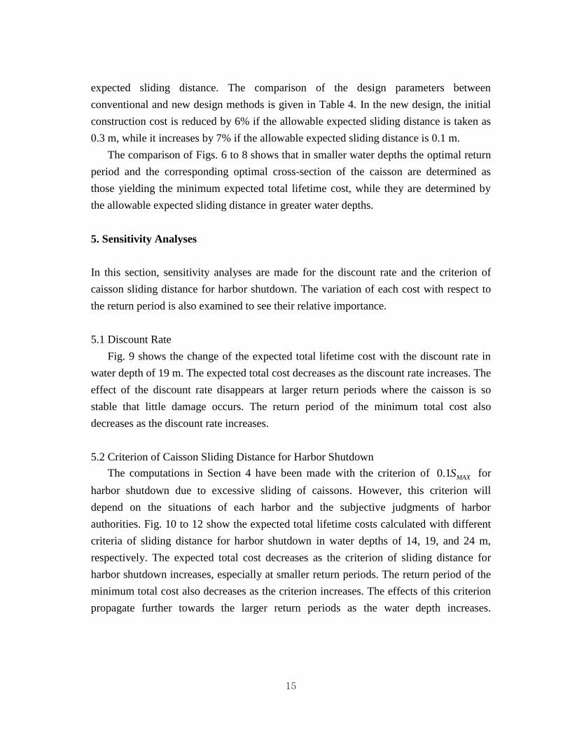
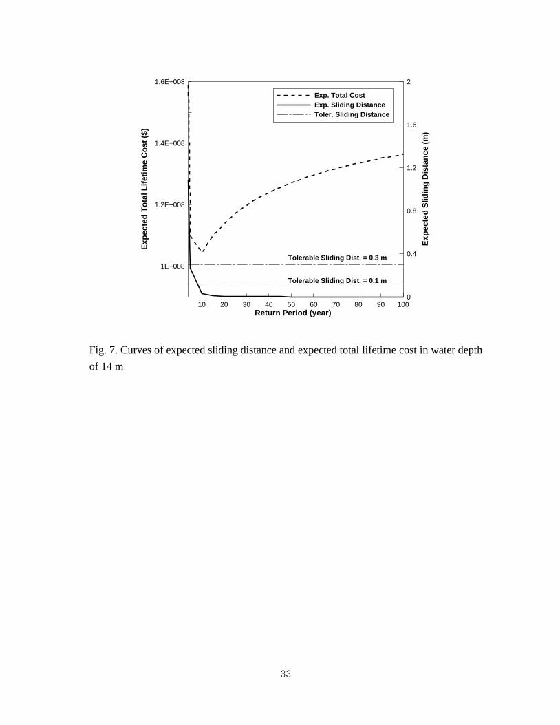
4.3 Effect of Water Depth

Fig. 7 shows the result in water depth of 14 m. The minimum total cost occurs at the

return period of 10 years, and the corresponding expected sliding distance is smaller than

the allowable values of 0.3 and 0.1 m. Therefore, the optimum cross-section of the

caisson should be determined as that designed with the wave height of the return period

of 10 years. The comparison of the design parameters between conventional and new

design methods is given in Table 3. In the new design, the initial construction cost is

reduced by 23% compared with the conventional design.

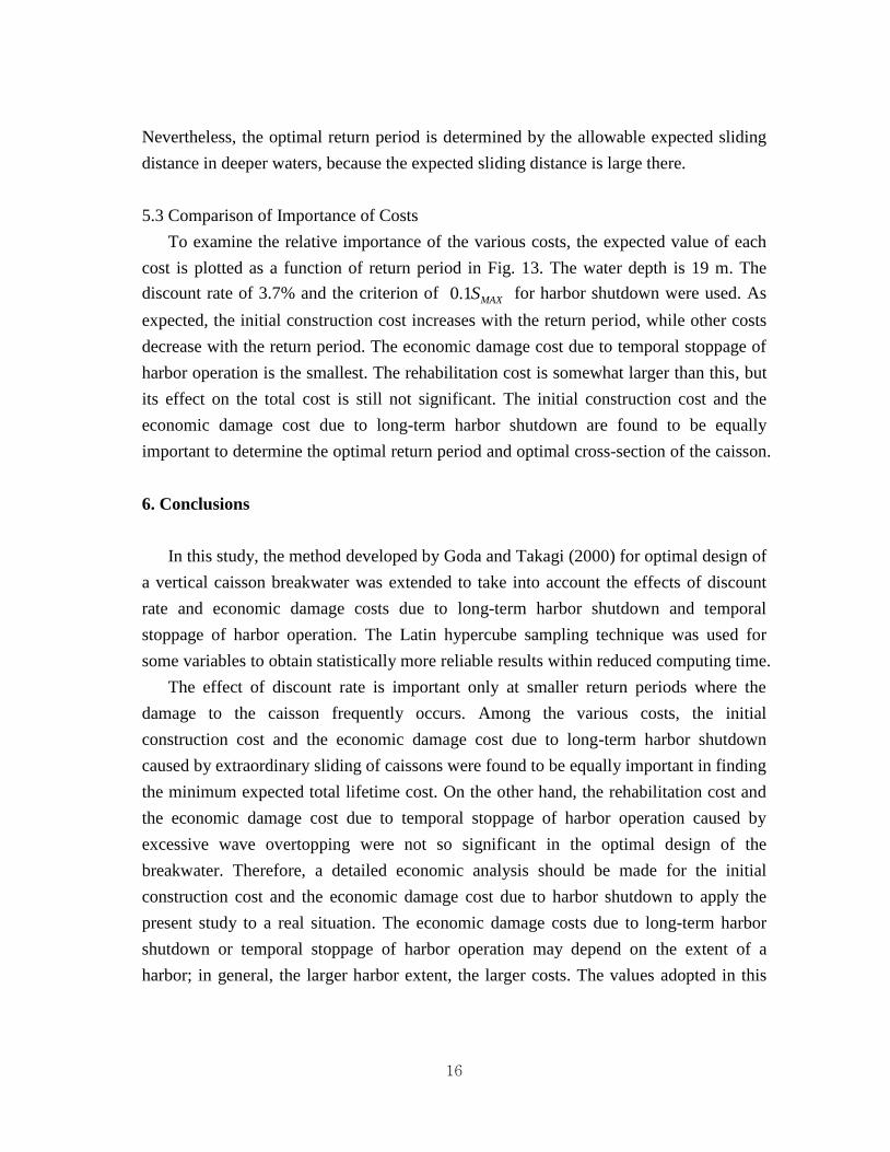
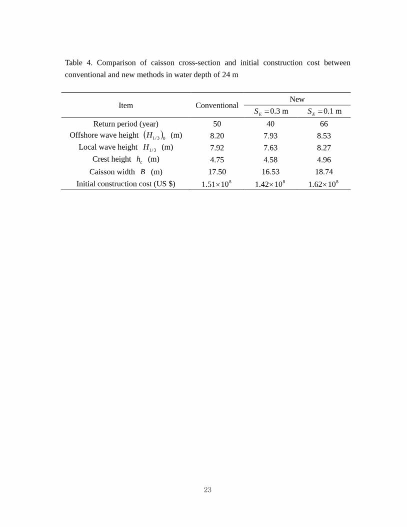
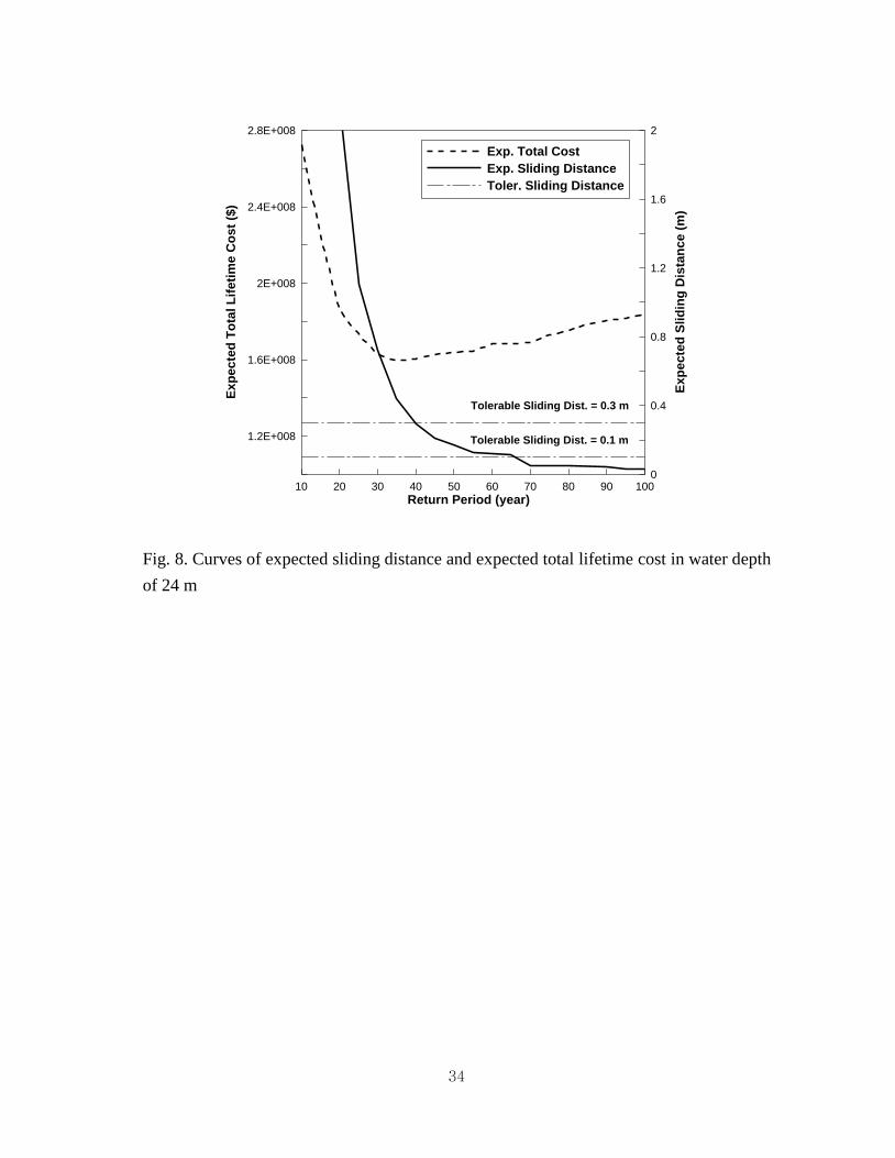
Fig. 8 shows the result in water depth of 24 m. In this case, the minimum total

lifetime cost occurs at the return period of about 35 years, but the corresponding

expected sliding distance is about 0.45 m, which exceeds the allowable value of 0.3 m or

0.1 m. Therefore, the optimum cross-section of the caisson should be determined as that

designed with the wave height of the return period corresponding to the allowable

15

expected sliding distance. The comparison of the design parameters between

conventional and new design methods is given in Table 4. In the new design, the initial

construction cost is reduced by 6% if the allowable expected sliding distance is taken as

0.3 m, while it increases by 7% if the allowable expected sliding distance is 0.1 m.

The comparison of Figs. 6 to 8 shows that in smaller water depths the optimal return

period and the corresponding optimal cross-section of the caisson are determined as

those yielding the minimum expected total lifetime cost, while they are determined by

the allowable expected sliding distance in greater water depths.

5. Sensitivity Analyses

In this section, sensitivity analyses are made for the discount rate and the criterion of

caisson sliding distance for harbor shutdown. The variation of each cost with respect to

the return period is also examined to see their relative importance.

5.1 Discount Rate

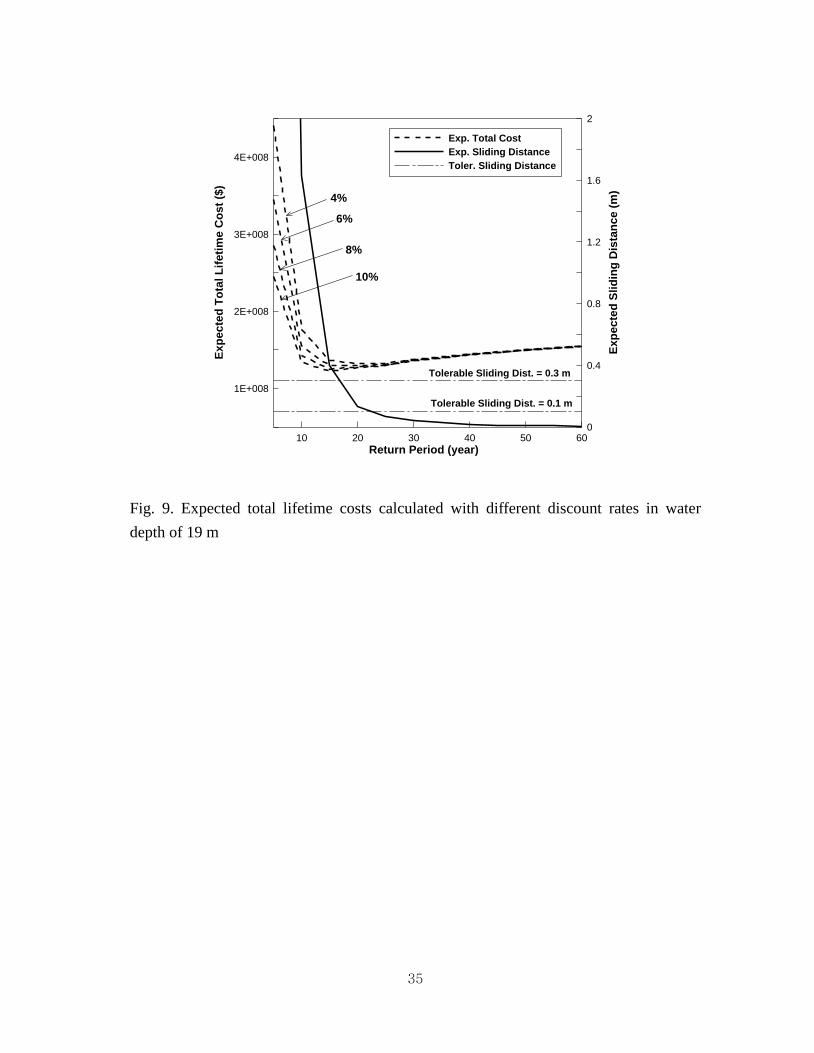
Fig. 9 shows the change of the expected total lifetime cost with the discount rate in

water depth of 19 m. The expected total cost decreases as the discount rate increases. The

effect of the discount rate disappears at larger return periods where the caisson is so

stable that little damage occurs. The return period of the minimum total cost also

decreases as the discount rate increases.

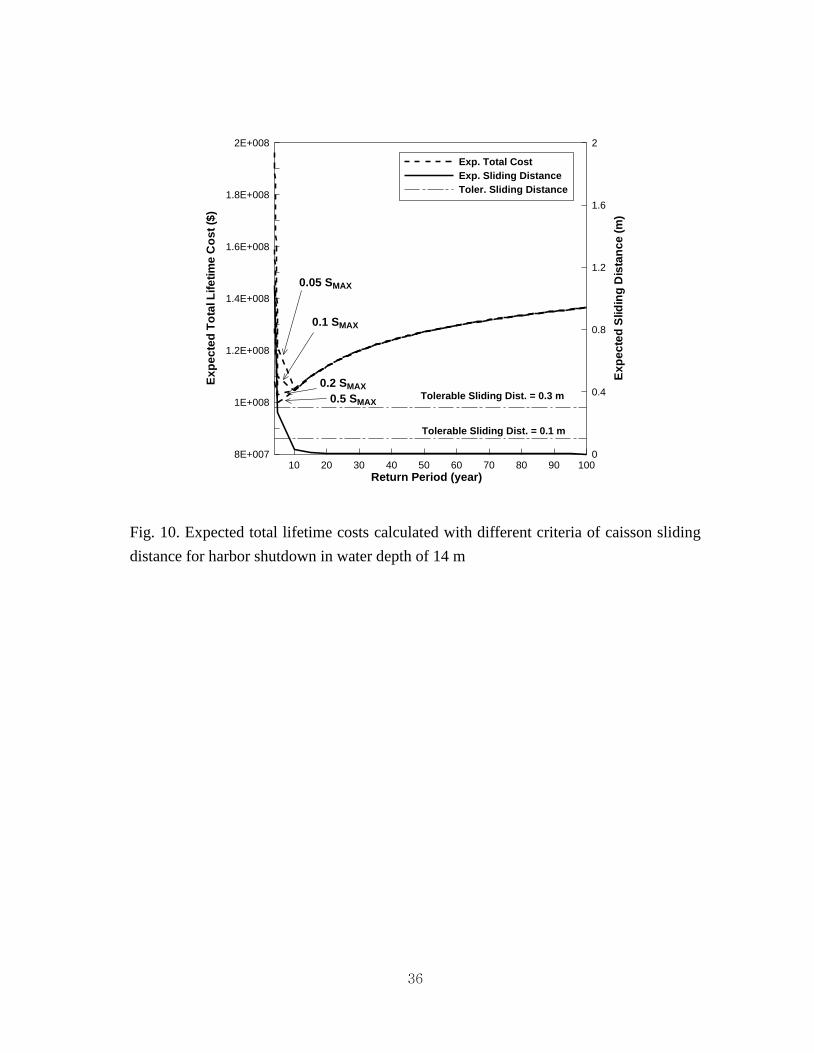
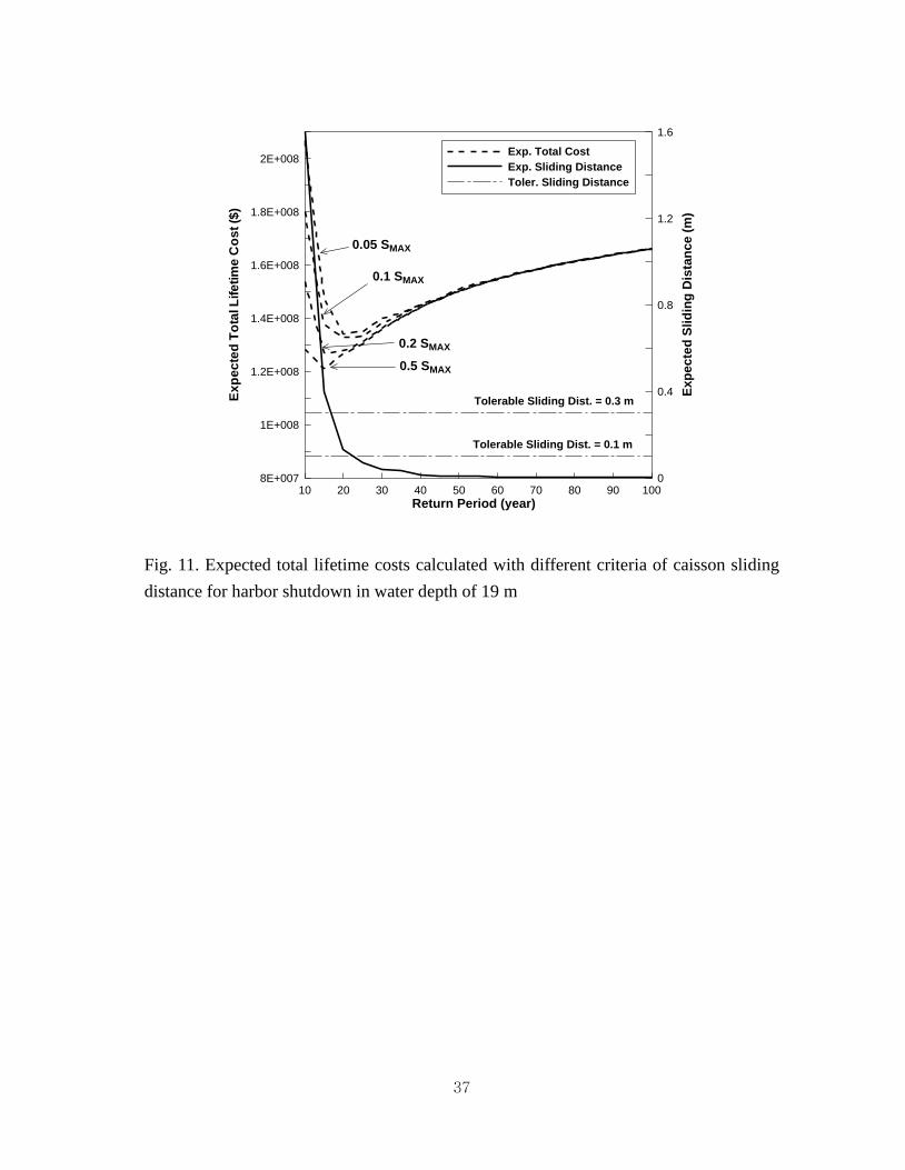
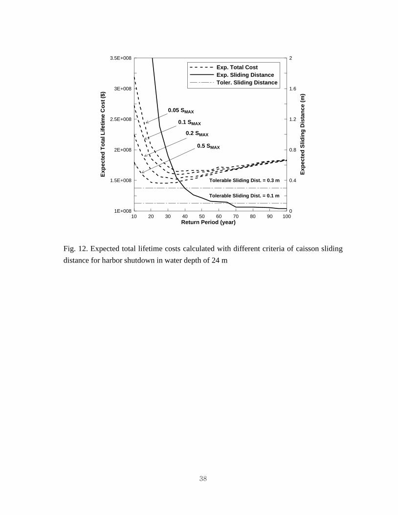
5.2 Criterion of Caisson Sliding Distance for Harbor Shutdown

The computations in Section 4 have been made with the criterion of MAXS1.0 for

harbor shutdown due to excessive sliding of caissons. However, this criterion will

depend on the situations of each harbor and the subjective judgments of harbor

authorities. Fig. 10 to 12 show the expected total lifetime costs calculated with different

criteria of sliding distance for harbor shutdown in water depths of 14, 19, and 24 m,

respectively. The expected total cost decreases as the criterion of sliding distance for

harbor shutdown increases, especially at smaller return periods. The return period of the

minimum total cost also decreases as the criterion increases. The effects of this criterion

propagate further towards the larger return periods as the water depth increases.

16

Nevertheless, the optimal return period is determined by the allowable expected sliding

distance in deeper waters, because the expected sliding distance is large there.

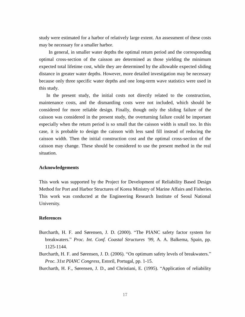
5.3 Comparison of Importance of Costs

To examine the relative importance of the various costs, the expected value of each

cost is plotted as a function of return period in Fig. 13. The water depth is 19 m. The

discount rate of 3.7% and the criterion of MAXS1.0 for harbor shutdown were used. As

expected, the initial construction cost increases with the return period, while other costs

decrease with the return period. The economic damage cost due to temporal stoppage of

harbor operation is the smallest. The rehabilitation cost is somewhat larger than this, but

its effect on the total cost is still not significant. The initial construction cost and the

economic damage cost due to long-term harbor shutdown are found to be equally

important to determine the optimal return period and optimal cross-section of the caisson.

6. Conclusions

In this study, the method developed by Goda and Takagi (2000) for optimal design of

a vertical caisson breakwater was extended to take into account the effects of discount

rate and economic damage costs due to long-term harbor shutdown and temporal

stoppage of harbor operation. The Latin hypercube sampling technique was used for

some variables to obtain statistically more reliable results within reduced computing time.

The effect of discount rate is important only at smaller return periods where the

damage to the caisson frequently occurs. Among the various costs, the initial

construction cost and the economic damage cost due to long-term harbor shutdown

caused by extraordinary sliding of caissons were found to be equally important in finding

the minimum expected total lifetime cost. On the other hand, the rehabilitation cost and

the economic damage cost due to temporal stoppage of harbor operation caused by

excessive wave overtopping were not so significant in the optimal design of the

breakwater. Therefore, a detailed economic analysis should be made for the initial

construction cost and the economic damage cost due to harbor shutdown to apply the

present study to a real situation. The economic damage costs due to long-term harbor

shutdown or temporal stoppage of harbor operation may depend on the extent of a

harbor; in general, the larger harbor extent, the larger costs. The values adopted in this

17

study were estimated for a harbor of relatively large extent. An assessment of these costs

may be necessary for a smaller harbor.

In general, in smaller water depths the optimal return period and the corresponding

optimal cross-section of the caisson are determined as those yielding the minimum

expected total lifetime cost, while they are determined by the allowable expected sliding

distance in greater water depths. However, more detailed investigation may be necessary

because only three specific water depths and one long-term wave statistics were used in

this study.

In the present study, the initial costs not directly related to the construction,

maintenance costs, and the dismantling costs were not included, which should be

considered for more reliable design. Finally, though only the sliding failure of the

caisson was considered in the present study, the overturning failure could be important

especially when the return period is so small that the caisson width is small too. In this

case, it is probable to design the caisson with less sand fill instead of reducing the

caisson width. Then the initial construction cost and the optimal cross-section of the

caisson may change. These should be considered to use the present method in the real

situation.

Acknowledgements

This work was supported by the Project for Development of Reliability Based Design

Method for Port and Harbor Structures of Korea Ministry of Marine Affairs and Fisheries.

This work was conducted at the Engineering Research Institute of Seoul National

University.

References

Burcharth, H. F. and Sørensen, J. D. (2000). “The PIANC safety factor system for

breakwaters.” Proc. Int. Conf. Coastal Structures ’99, A. A. Balkema, Spain, pp.

1125-1144.

Burcharth, H. F. and Sørensen, J. D. (2006). “On optimum safety levels of breakwaters.”

Proc. 31st PIANC Congress, Estoril, Portugal, pp. 1-15.

Burcharth, H. F., Sørensen, J. D., and Christiani, E. (1995). “Application of reliability

18

analysis for optimal design of monolithic vertical wall breakwaters.” Proc. Int. Conf.

Coastal and Port Engineering in Developing Countries, Rio de Janeiro, Brazil, pp.

1321-1336.

Delft University of Technology (1995). Ennore Coal Project, India. Risk analysis and

probabilistic modeling, Delft.

Goda, Y. (1969). Re-analysis of laboratory data on wave transmission over breakwaters,

Rep. of Port and Harbour Res. Inst., Vol. 8, No. 3, pp. 3-18.

Goda, Y. (2001). “Performance-based design of caisson breakwaters with new approach

to extreme wave statistics,” Coastal Engrg. J., 43(4), 289-316.

Goda, Y. and Takagi, H. (2000). “A reliability design method of caisson breakwaters

with optimal wave heights,” Coast. Engrg. J., Vol. 42, No. 4, pp. 357-387.

Heijn, K. M. (1997). Wave transmission at vertical breakwaters, Afstudeerverslag,

Technishe Universiteit Delft, Faculteit Civiele Techniek.

Hong, S. Y., Suh, K. D., and Kweon, H.-M. (2004). “Calculation of expected sliding

distance of breakwater caisson considering variability in wave direction,” Coast.

Engrg. J., Vol. 46, No. 1, pp. 119-140.

Kim, S.-W. and Suh, K.-D. (2006). “Application of reliability design methods to

Donghae Harbor breakwater,” Coast. Engrg. J., Vol. 48, No. 1, pp. 31-57.

KMOMAF (2001). Korea Ministry of Marine Affairs & Fisheries, Ocean Wave

Observation, Analysis and Prediction (in Korean).

Kweon, H.-M., Sato, K., and Goda, Y. (1997). “A 3-D random breaking model for

directional spectral waves,” Proc. 3rd Int. Symp. Ocean Wave Measurement and

Analysis, ASCE, Norfolk, pp. 416-430.

McKay, M. D., Beckman, R. J., and Conover, W. J. (1979). “A comparison of three

methods for selecting values of input variables in the analysis of output from a

computer code,” Technometrics, Vol. 21, No. 2, pp. 239-245.

OCADIJ (2002). Overseas Coastal Area Development Institute of Japan, Technical

Standards and Commentaries for Port and Harbor Facilities in Japan.

Shimosako, K. and Takahashi, S. (2000). “Application of deformation-based reliability

design for coastal structures,” Proc. Int. Conf. Coastal Structures ’99, A. A. Balkema,

Spain, pp. 363-371.

Takahashi, S., Shimosako, K., and Hanzawa, M. (2001). “Performance design for

maritime structures and its application to vertical breakwaters―Caisson sliding and

19

deformation-based reliability design,” Proc. Int. Workshop on Advanced Design of

Maritime Structures in the 21st Century, Port and Harbour Res. Inst., Yokosuka,

Japan, pp. 63-73.

U.S. Army Corps of Engineers. (2002). Coastal Engineering Manual. Engineer Manual

1110-2-1100, U.S. Army Corps of Engineers, Washington, D.C. (in 6 volumes).

Voortman, H. G., Kuijper, H. K. T., and Vrijling, J. K. (1998). “Economic optimal design

of vertical breakwaters.” Proc. 26th Int. Conf. on Coastal Engrg., ASCE,

Copenhagen, pp. 2124-2137.

Vrijling, J. K., Voortman, H. G., Burcharth, H. F., and Sørensen, J. D. (2000). “Design

philosophy for a vertical breakwater,” Proc. Int. Conf. Coastal Structures ’99, A. A.

Balkema, Spain, pp. 631-635.

20

Table 1. Statistical characteristics of design factors

Design factor Bias Coefficient

of variation

Distribution

function Remarks

Daily maximum

wave height 0.0 0.15 Normal

Mean by

Gumbel dist.

Offshore wave

height 0.0 0.1 Normal

Mean by

Weibull dist.

Water level -tide amplit. * Triangular -

Wave deformation -0.06 0.1 Normal -

Friction coefficient 0.06 0.1 Normal 0.6

as the base

Individual wave

height * * Rayleigh 2 hours duration

Wave forces -0.09 0.1 Normal -

Storm surge 0.0 0.1 -

Standard is 10%

of offshore wave

height

Significant wave

period 0.0 0.1 Normal -

Period for an

individual wave 0.0 0.1 Normal -

21

Table 2. Comparison of caisson cross-section and initial construction cost between

conventional and new methods in water depth of 19 m

Item Conventional New

Return period (year) 50 25

Offshore wave height 03/1H (m) 8.20 7.36

Local wave height 3/1H (m) 8.13 7.17

Crest height ch (m) 4.88 4.30

Caisson width B (m) 19.01 16.45

Initial construction cost (US $) 81047.1 81026.1

22




Return period (year) 50 10

Offshore wave height 03/1H (m) 8.20 6.22

Local wave height 3/1H (m) 7.68 6.14

Crest height ch (m) 4.61 3.69

Caisson width B (m) 18.12 14.32


23




ES 0.3 m ES 0.1 m

Return period (year) 50 40 66

Offshore wave height 03/1H (m) 8.20 7.93 8.53

Local wave height 3/1H (m) 7.92 7.63 8.27

Crest height ch (m) 4.75 4.58 4.96

Caisson width B (m) 17.50 16.53 18.74


810 1.62810

24

0.0

0.5

1.0

NormalizedRehabilitationCost

Accumulated Sliding Distance

0 S SMAX

MAXS

S3tanh

Fig. 1. A model for estimating rehabilitation cost as a function of total sliding distance

(after Goda and Takagi, 2000)

25

0 1 2 3 4 5

Wave Height (m)

0

0.2

0.4

0.6

0.8

Pro

bab

ility

De

nsity

Measured

Gumbel

Fig. 2. Comparison between Gumbel distribution and histogram of probability density of

observed daily maximum significant wage heights

26

Input of extremal distribution function

with nominal design wave height

Pickup of a preliminary design wave

and transformation to breakwater site

Design of breakwater caisson by deterministic method

Estimation of initial construction cost

SUBROUTINE A

SUBROUTINE B

Cumulated sliding distance

> 0.3 m (and MAXS1.0 )

Evaluation of rehabilitation cost

(and damage cost by harbor shutdown)

and reset sliding distance to zero

Estimates of expected total cost and expected sliding distance

Search for optimal breakwater section

No

Yes

Repeat for L years

Repeat for 1000 times

Repeat for a number of return periods

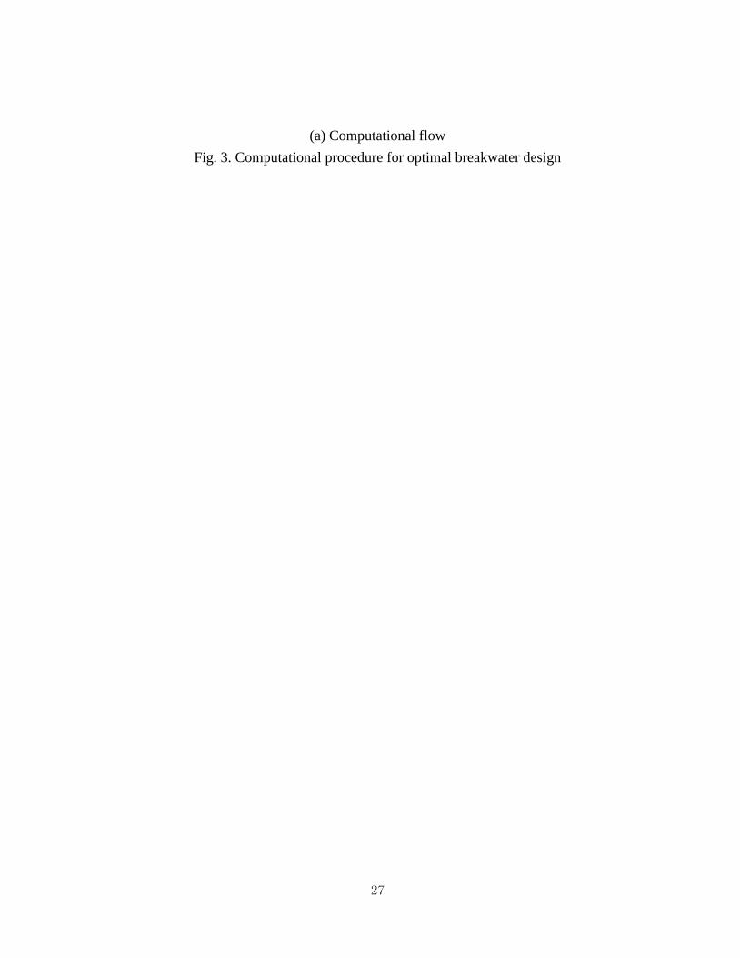
27

(a) Computational flow

Fig. 3. Computational procedure for optimal breakwater design

28

(b) Subroutine A

Fig. 3 (Continued)

Generation of daily maximum significant wave

at breakwater site from Gumbel distribution

Random selection of daily maximum significant wave

from normal distribution

Wave transmission

by Goda-Heijn model

Calculated transmitted wave height

> 0.5 m

Count days of stoppage of harbor operation

Evaluation of damage cost by wave overtopping

No

Yes

Repeat fo

r 365 d

ays

29

(c) Subroutine B

Fig. 3 (Continued)

Generation of yearly maximum deepwater wave

Estimation of significant wave at breakwater site

Generation of individual waves

for storm duration

Computation of wave force

by individual wave

with stochastic variations

Estimation of sliding distance

by individual wave

Calculation of total sliding distance in annual storm event

Sliding distance is

accumulated for i Sum of iT

30

100 1000 10000

Number of simulations

0

2E+006

4E+006

6E+006

8E+006

1E+007

Da

ma

ge

co

st

($)

average

standard deviation

maximum

minimum

(a)

100 1000 10000

Number of simulations

0

2E+006

4E+006

6E+006

8E+006

1E+007

Da

ma

ge

co

st

($)

average

standard deviation

maximum

minimum

(b)

Fig. 4. Calculated economic damage cost versus number of simulations: (a) Latin

hypercube sampling, (b) Conventional random sampling

31

10 20 30 40 50 60 70 80 90 100

Return Period (year)

1E+008

1.2E+008

1.4E+008

1.6E+008

1.8E+008

Ex

pe

cte

d T

ota

l L

ifeti

me C

os

t ($

)

0

0.4

0.8

1.2

1.6

2

Ex

pe

cte

d S

lid

ing

Dis

tan

ce

(m

)

Exp. Cost (w/o discount rate)

Exp. Cost (with discount rate)

Exp. Sliding distance

Toler. Sliding distance

Tolerable Sliding Dist. = 0.3 m


Fig. 5. Curves of expected sliding distance and expected total lifetime costs computed by

including only initial construction cost and rehabilitation cost with and without

consideration of discount rate in water depth of 19 m

32

10 20 30 40 50 60 70 80 90 100


1E+008

2E+008

3E+008

4E+008

5E+008

Ex

pe

cte

d T

ota

l L

ifeti

me C

os

t ($

)

0

0.4

0.8

1.2

1.6

2

Ex

pe

cte

d S

lid

ing

Dis

tan

ce

(m

)

Exp. Cost (Rehabilitation only)

Exp. Cost (Rehabilitation + Operation stoppage)

Exp. Cost (Rehabilitation + Operation stoppage + Harbor shutdown)

Exp. Sliding distance

Toler. Sliding distance



Fig. 6. Curves of expected total lifetime costs for showing the effects of economic

damage costs due to temporal stoppage of harbor operation and long-term harbor

shutdown in water depth of 19 m

33

10 20 30 40 50 60 70 80 90 100


1E+008

1.2E+008

1.4E+008

1.6E+008

Ex

pe

cte

d T

ota

l L

ifeti

me C

os

t ($

)

0

0.4

0.8

1.2

1.6

2

Ex

pe

cte

d S

lid

ing

Dis

tan

ce

(m

)

Exp. Total Cost

Exp. Sliding Distance

Toler. Sliding Distance



Fig. 7. Curves of expected sliding distance and expected total lifetime cost in water depth

of 14 m

34

10 20 30 40 50 60 70 80 90 100


1.2E+008

1.6E+008

2E+008

2.4E+008

2.8E+008

Ex

pe

cte

d T

ota

l L

ife

tim

e C

os

t ($

)

0

0.4

0.8

1.2

1.6

2

Ex

pe

cte

d S

lid

ing

Dis

tan

ce

(m

)

Exp. Total Cost





Fig. 8. Curves of expected sliding distance and expected total lifetime cost in water depth

of 24 m

35

10 20 30 40 50 60


1E+008

2E+008

3E+008

4E+008

Ex

pe

cte

d T

ota

l L

ifeti

me C

os

t ($

)

0

0.4

0.8

1.2

1.6

2

Exp

ecte

d S

lid

ing

Dis

tan

ce (

m)

Exp. Total Cost



4%

6%

8%

10%



Fig. 9. Expected total lifetime costs calculated with different discount rates in water

depth of 19 m

36

10 20 30 40 50 60 70 80 90 100


8E+007

1E+008

1.2E+008

1.4E+008

1.6E+008

1.8E+008

2E+008

Ex

pe

cte

d T

ota

l L

ife

tim

e C

os

t ($

)

0

0.4

0.8

1.2

1.6

2

Ex

pe

cte

d S

lid

ing

Dis

tan

ce

(m

)

Exp. Total Cost





0.05 SMAX

0.1 SMAX

0.2 SMAX

0.5 SMAX

Fig. 10. Expected total lifetime costs calculated with different criteria of caisson sliding

distance for harbor shutdown in water depth of 14 m

37

10 20 30 40 50 60 70 80 90 100


8E+007

1E+008

1.2E+008

1.4E+008

1.6E+008

1.8E+008

2E+008

Ex

pe

cte

d T

ota

l L

ife

tim

e C

os

t ($

)

0

0.4

0.8

1.2

1.6

Exp

ecte

d S

lid

ing

Dis

tan

ce (

m)

Exp. Total Cost





0.05 SMAX

0.1 SMAX

0.2 SMAX

0.5 SMAX



38

10 20 30 40 50 60 70 80 90 100


1E+008

1.5E+008

2E+008

2.5E+008

3E+008

3.5E+008

Ex

pe

cte

d T

ota

l L

ife

tim

e C

os

t ($

)

0

0.4

0.8

1.2

1.6

2

Ex

pe

cte

d S

lid

ing

Dis

tan

ce

(m

)

Exp. Total Cost





0.05 SMAX

0.1 SMAX

0.2 SMAX

0.5 SMAX



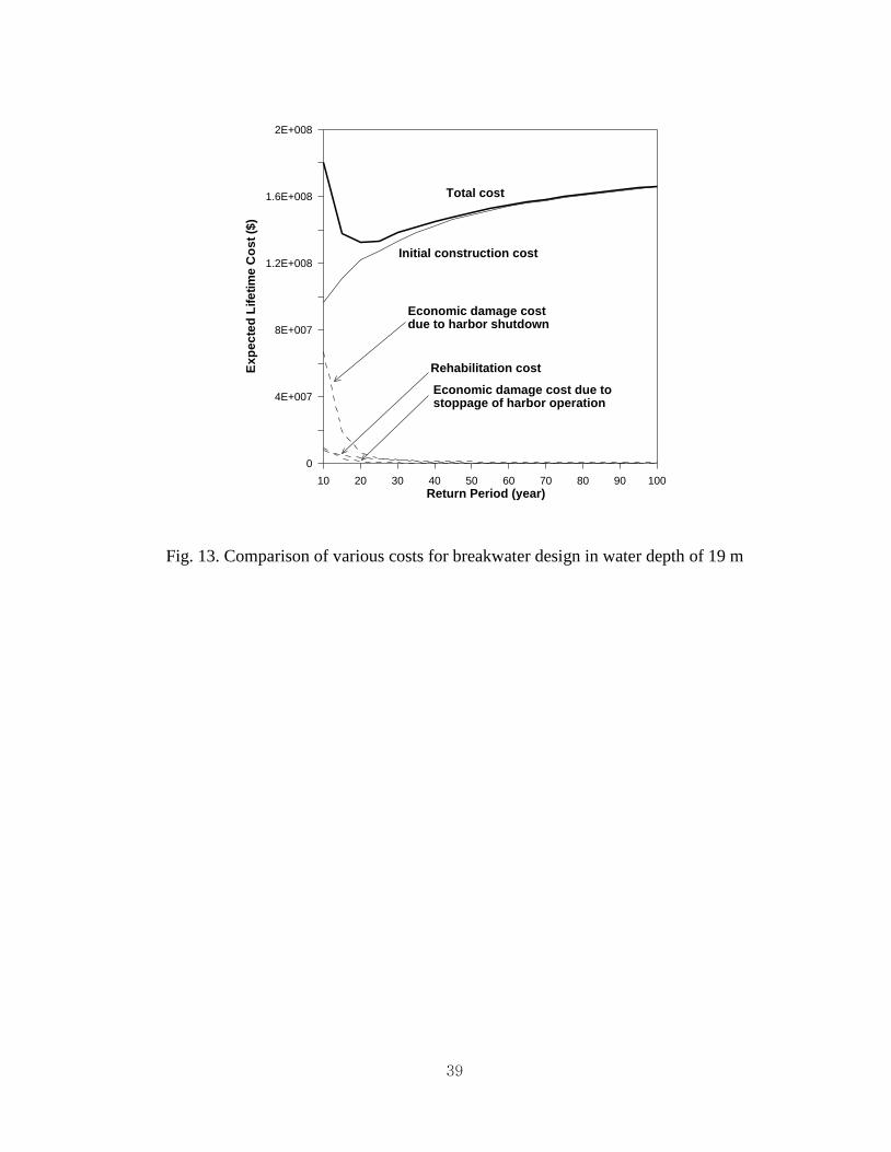
39

10 20 30 40 50 60 70 80 90 100


0

4E+007

8E+007

1.2E+008

1.6E+008

2E+008

Ex

pe

cte

d L

ife

tim

e C

os

t ($

)

Total cost

Initial construction cost

Economic damage cost due to harbor shutdown

Rehabilitation cost

Economic damage cost due tostoppage of harbor operation

Fig. 13. Comparison of various costs for breakwater design in water depth of 19 m

Documents

Effects of Discount Rate and Various Costs on Optimal ...s-space.snu.ac.kr/bitstream/10371/67633/3/Paper-D-09-00052.pdf · 2 distance, expected total lifetime cost, optimal design