Embed Size (px)
Citation preview

Effects of Channel Power on Trade Promotion Budget and Allocation: A Market Experimental Analysis
Hong Yuan, Miguel I. Gómez and Vithala R. Rao*
April 2009
*Hong Yuan is Assistant Professor, Department of Business Administration University of Illinois ([email protected]); Miguel I. Gómez is Assistant Professor, Department of Applied Economics and Management, Cornell University ([email protected]); and Vithala R. Rao is Deane W. Malott Professor of Management and Professor of Marketing and Quantitative Methods, Johnson Graduate School of Management, Cornell University ([email protected]).

1
Effects of Channel Power on Trade Promotion Budget and Allocation: A Market Experimental Analysis
Abstract
We design a market experiment to examine the impact of channel power on trade promotion
budget and its allocation. Our experimental results show that a manufacturer with higher channel
power offers a smaller percentage trade promotion budget and decreases allocation to discount-
based promotions such as off-invoices. Conversely, a retailer with higher channel power tends to
receive larger trade promotion budgets and to increase allocation to discount-based promotions.
We validate these findings with econometric analysis of industry data. Overall, results suggest
that market experiments can shed light on complex negotiations in the distribution channel for
which industry data are often hard to obtain. We discuss implications of our results for managers
and policy makers.

2
Introduction
Trade promotions comprise a growing category of manufacturer incentives directed to
retailers rather than to end consumers. These promotions are designed to influence resellers’
sales and prices by providing various inducements. Manufacturers of consumer-packaged goods
(CPGs) are increasing their trade promotions worldwide. For example, in the US, CPG
manufacturers have increased their trade promotions to retailers eight-fold since 1996, totaling
80 billion dollars in 2004 (Joyce 2005). Trade promotion spending of U.S. manufacturers
accounted for an unprecedented 53 percent of their average marketing budget in 2006 (versus 25
percent two decades ago) and was their second largest expense after the cost of goods
(Cannondale 2007). In Europe, trade promotion budgets were over 14 percent of CPG
manufacturers’ gross sales in 2003 and the largest fifty firms allocated about €100 billion on
trade promotions that year (Lawrie 2004). Moreover, Challier (2008) estimates that trade
promotion expenditures represent about 20% of the total profit-and-loss in UK CPG industry.
Trade promotions are also growing in emerging economies, hand in hand with the globalization
of supply chains (Reardon, Henson and Berdague, 2007).
In spite of their growth, trade promotion negotiations often generate conflict in the
distribution channel, particularly regarding two major decisions: the budget and its allocation.
Trade promotion budgets impact directly the effective wholesale price paid by retailers and profit
sharing among members of the distribution channel. Moreover, manufacturers and retailers
decide on the budget allocation between two broad promotion types: discount- and performance-
based. A manufacturer may offer a retailer discount-based trade promotions, in which a per-case
discount is given for all retailer purchases of a given brand during a limited period of time (e.g.
off-invoices). Or, a manufacturer may negotiate with a retailer performance-based trade
3
promotions, in which a discount per case is given after a pre-specified level of retail sales
performance (e.g. target sales volume per week) has been completed and verified by retail sales
scanning data (e.g. scan-backs).
The economic and marketing literatures have addressed the impact of channel power on
trade promotions. 1 A strain of research primarily from industrial organization economics
suggests that channel structure influences the negotiation of trade promotions (Cotterill 2001;
Patterson and Richards 2000; Sullivan 2002; Scheffman 2002; Young and Hobbs 2002;
Hamilton 2003). Likewise, marketing researchers develop conceptual methods to understand the
links between channel power and trade promotion outcomes (Ailawadi, Farris, and Shames 1999;
Kasulis et al. 1999) and use industry data to examine the impact of manufacturer/retailer
characteristics on trade promotion decisions (e.g., Gómez, Maratou, and Just 2006; Gómez, Rao,
and McLaughlin 2007). This empirical evidence have been formalized using analytical models
based on game theory to study the impact of market structure on trade promotion outcomes and
on channel member welfare (Cui, Raju, and Zhang 2008; Drèze and Bell 2003; Bruce, Desai, and
Staelin 2005).
A common problem encountered in the literature is the difficulty in obtaining data on
trade promotions because they are part of a firm’s marketing expenditures (Skibo 2007; Drèze
and Bell 2003; Kasulis et al. 1999). Consequently, in this study we design a market experiment
that allows us to examine the impact of channel power on trade promotion decisions (budget and
its allocation) and the resulting channel profits. We employ a conceptual model of channel power
rooted in the distribution channel literature (Coughlan et al. 2006; Rangan 2006) and develop
1 Here we use “channel power” instead of “market power”. “Channel power” in marketing is used somewhat liberally and it is defined as the ability of a channel member to control the marketing strategy of another member at a different level of distribution (El-Ansary and Stern 1972). This definition is obviously different from the definition of market power in economics: that is, the ability to increase prices away from competitive levels.
4
testable hypotheses. In our controlled experiments, we manipulate the degree of channel power
(strong or weak) and the nature of relationship between manufacturer and retailer (symmetric or
asymmetric) and collect extensive data to test our hypotheses. In addition, we validate our
findings in the market experiment using industry data from a food retailing survey on trade
promotions negotiated with their suppliers.
Our results suggest that (1) a manufacturer with higher channel power offers a smaller
trade promotion budget (as percentage of wholesale price) ; (2) allocation to discount-based
(performance-based) trade promotions decreases (increases) with manufacturer channel power
and increases (decreases) with retailer channel power; (3) retailer margins are higher when the
trade promotion budget is allocated to discount-based types; and (4) trade promotion decisions
affect profit sharing between the manufacturer and the retailer within the channel but have little
impact on total channel profits.
The rest of this paper is organized as follows. We first describe our focal trade promotion
decisions, our conceptual model and state our hypotheses. Next, we describe the experimental
design and analysis, and discuss the findings from market experiments. Subsequently, we assess
the validity of our experimental findings using industry data. The last section concludes,
discusses managerial and policy implications, and proposes topics for future research.
Trade Promotion Decisions
We focus on trade promotion budget and its allocation between off-invoices (discount-
based) and scan-backs (performance-based). There are two likely scenarios of trade promotion
decisions. One is that budget and allocation follow a two-step process in which a manufacturer
first observes the channel power structure and decides on its trade promotion budget.

5
Subsequently, manufacturer and retailer decide the allocation between off-invoices and scan-
backs. The second scenario is that budget and allocation are simultaneously determined during
negotiations between the manufacturer and the retailer in the dyad.
To better understand the framework in which trade promotion negotiations occur, we
interviewed a convenience sample of retail buyers from fifteen supermarket companies to
determine which of the above sequences was more appropriate to describe trade promotion
negotiations. According to these respondents, budget and allocation decisions are in general not
simultaneously determined. Our respondents reported that in 70 percent of the cases, the
manufacturer determines an annual promotion budget for each retail brand account (generally as
some function of last year's sales and sales projections for the coming year). Once the
manufacturer has determined the budget, the retailer and the manufacturer decide how
promotional funds can best be allocated, depending on the channel power structure. However,
the respondents in this survey also pointed out that in a few cases, the retailer is successful in
continuing to extract additional promotional funds from the supplier as the year progresses, after
the initial budget determination.
Gomez, Rao and McLaughlin (2007) statistically test alternative scenarios of trade
promotion decisions and find no significant differences between the two specifications described
above. The authors select a joint model specification in which the trade promotion budget and its
allocation are jointly determined. The main reason for their choosing a joint model specification
is that their econometric analysis is cross sectional from a sample of retailers with little
information about the decision process. In contrast, in the market experiment we follow the
predominant process as per our interviews with retailers and assume that a manufacturer
6
observes the channel power structure and selects the budget. Subsequently, either the
manufacturer or the retailer selects the allocation of the budget.
Conceptual Model
In Figure 1, we present our conceptual framework for the market experiment, specifying
our strategy to manipulate channel power and its consequences for trade promotion budget and
allocation decisions. This framework is based on distribution channel theories proposed by
Coughlan et al. (2006) and Rangan (2006). Consequently, we define channel power as “the
ability of one channel member (A) to get another channel member (B) to do something it
otherwise would not have done” (Coughlan et al. 2006, p. 197). Similarly, Rangan (2006)
discuses channel power in terms of the ability of one channel member to influence the decisions
on other(s) channel member(s). Our focus is on the impact of channel power on trade promotion
decisions and resulting profits.
[Insert Figure 1 here]
We focus on two important dimensions of channel power: the channel structure and the
ability of channel members to influence trade promotion allocation decisions.2 We consider two
aspects related to channel structure: channel member market share and the channel member
ability to sell to (or buy from) alternative sources outside the dyad (Rangan 2006). Channel
member market share is one of the most important variables that firms employ to influence the
marketing strategies of other channel members (Rangan 2006). A manufacturer with higher
channel power can seek alternative selling channels while a retailer with higher channel power
2 Our experimental design would become too complex if we include all sources of channel power discussed in the literature. Therefore, we abstract from the brand and other sources of channel power include power associated with having a unique brand and legal or institutional power through legal protections such as patents, trademarks, trading norms and informal business practices (Rangan 2006).

7
can seek alternative sources of supply. This dimension of channel power can be traced back to
the notion of power as a function of dependence (Emerson 1962 and El-Ansary and Stern’s
(1972)). By reducing dependence on a specific channel member through outside options, a firm
increases its own channel power. Therefore in our market experiment we define a “strong”
manufacturer (retailer) as a manufacturer (retailer) with a large market share and with ability to
sell to (buy from) retailers (manufacturers) outside the dyad. Conversely, a “weak”
manufacturer (retailer) has a small market share and cannot sell (buy) outside the dyad.
Therefore, the trade promotion decisions in a given dyad may involve symmetric (strong
manufacturer – strong retailer; or weak manufacturer – weak retailer) and asymmetric (strong
manufacturer – weak retailer; or weak manufacturer – strong retailer) channel structures.
The second source of channel power in our conceptual model is the ability to influence
the trade promotion allocation decisions between off-invoices and scan-backs. This aspect has
been often referred to as bargaining power in the literature. For example, manufacturers may
have the ability to influence the allocation decision because they have channel power associated
with having a unique brand (Coughlan et al. 2006; Gómez, Maratou, and Just 2007; Rangan
2006). Likewise, retailers may be able to influence the allocation decision because they may
have access to hard-to-reach customers and market intelligence (Rangan 2006). The empirical
literature shows that channel members with ability to select the trade promotion type can
influence the distribution of profits along the supply chain (Drèze and Bell 2003; Gómez,
Maratou, and Just 2007, Cotterill 2001). Therefore in our market experiment we define a
“dominant” manufacturer (retailer) as a manufacturer (retailer) that has the ability to make the
allocation decision. In contrast, a “non-dominant” manufacturer (retailer) does not have the
ability to influence the allocation decision.

8
Hypotheses
Channel structure and trade promotion budget: The most studied question in industrial
organization economics examines how market structure affects prices (Bresnahan 1989). A
stream of research primarily from industrial organization economics examines the causes and
consequences of trade promotions in the context of relative channel power in the distribution
channel (Cotterill 2001; Patterson and Richards 2000; Sullivan 2002; Scheffman 2002; Young
and Hobbs 2002; Hamilton 2003). This literature shows that trade promotions may produce
demand distortions and may move prices away from the equilibrium.
The marketing literature offers evidence of the links between channel power and trade
promotion budget. Mela, Gupta and Jedidi (1998) show that the dramatic shift of marketing
expenditures from direct consumer advertising to trade promotions have increased the channel
power of retailers. More recently, Cui, Raju and Zhang (2008) develop a game theoretical model
to show that manufactures have incentives to price discriminate between dominant retailers and
smaller retailers lacking channel power. The authors show that it is optimal for manufacturers to
offer the same list price to all retailers, but they can implement price discrimination through trade
promotions.
Since trade promotion budgets affect the effective wholesale price, industrial
organization theory implies that manufacturers with greater channel power should allocate
smaller trade promotion budgets. Likewise, retailers with strong channel power receive greater
trade promotion budgets because they have the leverage to command a higher percentage and
lowering the effective price paid to manufacturers. Therefore, we offer the following hypothesis:

9
H1: Trade promotion budget measured as a percentage of wholesale price of a strong manufacturer (retailer) is smaller (larger) than the trade promotion budget of a weak manufacturer (retailer).
Ability to influence the allocation decision and allocation to off-invoices and scan-backs:
The economics and marketing literatures have addressed the allocation between performance-
and discount-based trade promotions in the context of channel power. Ailawadi, Farris and
Shames (1999) demonstrate that performance-based trade promotions linking manufacturer and
retail prices, such as scan-backs, may enhance the ability of manufacturers to coordinate
distribution channels. This is contrary to off-invoice allowances, which enable resellers to
engage in forward buying or partial pass-through. Drèze and Bell (2003) employ economic
theory to formalize findings in Ailawadi, Farris and Shames (1999) and show that manufacturers
can design scan-back trade promotions that provide the same benefits to the retailer as off-
invoice promotions. More recently, Kurata and Yue (2008) develop a model focusing on scan-
backs, which are a particular form of performance-based trade promotions. The authors show
that manufacturers and other members of the supply chain always benefit from scan-backs. In
contrast, retailers benefit from scan-backs only when they are offered together with buy-backs, in
which the manufacturer agrees to buy back some or all of the products that are not profitable to
the retailer.
Empirical evidence supports the implications of the models developed by Drèze and Bell
(2003) and Kurata and Yue (2008). Gómez, Maratou and Just (2006) use supermarket data to
show that retailer bargaining power increases the allocation of funds to off-invoice trade
promotions through higher share of private label and retailer size, while manufacturer bargaining
power decreases the allocation of funds to off-invoice trade promotions by establishing formal
policies of negotiation. Finally, Gómez, Rao and McLaughlin (2007) find that manufacturer

10
variables such as brand price premium as well as annual retailer sales determine trade promotion
budgets. In addition, the authors show that retail companies with larger annual sales, stronger
brand positioning, and formal policies are able to increase the allocation to off-invoices and to
decrease allocation to performance-based trade promotions.
These results imply that a dominant manufacturer would prefer scan-back over off-
invoices and conversely, a dominant retailer would choose off-invoices over scan-backs.
Therefore, we offer the following hypothesis:
H2: The allocation to off-invoices (scan-backs) increases (decreases) with retailer’s ability to influence the allocation decision and decreases (increases) with manufacturer’s ability to influence the allocation decision.
Channel structure and allocation to off-invoices and scan-backs: The trade promotion
literature suggests that scan-backs allow manufacturers to coordinate the distribution channel,
ensuring that trade promotions are reflected in lower retail prices (Ailawadi, Farris, and Shames
1999). Theoretical and empirical work by Bell and Drèze (2002) and Drèze and Bell (2003)
compare retailer pricing and profitability between off-invoices and scan-backs. Their theory
shows that, ceteris paribus, retailers prefer off-invoices over scan-backs while manufacturers
prefer scan-backs over off-invoices. Retailers prefer off-invoices because of the flexibility
offered in their use (e.g., allowing the retailer to forward buy, and even engaging in diverting)
and the possibility of not having to pass-through all discounts to the consumer. However, this
greater retailer flexibility comes at a cost to the manufacturers: they lose control over their
marketing mix. Kasulis et al. (1999) argue that a manufacturer with a strong position in terms of
channel structure should maximize allocation to performance-based trade promotions. In
addition, Gómez, Maratou and Just (2007) provide empirical evidence that larger manufacturers
11
can influence the allocation in favor to performance-based types while larger retailers can
increase allocation to off-invoices. Therefore, we posit the following hypothesis:
H3: A strong manufacturer (retailer) decreases the allocation to off-invoices (scan-backs).
Market Experiment
We utilize a series of market experiments to simulate markets via networked computers
and observe how manufacturers and retailers behave in an interactive setting. In the experiments,
manufacturers earn experimental dollars (EDs) by selling to the retailers while retailers earn EDs
by purchasing from manufacturers and selling to the consumers. Manufacturers and retailers
make decisions to maximize their ED earnings.
In our experiment we manipulate channel power following the conceptual framework
explained in Figure 1. A manufacturer with “strong” channel power produces more units (i.e.,
commands a larger market size) than its “weak” counterpart and also has the ability to sell excess
production outside the dyad in an external market. Similarly, a retailer with strong market power
enjoys a larger potential consumer demand than a weak retailer and has the ability to procure
units outside the dyad when consumer demand exceeds the quantity ordered from the
manufacturer in the dyad. A “weak” manufacturer (retailer) cannot sell (buy) outside the dyad.
We also manipulate the ability to influence the trade promotion allocation decision: The
“dominant” party within the dyad, which is randomly assigned by the computer as the
manufacturer or the retailer, decides whether the entire trade promotion budget is allocated to
off-invoice or scan-back.
To test the above hypotheses, we use a 2 (Symmetric versus Asymmetric Market
Structure – between subjects) X 2 (Manufacturer Dominant versus Retailer Dominant – within
subject) X 3 (replications) design. A “symmetric” channel structure includes conditions where
12
retailer and manufacturer are both strong or both weak whereas an “asymmetric” channel
structure includes conditions where the manufacturer is “strong” and the retailer is “weak” or
vice-versa. In all conditions, manufacturers make the trade promotion budget decisions. In Table
1 we show the experimental conditions. Note that for asymmetric markets we only focus on the
conditions where the stronger firm is the dominant player.
[Insert Table 1 here]
We ran this experiment in eight sessions with four symmetric and four asymmetric
experimental markets. For each session, we recruited twenty students. In all, one hundred and
twenty undergraduate students and forty MBA students participated in the study. At the
beginning of each session, ten subjects were randomly assigned as manufacturers and ten as
retailers and they remained in the same roles throughout the experiment. In about 90 minutes, the
subjects traded as manufacturer-retailer dyads using experimental dollars (EDs) in a series of
market periods.
The experiment was programmed using Z-tree3 and all the transactions were completed
through networked computers. In each period, the computer system first randomly selects a
manufacturer (M) and a retailer (R) to form a dyad. In symmetric (asymmetric) markets, 5 of the
10 dyads have strong manufacturers selling to strong (weak) retailers and the other 5 dyads have
weak manufacturers selling to weak (strong) retailers. Then five markets were randomly formed,
each having two different types of manufacturer-retailer dyads. In other words, each market in
the symmetric condition consists of a M(strong)-R(strong) pair and a M(weak)-R(weak) pair
whereas each market in the asymmetric condition consists of a M(strong)-R(weak) pair and a
M(weak)-R(strong) pair. Since there were 5 markets in a given period, the subjects did not know
in advance which markets they belonged to and who they were playing with. 3 Zurich Toolbox for Readymade Economic Experiments (Fischbacher 2007)

13
For each market, the computers simulate 100 robot consumers, each demanding one unit
of a hypothetical product. Each robot consumer has a value for the product which represents the
highest price this consumer is willing to pay. The value for any consumer is a random draw from
a uniform distribution between 0 and 10 EDs. The strong manufacturer (retailer) in the market
produces (has the potential to sell) 80 units whereas the weak manufacturer (retailer) produces
(has the potential to sell) only 20 units.
At the beginning of the experiment, instructions were read and questions were answered
publicly, followed by a practice period to familiarize subjects with the experimental
environment. During the practice period, the experimenter explained information on each screen
and answered questions as the practice experiment progressed.
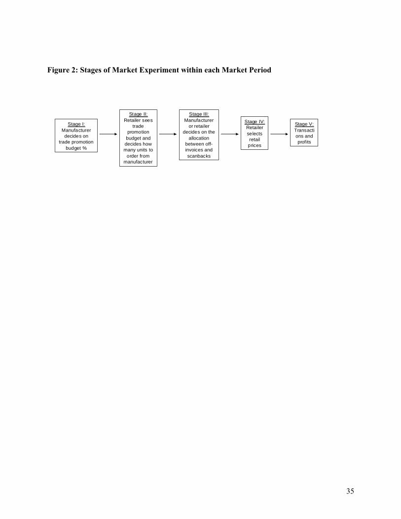
Within each market period there are five stages (Figure 2). In the first stage, given
wholesale price PM = 2 EDs and the information about manufacturer and retailer power within
the dyad, the manufacturer decides on the trade promotion budget (TP %) as a percentage
discount of PM. In the second stage, retailers decide the number of units to order from the
manufacturer (QM) knowing the trade promotion budget offered by the manufacturer (TP %). In
the third stage, the dominant firm (manufacturer or retailer) within a dyad makes the allocation
decision between off-invoices and scan-backs. If the trade promotion budget is allocated to off-
invoices, the units used to determine the total amount of trade promotion (QTP) will be the same
as the quantity ordered by the retailer (QM). However, if the trade promotion budget is allocated
to scan-backs, then the units considered in trade promotion (QTP) is equal to the quantity sold by
retailer to the end consumer (QR). Thus, the total amount of trade promotion paid to the retailer
Boff-invoices = TP% * PM * QM (and Bscanbacks = 0) if off-invoices are selected. If scan-backs are
chosen, then the trade promotion allowance Bscanbakcs = TP% * PM * QR (and Boff-invoices = 0). In

14
the fourth stage, given the trade promotion allowance and type selected by the dominant firm,
retailers make decisions on the retailer price (PR) as a value between 0 and the maximum
consumer value 10EDs. In the fifth stage, transactions were completed by computer-simulated
robot buyers. If a consumer’s value is higher than or equal to the retail price, he/she will
purchase one unit of the product from the retailer. Otherwise, the consumer will not purchase.
For the unsold units (QM - QR), there is a per inventory cost of I = 0.10EDs for the retailer.
[Insert Figure 2 here]
To enable learning, subjects were informed of the transaction outcomes (including units
sold, inventory left, the amount and type of trade promotion and profits) in the current period
before they moved on to the next period. Manufacturer profits depend on (1) revenue; (2) trade
promotion budget and its allocation; and (3) its ability to sell excess production elsewhere. A
weak manufacturer cannot sell its excess production outside the dyad whereas a strong
manufacturer sells its excess production elsewhere with a profit margin that is 50% of the profit
margin it gets by selling the product to the retailer in the dyad4. Therefore, profits for weak
manufacturers (ΠW,M) were calculated as:
(1) )**%()*(, MTPMMMW PQTPPQΠ −= ,
where the first term in parenthesis is manufacturer revenues and the second is trade promotion
budget. Likewise, the profits for strong manufacturers (ΠS,M) are:
(2) ]*5.0*))80[()**%()*(, MMMTPMMMS PQPQTPPQΠ −+−= ,
4 In order for the subjects to focus on within-dyad trade promotion decisions, we made sure that profit margin outside the dyad was lower (50% here) than the profit margin within the dyad.

15
where the first two terms are the same as in equation (1) and the third term in parenthesis
represents manufacturer profits accruing to units sold outside the dyad.
Retailer profits depend on (1) revenue; (2) trade promotion budget and its allocation; (3)
inventory costs for unsold units; and (4) its ability to procure shortages from elsewhere.
A weak retailer cannot procure units from elsewhere outside the dyad. Therefore, the quantity
sold to consumers (QR) cannot exceed the quantity ordered from the manufacturer (QM). If
consumer demand exceeds the units ordered from the manufacturer in the dyad (QR > QM), a
strong retailer procures the shortage (Qoutside) from elsewhere with a profit margin that is 50% of
the profit margin it gets by selling the units ordered from the manufacturer in the dyad.
Therefore, profits for weak retailers (ΠW,R) are:
(3) ]*)[()**%()*()*(, IQQPQTPPQPQΠ RMMTPMMRRRW −++−= ,
where the first term is retailer revenues; the second term is the cost of goods sold; the third term
is the trade promotion income; and the fourth term is the inventory cost corresponding to unsold
units (when QM>QR). The profit for a strong retailer (ΠS,R) yields:
(4) ]*5.0*)[(
]*)[()**%()*()*(,
outsideMR
RMMTPMMRRRS
QPPIQQPQTPPQPQΠ
−+−++−=
.
In equation (4), the first four expressions in brackets are the same as in equation (3) and
the fifth term represents the profits accrued to units procured outside the dyad. Total profits were

16
accumulated throughout the periods and then converted into real dollars. Each subject was paid
$5-$10 privately at the end of the experiment, depending on performance.
Statistical Procedures and Operationalization of Variables
On average, subjects played thirty six periods in each ninety-minute session. We analyze
data from the last fifteen periods of the session to allow learning. Our unit of observation is the
manufacturer-retailer dyad. We develop three measures of channel power. The first is a vector of
dummy variables (strong-strong, weak-strong, strong-weak, weak-weak) reflecting the type of
dyad (e.g. strong-strong equals 1 if both manufacturer and retailer are strong; zero otherwise). In
addition, we create a variable that measures exercised channel power. The exercised channel
power of manufacturer i is defined as
(5) MC_POWERi,t = M_PROFIT i,t / Manufacturer Maximum Possible Profit i,t, where t is period. Therefore, MC_POWERi,t ranges from zero to one with larger values indicating
greater channel power of manufacturer i. In the same spirit, the exercised channel power of
retailer j is defined as:
(6) RC_POWERj,t = Actual Retailer Profitj,t / Retailer Maximum Possible Profitj,t.
We combine the exercised channel power into a single measure of relative channel power
(RELC_POWER) as the ratio of the manufacturer i and retailer j indices:
(7) RELC_POWERi,j,t = MC_POWERi,t / RC_POWERj,t.

17
In our experiment, bargaining power or dominance is accounted for by the ability of
manufacturers and retailers to select the trade promotion types. Therefore we define a dummy
variable (M_DOMINANTi,t) equal to one if the manufacturer i makes the allocation decision in
the dyad; zero otherwise.
The dependent variables are: (i) the trade promotion budget offered by manufacturer i to
retailer j in period t (TP_BUDGETi,j,t), expressed as a percent of experimental dollars allocated to
the wholesale price; (ii) a dummy variable for allocation type (OFFINVOICESi,j,t), which equals
one if the budget offered by manufacturer i to retailer j in period t is allocated to off-invoices and
zero otherwise and (iii) the retail margin (R_MARGINj,t) which equals to retail prices chosen by
the retailer j in period t minus the wholesale price in period t. Z is a vector of variables
controlled in the experimental design (symmetric versus asymmetric experimental conditions and
types of dyads).
The models to test Hypotheses 1-3are the following:
H1: Market Power and Trade Promotion Budget
TP_BUDGETi,j,t = F1 ( RELC_POWER i,t,j , Z )
H2: Bargaining Power and Trade Promotion Allocation
OFFINVOICESi,j,t = F2 ( M_DOMINANTi,t , Z)
H3: Market Power and Trade Promotion Allocation
OFFINVOICESi,j,t = F3 ( M_DOMINANTi,t , RELC_POWERi,j,t , Z )
TP_BUDGETi,j,t varies from 0 to 1 given our data collection procedure. Therefore, to test
H1, we employ maximum-likelihood estimation methods using the logistic distribution as the
link function, namely fractional logit (Papke and Wooldridge, 1996). This approach employs
Generalized Linear Models with the Bernoulli log-likelihood function defined as

18
(8) li(b) = yi log [ G(xib) ] + (1-yi) log [ 1 - G(xib) ],
where G(.) is the logistic function G(xib) = 1/[1+exp(-xib)], yi is the fractional variable, xi is a
vector of exogenous variables, and b is the vector of parameters to be estimated. For H2 and H3,
we employ a standard Logit model because the dependent variable OFFINVOICESi,j,t is
dichotomous.
We conduct additional exploratory analysis on our experimental data, using Ordinary Least
Squares, regarding the links between trade promotion decisions and other experimental outcome
variables. These include such aspects as how the allocation of trade promotions between off-
invoices and scan-backs relate to the share of profits and how the trade promotion budget affects
manufacturer and retailer profits, among others.
Empirical Results
Our analysis sample comprises 680 observations for undergraduate students and 298 for
MBA students. The mean values of critical variables in the experiment were comparable among
the two groups. The mean percent trade promotion budget was 21.6 and 19.8 percent for
undergraduates and MBAs, respectively; undergraduates selected off-invoices on 43.5 percent of
the times as compared to 46.0 percent for MBAs; and the mean retailer margin was 2.5 and 3.4
EDs for undergraduates and MBAs, respectively. For undergraduates, our measure of
manufacturer relative power ranges between -4.8 and 1.6 and its mean is -0.5.; and the
manufacturer is dominant in 52.1 percent of the cases. Similarly, for MBA subjects, relative
power ranges from -2.9 and 2.9 (its mean is -0.24) and manufacturers were dominant on 49.7
percent of the periods. MBA students had an average work experience of forty three months and
had an average age of thirty.

19
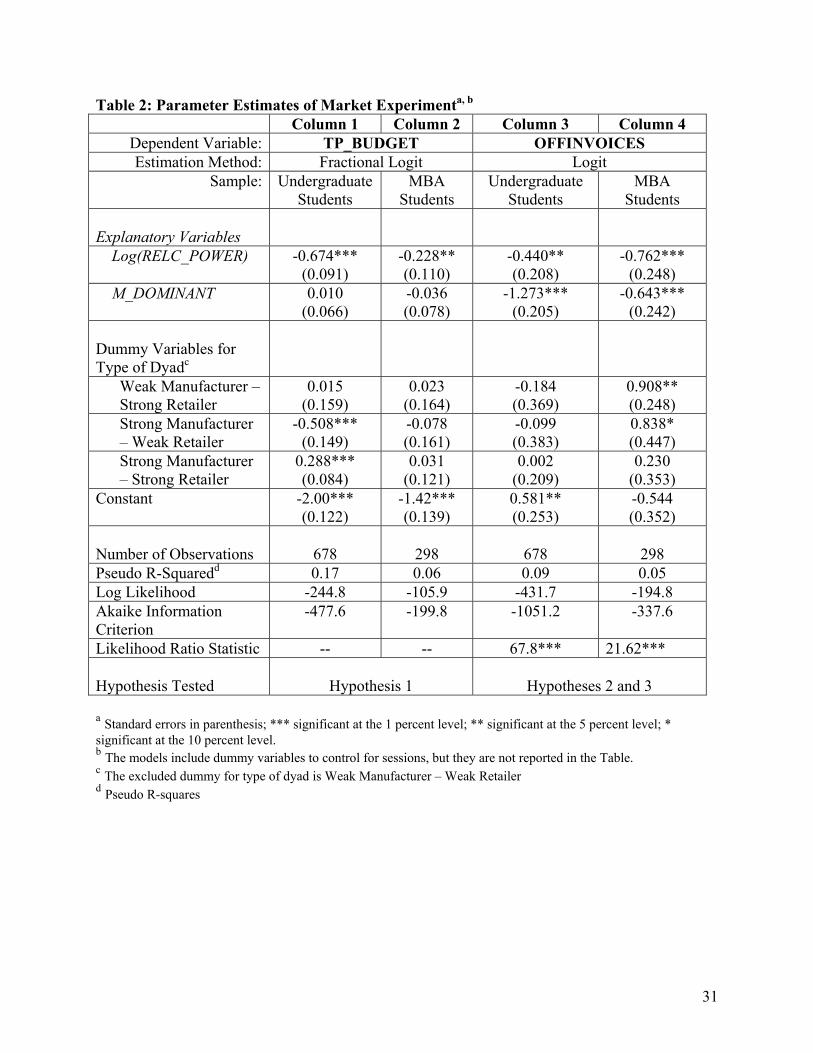
Trade promotion budget - In Table 2 we present results corresponding to each of the
three main hypotheses. Columns 1 and 2 address the impact of manufacturer relative channel
power on trade promotion percent budget in the experiment with undergraduate and MBA
students, respectively. Consider first the experimental results with undergraduate students in
Column 1. Our results provide evidence that a manufacturer with relative channel power
allocates a smaller percentage to trade promotion budgets than manufacturers with less channel
power. The coefficients in Table 2 are obtained from nonlinear models because they do not
represent marginal effects of the focal relationships and they must be computed.5 The marginal
effect indicates that a manufacturer with relative channel power one standard deviation above the
mean has a percent trade promotion budget that is 5.90 percent points smaller than the sample
mean (the standard deviation of the logarithm of RELC_POWER parameter estimate equals
0.65). This result supports hypothesis H1. In addition, the coefficients for dyad-type dummy
variables indicate that, in average, a dyad involving a stronger manufacturer and a weak retailer
has a promotion budget that is 6.8 percent points smaller relative to a weak-manufacturer, weak-
retailer dyad. These results provide additional evidence for hypothesis H1. Interestingly, the
coefficient of M_DOMINANT is statistically insignificant in the trade promotion budget
equation. This suggests that dominance may not affect trade promotion budget, favoring the
argument that manufacturers set the trade promotion first and then negotiate its allocation with
retailers (as stated by a majority of retailers in our preliminary interviews).
5 The partial effect of a given explanatory variable x on E(y / X) is given by xyE ∂∂ /)|( X , or, for specification (3), g(Xβ) βx, where y is the dependent variable, X is the vector of explanatory variables, β is the vector of parameters, βx is the coefficient corresponding to variable x, g(z) ≡ dG(z)/dz = exp(z)/[1+exp(z)]2.

20
The results for the MBA students (who have more work experience) are quite consistent
with those obtained for the undergraduate students (see Column 2 of Table 2).6 The marginal
effect shows that a manufacturer with relative channel power one standard deviation above the
mean has a percent trade promotion budget that is 3.2 percent points smaller than the budget of
the sample mean (the sample standard deviation equals 0.81). The results for the two groups of
subjects together provide substantial support for hypothesis H1.
[Insert Table 2 here]
Allocation of trade promotions - In Column 3, we present maximum likelihood estimates
for the coefficients of the measures of channel power in Equation 2 from data of undergraduate
students to test hypotheses H2 and H3.The Likelihood Ratio (LR) statistic is significant, suggests
that the model explains the variability of the allocation to off-invoices. The coefficient for
M_DOMINANT indicates that when the manufacturer is the dominant player in the channel,
manufacturer tends to select scan-backs relative to off-invoices. In terms of relative probabilities,
the odds ratio of choosing scan-backs is nearly three to one when the manufacturer is dominant
in the dyad. Conversely, dominant retailers tend to prefer off-invoices and reflect these
preferences in their choices. These results provide strong support to H2. The estimated
coefficient of manufacturer relative market power (RELC_POWER) on allocation is positive and
significant at the 5 percent level. This suggests allocation to off-invoices tends to decrease with
relative channel power of the manufacturer. The dummy variables for the type of dyad are all
statistically insignificant. These results provide moderate support to H3.
6 We may add that the results from experiments with undergraduate and MBA subjects are qualitatively similar, even though the estimated magnitudes of the impacts differ somewhat. This is mainly due to the wider range of the percent trade promotion variable for the undergraduate subjects relative to MBA subjects. One possible explanation for this difference is the fact that MBAs have more work experience and familiarity with trade promotion tactics.

21
The replications with MBA subjects provide additional evidence supporting hypothesis
H2 and H3 (see Column 4 of Table 2). That is, a dominant manufacturer is able to allocate a
smaller portion of the budget to off-invoices and a larger portion to scan-backs. More precisely,
the odds ratio of choosing scan-backs is nearly two to one when the manufacturer is dominant in
the dyad, in comparison to the case when the retailer is the dominant party. Our experiments with
MBA subjects also suggest that manufacturers with larger channel power can reduce allocation
to off-invoices. In particular, the marginal effect of log(RELC_POWER) shows that a
manufacturer with relative channel power one standard deviation above the mean has an
allocation to off-invoices that is 15.3 percent points smaller than allocation to off-invoices of the
sample mean (the standard deviation of the logarithm of RELC_POWER parameter estimate
equals 0.81). Further, we assessed the internal validity of our results by predicting the trade
promotion budget and the allocation to off-invoices for the last two periods using estimates
obtained for the first thirteen periods. The root mean square forecast error (RMSE) and the mean
absolute forecast error (MAE) for the trade promotion budget are 0.07 and 0.06 for
undergraduate subjects and 0.09 and 0.08 for MBA subjects. Likewise, for the allocation to off-
invoices equation the model predicted correctly 60 and 65 percent of the time for undergraduate
and MBA subjects, respectively. This indicates a high degree of internal validity for our results.
Additional Analyses - We also investigated the impact of trade promotion negotiations on
other outcome measures (Table 3). For this, we employed single-equation OLS using the White
correction for heteroskedasticity. These results indicate that the subjects in the experiment made
rational decisions, thus providing validity to our findings. For example, our estimates suggest
that manufacturer profits tend to decrease with trade promotion budget; retailer profits tend to
increase with trade promotion budget; but there is no evidence that channel profits depend on the

22
trade promotion budget. Regarding trade promotion allocation (between off-invoices and scan-
backs) and channel profits, we find that manufacturer profits decrease (increase) with off-
invoices (scan-backs) and retailer profits increase (decrease) with off-invoices (scan-backs).
However, we find that the type of trade promotion does not affect channel profits. Therefore, the
net effect of trade promotion budget and its allocation is to transfer profits between the retailer
and the manufacturer. This may explain why it is very hard to employ trade promotions for
channel coordination. We also find that retailer orders and sales tend to increase with trade
promotion budget. This suggests that trade promotions may be an appropriate instrument to keep
or expand market share. Finally, our results indicate that retailer orders increase when expected
trade promotion budget is higher than the actual trade promotion budget offered by the
manufacturer. 7
[Insert Table 3 here]
Further Support Using Industry Data
In this section, we provide additional support to our experimental results using survey
data on trade promotions from 36 supermarket companies. These data are from a survey
conducted by Gómez, Rao and McLaughlin (2007) and supplemented with data from secondary
sources akin to our experimental measures of channel power. This analysis is based on 101
usable observations covering five product categories and over thirty brands. The unit of
observation is a particular brand and not the individual trade promotion contract. The dataset
contains information on the total amount of trade promotion dollars received from manufacturers
and the percent allocation of these funds to off-invoices and to performance-based types. We
7 In the first stage when manufacturers make trade promotion budget decisions, we ask retailers what they expect the trade promotion budget will be.

23
supplemented the survey with secondary data to measure channel structure and ability to select
the trade promotion type, so that these data are comparable to those from the market experiment.
Specifically, to measure channel structure we collected data on brand market share in the
national market (M_SHARE) and data on supermarket market share in the main metropolitan
areas in which they operate (R_SHARE). In turn, we computed the logarithm of the ratio
M_SHARE/R_SHARE to obtain a relative measure of relative market share between a
manufacturer and a retailer in a given dyad (RELATIVE_SHARE). To measure ability to select
the trade promotion type, we employ the following question from the survey: “what percent of
the times do you select the trade promotion type” (R_SELECTS). We estimate the following
equation system:
(9)
,2000 *,
*,,
,2,220*
,2
,1,10,1
=<=≥=
++∂+++=
++∂++=
nforyifyandyifyy
αy
y
ijknnijknijknn
ijkijijk
ijkijijk
εε
εεβ
j23ljkijk
j11ijk
ZλR_SELECTSβHARERELATIVE_S
ZβHARERELATIVE_S
where i, l, j, k represent retailer, manufacturer, product category and brand, respectively. The
endogenous variables are the natural logarithm of trade promotion budget (y1) and its percent
allocation to off-invoices (y*2). The allocation variable is censored at zero and is identified with
an asterisk. The vectors of explanatory variables include the channel power constructs described
above and Zj is vector of other control variables, including product category dummies and price
differences across brands in the same product category (see Gómez, Rao and McLaughlin 2007
for details of estimation procedures).
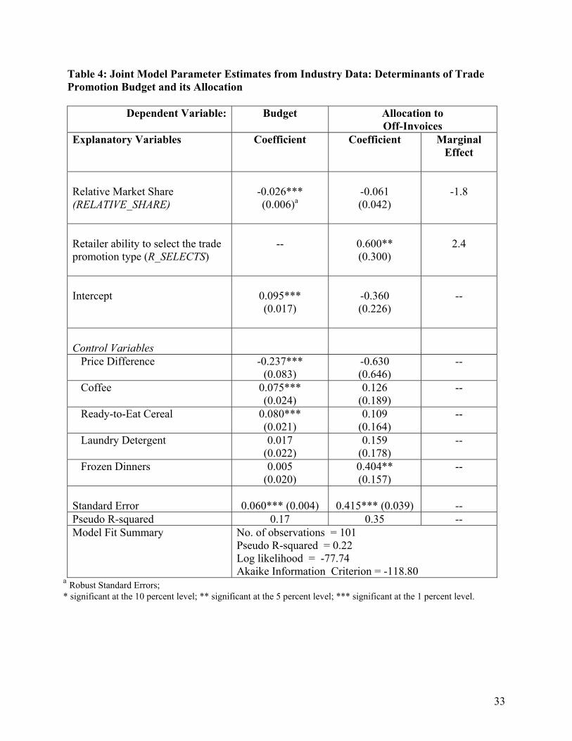
Table 4 shows all parameter estimates and standard errors of the joint model of budget
and allocation to off-invoices. Consider the trade promotion budget equation first. The estimated
coefficient for relative market share (RELATIVE_SHARE) has the expected sign and is

24
significant at 1 percent level. The marginal effect indicate that a manufacturer with a brand
market share relative to the retailer in the dyad 10 percent points above the sample mean has a
percent trade promotion budget 2.6 percent points smaller than the sample mean. This result
provides support for H1 and is consistent with the findings in the experimental design.
[Insert Table 4 here]
Regarding the allocation of trade promotion budget, our results show that increased
retailer ability to select the trade promotion type (R_SELECTS) is positively related to the
allocation of trade promotion budget to off-invoices at the five percent significance level. The
marginal effect indicates that retailers that are able to select the trade promotion type one
standard deviation more often than the sample mean can increase allocation to off-invoices by
2.4 percent (the sample mean and standard deviation of R_SELECTS are 0.5 and 0.16,
respectively). Conversely, manufacturers with increased ability to select the trade promotion type
tend to reduce allocation to off-invoices. This result provides support to H2. The coefficient of
the relative market share of the manufacturer and retailer in a given dyad (RELATIVE_SHARE)
indicates that manufacturer with the a relative market share one standard deviation above the
mean has an allocation to off-invoices that is 1.8 percent points lower than the mean. This
coefficient exhibits the expected negative sign but it is statistically insignificant, thus failing to
provide support for H3.
Conclusions, Limitations and Future Research
In this study, we designed a market experiment to study the influence of two important
dimensions of channel power, market structure and ability to influence the trade promotion type,
on trade promotion decisions made by manufacturers and retailers and their implications for

25
profit sharing among channel members. While empirical research based on data collected in the
field may be limited to certain industries and countries, the experimental approach allows us to
examine the effects of key variables in a context-free environment. Overall, we are able to find
support for our hypotheses and validate our conceptual model with industry data.
Our results indicate that manufacturers with a stronger position in the channel structure
(larger market share and ability to sell outside the dyad) tend to have smaller trade promotion
budgets and to increase allocation to scan-backs. In contrast, retailers with a relative stronger
position in the dyad (larger market share and ability to buy outside the dyad) tend to receive
bigger trade promotion budgets and are able to increase allocation to off-invoices.
The primary contribution of our study is to show that market experiments may be a useful
approach to examine trade promotion decisions in the supply chain, taking into account that
companies are often reluctant to share data on their trade promotion practices. In addition, we
believe that our paper is valuable to practitioners and public policy makers. For example, one of
our findings is that trade promotion decisions affect profit sharing between manufacturers and
retailers but not total channel profit. This suggests that trade promotions will continue to be a
contentious issue between manufacturers and retailers due to their different objectives. It
basically boils down to which party of the buyer-seller dyad is in a dominant position to exert
channel power. Our paper can also help practitioners and public policy makers identify sources
of channel power that manufacturers and retailers in the distribution channel which may lead to
anticompetitive situations.
Future research should be conducted to show the robustness of experimental results by
using different sets of parameter values. We were limited to examining the effects of only two
sources of channel power: market structure and ability to make trade promotion budget

26
allocation decision. There are other sources of channel power such as brand, access to market
intelligence as well as institutional and legal, which were not considered in our marketing
experiment. Although brand power is not difficult to manipulate, we were concerned about other
effects brands may have on subjects’ decisions which may unnecessarily complicate our results
and interpretation. Legal or institutional power is hard to manipulate with student subjects who
have little knowledge about specific industries. Future research should recruit subjects from
manufacturers and retailers in selected industries for market experiments to determine the effects
of legal/institutional power. In order to simplify the experimental procedures and to cleanly
manipulate power, we did not allow negotiations between manufacturers and retailers when trade
promotion budget and allocation decisions were made. Future research can examine further how
the party endowed with channel power actually exercises it during the negotiation process.
Finally, our experimental research can also inspire researchers to examine optimal strategies for
manufacturers and retailers in a game-theoretic analysis.

27
References
Ailawadi, Kusum L., Paul Farris and Ervin Shames (1999), “Trade Promotion: Essential to
Selling Through Resellers,” Sloan Management Review, 41 (Fall), 83-92.
Bell, David R. and Xavier Drèze (2002), “Changing the Channel: A Better Way To Do Trade
Promotions”, Sloan Management Review, 43(2), 42-49.
Bresnahan, Timothy F. (1989), “Empirical studies of industries with market power”, in
Schmalensee, R. and Willig, R. (Eds.), Handbook of Industrial Organization, Volume 2,
Elsevier Science, New York, NY, pp. 1011-1057.
Bruce, Norris, Preyas S. Desai and Richard Staelin (2005), “The Better They Are, the More They
Give: Trade Promotions of Consumer Durables”, Journal of Marketing Research, 42(1),
54-66.
Cannondale Associates (2007), Shopper-Centric Trade. Wilton, CT.
Challier, Andrew (2008), “Trade Promotions: Taking Back the Power”, Marketing Week,
October, pg. 28.
Cotterill, Ronald W. (2001), “Neoclassical Explanations of Vertical Organization and
Performance of Food Industries,” Agribusiness, 17 (1), 33-57.
Coughlan, Anne T., Erin Anderson, Louis W. Stern and Adel I. El-ansary (2006), Marketing
Channels, seventh edition, Pearson Prentice-Hall, Upper Saddle River: NJ, pp. 601.
Cui, Tony K., Jagmohan S. Raju, Z. John Zhang, (2008), “A Price Discrimination Model of
Trade Promotions,” Marketing Science, 27 (5), 779-798.
Drèze, Xavier and David R. Bell (2003), “Creating Win-Win Trade Promotions: Theory and
Empirical Analysis of Scan-Back Trade Deals,” Marketing Science, 22 (winter), 16-39.
El-Ansary, Adel I. and Louis W. Stern (1972), “Power Measurement in the Distribution
Channel”, Journal of Marketing Research, 9(1), 47-52.

28
Emerson, Richard M. (1962), “Power-Dependence Relations”, American Sociological Review,
27 (Feb), 31-41.
Fischbacher, Urs (2007) "z-Tree: Zurich toolbox for ready-made economic experiments",
Experimental Economics, 10(June), 171-178.
Gómez, Miguel I., Laoura M. Maratou, David R. Just (2007), “Factors Affecting the Allocation
of Trade Promotions in the U.S. Food Distribution System,” Review of Agricultural
Hamilton, Stephen F. (2003), “Slotting Allowances as a Facilitating Practice by Food Processors
in Wholesale Grocery Markets: Profitability and Welfare Effects,” American Journal of
Agricultural Economics, 85 (4), 797-813.
Joyce, Kathleen M. (2005), “Riding the Tide,” Promo Magazine, http://promomagazine.com,
visited 5/31/2005.
Kadiyali, Vrinda, Naufel Vilcassim, and Pradeep Chintagunta (1999), “Product Line Extensions
and Competitive Market Interactions: An Empirical Analysis”, Journal of Econometrics,
89 , 339-363.
Kasulis, Jack J., Fred W. Morgan, David E. Griffith, and James M. Kenderdine (1999),
“Managing Trade Promotions in the Context of Market Power,” Journal of the Academy
of Marketing Science, 27 (3), 320-332.
Kurata, Hisashi, and Xiaohang Yue (2008), “Trade Promotion Mode Choice and Information
Sharing in Fashion Retail Supply Chains,” International Journal of Production
Economics, 114 (2), 507-
Lawrie, George (2004), Grading Trade Promotion Solutions, Forrester Research, Inc.

29
Mela, Carl F., Sunil Gupta and Kamel Jedidi (1998), “Assessing Long-term Promotional
Influences on Market Structure”, International Journal of Research in Marketing, 15(2),
89-107.
Papke, L. E. and Jeffrey Wooldridge (1996), “Econometric Methods for Fractional Response
Variables with an Application to 401(k) Plan Participation Rates”, Journal of Applied
Econometrics 11, 619–632.
Patterson, P. M. and T.J. Richards (2000), “Produce Marketing and Retail Buying Practices.”
Rev. of Agr. Econ. 22(June), 160 – 171.
Rangan, V. Kasturi (2006), Transforming Your Go-to-Market Strategy, Harvard Business School
Press.
Reardon, T., S. Henson, and J. Berdegué (2007), “Proactive Fast-Tracking Diffusion of
Supermarkets in Developing Countries: Implications for Market Institutions and Trade,”
Journal of Economic Geography 7(4): 1-33.
Scheffman, David T. (2002), “Antitrust Economics and Marketing,” Journal of Public Policy &
Marketing, 21 (2), 243-246.
Skibo, James E. (2007), “Corporate Compliance with FASB and EITF: The Continuing Effects
of Trade Promotion Allowance Income”, Advanced Management Journal, 72(2), 15-25.
Sullivan, M. W. (2002), “The Role of Marketing in Antirust,” Journal of Public Policy &
Marketing, 21 (2), 247-249.
Young L.M. and J.E. Hobbs (2002), “Vertical Linkages in Agri-Food Supply Chains: Changing
Roles for Producers, Commodity Groups, and Government Policy.” Rev. of Agr. Econ.
24(December), 428 – 441.

30
Table 1: Experimental Conditions
Experimental Conditionsa
Channel Structure
(Symmetry)
Dyad Type
(Strong or Weak) TP Allocation Decision
(Dominance) Manufac-
turer Retailer
1
Symmetric
Strong
Strong
Manufacturer or Retailer
Dominant
2
Symmetric
Weak
Weak
Manufacturer or Retailer
Dominant
3
Asymmetric
Strong
Weak
Manufacturer Dominant
4
Asymmetric
Weak
Strong
Retailer Dominant
a A “strong” manufacturer (retailer) has a large market size and has the ability to sell its products to an alternative buyer (from an alternative supplier) outside the dyad; a “weak” manufacturer (retailer) has a small market share and cannot sell (buy) its products to (from) alternative channel members; a “dominant” channel member, manufacturer or retailer, makes the allocation decision.
31
Table 2: Parameter Estimates of Market Experimenta, b
Column 1 Column 2 Column 3 Column 4 Dependent Variable: TP_BUDGET OFFINVOICES Estimation Method: Fractional Logit Logit
Sample: Undergraduate Students
MBA Students
Undergraduate Students
MBA Students
Explanatory Variables
Log(RELC_POWER) -0.674*** (0.091)
-0.228** (0.110)
-0.440** (0.208)
-0.762*** (0.248)
M_DOMINANT 0.010 (0.066)
-0.036 (0.078)
-1.273*** (0.205)
-0.643*** (0.242)
Dummy Variables for Type of Dyadc
Weak Manufacturer – Strong Retailer
0.015 (0.159)
0.023 (0.164)
-0.184 (0.369)
0.908** (0.248)
Strong Manufacturer – Weak Retailer
-0.508*** (0.149)
-0.078 (0.161)
-0.099 (0.383)
0.838* (0.447)
Strong Manufacturer – Strong Retailer
0.288*** (0.084)
0.031 (0.121)
0.002 (0.209)
0.230 (0.353)
Constant -2.00*** (0.122)
-1.42*** (0.139)
0.581** (0.253)
-0.544 (0.352)
Number of Observations
678
298
678
298
Pseudo R-Squaredd 0.17 0.06 0.09 0.05 Log Likelihood -244.8 -105.9 -431.7 -194.8 Akaike Information Criterion
-477.6 -199.8 -1051.2 -337.6
Likelihood Ratio Statistic -- -- 67.8*** 21.62*** Hypothesis Tested
Hypothesis 1
Hypotheses 2 and 3
a Standard errors in parenthesis; *** significant at the 1 percent level; ** significant at the 5 percent level; * significant at the 10 percent level. b The models include dummy variables to control for sessions, but they are not reported in the Table. c The excluded dummy for type of dyad is Weak Manufacturer – Weak Retailer d Pseudo R-squares

32
Table 3: Trade Promotion Decisions and Other Outcome Measuresa
Experimental Outcome Measure
(Y)
Decision Made in the Market Experiment
(X)
Parameter Estimate β1 (Y = β0 + β1X + ΩZ)a
Expected Sign of β1
Undergrad Students
MBA Students
Manufacturer Profits (EDs)
Trade Promotion Budget (TP_BUDGET)
-29.47***
-26.08***
-
Manufacturer Profits (EDs)
Allocation to Off-invoices (OFFINVOICES)
-2.37***
-2.52**
-
Retailer Profits (EDs)
Trade Promotion Budget (TP_BUDGET)
27.86***
30.90***
+
Retailer Profits (EDs)
Allocation to Off-invoices (OFFINVOICES)
4.51***
7.65***
+
Channel Profits (EDs)
Trade Promotion Budget (TP_BUDGET)
-0.80
4.81
+/-
Channel Profits (EDs)
Allocation to Off-invoices (OFFINVOICES)
2.14
5.13**
+/-
Retailer Sales (EDs)
Trade Promotion Budget (TP_BUDGET)
5.56***
7.02**
+
Retailer Sales (EDs)
Allocation to Off-invoices (OFFINVOICES)
-0.59
0.83
-
Retailer Orders (Units)
Trade Promotion Budget (TP_BUDGET)
11.09***
17.37***
+
Retailer Orders (Units)
Expected Retailer Trade Promotion Budget
3.47***
7.97***
+
a All parameters were estimated employing Ordinary Least Squares; the regressions included dummy variables for experimental controls and type of dyad. b EDs is experimental dollars. *** Significant at the 1 percent level; ** significant at the 5 percent level; * significant at the 10 percent level.
33
Table 4: Joint Model Parameter Estimates from Industry Data: Determinants of Trade Promotion Budget and its Allocation
Dependent Variable: Budget Allocation to Off-Invoices
Explanatory Variables Coefficient
Coefficient Marginal Effect
Relative Market Share (RELATIVE_SHARE)
-0.026*** (0.006)a
-0.061 (0.042)
-1.8
Retailer ability to select the trade promotion type (R_SELECTS)
--
0.600** (0.300)
2.4
Intercept
0.095*** (0.017)
-0.360 (0.226)
--
Control Variables
Price Difference -0.237*** (0.083)
-0.630 (0.646)
--
Coffee 0.075*** (0.024)
0.126 (0.189)
--
Ready-to-Eat Cereal 0.080*** (0.021)
0.109 (0.164)
--
Laundry Detergent 0.017 (0.022)
0.159 (0.178)
--
Frozen Dinners 0.005 (0.020)
0.404** (0.157)
--
Standard Error
0.060*** (0.004)
0.415*** (0.039)
--
Pseudo R-squared 0.17 0.35 -- Model Fit Summary No. of observations = 101
Pseudo R-squared = 0.22 Log likelihood = -77.74 Akaike Information Criterion = -118.80
a Robust Standard Errors; * significant at the 10 percent level; ** significant at the 5 percent level; *** significant at the 1 percent level.

34
Figure 1: Conceptual Framework
Constructed by authors based on Rangan (2006) and Coughlan et al. (2006).
35
Figure 2: Stages of Market Experiment within each Market Period
Stage I:Manufacturer
decides on trade promotion
budget %
Stage III:Manufacturer
or retailer decides on the
allocation between off-invoices and scanbacks
Stage IV:Retailer selects retail
prices
Stage V:Transactions and profits
Stage II:Retailer sees
trade promotion
budget and decides how many units to
order from manufacturer