Embed Size (px)
Citation preview
Effects of Boundary Condition on Shape of Flow
Nets?
?
?
?
?
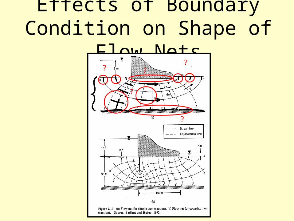
Seepage and Dams
Flow nets for seepage through earthen dams
Seepage under concrete dams
Uses boundary conditions (L & R)
Requires curvilinear square grids for solution
After Philip BedientRice University
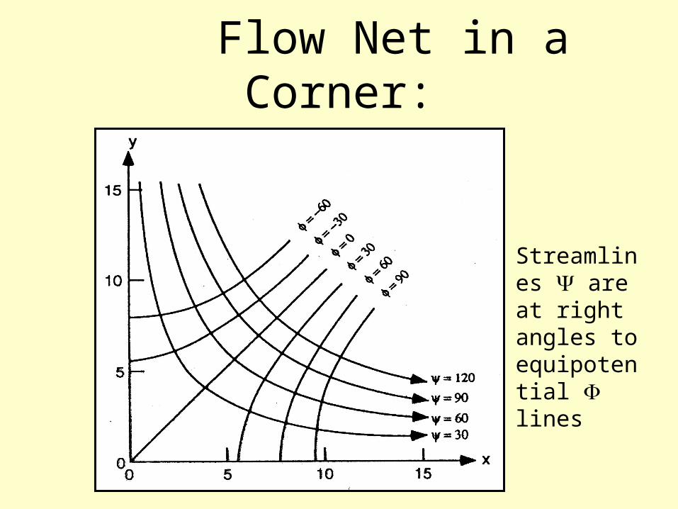
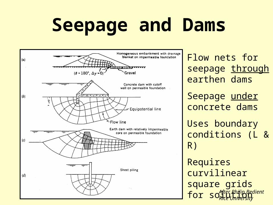
Flow Net in a Corner:
Streamlines are at right angles to equipotential lines
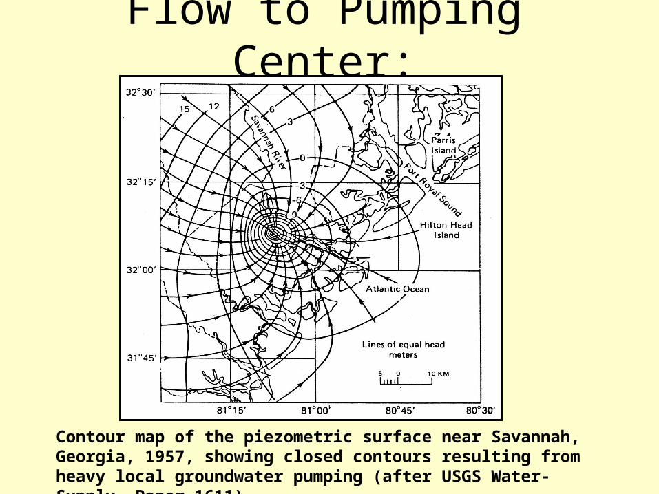
Flow to Pumping Center:
Contour map of the piezometric surface near Savannah, Georgia, 1957, showing closed contours resulting from heavy local groundwater pumping (after USGS Water-Supply Paper 1611).
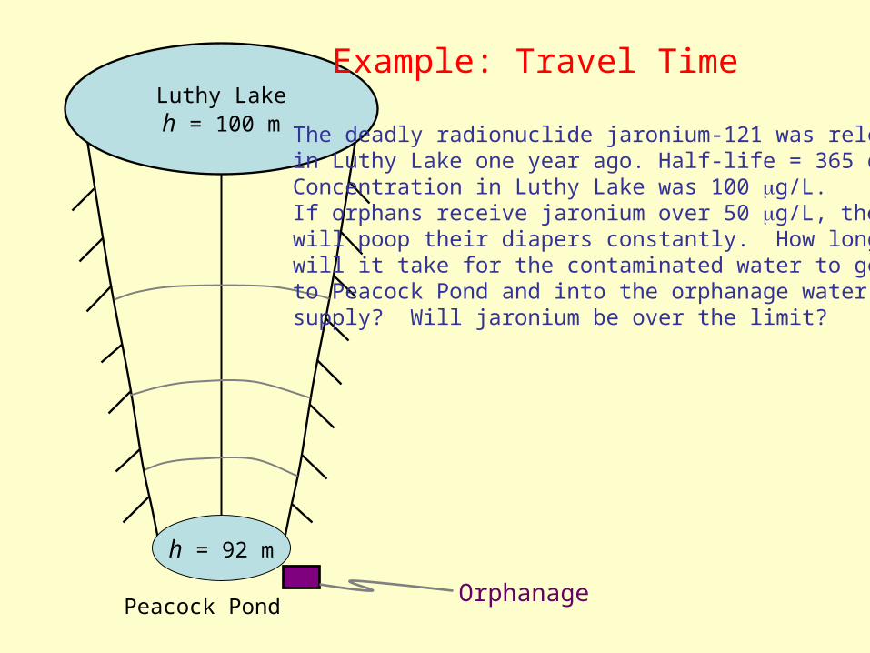
h = 92 m
Luthy Lakeh = 100 m
Peacock PondOrphanage
The deadly radionuclide jaronium-121 was releasedin Luthy Lake one year ago. Half-life = 365 daysConcentration in Luthy Lake was 100 g/L.If orphans receive jaronium over 50 g/L, theywill poop their diapers constantly. How longwill it take for the contaminated water to getto Peacock Pond and into the orphanage watersupply? Will jaronium be over the limit?
Example: Travel Time
Travel time
∑∑∑∑ Δ=
Δ=
Δ=Δ=Δ
4
1
4
1
4
1
4
1
i
i
i
ii
i
iitotal q
ln
q
ln
v
ltt
∑∑ ΔΔ
=Δ=Δ4
1
24
1
iitotal lhK
ntt
ii
i
i
ii l
hK
l
hK
bw
ΔΔ
=ΔΔ
==
h = 92 m
Luthy Lakeh = 100 m
Peacock Pond
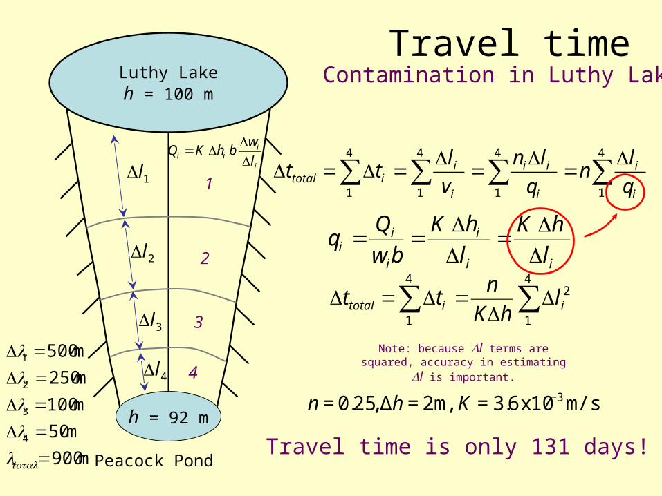
Contamination in Luthy Lake
Travel time is only 131 days!
i
iii l
wbhKQΔΔ
Δ=
€
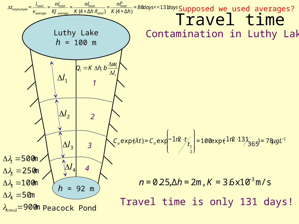
n = 0.25, Δh = 2m, K = 3.6x10⁻³ m/s,
m900
m50
m100
m250
m500
4
3
2
1
==Δ=Δ=Δ=Δ
totallllll
1
2
3
4
2lΔ
1lΔ
3lΔ
4lΔNote: because Δl terms are squared,
accuracy in estimating Δl is important.
Travel time
h = 92 m
Luthy Lakeh = 100 m
Peacock Pond
Contamination in Luthy Lake
Travel time is only 131 days!
i
iii l
wbhKQΔΔ
Δ=
€
n = 0.25, Δh = 2m, K = 3.6x10⁻³ m/s,
m900
m50
m100
m250
m500
4
3
2
1
==Δ=Δ=Δ=Δ
totallllll
1
2
3
4
2lΔ
1lΔ
3lΔ
4lΔ
€
Δttotal simple =ltotal
vaverage
=nltotal
KJaverage
=nltotal
K(4 × Δh / ltotal )=
nltotal2
K(4 × Δh)= 80days <<131days Supposed we used averages?
€
Co exp(−λ t) = Co exp −ln2 ⋅ tt1
2
⎛
⎝
⎜ ⎜
⎞
⎠
⎟ ⎟=100exp(−ln2 ⋅131
365) = 78μgL−1
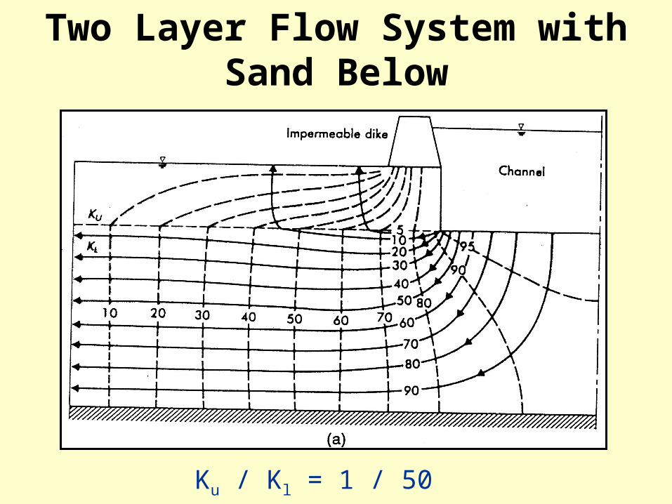
Two Layer Flow System with Sand Below
Ku / Kl = 1 / 50
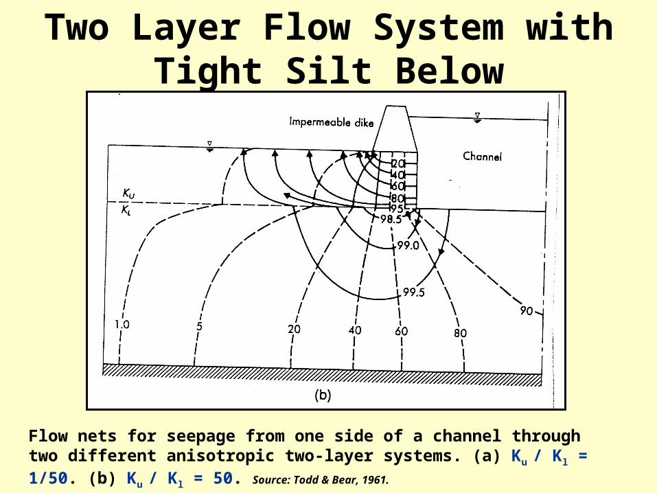
Two Layer Flow System with Tight Silt Below
Flow nets for seepage from one side of a channel through two different anisotropic two-layer systems. (a) Ku / Kl = 1/50. (b) Ku / Kl = 50. Source: Todd & Bear, 1961.
SZ2005 Fig. 5.11
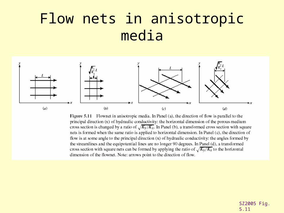
Flow nets in anisotropic media
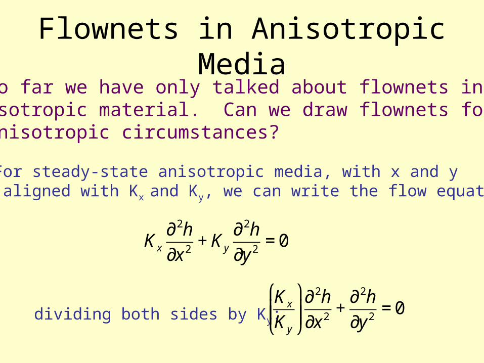
Flownets in Anisotropic MediaSo far we have only talked about flownets in isotropic material. Can we draw flownets foranisotropic circumstances?
€
Kx
∂ 2h
∂x 2+ Ky
∂ 2h
∂y 2= 0
For steady-state anisotropic media, with x and y aligned with Kx and Ky, we can write the flow equation:
dividing both sides by Ky:
€
Kx
Ky
⎛
⎝ ⎜ ⎜
⎞
⎠ ⎟ ⎟∂ 2h
∂x 2+
∂ 2h
∂y 2= 0
Flownets in Anisotropic Media
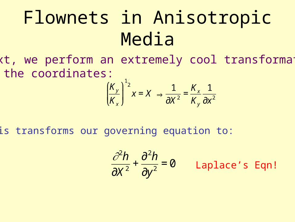
Next, we perform an extremely cool transformationof the coordinates:
€
Ky
Kx
⎛
⎝ ⎜
⎞
⎠ ⎟
12
x = X ⇒1
∂X 2=
Kx
Ky
1
∂x 2
This transforms our governing equation to:
€
∂2h
∂X 2+
∂ 2h
∂y 2= 0 Laplace’s Eqn!
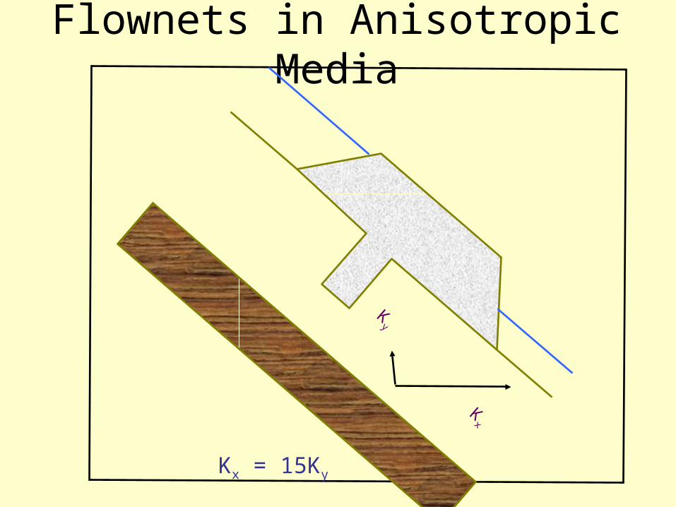
Flownets in Anisotropic Media
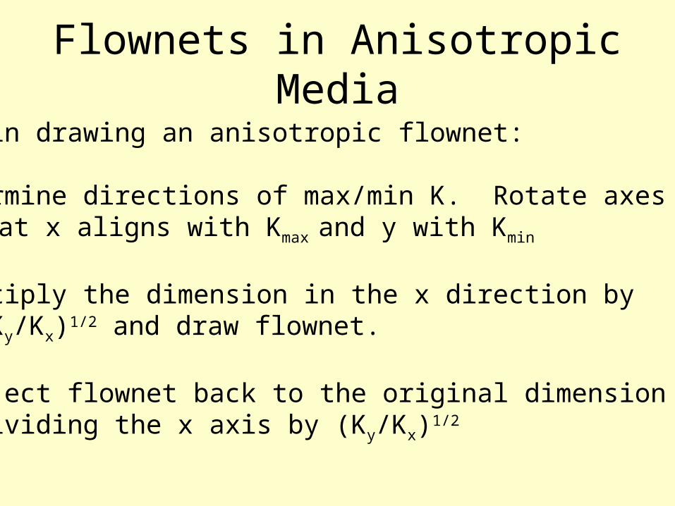
Steps in drawing an anisotropic flownet:
1.Determine directions of max/min K. Rotate axesso that x aligns with Kmax and y with Kmin
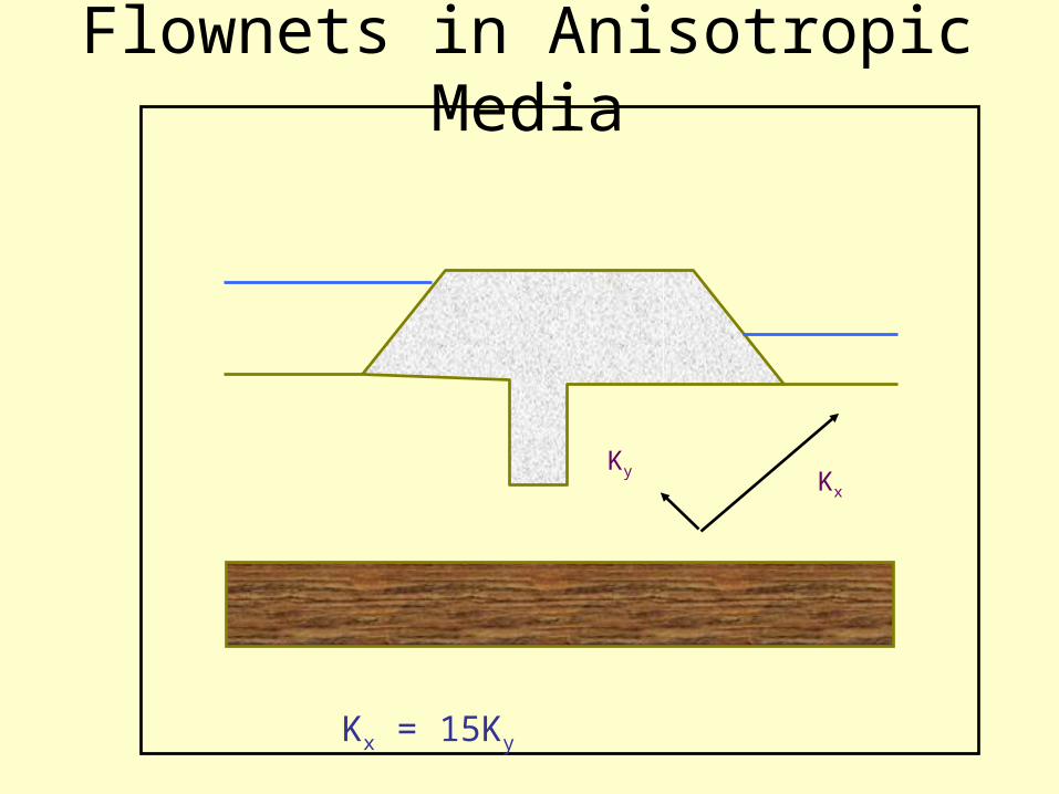
2. Multiply the dimension in the x direction by (Ky/Kx)1/2 and draw flownet.
3. Project flownet back to the original dimension by dividing the x axis by (Ky/Kx)1/2
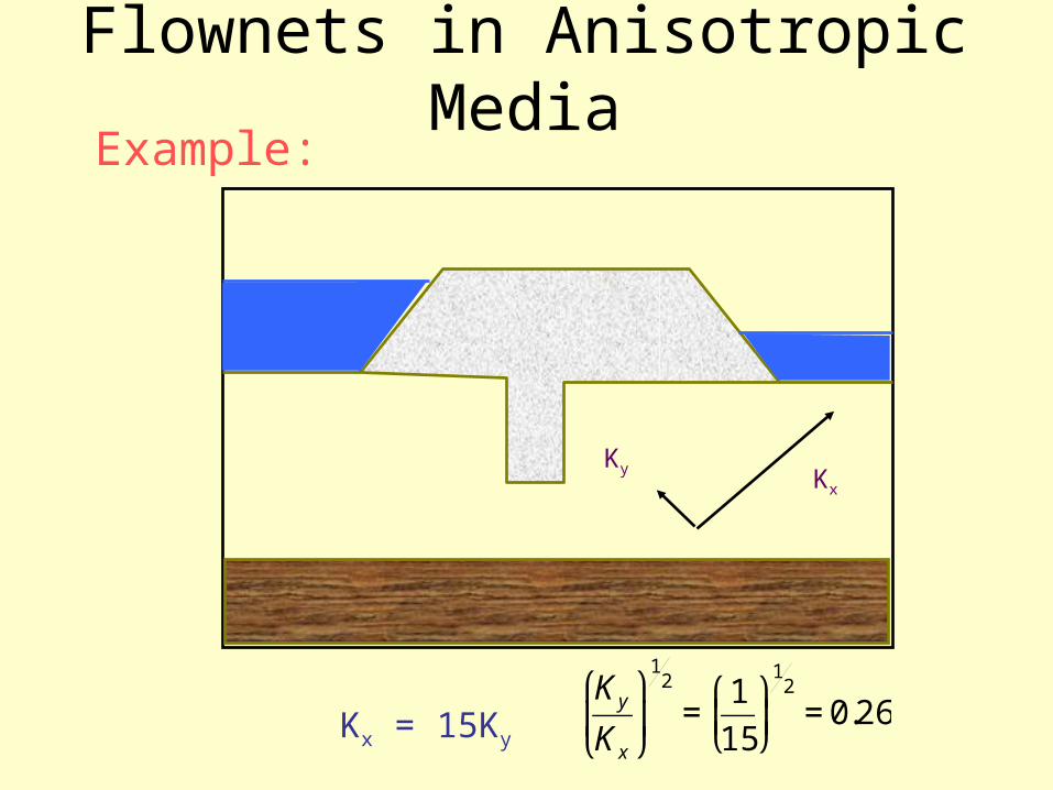
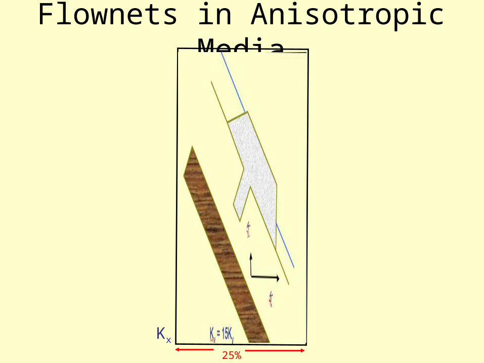
Flownets in Anisotropic MediaExample:
Kx
Ky
Kx = 15Ky
€
Ky
Kx
⎛
⎝ ⎜
⎞
⎠ ⎟
12
=1
15
⎛
⎝ ⎜
⎞
⎠ ⎟1
2
= 0.26
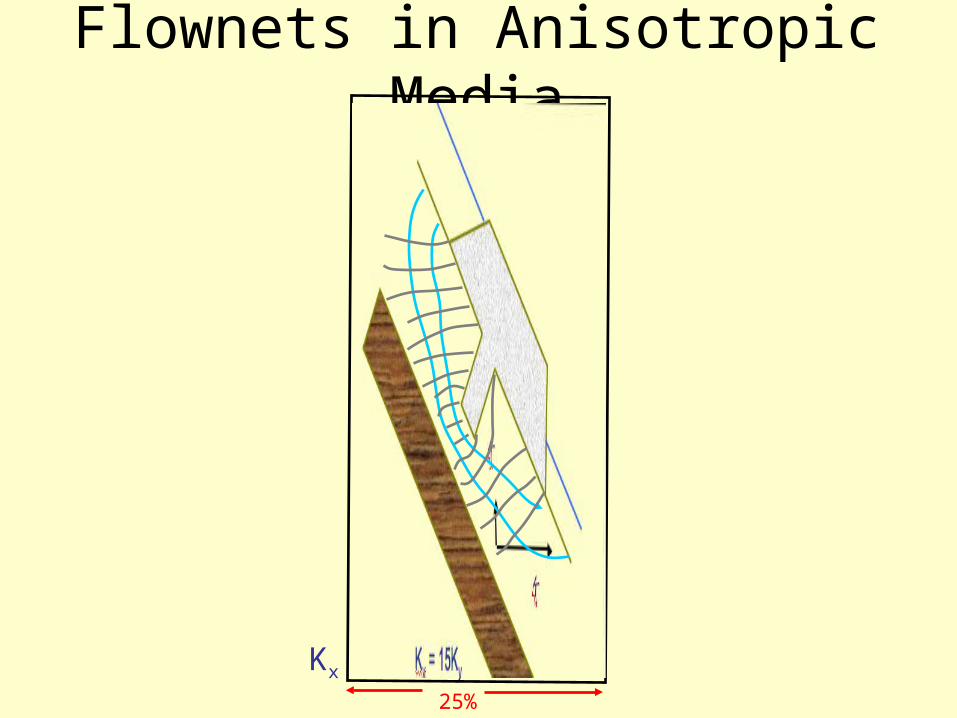
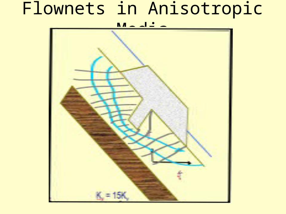
Flownets in Anisotropic Media
Kx
Ky
Kx = 15Ky
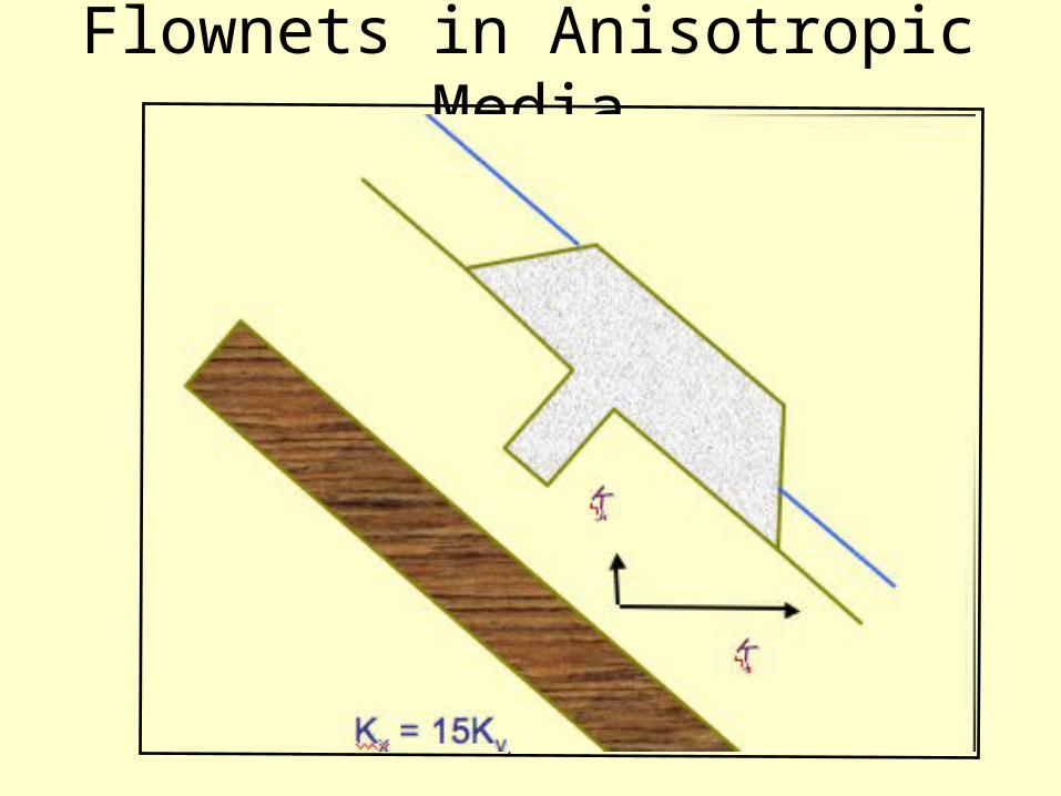
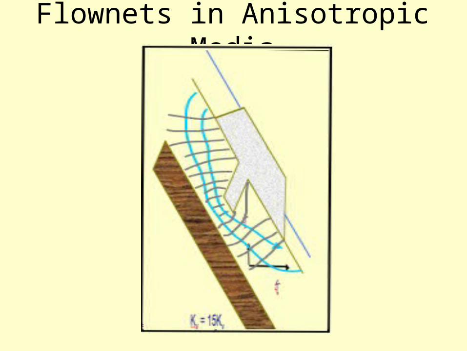
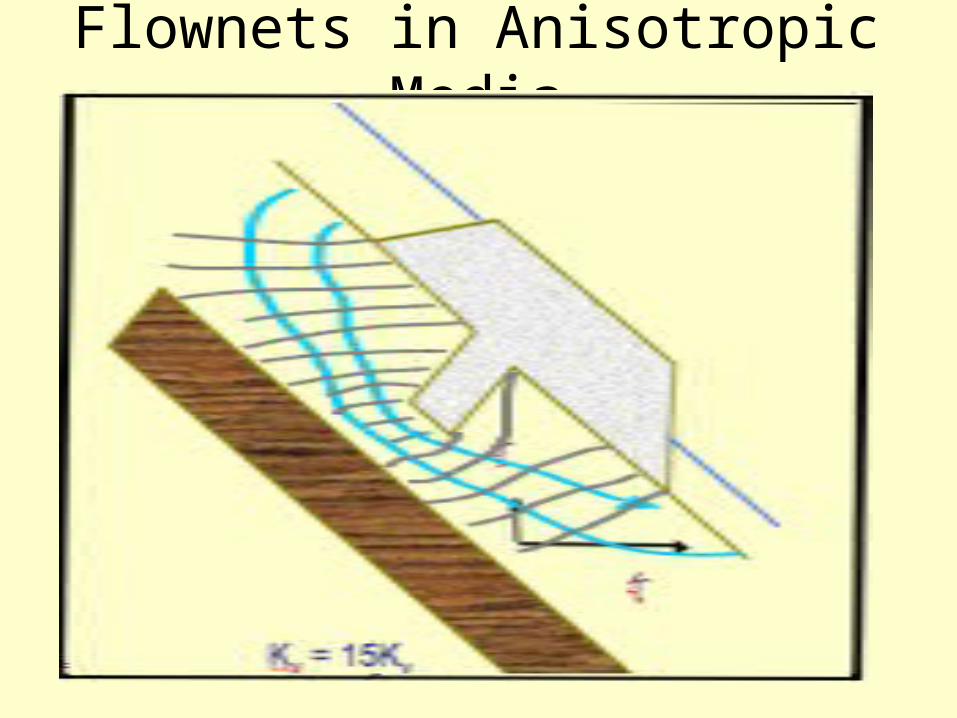
Flownets in Anisotropic Media
Kx
Ky
Kx = 15Ky
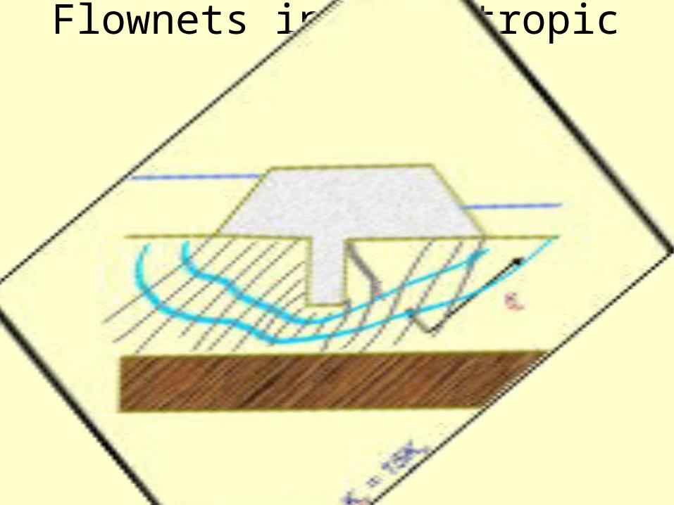
Flownets in Anisotropic Media
Kx = 15Ky
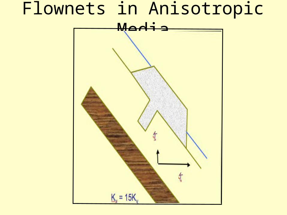
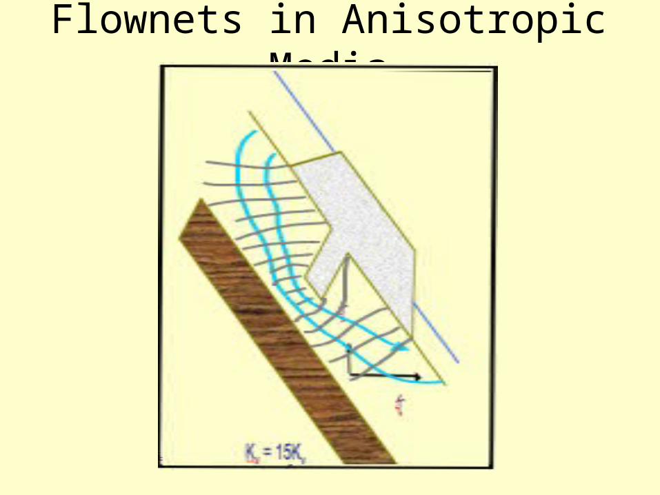
Flownets in Anisotropic Media
Kx = 15Ky
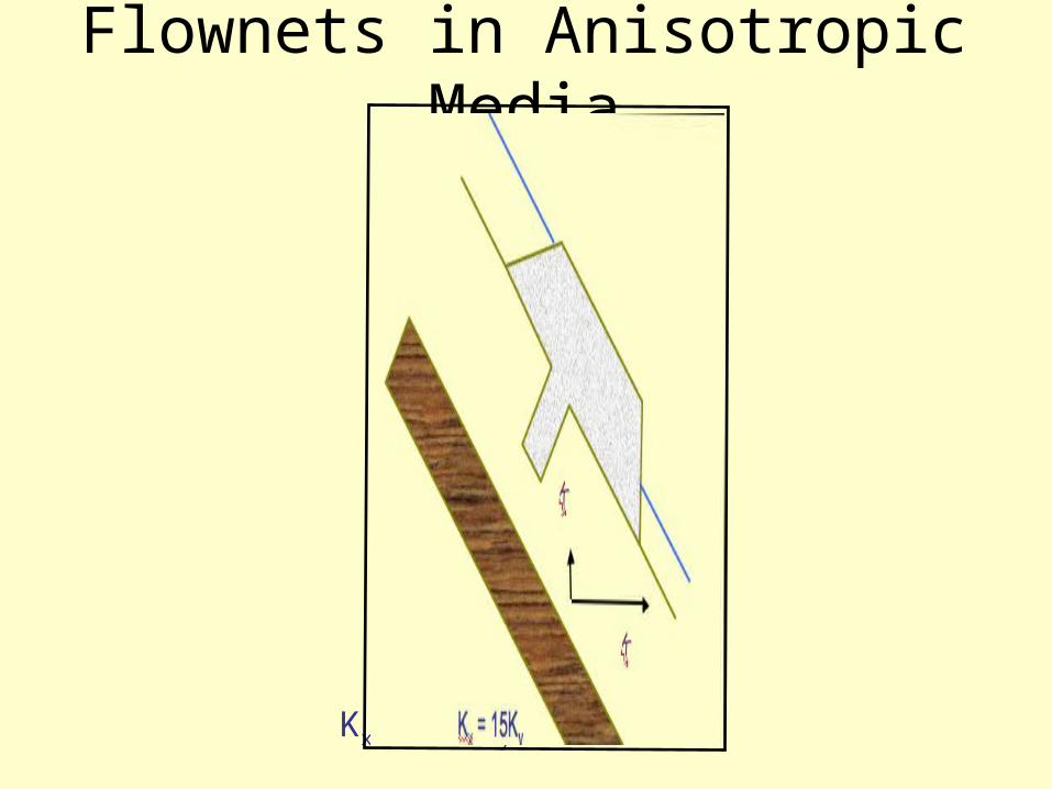
Flownets in Anisotropic Media
Kx = 15Ky
Flownets in Anisotropic Media
Kx = 15Ky
25%
Flownets in Anisotropic Media
Kx = 15Ky
25%
Flownets in Anisotropic Media
Kx = 15Ky
Flownets in Anisotropic Media
Kx = 15Ky
Flownets in Anisotropic Media
Kx = 15Ky
Flownets in Anisotropic Media
Kx = 15Ky
Flownets in Anisotropic Media
Kx = 15Ky
Flow Nets: an example
• A dam is constructed on a permeable stratum underlain by an impermeable rock. A row of sheet pile is installed at the upstream face. If the permeable soil has a hydraulic conductivity of 150 ft/day, determine the rate of flow or seepage under the dam.
After Philip BedientRice University
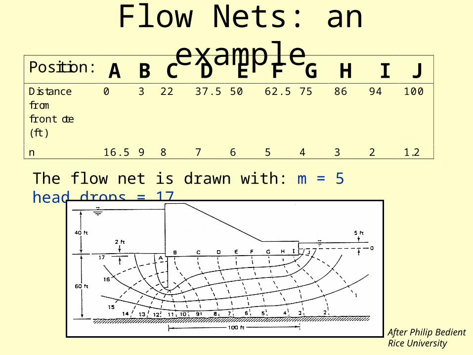
Flow Nets: an examplePosition: A B C D E F G H I JDistancefromfront toe(ft)
0 3 22 37.5 50 62.5 75 86 94 100
n 16.5 9 8 7 6 5 4 3 2 1.2
The flow net is drawn with: m = 5 head drops = 17
After Philip BedientRice University
Flow Nets: the solution
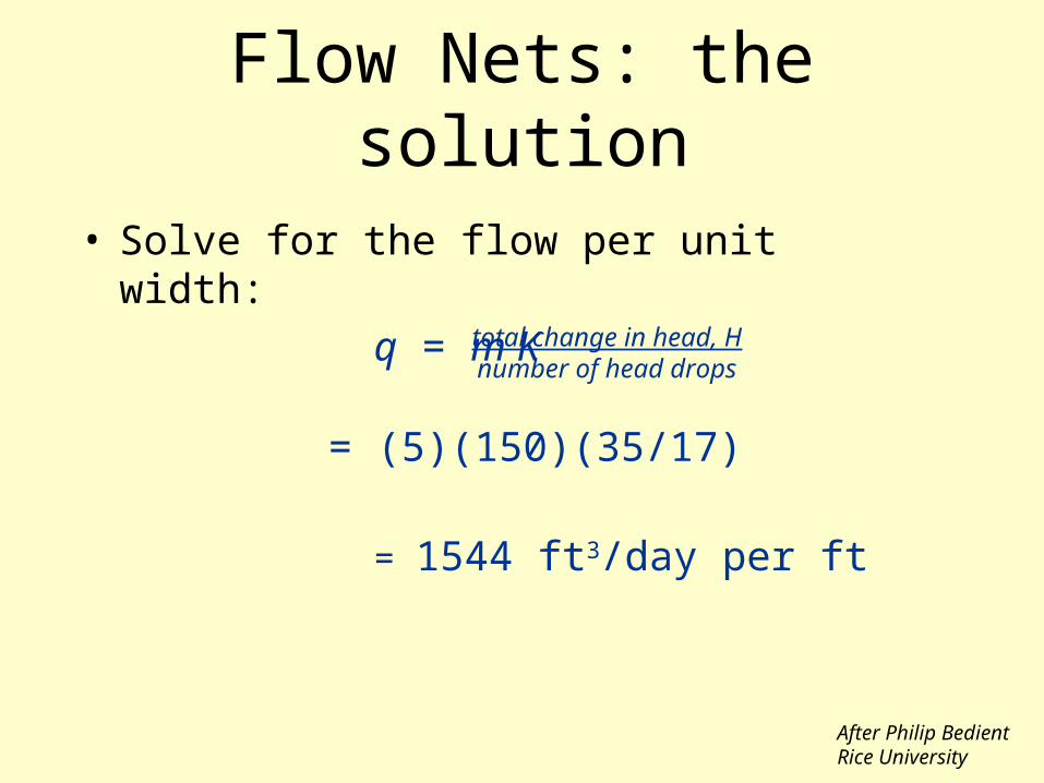
• Solve for the flow per unit width:
q = m K
= (5)(150)(35/17)
= 1544 ft3/day per ft
total change in head, Hnumber of head drops
After Philip BedientRice University
Flow Nets: An Example
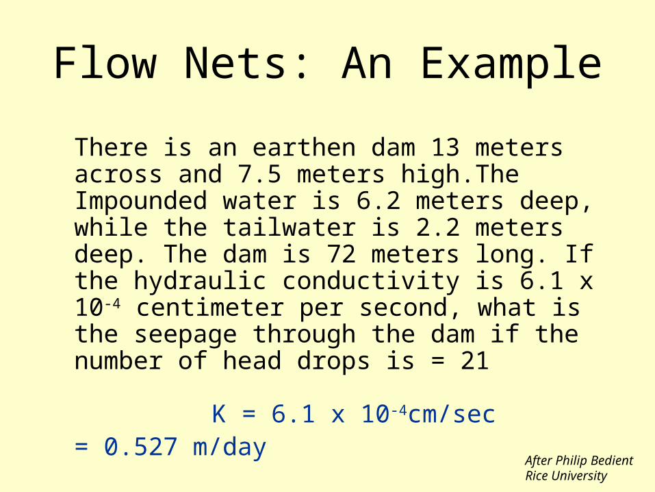
There is an earthen dam 13 meters across and 7.5 meters high.The Impounded water is 6.2 meters deep, while the tailwater is 2.2 meters deep. The dam is 72 meters long. If the hydraulic conductivity is 6.1 x 10⁻⁴ centimeter per second, what is the seepage through the dam if the number of head drops is = 21
K = 6.1 x 10⁻⁴cm/sec= 0.527 m/day After Philip Bedient
Rice University
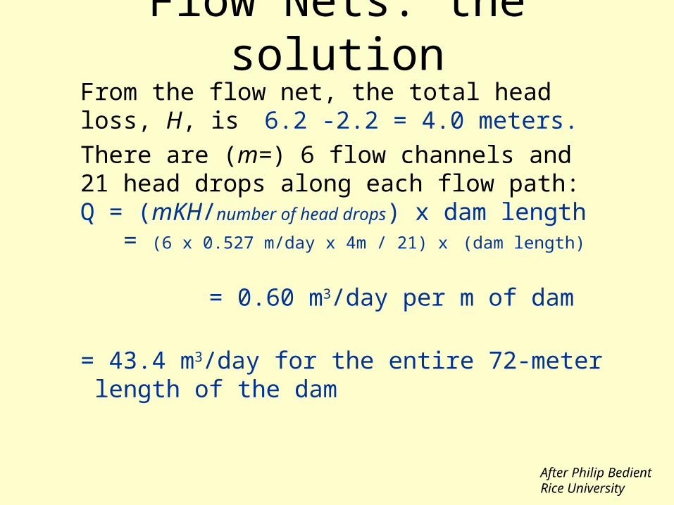
Flow Nets: the solutionFrom the flow net, the total head loss, H, is 6.2 -2.2 = 4.0 meters.There are (m=) 6 flow channels and 21 head drops along each flow path:
Q = (mKH/number of head drops) x dam length = (6 x 0.527 m/day x 4m / 21)
x (dam length) = 0.60 m3/day per m of dam
= 43.4 m3/day for the entire 72-meter length of the dam
After Philip BedientRice University
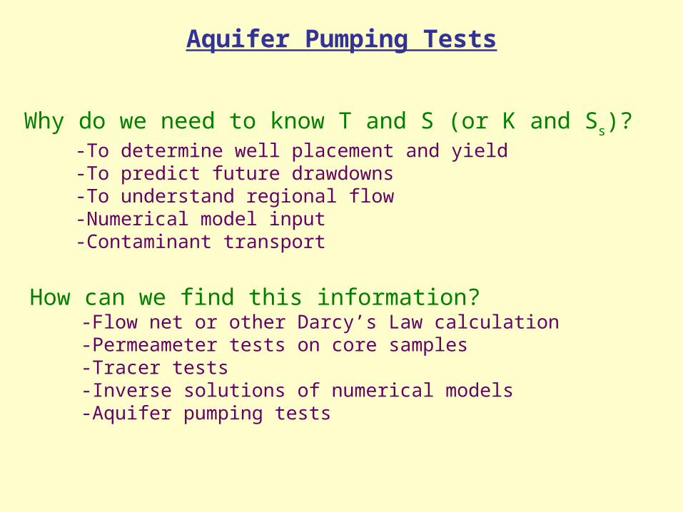
Aquifer Pumping Tests
Why do we need to know T and S (or K and Ss)?-To determine well placement and yield-To predict future drawdowns-To understand regional flow-Numerical model input-Contaminant transport
How can we find this information?-Flow net or other Darcy’s Law calculation-Permeameter tests on core samples-Tracer tests-Inverse solutions of numerical models-Aquifer pumping tests
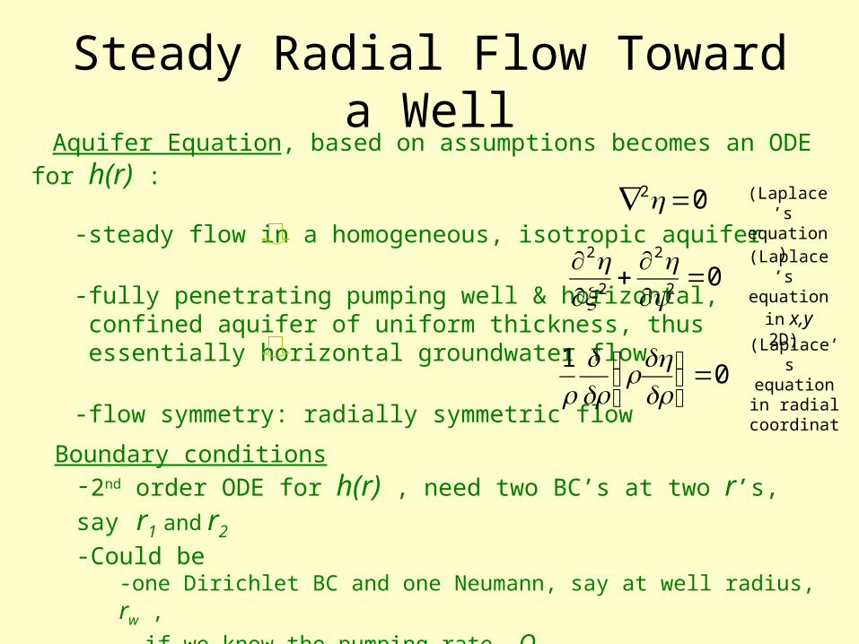
Aquifer Equation, based on assumptions becomes an ODE for h(r) :
-steady flow in a homogeneous, isotropic aquifer
-fully penetrating pumping well & horizontal, confined aquifer of uniform thickness, thus essentially horizontal groundwater flow
-flow symmetry: radially symmetric flow
02 =∇ h (Laplace’s
equation)
01
=⎟⎠⎞
⎜⎝⎛
drdh
rdrd
r
Steady Radial Flow Toward a Well
02
2
2
2
=∂∂
+∂∂
yh
xh (Laplace’s
equation in x,y 2D)
(Laplace’s equation in
radial coordinates)
Boundary conditions-2nd order ODE for h(r) , need two BC’s at two r’s, say r1 and r2
-Could be -one Dirichlet BC and one Neumann, say at well radius, rw ,
if we know the pumping rate, Qw
-or two Dirichlet BCs, e.g., two observation wells.
Steady Radial Flow Toward a Well
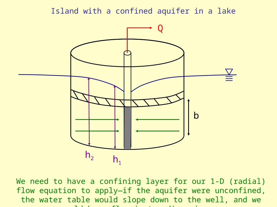
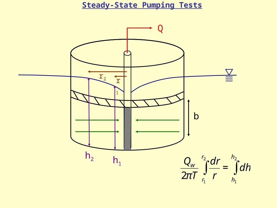
We need to have a confining layer for our 1-D (radial) flow equation to apply—if the aquifer were unconfined, the water table would slope down to
the well, and we would have flow in two dimensions.
b
h1h2
Q
Island with a confined aquifer in a lake
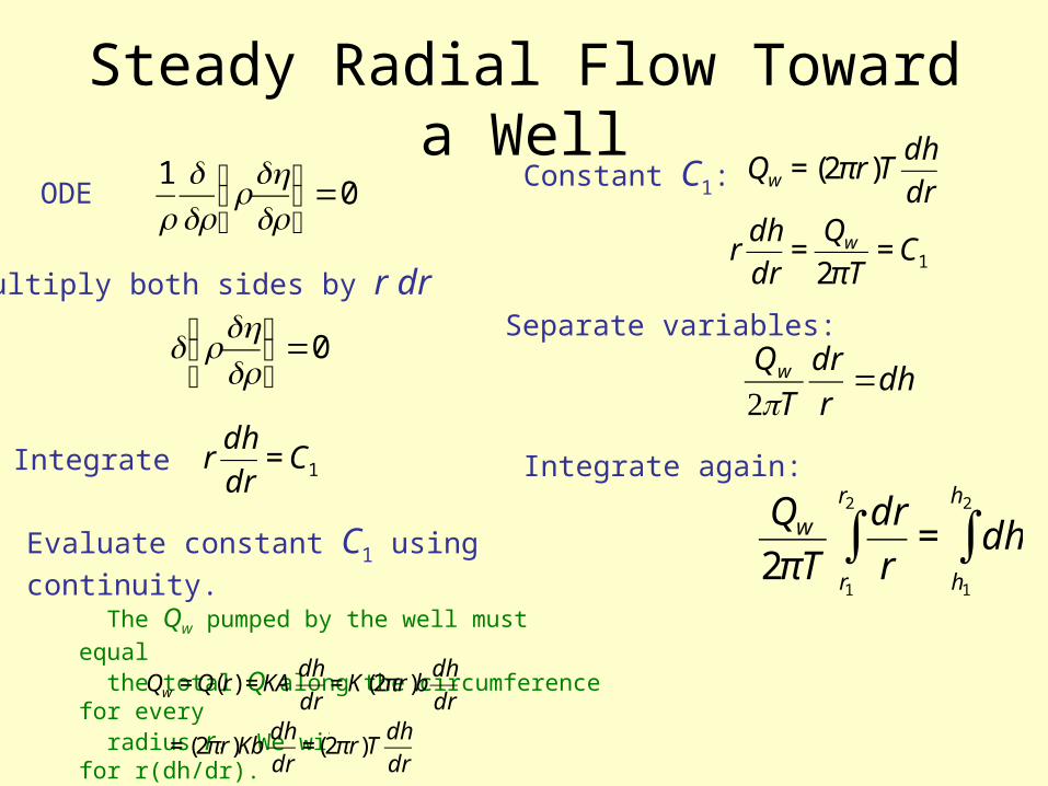
Multiply both sides by r dr
0=⎟⎠
⎞⎜⎝
⎛drdh
rd
Integrate
€
rdh
dr= C1
01
=⎟⎠
⎞⎜⎝
⎛drdh
rdrd
r
Evaluate constant C1 using continuity. The Qw pumped by the well must equal
the total Q along the circumference for every radius r. We will solve Darcys Law for r(dh/dr).
Steady Radial Flow Toward a Well
dhr
dr
T
Qw =π2
ODEConstant C1:
Separate variables:
€
Qw = (2πr)Tdh
dr
rdh
dr=
Qw
2πT= C1
Integrate again:
€
Qw
2πT
dr
rr1
r2
∫ = dhh1
h2
∫
€
Qw = Q(r) = KAdh
dr= K(2πr)b
dh
dr
= (2πr)Kbdh
dr=(2πr)T
dh
dr
b
h1h2
Q
r2 r1
Steady-State Pumping Tests
€
Qw
2πT
dr
rr1
r2
∫ = dhh1
h2
∫
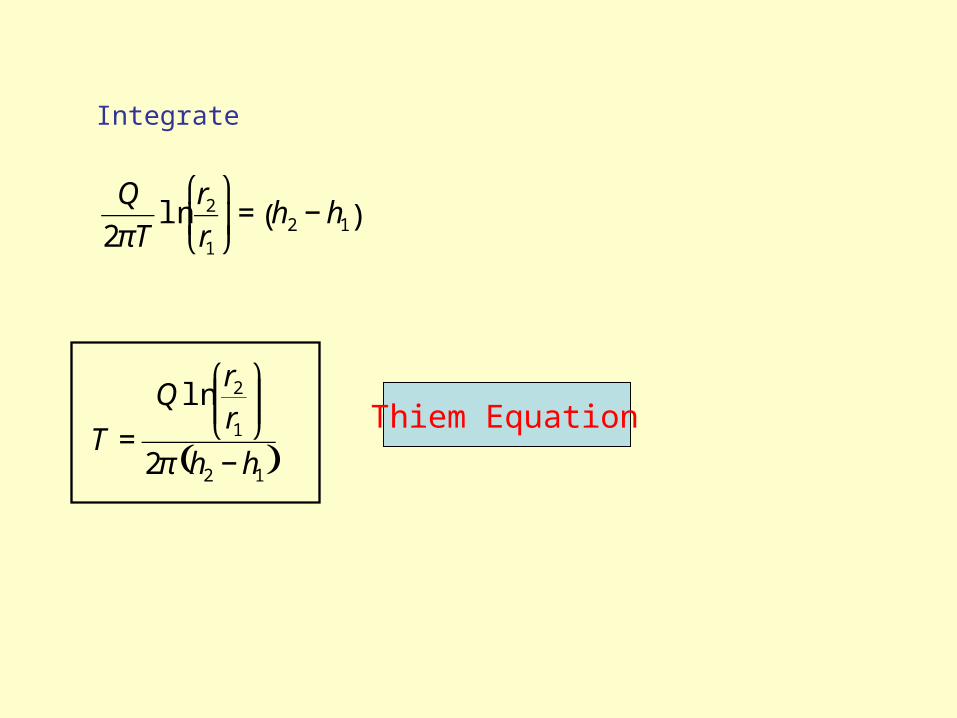
Integrate
€
Q
2πTln
r2
r1
⎛
⎝ ⎜
⎞
⎠ ⎟= h2 − h1( )
( )12
1
2
2
ln
hh
r
rQ
T−
⎟⎟⎠
⎞⎜⎜⎝
⎛
=π
Thiem Equation
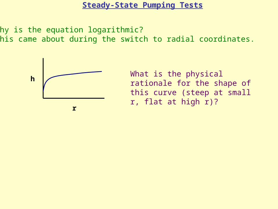
h
r
What is the physical rationale for the shape of this curve (steep at small r, flat at high r)?
Why is the equation logarithmic?This came about during the switch to radial coordinates.
Steady-State Pumping Tests

(Driscoll, 1986)
As we approach the well the rings get smaller. A is smaller but Q is the
same, so must increase. dl
dh
Think of water as flowingtoward the well through a series
of rings.
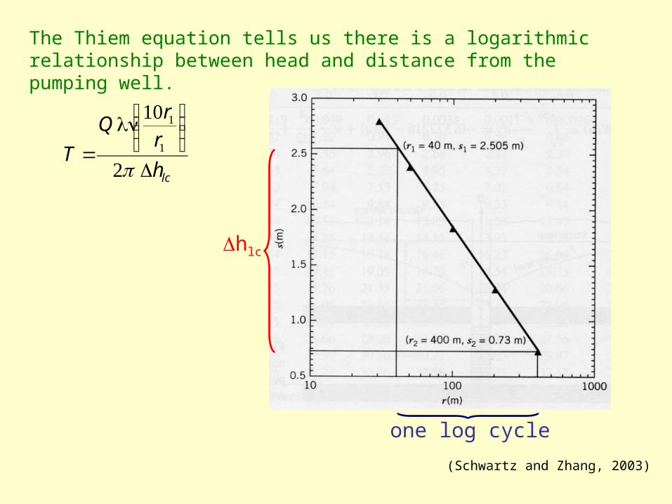
The Thiem equation tells us there is a logarithmic relationship between head and distance from the pumping well.
lch
rr
Q
TΔ
⎟⎟⎠
⎞⎜⎜⎝
⎛
= 2
10ln
1
1
π
hlc
one log cycle
(Schwartz and Zhang, 2003)
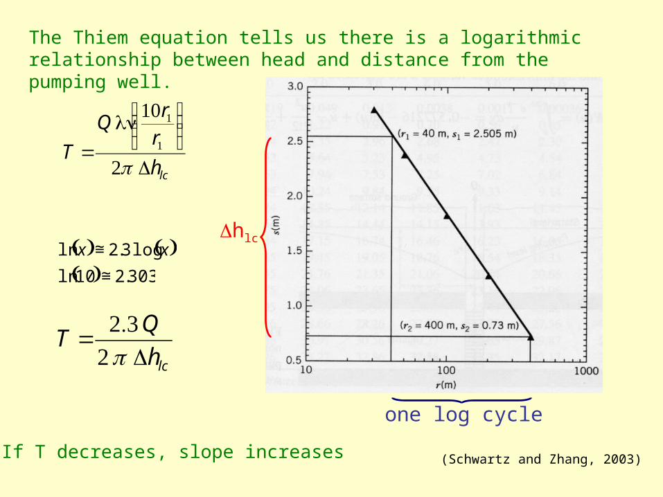
The Thiem equation tells us there is a logarithmic relationship between head and distance from the pumping well.
lch
rr
Q
TΔ
⎟⎟⎠
⎞⎜⎜⎝
⎛
= 2
10ln
1
1
π
( ) ( )xx log 3.2ln ≅
If T decreases, slope increases
lch
QT
Δ=
2 3.2
π
hlc
one log cycle
(Schwartz and Zhang, 2003)
( ) 303.210ln ≅
Steady-State Pumping Tests
Can we determine S from a Thiem analysis?
No—head isn’t changing!