Effects of anisotropic and curvature losses on theoperation of geodesic lenses in Ti:LiNbO3

waveguides

David W. Vahey, Richard P. Kenan, and William K. Burns

The effects of curvature and anisotropy (leaky-mode) losses on the performance of geodesic lenses in Ti-dif-fused waveguides in LiNbO3 are examined. A model for the lenses is developed that is equivalent to the

usual Fraunhofer diffraction theory, modified to account for the path-dependent losses. Numerical calcula-tions show that the curvature losses are dominant and require fabrication of waveguides having well-con-fined fundamental modes. Higher-order modes are effectively attenuated by the lenses. The leaky-modelosses have the beneficial effect of reducing the side-lobe intensity in the focal plane.

1. Introduction

There currently exists considerable interest in thepotential of integrated optical systems for performingoptical data processing functions.1' 2 LiNbO3 is an at-tractive substrate for these systems because of itselectrooptic and acoustooptic capabilities and becauseof the high optical quality of its waveguides. In pro-cessors that require the Fourier-transform capabilitiesof waveguide lenses, such as an integrated opticalspectrum analyzer,1 geodesic lenses3 -5 are employedwith LiNbO3 substrates because of the difficulty ofmaking high-power Luneburg6 or mode-index lenses7

with conventional optical materials.Considerable research has gone toward the correction

of spherical aberrations in geodesic waveguide lensesby means such as aspheric shaping of the lens depres-sion8-10 and forming corrective mode-index overlaysadjacent to the lens.''1 2 These methods have generallymet with some success. However, there are severalphenomena other than spherical aberrations that candegrade geodesic lens performance in a LiNbO3 Fou-rier-transform processor, and these have not yet beenconsidered: leaky-mode loss due to propagation innonaxial propagation directions13' 14 and radiation lossesassociated with the curvature of the lens depression. 5

William Burns is with U.S. Naval Research Laboratory, Wash-ington, D.C. 20375; the other authors are with Battelle ColumbusLaboratories, Columbus, Ohio 43201.

Received 6 July 1979.0003-6935/80/020270-06$00.50/0.C 1980 Optical Society of America.

Because light rays that propagate through differentportions of a geodesic lens experience these loss mech-anisms to different degrees, the amplitude distributionin the back focal plane of the geodesic lens will not bea true Fourier transform of the amplitude distributionin the front focal plane.

The objective of this paper is to study these effectsfor a number of representative waveguides and to de-termine those conditions for which their magnitudes arelarge enough to result in serious problems when the lensis used as a Fourier-transform element in an integratedoptical spectrum analyzer.

II. Theory

A. Modification of the Fourier-Transform Relationship

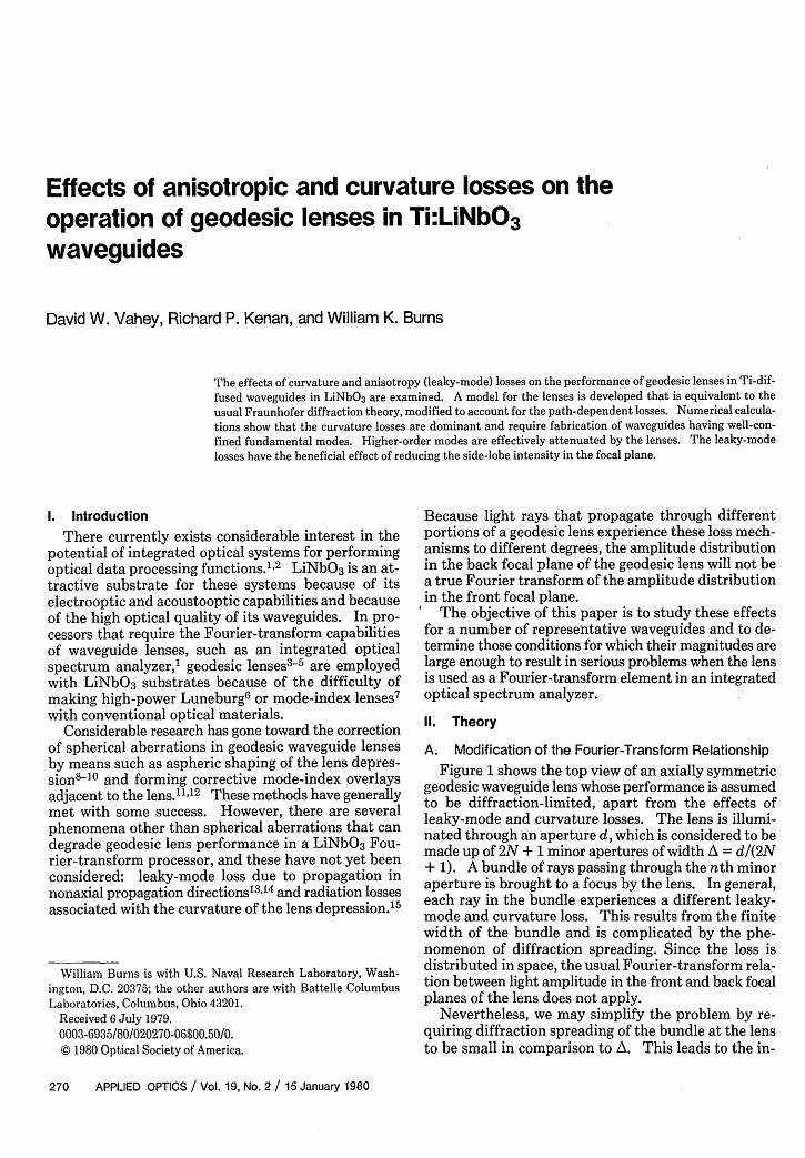
Figure 1 shows the top view of an axially symmetricgeodesic waveguide lens whose performance is assumedto be diffraction-limited, apart from the effects ofleaky-mode and curvature losses. The lens is illumi-nated through an aperture d, which is considered to bemade up of 2N + 1 minor apertures of width A = d/(2N+ 1). A bundle of rays passing through the nth minoraperture is brought to a focus by the lens. In general,each ray in the bundle experiences a different leaky-mode and curvature loss. This results from the finitewidth of the bundle and is complicated by the phe-nomenon of diffraction spreading. Since the loss isdistributed in space, the usual Fourier-transform rela-tion between light amplitude in the front and back focalplanes of the lens does not apply.

Nevertheless, we may simplify the problem by re-quiring diffraction spreading of the bundle at the lensto be small in comparison to A. This leads to the in-

270 APPLIED OPTICS / Vol. 19, No. 2 / 15 January 1980

I le"(X)1

Fig. 1. Geometry for calculating waveguide-curvature losses andleaky-mode propagation losses on geodesic-lens performance.

equality A >> (fX)1/2. If we further require A <<I T(h)/T'(h) min, where T(h) is the over-all amplitudetransmission of the ray incident at height h in travelingthe distance between the front and back focal planes,each ray in the bundle experiences approximately thesame transmission T(h) T(dn) = T, where h = d,describes the position of the central ray of the bundlewe are considering. In view of the nearly uniform losses,it is plausible to ignore their distributed nature andtreat them as though they were confined to the frontfocal plane. We may then write the conventionalFourier-transform relationship for a lens that focusesin one dimension' 6 :

E~(x)= (ify'/ 2d d+A/2

En(x) = (ifX)-/2 JdA/ 2 T(h)A(h) exp(-i27rhx/fX)dh, (1)

where En (x) is the transverse amplitude variation in theback focal plane when A (h) is the amplitude variationin the front focal plane, and T(h) now plays a roleequivalent to that of an input transparency in conven-tional optical processing. If all minor apertures n areilluminated, the total amplitude in the back focal planeis

NE(x) = L_ En(x). (2)

n=-NSubstituting Eq. (1) into Eq. (2), we find for an axiallysymmetric input beam

E(x) = 2(ifX)-1/2 3' T(h)A(h) cos(27rhx/fX)dh. (3)

Although this result is independent of A, recall that werequired both A >> (fX)1/2 and A << T(h)/T'(h) I min forits justification. Combining the two inequalities, weconclude that Eq. (3) is valid when

(fX)1/ 2 << I T(h)/T'(h) min. (4)

For focal lengths of a few centimeters and wavelengthsof a few tenths of a micrometer, (fX)1/2 -100 ,im. Theresults we obtain using Eq. (3) will therefore be validwhen the right-hand side of Ineq. (4) is on the order ofmillimeters. Computed results to be presented arebased on an approximation to Eq. (3) obtained by takingT(h) T(dn) = Tn and A(h) A(d = An in Eq. (1),performing the integral, and applying Eq. (2) to theresult. We find

E(x) = 2(ifX) 1 /2 sincX AOTO/2 + AT,, cos(2irnX)j (5)

where X = xA/fX and sincX = sinrX/7rX. Since thisresult is simply an approximate representation of Eq.(3) suitable for numerical computation, we are no longerbound by the constraint A >> (fX)1/2, and, in fact, theprecision of Eq. (5) improves as A becomes increasinglysmall.

B. Determination of the Amplitude TransmissionFunction T(h)

The function T(h) describes the reduction of ampli-tude experienced by a ray passing from the front focalplane to the back focal plane when the initial height ofthe ray relative to the beam axis is h. It may be con-veniently written as the product of three transmissionfunctions:

T(h) = T1(h)T2(h)T 3(h), (6)

where Ti (h) is the transmission associated with leaky-mode propagation losses outside the lens depression,T 2 (h) is associated with leaky-mode propagation lossesinside the lens depression, and T3(h) is associated withwaveguide-curvature losses inside the lens depression.In each case we may write

Ti(h) = exp [-0.5 f ai(hs)dsj , (7)

where cai (h,s) is the power attenuation coefficient, ands is a variable of integration along the appropriate raypath c.

For losses outside the lens depression, the ray pathc = cut is a straight line extending from the lens rim tothe focus. Leaky-mode propagation losses are constantfor straight trajectories; consequently ail(h,s) = l(h)independent of position along the line.

For losses inside the lens depression, the ray path cindescribes a geodesic curve of the depression surface. Ateach point s, the ray trajectory relative to the crystallineaxes of the LiNbO3 substrate is unique. The leaky-mode attenuation 2(h,s) is sensitive to crystal orien-tation relative to the ray trajectory and hence is acomplicated function of s.1 3,1 4

Dependence of 3(h,s) on s results from the fact thatthe radius of curvature of the depression surface is notconstant, at least for the interesting case of lenses cor-rected by aspheric shaping.8-10

We choose to simplify the analysis by employing s-independent functions ca2(h) and a3(h) that are ex-pected to be close to the average attenuations over thegeodesic path. Thus,

Ti(h) exp[-0.5 (h)1i(h),

1i (h) =fS ds,

c = Cout, i = 1, (8)

c = cin, i = 2,3.

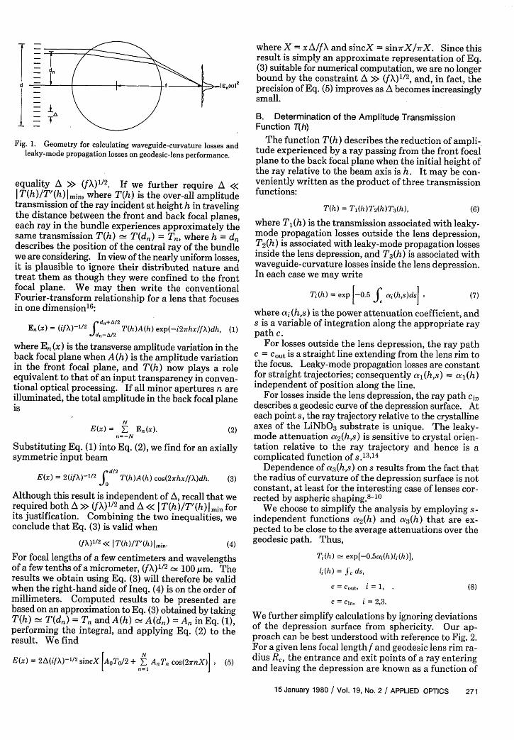
We further simplify calculations by ignoring deviationsof the depression surface from sphericity. Our ap-proach can be best understood with reference to Fig. 2.For a given lens focal length f and geodesic lens rim ra-dius R, the entrance and exit points of a ray enteringand leaving the depression are known as a function of

15 January 1980 / Vol. 19, No. 2 / APPLIED OPTICS 271

ray height h by virtue of the symmetry of the depres-sion. By approximating the depression as a segmentof a spherical surface of radius

R = 2f [R,/(4f - Rc)]1/2, (9)

as determined by the theory of Ref. 3, we find the arclength of the geodesic curve appropriate to the input rayheight h to be

12 13 = 2R sin-'[(R,/R) cos(i -/2)1,

0i = sin-'(h/R.), (10)

A = sin'1(h/f).

To calculate the attenuation coefficient a2 (h) asso-ciated with leaky-mode propagation in the depressionwe take as an average ray trajectory that formed byconnecting the entrance and exit points in the circularlens rim in Fig. 2. By taking the projection of the lensin the horizontal plane we are, in effect, neglecting thelens curvature. The projection of the ray path in thehorizontal plane is still a curve, so we further approxi-mate it by a straight line connecting the entrance andexit points, which should approximate the averagetrajectory for the actual projection. This gives us auniquely defined ray direction (/2 in Fig. 2) in a planecontaining the optic axis, so that the results of Ref. 13can be unambiguously applied. In this context, how-ever, they are approximations that only become correctin the limit of vanishing lens curvature. For the prac-tically important case of an incident beam propagatingperpendicular to the c axis, we have for TE modes'3

_ 4(n2- n2)1/2 sin2i/2;

ncos4'/2

[D(- inb)1/2 + ko1(2Ann b(-'/

= sin'1h/f,

where (7r - 4)/2 is the angle made by the average raytrajectory relative to the c axis, while in the lens de-pression, n (ne) is the ordinary (extraordinary) re-fractive index, An is the maximum index perturbationassociated with the waveguide, b is the normalized modeindex (0 b < 1),17,18 D is the diffusion length of the(assumed) Gaussian diffusion profile, and ko = 2r/Xois the magnitude of the free-space wave vector.

From Eq. (11) we see that the leaky-mode loss can beconsidered as the product of two factors. The first isdirection dependent and increases with 4 and h; thesecond depends only on the waveguide fabrication andmode-depression parameters b, D, and An.

Equation (11) is used to calculate the attenuationcoefficient for leaky-mode propagation outside as wellas inside the lens depression once allowance is made forchanges in the ray trajectory. Since the angle made byrays leaving the depression relative to the normal to thec axis changes from 4/2 to 4, al(h) is obtained by re-placing 4/2 by 4 in Eq. (11). The path length betweenthe lens, rim and the focal point, also needed for thecalculation of transmission TA (h), is

11(h) = V - R, cos(oi - )]/cos*. (12)

For the c-axis orientation shown in Fig. 2, there is noleaky-mode attenuation for rays before they enter thelens. Consequently, the only remaining attenuationcoefficient is a3 (h), for radiation losses associated withlens curvature. We employ Eq. (32) of Marcuse1 9 forradiation losses in cylindrically contoured waveguideswith propagation perpendicular to the cylinder axis.The formula is modified for use with diffused wave-guides by replacing the step-index-waveguide thicknessby the distance from the waveguide surface to theturning point, which for a Gaussian index profile is givenby D(-lnb) 1 /2 . 13 Also, certain approximations that arevalid in the limit An/ne << 1 and 4 - 0 are used tosimplify the form of the result. Using the notation ofEq. (11), we find

2(2Anb/ne)1 2(1 - b)

D(-lnb)1/ 2 + ho1(2Afnneb)-1/2 expg(R)]

g(R) = ko(2Anneb)1/ 2[D(-1nb)1/ 2 - 4/nbR/3ne]. (13)

In this expression R, the radius of curvature of the de-pression, is given by Eq. (9). In view of our neglect ofany asphericity in the depression surface, all rays travelalong great-circle paths and experience the same cur-vature R. Consequently, 3 is independent of h.However, T3(h) depends on ray height by virtue of thepath length 13, given in Eqs. (10). As a result, curvatureradiation losses are largest for rays passing through thecenter of the lens and decrease as h increases. This isin contrast to the situation that exists in the case ofleaky-mode losses.

Equations (5) through (13) of this section must becombined to determine the net transmission coefficientT(h), to be used in Eq. (4) for the electric-field distri-bution in the back focal plane of the geodesic lens.Parameters that must be specified are lens focal lengthf and rim radius Rc, and waveguide parameters An, b,and D. The back focal-plane amplitude distributionE(X) also depends on the input distribution A(h) andon the lens aperture d.

Ill. Analysis

A. Choice of Parameters

Current interest in optical geodesic waveguide lensesin LiNbO3 substrates centers on their application tointegrated acoustooptical spectrum analysis.1 Lenseshaving focal lengths in the 1-2-cm range operating at

I hrn - Axis1 h v

Fig. 2. Geometry for calculating ray attenuations and path

lengths.

272 APPLIED OPTICS / Vol. 19, No. 2 / 15 January 1980

-f/2 and focal lengths in the 5-10-cm range operatingat f/20 may be useful for this application. We an-ticipate that the deleterious effects of leaky-modepropagation and waveguide-curvature radiation losseswill be most severe in the case of short-focal-length,low-f/No. lenses. Therefore we concentrate on thislimit by selecting for examination the case f = 1.0 cm,R = 0.5 cm, and d = (2/3) cm (f/11.5 performance).

Waveguides for use in a spectrum analyzer willprobably be single mode, having 0 < b 0.4. Valuesof b are related to An and D by the theory of Ref. 17. Inturn An and D are related to waveguide fabricationparameters r, T, and t by the process of diffusion. isthe initial thickness of Ti metal diffused into a LiNbO3substrate for a time t at temperature T to make awaveguide.20,21 For y-cut waveguides formed duringa 6-h diffusion at 10000C, the average diffusion depthis D 2.15 gm.22 At this temperature, a working em-pirical relationship that connects the diffusion depthand the initial Ti film thickness to the extraordinaryindex change is22

Ane 1.08(T/D),

so that for D = 2.15 gim, we have

Ane 5.04 X 10 5 T (A).

(14a)

(14b)

Through the use of Eqs. (14) and universal curvesrelating the normalized mode index b to the normalizedwaveguide depth, 1 7

V k0 D(2neAn)1/ 2, (15)

we can compute appropriate values of An and r for se-lected values of b and D. This provides us with all theinformation required to calculate leaky-mode andcurvature-loss coefficients. We select for study the fourwaveguides whose parameters are listed in Table I,where we assume Gaussian diffusion profiles and X0 =0.83gm. The b values for these waveguides span therange from b = 0.1 for weak guides close to cutoff to b= 0.4 for strong guides close to multimode. Also indi-cated in Table I are the film thickness that must bediffused for 6 h at 10000C to generate the required mode

Table 1. Parameters for Waveguides Used In Lens Calculations (X0 =0.83 )m)

b V D(gtm) Ane T (A)0.1 2.52 2.15 0.0055 1090.2 2.98 2.15 0.0077 1530.3 3.55 2.15 0.0109 2160.4 4.30 2.15 0.0161 319

characteristics. Note that the choice of diffusion pa-rameters to obtain a given mode parameter b is notunique. Two different treatments associated with thesame value of b will have different values of An and Dand consequently different leaky-mode and curva-ture-loss characteristics. In turn, these will result invaried geodesic-lens performance characteristics. Itshould be kept in mind that our results and subsequentdiscussion are relevant only for the particular wave-guides described by the parameters of Table I. The factthat these parameters are tied to experimental resultsis therefore appropriate.

B. Ray Transmission Characteristics

To illustrate the relative importance of leaky-modeand curvature losses, we present in Table II the largestand smallest values of leaky-mode and curvature raytransmission for each of the selected waveguides. Indecibels of power, the values tabulated are

TLMI max = 20 logiOTi(0)T2 (0) = 0,

TLM mi. = 20 logioT, (d/2) T2 (d/2),

TCImin = 20 logloT 3 (0),

TCImax = 20 logloT 3 (d/2),

(16)

where TLM and TC refer to leaky-mode and curvaturetransmission, respectively. Calculations are made forthe axial ray h = 0, where TLM is maximum and T isminimum, and for the extremal ray h = d/2, where thereverse situation applies.

Table II shows that curvature losses dominate for b= 0.1 and 0.2, while leaky-mode losses dominate for b= 0.3 and 0.4. The magnitude of the curvature lossesis such that they are virtually intolerable for the smallervalues of b and virtually negligible for the larger valuesof b. The extreme range over which curvature lossesvary results from the exponential factor in the formula,for the curvature attenuation coefficient [Eqs. (13)].Leaky-mode losses show a much smaller range of vari-ation as b varies from 0.1 to 0.4. Yet values for theleaky-mode losses experienced by the extremal ray areseen to be significant in every case, at least for the f/1.5lens we have chosen to examine.

C. Lens Focal CharacteristicsThe results of Table II are qualitatively useful for

indicating the loss of light associated with the leaky-mode and curvature radiation effects. However, lensfocal characteristics depend importantly on the mannerin which the losses are distributed across the lens ap-erture.

Table II. Maximum and Minimum Ray Transmissions Associated with Leaky-mode (LM) and Curvature (C) Losses

b Afne D(,um) TLMImax (dB) TLMImin (dB) TcImax (dB) TcImin (dB)

0.1 0.0055 2.15 0 -1.70 -345.1 -419.30.2 0.0077 2.15 0 -2.92 -35.2 -42.70.3 0.0109 2.15 0 -4.52 -0.01 -0.010.4 0.0161 2.15 0 -6.97 -0.00 -0.00

15 January 1980 / Vol. 19, No. 2 / APPLIED OPTICS 273

-

l-_

.E

0

1,-

b0O.l

0.2

0.: 0.4 0.4

0.0 0.2 ..4 . a.a 1.oNormalized Ray Height, 2h/d

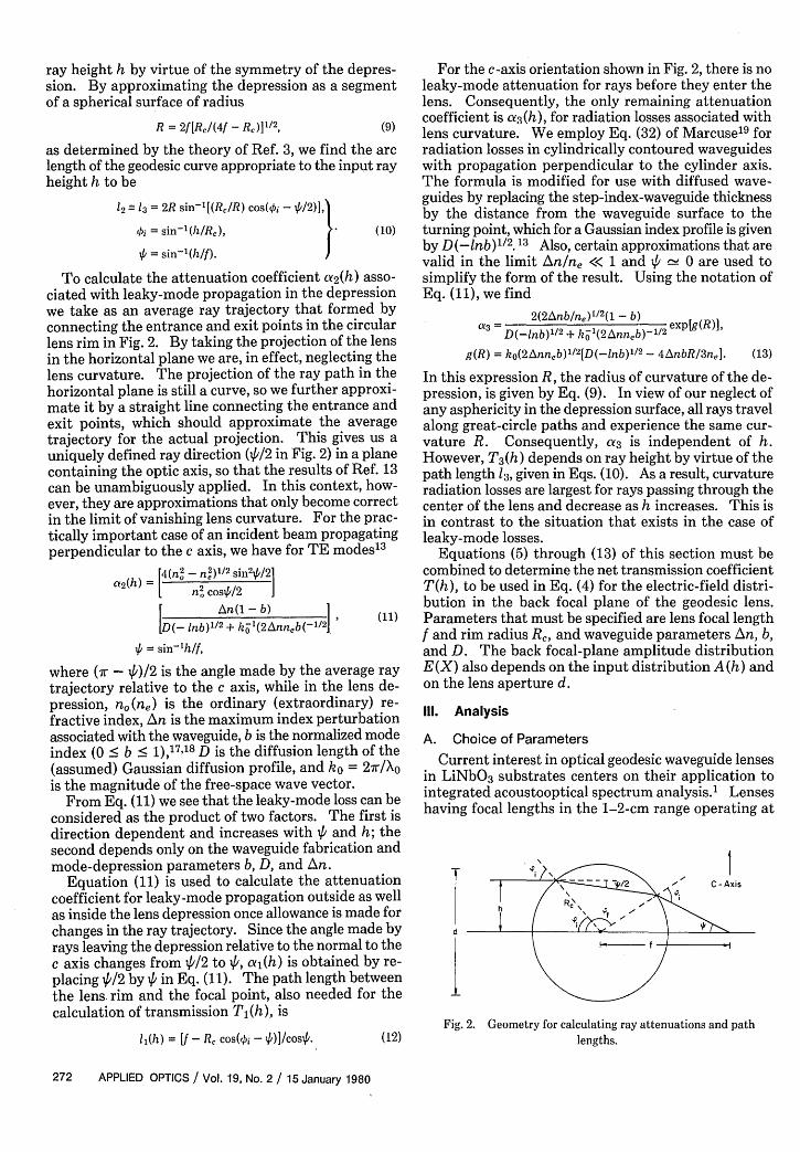
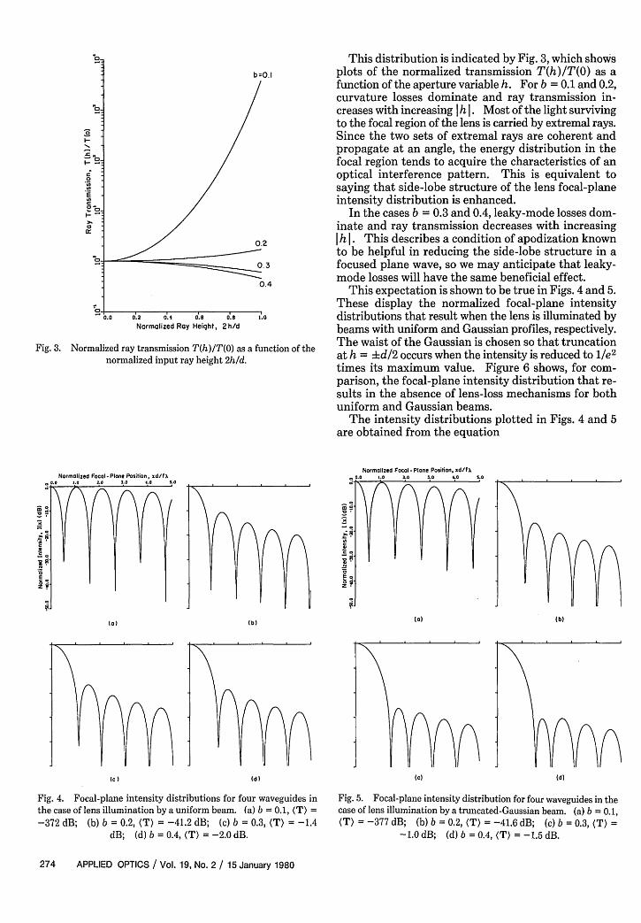
Fig. 3. Normalized ray transmission T(h)/T(0) as a function of thenormalized input ray height 2h/d.

(a) IbI

Ic ) (d)

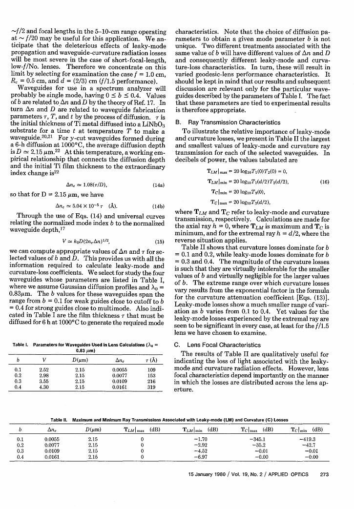
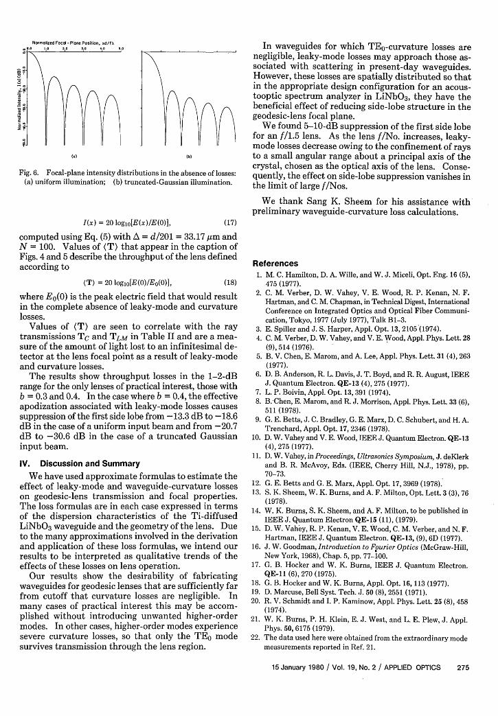
Fig. 4. Focal-plane intensity distributions for four waveguides inthe case of lens illumination by a uniform beam. (a) b = 0.1, (T) =-372 dB; (b) b = 0.2, (T) = -41.2 dB; (c) b = 0.3, (T = -1.4

dB; (d) b = 0.4, (T) = -2.0 dB.

This distribution is indicated by Fig. 3, which showsplots of the normalized transmission T(h)/T(0) as afunction of the aperture variable h. For b = 0.1 and 0.2,curvature losses dominate and ray transmission in-creases with increasing I h 1. Most of the light survivingto the focal region of the lens is carried by extremal rays.Since the two sets of extremal rays are coherent andpropagate at an angle, the energy distribution in thefocal region tends to acquire the characteristics of anoptical interference pattern. This is equivalent tosaying that side-lobe structure of the lens focal-planeintensity distribution is enhanced.

In the cases b = 0.3 and 0.4, leaky-mode losses dom-inate and ray transmission decreases with increasingIh 1. This describes a condition of apodization knownto be helpful in reducing the side-lobe structure in afocused plane wave, so we may anticipate that leaky-mode losses will have the same beneficial effect.

This expectation is shown to be true in Figs. 4 and 5.These display the normalized focal-plane intensitydistributions that result when the lens is illuminated bybeams with uniform and Gaussian profiles, respectively.The waist of the Gaussian is chosen so that truncationat h = Ad/2 occurs when the intensity is reduced to l/e2

times its maximum value. Figure 6 shows, for com-parison, the focal-plane intensity distribution that re-sults in the absence of lens-loss mechanisms for bothuniform and Gaussian beams.

The intensity distributions plotted in Figs. 4 and 5are obtained from the equation

Normalized Focal-Plane Position, nd/fX0.0 '.O 2.0 ° .0 4.0 5.

ca a

-

E

E .

O O

(a)

(c)

(b)

{d)

Fig. 5. Focal-plane intensity distribution for four waveguides in thecase of lens illumination by a truncated-Gaussian beam. (a) b = 0.1,(T) = -377 dB; (b) b = 0.2, (T) = -41.6 dB; (c) b = 0.3, (T) =

-1.0 dB; (d) b = 0.4, (T) = -1.5 dB.

274 APPLIED OPTICS / Vol. 19, No. 2 / 15 January 1980

0

m

Normalized Focal - Plane Position, d/f.. .0 0.0 3.0 :0 5;0

n (b)

Fig. 6. Focal-plane intensity distributions in the absence of losses:(a) uniform illumination; (b) truncated-Gaussian illumination.

I(x) = 20 logio[E(x)/E(0)], (17)

computed using Eq. (5) with A = d/201 = 33.17 gm andN = 100. Values of (T) that appear in the caption ofFigs. 4 and 5 describe the throughput of the lens definedaccording to

(T) = 20 logio[E(0)/Eo(0)], (18)

where Eo(0) is the peak electric field that would resultin the complete absence of leaky-mode and curvaturelosses.

Values of (T) are seen to correlate with the raytransmissions Tc and TLM in Table II and are a mea-sure of the amount of light lost to an infinitesimal de-tector at the lens focal point as a result of leaky-modeand curvature losses.

The results show throughput losses in the 1-2-dBrange for the only lenses of practical interest, those withb = 0.3 and 0.4. In the case where b = 0.4, the effectiveapodization associated with leaky-mode losses causessuppression of the first side lobe from -13.3 dB to -18.6dB in the case of a uniform input beam and from -20.7dB to -30.6 dB in the case of a truncated Gaussianinput beam.

IV. Discussion and SummaryWe have used approximate formulas to estimate the

effect of leaky-mode and waveguide-curvature losseson geodesic-lens transmission and focal properties.The loss formulas are in each case expressed in termsof the dispersion characteristics of the Ti-diffusedLiNbO3 waveguide and the geometry of the lens. Dueto the many approximations involved in the derivationand application of these loss formulas, we intend ourresults to be interpreted as qualitative trends of theeffects of these losses on lens operation.

Our results show the desirability of fabricatingwaveguides for geodesic lenses that are sufficiently farfrom cutoff that curvature losses are negligible. Inmany cases of practical interest this may be accom-plished without introducing unwanted higher-ordermodes. In other cases, higher-order modes experiencesevere curvature losses, so that only the TEO modesurvives transmission through the lens region.

In waveguides for which TEo-curvature losses arenegligible, leaky-mode losses may approach those as-sociated with scattering in present-day waveguides.However, these losses are spatially distributed so thatin the appropriate design configuration for an acous-tooptic spectrum analyzer in LiNbO3 , they have thebeneficial effect of reducing side-lobe structure in thegeodesic-lens focal plane.

We found 5-10-dB suppression of the first side lobefor an f/1.5 lens. As the lens f/No. increases, leaky-mode losses decrease owing to the confinement of raysto a small angular range about a principal axis of thecrystal, chosen as the optical axis of the lens. Conse-quently, the effect on side-lobe suppression vanishes inthe limit of large f/Nos.

We thank Sang K. Sheem for his assistance withpreliminary waveguide-curvature loss calculations.

References1. M. C. Hamilton, D. A. Wille, and W. J. Miceli, Opt. Eng. 16 (5),

475 (1977).2. C. M. Verber, D. W. Vahey, V. E. Wood, R. P. Kenan, N. F.

Hartman, and C. M. Chapman, in Technical Digest, InternationalConference on Integrated Optics and Optical Fiber Communi-cation, Tokyo, 1977 (July 1977), Talk B1-3.

3. E. Spiller and J. S. Harper, Appl. Opt. 13, 2105'(1974).4. C. M. Verber, D. W. Vahey, and V. E. Wood, Appl. Phys. Lett. 28

(9), 514 (1976).5. B. V. Chen, E. Marom, and A. Lee, Appl. Phys. Lett. 31 (4), 263

(1977).6. D. B. Anderson, R. L. Davis, J. T. Boyd, and R. R. August, IEEE

J. Quantum Electron. QE-13 (4), 275 (1977).7. L. P. Boivin, Appl. Opt. 13, 391 (1974).8. B.-Chen, E. Marom, and R. J. Morrison, Appl. Phys. Lett. 33 (6),

511 (1978).9. G. E. Betts, J. C. Bradley, G. E. Marx, D. C. Schubert, and H. A.

Trenchard, Appl. Opt. 17, 2346 (1978).10. D. W. Vahey and V. E. Wood, IEEE J. Quantum Electron. QE-13

(4), 275 (1977).11. D. W. Vahey, in Proceedings, Ultrasonics Symposium, J. deKlerk

and B. R. McAvoy, Eds. (IEEE, Cherry Hill, N.J., 1978), pp.70-73.

12. G. E. Betts and G. E. Marx, Appl. Opt. 17, 3969 (1978).13. S. K. Sheem, W. K. Burns, and A. F. Milton, Opt. Lett. 3 (3),76

(1978).14. W. K. Burns, S. K. Sheem, and A. F. Milton, to be published in

IEEE J. Quantum Electron QE-15 (11), (1979).15. D. W. Vahey, R. P. Kenan, V. E. Wood, C. M. Verber, and N. F.

Hartman, IEEE J. Quantum Electron. QE-13, (9), 6D (1977).16. J. W. Goodman, Introduction to Fourier Optics (McGraw-Hill,

New York, 1968), Chap. 5, pp. 77-100.17. G. B. Hocker and W. K. Burns, IEEE J. Quantum Electron.

QE-II (6), 270 (1975).18. G. B. Hocker and W. K. Burns, Appl. Opt. 16, 113 (1977).19. D. Marcuse, Bell Syst. Tech. J. 50 (8), 2551 (1971).20. R. V. Schmidt and I. P. Kaminow, Appl. Phys. ett. 25 (8), 458

(1974).21. W. K. Burns, P. H. Klein, E. J. West, and L. E. Plew, J. Appl.

Phys. 50, 6175 (1979).22. The data used here were obtained from.the extraordinary mode

measurements reported in Ref. 21.

15 January 1980 / Vol. 19, No. 2 / APPLIED OPTICS 275