Effective Reduction of Goresky-Kottwitz-MacPherson Graphsemis.maths.adelaide.edu.au/journals/EM/expmath/volumes/14/14.2/...Effective Reduction of Goresky-Kottwitz-MacPherson Graphs

Effective Reduction of Goresky-Kottwitz-MacPhersonGraphsCharles Cochet

CONTENTS

1. Introduction2. Definition and First Properties of GKM Graphs3. Classical Examples of GKM Manifolds and Graphs4. Reduction of a 3-Independent Abstract 1-Skeleton5. Quantization and Reduction Commute6. Programs7. Test of ProgramsAcknowledgmentsReferences

2000 AMS Subject Classification: Primary 53D20, 68R10

Keywords: Hamiltonian manifold, symplectic reduction, quantiza-tion, cohomology, K-theory, GKM graph, Cayley graph, Johnsongraph, graph reduction

The Goresky-Kottwitz-MacPherson (GKM) graph is a combinato-rial analogue of a compact connected symplectic manifold witha Hamiltonian action of a compact torus. This graph has beenintensively studied by Guillemin and Zara, who discovered ana-logues in graph theory of classical results such as: symplecticreduction and “quantization and reduction commute.” In thispaper, we describe the implementation of algorithms illustratingtheir results.

1. INTRODUCTION

In 1988, Thomas Delzant [Delzant 88] opened a new pathbetween Hamiltonian geometry and the world of convexpolytopes. For any symplectic compact connected mani-fold with Hamiltonian effective action, the dimension ofthe manifold is at least twice the dimension of the torusand the image of the manifold by the moment map is aconvex polytope. Moreover, if this dimension is exactlytwice that of the torus, then the convex polytope (namedDelzant’s polytope) characterizes up to isomorphism the

FIGURE 1. GKM graph of the manifold (GL(3, C)/B)×G2,5(C) (screenshot from our program).

c© A K Peters, Ltd.1058-6458/2005$ 0.50 per page

Experimental Mathematics 14:2, page 133

134 Experimental Mathematics, Vol. 14 (2005), No. 2

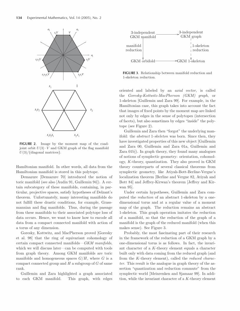
FIGURE 2. Image by the moment map of the coad-joint orbit U(3) · V and GKM graph of the flag manifoldU(3)/{diagonal matrices}.

Hamiltonian manifold. In other words, all data from theHamiltonian manifold is stored in this polytope.

Demazure [Demazure 70] introduced the notion oftoric manifold (see also [Audin 91, Guillemin 94]). A cer-tain subcategory of these manifolds, containing, in par-ticular, projective spaces, satisfy hypotheses of Delzant’stheorem. Unfortunately, many interesting manifolds donot fulfill these drastic conditions, for example, Grass-mannian and flag manifolds. Thus, during the passagefrom these manifolds to their associated polytope loss ofdata occurs. Hence, we want to know how to encode alldata from a compact connected manifold with action ofa torus of any dimension.

Goresky, Kottwitz, and MacPherson proved [Goreskyet al. 98] that the ring of equivariant cohomology ofcertain compact connected manifolds—GKM manifolds,which we will discuss later—can be computed with toolsfrom graph theory. Among GKM manifolds are toricmanifolds and homogeneous spaces G/H, where G is acompact connected group and H a subgroup of G of samerank.

Guillemin and Zara highlighted a graph associatedto each GKM manifold. This graph, with edges

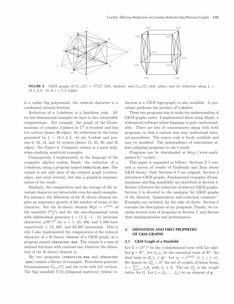
3-independentGKM manifold

��

manifoldreduction

��

3-independentGKM graph

1-skeletonreduction

��

GKM orbifold ��GKM 1-skeleton

FIGURE 3. Relationship between manifold reduction and1-skeleton reduction.

oriented and labeled by an axial vector, is calledthe Goresky-Kottwitz-MacPherson (GKM) graph, or1-skeleton [Guillemin and Zara 99]. For example, in theHamiltonian case, this graph takes into account the factthat images of fixed points by the moment map are linkednot only by edges in the sense of polytopes (intersectionof facets), but also sometimes by edges “inside” the poly-tope (see Figure 2).

Guillemin and Zara then “forgot” the underlying man-ifold: the abstract 1-skeleton was born. Since then, theyhave investigated properties of this new object [Guilleminand Zara 00, Guillemin and Zara 01a, Guillemin andZara 01b]). In graph theory, they found many analoguesof notions of symplectic geometry: orientation, cohomol-ogy, K-theory, quantization. They also proved in GKMtheory counterparts of several classical theorems fromsymplectic geometry, like Atiyah-Bott-Berline-Vergne’slocalization theorem [Berline and Vergne 82, Atiyah andBott 84] and Jeffrey-Kirwan’s theorem [Jeffrey and Kir-wan 95].

Under certain hypotheses, Guillemin and Zara com-puted the reduction of an abstract 1-skeleton by a one-dimensional torus and at a regular value of a momentmap of the graph. The reduction remains an abstract1-skeleton. This graph operation imitates the reductionof a manifold, so that the reduction of the graph of amanifold is the graph of the reduced manifold (when thismakes sense). See Figure 3.

Probably, the most fascinating part of their researchin the framework of the reduction of a GKM graph by aone-dimensional torus is as follows. In fact, the invari-ant character of a K-theory element equals a characterbuilt only with data coming from the reduced graph (andfrom the K-theory element), called the reduced charac-ter. This result is the analogue in graph theory of the as-sertion “quantization and reduction commute” from thesymplectic world [Meinrenken and Sjamaar 99]. In addi-tion, while the invariant character of a K-theory element

Cochet: Effective Reduction of Goresky-Kottwitz-MacPherson Graphs 135

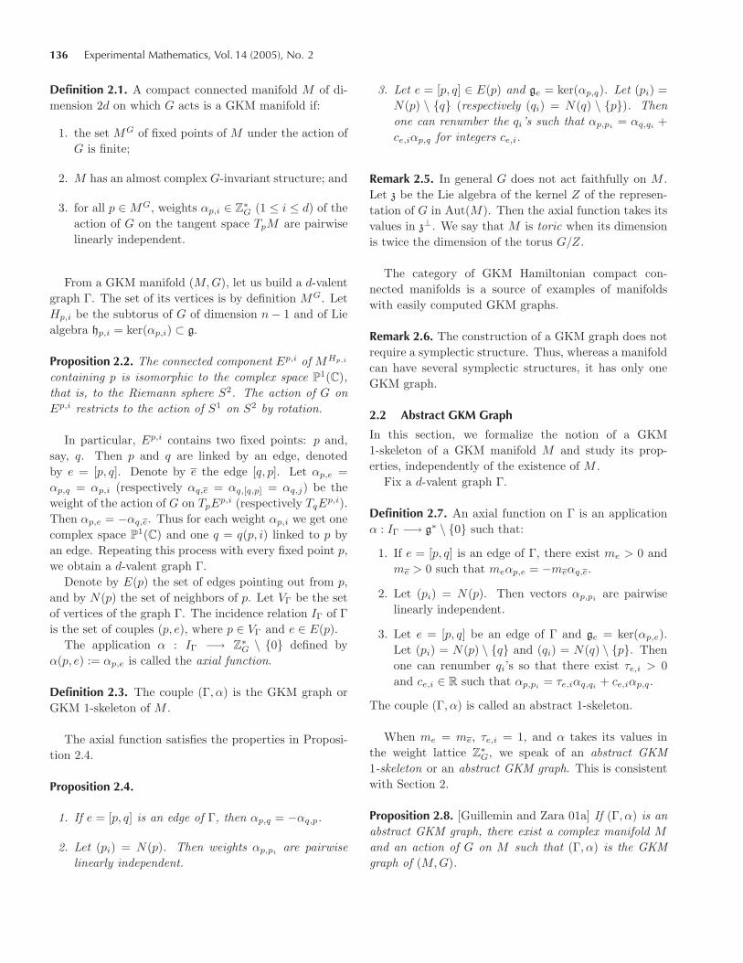
FIGURE 4. GKM graphs of G1,5(C) = P4(C) (left, dashed), and G2,5(C) (left, plain) and its reduction along ξ =

(0, 1, 2, 3,−6) at c = 7/2 (right).

is a rather big polynomial, the reduced character is acondensed rational fraction.

Reduction of a 1-skeleton is a fastidious task. Af-ter low-dimensional examples we have to face intractablecomputations. For example, the graph of the Grass-mannian of complex 2-planes in C

5 is 6-valent and hasten vertices (hence 30 edges). Its reductions by the torusgenerated by ξ = (0, 1, 2, 3,−6) are 5-valent and pos-sess 6, 10, 12, and 14 vertices (hence 15, 25, 30, and 35edges). See Figure 4. Computer science is a great help,when studying nontrivial examples.

Consequently, I implemented, in the language of thecomputer algebra system Maple, the reduction of a1-skeleton, using a program named reduction.mws. Theoutput is not only data of the reduced graph (vertices,edges, and axial vectors), but also a graphical represen-tation of the result.

Similarly, the computation and the storage of the in-variant character are intractable even for small examples.For instance, the dilatation of the K-theory element im-plies an impressive growth of the number of terms of thecharacter. For the K-theory element Θ(p) = e2iπθp ofthe manifold P

3(C) and for the one-dimensional toruswith infinitesimal generator ξ = (1, 2,−1,−2), invariantcharacters χ(Θn)H for n = 1, 10, 100, and 1, 000 haverespectively 1, 12, 867, and 83, 667 monomials. This iswhy I also implemented the computation of the reducedcharacter of a K-theory element of a GKM graph, in aprogram named character.mws. The output is a sum ofrational fractions with constant size whatever the dilata-tion of the K-theory element is.

My two programs (reduction.mws and character

.mws) contain a library of examples. Procedures generateGrassmannians Gk,n(C) and the cycle with 4N vertices.The flag manifold U(3)/{diagonal matrices} (whose re-

duction is a GKM hypergraph) is also available. A pro-cedure performs the product of 1-skeleta.

These two programs aim to make the understanding ofGKM graphs easier. I implemented them using Maple, awidespread software whose language is quite understand-able. There are lots of commentaries along with bothprograms, so that a curious user may understand inter-nal procedures. The source code is freely available andmay be modified. The independence of subroutines al-lows adapting programs to one’s needs.

Programs can be downloaded at http://www.math.jussieu.fr/∼cochet/.

This paper is organized as follows. Sections 2–5 con-tain a survey of results of Guillemin and Zara aboutGKM theory. Only Sections 6–7 are original. Section 2introduces GKM graphs. Fundamental examples (Grass-mannians and flag manifolds) are described in Section 3.Section 4 features the reduction of abstract GKM graphs.Section 5 is devoted to the analogue for GKM graphsof the theorem “quantization and reduction commute.”Examples are included, for the sake of clarity. Section 6contains the description of my programs. Finally, we ex-amine several tests of programs in Section 7, and discusstheir implementation and performances.

2. DEFINITION AND FIRST PROPERTIESOF GKM GRAPHS

2.1 GKM Graph of a Manifold

Let G = (S1)n be the n-dimensional torus with Lie alge-bra g = R

n. Let (ej)j be the canonical basis of Rn. Its

dual basis is (θj)j ⊂ g∗. Let uj = e2iπθj (1 ≤ j ≤ n).We denote by Z

∗G = Z

n the set of weights of linear formsλ =

∑nj=1 λjθj with λj ∈ Z. The set Z

∗G is the weight

lattice for G. Let ξ = (ξ1, . . . , ξn) be an element of g.


Definition 2.1. A compact connected manifold M of di-mension 2d on which G acts is a GKM manifold if:

1. the set MG of fixed points of M under the action ofG is finite;

2. M has an almost complex G-invariant structure; and

3. for all p ∈MG, weights αp,i ∈ Z∗G (1 ≤ i ≤ d) of the

action of G on the tangent space TpM are pairwiselinearly independent.

From a GKM manifold (M,G), let us build a d-valentgraph Γ. The set of its vertices is by definition MG. LetHp,i be the subtorus of G of dimension n− 1 and of Liealgebra hp,i = ker(αp,i) ⊂ g.

Proposition 2.2. The connected component Ep,i of MHp,i

containing p is isomorphic to the complex space P1(C),

that is, to the Riemann sphere S2. The action of G onEp,i restricts to the action of S1 on S2 by rotation.

In particular, Ep,i contains two fixed points: p and,say, q. Then p and q are linked by an edge, denotedby e = [p, q]. Denote by e the edge [q, p]. Let αp,e =αp,q = αp,i (respectively αq,e = αq,[q,p] = αq,j) be theweight of the action of G on TpE

p,i (respectively TqEp,i).

Then αp,e = −αq,e. Thus for each weight αp,i we get onecomplex space P

1(C) and one q = q(p, i) linked to p byan edge. Repeating this process with every fixed point p,we obtain a d-valent graph Γ.

Denote by E(p) the set of edges pointing out from p,and by N(p) the set of neighbors of p. Let VΓ be the setof vertices of the graph Γ. The incidence relation IΓ of Γis the set of couples (p, e), where p ∈ VΓ and e ∈ E(p).

The application α : IΓ −→ Z∗G \ {0} defined by

α(p, e) := αp,e is called the axial function.

Definition 2.3. The couple (Γ, α) is the GKM graph orGKM 1-skeleton of M .

The axial function satisfies the properties in Proposi-tion 2.4.

Proposition 2.4.

1. If e = [p, q] is an edge of Γ, then αp,q = −αq,p.

2. Let (pi) = N(p). Then weights αp,piare pairwise

linearly independent.

3. Let e = [p, q] ∈ E(p) and ge = ker(αp,q). Let (pi) =N(p) \ {q} (respectively (qi) = N(q) \ {p}). Thenone can renumber the qi’s such that αp,pi

= αq,qi+

ce,iαp,q for integers ce,i.

Remark 2.5. In general G does not act faithfully on M .Let z be the Lie algebra of the kernel Z of the represen-tation of G in Aut(M). Then the axial function takes itsvalues in z⊥. We say that M is toric when its dimensionis twice the dimension of the torus G/Z.

The category of GKM Hamiltonian compact con-nected manifolds is a source of examples of manifoldswith easily computed GKM graphs.

Remark 2.6. The construction of a GKM graph does notrequire a symplectic structure. Thus, whereas a manifoldcan have several symplectic structures, it has only oneGKM graph.

2.2 Abstract GKM Graph

In this section, we formalize the notion of a GKM1-skeleton of a GKM manifold M and study its prop-erties, independently of the existence of M .

Fix a d-valent graph Γ.

Definition 2.7. An axial function on Γ is an applicationα : IΓ −→ g∗ \ {0} such that:

1. If e = [p, q] is an edge of Γ, there exist me > 0 andme > 0 such that meαp,e = −meαq,e.

2. Let (pi) = N(p). Then vectors αp,piare pairwise

linearly independent.

3. Let e = [p, q] be an edge of Γ and ge = ker(αp,e).Let (pi) = N(p) \ {q} and (qi) = N(q) \ {p}. Thenone can renumber qi’s so that there exist τe,i > 0and ce,i ∈ R such that αp,pi

= τe,iαq,qi+ ce,iαp,q.

The couple (Γ, α) is called an abstract 1-skeleton.

When me = me, τe,i = 1, and α takes its values inthe weight lattice Z

∗G, we speak of an abstract GKM

1-skeleton or an abstract GKM graph. This is consistentwith Section 2.

Proposition 2.8. [Guillemin and Zara 01a] If (Γ, α) is anabstract GKM graph, there exist a complex manifold M

and an action of G on M such that (Γ, α) is the GKMgraph of (M,G).


Hence, it is acceptable to leave out the adjective “ab-stract,” when speaking of an “abstract GKM graph” oran “abstract GKM 1-skeleton.”

Remark 2.9. In Definition 2.7, I weakened both Defi-nition 2.1 and Proposition 2.4 by introducing me andτe,i, because, in general, the symplectic reduction of amanifold is an orbifold, and the reduction of an abstract1-skeleton (see Section 4), built as the analogue of thesymplectic reduction of a manifold, will be an abstract1-skeleton and not a GKM 1-skeleton.

Definition 2.10. The abstract 1-skeleton (Γ, α) isk-independent if for all vertices p and for all k-sets ofneighbors {q1, . . . , qk} of p, the family {αp,q1 , . . . , αp,qk

}is linearly independent.

3. CLASSICAL EXAMPLES OF GKM MANIFOLDSAND GRAPHS

3.1 The Grassmannian Gk,n(C)

The Grassmannian M = Gk,n(C) of complex k-planesin C

n is equipped with the action of the complex torusT = (S1)n deduced from the natural action on C

n.This manifold has complex dimension k(n − k),

whereas the quotient of the torus by the kernel of theaction is (n − 1)-dimensional. Hence, if k is differentfrom 1 and n − 1, conditions of Delzant’s theorem arenot fulfilled. Hence, the image of a moment map doesnot contain all data from the manifold.

Vertices of the GKM graph of Gk,n(C) are in one-to-one correspondence with k-subsets S of {1, . . . , n}. Thevertex pS corresponds to the k-dimensional space gener-ated by ej (j ∈ S). Two vertices pS and pS′ are adjacentif and only if S ∩ S′ has k − 1 elements. Moreover theaxial function is αpS ,pS′ =

∑i∈S′ θi −

∑j∈S θj .

This graph has(

n

k

)vertices, each of them linked with

k(n− k) adjacent vertices. Consequently, there are

k(n− k)2

(n

k

)=

n(n− 1)2

(n− 2k − 1

)

edges. We will often write pS = S.The projective space P

n(C) = G1,n+1(C) is equippedwith the effective action of the n-dimensional torus(S1)n+1/(eiθ, . . . , eiθ). The Fubini-Study form endowsit with a Hamiltonian structure with moment mapφ([z])(X) = −i〈X(z), z〉/|z|2 (z ∈ C

n+1, X ∈ g). Thisspace satisfies the hypotheses of Delzant’s theorem, thusthe image of the moment map characterizes this space.

1

��

��

��

��

� 2

��

��

��

��

�12

��

��

�� 13

��

��

��

14

��

��

�� 23

4 3 24

��34

��

FIGURE 5. GKM graphs of P3(C) and G2,4(C) (axial

function omitted).

idα1

�� α2

α3

s1

α3

α2

s2

α3

α1

��

s2s1

α2�� s1s2

α1

w0

FIGURE 6. GKM graph of the flag manifold GL(3, C)/B.

3.2 The Flag Manifold U(n)/{diagonal matrices}Let K = U(n) be the group of n × n unitary matricesand D be the subgroup of K of diagonal unitary matri-ces. Denote by M = U(n)/D � GL(n, C)/B the flagmanifold of GL(n, C), where B is the Borel subgroupof GL(n, C) of invertible upper triangular matrices. Thismanifold does not fulfill the hypotheses of Delzant’s theo-rem, hence the GKM graph is valuable for characterizingthis space.

The GKM graph of the flag manifold GL(n, C)/B is,in fact, the Cayley graph associated to the permutationgroup Sn. Vertices of Γ are in one-to-one correspondencewith permutations over {1, . . . , n}. Two vertices σ, σ′ arelinked by an edge if and only if there exists a transposi-tion ti,j = (i j) such that σ′ = σti,j . Moreover ασ,σti,j

equals θj − θi if σ(j) > σ(i), else θi − θj .For example, let α1 = θ2 − θ1, α2 = θ3 − θ2, and

α3 = α1 +α2. Then Figure 6 represents the GKM graphof GL(3, C)/B.

4. REDUCTION OF A 3-INDEPENDENT ABSTRACT1-SKELETON

Let (Γ, α) be a d-valent abstract 1-skeleton. Here we as-sume that (Γ, α) is 3-independent (see Definition 2.10).


When (Γ, α) is not 3-independent we can still com-pute a reduction, but the result will be a hypergraph(see [Guillemin and Zara 00]). Although my programscan handle this case, I will not describe this similar the-ory here.

Fix a one-dimensional subtorus H of G with infinitesi-mal generator ξ ∈ g lying in no ker(αp,e) (where e = [p, q]runs over the set of edges). This vector ξ gives rise to agraph orientation oξ for (Γ, α), by saying that the edge[p, q] satisfies p < q if and only if αp,e(ξ) < 0.

Assume that, for any codimension 2 subspace h of g

and for any divalent subgraph Γh that has edges [p, q]such that αp,q ∈ h⊥, each connected component Γ0 ofΓh has exactly one maximum and one minimum (for theorientation oξ). We say that Γ is strongly acyclic.

Let f be a cohomology element of (Γ, α), that is f :Γ −→ g∗ such that f(q) − f(p) = λeαp,e for all edgese = [p, q]. We assume that f is symplectic, that is, λe > 0for all e. The application φ = φf,ξ : VΓ −→ R defined byφ(p) = 〈f(p), ξ〉 satisfies φ(p)−φ(q)

αq,e(ξ) > 0 for all e = [p, q];we then say that φ is an H-moment for (Γ, α). Fix aregular value c for φ.

Let us build the reduced 1-skeleton, a graph Γc withvalence d − 1 that will be an abstract 1-skeleton withaxial function vanishing on ξ. This corresponds to thefact that the reduction of a 2d-dimensional manifold M

is a 2(d−1)-dimensional orbifold endowed with the actionof G/H.

Vertices SΓcof Γc are oriented edges e = [p, q] such

that φ(p) < c < φ(q). For such an edge e = [p, q], denoteby qi all (d−1) neighbors of p other than q. Fix an indexi. Let hi be the intersection of kernels of linear forms αp,q

and αp,qi. The connected component Γ0 of Γhi

containingp, q, and qi is divalent, thanks to 3-independence. Byhypothesis (Γ, α) is strongly acyclic, hence there exist inΓ0 exactly two edges cut by c, namely e and another one,denoted by e′ = [p′, q′]. We then link vertices [p, q] and

FIGURE 7. Reduction of an abstract 1-skeleton.

[p′, q′] by an edge in the reduction. See Figure 7. Theaxial function on the edge [e, e′] of Γc is

αce,e′ = αp,qi

− αp,qi(ξ)

αp,q(ξ)αp,q. (4–1)

Notice that this is indeed a linear form vanishing on ξ.

Theorem 4.1. [Guillemin and Zara 01a] The graph(Γc, αc) is an abstract 1-skeleton with valence (d − 1).If (Γ, α) is k-independent, then (Γc, αc) is (k − 1)-independent.

When the abstract 1-skeleton (Γ, α) comes from a sym-plectic GKM manifold with Hamiltonian action, the re-duction of (Γ, α) coincides with the GKM graph of thereduced manifold: Γ(M)c = Γ(Mc).

Remark 4.2. The reduction does not change when c runsover a connected component of the set of regular points.Note also, that when we add a vector λ0 ∈ g∗ to f ,all data are translated. Consequently, one can alwaysconsider the reduction at c = 0.

Example 4.3. (Reductions of P4(C).) Let H be the one-

dimensional subtorus of (S1)4 with infinitesimal genera-tor ξ = (4, 3, 2, 1,−10). Since the GKM graph of P

4(C) is4-independent, its reductions are 3-independent abstractGKM 1-skeleta. Choose f(i) = θi as a symplectic coho-mology element. Critical values for φ = φf,ξ are 4, 3, 2,1, and −10. In fact, we can restrict ourselves to reduc-tions at c = 7/2, 5/2, 3/2, and 0. Reductions at c = 7/2and 0 are the same as at c = 5/2 and 3/2. See Figures 8and 9.

Example 4.4. (Reductions of GL(3, C)/B.) Since theGKM graph of GL(3, C)/B is not 3-independent, its re-ductions are not graphs but hypergraphs. Let H be gen-erated by ξ = (2, 1,−3). Let α1 = θ2 − θ1, α2 = θ3 − θ2,and α3 = α1 + α2. Choose as a symplectic cohomologyelement the function f defined by

f(id) = −(α1 + α2),f(s1) = −α2,

f(s2s1) = α1,f(w0) = (α1 + α2),f(s2) = −α1,

f(s1s2) = α2.

Critical values for φ = φf,ξ are ±5, ±4, and ±1. We canrestrict ourselves to reductions at c = ±3/2, ±9/2, and0. Reductions at c = ±3/2 are the same as at c = ±9/2.


FIGURE 8. Reduction of P4(C) along ξ = (4, 3, 2, 1,−10) and at c = 7/2.

FIGURE 9. Reduction of P4(C) along ξ = (4, 3, 2, 1,−10) and at c = 5/2.

FIGURE 10. Reductions of GL(3, C)/B by ξ = (2, 1,−3) at c = 3/2, c = 0 and c = 9/2.

In every case, the reduced graph has a unique hyperedgelinking all vertices. See Figure 10.

5. QUANTIZATION AND REDUCTION COMMUTE

This section deals with the analogue of “quantizationand reduction commute” for GKM graphs, as proved byGuillemin and Zara [Guillemin and Zara 01b] in the caseof reduction by a one-dimensional torus.

Let (Γ, α) be a d-valent abstract 1-skeleton. Fix a one-dimensional subtorus H of G with infinitesimal generatorξ ∈ g lying in no ker(αp,e).

Let f be a cohomology element for (Γ, α) with valuesin Z

∗G. The application Θ(p) = e2iπf(p) is called a K-

theory element for (Γ, α). The character of Θ is thendefined by

χ(Θ) =∑p∈VΓ

Θ(p)∏e∈Ep

(1− e2iπαp,e). (5–1)

In fact, the character χ(Θ) has no pole [Guillemin andZara 01b].

Assume that the abstract 1-skeleton is a GKM graph(that is, coming from a manifold) and that f is symplectic(λe > 0 for all e). Let φ(p) = 〈f(p), ξ〉 be the H-moment.Fix a regular value c for φ.

Guillemin and Zara proved that the invariant charac-ter χ(Θ)H (defined as the part of χ(Θ) invariant underthe action of H) can be expressed in terms of a GKMgraph and Θ, under the condensed form of a sum of ra-tional fractions. This more precisely expressed in Theo-rem 5.1.


Theorem 5.1. [Guillemin and Zara 01b] The reduced char-acter χc(Θ) is, by definition,

∑[p,q]∈Γc

1|αp,q(ξ)|×

∑ζαp,q(ξ)=1

ζ〈f(p),ξ〉e2iπ�

f(p)− 〈f(p),ξ〉αp,q(ξ) αp,q

�

∏r∈N(p)\{q}

(1−ζαp,r(ξ)e

2iπ�

αp,r−αp,r(ξ)αp,q(ξ) αp,q

�) .

Then the invariant character equals the reduced characterχc=0(Θ).

Remark 5.2. In the case of the reduction of a Hamil-tonian manifold, Meinrenken and Sjamaar [Meinrenkenand Sjamaar 99] proved the equality χc(Θ) = χ(Θ)H ata regular value c close to zero. Although Mc and (Γc, αc)change when c crosses the critical value 0, the characterχc(Θ) remains unchanged. This result is still true in theframework of examples that we will discuss in Section 6.Hence in these examples, when 0 is not regular, we com-pute the reduced character at the regular value c = 1/10close enough to 0.

Remark 5.3. Theorem 5.1 has two consequences. First,we have a condensed expression (sum of rational frac-tions) of χ(Θ)H . In fact, when (Γ, α) comes from aHamiltonian manifold M , the character of Q(M)H ishuge. Second, the formula of Guillemin and Zara involvessums over roots of unity. When these roots are reason-able, computation is possible and does not explode when,for example, one dilates Θ.

Example 5.4. (Case of P3(C).) Let H be the

one-dimensional torus generated by ξ = (1, 2,−1,−2).Choose f�(p) = θp (p = 1, . . . , 4) with ∈ N

∗ and letΘ�(p) = e2iπf�(p). Let uj = e2iπθj (j = 1, . . . , 4). Hencethe invariant character is χ(Θ�)H =

∑u�1

1 u�22 u�3

3 u�44 ,

where the sum is over the set of integers (1, 2, 3, 4) ∈N

4 such that 1 + 2 + 3 + 4 = and 1 +22 = 3 +24.The result is a polynomial in uj with the number ofmonomials quadratic in . For example χ(Θ500)H has21001 monomials spreading over 93 pages.

On the other hand, one can check that Theorem 5.1leads to a condensed formula in which size does not varywhen grows. For example, χ0(Θ6m) equals

u2m+12 u4m+2

3 (u2u33 + u2

1u3u4 + u1u2u24)

(u22u3 − u3

1)(u43 − u2u3

4)

+u3m+1

2 u3m+14 (u3

2u34+u1u2u3u4+u2

1+u21u2u

23u4+u3

1u33)

(u32u4 − u4

1)(u2u34 − u4

3)

+u4m+2

1 u2m+14 (u3

1u4 + u22u3u4 + u1u2u

23)

(u41 − u3

2u4)(u1u24 − u3

3)

+u3m+2

1 u3m+23 (u1u3 + u2u4)

(u31 − u2

2u3)(u33 − u1u2

4).

Formulas for χ0(Θ6m+k) (1 ≤ k ≤ 5) are similar.

Remark 5.5. A direct computation of the invariant char-acter leads to the enumeration of indices satisfying linearconditions of the form

∑j ajj = T () (for an affine op-

erator T ) intractable problem when grows.

Remark 5.6. In the case of toric manifolds, the re-duced manifold is still toric. Brion’s formulas [Brionand Vergne 97, Barvinok 02] have been recently imple-mented in polynomial time with Barvinok’s algorithm bythe LattE team [De Loera et al. 04].

6. PROGRAMS

This section describes my programs reduction.mws andcharacter.mws, computing respectively the reduction ofan abstract 1-skeleton and the reduced character of aK-theory element of a GKM 1-skeleton. Recall thatgraph reduction needs an abstract 1-skeleton (Γ, α) (plusother hypotheses). It returns a graph (more precisely anabstract 1-skeleton) if (Γ, α) is 3-independent, otherwiseit returns a hypergraph. On the other hand, characterreduction needs a GKM 1-skeleton but is independent ofthe notion of 3-independence.

6.1 Data Storage and Program Handling

Fix a numbering p1, . . . , pN of vertices of the abstract1-skeleton. The set of vertices is represented by the listS = (p1, . . . , pN ). Edges and axial function are storedin the N ×N matrix A such that ai,j = αpi,pj

if pi andpj are adjacent, else ai,j = 0. The matrix A is the gen-eralized adjacence matrix of (Γ, α) (for this numbering).This matrix allows an efficient check for adjacence, cy-cles, connected components, etc.

Hence, an abstract 1-skeleton is represented by thematrix A and the list S.

The cohomology element f is encoded by the listF = (f(p1), . . . , f(pN )). Vectors and linear forms arerepresented in the canonical basis of R

n; hence, the eval-uation of a form on a vector corresponds to a scalarproduct.

Example 6.1. Let us fix the numbering p1 = 1, p2 = 2,p3 = 3 of vertices of the GKM graph of P

2(C); hence,


S = (1, 2, 3). Since αpi,pj= θj − θi, the generalized

adjacence matrix is

0 (−1, 1, 0) (−1, 0, 1)

(1,−1, 0) 0 (0,−1, 1)(1, 0,−1) (0, 1,−1) 0

.

The cohomology element f(p) = θi is represented by F =((1, 0, 0), (0, 1, 0), (0, 0, 1)). Suitable ξ and regular valuec are, for example, (2, 1,−3) and 3/2.

My two programs are easy to use: the user only pro-vides the 1-skeleton and reduction or character data, un-der the form S, A, F , ξ, c. This can be done eithermanually, or with procedures generating classical exam-ples (Grassmannian, GL(3, C)/B, cycle with 4N vertices,product of graphs). For example, consider the reduc-tion of G2,4(C) by the torus of infinitesimal generatorξ = (3, 2, 1,−6), at the regular value c = 0. Then thecommand lines building data associated to this reductionas well as the cohomology element f(p) = 5θp inducingthe moment map are described below.

S := Sgrass(2,4);A := Agrass(2,4);F := Fgrass(2,4,5);xi := [3,2,1,-6];c := 0;

Command lines for computing vertices, cohomologyelement, and generalized adjacence matrix of the reducedgraph are described below. The last line gives a graphicalrepresentation of the graph.

Sred := VerticesRedGraph(S,F,A,xi,c);Ared := Reduction(S,F,A,xi,c);Fred := CohomologyRedGraph(S,F,A,xi,c);PrintGraph(Ared);

On the other hand, the command line for the reducedcharacter is

P := CharacterRed(S,F,A,xi,c);

Both programs (for reduction and character compu-tation) contain internal checks pointing out to the userthe possible failure of any condition on input data (seeProposition 2.4, Definition 2.7, Sections 4 and 5).

6.2 Reduction of a 3-Independent Abstract GKM1-Skeleton

The first step of the program reduction.mws is to find allvertices of the reduced graph, that is, all edges e = [p, q]

with φ(p) < c < φ(q). Let us fix such an edge e = [p, q]and let r be a neighbor of p different from q.

Three-independence implies that there exists a uniqueneighbor s of r other than p such that the tripleof vectors {αq,p, αp,r, αr,s} has rank 2 (see Fig-ure 7). Finding this s is performed by the proce-dure NeighborDimTwo(A,q,p,r); its implementation isstraightforward.

The algorithm computing the reduction of a3-independent abstract 1-skeleton is:

For all vertex e = [p, q] of the reduced 1-skeletonfor all neighbor r of p other than q

compute the reduced axial functionfind the only neighbor s of r other than p. . .. . . such that {αq,p, αp,r, αr,s} has rank 2repeat

if [r, s] is cut by c

then link [p, q] and [r, s] in the reduced. . .. . . 1-skeleton

quit the “repeat” loopelse q ←− p

p←− r

r ←− s

end ifend of “repeat”

end of loop over neighbors of p

end of loop over vertices of the reduced graph

Note that strong acyclicity ensures us that the pro-gram will never be trapped in an infinite “repeat” loop.

6.3 Computing the Invariant Character as a Sum ofRational Fractions

The difficult part of character.mws is not implement-ing formulas, but finding an efficient way to do it. Araw procedure leads to computations that explode, evenfor small examples. More precisely, we need to computesums appearing in Theorem 5.1;

S(m; k, k1, . . . , kd) =m∑

�=1

ζ�k

(1− ζ�k1U1) · · · (1− ζ�kdUd),

where ζ is the mth root of unity e2iπm and Uj are indeter-

minates. Using a formal series development, one easilyobtains an expression that may be used (see [Zagier 73]);

S(m; k, k1, . . . , kd) =

∑m−1s1,...,sd=0 as1,...,sd

Us11 · · ·Usd

d

(1− Um1 ) · · · (1− Um

d ),


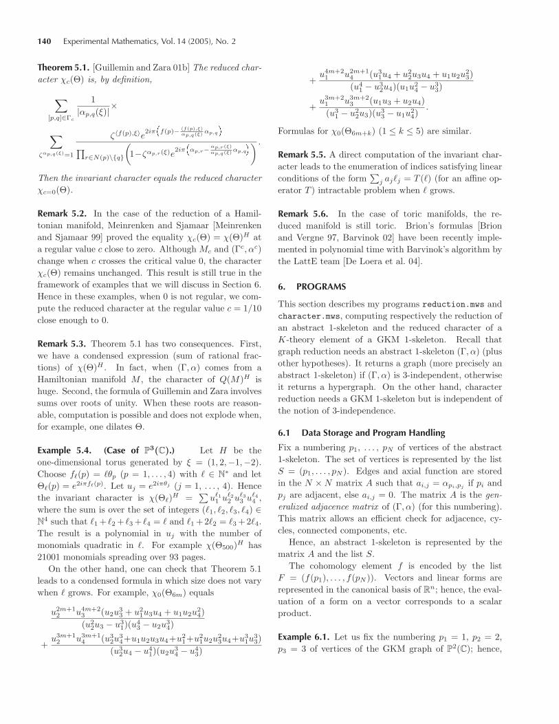
Graph of the manifold Dim. effective torus Valence Number of vertices

P2(C) 2 2 3

GL(3, C)/B 2 3 6

G2,4(C) 3 4 6

P5(C) 5 5 6

G2,5(C) 4 6 10

P4(C) × GL(3, C)/B 6 7 30

P8(C) 8 8 9

G3,6(C) 5 9 20

G2,4(C) × G2,5(C) 7 10 60

P20(C) 20 20 21

G5,10(C) 9 25 252

G6,13(C) 12 42 1716

TABLE 1. GKM graphs of classical manifolds.

where as1,...,sdequals n when m divides k + k1s1 + · · ·+

kdsd, else 0.Marc A. A. van Leeuwen has performed an efficient re-

cursive implementation of this formula, in the procedureSumRootUnit(k,L,X,U,m). Here L is the list of constantskj and X is an intermediary variable. The algorithm ofthe procedure is:

let d be the cardinal of Llet recur(level,s) be a local procedure defined by

if level is strictly greater than d

then return Xs mod m

else return the sum for t = 0, . . . , m− 1 of. . .. . . U t

level * recur(level+1,s-t*Lniv)

end of local procedurelet R be the coefficient of the polynomial. . .. . . recur(1,0) in X of degree k mod m

return m×R divided by the product of (1− Ukj),. . .

. . . with j ranging from 1 to d.

This procedure returns the sum of |Γ0| rational frac-tions. The dilatation of the cohomology element by a fac-tor —even of the order of billion—does not cost moretime or memory. Only a monomial factor before eachfraction grows, while the result under polynomial formexplodes (see Example 5.4).

7. TEST OF PROGRAMS

Let me begin with several general remarks.I stress that I rewrote Maple procedures on vectors:

addition, multiplication by a constant, scalar product,test of colinearity, rank of three vectors, etc. This greatlyincreased the speed of the programs. Moreover, usinglists instead of vectors has gained a lot of time. Finally,

encoding the null vector (corresponding to two nonad-jacent vertices) by the integer 0 in the generalized adja-cence matrix allowed a fast test of edges. More generally,great care towards efficiency was taken during the imple-mentation.

Here, I describe tests on classical examples of GKMgraphs coming from Grassmannians, from the flag man-ifold GL(3, C)/B, and their products. In Table 1, onecan find for several classical manifolds: dimension of ef-fective torus acting, valence, and number of vertices ofthe graph.

For the Grassmannian Gn,k(C), the cohomology el-ement is f(pS) =

∑s∈S θs (see Example 4.3). For

the flag manifold GL(3, C)/B the cohomology elementis described in Example 4.4. Denote by ξr the vector(r−1, . . . , 1,−r(r−1)/2) ∈ C

r. In my examples I alwaysreduced at the regular value c = 1/10 (see Remark 5.2).Recall that the valence d of the GKM 1-skeleton equalsthe dimension of the underlying manifold. Moreover, thereduced graph has valence d− 1.

Tests were performed on standard 1.13-GHz computer,running Maple 9. I checked retro-compatibility down toMaple Vr5.

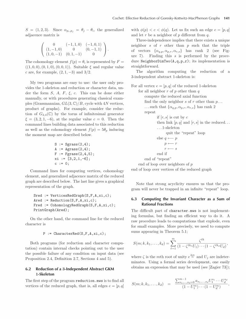
Note that for graph reduction most of the computa-tion time is spent checking colinearity of two vectors andchecking the rank of a system of three vectors. Improv-ing, even slightly, the speed of these two tasks would leadto a substantial time savings. Nevertheless, the reductionof 25-valent graphs with hundreds of vertices is alreadydone in a very competitive time. See Table 2.

Now come remarks on character reduction. The proce-dure SumRootUnit(k,L,X,U,m), computing recursivelysums of roots of unity and described in Section 6.3, isreally efficient. Its two main parameters (directly influ-encing computation time) are the valence of the graph


Manifold Generator ξ Nb. of vertices Nb. of (hyper)edges Computationto be reduced of H of reduced graph of reduced graph time

P2(C) ξ3 2 1 < 0.1 sec

GL(3, C)/B (1, 0,−1) 5 1 < 0.1 sec

G2,4(C) ξ4 6 9 < 0.1 sec

P5(C) ξ6 5 10 < 0.1 sec

P5(C) (3, 2, . . . ,−3) 9 18 < 0.1 sec

G2,5(C) (3, 2, 1, 0,−6) 12 30 0.1 sec

P4 × GL(3)/B ξ8 20 45 11.6 sec

P8(C) (4, 3, . . . ,−4) 20 70 0.2 sec

G3,6(C) (3, 2, . . . ,−3) 37 148 0.4 sec

G2,4 × G2,5 ξ9 72 324 9.8 sec

P20(C) ξ21 20 190 2.2 sec

G5,10(C) ξ10 630 7560 84.7 sec

G6,13(C) ξ13 5544 113652 8113.0 sec

TABLE 2. Reduction of GKM graphs of classical manifolds.

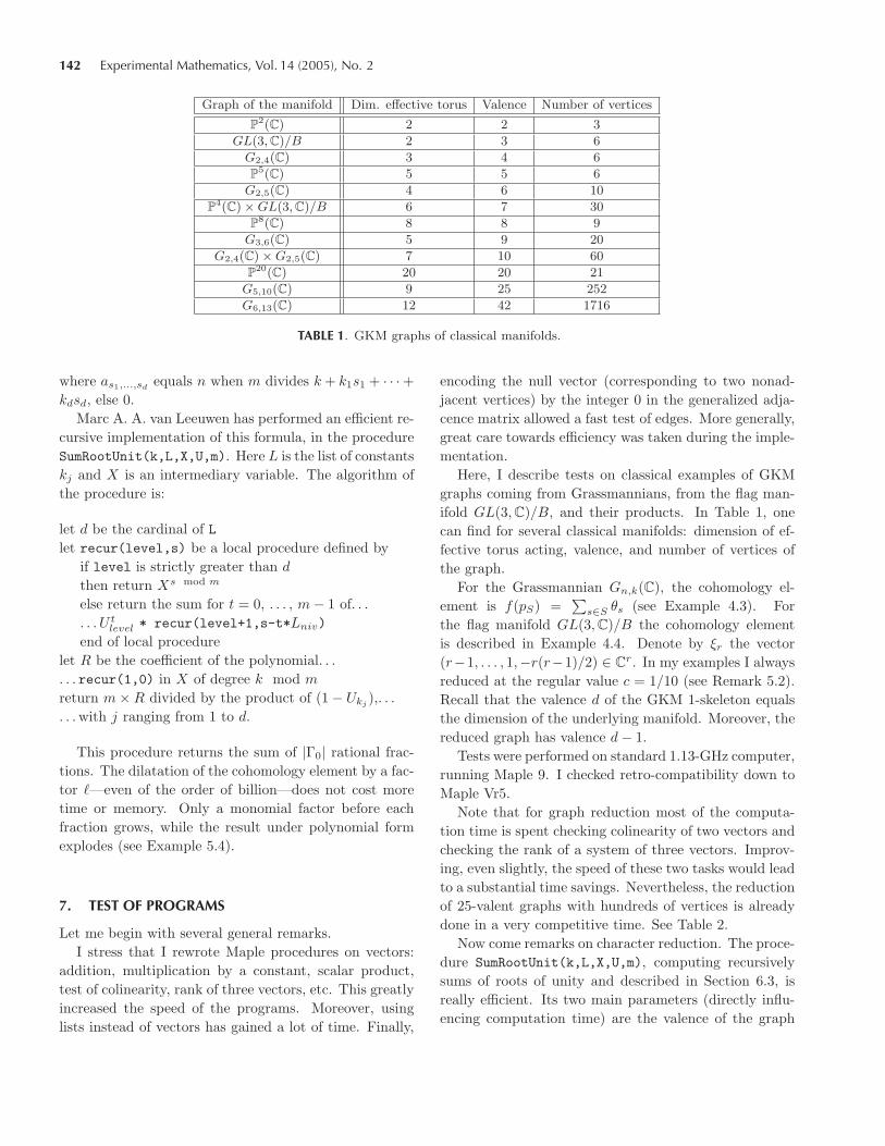
Manifold Generator ξ Nb. of vertices Order of Computationto be reduced of H of reduced graph roots of unity time

P2(C) ξ3 2 4 and 5 < 0.1 sec

GL(3, C)/B (1, 0,−1) 5 1 and 2 < 0.1 sec

G2,4(C) ξ4 6 7 to 9 0.1 sec

P5(C) ξ6 5 16 to 20 22.0 sec

P5(C) (3, 2, . . . ,−3) 9 2 to 6 0.2 sec

G2,5(C) (3, 2, 1, 0,−6) 12 6 to 9 16.9 sec

P8(C) (4, 3, . . . ,−4) 20 1 to 8 743.0 sec

G3,6(C) (3, 2, . . . ,−3) 37 1 to 6 891.4 sec

TABLE 3. Computation of the reduced character of a K-theory element of classical manifolds.

and the values αp,q(ξ) involved in Theorem 5.1. On onehand, the valence changes the depth of recursivity. Onthe other hand, sums are over roots of unity of orderαp,q(ξ), where [p, q] runs over all vertices of the reducedgraph.

However, for every reduced character computation, weneed to call this procedure for each vertex of the reducedgraph. Each call to the procedure gives a rational fractionappearing in the result. Hence, computing a reducedcharacter is quite expensive when the reduced graph hasmany vertices.

For a fixed manifold, it is interesting to see what hap-pens when we change the torus H. This influences thenumber of sums of roots of unity that need to be evalu-ated and the nature of the roots of unity. See Table 3 forexamples of computations of the reduced character of aK-theory element of a GKM graph.

ACKNOWLEDGMENTS

The author thanks the referee for his/her careful work andjudicious remarks.

REFERENCES

[Atiyah and Bott 84] M. F. Atiyah and R. Bott. “The Mo-ment Map and Equivariant Cohomology.” Topology 23:1(1984), 1–28.

[Audin 91] Michele Audin. The Topology of Torus Actions onSymplectic Manifolds. Basel: Birkhauser Verlag, 1991.

[Barvinok 02] Alexander Barvinok. A Course in Convexity,Graduate Studies in Mathematics, 54. Providence, RI:American Mathematical Society, 2002.

[Berline and Vergne 82] Nicole Berline and Michele Vergne.“Classes caracteristiques equivariantes. Formule de lo-calisation en cohomologie equivariante.” C. R. Acad. Sci.Paris Ser. I Math. 295:9 (1982), 539–541.

[Brion and Vergne 97] Michel Brion and Michele Vergne.“Residue Formulae, Vector Partition Functions and Lat-tice Points in Rational Polytopes.” J. Amer. Math. Soc.10:4 (1997), 797–833.

[De Loera et al. 04] Jesus A. De Loera, Raymond Hemmecke,Jeremiah Tauzer, and Ruriko Yoshida. “Effective LatticePoint Counting in Rational Convex Polytopes.” J. Sym-bolic Comput. 38:4 (2004), 1273–1302.


[Delzant 88] Thomas Delzant. “Hamiltoniens periodiques etimages convexes de l’application moment.” Bull. Soc.Math. France 116:3 (1988), 315–339.

[Demazure 70] Michel Demazure. “Sous-groupes algebriquesde rang maximum du groupe de Cremona.” Ann. Sci.Ecole Norm. Sup.(4) 3 (1970), 507–588.

[Goresky et al. 98] Mark Goresky, Robert Kottwitz, andRobert MacPherson. “Equivariant Cohomology, KoszulDuality, and the Localization Theorem.” Invent. Math.131:1 (1998), 25–83.

[Guillemin 94] Victor Guillemin. Moment Maps and Combi-natorial Invariants of Hamiltonian T n-spaces, Progressin Mathematics, 122. Boston, MA: Birkhauser BostonInc., 1994.

[Guillemin and Zara 99] Victor Guillemin and Catalin Zara.“Equivariant de Rham Theory and Graphs.” Asian J.Math. 3:1 (1999), 49–76.

[Guillemin and Zara 00] Victor Guillemin and Catalin Zara.“Morse Theory on Graphs.” math.CO/0007161, 2000.

[Guillemin and Zara 01a] Victor Guillemin and Catalin Zara.“1-Skeleta, Betti Numbers, and Equivariant Cohomol-ogy.” Duke Math. J. 107:2 (2001), 283–349.

[Guillemin and Zara 01b] Victor Guillemin and Catalin Zara.“G-Actions on Graphs.” Internat. Math. Res. Notices2001:10 (2001), 519–542.

[Jeffrey and Kirwan 95] Lisa C. Jeffrey and Frances C. Kir-wan. “Localization for Nonabelian Group Actions.”Topology 34:2 (1995), 291–327.

[Meinrenken and Sjamaar 99] Eckhard Meinrenken andReyer Sjamaar. “Singular Reduction and Quantization.”Topology 38:4 (1999), 699–762.

[Zagier 73] Don Zagier. “Higher Dimensional DedekindSums.” Math. Ann. 202 (1973), 149–172.

Charles Cochet, Institut de Mathematiques de Jussieu, Universite Paris 7, UFR de mathematiques, UMR 7586, case 7012,2 place Jussieu, 75251 Paris cedex 05, France ([email protected]) http://www.math.jussieu.fr/∼cochet/

Received April 29, 2004; accepted September 23, 2004.

Documents

Effective Reduction of Goresky-Kottwitz-MacPherson Graphsemis.maths.adelaide.edu.au/journals/EM/expmath/volumes/14/14.2/...Effective Reduction of Goresky-Kottwitz-MacPherson Graphs