Effective Gene Expression Annotation Approaches for

Mouse Brain Images

by

Xinlin Zhao

A Thesis Presented in Partial Fulfillment

of the Requirements for the Degree

Master of Science

Approved January 2016 by the

Graduate Supervisory Committee:

Jieping Ye, Co-Chair

Yalin Wang, Co-Chair

Baoxin Li

ARIZONA STATE UNIVERSITY

May 2016

i

ABSTRACT

Understanding the complexity of temporal and spatial characteristics of gene

expression over brain development is one of the crucial research topics in neuroscience.

An accurate description of the locations and expression status of relative genes requires

extensive experiment resources. The Allen Developing Mouse Brain Atlas provides a

large number of in situ hybridization (ISH) images of gene expression over seven

different mouse brain developmental stages. Studying mouse brain models helps us

understand the gene expressions in human brains. This atlas collects about thousands of

genes and now they are manually annotated by biologists. Due to the high labor cost of

manual annotation, investigating an efficient approach to perform automated gene

expression annotation on mouse brain images becomes necessary. In this thesis, a novel

efficient approach based on machine learning framework is proposed. Features are

extracted from raw brain images, and both binary classification and multi-class

classification models are built with some supervised learning methods. To generate

features, one of the most adopted methods in current research effort is to apply the bag-

of-words (BoW) algorithm. However, both the efficiency and the accuracy of BoW are

not outstanding when dealing with large-scale data. Thus, an augmented sparse coding

method, which is called Stochastic Coordinate Coding, is adopted to generate high-level

features in this thesis. In addition, a new multi-label classification model is proposed in

this thesis. Label hierarchy is built based on the given brain ontology structure.

Experiments have been conducted on the atlas and the results show that this approach is

efficient and classifies the images with a relatively higher accuracy.

ii

This thesis is dedicated to my mom for her endless love and support.

iii

ACKNOWLEDGMENTS

I would like to thank all the professors and students who helped or taught me during my

two years of graduate study at Arizona State University. The completion of this thesis is

impossible without them.

I would like to thank Dr. Jieping Ye for his help in academia and research and for

providing such an interesting and challenging problem to me. Without his help and

support, I would not have been able to complete my Master’s degree. I would like to

thank Dr. Yalin Wang for being my co-chair and give me so many valuable advisements

about my research and thesis. I also would like to thank Dr. Baoxin Li for being a part of

my thesis committee and giving me instructions on my thesis.

Thanks to Tao Yang for giving me many helpful suggestions during the process

of experiment design and performance evaluation. I would like to thank Qian Sun for her

review and helpful suggestions to my thesis. In addition, I would like to thank everyone

in our lab, Shuo Xiang, Qingyang Li, Sen Yang, Yashu Liu, Zheng Wang, Binbin Lin,

Kefei Liu, Pinghua Gong and Jie Wang, for your care and nice help throughout my life

and education in America.

Finally yet importantly, I would like to thank my parents, without their love and

support, I would not have been able to complete a graduation education.

iv

TABLE OF CONTENTS

1. Page

LIST OF TABLES ............................................................................................................ vii

LIST OF FIGURES ......................................................................................................... viii

CHAPTER

1. BACKGROUND AND INTRODUCTION ............................................................ 1

1.1 Background .......................................................................................................... 1

1.2 Challenges ............................................................................................................ 3

1.2.1 Large Data Size Challenge ............................................................................3

1.2.2 Imbalanced Data Challenge ...........................................................................4

1.2.3 Multi-class Challenge ....................................................................................5

1.2.4 Multi-label Challenge ....................................................................................5

1.3 Problem Setup ...................................................................................................... 6

1.4 Methods and Approaches ..................................................................................... 6

1.5 Thesis Organization.............................................................................................. 8

2. DATASETS AND PREPROCESSING ................................................................... 9

2.1 Data ...................................................................................................................... 9

2.2 Brain Ontology ................................................................................................... 10

2.2.1 Ontology Structure .......................................................................................10

2.2.2 Propagation Strategy ....................................................................................11

v

CHAPTER Page

2.3 Preprocessing ..................................................................................................... 13

2.3.1 Imbalanced Data ..........................................................................................13

2.3.2 Random Undersampling ..............................................................................14

2.4 Summary ............................................................................................................ 17

3. FEATURE SELECTION FRAMEWORK ............................................................ 18

3.1 Learn from Feature Selection ............................................................................. 18

3.2 Image-level Feature Extraction .......................................................................... 19

3.3 High-level Feature Extraction ............................................................................ 20

3.4 Gene-level Feature Extraction ............................................................................ 22

3.5 Summary ............................................................................................................ 23

4. CLASSIFICATION METHODS ........................................................................... 24

4.1 SVM ................................................................................................................... 24

4.2 Binary-class Sparse Logistic Regression ........................................................... 25

4.3 Multi-task Sparse Logistic Regression ............................................................... 25

4.4 Majority Voting .................................................................................................. 26

4.5 Structure-based Multi-label Annotation over Brain Ontology ........................... 27

4.6 Summary ............................................................................................................ 30

5. EXPERIMENTS AND RESULTS ........................................................................ 31

5.1 Data Description and Experimental Setup ......................................................... 31

vi

CHAPTER Page

5.2 AUC and Accuracy ............................................................................................ 33

5.3 Comparison of Sparse Coding and Bag-of-words ............................................. 34

5.4 Comparison of Different Training Ratios .......................................................... 36

5.5 Comparison of Different Multi-class Annotation Methods ............................... 39

5.6 Comparison of Annotation With and Without Brain Ontology ......................... 41

5.7 Summary ............................................................................................................ 43

6. CONCLUSION AND FUTURE WORK .............................................................. 44

REFERENCES ................................................................................................................. 46

vii

LIST OF TABLES

Table Page

1.1: The Sample Statistics of the Number of Genes and ISH Images in ADMBA ............ 4

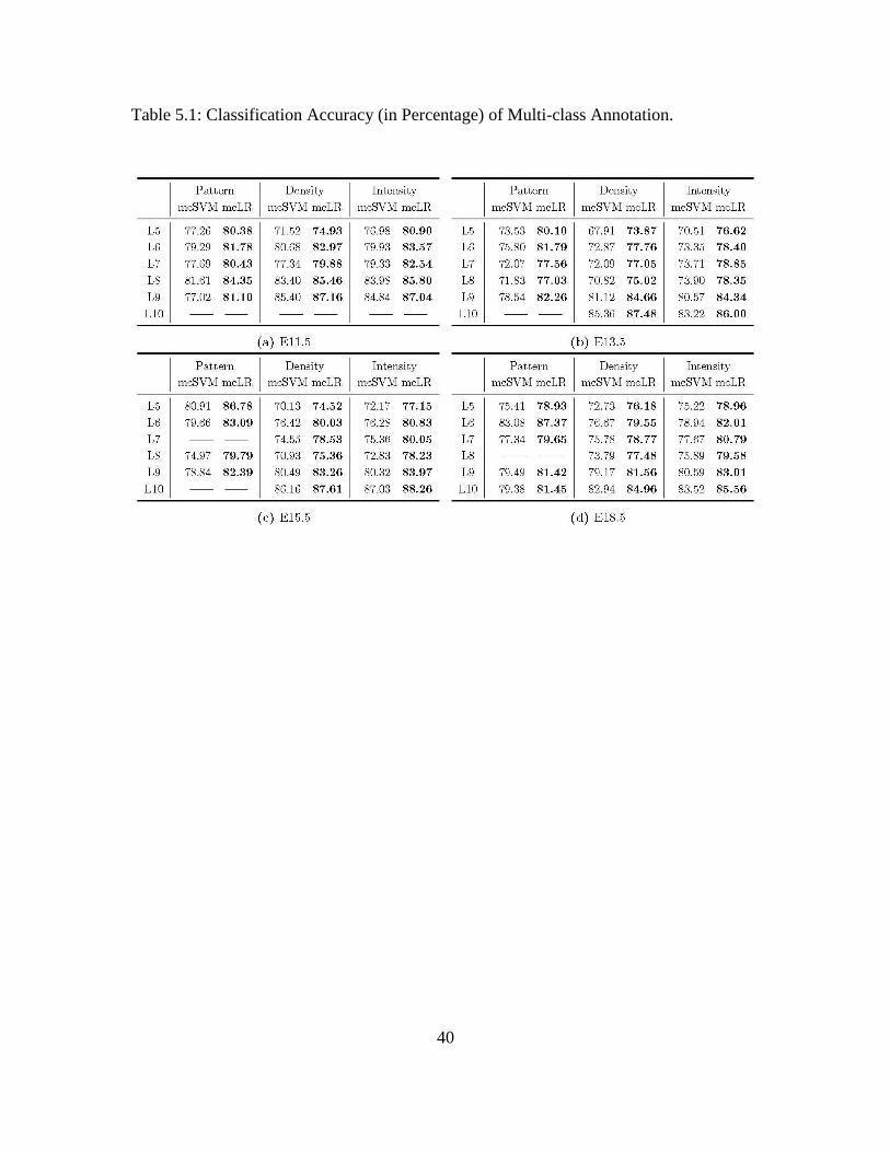
5.1: Classification Accuracy (in Percentage) of Multi-class Annotation. ........................ 40

5.2: Classification of Performance (AUC) of Structure-based Multi-label Annotation. .. 42

viii

LIST OF FIGURES

Figure Page

1.1: ISH Data in Allen Developing Mouse Brain Atlas. Four Levels (E.G. Undetected,

Full, Regional, and Gradient) of Expression in Three kinds (Patterns, Density, and

Intensity) of Metrics Are Used to Characterize the ISH Data. ........................................... 2

1.2: Percentages of the Four Categories of Gene Expression Status at Each Brain Level

from ISH Images in ADMBA. ............................................................................................ 5

1.3: Framework of Automatic Annotation Gene Expression Patterns Approach on Mouse

Brain Images. ...................................................................................................................... 7

2.1: Hierarchical Anatomic Ontology Structure of Mouse Brain from ISH, ADMBA [4].

(0-10 Levels Are Presented in the Figure, and the -1 Level and 11-13 Levels Have Been

Removed Due to the Irrelevance) ..................................................................................... 11

2.2: An Illustration of the Step-wise Annotation Propagation Throughout Anatomic

Ontology [4]. Two Kinds of Propagations: Propagation from Child to Parent and

Propagation from Parent to Child. .................................................................................... 13

2.3: An Illustration of the Framework of Undersampling-based Ensemble Method. The

Arrows Show the Data Processing Direction. Green Stands for Positive Class and Red

Stands for the Negative Class. M Stands for Models Generated by Different Training Sets.

P Stands for Prediction Results. ........................................................................................ 16

3.1: An Illustration of the Framework of Image-level Feature Extraction by Scale-

invariant Feature Transform Method to Generate Key-point Features. ............................ 20

3.2: An Illustration of the Framework of Feature Selection. Given Raw Images as Input,

Using SIFT, SCC, and Pooling Correspondingly to Output the Gene Level Descriptor. 23

ix

Figure Page

4.1: Framework of the Novel Structure-based Multi-label Classification Approach. The

First Prediction Task (Green Matrix) Stands for the First Phase (Generating Bottom Level

Prediction Probabilities), While the Second Prediction Stands for Classification Task

Based on This Augmented Training Set for the Remaining Levels. ................................ 29

5.1: Comparison of the Proposed Approach and Bag-of-word Method. “Mean" Group

Records the Average Performance of 11 Sub-models. “Vote" Group Records the

Performance of Using Majority Voting. ........................................................................... 35

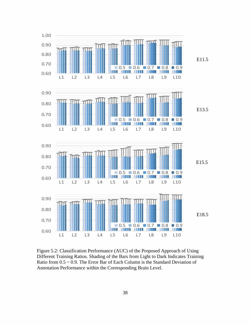
5.2: Classification Performance (AUC) of the Proposed Approach of Using Different

Training Ratios. Shading of the Bars from Light to Dark Indicates Training Ratio from

0.5 ~ 0.9. The Error Bar of Each Column is the Standard Deviation of Annotation

Performance within the Corresponding Brain Level. ....................................................... 38

1

Chapter 1

1. BACKGROUND AND INTRODUCTION

1.1 Background

Brain tumor is a fatal central nervous system disease and it is the second cause of

cancer in children [1]. Previous studies indicate that preventing and detecting brain

tumors at early stages are effective methods to reduce brain damage; these studies

also show the potential benefit of utilizing the genetic determinants [2]. Accurate

descriptions of the locations of where the relative genes are active and how these

genes express are critical for understanding the pathogenesis of brain tumor and for

early detection.

An accurate characterization of the gene expression and its role on brain

tumor requires extensive experimental resources on brain. A recent study [2] uses

mouse to reveal the genetic risk factor of brain cancer. However, such study was

performed on a limited set of genes. The Allen Developing Mouse Brain Atlas

(ADMBA) is an online public repository of extensive gene expression and

neuroanatomical data over different mouse brain developmental stages [3] [4]. The

knowledge is documented as high-resolution spatiotemporal in situ hybridization

(ISH) images for approximately 2,100 genes from embryonic through postnatal stages

of brain development. In addition, brain ontology has been designed to hierarchically

organize brain structure for the developing form of mouse brain, which facilitates

gene expression pattern annotation to specific brain areas. For a complete description

of the status of gene expression revealed by in situ hybridization, three kinds of

2

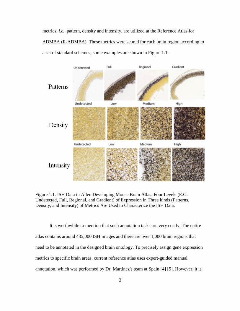
metrics, i.e., pattern, density and intensity, are utilized at the Reference Atlas for

ADMBA (R-ADMBA). These metrics were scored for each brain region according to

a set of standard schemes; some examples are shown in Figure 1.1.

Figure 1.1: ISH Data in Allen Developing Mouse Brain Atlas. Four Levels (E.G.

Undetected, Full, Regional, and Gradient) of Expression in Three kinds (Patterns,

Density, and Intensity) of Metrics Are Used to Characterize the ISH Data.

It is worthwhile to mention that such annotation tasks are very costly. The entire

atlas contains around 435,000 ISH images and there are over 1,000 brain regions that

need to be annotated in the designed brain ontology. To precisely assign gene expression

metrics to specific brain areas, current reference atlas uses expert-guided manual

annotation, which was performed by Dr. Martinez's team at Spain [4] [5]. However, it is

3

labor-intensive since it requires expertise in neuroscience and image analysis, and it does

not scale with the continuously expanding collection of images. Therefore, developing an

effective and efficient automated gene expression pattern annotation method is of

practical significance.

1.2 Challenges

Due to the specific biological application background and data attributes, the gene

expression annotation task is challenging in many aspects. In the following section, the

large data size challenge, multi-class challenge, imbalance data challenges and multi-

label challenge are discussed separately. The first two challenges are about the image

data which are provided by an online repository called Allen Developing Mouse Brain

Atlas (ADMBA). The other two are about challenges that are caused by different

requirements of specific applications, such as multi gene expression classification tasks

and classification based on the label hierarchy structure.

1.2.1 Large Data Size Challenge

As described in the Background section, the atlas we are dealing with is a large

scale dataset. All the gene information is documented in around 435,000 high-resolution

spatiotemporal ISH images. Those images are divided into four different embryonic

stages, called E11.5, E13.5, E15.5 and E18.5. Every stage contains about 2,100 genes,

and three metrics are applied to measure those genes. There are about 15 ~ 20 images on

each gene. Number of genes and images in each embryonic stage is shown in Table 1.1.

Moreover, the image sizes are not uniform, each image contains up to 12 million pixels.

The overall mouse brain is organized from level -1 to level 13, with -1 representing the

whole brain called “mouse”. We define over 1,000 brain areas based on this ontology.

4

Hence, dealing with such a big dataset and extract important features from it is a

challenge.

Table 1.1: The Sample Statistics of the Number of Genes and ISH Images in ADMBA

Stages # of Genes # of Images

E11.5 2071 35,659

E13.5 2064 35,396

E15.5 2070 35,864

E18.5 2022 35,506

1.2.2 Imbalanced Data Challenge

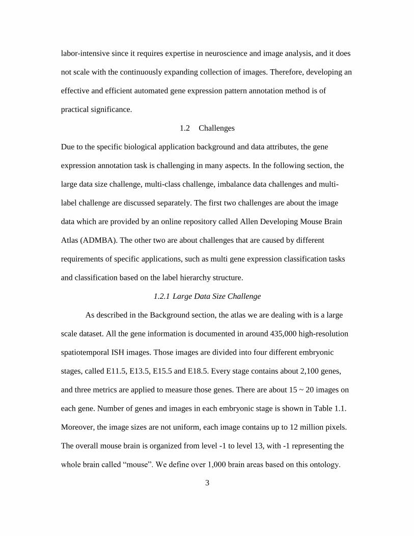
As an inherited characteristic, the data we are dealing with is very imbalanced. If we look

at the Figure 1.2, we can easily find that class distribution is very lack of balance. Take

pattern expression for an example, gene expression that marked as “Undetected” accounts

for the majority among the all four kinds of expressions in every brain level, while the

distribution of gene expression “Full” is much smaller. Since the imbalanced class

distribution is involved in each annotation task, traditional machine learning methods will

often be biased and fail to provide reliable models [6]. We need to do some preprocessing

steps first. I will discuss the techniques that we used in the following chapters.

5

Figure 1.2: Percentages of the Four Categories of Gene Expression Status at Each Brain

Level from ISH Images in ADMBA.

1.2.3 Multi-class Challenge

As mentioned in the first section, there are three different kinds of metric are applied to

describe the gene in each brain area. Based on each metric, four different types of

expression are defined. For a specific set of ISH images, current reference atlas uses up to

four categories (see Figure 1.1) to give an accurate description of the gene expression

status for a specific metric. Thus, the annotation problem we are facing is indeed a multi-

class classification problem.

1.2.4 Multi-label Challenge

Annotating gene expression pattern over the brain ontology is essentially a multi-label

classification problem. However, if we simply treat each label separately, we do not make

full use of the structural relationships among labels (as shown in Figure 2) in the learning

procedure, resulting in suboptimal prediction performance [7] [8]. How to take fully use

of the gene hierarchy during classification, is a big challenge here.

(a) Patten (b) Density (c) Intensity

6

1.3 Problem Setup

In this thesis, I focus on developing an effective and efficient automated gene expression

patterns annotation system. In this system, labels are automatically predicted with the

given metric in a specific brain area. There are essentially three objectives in this thesis:

Extract features based on Scale-Invariant Feature Transform (SIFT), and then

generate higher level features with Sparse Coding;

Develop accurate classifiers base on SVM and Logistic Regression that can

effectively and efficiently identify expression patterns for a given gene;

Improve the classifiers with the brain ontology structure of mouse; take advantage

of the label hierarchy.

1.4 Methods and Approaches

In this thesis, we propose an effective approach that can automatically annotate gene

expression patterns on mouse brain images. Since all the gene information is documented

in numerous high-resolution spatiotemporal in situ hybridization images, we firstly need

to extract low-level features from there raw images with scale-invariant feature transform

(SIFT) algorithm. SIFT has been commonly used in transforming image information to

local feature coordinates. These coordinates are invariant to translation, rotation, scale,

and other imaging parameters [9]. With the low-level features, we need to generate high-

level features. We use a novel sparse coding method, Stochastic Coordinate Coding, here

to combine features we get in former step. Both max-pooling and average-pooling are

applied on the gene level features generation to make sure we can get the best results.

Since there are three different metrics in each brain area and four categories for each

metric, the classification problem is in fact a multi-class problem. We first simply treat

7

this problem as a binary class issue, which means we classify the entire genes into

“detected” and “undetected”. Then we also solve the multi-class annotation problem via

multi-task learning. Robust machine learning algorithms such as Support Vector Machine

(SVM) and Logistic regression are applied in those classification problems. We also use

random undersampling and majority voting strategies to deal with the very imbalanced

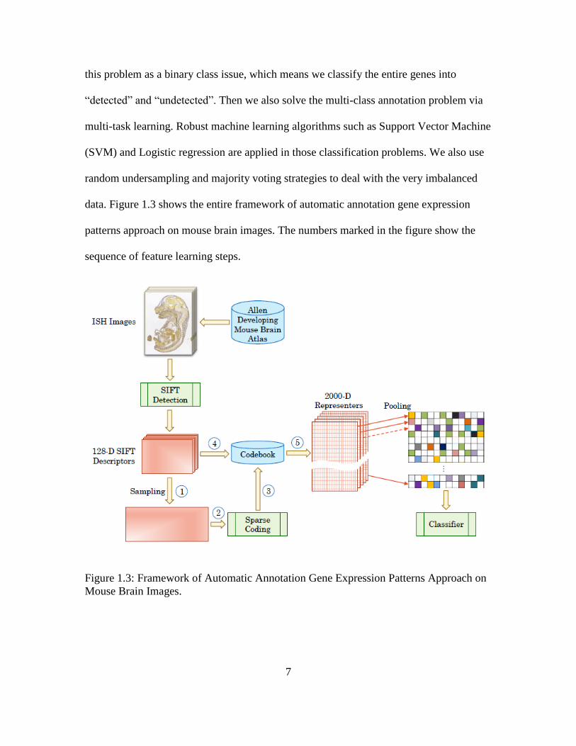
data. Figure 1.3 shows the entire framework of automatic annotation gene expression

patterns approach on mouse brain images. The numbers marked in the figure show the

sequence of feature learning steps.

Figure 1.3: Framework of Automatic Annotation Gene Expression Patterns Approach on

Mouse Brain Images.

8

In addition, we utilize the brain ontology to improve our method. Based on the

tree structure of anatomic ontology, the mouse brain is divided into 10 different levels.

Rather than learn the tasks individually, we find the performance is better with taking

advantage of the label hierarchy. Since the lower level nodes always achieve better

results, we utilize the bottom level nodes in building models. We first combine the

learned knowledge of bottom level nodes with the original tasks, and then lean new

models based on these new tasks.

The experimental results show that our approaches are robust and efficient. Our

method is proved to achieve relatively high accuracy even with a low training ratio and

the proposed novel label hierarchy based approach can significantly improve the

annotation accuracy at all brain ontology levels.

1.5 Thesis Organization

This thesis consists of five parts. Chapter 2 introduces the data and some preprocessing

steps we use. Chapter 3 focuses on the feature selection framework; we employ three

different steps to extract features from the raw images. Chapter 4 introduces some

classification methods; we primarily use SVM and logistic regression here. In chapter 5,

a novel approach based on mouse brain ontology is introduced in detail. Conclusion and

future work is listed in chapter 6.

9

Chapter 2

2. DATASETS AND PREPROCESSING

This chapter mainly describes the dataset that our gene expression annotation system

orients on and how these data images are preprocessed to be fed into the machine

learning framework properly. First, Allen Developing Mouse Brain Atlas (ADMBA) is

introduced in detail. All the data we used in this thesis can be downloaded from ADMBA.

Then the anatomic ontology tree of mouse brain is introduced, we take advantage of this

ontology and the corresponding propagation strategies in classification tasks. Finally,

based on the fact that our data is quite imbalance in distribution, the method that we used

to deal with imbalanced data is illustrated. After preprocessing, the calculated training

data will be used in model training in following chapters.

2.1 Data

The Allen Developing Mouse Brain Atlas is an extensive resource on gene expression

over the course of brain development from embryonic through postnatal stages, providing

both spatial and temporal information about gene expression [4]. The gene expression is

presented as in situ hybridization (ISH) data, which has been generated for approximately

2,100 genes at each of seven timepoints. The seven different timepoints consist of four

embryonic stages and three mature stages. We focus on the first four embryonic stages in

this study.

Users who are unfamiliar with mouse developmental anatomy can also benefit

from the experts-guided manually annotated ISH data. Three metrics are used to describe

gene expression: intensity, density, and pattern. Based on these given metrics, 1,075 brain

areas are annotated. It is important to note that not every brain area is manually annotated,

10

which amounts to over 1,500 areas, due to the unnecessary cost. The expert annotated in

each brain area provides an interpretation between the ISH images and the reference atlas

ontology.

2.2 Brain Ontology

As introduced in the former chapter, classifications with the learned features are not

effective enough. Base on the inherent characteristics, we find that taking advantage of

the label hierarchy will help improve classification accuracy. Thus, learning the mouse

brain ontology structure and the annotation propagation strategy is significant.

2.2.1 Ontology Structure

The Allen Developing Mouse Brain Atlas utilizes a single unified ontology for all ages,

based upon a topological ontogenetic viewpoint, such that brain structures in different

developmental timepoints can be roughly related by ontology despite the existence of

transient or migratory structures [4]. The brain is divided into several levels, which

marked as numbers from -1 to 13. The highest level (named -1) represents the entire

mouse, thus only one brain area in this level. Levels 11 to 13 represent individual brain

nuclei. In our study, we take advantage of the levels from level 1 to 10 since the first two

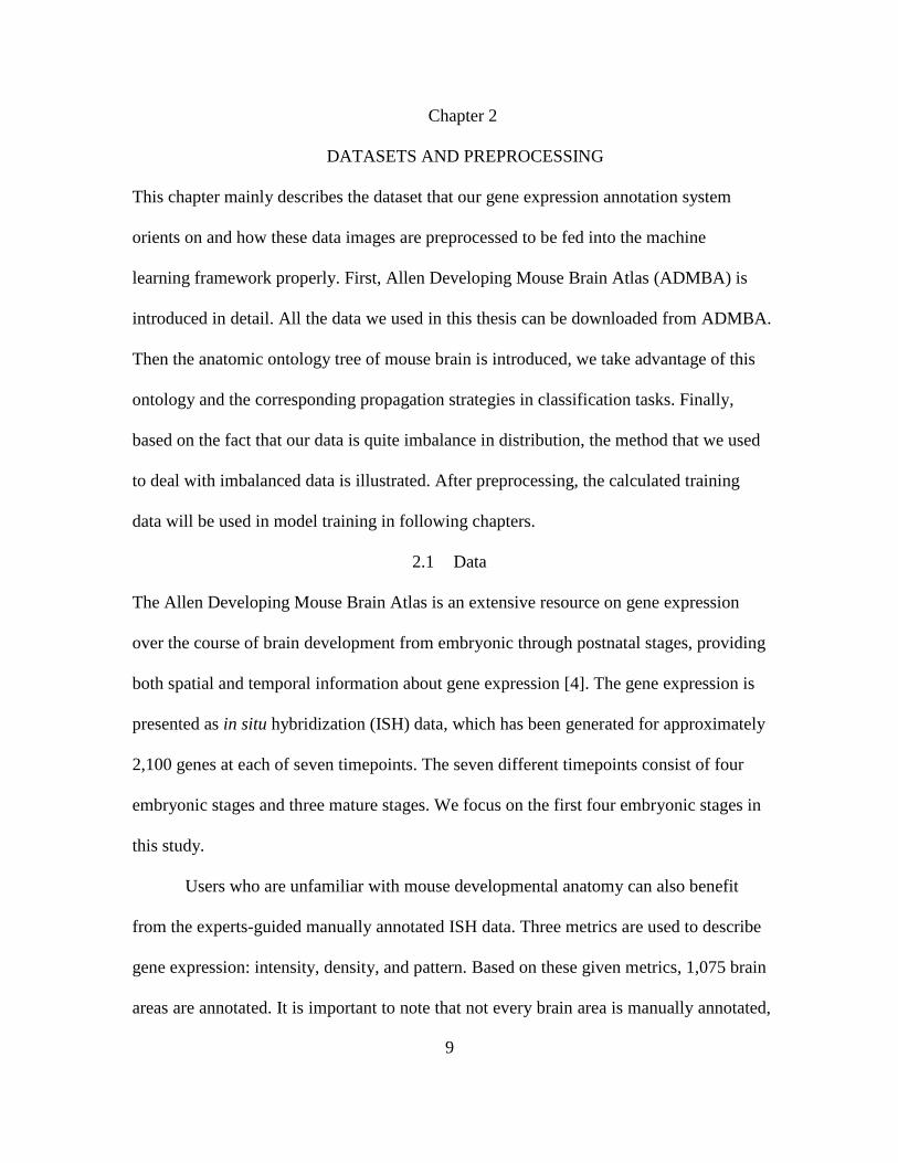
levels are not accurate enough and the last three levels are not annotated. Figure 2.1

roughly describes the ontology tree. Each node represents a brain area, and some brain

areas are omitted.

11

Figure 2.1: Hierarchical Anatomic Ontology Structure of Mouse Brain from ISH,

ADMBA [4]. (0-10 Levels Are Presented in the Figure, and the -1 Level and 11-13

Levels Have Been Removed Due to the Irrelevance)

2.2.2 Propagation Strategy

It is meaningful to mention that not every brain area is manually annotated due to the

goal of only covering every branch of the anatomic ontology tree. In practice, gene

expression annotations for both child structures and for parent structures are propagated

12

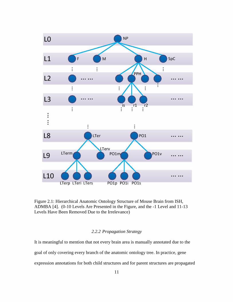
from a given annotated structure based upon a simple logic. [4] The logic is shown in

Figure 2.2. Manual annotated patterns are marked as green nodes in the graph. In B and C,

values are calculated with the annotation of children, while values are calculated for

children based on parents’ annotation information in D and E. Details of propagation of

annotation from child to parent and from parent to child are listed as follows:

Propagation of annotation to parent

In expression pattern of the parent calculation, we take use of the annotation of

child structures. In this case, all child structures must be annotated in order for the parent

to inherit annotation. For level and density, the parent structure received the highest

expression value of any of its children. The calculation logics are listed as below [white

paper]:

If all children = full, then the parent = full;

If all children = undetected, then the parent = undetected;

If the children possess different pattern values, then the parent = regional.

Propagation of annotation to child

The calculation logics are listed as below:

If a given structure was annotated, that expression data was assumed to apply

to all child structures;

If a parent has a pattern = full or undetected, then the children inherit all

annotation from that parent;

If the parent has a pattern = regional or gradient, then the children inherit

“cannot annotate”, because it is not possible to determine which child

structures should receive the expression calls.

13

Figure 2.2: An Illustration of the Step-wise Annotation Propagation Throughout

Anatomic Ontology [4]. Two Kinds of Propagations: Propagation from Child to Parent

and Propagation from Parent to Child.

2.3 Preprocessing

It is well known that most of existing learning systems are designed under the assumption

that the data have balanced class distributions. However, most biomedical data do not

satisfy this assumption in practice. In our study, regions in the brain ontology are divided

into 10 levels. Figure 1.2 shows the statistics of annotation distribution at each brain

ontology level. We can clearly observe that even for the binary classification case, the

data is severely imbalanced. Such an imbalanced data problem will lead to a bias toward

the majority in the following classification process. Thus, taking advantage of some data

processing method to deal with the imbalance problem is quite necessary in our study.

2.3.1 Imbalanced Data

A large number of standard learning algorithms assume that the distributions of two

classes are balanced or the misclassification costs are equal (or similar) to each other [4].

14

Imbalanced data means that the class distribution is not uniform among all the classes in

a dataset. Take binary class case as an example, we can find two classes, called majority

class and minority class, always differ greatly in size. Thus, using standard classification

methods without proper preprocessing steps always supposes a bias towards the majority

class.

Besides the inappropriate inductive bias problem, data imbalance will cause many

other challenges in machine learning. For instance,

Improper evaluation criteria

Absolute rarity and relative rarity

Noise

Thus, effective data preprocessing methods should be used to help the

performance of classification.

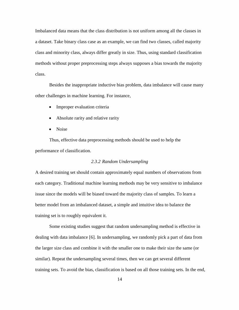
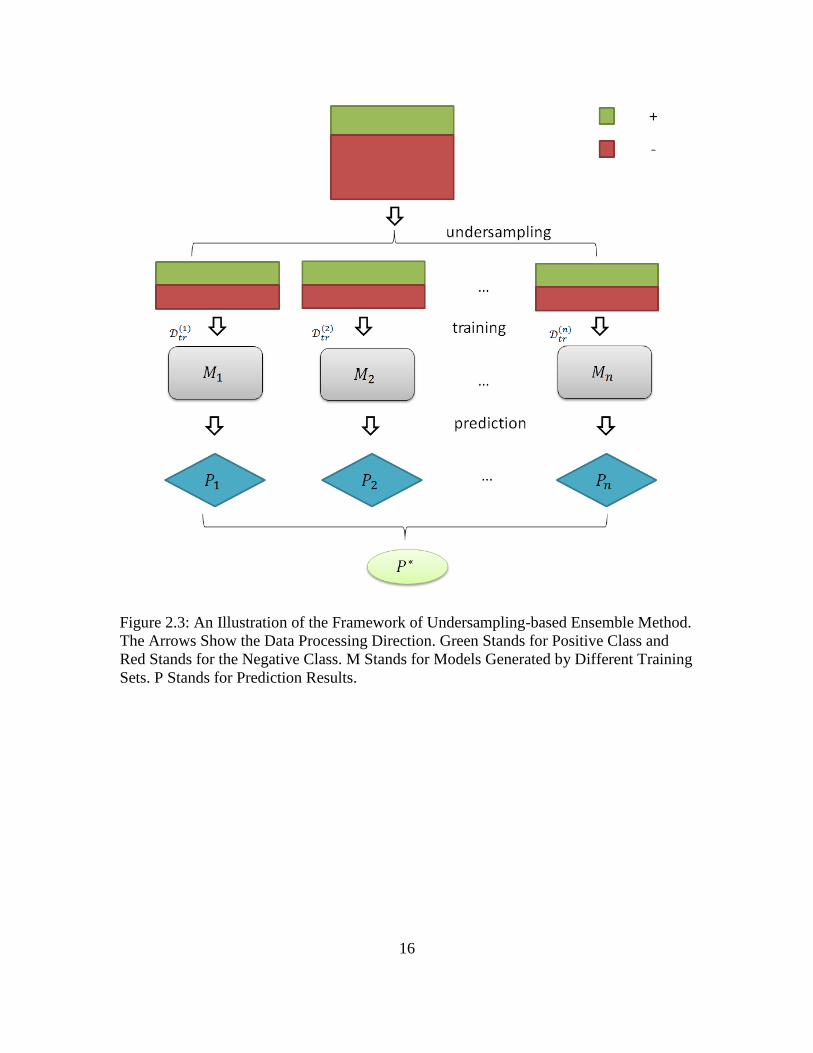
2.3.2 Random Undersampling

A desired training set should contain approximately equal numbers of observations from

each category. Traditional machine learning methods may be very sensitive to imbalance

issue since the models will be biased toward the majority class of samples. To learn a

better model from an imbalanced dataset, a simple and intuitive idea to balance the

training set is to roughly equivalent it.

Some existing studies suggest that random undersampling method is effective in

dealing with data imbalance [6]. In undersampling, we randomly pick a part of data from

the larger size class and combine it with the smaller one to make their size the same (or

similar). Repeat the undersampling several times, then we can get several different

training sets. To avoid the bias, classification is based on all those training sets. In the end,

15

we need to adopt majority voting to combine all results. Majority voting will be

introduced in the following chapter. This method is called undersampling-based

classifiers ensemble (UEM).

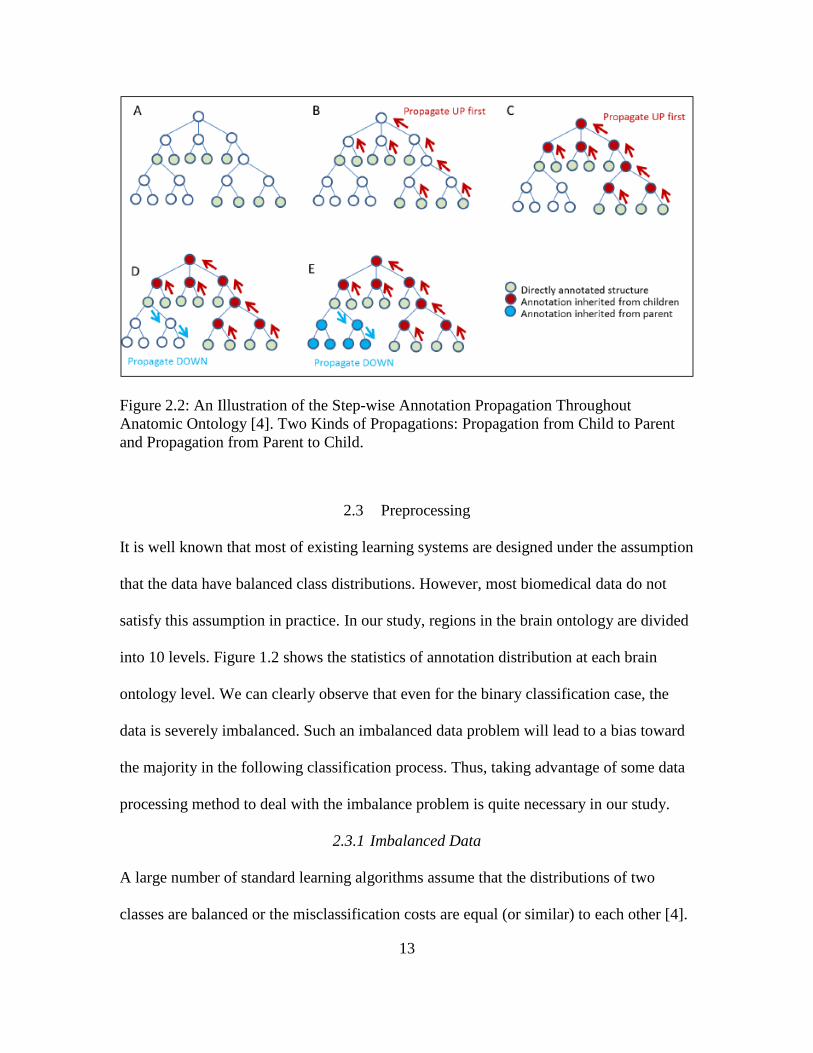
The framework of undersampling-based ensemble method is showed in Figure 2.3.

Green stands for minor class, while the red stands for majority. M stands for model and P

stands for prediction.

16

Figure 2.3: An Illustration of the Framework of Undersampling-based Ensemble Method.

The Arrows Show the Data Processing Direction. Green Stands for Positive Class and

Red Stands for the Negative Class. M Stands for Models Generated by Different Training

Sets. P Stands for Prediction Results.

17

2.4 Summary

In this chapter, I introduce the data we use in our approach. First, we talk about the online

gene expression repertory called Allen Developing Mouse Brain Atlas. Then we analyze

the inherent characteristics of the data, including expression patterns, pattern distributions

and the unified brain ontology. We find that the classification problem we are facing is

actually a multi-class and multi-label problem since the gene expression patterns are

defined in three metrics and four different categories are applied in each single metric. To

solve this multi-class and multi-label problem, we design an effective approach, which

will be introduced in the following chapters. Another challenge is the distribution of each

of the four categories is very imbalanced in every metric. Thus, we use random

undersampling as the data preprocessing step before classification.

18

Chapter 3

3. FEATURE SELECTION FRAMEWORK

As the effectiveness of annotation relies on the quality of feature representation, feature

selection is one of the most significant steps. In this chapter, I mainly focus on the

introduction of entire feature selection framework we used in our approach. The feature

selection consists of three different steps. First, we extract some image-level features

from raw images, we use a robust algorithm, called scale-invariant feature transform

(SIFT), those features are stored in 128-dimensional feature descriptors. Then we apply a

novel sparse coding method here to generate high-level features, experiments showed that

this method is very efficient compared with other traditional sparse coding methods. At

last, we need to combine those features to generate gene-level features. To generate those

representations, both max-pooling and average-pooling are used.

3.1 Learn from Feature Selection

The gene expression pattern annotation problem can be formulated as an image

annotation problem, which has been widely studied in computer vision and machine

learning. Specifically, a key to solve the problem is to learn effective feature

representations of images. The scale-invariant feature transform (SIFT) algorithm has

been commonly applied to transform image content into local feature coordinates that are

invariant to translation, rotation, scale, and other imaging parameters [9]. SIFT has been

shown to be a powerful tool to capture patch-level characteristics of images. Based on

those local image descriptors, the next step is to construct high-level feature

representations of the ISH images. A common approach is to use the bag-of-words (BoW)

model to represent high-level features, which has been used in a recent study [10].

19

However, BoW is not efficient to learn a large number of keywords or deal with large

scale data atlas. In this study, we employ sparse coding to construct high-level features,

which has been demonstrated to be effective in many fields including image recognition

[11]. Sparse coding aims to using sparse linear combinations of basis vectors to

reconstruct data vectors and learn a non-orthogonal and over-complete dictionary, which

has more exibility to represent the data [12] [13] [14]. The previous study [10] uses BoW

instead of sparse coding mainly due to the high computational cost of solving the sparse

coding problem especially for large-scale data in ADMBA. In this study, we adopt a

novel implementation of sparse coding, called Stochastic Coordinate Coding (SCC) [15],

which has been shown to be much more efficient than existing approaches.

3.2 Image-level Feature Extraction

Extracting and characterizing features from images is the key for image annotation. To

capture as much gene expression details as possible over the entire brain ontology,

ADMBA provides numerous spatiotemporal high-resolution ISH images. However, those

raw images are not well aligned since they were taken from different samples and at

different spatial slices. This makes it challenging to generate features from raw ISH

images. A commonly used approach in such case is to employ the well-known scale-

invariant feature transform method to construct local image descriptors. As shown in

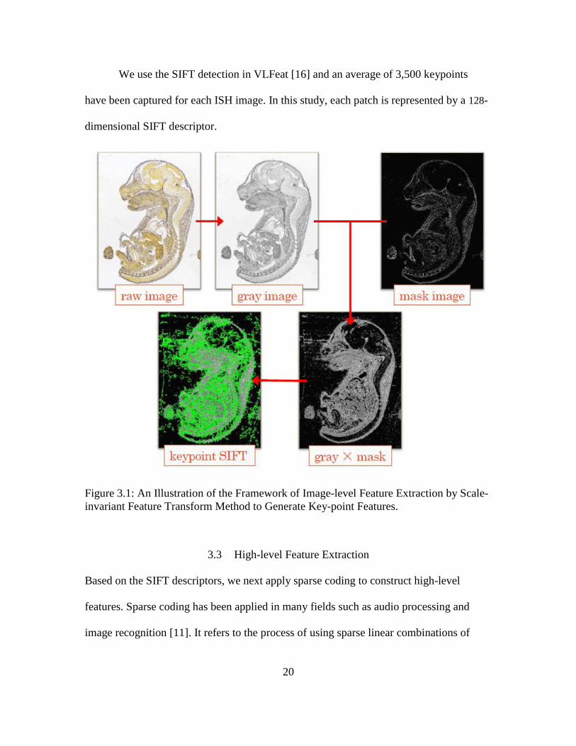
Figure 3.1, the framework of image-level feature extraction consists of several steps. The

SIFT method first detects multiple localized keypoints (patches) from a raw image, and

then transforms those image content into local feature coordinates that are invariant to

translation, rotation, scale, and other imaging parameters.

20

We use the SIFT detection in VLFeat [16] and an average of 3,500 keypoints

have been captured for each ISH image. In this study, each patch is represented by a 128-

dimensional SIFT descriptor.

Figure 3.1: An Illustration of the Framework of Image-level Feature Extraction by Scale-

invariant Feature Transform Method to Generate Key-point Features.

3.3 High-level Feature Extraction

Based on the SIFT descriptors, we next apply sparse coding to construct high-level

features. Sparse coding has been applied in many fields such as audio processing and

image recognition [11]. It refers to the process of using sparse linear combinations of

21

basis vectors to reconstruct data and learning a non-orthogonal, over-complete dictionary.

We can write the sparse coding problem as:

min

𝑫,𝒛𝟏,…,𝒛𝒏

∑(1

2‖𝑫𝒛𝑖 − 𝒂𝑖‖2

2 + 𝜆‖𝒛𝑖‖1 )

𝑛

𝑖=1

𝑠. 𝑡. ‖𝑫∙𝑗‖2

≤ 1, 1 ≤ 𝑗 ≤ 𝑝

(3.1)

where 𝑨 = [𝒂1, … , 𝒂𝑛] ∈ ℝ𝑚×𝑛 is the set of SIFT descriptors constructed from image

patches, each SIFT descriptor 𝒂𝑖 ∈ ℝ𝑚 is a m-dimension column vector with zero mean

and unit variance, 𝑫 ∈ ℝ𝑚×𝑝 is the dictionary, 𝜆 is the regularization parameter, and

𝒁 = [𝒛1, … , 𝒛𝑛] ∈ ℝ𝑝×𝑛 is the set of sparse feature representations of the original data. In

addition, to prevent D from taking arbitrarily large values, the constraint, 𝑫∙𝑗 , 1 ≤ 𝑗 ≤ 𝑝,

restricts each column of D to be in a unit ball.

Main steps of sparse coding method are listed as below:

1. Get a sample ai;

2. Learn the feature 𝑧i by fixing the dictionary 𝐷;

3. Update the dictionary 𝐷 by fixing the learned feature 𝑧I;

4. Normalize the dictionary 𝐷;

5. Go the Step 1 and iterate.

It has been known that solving the sparse coding problem is computationally

expensive, especially when dealing with large-scale data and learning a large size of

dictionary. The main computational cost comes from the updating of sparse codes and the

dictionary. In our study, we adopt a new approach, called Stochastic Coordinate Coding

(SCC), which has been shown to be much more efficient than existing methods [15]. The

key idea of SCC is to alternately update the sparse codes via a few steps of coordinate

22

descent and update the dictionary via second order stochastic gradient. In addition, by

focusing on the non-zero components of the sparse codes and the corresponding

dictionary columns during the updating procedure, the computational cost of sparse

coding is further reduced.

In our study, the dictionary is learned from SIFT descriptors of all ISH images.

The constraint, 𝒛𝑖 ≥ 0, 1 ≤ 𝑖 ≤ 𝑛, is further added to ensure the non-negativity of sparse

codes. To generate image-level features based on patch-level representations, we apply

the max-pooling operation. Max-pooling takes the strongest signal among multiple

patches to represent the image, which has been shown to be powerful in combining low-

level sparse features [17].

3.4 Gene-level Feature Extraction

Recall that a specific ISH image is obtained from particular brain spatial coordinates and

it may not be able to present the gene expression pattern over the entire brain ontology. In

order to describe expression pattern at all brain regions, we use a gene-level feature

pooling. Since it remains unclear what kind of pooling methods will perform better on

those high-level representations, both average-pooling and max-pooling are employed in

our study. In max-pooling approach, we take the most responsive value of the given

vector that stores all the features of a single gene, while we calculate average value of the

vector.

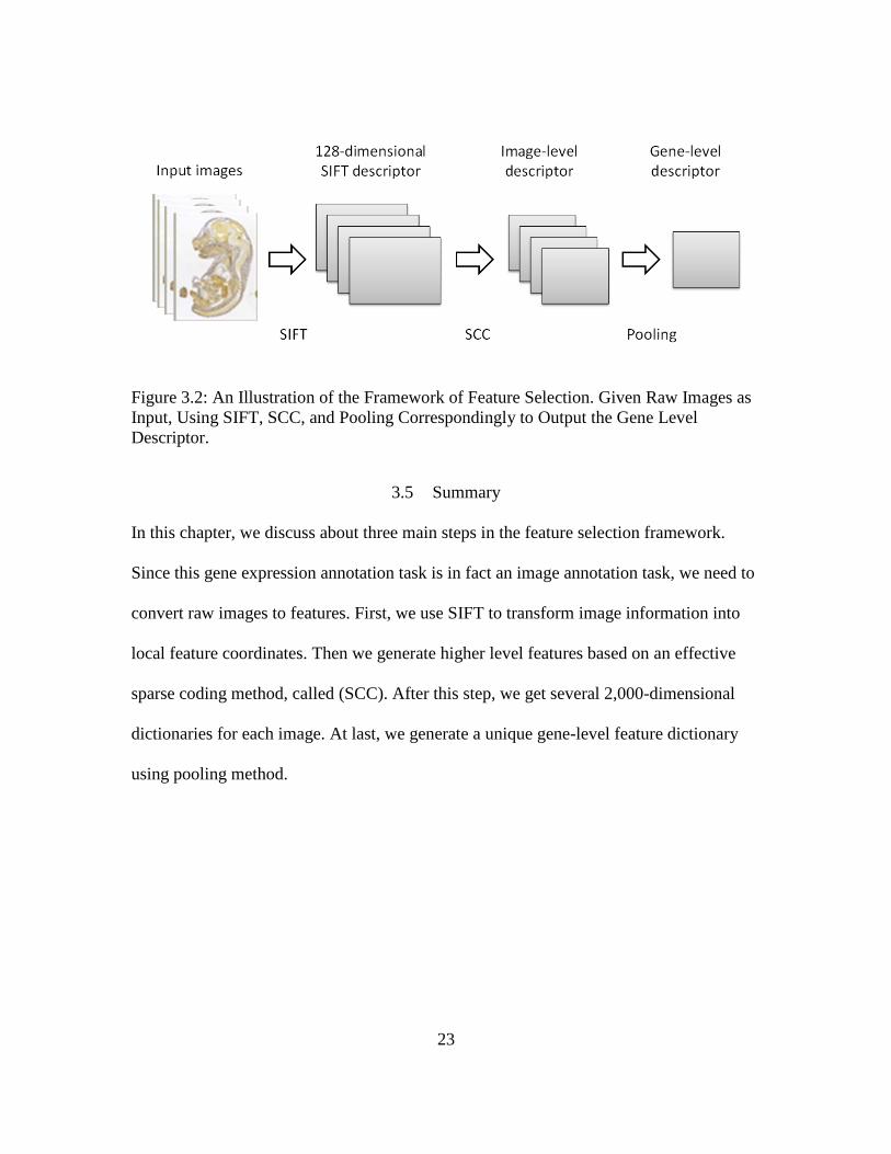
Figure 3.2 shows the framework of three-step feature selection. The input is raw

images, with SIFT, SCC and two kinds of pooling methods, a 2,000-dimensional feature

dictionary is generated.

23

Figure 3.2: An Illustration of the Framework of Feature Selection. Given Raw Images as

Input, Using SIFT, SCC, and Pooling Correspondingly to Output the Gene Level

Descriptor.

3.5 Summary

In this chapter, we discuss about three main steps in the feature selection framework.

Since this gene expression annotation task is in fact an image annotation task, we need to

convert raw images to features. First, we use SIFT to transform image information into

local feature coordinates. Then we generate higher level features based on an effective

sparse coding method, called (SCC). After this step, we get several 2,000-dimensional

dictionaries for each image. At last, we generate a unique gene-level feature dictionary

using pooling method.

24

Chapter 4

4. CLASSIFICATION METHODS

In this section, we introduce several regularized learning methods for gene expression

pattern classification. In our classification tasks, we use Support Vector Machine (SVM)

and Logistic Regression as classifiers. In addition, we present a structure-based multi-

label classification approach for annotation.

4.1 SVM

SVM [18], which is short for Support Vector Machine, is one of the most commonly

adopted methods for classification, and regression analysis. The design rationale of SVM

is to project all training data points into a hyperplane or hyperplanes, find a wide clear

gap to separate the data points and the space, and classify the new data according to their

projections on the hyperplane.

Formally, the SVM would construct a hyperplane or a set of hyperplanes

(depending on the dimension requirements of the data) and project the training data into

the space. The projection may be linear or nonlinear. With the help of the SVM training

algorithm, these training data points are separated by a gap on the hyperplane(s), which

comes across no data point. The gap is required to be as wide as possible to efficiently

classify the data, as with the wider the gap comes with a lower classification error. To

decide the category of each data, SVM simply project the data onto the hyperplane(s) and

observe the group of data points it belongs to.

Since SVM has already been widely studied and adopted by a large body of

researches, in this thesis we use SVM as a black box test. We apply SVM on the data

25

classification, use this result as a benchmark, and compare it with our own proposed

methods.

4.2 Binary-class Sparse Logistic Regression

We first consider the simple case, binary classification. Specifically, for a certain metric

of gene expression, we convert the original annotation task into a binary classification

problem by treating the category “undetected" as one class and all remaining categories

as the other class. We employ the regularized supervised learning methods, which have

been widely used in machine learning and bioinformatics. Let 𝐗 = {𝑥𝑖}𝑖=1𝑛 ∈ ℝ𝑛×𝑝

denote a dataset with n observations and p dimension, and 𝒚 = {𝑦𝑖}𝑖=1𝑛 ∈ ℝ𝑛×1, 𝑦𝑖 ∈

{−1, 1} be the corresponding labels. Then, we can write the sparse logistic regression

problem as follows:

min𝒘

ℒ(𝐗𝐰, 𝐲) + 𝜆‖𝐰‖1 (4.1)

where ℒ(∙) denotes the logistic loss, 𝐰 ∈ ℝ𝑝×1 is the model weight vector and 𝜆 is the l1-

norm regularization parameter. The solution of the above system will yield sparsity in w,

and the significant columns of X are determined by the corresponding non-zero entries in

w. In our study, 𝒙𝑖 is a gene-level representation of ISH images and 𝒚𝑖 encodes the

annotation of gene expression status for a specific brain region.

4.3 Multi-task Sparse Logistic Regression

We also propose to directly solve the multi-class annotation problem via multi-task

learning. Suppose there are k classes (k = 3 or 4 in our study). We can represent the

category of a sample by a k-tuple, where 𝑦𝑘𝑖 = 1 if sample i belongs to class k and

𝑦𝑘𝑖 = −1 otherwise. Then we can rewrite the response Y as 𝐘 = {𝑦𝑖}𝑖=1𝑛 ∈ ℝ𝑛×𝑘. We

26

employ the following multi-task sparse logistic regression formulation for the multi-class

case:

min𝐖

ℒ(𝐗𝐖, 𝐘) + 𝜆‖𝐖‖2,1 (4.2)

where 𝐖 ∈ ℝ𝑝×𝑘, and the i-th column of W is the model weight for the i-th task. The l2,1-

norm penalty on W results in grouped sparsity, which restricts all tasks to share a

common set of features. In this thesis, we employ such multi-task model to solve the

multi-class annotation problem. We utilize the SLEP [19] package to solve both of

problem 4.1 and problem 4.1.

4.4 Majority Voting

Besides undersampling, model ensemble is also beneficial for learning from imbalanced

data [20]. Ensemble methods refer to the process of combining multiple models to

improve predictive performance. In ensemble method, a significant step is using majority

voting to combine all the prediction result. Majority rule is to select alternatives that are

the majority in complete works. We can see how majority voting work in undersampling-

based ensemble method in Figure 2.3. We can get several prediction results from all the

models generated from last step. With these results, we get the final value of

corresponding gene by voting for the majority.

The idea of classifier ensemble is to build a prediction model by combining a set

of individual decisions from multiple classifiers [21]. In this study, we employ

undersampling multiple times; combine a set of learning models, one for each

undersampled data, and finally use majority voting to infer the predictions.

27

4.5 Structure-based Multi-label Annotation over Brain Ontology

Annotating gene expression patterns over the brain ontology is indeed a multi-label

classification problem. In the reference atlas, the expression patterns of a single gene are

recorded based on a hierarchically organized ontology of anatomical structures. In

practice, it is possible to propagate annotation to parent or child structures under a set of

systematic rules [4]. Rather than simply treating each individual annotation task

separately, if we build all prediction models together by utilizing the structure

information among labels, the predictive performance can potentially be significantly

improved [7] [17].

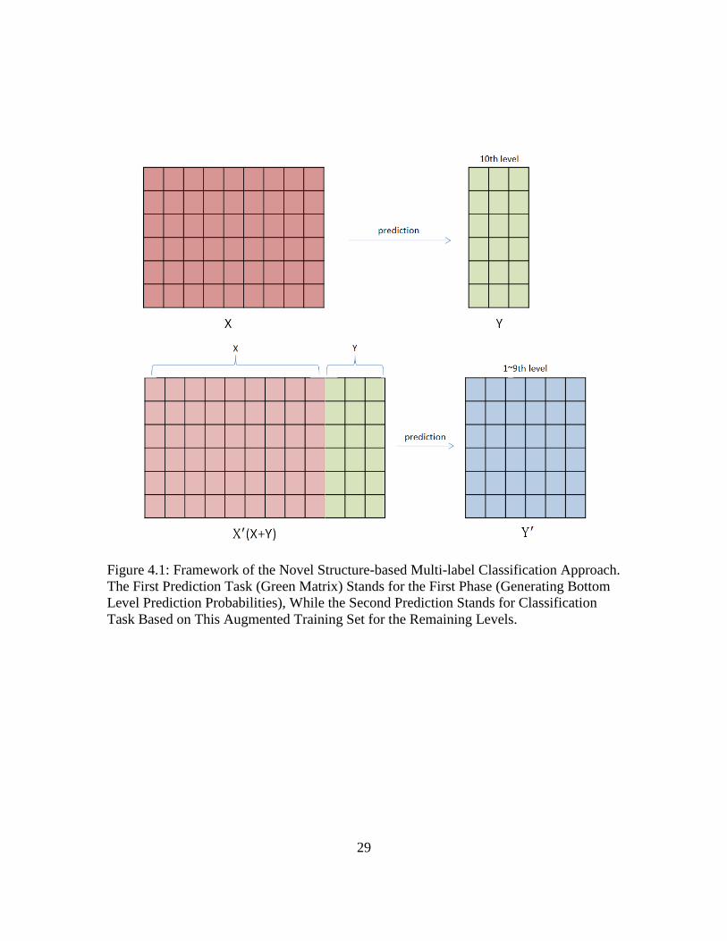
In this study, we propose a novel structure-based multi-label classification

approach. Suppose we are given n training data points {(𝐱𝑖, 𝐲𝑖)}𝑖=1

𝑛, where 𝐱𝑖 ∈ ℝ𝑝 is a

data point of p features, and 𝐲𝑖 ∈ ℝ𝑘 is the corresponding label vector of k tasks. Let

𝑗 ∈ {1, … , 𝑘} denote the j-th learning task. We then divide the learning procedure into two

phases. Assuming there are t tasks (t < k) at the bottom level of the hierarchy, in the first

phase, each of those tasks is learned individually by:

�̃�𝑗 = ℱ𝑗(�̃�), 1 ≤ 𝑗 ≤ 𝑡 < 𝑘 (4.3)

where ℱ𝑗(∙) denotes a learnt model by the j-th task, �̃� ∈ ℝ𝑝 is an arbitrary data point, and

�̃� ∈ ℝ is the prediction of �̃� for the j-th task. The green matrix in Figure 4.1 stands for the

prediction result of bottom level (10-th level in our dataset) in brain ontology, the model

is learned from the original training set (shown as red matrix in Figure 4.1). The learned

knowledge in formula above is used to learn the remaining tasks (𝑖. 𝑒. , 𝑡 + 1 ≤ 𝑗 ≤ 𝑘) in

the second phase. Specifically, we augment the feature set by adding the prediction

probabilities learnt in the previous phase, i.e., we denote �̃�′ = [�̃�, (�̃�1, … , �̃�𝑡)] (shown as

28

matrix X′ in Figure 4.1). Annotation tasks in the second phase will be performed based on

this augmented feature set �̃�′.

The tasks in the first phase can be considered as the auxiliary tasks in the second

phase [22]. We apply the two-stage approach in our case since the tasks are not

symmetric due to the hierarchical label structure. With the prediction probabilities from

the previous learning phase, we make use of label dependency along with the original

image representations. Intuitively, if a new learning task is related to some of the tasks

learnt in the first phase, then such approach is expected to achieve better classification

accuracy. In our study, since the tasks associated with the bottom of the label hierarchy

are related to the remaining tasks in the hierarchy, the prediction performance is expected

to be improved by the two-stage learning approach. This is confirmed in our experiments

presented in the following chapter. Figure 4.1 shows the framework of this two phases

approach.

29

Figure 4.1: Framework of the Novel Structure-based Multi-label Classification Approach.

The First Prediction Task (Green Matrix) Stands for the First Phase (Generating Bottom

Level Prediction Probabilities), While the Second Prediction Stands for Classification

Task Based on This Augmented Training Set for the Remaining Levels.

30

4.6 Summary

In this chapter, we talk about some popular methods to deal with classification and we

utilize those methods in our experiments, which will be further discussed in the following

chapter. Support Vector Machine (SVM) and Logistic Regression are two well-known

machine-learning algorithms. We apply both binary classification and multi-class

classification with Logistic Regression. Moreover, we also propose a novel gene

hierarchy based method in classification tasks. Since the lower level annotation tasks

always achieve higher performance, taking advantage of them will improve the overall

performance. In our method, prediction probabilities of bottom level are used to augment

the feature set.

31

Chapter 5

5. EXPERIMENTS AND RESULTS

In this chapter, I introduce how we design the experiments, the results and the

achievement of our methods. We design a series of experiments to evaluate the proposed

approach for gene expression pattern annotation on the Allen Developing Mouse Brain

Atlas. Specifically, we evaluate our approach in the following four aspects:

Comparison of sparse coding and bag-of-words

Comparison of different training ratios

Comparison of different multi-class annotation methods

Comparison of annotation with and without brain ontology

The undersampling-based classifiers ensemble framework (shown in Figure 2.3)

is used to deal with the imbalanced dataset. The results show that our approach is

effective and efficient.

5.1 Data Description and Experimental Setup

The gene expression ISH images are obtained from the Allen Developing Mouse Brain

Atlas. Specifically, to ensure the consistency of brain ontology over different mouse

developmental stages, we focus our experiments on the four embryonic stages, namely,

E11.5, E13.5, E15.5 and E18.5. The ADMBA provides approximately 2,100 genes within

each stage and an average of 15 ~ 20 images are used for each gene to capture the

expression information over the entire 3D brain. The total number of ISH images in these

four stages is 142,425. We use the SIFT method to detect local gene expression and apply

sparse coding to learn sparse feature representations for image patches. Considering the

resolution of the ISH images and the number of areas of the mouse brain ontology, a

32

dictionary size of 2,000 is chosen, i.e., 𝑫 ∈ ℝ128×2000. To generate gene-level

representations, both max-pooling and average-pooling are used.

To evaluate the effectiveness of the proposed methods, we compare our approach

with the well-known bag-of-words (BoW) method. Specifically, the BoW was performed

in two different settings:

The first approach, called non-spatial BoW, which concatenates three BoW

representations of SIFT features, where each BoW is learned from the ISH images at a

specific scale. The second approach, called spatial BoW, divides the brain sagitally into

seven intervals according to the spatial coordinate of each image, and then 21 regional

BoW representations are built (7 intervals × 3 scales) [10]. At each scale, a fixed number

of 500 clusters (keywords) are constructed from SIFT features and an extra dimension is

used to count the number of zero descriptors.

R-ADMBA uses three different metrics including pattern, density and intensity, to

evaluate the gene expression pattern on each brain ontology area. As discussed in the

previous section, we consider the annotation tasks as either binary-class or multi-class

classification problem. For the simple binary-class case, the category “undetected" is

treated as the negative class, which refers to the scenario that no gene expression pattern

is detected at the specific brain area, and all remaining categories are treated as the

positive class, which means some kind of expression pattern has been detected. It is

worthwhile to note that, at such a binary-class situation, if the annotation metric “pattern”

is marked as “undetected”, then metrics “density” and “intensity” must be “undetected”,

and vice versa. That is, it is possible to use a single metric to evaluate the gene expression

statues in this case.

33

In addition, in order to balance the class distributions of training sets, random

undersampling is performed for 11 times. To give a baseline performance of the

traditional method, the experiment results of using Support Vector Machine (SVM)

classifier [23] is also reported. To better describe the classification performance under the

circumstances of data imbalance, we use the area under the curve (AUC) of a receiver

operating characteristic (ROC) curve as the performance measure for binary-class

classification. The accuracy is used as the performance measure for the multi-class case.

5.2 AUC and Accuracy

In three of experiments, we used area under the curve (AUC) instead of accuracy as a

metric of the binary classification results.

Accuracy, which computes the proportion of true positives and negatives

(sometimes including false positives and negatives as well), is the most commonly used

metric for the classification result. A commonly adopted definition of accuracy is given

as follows:

true positives + true negatives

true positives + false positives + false negatives + true negatives

However, when it comes to probabilistic model where over fitting may happen or

the false positive and true positive rates are computed when above a random threshold,

accuracy reaches its limitation since the threshold may not be "good and accurate".

Thus, in this thesis, we use AUC instead of the accuracy since AUC may present

a more comprehensive prediction of the classifier efficiency. AUC is applied to the

binary classifiers and balances the trade-off between true positives and negatives since it

is not a function of probabilistic thresholds. The curves of the true positives rate against

34

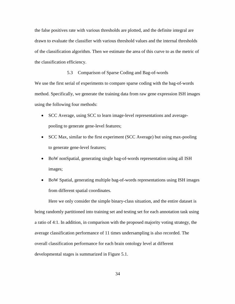
the false positives rate with various thresholds are plotted, and the definite integral are

drawn to evaluate the classifier with various threshold values and the internal thresholds

of the classification algorithm. Then we estimate the area of this curve to as the metric of

the classification efficiency.

5.3 Comparison of Sparse Coding and Bag-of-words

We use the first serial of experiments to compare sparse coding with the bag-of-words

method. Specifically, we generate the training data from raw gene expression ISH images

using the following four methods:

SCC Average, using SCC to learn image-level representations and average-

pooling to generate gene-level features;

SCC Max, similar to the first experiment (SCC Average) but using max-pooling

to generate gene-level features;

BoW nonSpatial, generating single bag-of-words representation using all ISH

images;

BoW Spatial, generating multiple bag-of-words representations using ISH images

from different spatial coordinates.

Here we only consider the simple binary-class situation, and the entire dataset is

being randomly partitioned into training set and testing set for each annotation task using

a ratio of 4:1. In addition, in comparison with the proposed majority voting strategy, the

average classification performance of 11 times undersampling is also recorded. The

overall classification performance for each brain ontology level at different

developmental stages is summarized in Figure 5.1.

35

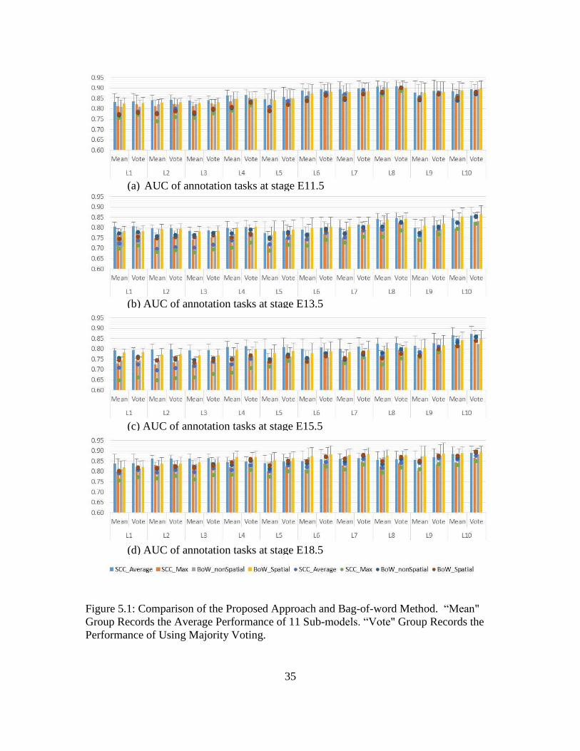
Figure 5.1: Comparison of the Proposed Approach and Bag-of-word Method. “Mean"

Group Records the Average Performance of 11 Sub-models. “Vote" Group Records the

Performance of Using Majority Voting.

(a) AUC of annotation tasks at stage E11.5

(b) AUC of annotation tasks at stage E13.5

(c) AUC of annotation tasks at stage E15.5

(d) AUC of annotation tasks at stage E18.5

36

In Figure 5.1, each column bar represents the performance of using sparse logistic

regression classifier for a specific set of gene-level image representations. Each dot

represents the performance of using SVM classifier for a specific set of gene-level image

representations. The error bar of each column is the standard deviation of annotation

performance within the corresponding brain level.

We can observe from Figure 5.1 that the proposed approach achieves the highest

overall AUC of 0.9095, 0.8573, 0.8717 and 0.8903 at mouse brain developmental stages

E11.5, E13.5, E15.5 and E18.5 respectively. For the comparison of different types of

image representations, SCC Average provides the best overall performance among all

four stages. Although in some annotation tasks, BoW Spatial provides competitive

performance to SCC Average, it is worthwhile to note that, the spatial BoW ensembles 21

single dictionaries and contains more than 10,000 features. Thus, spatial BoW is far more

complex than SCC and involves higher computational costs. We can also observe that the

use of undersampling and majority voting strategies improves the individual model by 1%

~ 3% in terms of AUC. Moreover, in comparison with SVM classifier, the sparse logistic

regression classifier achieves better predictive performance. Those experimental results

verify the superiority of our proposed methods.

5.4 Comparison of Different Training Ratios

In this experiment, we compare the classification performance of using different training

ratios. More specifically, we would like to verify the robustness of the presented

approach when using a relatively small number of samples for training. According to the

first serial of experiments, we use the SCC Average to construct features in this

experiment. For each annotation task, we fix 10% of the samples as testing set and vary

37

the ratio of training set in {50%, 60%, 70%, 80%, and 90%}. The experimental results

are summarized in Figure 5.2.

We can observe from Figure 5.2 that, at all four mouse brain developmental

stages and all brain levels, no significant difference is observed between different training

ratios. We can conclude from this experiment that our proposed approach is robust even

with a low training ratio, thus accurate models for gene expression annotation can be

learned based on a relative small number of manually annotated images.

38

Figure 5.2: Classification Performance (AUC) of the Proposed Approach of Using

Different Training Ratios. Shading of the Bars from Light to Dark Indicates Training

Ratio from 0.5 ~ 0.9. The Error Bar of Each Column is the Standard Deviation of

Annotation Performance within the Corresponding Brain Level.

0.60

0.70

0.80

0.90

1.00

L1 L2 L3 L4 L5 L6 L7 L8 L9 L10

0.5 0.6 0.7 0.8 0.9

0.60

0.70

0.80

0.90

L1 L2 L3 L4 L5 L6 L7 L8 L9 L10

0.5 0.6 0.7 0.8 0.9

0.60

0.70

0.80

0.90

L1 L2 L3 L4 L5 L6 L7 L8 L9 L10

0.5 0.6 0.7 0.8 0.9

0.60

0.70

0.80

0.90

L1 L2 L3 L4 L5 L6 L7 L8 L9 L10

0.5 0.6 0.7 0.8 0.9

E11.5

E13.5

E15.5

E18.5

39

5.5 Comparison of Different Multi-class Annotation Methods

In this experiment, we evaluate our multi-task sparse logistic regression (mcLR)

approach in the multi-class annotation situation. Dataset SCC Average is employed and

we use the multi-class SVM (mcSVM) as the baseline for performance comparison. In

this experiment, 80% of the samples from each class are randomly chosen as the training

set, and the remain 20% of the samples are used as the testing set. We only include

annotation classes if there are more than 100 samples available for a specific class. The

accuracy is used as the performance measure and the results are reported in Table 5.1.

We can observe from Table 5.1, our proposed approach using sparse logistic

regression with grouped sparsity constraint provides favorable predictive accuracy for

this multi-class annotation task. Specifically, the classification accuracy of mcLR is

significantly higher than mcSVM at all brain stages and levels. All detailed gene

expression status measured by pattern, density and intensity can be well distinguished by

our classifiers. These results imply that those multiple classes are inherently related and it

is beneficial to learn four (or three) classification models simultaneously by restricting all

models to share a common set of features. We plan to explore other multi-task learning

models in our future work [24].

40

Table 5.1: Classification Accuracy (in Percentage) of Multi-class Annotation.

41

5.6 Comparison of Annotation With and Without Brain Ontology

Recall that the expert-guided manual annotations are based on a hierarchically organized

ontology of anatomical structures. Rather than learning each task individually, it may be

beneficial to utilize the hierarchy among the labels for a joint annotation. As we can

observe from previous experiments, models learned in a lower level typically have better

predictive performance. Thus, it is natural to make use of the lower-level models and

label structures to improve the prediction performance of high-level tasks.

In this study, we compare our proposed structure-based multi-label learning

(SMLL) method with the simple individual annotation, which builds models for different

tasks independently. Again, we employ the SCC Average method to construct the data.

At each brain developmental stage, around 140 genes are randomly preselected as the

testing set for the annotation tasks over the entire brain ontology and the remaining genes

are included in the training set. For SMLL method, 432 tasks (regions) at level 10 (L10)

are learned individually in the first phase. The prediction probabilities of L10 tasks will

be used as the additional features in the data. In this experiment, we consider the binary-

class situation and results are summarized in Table 5.2.

We can observe from Table 5.2 that the overall annotation performance achieved

by SMLL is higher than the individual model. Improvements in terms of AUC can be

observed at most of the brain ontology levels among all developmental stages. This

verifies the effectiveness of the proposed structured-based multi-label learning approach.

42

Table 5.2: Classification of Performance (AUC) of Structure-based Multi-label

Annotation.

43

5.7 Summary

In this chapter, I introduce several experiments we design to evaluate our approach and

analyze the experimental results. We use area under the curve (AUC) and accuracy as the

metrics in our experiments. The results show that our approach is effective and robust on

both binary-class case and multi-class case. Compared with the well-known bag-of-words

(BoW) method, our sparse coding based approach is proved more effective and accurate.

Moreover, the proposed structure-based multi-label annotation method improves the

classification results significantly.

44

Chapter 6

6. CONCLUSION AND FUTURE WORK

In this thesis, we propose an efficient approach to perform automated gene expression

pattern annotation on mouse brain images. During the design of the automatic gene

expression annotation approach, different algorithms are used to annotate the gene

expression patterns on mouse brain images. With the SIFT algorithm and augmented

sparse coding method, our approach succeeds to annotate the high dimensional data with

a higher accuracy and a better efficiency. Using undersampling-based ensemble method,

the approach accomplishes the annotation tasks by combining the results from different

models. We use AUC and accuracy as the evaluation metric, results show that the

approach can achieve a satisfactory performance even with a low training ratio. With the

proposed ontology structure based multi-label approach, we find that using low level

annotations in further classification tasks improves the results significantly.

Our approach can be summarized as several steps. First, the key information in

spatiotemporal in situ hybridization images is captured by the SIFT method from local

image patches. Image-level features are then constructed via sparse coding. To generate

gene-level representations, different pooling methods are adopted. Regularized learning

methods are employed to build classification models for annotating gene expression

pattern at different brain regions. To utilize hierarchal information among the brain

ontology, a novel structure-based multi-label classification approach is proposed.

Extensive experiments are conducted on the atlas and the results demonstrate the

effectiveness of the proposed approach.

45

The future work can be divided into two parts. One of our future directions is to

explore deep learning models to learn feature representations from ISH images. Deep

learning is a branch of machine learning and it focuses on using multiple processing

layers with complex structures. The other one is to explore other multi-task learning

models to make a more effective usage of the hierarchal labels in the annotation. Multi-

task learning may lead to a better model because it combines several related problems

and thus may product results that satisfy the requirement from these related problems.

46

7. REFERENCES

[1] W. A. Bleyer, "Epidemiologic impact of children with brain tumors," Child's

Nervous System, vol. 15, no. 11-12, pp. 758--763, 1999.

[2] K. M. Reilly, "Brain Tumor Susceptibility: the Role of Genetic Factors and Uses

of Mouse Models to Unravel Risk," Brain Pathology, pp. 121--131, 2009.

[3] A. I. f. B. Science, "Allen Developing Mouse Brain Atlas," 2013. [Online].

Available: http://developingmouse.brain-map.org.

[4] A. D. M. B. ATLAS, "Allen Developing Mouse Brain Atlas technical white

paper," 2013.

[5] C. L. Thompson, L. Ng, V. Menon and S. Martinez, "A High-Resolution

Spatiotemporal Atlas of Gene Expression of the Developing Mouse Brain,"

Neuron, pp. 309--323, 2014.

[6] H. He and E. Garcia, "Learning from imbalanced data," Knowledge and Data

Engineering, IEEE Transactions on, vol. 21, pp. 1263--1284, 2009.

[7] C. N. Silla Jr and A. A. Freitas, "A survey of hierarchical classification across

different application domains," Data Mining and Knowledge Discovery, vol. 22,

pp. 31--72, 2011.

[8] G. Tsoumakas, I. Katakis and I. Vlahavas, "Mining multi-label data," in Data

mining and knowledge discovery handbook, Springer, 2010, pp. 667--685.

[9] D. Lowe, "Object recognition from local scale-invariant features," Computer

Vision, 1999. The Proceedings of the Seventh IEEE International Conference on,

vol. 2, pp. 1150--1157, 1990.

[10] T. Zeng and S. Ji, "Automated Annotation of Gene Expression Patterns in the

Developing Mouse," 2014.

[11] A. Szlam, K. Gregor and Y. LeCun, "Fast Approximations to Structured Sparse

Coding and Applications to Object Classification," in Computer Vision – ECCV

2012, Springer Berlin Heidelberg, 2012, pp. 200-213.

[12] B. A. Olshausen and D. J.Field, "Emergence of simple-cell receptive field

properties by learning a sparse code for natural images," Nature, vol. 381, pp.

607--609, 1996.

47

[13] S. S. Chen, D. L. Donoho and M. A. Saunders, "Atomic decomposition by basis

pursuit," SIAM journal on scientific computing, vol. 20, pp. 33--61, 1998.

[14] D. L. Donoho and M. Elad, "Optimally sparse representation in general

(nonorthogonal) dictionaries via ℓ1 minimization," Proceedings of the National

Academy of Sciences, vol. 100, pp. 2197--2202, 2003.

[15] B. Lin, Q. Li, Q. Sun, I. Davidson and J. Ye, "Stochastic Coordinate Coding and

Its Application for Drosophila Gene," CoRR, vol. abs/1407.8147, 2014.

[16] A. Vedaldi and B. Fulkerson, "VLFeat: An open and portable library of computer

vision algorithms," in Proceedings of the international conference on Multimedia,

2010, pp. 1469--1472.

[17] Y.-L. Boureau, J. Ponce and Y. LeCun, "A theoretical analysis of feature pooling

in visual recognition," in Proceedings of the 27th International Conference on

Machine Learning (ICML-10), 2010, pp. 111--118.

[18] W. contributors, "Support vector machine," Wikipedia, The Free Encyclopedia.,

2015. [Online]. Available:

https://en.wikipedia.org/w/index.php?title=Support_vector_machine&oldid=6951

83604.

[19] J. Liu, S. Ji and J. Ye, "SLEP: Sparse learning with efficient projections," Arizona

State University, vol. 6, p. 491, 2009.

[20] R. Dubey, J. Zhou, Y. Wang, P. M. Thompson and J. Ye, "Analysis of sampling

techniques for imbalanced data: An n= 648 ADNI study," NeuroImage, vol. 87,

pp. 220--241, 2014.

[21] R. Polikar, "Ensemble based systems in decision making," Circuits and Systems

Magazine, IEEE, vol. 6, pp. 21--45, 2006.

[22] R. K. Ando and T. Zhang, "A framework for learning predictive structures from

multiple tasks and unlabeled data," The Journal of Machine Learning Research,

vol. 6, pp. 1817--1853, 2005.

[23] C.-C. Chang and C.-J. Lin, "{LIBSVM}: A library for support vector machines,"

ACM Transactions on Intelligent Systems and Technology, vol. 2, pp. 27:1--27:27,

2011.

[24] J. Zhou, "MALSAR: Multi-task learning via structural regularization," Arizona

State University, 2011.