Embed Size (px)
Citation preview

Effect of Vegetation on Debris Flow Initiation Conceptualisation and Parameterisation of a Dynamic Model for Debris Flow
Initiation in Tikovil River Basin, Kerala, India, using PCRaster
Sekhar Lukose Kuriakose January, 2006

Effect of Vegetation on Debris Flow Initiation Conceptualisation and Parameterisation of a Dynamic Model for Debris Flow Initiation
in Tikovil River Basin, Kerala, India, using PCRaster by
Sekhar Lukose Kuriakose Thesis submitted to the International Institute for Geo-information Science and Earth Observation and the Indian Institute of Remote Sensing (NRSA) in partial fulfilment of the requirements for the degree
of Master of Science in Geo-information Science and Earth Observation, Specialisation: (Hazard and Risk Analysis)
THESIS ASSESSMENT BOARD
Prof. Freek van der Meer, ITC (Chairman) Prof. R.C. Lakhera, IIRS Dr. P.K. Champatiray, IIRS
Dr. R.K. Mazari, Wadia Institute of Himalayan Geology
(External Expert)
SUPERVISORS
ITC IIRSProf. R.C Lakhera
Scientist SGIn-charge, Geosciences Division
CESS
Dr. Cees J. van Westen Associate Professor Drs. Dinand Alkema Lecturer Department of Earth Systems Analysis
Mr. G. SankarScientist E-2
ADVISORS Utrecht University, Department of Physical Geography
Dr. L.P.H van Beek Post Doctoral Fellow
Dr. T.W.J. van AschLecturer (Retd)
INTERNATIONAL INSTITUTE FOR GEO-INFORMATION SCIENCE AND EARTH OBSERVATION ENSCHEDE, THE NETHERLANDS
AND INDIAN INSTITUTE OF REMOTE SENSING (NRSA)
DEHRADUN, INDIA

This research was made possible with the financial support from
International Tropical Timber Organization (ITTO), Japan

Disclaimer
This document describes work undertaken as part of a programme of study at the International Institute for Geo-information Science and Earth Observation and Indian Institute of Remote Sensing (NRSA). All views and opinions expressed therein remain the sole responsibility of the author, and do not necessarily represent those of the institutes.
Sekhar L.K

Dedicated to my beloved grandfather
Rev. Fr. C.T Kuriakose, B.A, B.T, B.Ed who turned 101 this year.
i
Abstract
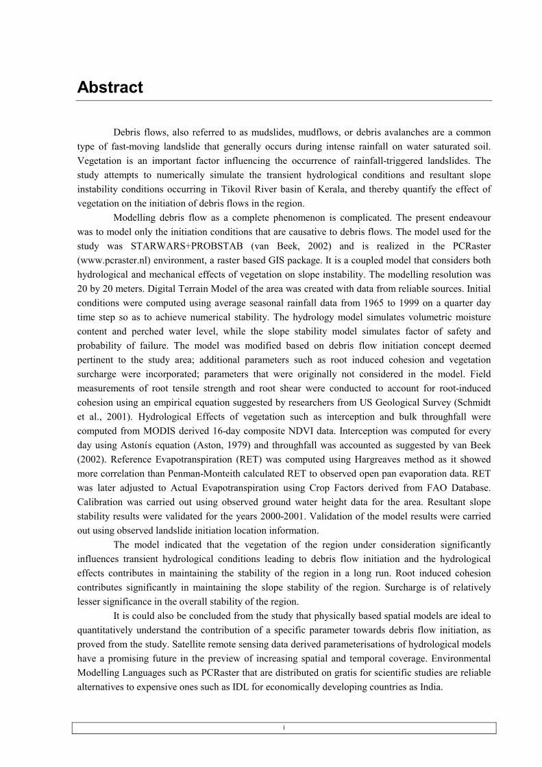
Debris flows, also referred to as mudslides, mudflows, or debris avalanches are a common type of fast-moving landslide that generally occurs during intense rainfall on water saturated soil. Vegetation is an important factor influencing the occurrence of rainfall-triggered landslides. The study attempts to numerically simulate the transient hydrological conditions and resultant slope instability conditions occurring in Tikovil River basin of Kerala, and thereby quantify the effect of vegetation on the initiation of debris flows in the region. Modelling debris flow as a complete phenomenon is complicated. The present endeavour was to model only the initiation conditions that are causative to debris flows. The model used for the study was STARWARS+PROBSTAB (van Beek, 2002) and is realized in the PCRaster (www.pcraster.nl) environment, a raster based GIS package. It is a coupled model that considers both hydrological and mechanical effects of vegetation on slope instability. The modelling resolution was 20 by 20 meters. Digital Terrain Model of the area was created with data from reliable sources. Initial conditions were computed using average seasonal rainfall data from 1965 to 1999 on a quarter day time step so as to achieve numerical stability. The hydrology model simulates volumetric moisture content and perched water level, while the slope stability model simulates factor of safety and probability of failure. The model was modified based on debris flow initiation concept deemed pertinent to the study area; additional parameters such as root induced cohesion and vegetation surcharge were incorporated; parameters that were originally not considered in the model. Field measurements of root tensile strength and root shear were conducted to account for root-induced cohesion using an empirical equation suggested by researchers from US Geological Survey (Schmidt et al., 2001). Hydrological Effects of vegetation such as interception and bulk throughfall were computed from MODIS derived 16-day composite NDVI data. Interception was computed for every day using Astonís equation (Aston, 1979) and throughfall was accounted as suggested by van Beek (2002). Reference Evapotranspiration (RET) was computed using Hargreaves method as it showed more correlation than Penman-Monteith calculated RET to observed open pan evaporation data. RET was later adjusted to Actual Evapotranspiration using Crop Factors derived from FAO Database. Calibration was carried out using observed ground water height data for the area. Resultant slope stability results were validated for the years 2000-2001. Validation of the model results were carried out using observed landslide initiation location information. The model indicated that the vegetation of the region under consideration significantly influences transient hydrological conditions leading to debris flow initiation and the hydrological effects contributes in maintaining the stability of the region in a long run. Root induced cohesion contributes significantly in maintaining the slope stability of the region. Surcharge is of relatively lesser significance in the overall stability of the region. It is could also be concluded from the study that physically based spatial models are ideal to quantitatively understand the contribution of a specific parameter towards debris flow initiation, as proved from the study. Satellite remote sensing data derived parameterisations of hydrological models have a promising future in the preview of increasing spatial and temporal coverage. Environmental Modelling Languages such as PCRaster that are distributed on gratis for scientific studies are reliable alternatives to expensive ones such as IDL for economically developing countries as India.

ii
Acknowledgements
I express my sincere thanks and gratitude to Dr. Cees J. van Westen and Prof. R.C Lakhera for being my first supervisors and lighting a way for me that is current in earth sciences. Words are not enough to express the gratitude to Dr. Rens van Beek for spending his valuable time in advising me all through the thesis work and direct me in every step towards achieving the goals. I thank Mr. G. Sankar for being my supervisor and especially in spending his time and efforts in the field with me and providing access to a plethora of data. Dr. Thw. van Asch, in spite of a busy schedule spent his valuable time on advising me, I thank him for his valuable comments right from the proposal stage and I hope I could do justice to the time that he has spent for me. I thank Drs. Dinand Alkema for motivating and guiding me to learn the fundamentals of dynamic modelling and especially for enabling me to acquire enough skills in PCRaster. I thank Dr. V. Hari Prasad, Programme Coordinator (HRA Courses), IIRS, for standing firm in his support to my research aspirations. Without his constant guidance and advises it would not have been possible to even envisage such a research work. My sincere thanks and gratitude is due to Dr. Paul. M. van Dijk, Programme Director and Assistant Professor, ITC for allowing me to return to ITC and carryout the modelling part of the study along side my supervisors and advisors. Thanks are due to Dr. V.K Dadhwal, Dean, IIRS for allowing me to pursue the course at the institute. The advices and directions provided by Dr. David G. Rossiter, Associate Professor, ITC and Dr. P.K Joshi, Scientist, FED, IIRS were of boundless value; I thank them, for the time and efforts that they put in providing me with insights into achieving my goals. I cannot forget the lengthy mails and telephonic discussions that I had with one of my very best friends, Ms. Shruthi B.V, IISc Bangalore, which developed further into many sections as dealt in the thesis. She was a constant motivation and support and I thank her for the same. Thanks and gratitude is due to Mr. Sam Varghese, JRF, IIRS for being my roommate and such a loving person who always took care of my needs whenever I needed. I also thank Mr. N.V Lele, JRF, IIRS for the intelligent suggestions and contributions of his in the thesis work. I thank Dr. M. Baba, Director, CESS for letting me work in the institution. I also thank Mr. Johan Mathai, Scientist, CESS for all the support that he provided while I was at the institution. My sincere thanks are due to Mr. B. Sukumar and Mrs. Ahalya Sukumar, Scientists, CESS for the valuable discussions that they had with me on my research topic. Thanks are due to Mr. S. Sidharthan, Scientist, CESS for providing me with the most crucial datasets for the study. The support provided by the Rubber Research Institute of India, Kottayam and Kurisumala Christian Monastery cannot be ignored. The climatic data sourced from these two institutions were crucial for the research and I thank them for providing me the data. I thank two of my friends, Mr. S. Devavrathan, Project Associate, CESS and Mr. Javed Malick, Student, M.Sc Geoinformatics in morally supporting me through the crucial phases of the project. Thanks are also due to Mr. Raju Francis, Mr. Sunil Sahadevan and Mr. Anil Antony, Range Officers, Kerala State Forests and Wildlife Department for being my friends and letting me relax even when I was in a hot seat. I also thank Mr. Asok Sekhar, M.Tech Student, IIRS and Mr. Prasanth Narayanan, JRF, SACON for being my friends.

iii
Table of contents List of Tables................................................................................................................................................. v List of Equations.......................................................................................................................................... vi List of Figures ............................................................................................................................................. vii 1. Introduction .................................................................................................................................................. 1 1.1. Debris Flows............................................................................................................................ 1 1.2. Problem Statement................................................................................................................... 2 1.3. Aim and Objectives ................................................................................................................. 3 1.3.1. Research Questions.......................................................................................................... 3 1.3.2. Research Hypothesis........................................................................................................ 3
2. Literature Review......................................................................................................................................... 4 2.1. De br i s Fl ow - Definition ......................................................................................................... 4 2.2. Overview of Research Works.................................................................................................. 5 2.3. Debris Flow Studies in India ................................................................................................... 5 2.3.1. Debris Flow studies in Kerala ......................................................................................... 6
2.4. Modelling................................................................................................................................. 7 2.5. Debris Flow Components ........................................................................................................ 9 2.5.1. Contributing Factors ........................................................................................................ 9
2.6. Debris Flow Initiation............................................................................................................ 10 2.7. Effect of Vegetation .............................................................................................................. 12 2.7.1. Hydrological Effects...................................................................................................... 12 2.7.2. Mechanical Effects ........................................................................................................ 13
2.8. Debris Flow Modelling.......................................................................................................... 14 2.8.1. Scale Consideration ....................................................................................................... 15 2.8.2. Choice of the model....................................................................................................... 15
2.9. The PCRaster Software ....................................................................................................... 16 3. Study Area................................................................................................................................................... 18 3.1. Kerala .................................................................................................................................... 18 3.2. The Tikovil River Basin ........................................................................................................ 20 3.2.1. Physiography ................................................................................................................. 20 3.2.2. Drainage......................................................................................................................... 21 3.2.3. Geology.......................................................................................................................... 23 3.2.4. Soil................................................................................................................................. 23 3.2.5. Climate........................................................................................................................... 25 3.2.6. Landuse.......................................................................................................................... 26 3.2.7. Debris Flows.................................................................................................................. 29
4. Materials and Methods .............................................................................................................................. 34 4.1. The Model ............................................................................................................................. 34 4.1.1. ST ARWARS - The Slope Hydrology Model ............................................................... 34 4.1.1.1. Effects of Vegetation ............................................................................................. 36
4.1.2. PROBST AB - The Slope St ability Model .................................................................... 37 4.2. The Data ................................................................................................................................ 42 4.3. Methods ................................................................................................................................. 43 4.3.1. Choice of Modelling Resolution ................................................................................... 44 4.3.2. Choice of Model Validation Period and Time-step....................................................... 44

iv
4.3.3. Data Preparation ............................................................................................................ 44 4.3.3.1. Field Work............................................................................................................. 44 4.3.3.2. Locating Debris Flow ñ Old and Recent ............................................................... 47 4.3.3.3. Landuse.................................................................................................................. 47 4.3.3.4. Soil Thickness........................................................................................................ 48 4.3.3.5. Soil Type................................................................................................................ 48 4.3.3.6. Field Verification................................................................................................... 49
4.4. Model Parameterisation......................................................................................................... 50 4.4.1. Rainfall Time-series ...................................................................................................... 51 4.4.2. Potential Evapotranspiration Time-series...................................................................... 52 4.4.3. Interception, BT Coefficient, Effective Rainfall and Soil Erc Time-series Maps.......... 53 4.4.4. Root Induced Cohesion (Map) and Surcharge (Scalar Value) ...................................... 54 4.4.5. DT M - Map ................................................................................................................... 56 4.4.6. Landuse, Soil Type and Soil Thickness ñ Maps............................................................ 56
4.5. The Model Run...................................................................................................................... 59 4.5.1. The Model Calibration .................................................................................................. 60 4.5.2. Model Validation........................................................................................................... 60
5. Results and Discussion................................................................................................................................ 62 5.1. Parameterisation .................................................................................................................... 62 5.1.1. Rainfall .......................................................................................................................... 62 5.1.2. Potential Evapotranspiration ......................................................................................... 63 5.1.3. Interception.................................................................................................................... 64 5.1.4. Effective Rainfall and Bulk Throughfall Time-series Maps ......................................... 67 5.1.5. Soil Erc Time-series Maps.............................................................................................. 68 5.1.6. Root Induced Cohesion and Surcharge.......................................................................... 71 5.1.7. Soil Thickness Map ....................................................................................................... 73
5.2. Model Run ............................................................................................................................. 74 5.3.1. STARWARS Results..................................................................................................... 75 5.3.2. Sensitivity of STARWARS........................................................................................... 76 5.3.3. PROBSTAB Results...................................................................................................... 82 5.3.3.1. Probability of Failure............................................................................................. 88
5.3.4. Area Validation ............................................................................................................. 89 5.3.5. Sensitivity of PROBSTAB ............................................................................................ 89
6. Conclusion and Recommendations............................................................................................................ 95 6.1. Results from the perspective of research objectives ............................................................. 95 6.2. Results from the perspective of research questions............................................................... 95 6.3. Hypothesis Validity ............................................................................................................... 97 6.4. Summary................................................................................................................................ 97 6.5. Limitations............................................................................................................................. 99 6.6. Recommendations................................................................................................................ 100
Glossary.............................................................................................................................................................. 101 References:......................................................................................................................................................... 103 Appendix 1: ........................................................................................................................................................ 111 Appendix 2: ........................................................................................................................................................ 113 Appendix 3: ........................................................................................................................................................ 114 Appendix 4: ........................................................................................................................................................ 115 Appendix 5: ........................................................................................................................................................ 117

v
List of Tables
Table 1: Basic Factors considered as contributing to Landslides ........................................................... 9 Table 2: Factors Controlling Occurrence and Distribution of Shallow Landslides ................................ 9 Table 3: Drainage Characteristics of the Study Area ............................................................................ 21 Table 4: Major Soil Types in the Study Area........................................................................................ 23 Table 5: Available Meteorological Parameters for the nearest Met Station ......................................... 25 Table 6: Characteristics of debris flows in the study area (based on field measurements) .................. 31 Table 7: Model in & output of ASTONís, STARWARS, Effective Degree of Saturation and
PROBSTAB Models...................................................................................................................... 41 Table 8: Data, Sources and Use............................................................................................................. 42 Table 9: Crop Factors for computing Actual Evapotranspiration ......................................................... 48 Table 10: Soil Thickness Class, Thickness Values used and Area Covered......................................... 48 Table 11: Seasonal Totals of a representative hydrological normal year and leap year ....................... 51 Table 12 (a), (b) & (c): Soil Hydrological and Mechanical Properties used ........................................ 59 Table 13: Soil Type, Depth, Slope and Landuse characteristics of Flow Initiation Locations in 2000
and 2001 ........................................................................................................................................ 61 Table 14: Root Sample - Diameters and Tensile Strength .................................................................... 71 Table 15: Minimum, Maximum, Average and Standard Deviation of Predicted Water Levels
(considering vegetation effects) at the 2000 and 2001 Flow Initiation Locations and Soil Depths at the locations............................................................................................................................... 80
Table 16: Simulated Slope Hydrology for July 8th 2001 at the Flow Initiation Locations of 2001, with and without considering vegetation effects ................................................................................... 80
Table 17: Minimum, Maximum, Average and Standard Deviation of Safety Factor (considering vegetation effects) at the 2000 and 2001 Flow Initiation Locations ............................................. 87
Table 18: Probability of Failure at Debris Flow Initiation Locations of 2000 and 2001...................... 89 Table 19: Area comparison between derived P(FS<=1) and Landslide Hazard Zones based on the map
of CESS ......................................................................................................................................... 89

vi
List of Equations
Relative Degree of Saturation: [1]......................................................................................................... 35 Astonís Equation for Canopy Interception: [2] ..................................................................................... 36 Von Hoyningen-Huene Equation for Maximum Canopy Storage: [3].................................................. 36 Leaf Area Index: [4] .............................................................................................................................. 36 Fractional Vegetation Cover: [5]........................................................................................................... 36 Bulk Throughfall Coefficient: [6] ......................................................................................................... 37 Factor of Safety: [7]............................................................................................................................... 37 Effective Degree of Saturation: [8] ....................................................................................................... 37 Variable Performance: [9] ..................................................................................................................... 38 Mean Factor of Safety: [10] .................................................................................................................. 38 Cumulative Variance of Factor of Safety: [11] ..................................................................................... 38 Z score assuming normal distribution: [12]........................................................................................... 38 Standard Deviation of Factor of Safety: [13] ........................................................................................ 39 Coefficient of Variation of Factor of Safety: [14]................................................................................. 39 Logarithmic term of Factor of Safety: [15] ........................................................................................... 39 Z score assuming logarithmic distribution: [16] ................................................................................... 39 Porosity: [17] ......................................................................................................................................... 49 Extraterrestrial Solar Radiation: [18] .................................................................................................... 52 Hargreaves Equation for Evapotranspiration: [19] ............................................................................... 53 Root Induced Cohesion: [20]................................................................................................................. 55 Root Shear Correction Parameter for Root Induced Cohesion: [21]..................................................... 55 Van Genutchen Equation for Relative Degree of Saturation: [22] ....................................................... 56 Model implementation of Effective Rainfall: [23]................................................................................ 67 Model implementation of Soil Evapotranspiration: [24] ...................................................................... 68

vii
List of Figures
Figure 1: Morphology of Debris Flow .................................................................................................... 5 Figure 2: Model Development Cycle ...................................................................................................... 8 Figure 3: Initiation of a Soil Slip Debris Flow...................................................................................... 11 Figure 4: Initiation of Debris Flow according to Blijenberg................................................................. 11 Figure 5: Hydrological (a) and Mechanical (b) effects of Vegetation on Slope Stability .................... 14 Figure 6: Location Map......................................................................................................................... 18 Figure 7: Digital Terrain Model ............................................................................................................ 22 Figure 8: Stream Order, Figure 9: Lithology and Figure 10: Soil Types .............................................. 24 Figure 11: Rainfall and Rainy Days in the Study Area (Station: Kurissu Mala Monastery, Year: 2000 -
2001).............................................................................................................................................. 26 Figure 12: Landuse (Photographs) ........................................................................................................ 27 Figure 13: Landuse Map........................................................................................................................ 28 Figure 14: Remnants of old slides ......................................................................................................... 29 Figure 15 (a & b): Old (before 2001) and New (2005) Debris Flows in Rubber Plantation ................ 30 Figure 16: The Crown of June 5th 2005 Debris Flow........................................................................... 30 Figure 17: Cross section of a hollow..................................................................................................... 31 Figure 18 & Figure 19: Landslide Population overlaid on Landuse Map and Stream Order Map ....... 32 Figure 20: Debris Flow: An Anatomy................................................................................................... 33 Figure 21: Lanslide Hazard Zonation of the Study Area ...................................................................... 33 Figure 22: Coupled Model of STARWARS + PROBSTAB................................................................. 40 Figure 23 (a & b): Contour Bunding & Drainage Alteration, and Surface Detention .......................... 45 Figure 24: A typical hollow................................................................................................................... 45 Figure 25: Root Anchoring to Bed Rock Figure 26: Soil Thickness Verification............................ 50 Figure 27: Variation of derived daily rainfall in a normal year and a leap year and the respective
percentages of each dayís rainfall from the seasonal total ............................................................ 52 Figure 28: Angle of Shear ..................................................................................................................... 55 Figure 29 (a, b, c, d & e): Relationship between Matric Suction and Relative Degree of Saturation
calculated with Van Genutchen equation and Farrel and Larson equation for the Soil Units ...... 58 Figure 30: Rainfall of Hydrological Years in the study area from 1965 to 1995.................................. 62 Figure 31: Daily Variability of Rainfall in Hydrological Leap year and Normal year based on 2000-
2001 data........................................................................................................................................ 63 Figure 32: Potential Evapotranspiration of 2000-2001 and hypothetical years .................................... 64 Figure 33: Comparison of Fractional Vegetation Cover computed using different methods ............... 65 Figure 34: Interception at two locations for the calendar year 2001..................................................... 65 Figure 35: Average Monthly Interception Maps ................................................................................... 66 Figure 36: Average Annual Bulk Throughfall Coefficient ................................................................... 69 Figure 37: Soil Evapotranspiration of 7th and 8th July 2001................................................................ 70 Figure 38: Root Diameter-Root Tensile Strength Relationship ............................................................ 71 Figure 39: Root Counts at various Soil Depths ..................................................................................... 72 Figure 40: Root Induced Cohesion as it varies with Soil Depth for each Soil Type............................. 72 Figure 41: Root Induced Cohesion........................................................................................................ 73 Figure 42: Soil Thickness Map.............................................................................................................. 74

viii
Figure 43: Relationship between Observed and Predicted Water Levels for 2005............................... 75 Figure 44: Predicted Maximum Water Levels for the Hydrological Years of 2000 and 2001, with and
without hydrological effects of vegetation .................................................................................... 78 Figure 45: Predicted Maximum Effective Degree of Saturation for the Hydrological Years of 2000
and 2001, with hydrological effects of vegetation ........................................................................ 79 Figure 46 (a & b): Water Levels predicted for two Debris Flow Initiation Locations each, considering
Vegetation Effects for the years 2000 & 2001 .............................................................................. 81 Figure 47 (a) & (b): Overall Stability of the study area in 2000 and 2001, considering vegetation
effects ............................................................................................................................................ 83 Figure 48: Daily Variations of Safety Factor in 2000 as visualized in PCRaster ................................. 84 Figure 49 (a & b): Daily Variation of Safety Factor for 2000 and 2001, considering Vegetation Effects
....................................................................................................................................................... 85 Figure 50 (a & b): Daily Variation of Safety Factor for 2000 and 2001, without considering
Vegetation Effects ......................................................................................................................... 86 Figure 51 (a) & (b): Overall Stability of the study area in 2000 and 2001, without considering
vegetation effects........................................................................................................................... 91 Figure 52 (a) & (b): Probability of Failure for areas with FS<=1 in 2000 and 2001............................ 92 Figure 53: Sensitivity of Slope Stability to contributing parameters .................................................... 93 Figure 54: Contribution of Slope Stability Parameters to variance....................................................... 94

Effect of Vegetation on Debris Flow Initiation - Conceptualisation and Parameterisation of a Dynamic Model for Debris Flow Initiation in Tikovil River Basin, Kerala, India, using PCRaster
1
1. Introduction The captivating profile of cascading rivers and high rising mountains in the twilight has evoked
romanticism in poets as great as Shelly. Little would have been known to him that there are complex processes involved in the shaping of these cascades and the profiles that instigated the poet in him. Landscapes are dynamical earth surface systems containing not only objects, but also stores of energy and matter, maintained by processes of growth, decay, flow, and transformation (Thomas, 2001).
These movements and processes were in action ever before human kind evolved on earthí surface; constant destruction (weathering and erosion) and rebuilding (rejuvenation) are those that have shaped the earth. The geophysical events that were part of the natural evolutionary system of the earth turned into ënatural hazardsí when the human system started interacting with it. The human system itself was subjected to significant transformations, where the concept of work and hence of social division of work, production relations and economical ñ political systems appeared. These transformations and their links to the natural system have served as templates of the dynamics of natural hazards and therefore, of natural disasters (Alcantara-Ayala, 2002). According to EM-DAT (2005b) during the period of 1994-2003 natural hazards caused as much as 680176 Million US Dollars damage globally. Of the 3055 disasters reported and stored in the Emergency Event Database for the same period 186 are landslides and avalanches and the events killed as many as 8679 people. Estimated damage from these events are up to 427 million US Dollars (EM-DAT, 2005b). All the datasets provided in EM-DAT has its clear limitations; only those natural hazards that significant based on the criteria laid out by EM-DAT are only provided. Those landslides that fulfil any one of the criteria of having 10 people killed, 100 people affected, created a havoc requiring international assistance or declaration of state of emergency are reported in EM-DAT. The actual number of landslides that affected human life during the period would have been far more than this number, let alone those events that occur without being noticed or affecting human society.
Landslides in its strict sense are relatively rapid downslope movement of soil and rock, which takes place characteristically on one or more discrete bounding slip surfaces, which define the moving mass (Hutchinson, 1988). As single hazardous events, they may cause only localized and minor damage in comparison with earthquakes or floods. As human populations expand and occupy more and more of the land surface, mass wasting processes become more likely to affect humans. Changes obligated by humans on landuse/landcover affects the slope stability of a hilly/mountainous terrain. The changes not only affect the effective precipitation that reaches the earthís surface and resultant runoff but as well influences the cohesion of the soil and root reinforcement provided by the vegetation cover. To approach from a subject expertís words, ì The loss of vegetation cover, either grass or forest, by overgrazing, fire or clear-cut logging not only alters the hydrologic conditions of a slope but is widely believed to promote rapid run-off and erosion, and to increase the possibility of slides and debris flowsî (Varnes, 1984).
1.1. Debris Flows
Debris flow is a type of mass movement/landslide. They are particularly dangerous to life and property because of their high speeds and the sheer destructive force of their flow (USGS, 2000). Often initiated by shallow landslides, they are the primary agent of landscape evolution and the dominant denudational process in humid forested areas (Iida, 1999). The debris flow system is more robust in mountainous terrains as the gradient of the terrain enables to gain disastrous momentum. They affect the land quality by resulting in intense soil loss as land managers struggle to conserve the soil. Debris flows

Effect of Vegetation on Debris Flow Initiation - Conceptualisation and Parameterisation of a Dynamic Model for Debris Flow Initiation in Tikovil River Basin, Kerala, India, using PCRaster
2
from many different sources can combine in channels, where their destructive power may be greatly increased. In the Himalayan belt they are called ëChoesí and ëRaoís (Juyal, 2000). In Kerala in the local vernacular (Malayalam), they are known as ëUrul Pottalí. Larger pebbles and cobbles characterize the Choes of Himalayan belt whereas loose sand, silt and clay characterize those along the Western Ghats. The characteristic pattern of these phenomena is the swift and sudden down slope movement of highly water saturated overburden containing a varied assemblage of debris material ranging in size from soil particles to huge boulders destroying and carrying with it every thing that is lying in its path (Sankar, 2005).
1.2. Problem Statement
Landslides are increasingly a concern in India. Much of the increase in landslide activity is observed along dynamic regions in terms of landuse/landcover. Though India statistically improved in terms of forest cover (F.S.I, 2001), the fact is undisputable that many of the forested areas of the country are under tremendous pressure from degradation and deforestation. Conditions of the forests of Kerala are not different. Studies on a 40000 Km2 area in the state estimate that the annual rate of deforestation is 1.16%. The dense forest has shrunk by 19.5% or at an annual rate of 0.8%, and the open forest has decreased in area by 33.2%, or an annual rate of 1.5%. As a result, areas have increased under degraded forest (26.64%), grasslands (28.73%), plantations (6.78%), and agriculture (11.15%) (Jha et al., 2000). The increase in agricultural land and plantations implies that the causes of these changes are anthropogenic in origin.
Continued disturbance and changes are clear and present a danger, as Kerala being the second most densely populated state of the country. Moreover, 40% of the state lies in the most prominent orographic feature of peninsular India, The Western Ghats. Thus, the state is prone to landslides due to its geomorphic setting. The most common landslides are debris flows (CESS, 2000). Floods and landslides killed almost a 100 people in different parts of Kerala and caused damages to the tune of Rs 50 crore in 2005 (Ajith, 2005). The Emergency Event Database lists two major landslide events in the state, one in 1992 and the other in 2001 reported of killing 60 and 55 people respectively (EM-DAT, 2005a). For a period from 1975 to 1995, it is estimated that about a 100 people have been killed of landslides and about 600 families rendered homeless along the Western Ghats (Thakur, 1996). The available statistics itself indicates the insufficiency of research into the field. Many minor events that cause damages in a localized manner are unrecorded. The damage to property and loss of lives are enormous when cumulative figures are taken of all the landslides occurring in a given period.
Disturbed by the highland settlers and the extensive rubber, tea and cardamom plantations in the hilly terrain of the state, the slopes once relatively stable are increasingly seen to be unstable. The removal of natural vegetation from the slopes, exposing them to heavy rainfall (annual average of 3000 mm) and inducing monoculture has aggravated the situation. The situation is particularly evident in the upper reaches of Idukki and Kottayam districts of the state. A study by the Center for Earth Science Studies (Trivandrum, Kerala) identified that ëamong landuse types the areas with degraded natural vegetation shows maximum slide intensityí (Thampi et al., 1998a). This necessitates research to quantify the influence of vegetation on slope stability in the region.
Vegetation cover is an important factor influencing the occurrence and movement of rainfall-triggered landslides, and changes to vegetation cover often result in modified landslide behaviour (Glade, 2003). There have been a number of attempts in dynamic spatial modelling of the effects of landuse/landcover on debris flows (van Asch et al., 1999; van Beek, 2002). Most of the studies consider the effect of change in vegetation cover on debris flows and landslides in terms of the effective rainfall that reaches the earthís surface. However, studies elsewhere have identified several other effects of vegetation

Effect of Vegetation on Debris Flow Initiation - Conceptualisation and Parameterisation of a Dynamic Model for Debris Flow Initiation in Tikovil River Basin, Kerala, India, using PCRaster
3
on soil erosion in general and landsliding in particular (Lancaster and Grant, 1999). The present study utilizes a physically based spatial, deterministic, dynamic model to simulate the manifestations of vegetation effect on debris flow initiation.
1.3. Aim and Objectives
The study aims at quantification of the hazard of debris flow initiation considering vegetation effects, driven by the need to understand the risk following increased population pressure, in the upper catchment of Tikovil River that flows through Idukki and/or Kottayam districts of Kerala, using a physically based spatial modelling approach. The more specific objectives are:
• To conceptually understand the effects of vegetation on debris flow initiation. • To quantify the hazard of debris flow under present land use conditions using a calibrated and
validated physically-based model. o To run the model with and without considering vegetation parameters as a controlling
factor. • To determine the relative importance of the hydrological and mechanical effects of vegetation on
slope stability through: o Assessing the relative changes in the simulated results and o Sensitivity analysis of the model towards different slope stability parameters.
1.3.1. Research Questions
• What are the parameters required for simulating debris flow initiation? • How can these parameters be most optimally obtained for the study area? • Which of these parameters are the most crucial in the initiation of debris flow in the study area? • Is the data available in Kerala sufficient to run an exhaustive debris flow initiation model? • Should a simpler physically based dynamic model be used owing to data deficiency? • Is deterministic modelling the best solution for studying debris flow initiation using a medium scale
data set and literature derived parametric values? • How to parameterise root induced cohesion for debris flow initiation modelling? • How to carry out a sensitivity analysis for the model derived results and validate the hypothesis?
1.3.2. Research Hypothesis
• Physically based spatial models provide reasonable quantification of the effects of vegetation on debris flow initiation even in a data deficient condition.
• Debris flow initiation at a given location is highly sensitive to the prevailing vegetation conditions in the region, especially to root induced cohesion and surcharge.

Effect of Vegetation on Debris Flow Initiation - Conceptualisation and Parameterisation of a Dynamic Model for Debris Flow Initiation in Tikovil River Basin, Kerala, India, using PCRaster
4
2. Literature Review
2.1. De bris Flow - De fi ni ti on
Based on various considerations, researchers have defined debris flows in many ways, though it is difficult to address the entire complexity of the phenomena within a tight bracket definition. Debris Flows (also known as Mud-flow) are destructive events caused when eroded and other loose geological materials are mixed with water to the point where they begin to move down a gradient as one semi-cohesive mass, usually defined where sediment concentrations are greater than 60% by volume or 80% by weight (Vallance and Scott, 1997). Researchers state that snow melt, Glacial Lake Outbreaks and volcanic ash when saturated can as well create debris flows (Daag, 2003; Das, 1995; Kniveton et al., 2000; Malet et al., 2004).
The mo s t accepted of all definitions is that by Varnes (1978); 'F l o w s are rapid mo v e me n t s of material as a viscous mass where inter-granular movements predominate over shear surface movements. These can be debris flows, mudflows or rock avalanches, depending upon the nature of the material involved in the mo v e me n t ' (Varnes, 1978). Hi s definition includes both the constituent ma t e r i a l size and the speed of movement of the material. He even differentiates debris flows from mudflows using Shroderís (1971) criteria of '20 to 80% mat e r i al above 2 mm size' (Varnes, 1978). USGS provides a functional definition stating that 'Debris flows (also referred to as mudslides, mudflows, or debris avalanches) are a common type of fast-moving landslide that generally occurs during intense rainfall on water-saturated soil. They usually start on steep hillsides as soil slumps or slides that liquefy and accelerate to speeds as great as 35 miles per hour or moreí (Gori and Burton, 2003).
Often the word ëtorrentí is used to describe debris flows. The definitions technically addresses the same phenomena, only possible difference being, the term ëdebris flowí defines the phenomena whereas the term ëtorrentí describes the milieu of occurrence. The terms are complimentary and not mutually exclusive. A report brought out by Government of Nepal defines debris torrents as a channel that involves rapid movement of water charged soil, rock and organic material, down steep river characterized by (1) a funnel shaped watershed area, (2) a debris source, (3) a narrow gorge and (4) debris fan [HMG, Nepal (1987) in (Das, 1995)].
A debris flow system can fundamentally be divided into three zones: a source area, a transport zone (confined or unconfined) and a deposition zone (Figure 1). The source of debris flow is often defined as from ëhollowsí that are topographic depressions depicted by concave contours (Melelli and Taramelli, 2004). These swales continuously supply debris to stream channels and act as slope failure hotspots by converging infiltration leading to perched groundwater tables. The transportation zone of debris flow is often confined to existing gullies. Often mountain torrents are prone to episodic debris flow events (Arattano and Franzi, 2004). However, debris flows can occur in unconfined slopes as well. The debris deposition zones are easily recognizable in the field because of the typical morphology of the two latter zones: a long and small, ribbon-like channel bordered by lateral levees which meet downslope in a lobate and tongue-shaped terminal deposit [Jager, (2001) in (Naldini, 2004)]. They resemble the cone-shaped alluvial fans; however, they may be different when a debris flow coalesces with a stream or river in the valley, which will wash off the fan eventually.

Effect of Vegetation on Debris Flow Initiation - Conceptualisation and Parameterisation of a Dynamic Model for Debris Flow Initiation in Tikovil River Basin, Kerala, India, using PCRaster
5
Figure 1: Morphology of Debris Flow
[Adopted from (CCI&AD, 2003) and modified]
2.2. Overview of Research Works
Liua and Lei (2003) provides a brief description of research on debris flows since early 20th century. Perhaps the most remarkable contribution to landslide studies appeared in 1978 in the Special Report 176 (Schuster and Krizek, 1978) on Landslide Analysis and Control published by the National Academy of Sciences, US, wherein David J. Varnes contributed a classical chapter on Slope Movement Types and Processes. Having a clear definition to stick to, several geomorphologists worked on the physics of debris flow and several others addressed it from the hazard perspective.
It was only in 1960s that systematic studies on debris flows in laboratories began. The initial attempts were to apply three simple fluid models to debris flow namely ñ Newtonian Flow, Bingham Fluid Flow and Dilatant Grain Shearing Flow (Rickenmann, 1999). Results from various such studies were reviewed and published by Iverson (1997). Once that the physical processes involved became clear, including the several key components of flow initiation and runout, substantial number of researchers turned their attention to modelling the phenomena in a digital environment.
2.3. Debris Flow Studies in India
Landslide research works in India received deserving attention in the year 1994 through the report presented by the Ministry of Agriculture, Govt. of India, to the world conference on the IDNDR held in Japan. Rao (1989) identifies five major regions in India that are susceptible to landslides:
1. Western Himalayas (Uttar Pradesh, Himachal Pradesh and Jammu & Kashmir)

Effect of Vegetation on Debris Flow Initiation - Conceptualisation and Parameterisation of a Dynamic Model for Debris Flow Initiation in Tikovil River Basin, Kerala, India, using PCRaster
6
2. Eastern & North Eastern Himalayas (West Bengal, Sikkim and Arunachal Pradesh) 3. Naga ñ Arakkan Mountain belt (Nagaland, Manipur, Mizoram, Tripura) 4. Plateau Margins in the Peninsular India and Meghalaya in the NE India. (Rao, 1989) It is seen that considerable work has been done by various national agencies in the Himalayan
region, while limited attention has been paid to the Western Ghats region (Thampi et al., 1998a). The lack of stress on southern states may be attributed to the fact that slides in Ghats are smaller compared to those in the Himalayan region.
Even though considerable number of landslide researches have happened in India most of them focus on deep-seated slides; slides such as flows and creep having differential movement rates receive little attention owing to the complexity involved in discerning the underlying processes. There are only few research articles that are of Indian origin which could be found through internet and library search pertaining to debris flows and torrents. This shows a research gap in disaster related research works in the country. The reason for this gap may be attributed to focus on conventional research orientation or may be because many research works are not reported nationally or internationally.
Since the colonial period, several studies have been conducted in India on the mountain torrents of Himalayas that frequently experience debris flows. L.B. Holland did one of the earliest known studies on torrents in Siwaliks as early as in 1928. He clearly expresses the ëproblems of land degradation and its consequences as manifested through flash floodsí. British government, understanding the requirement of legislation to prevent uncontrolled abatement of forests and the consequent land degradation and erosion passed the Punjab Land Preservation (CHOS) Act 1900. Gorie (1946), Bajwa (1983), Mishra and Sarin (1987) are few others who looked into the issue over years (Katiyar and Mittal, 2000). Katiyar and Mittal (2000) identifies the research needs for torrent control. Citing several research documents and governmental plans, they conclude the requirement of comprehensive research in the field. The fact is much more evident from the words of Juyal (2000), wherein he cites an anonymous authorís words from 26th edition of Indian Agriculture in brief (1995), published by Ministry of Agriculture, who accounts 2.73 million hectares of land as affected by torrent damage (Juyal, 2000). He further states ëbank cutting followed by debris deposition has converted good productive agricultural and forest lands to barren and infertile fieldsí.
Attempts to assess risk zones of soil erosion due to torrents utilizing remote sensing data sets were attempted in IIRS in 1995 (Bhan et al., 1995). The study lays down a methodology to understand and comprehend the torrent induced soil erosion and consequent damage to agricultural lands. Rao et al., (1995) laid down a methodology to assess changes in extent of torrents using remote sensing data sets. The work concludes that torrents tend to increase in width by somewhere between 50 meters to 719 meters and length over years. Torrents in the region tend to swell between 75 to 150 meters over a period of 24 years (1965 to 1989) (Rao et al., 1995).
2.3.1. Debris Flow studies in Kerala
With the exception of the coastal district of Alappuzha, landslides and especially debris flows are prevalent in 13 of the 14 districts of Kerala. Landslide studies in Kerala are carried out as a thrust research subject by the Center for Earth Science Studies (CESS) in Trivandrum. Other institutions that conduct landslide related research in the state are the National Transportation Planning and Research Center (NATPAC) Trivandrum, the Center for Water Resources Development and Management (CWRDM), Kozhikodu and the National Institute of Technology (former REC), Kozhikodu.
Studies in CESS are focussed towards mapping landslide hazard zones and are mostly post event evaluation reports for governmental purposes. One of the most phenomenal works of CESS is the one titled, ëEvaluation study in terms of landslide mitigation in parts of Western Ghats, Keralaí, which does detailed

Effect of Vegetation on Debris Flow Initiation - Conceptualisation and Parameterisation of a Dynamic Model for Debris Flow Initiation in Tikovil River Basin, Kerala, India, using PCRaster
7
observations of the various contributing factors to landsliding (Thampi et al., 1998a) in a 750 km2 area covering the districts of Kottayam and Idukki. The study evaluates the area using a Qualitative Zonation approach based on assigning relative weightings for discerned causative parameters such as Slope, Soil Thickness, Landuse, Relative Relief, Drainage, Landform and Rainfall.
Though a detailed geotechnical survey of the soils in the region was carried out, the data was ruled out from being we i ght e d for the zonation, citing the fact; 's i n c e the physical properties of soil from the entire area sampled gives a rather uniform low safety factor in wet condition and a high safety factor indicating stability in natural dry state; this parameter could be of limited application in regional hazard zonation study' (T hampi et al., 1998a). The report opines that the mo s t commonly occurring type of landslide in Kerala is Debris Flows. The study also compiles firsthand field description of several debris flow events that happened in Kerala. This being the first of its kind in the state the study was a significant contribution in terms of providing a pragmatic methodology to be later applied in several other regions. The study also describes the significant characteristics of debris flows that are prevalent in the state and observes that ëmajority of mass movements have occurred in steep slopes (+ 20°) in the highlandí (Thampi et al., 1998a).
Another study carried out in Kerala states that the action of groundwater movement during the monsoon season is the major causative factor of repeated landslide occurrence in Kullumala area of Palakkad District (Earnest et al., 1995). Possible relationship between structurally weak zones and landslide prone areas are reiterated by the observations made during a reconnaissance survey carried out by Geological Survey of India along the Wayanad Plateau in 1984 (Muraleedharan, 1995). The complex interaction between these structural trends and inherently unstable zones (topographically) during periods of high precipitation renders the regolith vulnerable, by surplus water resulting in very high pore pressures. Idukki district of Kerala is identified as one of the most vulnerable area by several authors and so is the hilly regions of Kottayam [Krishnanath et al., (1984) and Ramachandran, (1985) in (Thampi et al., 1998a)]. Analyzing the causative reasons of debris flows that occurred in Koodaranji in Koyilandi Taluk of Kozhikodu district, Sankar (1991) opines; ì During high rainfall infiltration is high due to blockage of drainage network on slopes by contour bunding. The absence of provision for draining of excess storm water was the main reason for failureî (Sankar, 1991).
NATPAC identified disaster prone zones along the hill roads of Western Ghats. CWRDM has carried out investigations in areas near Lakkidi in Kozhikodu district and suggested surface drainage correction and structural measures like buttressing to prevent sliding (Narasimha Prasad et al., 1995). Majority of the work was carried out using a stochastic models and no work could be identified which tried to utilize a physically based dynamic model for understanding and quantifying the causative parameters. As the research intents to quantify the phenomenon using a physically based dynamic model, a critical synthesis of models and modelling procedure follows. The relative advantages of physically based dynamic models are described in brief.
2.4. Modelling
Models are fundamentally a hypothesis. They are many a times only a little more than speculation. However, often scientific community tend to differentiate models, hypothesis and speculations, and consider speculations as not a valid part of scientific methodology (van Loon, 2004). Models are classically defined as a representation of reality; not real because models represent those perceptions of human kind of the object/subject being modelled. Models of the landscape are almost always representations in miniature even though the representation is physical (an analogue model) or in mathematical equations (Karssenberg,

Effect of Vegetation on Debris Flow Initiation - Conceptualisation and Parameterisation of a Dynamic Model for Debris Flow Initiation in Tikovil River Basin, Kerala, India, using PCRaster
8
2002). Owing to the complexity and dynamic nature of geomorphic processes, it is too difficult and often expensive to create laboratory scaled models and conduct research on the same. Computer models are a vi a b l e solution for process studies as they provide the capability of 'spatial dynami c modelling' ; spatial refers to the geographic domain and dynamic refers to the changes over time (Karssenberg, 2002).
Models for landscape process studies should ideally be open entities that can be modified for applications specific to the study being carried out. This demands a process flow for model building. Karssenberg (2000) quotes Jorgensen (1988) to identify the sequence of procedural steps involved in modelling (Figure 2): 1. Model Structure Identification, involving the selection of the processes governing the behaviour of the
system to be modelled, and the mathematical representation of these processes. 2. Programming the model, involving the conversion of the mathematical representation of the processes to
a computer programme 3. Estimation of appropriate values of input variables and parameters using field data, which can be done
by upscaling and/or inverse modelling. Upscaling includes various scaling methods needed to change data to appropriate input values and parameters as required by the model. Inverse modelling is a means to estimate inputs and parameters of a model by comparison of a set of outputs of a model with measurements of these outputs.
4. Validation ñ Assessing the quality of the predictions provided by a model is called validation.
Figure 2: Model Development Cycle
[After (Karssenberg, 2002)]

Effect of Vegetation on Debris Flow Initiation - Conceptualisation and Parameterisation of a Dynamic Model for Debris Flow Initiation in Tikovil River Basin, Kerala, India, using PCRaster
9
The process flow thus demands a clear understanding of various contributing factors of the process that is being modelled, in this specific case, the contributors to debris flow initiation. It is not yet possible to successfully replicate these natural multi-dimensional geomorphological systems in computer form, although considerable progress has been made in isolating many of the variables involved (Brunsden, 1999). Modelling is a complex procedure demanding multidisciplinary inputs. Brunsden (1999) provides a comprehensive listing of several aspects that needs to be considered by a geomorphologist in evaluating a model.
2.5. Debris Flow Components
A debris flow system theoretically has three components: initiation, transportation and deposition. All the three are largely controlled by the supply of water to the system. Ellen (1988) identifies 4 sequential phases towards the development of soil slip/debris flows, they being (1) movement of water to the site of failure, (2) failure of the soil mantle by sliding, (3) mobilization of the soil slip as a debris flow and (4) travel of the debris flow (Ellen, 1988). The present study limits its scope to understanding the initiation process, i.e, movement of water to the site of failure and failure of the soil mantle by sliding.
2.5.1. Contributing Factors
It is often difficult to discern the actual factors that initiate debris flow events. As observed by Crozier (1986) in va n Beek (2002), 't h e intrinsic factors change mo s t of the times only gr adually over time and can be considered as preparatory factors whereas the extrinsic factors are transient and can be regarded as triggers, i.e. the disturbance that initiates slope instability or failure' . Varnes (1978) provides a list of the major contributing factors that influence landslide activity (Table 1).
Table 1: Basic Factors considered as contributing to Landslides
Factor Element Examples Geologic 1. Landform
2. Composition 3. Structure
1. Geomorphic History; Stage of Development 2. Lithology; Stratigraphy; Weathering Products 3. Spacing and attitude of faults, joints, foliation and bedding surfaces
Environmental 1.Climate and hydrology 2. Catastrophes
1. Rainfall; Stream, current and wave actions; Groundwater flow; Slope Exposure; Wetting and Drying; Frost Action 2. Earthquakes; Volcanic Eruptions; Hurricanes; Typhoons and Tsunamis; Flooding; Subsidence
Human Human Activity Construction; Quarrying and mining; Stripping of Surface Cover; Over Loading, vibrations
Temporal Common to all categories (Adopted from Varnes, 1978)
Factors controlling the occurrence and distribution of shallow landslides (debris flow initiations) can be divided into two categories: the almost-static variables and the dynamic variables.
Table 2: Factors Controlling Occurrence and Distribution of Shallow Landslides
Static Variables Soil Properties (Thickness, Permeability and Material Cohesion), Seepage in the bed rock, Topography (Elevation, Slope, Areas of Convergence and Divergence)
Dynamic Variables Degree of Saturation of Soil, Cohesion due to the presence of the roots and/or to partial saturation, Landuse/Landcover

Effect of Vegetation on Debris Flow Initiation - Conceptualisation and Parameterisation of a Dynamic Model for Debris Flow Initiation in Tikovil River Basin, Kerala, India, using PCRaster
10
Climatic and hydrological processes and human activities control dynamic variables, and they characterise the temporal pattern of landslides (Crosta and Frattini, 2003). Shallow landslides develop in soils of 1 to 2 m depths and the water balance in these soils are characterised by quick response of soil moisture content to the alteration of wet and dry periods during which percolation and evapotranspiration cause a vertical redistribution of soil water (van Asch et al., 1999). So, it is very useful to know how slope stability is affected by water supply and resultant pore pressure differences, in reducing risks related to landslides movements (Sirangelo and Braca, 2004) though it is understood in general that the stability is guided according to Mohr-Coulomb plastic criteria (Malet et al., 2004).
2.6. Debris Flow Initiation
To understand the interactions happening within complex natural phenomena it is not only required to know the various elements involved but also to know their relationships. The time lag between the occurrence of a landslide and the removal of its deposit by the generation of debris flow would depend on the water supply, and it sometimes could be so short that one would hardly recognize the transition between the two phenomena (Takahashi, 1981). If to derive a separation between debris flow and deep landslides, deeper landslides (5 - 20 m depth) are in most cases triggered by positive pore pressures on the slip plane induced by rising groundwater level, whereas failure conditions for shallow landslides can also occur when, at a critical depth (which is determined by the cohesion of the soil material and the slope angle) the moisture content in the soil becoms close to saturation, resulting in a considerable reduction of soil strength (van Asch et al., 1999). Slow moving landslides like creeps and fast moving persistent erosional processes may advance into debris flow depending on the amount of water supplied to the system (Malet et al., 2004). Soil slips may coalesce to form a debris flow, as it was the case with the debris flows that occurred due to the Storm of January 3-5, 1982, in the San Franscisco Bay Region, California (Ellen and Wieczorek, 1988).
Mechanical interpretation of the initiation of debris flow should answer how water is supplied and mingled with grains just after the commencement of motion of debris mass; otherwise the discussion would involve nothing but the mechanism of slides and slumps, an area extensively studied in soil mechanics (Takahashi, 1981). Considerable number of scientific papers is available on establishing deterministic relationships between debris flow components. A comprehensive survey of these relationships is available in Rickenmann (1999). Several authors assert that it is very crucial to identify the mobilization mechanism of debris flows, a process by large controlled by the supply of water to the system. Mobilization is the process by which a debris flow develops from an initially static, apparently rigid mass of water-laden soil, sediment or rock. Mobilization requires failure of the mass, sufficient water to saturate the mass and sufficient conversion of gravitational potential energy to initial kinetic energy (Iverson, 1997).
Depending on the type of material and other constituents of the slope property researchers have identified two means of debris flow initiation: 1. During an intense torrential storm a soil saturation front develops from the top to the bottom
The process of such a mobilization can be divided into five steps (Figure 3): a. The tension fractures in the detritic material and the high pore pressures caused by the
conductivity contrast between bedrock and soil induce the beginning of sliding. b. Internal shear surfaces in the debris body turn down the shear resistance and induce plastic
deformation. c. The shear stress causes dilatancy, while the fluid is drained through the fractures. d. The mass move downslope, incorporating more material. e. As the slope gradient decreases, the material accumulates
Effect of Vegetation on Debris Flow Initiation - Conceptualisation and Parameterisation of a Dynamic Model for Debris Flow Initiation in Tikovil River Basin, Kerala, India, using PCRaster
11
Figure 3: Initiation of a Soil Slip Debris Flow
[After (Howard et al., 2001) in (Naldini, 2004)]
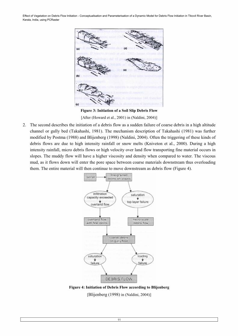
2. The second describes the initiation of a debris flow as a sudden failure of coarse debris in a high altitude channel or gully bed (Takahashi, 1981). The mechanism description of Takahashi (1981) was further modified by Postma (1988) and Blijenberg (1998) (Naldini, 2004). Often the triggering of these kinds of debris flows are due to high intensity rainfall or snow melts (Kniveton et al., 2000). During a high intensity rainfall, micro debris flows or high velocity over land flow transporting fine material occurs in slopes. The muddy flow will have a higher viscosity and density when compared to water. The viscous mud, as it flows down will enter the pore space between coarse materials downstream thus overloading them. The entire material will then continue to move downstream as debris flow (Figure 4).
Figure 4: Initiation of Debris Flow according to Blijenberg
[Blijenberg (1998) in (Naldini, 2004)]

Effect of Vegetation on Debris Flow Initiation - Conceptualisation and Parameterisation of a Dynamic Model for Debris Flow Initiation in Tikovil River Basin, Kerala, India, using PCRaster
12
2.7. Effect of Vegetation
The relationship between forest cover and denudational processes was well understood by early scholars. Pliny, the Elder 1 wrote in his famous book 'The Nat u r a l Hi s t or y' (written in the 1st century) ì Often, disastrous torrents are formed after the felling of mountain woods, which used to hold back clouds and feed on themî (AndrÈassian, 2004). Vegetation effect on slope stability may be broadly classified as either hydrological or mechanical in nature. The mechanical factors arise from the physical interactions of either the foliage or root system of the plant with the slope. The hydrological mechanisms are those intricacies of the hydrological cycle that exist when vegetation is present (Greenway, 1987).
2.7.1. Hydrological Effects
According to van Beek (2002), landuse has a strong influence on soil moisture availability and by that on the activity of rainfall-induced landslides. The effects of vegetation cover on the hydrological processes of shallow landsliding can be subdivided into the loss of precipitation by interception and the removal of soil moisture by evapotranspiration (Figure 5a) (van Beek, 2002). Three main components of canopy interception can be identified. These are the interception loss, water retained by the crown surfaces and later evaporated; throughfall, water falling through and from the leaves to the ground surface; and stemflow, water that trickles along twigs and branches and finally down to the ground surface via the main tree trunks. Interception loss is a primary water loss as it represents water that never enters the soil. The amount depends on the ability of the forest to collect and retain rainfall (interception capacity), storm size and intensity, and evaporation rate. The density, type, and height of the canopy will affect the interception capacity (Oyebande, 1988). Researchersí report that 13% to 23% of gross rainfall is lost by interception in tropical forests. Throughfall and stemflow accounts for the rest of the amount. (Deguchi et al., 2005; Holscher et al., 2004). The interception loss tends to show a negative relation to higher rainfall intensities in tropical rain forests, as observed in Tanzania. When the event was only 1 mm, 70% was intercepted, while only 13.3% was intercepted when the rain event measured 40 mm (Jackson, 1971).
Glade (2003) establishes clear relationships between deforestation and increase in sediment yield by observing evidences on sedimentation over a historic time span. Change in rate of infiltration is another noteworthy hydrological effect of vegetation. When rainwater reaches the ground underneath vegetation, it may stand a better chance of infiltrating than on unvegetated soil (Styczen and Morgan, 1995).
The most significant effect of vegetation on debris flow initiation is the combined process of the removal of moisture from the soil by evaporation and transpiration from the vegetation cover. If defined as two separate events, evaporation is the process whereby liquid water is converted to water vapour (vaporization) and removed from the evaporating surface (vapour removal) i.e., soil and transpiration consists of the vaporization of liquid water contained in plant tissues and the vapour removal to the atmosphere. The process plays a major role in reducing the net water retained in the soil column contributing to the pore pressure especially when the water is contributed through distributed rainfall events and over days. The contribution from this process may be of little significance in cases where high intensity rainfall spanning few minutes or hours results in increased pore pressures. Nevertheless, through modification of the soil moisture content, vegetation affects the frequency at which the soil becomes saturated, which, in turn controls the likelihood of runoff generation or mass soil failure (Styczen and Morgan, 1995).
1 Pliny the Elder or Caius Plinius Secundus (23-79): Roman officer and encyclopedist

Effect of Vegetation on Debris Flow Initiation - Conceptualisation and Parameterisation of a Dynamic Model for Debris Flow Initiation in Tikovil River Basin, Kerala, India, using PCRaster
13
2.7.2. Mechanical Effects
Mechanical effects of vegetation are reinforcement of soil by roots, surcharge, wind-loading and surface protection. The stabilizing reinforcement of roots in soil is supported by landslide inventories that note an increase in landslide frequency following vegetation removal (Schmidt et al., 2001). Roots and rhizomes of the vegetation interact with the soil to produce a composite material in which the roots are fibres of relatively high tensile strength and adhesion embedded in a matrix of lower tensile strength, thereby increasing the effective cohesion of the whole material (Figure 5b). Root induced cohesion is significant in slope stability if only the root density is high at the top 60 cm of soil and is supported by strong tap roots. A schematic diagram of various root types and their contribution in slope stability is provided in (Styczen and Morgan, 1995). Theoretically, tree roots reinforce the soil, increasing soil shear strength, if the roots penetrate through the shear zone (Ocakoglu et al., 2002). Surcharge arises from the additional weight of the vegetation cover on the soil. Surcharge increases the downslope forces on a slope, lowering the resistance of the soil mass to sliding, but also increases the frictional resistance of the soil. It is significant only for trees, as the weight of most herbs and shrubs is too small (Styczen and Morgan, 1995). Wind loading on the vegetation can cause the roots to be pulled out unlike broken apart, reduce soil cohesion and increase the shear stress, if wind direction is along the slope. The process is identified significant only for trees and when the wind velocity exceeds 11 m/s. Vegetation protects the soil mechanically by absorbing directly the impact of walkers, livestock and vehicles (Styczen and Morgan, 1995).
Lancaster and Grant (1999) identify and list three other effects of forest on landslides mechanics as: 1. Effect of stand age on landslides - A nonlinear relationship exists between vegetation age in a regi on
and landslide susceptibility. 2. Wood component of debris flow increases resistance and standing trees resist uprooting - The process is
more related to run out. If the amount of wood material is more in the initiation region and the flow path, the friction for free flow increases and thus run out distance will be less. Same is the case when well established trees are found in the path of a flow.
3. Wood entrainment reduces debris flow mo me n t u m - The mo me n t u m gathered by the flow in a mountainous terrain will be significantly reduced if there are significant amounts of wood material entrained in the flow.
Vegetation in general and root effect in particular needs further research especially in terms of quantifying the same for a dynamic modelling in data deficient conditions. Relationships between stand age and landslide activity needs attention to establish the effects indubitably. Possibility is that as the tree grows older the maximum rooting and thus the maximum root induced cohesion possible will be reached after a certain time. Beyond this time, the stand will keep increasing in biomass and thus the weight that it will exert on the slope will increase and may also attain the stage where it will act as overloading on the slope, thus resulting in slope instability, provided other conditions are sufficed. The loading works in two directions: 1) it increases friction of the soil and hence stability 2) it increases down slope weight and hence decrease the stability; net effect being called surcharge. Importance of such a study is so much so that it is stated in St at e of Worldí s For e st s Report ( F AO, 2003) 'Mountainous forested wa t e r sheds require special attention as they are among the most important fresh water yielding areas in the world but are also source areas for landslides, torrents and floods'.

Effect of Vegetation on Debris Flow Initiation - Conceptualisation and Parameterisation of a Dynamic Model for Debris Flow Initiation in Tikovil River Basin, Kerala, India, using PCRaster
14
Figure 5: Hydrological (a) and Mechanical (b) effects of Vegetation on Slope Stability
[Coppin and Richards (1990) adopted from (van Beek, 2005)]
2.8. Debris Flow Modelling
Brunsden (1999) describes various modelling approaches that are widely used by geomorphologists in the application of landslide studies. He lists them under various subtitles such as Slope Stability Models, Rheological Models and Hydrological Landslide Models. They are not mutually exclusive but are complimentary; one is an input to the other, especially in a dynamic environment.
Slope stability models can mainly be of two types; static models and dynamic process models. Static models consider landslides in their stable state and seek to determine which stimuli cause them to become destabilised (Bromhead, 1996). Dynamic models are models capable to run forward in time, using rules of cause and effect to simulate temporal changes in the landscape (Karssenberg, 2002). Both static and dynamic models are mathematical models.
Dynamic Model can be spatial or non-spatial. A spatial model addresses the spatial and temporal variation of a phenomenon such as debris flow initiation, while a non-spatial model may be the temporal simulation of a cancer cell growth in an organ. Dynamic models can also be classified as deterministic and stochastic models (Karssenberg, 2002). Deterministic models have state variables which have a single value for each location in space and moment in time. Stochastic models are those that deal with chances; if non-spatial, the state variables in the model will be random variables having a certain probability distribution and if spatial, will be random fields. A dynamic model becomes a stochastic model when inputs are stochastic.
Researchers have approached debris flow initiation modelling in several ways. Aleotti (2004) uses a ëthreshold based warning system for debris flow predictioní. The method results in identifying rainfall events, which are potentially capable of initiating debris flows. Glade et al., (2000) uses an ëAntecedent Daily Rainfall Modelí to calculate the regional landslide-triggering rainfall thresholds In this model, first

Effect of Vegetation on Debris Flow Initiation - Conceptualisation and Parameterisation of a Dynamic Model for Debris Flow Initiation in Tikovil River Basin, Kerala, India, using PCRaster
15
introduced by, triggering rainfall conditions are represented by a combination of rainfall occurring in a period before the event (antecedent rainfall) and rainfall on the day of the event. Cellular Automata, a powerful mathematical tool to simulate natural systems, ëSimulation through Computational Innovative methods for the Detection of Debris flow path using Interactive Cellular Automataí is method developed and validated for debris flow studies by University of Calabria, Italy (DíAmbrosio et al., 2003). The model is highly data intensive and that too in a very fine resolution. SCIDICCA S3-hex the latest version of the model provides both numerical outputs as well as map outputs. Precise volumetric assessment of the debris flows can be made; at the same time, hazard zone maps of the region can also be prepared.
Pack et al., (1998) uses a coupled model approach towards addressing slope instability. They use a model named SINMAP, a short form for Stability INdex MAPping and TOPMODEL. They state; ëa promising approach to modelling the spatial distribution of shallow debris slides combines a mechanistic infinite slope stability model with a steady state hydrology model. A steady state hydrology model attempts to assess scenarios assuming a constant water level and thus a constant pore pressure condition, while a dynamic hydrology model simulates the changes in slope stability to changing water levels (and thus pore pressure conditions), based on the rainfall received. Pack et al., (1998) observe that the SINMAP approach applies well to shallow landslides controlled by the convergence of shallow ground water flows, but do not apply to deep-seated instability including deep earthflows and rotational slumps. FLO-2D model built by FLO-2D Software Inc., is a commercially available software capable of simulating debris flow and mud flows. Hyperconcentrated sediment flow is simulated by the FLO-2D model using a quadratic rheological model that includes viscous stress, yield stress, turbulence and dispersive stress terms as a function of sediment concentration (FLO-2D, 2005).
Van Beek (2002) utilizes a similar approach by combining two models, PROBSTAB a limiting equilibrium model based on Mohr-Coulomb failure criterion by which the probability of failure is assessed, is coupled with STARWARS, an acronym for Storage and Redistribution of Water on Agricultural and Revegetated Slopes. He utilizes PC Raster, a dynamic GIS software package distributed for free by Utrecht University. See Chapter 4, Section 4.1 for a detailed description of this model.
2.8.1. Scale Consideration
The scale of application is very important, and also defines if a dynamic modelling approach is feasible or not. One has to decide the representative elementary area (REA) for simulating any natural process, because it influences the structure and the characteristic of the database and the reliability and the precision of the analysis (van Westen et al., 2000). Sensitivity of the model will vary over the areal extent being considered. If to simulate and arrive at meaningful results for a small area, the necessary accuracy of measurements and observations required are too fine to achieve in a limited time. If modelled for a very large area the variability of factors will be too large to justifiably account for, let alone other issues such as computing time and data availability.
2.8.2. Choice of the model
By itself physically based geomorphic models are powerful to assess the influence of specific parameters to the phenomenon being modelling. However they cannot in general give precise predictions. Because geomorphic landscape models are based on quantitative representations of processes, these models are, at least in part, quantitatively testable (Lancaster and Grant, 2003). The deterministic nature of the model makes it suitable to assess scenarios; the uncertainty involved looming upon the predictions, an inevitable compromise to be made.

Effect of Vegetation on Debris Flow Initiation - Conceptualisation and Parameterisation of a Dynamic Model for Debris Flow Initiation in Tikovil River Basin, Kerala, India, using PCRaster
16
Crosta and Frattini (2003) compare several distributed models that simulate debris flow events and conclude that the ideal method for modelling debris flow is through physically based mathematical models, because they explicitly incorporate the dynamic variables that are crucial in the mobilization and motion of debris flows. They conclude that the ideal means of modelling a debris flow is by coupling the infinite slope stability model with the hydrological models able to modulate water table heights in steady or quasi-steady conditions with groundwater flows parallel to the slope. At the basin level, distributed, physically based deterministic modelling represents a major method for considering the spatial variability of controlling parameters (Borga et al., 1998).
Owing to aforesaid reasons supporting the capabilities, it was decided to utilize a deterministic dynamic model for the study. The relative flexibility and adaptability of Van Beekís model made it the most ideal choice. So also was the fact that the model was scripted in an environment modelling language (PCRaster) that had an easy learning curve, but with ample controls to script necessary adaptations. In a developing country as India, it is also necessary to reduce the overall cost of any complex modelling studies. The model, as was implemented using PCRaster, a software distributed for free by Utrecht University also sufficed this consideration.
2.9. The PCRaster Software
The software is a package of powerful set of command lines directly applicable in environmental studies. It is a Geographical Information System, which consists of a set of computer tools for storing, manipulating, analysing and retrieving geographic information, in which data type information is added to all spatial data (Karssenberg, 2002). The core module of the system is a set of PCRaster operations where the operations for Cartographic Modelling are integrated at a high level with the GIS functions of the package. The cartographic modelling core contains functions that are far more powerful than those simple Map Algebra operations. These include functions for visibility analysis, catchment analysis and routing of transport (drainage) of material in a catchment using interactively generated local drain direction maps and transport operations.
These operations together form an algebraic computer language designed for spatial and temporal analysis. A general command in PCRaster will be as follows:
'pcrcalc Resul t = PCRasterOperator(PCRaster Expression/Map)' where, pcrcalc will activate PCRaster operation shell, PCRasterOperator is one of the PCRaster
operations embedded in the software and PCRaster Expression/Map implies that the operator can be applied on either a PCRaster Expression or a Map itself.
For example, in order to derive the minimum slope values from a DEM: 'pcrcalc mi nslope = mapminimum(slope(elevation))'
where, minslope is the resultant map file name, mapminimum is a PCRaster Operator and as well is the slope. The command implies to identify the minimum slope cells with in the slope map derived from the elevation map. This command itself can be nested with other commands and thus a chain of equations can be linked to a single cell to compute a cell state. This process of computing cell states using equations limited in terms of time is called Static Cartographic Modelling. The operations performed represent one static change in the property of cells.
PCRaster contains a Dynamic Modelling Module as well. Herein, the software elaborates spatial modelling a step further by adding the concept of time. This module enables the computation of new cell states as a function of attribute changes over time. The module being linked to the Cartographic Modelling module seamlessly enables the coupled use of both static and dynamic models. The module may also be

Effect of Vegetation on Debris Flow Initiation - Conceptualisation and Parameterisation of a Dynamic Model for Debris Flow Initiation in Tikovil River Basin, Kerala, India, using PCRaster
17
called by the name Dynamic Modelling Language (DML) as it additionally incorporates commands that enable iterations over time, while the Cartographic Module enables computation over space.
Dynamic Modelling in PCRaster is achieved through preparing scripts that contains the inputs, outputs, relationships and equations defining them all nested together, one activating the other or one as an input to another. The script written in DML consists of separate sections. Each section contains a functional part of the script. The sections are: 2. Binding Section: Primary Section of the script. The binding section defines different names in the script:
it binds the database file names to the names of a variable in the model. 3. Area Map Section: Defines that areal extent and the resolution within which the model has to run. 4. Time Section: Controls the time dimension of the model. 5. Initial Section: Contains the cell states at the start of the simulation. This section holds both spatial and
non spatial attribute values 6. Dynamic Section: Defines the operations that result in the map/values for every time step for the cells.
The equations that decide the cell states from time step 1 (t1) to time step n (tn) is defined here. The result of computations of cell state at t1 acts as an input to the cell states at t2 and t2 results as inputs to t3 and so on.
The scripts can be asked to report the results at any point in the computation process using the c o mma n d report . The report can be as ma p s or as a time series file depending on the modelling dema nd. See Appendix 4 for a typical PCRaster dynamic model

Effect of Vegetation on Debris Flow Initiation - Conceptualisation and Parameterisation of a Dynamic Model for Debris Flow Initiation in Tikovil River Basin, Kerala, India, using PCRaster
18
3. Study Area Study area was decided after analysing available data in CESS for various debris flow prone areas
of Kerala. The criteria for choosing the area were a) availability of Soil Thickness Map b) availability of Geotechnical Survey results c) availability of landslide occurrence information and d) availability of fine resolution rainfall information.
The area chosen for the study, Tikovil River Basin is famous for the numerous debris flows that occur almost every year during both monsoon seasons. Since the dynamic model which is used in this study is very data demanding, the chosen study area is also ideal in this regard owing to the data availability from a research project conducted by the Center for Earth Science Studies (CESS) for a 750 km2 region that falls within Idukki and Kottayam districts of Kerala, which encompasses Tikovil River basin as well (Figure 6).
Figure 6: Location Map
3.1. Kerala
Before detailing the characteristics of the study area, which is physiographically part of the Western Ghats mountain system, it is relevant to briefly explain the geomorphic setting of this major orographic feature of Southern India. It is also relevant to explain in few words, the historical significance of the state as a region of continued human interaction with the environment since time immemorial.
Kerala has a land area of 38,863 km2 extending between 8° 17' 30" N and 12° 27' 40" N and 74° 51' 57" E and 77° 24' 47" E (Figure 6). The state is naturally bordered by Ar a b i a n Sea to the we s t and the towering Western Ghats to the east, between which the maximum extent is just about 124 km. From North
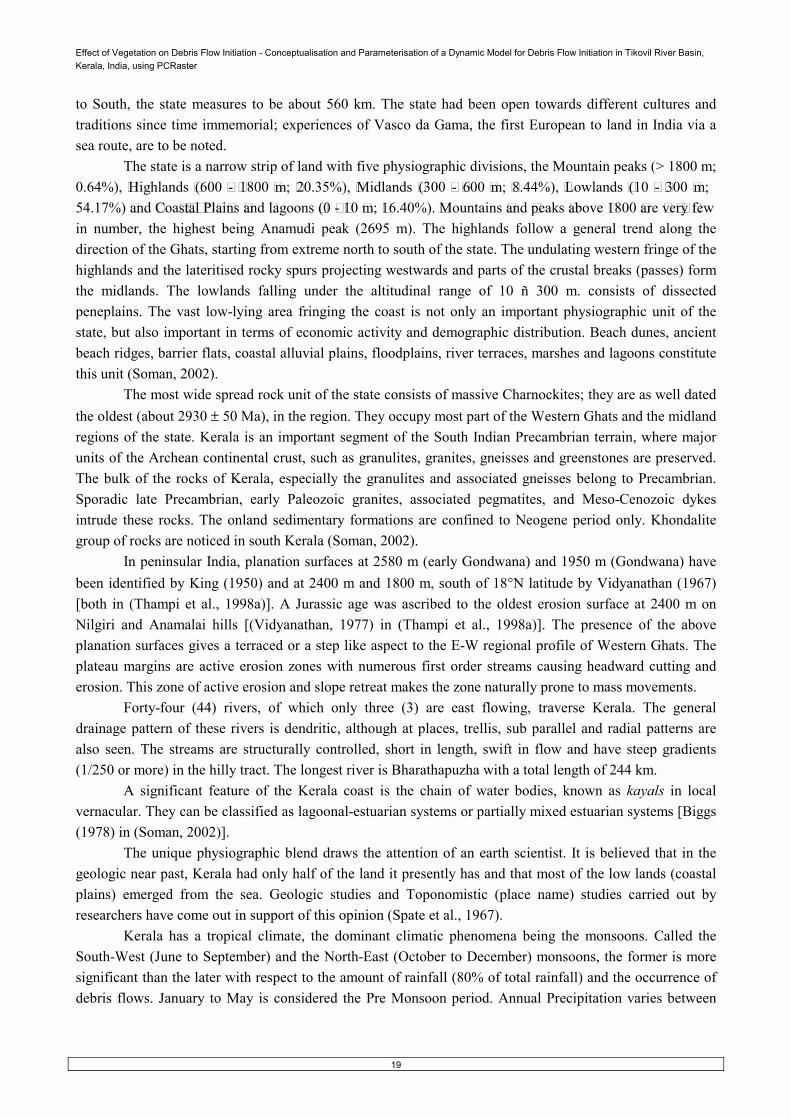
Effect of Vegetation on Debris Flow Initiation - Conceptualisation and Parameterisation of a Dynamic Model for Debris Flow Initiation in Tikovil River Basin, Kerala, India, using PCRaster
19
to South, the state measures to be about 560 km. The state had been open towards different cultures and traditions since time immemorial; experiences of Vasco da Gama, the first European to land in India via a sea route, are to be noted.
The state is a narrow strip of land with five physiographic divisions, the Mountain peaks (> 1800 m; 0.64%), Highlands (600 - 1800 m; 20.35%), Midlands (300 - 600 m; 8.44%), Lowlands (10 - 300 m; 54.17%) and Coa s t a l Pl ai ns and lagoons (0 - 10 m; 16.40%). Mountains and peaks above 1800 are ve r y few in number, the highest being Anamudi peak (2695 m). The highlands follow a general trend along the direction of the Ghats, starting from extreme north to south of the state. The undulating western fringe of the highlands and the lateritised rocky spurs projecting westwards and parts of the crustal breaks (passes) form the midlands. The lowlands falling under the altitudinal range of 10 ñ 300 m. consists of dissected peneplains. The vast low-lying area fringing the coast is not only an important physiographic unit of the state, but also important in terms of economic activity and demographic distribution. Beach dunes, ancient beach ridges, barrier flats, coastal alluvial plains, floodplains, river terraces, marshes and lagoons constitute this unit (Soman, 2002).
The most wide spread rock unit of the state consists of massive Charnockites; they are as well dated the oldest (about 2930 ± 50 Ma), in the region. They occupy most part of the Western Ghats and the midland regions of the state. Kerala is an important segment of the South Indian Precambrian terrain, where major units of the Archean continental crust, such as granulites, granites, gneisses and greenstones are preserved. The bulk of the rocks of Kerala, especially the granulites and associated gneisses belong to Precambrian. Sporadic late Precambrian, early Paleozoic granites, associated pegmatites, and Meso-Cenozoic dykes intrude these rocks. The onland sedimentary formations are confined to Neogene period only. Khondalite group of rocks are noticed in south Kerala (Soman, 2002).
In peninsular India, planation surfaces at 2580 m (early Gondwana) and 1950 m (Gondwana) have been identified by King (1950) and at 2400 m and 1800 m, south of 18°N latitude by Vidyanathan (1967) [both in (Thampi et al., 1998a)]. A Jurassic age was ascribed to the oldest erosion surface at 2400 m on Nilgiri and Anamalai hills [(Vidyanathan, 1977) in (Thampi et al., 1998a)]. The presence of the above planation surfaces gives a terraced or a step like aspect to the E-W regional profile of Western Ghats. The plateau margins are active erosion zones with numerous first order streams causing headward cutting and erosion. This zone of active erosion and slope retreat makes the zone naturally prone to mass movements.
Forty-four (44) rivers, of which only three (3) are east flowing, traverse Kerala. The general drainage pattern of these rivers is dendritic, although at places, trellis, sub parallel and radial patterns are also seen. The streams are structurally controlled, short in length, swift in flow and have steep gradients (1/250 or more) in the hilly tract. The longest river is Bharathapuzha with a total length of 244 km.
A significant feature of the Kerala coast is the chain of water bodies, known as kayals in local vernacular. They can be classified as lagoonal-estuarian systems or partially mixed estuarian systems [Biggs (1978) in (Soman, 2002)].
The unique physiographic blend draws the attention of an earth scientist. It is believed that in the geologic near past, Kerala had only half of the land it presently has and that most of the low lands (coastal plains) emerged from the sea. Geologic studies and Toponomistic (place name) studies carried out by researchers have come out in support of this opinion (Spate et al., 1967).
Kerala has a tropical climate, the dominant climatic phenomena being the monsoons. Called the South-West (June to September) and the North-East (October to December) monsoons, the former is more significant than the later with respect to the amount of rainfall (80% of total rainfall) and the occurrence of debris flows. January to May is considered the Pre Monsoon period. Annual Precipitation varies between

Effect of Vegetation on Debris Flow Initiation - Conceptualisation and Parameterisation of a Dynamic Model for Debris Flow Initiation in Tikovil River Basin, Kerala, India, using PCRaster
20
100 cm (around Chinnar) to 500 cm (around Neriyamangalam), with a state average of about 300 cm (GoK, 2004). The Western Ghats plays a major role in the climatic conditions that prevail all along the state. Wherever there is a breach in the continuity of the mountain system (eg. Palaghat gap), the influence of dry conditions that prevail in the neighbouring state (Tamil Nadu to the east) is felt; the altitudes that the mountain system achieve at various locations also determines the amount of rainfall received. March to May is the hottest with maximum temperatures reaching more than 32°C and the minimums are attained during December to January. Winds over the state are seasonal; diurnal variation is felt owing to the maritime influence. Wind speeds attains 40 - 50 km/hour during and before the monsoon rains (Pisharody, 1992). Annual relative humidity va r i e s between 79 - 80% in the mo r n i n g and 73 - 77% in the evenings.
The soils of Kerala are broadly grouped in ten classes based on the morphological features and physico-chemical properties; they being a) Red Loams, b) lateritic soils, c) coastal alluvial soil, d) riverine alluvial soil, e) greyish Onattukara soil, f) brown hydromorphic soil, g) hydromorphic saline soil, h) acid saline soil, i) black soil and j) forest loam. Lateritic soils are the predominant ones, followed by forest loams and brown hydromorphic soils (SSB (KSDA), 1978).
Kerala state is influenced by several natural hazards such as landslides, coastal erosion, lightning, floods and occasional earthquake activities. The state is classified as moderately active and falls in Zone III of the Seismic Zonation Map of India (IMD, 2002). Recently (2001), the state experienced widespread unusual geological incidents such as well collapse, rapid fluctuations in open well water levels, wavy formations, sprouting up of water in open wells, cracks in buildings, shaking of trees and bushes etc. They are inferred to be because of rapid ground vibrations possibly due to crushing of fault surfaces during movement of crustal blocks (Singh and Mathai, 2004). Though the incidents make an earth scientist suspect neo tectonic activities, the data is insufficient to conclude so as micro level ground deformation studies are yet to take place in the region.
3.2. The Tikovil River Basin
The study area chosen for conducting the modelling is a 55.86 km2 watershed that falls in the central eastern part of the state. It is the upper catchment of Tikovil River that is a west-flowing tributary of Meenachil River. Administratively, the region falls in two districts of Kerala, namely Kottayam and Idukki. The reputation of the region for debris flows is so much that even laymen will enquire whether one has visited Adukkam and Meladukkam (Figure 6) region of Kottayam, if he/she is studying debris flows. For coordinate information see Figure 12.
3.2.1. Physiography
The modelling basin is defined with the outlet as the confluence of Tikovil Ar• and Chatta Puzha. All the physiographic components of a typical debris flow vulnerable zone of Western Ghats are discernible in the region. The eastern part is occupied by the Peerimed plateau, which has all characteristics of a natural peniplanatation surface. Thampi et al., (1998) indicates that plateau margins of highland Kerala have all prerequisites of an active erosion zone where the natural terrain setup is conducive to slope failure/mass movements. The plateau runs northwestñsoutheast creating an escarpment all along the eastern and northeastern part of the area. Surrounding the region as intermittent jut outs from the regular profile of a plateau top are mountain peaks, namely Kurissu Mala♦ South (1195 m), Kolahalamed (1156 m), Kurissu Mala North (1051 m), Illikal Kallu (1042 m) and Mar Mala (1011) (Figure 7). Down-slope the escarpment,
• Ar - Malayalam wo r d fo r stream; Puzha - Malayalam wo r d fo r river ♦ Mala - M a la ya la m for Hi ll

Effect of Vegetation on Debris Flow Initiation - Conceptualisation and Parameterisation of a Dynamic Model for Debris Flow Initiation in Tikovil River Basin, Kerala, India, using PCRaster
21
it is the active youthful upper catchment of Tikovil River that in-turn is a tributary of Minachil River. Considering the broad classification of the physiography of Kerala, the study area has highlands, comprising within it the plateau region, its steep plateau edges, midlands and lowlands, with elevation ranging from 1195 meters at Kurrisu Mala South to 60 meters at the outlet of the defined study area.
3.2.2. Drainage
The study area is drained by 174.95 kms of streams, with the maximum stream order (Strahlerís Method) reached as 5th, the Tikovil Ar (Figure 8). The drainage density is 3.13 km-1 and the channel frequency is 4.98. Majority of the stream segments are 1st order and are perennial, though minor ones may dry out succeeding a less active monsoon. Originating from the Plateau top, the Kala Ar and its tributary Vazhikadavu Ar drains majority of the area. Kala Ar has a 15-meter waterfall while descending from the plateau to the foothills indicating the rejuvenation phase; supporting the fact is that the waterfall is along the plateau margin. Originating from Pulikkal Estate in the north is Aruvikkal Ar, which confluences with Kala Ar downslope to the northwest of Mangalam Mala♦, thereafter called Tikovil Ar. Another major waterfall named Aruvikkal fall is on the southern slope of Mangalam Mala, and has a fall height of 18 meters. The occurrence of these two falls right on the northern and southern flanks of Mangalam Mala leads to infer that the plateau margin runs through these locations. Southern part of the area is drained by a relatively smaller stream, though perennial, named Chatta Puzha. Table 3 details the total drainage length of streams of various orders, bifurcation and length ratios between them. The relatively small bifurcation ratios indicate a quick discharge of the received water and thus provide an indirect inference of the terrain gradient.
Table 3: Drainage Characteristics of the Study Area
Stream Order Number of Segments
Total Drainage Length (km)
Bifurcation Ratio Length Ratio
1 214 105.3 2 50 35.42 4.28 : 1 2.97 : 1 3 10 21.51 5 : 1 1.65 : 1 4 3 7.45 3.33 : 1 2.89 : 1 5 1 5.28 3 : 1 1.41 : 1
♦ Mala ñ Malayalam for Hill

Effect of V
egetation on Debris Flow
Initiation - Conceptualisation and P
arameterisation of a D
ynamic M
odel for Debris Flow
Initiation in Tikovil River B
asin, Kerala, India, using P
CRaster
22
Figure 7: Digital Terrain M
odel
Plateau Margins
Plateau
Debris Flow
s

Effect of Vegetation on Debris Flow Initiation - Conceptualisation and Parameterisation of a Dynamic Model for Debris Flow Initiation in Tikovil River Basin, Kerala, India, using PCRaster
23
3.2.3. Geology
The region has very little variation in geology. Precambrian Crystallines belonging to the charnokite group of rocks predominate. Among the charnockites the major portion is covered by the geneissic variety. Indicting a late Mesozoic tertiary igneous activity is a set of Dolerite d yke s mostly tending northwest - southeast. A small portion of the area towards the south has granites (Figure 8). The general foliation trends N35 W to N45 W, whi c h s o me t i me s swerves to northwest - southeast with high easterly dips of > 50° . The joint pattern indicates a preponderance of j oints running in north-northwest - south-southeast and northwest ñ southeast in the plateau edge and dissected hill region (Thampi et al., 1998a).
3.2.4. Soil
Four major soil associations cover majority of the study area, they being:
Table 4: Major Soil Types in the Study Area
Code No. Map Code Soil Series (Local Names) Classification 62. 4 Agl-Vpm-Ktd (Angel Valley-
Vijayapuram- Koruthode) Clayey-skeletal Ustic Palehumult (Agl), Clayey, Ustic Kandihumult (Vpm) and Clayey-skeletal Ustic Kanhaplohumult (Ktd)
63. 3 Tpl-Tbm (Tulappalli-Thombikandom)
Clayey-skeletal Ustic Haplohumult (Tpl) and Loamy-skeletal Ustic Humitropept (Tbm)
104. 1 Agl-Krd-Ckz (Angel Valley- Kairadi- Chellikuzhi)
Clayey-skeletal Ustic Palehumult (Agl), Clayey Typic Kandiustult (Krd) and Clayey Ustic Kanhaplohumult (Ckz)
133. 2 Kpl-Tpl-Ktd (Kanjirrappally- Tulappalli- Koruthode)
Clayey-skeletal Ustic Kandihaplohumult (Kpl), Clayey-skeletal Ustic Haplohumult (Tpl) and Clayey-skeletal Ustic Kanhaplohumult (Ktd)
K38 5 Kerala 38 Dominant: Clayey, mixed, Ustic Palehumults Associated: Fine, mixed, Ustic Humitropepts and Fine loamy, mixed, Ustic Humitropepts Based on (NBSS, 1999) and (KSLUB, 1995)
Series level data is lacking in the region as detailed surveys are yet to be carried out. The soil codes are those that are originally assigned by NBSS (1999). See Figure 9 for soil type units. Certain unsurveyed portion in the NBSS (1999) Soil Map were filled by extending the existing soil units and also with a soil class from (KSLUB, 1995) for a completely unsurveyed region. Detailed procedure and the reasoning for carrying out such an extrapolation are explained in the section on Data Preparation in Chapter 4.
Geotechnical survey at 12 locations by Thampi et al., (1998) indicates that the region predominantly has sandy soils with an average sand content of 63%. The survey did not reveal much water dispersible clay and is in an order of 3%; silt is 19% and gravel 15%; whereas NBSS maps indicate soils predominantly of clayey type. Provided in Appendix 1 are the geotechnical survey results for the 12 locations. The reason that the NBSS (1999) results and the Geotechnical survey results seems differing in clay content is for the reason that geotechnical surveyors have not dispersed the clay before being tested for its mechanical properties resulting in micro aggregates of clay resembling silt.

Effect of V
egetation on Debris Flow
Initiation - Conceptualisation and P
arameterisation of a D
ynamic M
odel for Debris Flow
Initiation in Tikovil River B
asin, Kerala, India, using P
CRaster
24
Figure 8: Stream Order, Figure 9: Lithology and Figure 10: Soil Types

Effect of Vegetation on Debris Flow Initiation - Conceptualisation and Parameterisation of a Dynamic Model for Debris Flow Initiation in Tikovil River Basin, Kerala, India, using PCRaster
25
3.2.5. Climate
Based on rainfall measurements in the study area from 1965 to 1996, Thampi et al., (1998) conclude that the area has the same general seasonal pattern of the state, with two monsoons and a pre monsoon period. An examination of data from Pullikanam station for which rainfall data is available since 1965 to 1995 and compiled by Thampi et al., indicates that the area receives an annual average rainfall of + 5000 mm. The fact is supported by observed evidence from Kurissu Mala South station for a period of 3 years from 1994 to 1996. The annual average computed for the period from the observed data is 5426 mm with the seasonal division as follows: • South West Monsoon - 4360 mm • Nor t h East Monsoon - 554 mm • Pr e Monsoon - 511 mm
The variability of South West Monsoon Rainfall as observed from Pullikanam station is only 17% whereas Pre Monsoon and North East Monsoon are 40.9% and 40.60% respectively. Rainfall data for 2000 and 2001 collected by Kurissu Mala Christian Ashram shows and annual average of 3611.85 mm; when it was measured 4641.65 mm in 2001 and measured 2582.70 mm in 2000, which was a drought year in the state. For the same period, March registered the highest average maximum temperature of 34.09°C and the lowest average minimum temperature is for the month of December, 21.34°C. The lowest recorded minimum temperature as per available records for the region is on 13th December 2000, which is 16°C and the highest recorded maximum temperature is 36.5°C on 19th January 2000. The records indicate that year 2000 was relatively warmer to that of 2001, and this agrees to the reported fact that May of 2000 was the hottest of the state since 1961 (Staff Reporter, 2000). Monthly Rainfall and number of rainy days for the study area during 2000 ñ 2001 is provided in Figure 11.
The nearest meteorological station to the study area is Kottayam, owned and operated by Rubber Research Institute (a research institution under ICAR) which is about 30 kms aerially to the west of the study area. The nearest possible measurements of other climatic variables are available from this meteorological station. Indian Meterological Department station Kottayam is further down hill. The region experiences moderate temperature conditions, with very high relative humidity. Table 5 compiles the average values of various available climatic variables for the region.
Table 5: Available Meteorological Parameters for the nearest Met Station
Variable Average (2000 ñ 2001)
Temperature Max (RRI) 31.8°C
Temperature Min (RRI) 23.1°C
Relative Humidity Max (RRI) 92%
Relative Humidity Min (RRI) 66.8%
Wind Speed (RRI) 1.4 km/hr
Actual Sunshine Hours (RRI) 6.1
Open Pan Evaporation (RRI) 3.6 mm
Air Pressure (IMD) 1158.33 mb
Vapour Pressure (IMD) 28.46 mb

Effect of Vegetation on Debris Flow Initiation - Conceptualisation and Parameterisation of a Dynamic Model for Debris Flow Initiation in Tikovil River Basin, Kerala, India, using PCRaster
26
Figure 11: Rainfall and Rainy Days in the Study Area (Station: Kurissu Mala Monastery, Year: 2000 - 2001)
0
200
400
600
800
1000
1200Rainfall in mm
0
5
10
15
20
25
30
35
Rainy Days
Rainfall 2001 Rainfall 2000 Rainy Days 2001 Rainy Days 2000
Rainfall 2001 10.00 34.50 99.00 283.75 282.25 1016.2 1114.5 590.65 458.00 459.25 263.25 30.25
Rainfall 2000 0.00 30.75 40.25 65.00 254.25 207.50 150.00 1103.0 298.50 288.50 80.35 64.60
Rainy Days 2001 3 6 15 22 26 30 27 29 19 26 16 1
Rainy Days 2000 0 8 3 13 17 15 12 30 24 28 11 4
Jan Feb Mar Apr May June July Aug Sep Oct Nov Dec
3.2.6. Landuse
Anthropogenic land disturbances in the region started in the late 1880s when colonial exploiters recognized the regionsí potential for tea plantation. Graveyards of foreigners dating to 1919 are found around the town of Vagamon. A few decades in the past, the region was covered with natural vegetation that is prevalent in the tropical highlands. The large-scale migration of settlers from the plains seeking a better fortune in the hills resulted in the clearance of most the natural cover, replanting it originally with coconuts and other hill crops as middle crops. The influx of rubber as a serious commercial crop saw almost the entire region being planted with rubber excluding the plateau tops and grasslands, both excluded due to unfavourable climatic conditions prevailing in the high altitudes.
The region is renowned for its rubber plantations [Figure 13 (a)]. Scientifically called Hevea Brasiliensis Muell. Arg., Rubber is one of the most important commercial crops in Kerala, occupying an area of 4.75 lakh ha. (Srinivasan et al., 2004). As per the landuse map prepared by Thampi et al., (1998) for the study area, 31.13 km2 is occupied by Rubber Plantations (Figure 12). Rubber has a crop life of 20 to 23 years; thus demanding a fresh planting every 23 years. As plantations reach their optimal lifetime, they are slaughtered for wood, exposing the soil beneath to the fury of rain. This makes the landuse maps of the region unreliable, as no one will know which year which plantation will be due for felling; though the general landuse of the area remains the same as slaughtered areas are replanted with rubber. Thus, the soils of a major portion of the area are disturbed at least every 23 years enabling faster rates of infiltration. Most of the rubber plantations have coconut tress as mid crops. Coconut has a much longer crop life and wide spread fibrous roots, thus helping in retaining topsoil. These plantations now occupy a region, which was originally covered by natural montane forests and grasslands.
Following rubber in area is the lush Grasslands and Rock exposures [Figure 13 (b)] that cover an area of 8.23 km2. Though this area has lush growth of grass, they are not of any commercial or fodder use.

Effect of Vegetation on Debris Flow Initiation - Conceptualisation and Parameterisation of a Dynamic Model for Debris Flow Initiation in Tikovil River Basin, Kerala, India, using PCRaster
27
These are grasslands on less weathered rocks where there is very little or no soil. Significant rock outcrops covering a total area of 3.08 km2 are classified separately in the landuse map. The region is bestowed by good grazing pastures, which are also classified separately as Grasslands in the landuse map, indicating their special nature. They cover about 4.04 km2. Degraded forests [Figure 13 (c)] with no dominant species covers 4.55 km2, indicating the vegetative past of the region. They are small patches of shrubby vegetation with mostly shallow soils. Remnants of hard wood trees are seen in many of these patches indicating to their vibrant past. The plateau top near to the village Vagamon is famous for Tea plantations [Figure 13 (d)] covering an area of 3.29 km2. A small patch of 1.5 km2 is occupied by Mixed Crops, mostly Coconut Palms, Plantains, Pinapple etc.
Figure 12: Landuse (Photographs)
a) Rubber b) Grassland+Rock
c) Degraded Forest e) Tea Plantation

Effect of V
egetation on Debris Flow
Initiation - Conceptualisation and P
arameterisation of a D
ynamic M
odel for Debris Flow
Initiation in Tikovil River B
asin, Kerala, India, using P
CRaster
28
Figure 13: Landuse Map
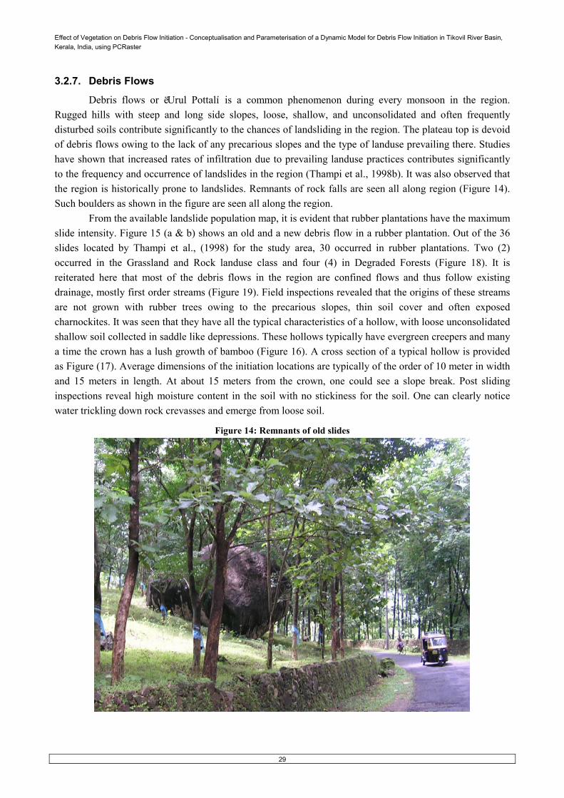
Effect of Vegetation on Debris Flow Initiation - Conceptualisation and Parameterisation of a Dynamic Model for Debris Flow Initiation in Tikovil River Basin, Kerala, India, using PCRaster
29
3.2.7. Debris Flows
Debris flows or ëUrul Pottalí is a common phenomenon during every monsoon in the region. Rugged hills with steep and long side slopes, loose, shallow, and unconsolidated and often frequently disturbed soils contribute significantly to the chances of landsliding in the region. The plateau top is devoid of debris flows owing to the lack of any precarious slopes and the type of landuse prevailing there. Studies have shown that increased rates of infiltration due to prevailing landuse practices contributes significantly to the frequency and occurrence of landslides in the region (Thampi et al., 1998b). It was also observed that the region is historically prone to landslides. Remnants of rock falls are seen all along region (Figure 14). Such boulders as shown in the figure are seen all along the region.
From the available landslide population map, it is evident that rubber plantations have the maximum slide intensity. Figure 15 (a & b) shows an old and a new debris flow in a rubber plantation. Out of the 36 slides located by Thampi et al., (1998) for the study area, 30 occurred in rubber plantations. Two (2) occurred in the Grassland and Rock landuse class and four (4) in Degraded Forests (Figure 18). It is reiterated here that most of the debris flows in the region are confined flows and thus follow existing drainage, mostly first order streams (Figure 19). Field inspections revealed that the origins of these streams are not grown with rubber trees owing to the precarious slopes, thin soil cover and often exposed charnockites. It was seen that they have all the typical characteristics of a hollow, with loose unconsolidated shallow soil collected in saddle like depressions. These hollows typically have evergreen creepers and many a time the crown has a lush growth of bamboo (Figure 16). A cross section of a typical hollow is provided as Figure (17). Average dimensions of the initiation locations are typically of the order of 10 meter in width and 15 meters in length. At about 15 meters from the crown, one could see a slope break. Post sliding inspections reveal high moisture content in the soil with no stickiness for the soil. One can clearly notice water trickling down rock crevasses and emerge from loose soil.
Figure 14: Remnants of old slides

Effect of Vegetation on Debris Flow Initiation - Conceptualisation and Parameterisation of a Dynamic Model for Debris Flow Initiation in Tikovil River Basin, Kerala, India, using PCRaster
30
Figure 15 (a & b): Old (before 2001) and New (2005) Debris Flows in Rubber Plantation
The left over materials at the source have no specific pattern in terms of material dimensions (Figure 17). The flow material is a mixture of sand, silt, wood and weathered rock pieces. The bed rocks at the initiation location and along the run out path are seen to be intact (Figure 14b). No material sorting was seen at the source areas. It was clearly seen that only the overburden was affected by the flows and the bedrock was intact. Enquiries with local inhabitants indicated that often after a flow, the stream that originally used to trickle through narrow channels with very little water will widen and discharge considerable amount of water. Soil thickness at the source points (3 flows, 2005 slides) inspected indicates shallow soils of the order of 0.25 to 0.5 meters. The crown has a soil thickness of 0.2 to 0.3 meters (see illustration in Figure 17). All the located flows in the region have their origin at altitudes higher than 300 meters from MSL. In general, flows are seen to occur in places with slopes greater than 20° and this was confirmed in the field at a recent flow, where the measured average slope is 25°. The sketch of a typical flow is provided in Figure 18. Table 6 details some of the typical characteristics of debris flows in the region as measured during the field work.
Figure 16: The Crown of June 5th 2005 Debris Flow

Effect of Vegetation on Debris Flow Initiation - Conceptualisation and Parameterisation of a Dynamic Model for Debris Flow Initiation in Tikovil River Basin, Kerala, India, using PCRaster
31
The runout length in confined debris flows is difficult to measure; as often they occur through minor order streams that confluence with higher order stream at short distances. The situation prevails in the study area, too. Due to the high discharge, rates and steep gradient the flow material will immediately reach the higher order stream and are washed away leaving no trace of such an incident. This makes it more difficult to measure the exact runout distance and so it is forced to assume that the length of the stream through which the flow occurred is the length of runout. On an average, a first order stream in the region measure about 600 meters in length.
Thus, the area selected has all the reasons to be evaluated in terms of its landslide potential. The landslide hazard zonation map prepared by Thampi et al (1997) explains this well [Figure 20]. Note the dark brown regions of critical areas prone to landslides. The study conducted by Center for Earth Science Studies affirms that the most common type of landslide that occurs in the study area is debris flows, locally known as ëUrul Pottalí. Such mass movements affect only the overburden and leave the underlying crystalline rocks intact (Thampi et al., 1998a).
Figure 17: Cross section of a hollow
Table 6: Characteristics of debris flows in the study area (based on field measurements)
Width of Initiation Location 10 m Length of Initiation Location 15 m Soil thickness along crown margins ≈ 0.3 m Soil thickness at hollows ≈ 0.5 m Run out length from crown 600 m First Prominent slope break at 15 m from crown margin
Bed Rock
Crown Vegetation
Slope Break
Soil Thickness 0.3 m
Accumulation of unconsolidated material

Effect of V
egetation on Debris Flow
Initiation - Conceptualisation and P
arameterisation of a D
ynamic M
odel for Debris Flow
Initiation in Tikovil River B
asin, Kerala, India, using P
CRaster
32
Figure 18 & Figure 19: Landslide Population overlaid on Landuse M
ap and Stream Order M
ap
.
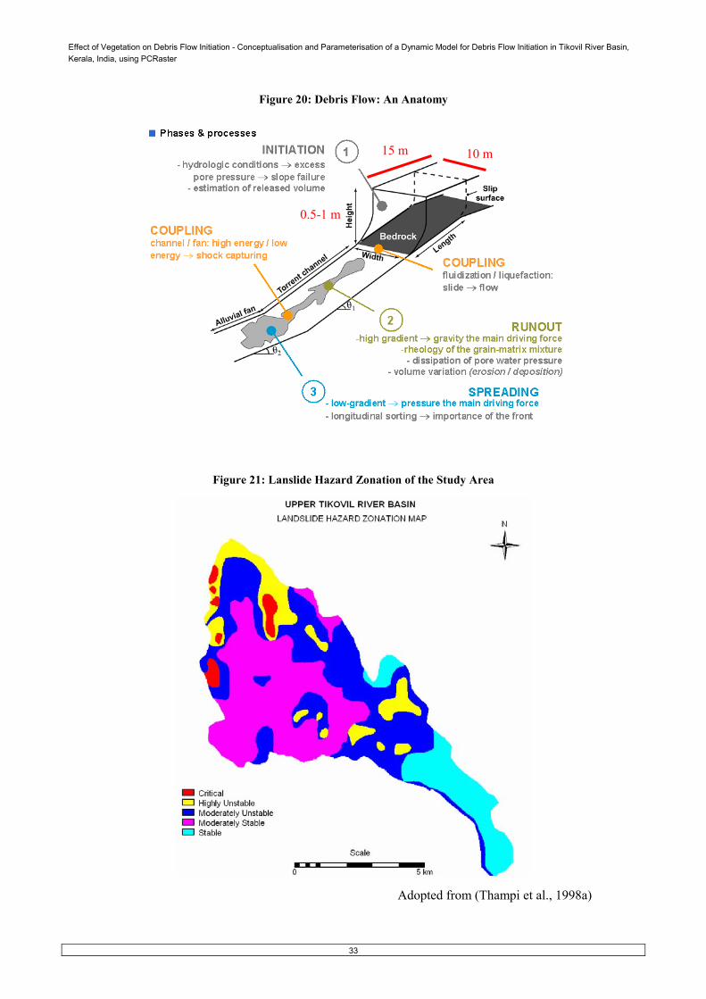
Effect of Vegetation on Debris Flow Initiation - Conceptualisation and Parameterisation of a Dynamic Model for Debris Flow Initiation in Tikovil River Basin, Kerala, India, using PCRaster
33
Figure 20: Debris Flow: An Anatomy
Figure 21: Lanslide Hazard Zonation of the Study Area
Adopted from (Thampi et al., 1998a)
15 m 10 m
0.5-1 m

Effect of Vegetation on Debris Flow Initiation - Conceptualisation and Parameterisation of a Dynamic Model for Debris Flow Initiation in Tikovil River Basin, Kerala, India, using PCRaster
34
4. Materials and Methods
4.1. The Model
The model chosen for conducting the study is physically based and is named as STARWARS + PROBSTAB (van Beek, 2002); also see Chapter 2 Section 2.7. It is a coupled model and is data intensive. The model was chosen, as it allows landuse dependent parameterisation as required for the objectives set out by this research. The model has several additional advantages such as: • Tight coupling of a distributed, physically based hydrological and slope stability model in a GIS
environment (PCRaster); • Dynamic in order to simulate transient hydrological triggers; • Applicable to all cases in which percolation stagnates on a less permeable layer; • Adaptable to various data availability conditions.
In the following paragraphs a brief synthesis of the slope hydrology model (STARWARS) and slope stability model (PROBSTAB) devised by Dr. van Beek is provided. Adaptations made for the present study are explained as well (see Chapter 3 of van Beek (2002) for a more detailed description of the model and the various considerations made by the model designer in achieving a realistic simulation of landslide activity). Only few important assumptions and mathematical equations that are relevant to the present study are clarified here. Also those assumptions and equations that deviate from the original model formulation are explained here.
4.1.1. STARWARS ñ The Slope Hydrology Model
In the coupled model used here, the the slope hydrological model STARWARS is subservient to the stability model and is used to simulate the spatial and temporal occurrence of critical pore pressures; which are the most crucial component controlling slope stability of steep slopes mantled with loose material in humid tropics. In the Kerala region, the formation of perched water tables particularly during the SW monsoon leads to elevated pore pressures and the role of these transient hydrological conditions as potential triggers mu s t be investigated. Landuse dynami cs have a direct influence on the hydrology and mu s t be included if the hazard of rainfall-induced landslides and debris flows are to be quantified and remedial measures evaluated.
STARWARS simulates the spatial and temporal dynamics of moisture content and perched water levels in response to gross rainfall and evapotranspiration. Thus, it models percolation through the unsaturated zone and lateral saturated flow over a semi-pervious bedrock contact. Both the saturated and unsaturated zones are assumed freely draining and the groundwater levels unconfined.
In the model any rainfall is prone to interception by the vegetation canopy. A fraction reaches the soil surface unhampered as bulk throughfall whereas the remainder is intercepted and is only passed on as leaf drip when the maximum canopy storage is exceeded. Meanwhile, the intercepted rainfall can be lost to the potential evapotranspiration, thus freeing storage capacity for the next rainfall event. Any evaporation from the canopy is subtracted from the potential evapotranspiration that is passed to the surface. Ideally, stemflow should also be accounted for but this process is difficult to quantify and most times negligible compared to throughfall and leaf drip. Since no measurements on interception were available for the region, remotely sensed data have been used to fill this gap in the parameterisation of the model.

Effect of Vegetation on Debris Flow Initiation - Conceptualisation and Parameterisation of a Dynamic Model for Debris Flow Initiation in Tikovil River Basin, Kerala, India, using PCRaster
35
After the evaluation of any interception of rainfall by the canopy, rainfall and potential evapotranspiration are passed to the soil. If surface detention is already available, it is liable to evaporation and the remaining potential evapotanspiration that can be lost from the soil is modified accordingly. The net rainfall is added to any remaining surface detention, which can infiltrate. Any surface detention in excess of infiltration or return flow is passed on as surface runoff.
The soil profile is subdivided into three vertical layers to allow for variations in the soil properties with depth and the perched water table can move freely within the soil column, thus reducing the depth of the unsaturated zone. In the model infiltration is added to the upper most unsaturated layer or in the case of full saturation to the saturated zone directly. Percolation through the unsaturated zone proceeds from layer to layer and is driven by gravitational unsaturated flow only. This flow is proportional to the unsaturated hydraulic conductivity, k(θE), which is a function of the effective degree of saturation, θE. To facilitate the calculation of the unsaturated hydraulic conductivity and to check on the available water, all storages are expressed as water slice and the conversion from volumetric moisture content (θ or VMC) to the effective degree of saturation is calculated as follows:
ressat
resE θθ
θθθ−
−=
Relative Degree of Saturation: [1]
where, θ is volumetric moisture content (VMC), θsat the saturated moisture content which is set to Porosity and θres the residual moisture content.
The unsaturated hydraulic conductivity determines the travel time to pass each unsaturated layer and the percolation is directly proportional to the fraction of moisture that could pass the contact within one timestep. Soil water retention is described in terms of the SWRC formulation of Farrel and Larson (1972) and the corresponding unsaturated hydraulic conductivity described by the capillary analogy of Millington and Quirk (1959, 1961). With rising ground water levels, the travel times reduce and to ensure numerical stability the actual flux is calculated using a central finite difference solution including the additional changes in the unsaturated storage that arise from transpiration (lumped with soil evapotranspiration) and infiltration/percolation. After obtaining the maximum transpiration as the product of the remaining potential evapotranspiration and the crop factor (van Beek, 2002), the actual evapotranspiration, therefore, is proportional to the available storage relative to the total storage of the soil profile. The actual evapotranspiration is distributed over the saturated and unsaturated zones according to the available storage. The procedure provides robust estimates of sustainable percolation and evapotranspiration rates in the soil.
Evapotranspiration and percolation lead to a change in the saturated storage that translates into a rise of the water table that depends on the available unsaturated pore space. However, some leakage at the base of the soil column can occur and this can lower the water table or prevent its formation altogether as long as the percolation rate from the unsaturated zone is insufficient. This base loss is simulated by imposing a constant flux into a fourth, infinite layer (i.e., k(θE BC)). If no groundwater is present, this constant flux is the maximum percolation that can be passed to the bedrock, if groundwater is present, the flux increases proportional to the vertical gradient and the saturated hydraulic conductivity of the bedrock layer.
After evaluation of the vertical changes in water height for the current timestep, saturated lateral flow is considered. The elevation of the water table is used as the total head to calculate the gradient of the saturated flow in the X- and Y-directions of the grid using a simple explicit, forward finite difference solution. The resulting lateral flow leads to a new water level and change in the depth of the unsaturated

Effect of Vegetation on Debris Flow Initiation - Conceptualisation and Parameterisation of a Dynamic Model for Debris Flow Initiation in Tikovil River Basin, Kerala, India, using PCRaster
36
zone. The effective degree of saturation of the overlying unsaturated layer is used if water a fully saturated layer cavitates, if the soil becomes fully saturated any water in excess of the available storage exfiltrates as return flow to the surface.
4.1.1.1. Effects of Vegetation
In order to account for the vegetation effects on slope hydrology in the model several parameters were necessary (See Table 7 for a list). Estimates of the crucial parameters such as interception and bulk throughfall were not readily available for the region from any literature sources. This necessitated some of the empirical approaches stated below which are based on satellite remote sensing derived datasets; conducting a detailed field work for acquiring the data for computing these parameters was beyond the scope of the present study.
Interception was calculated using Astonís Equation, linking it to Normalized Difference Vegetation Index (NDVI hereafter) thereby availing the option of utilizing data products available from satellites having finer temporal resolution such as Moderate Resolution Imaging Spectroradiometer (MODIS) onboard Terra (EOS AM) and Aqua (EOS PM) satellites of NASA. Interception is:
−=
−max
*
max exp1** SPk
c
cum
SfS
Astonís Equation for Canopy Interception: [2]
where, S is the interception (in mm), fc is the fractional vegetation cover (-), Smax the maximum canopy storage (mm), -k the correction factor for vegetation density (equals 0.046*LAI) (-), and Pcum the cumulative rainfall (mm). Smax was computed from Leaf Area Index (LAI) using the equation proposed by Von Hoyningen-Huene (1981) as:
2max *00575.0*498.0935.0 LAILAIS −+=
Von Hoyningen-Huene Equation for Maximum Canopy Storage: [3]
LAI was computed from fractional vegetation cover using the equation proposed by Campbell and Norman (1998) as cited by Walthall et al., (2004) and is:
( )cfLAI −−= 1ln2 Leaf Area Index: [4]
where, fc is the fractional vegetation cover (-). Fractional vegetation cover was computed with the equation suggested by Walthall et al., (2004)
and is:
ck
NDVINDVINDVINDVIf i
c
−−=
minmax
max
Fractional Vegetation Cover: [5]
where, kc is the crop coefficient of the respective landuse, NDVImax is the maximum NDVI for the given image, NDVImin is the minimum NDVI for the given image and NDVIi is the NDVI of a particular pixel. It is advised by many researchers (Lele et al., 2005; Walthall et al., 2004) that care has to be taken to avoid the occurrence of outliers in NDVI values due to astray data errors. Though discussion is ongoing

Effect of Vegetation on Debris Flow Initiation - Conceptualisation and Parameterisation of a Dynamic Model for Debris Flow Initiation in Tikovil River Basin, Kerala, India, using PCRaster
37
among researchers on how to avoid spuriousness in the data, a wise method is to visually identify the true vegetation pixels and true soil pixels from the original image bands in a given area and use them as the Maximum and Minimum values of NDVI, as was adopted in this research.
The bulk throughfall coefficient (BT hereafter) was computed as suggested by van Beek (2002) (Eq. 6) and is not used as a fitting parameter for any reasons including model calibration thus making it a valid assumption for all practical purposes of the present research. The coefficient also referred to as free throughfall coefficient accounts for the direct througfall occurring during a rain event.
−=LAI
BT 11
Bulk Throughfall Coefficient: [6]
The interception deducted rainfall, reaches the surface and is stored as surface detention. Both interception and surface detention are subjected to evaporation. The evapotranspiration (Erc, mm.day ñ1) is accounted using Hargreaves equation as against the original Penmanís equation as used in by the model designer; the calculation is carried out outside the model and the values are provided as a time series file. The equation is temperature based and provides reasonable estimates of reference crop evapotranspiration (Erc) (Shuttleworth, 1993). The model corrects the Erc to the actual evapotranspiration using the crop coefficient approach proposed by Allen at al., (1998), thereby accommodating the fact of limited soil water availability and the presence of vegetation.
Based on the above stated theoretical background the model provides temporal volumetric moisture contents and water levels as outputs. The Volumetric Moisture Contents are converted to the respective Effective Degree of Saturation and the predicted Water Levels are input to the slope instability model.
4.1.2. PROBSTAB ñ The Slope Stability Model
The slope stability model is based on the infinite slope form of the Mohr-Coulomb failure law as expressed by the ratio of stabilizing forces (shear strength) to destabilizing forces (shear stress) on a failure plane parallel to the ground surface. The model is modified to account for root-induced cohesion and surcharge that were not originally considered by van Beek (2002). The equation used is:
( ) ( ) [ ]( )[ ] ββγγ
φβγγγcossin
tancos2
vss
vwwss
ZZZCrCsFS
++−++
=
Factor of Safety: [7] where, Cs and Cr are the soil and root induced cohesion respectively (kPa), γs unit weight of soil, γw unit of weight of water, γv surcharge due to weight of vegetation (kPa), Zs soil thickness (m), Zw water height (m), β slope angle and φ angle of internal friction. The unit weight of soil is an addition of γs sat and γs unsat and γv, the unit weight of saturated soil, unsaturated soil and vegetation surcharge, respectively.
For computing the unsaturated unit weight and further incorporate it into a probability of failure assessment using FOSM approach, the relative degree of saturation is converted to the effective degree of saturation by multiplying it with the thickness of the unsaturated zone above the groundwater table. Equation 9 illustrates the way in which this was achieved for the present study assuming the entire soil thickness as a single column and the plane of failure coincides with the plane of contact between soil and bedrock.
( ) ( )( ) ( )321321
333222111 )(HHHZZZHZHZHZ EEE
eff ++−++−+−+−
=θθθθ
Effective Degree of Saturation: [8]

Effect of Vegetation on Debris Flow Initiation - Conceptualisation and Parameterisation of a Dynamic Model for Debris Flow Initiation in Tikovil River Basin, Kerala, India, using PCRaster
38
where, θeff is the effective degr ee of saturation, Z1... 3 thickness of each soil layer (m), θE(1Ö 3) the relative degree of saturation of each soil layer, H1... 3 wa t e r levels of each soil layer (m). By vi r t u e of this computation, the model incorporates the weight of unsaturated soil column (γunsat) in calculating the factor of safety, a factor not commonly addressed in the textbook illustrations of infinite slope stability and is ignored as irrelevant in most cases.
Original PROBSTAB treats the variability of the shear strength rigorously. Since additional vegetation effects are considered here and a less computationally demanding method would be preferred the simpler First Order Second Moment (FOSM) approach has been adopted, in terms that the model provides an average, first negative and first positive standard deviation conditions of the safety factor based on the average and standard deviation inputs of the actual slope stability influencing parameters. The slope hydrology parameters are avoided for computing the FOSM based Probability of Failure. The method was computationally more economic than the original more exhaustive PROBSTAB used by the model designer, given the fact that the results of the FOSM script can also provide an estimation of the model sensitivity to the defined set of slope stability parameters excluding the slope hydrology parameters. It is assumed that all uncertainty arises from natural variability and sampling errors. The mathematics involved in the computation of Probability of Failure using FOSM is given below.
FOSM assumes that the performance of a variable Y, such as ëFactor of Safetyí is a function G of random input variables X1, X2, X3 . . .Xn:
),...,,( 321 nXXXXGFS = Variable Performance: [9]
),...,,()( 321 nXXXXGFSM = Mean Factor of Safety: [10]
where, M(FS) is the factor of safety computed with the mean values of all the input variables and function G is the infinite slope model.
Cumulative Variance of FS based on each parameter is obtained based on the first negative and positive standard deviations.
)(...)()()( 22
22
2
21
22
1n
n
XXFX
XFX
XFFSVar σσσ
∆∆++
∆∆+
∆∆=
222
21
2...
22)(
∆++
∆+
∆= NFFFFSVar
Cumulative Variance of Factor of Safety: [11]
Assuming probability of failure as normally distributed, the Z scores are obtained as:
)()(
FSVarFSMFSZ −=
Z score assuming normal distribution: [12]
where, FS is the value of the factor of safety for which the probability of failure is determined, i.e. FS = 1. This can range between -∞ < F ≤ 1.
In reality, many natural variables and the factor of safety will be censored as the shearing resistance can not be negative (van Beek, 2002). F cannot be smaller or equal to zero. To ensure that there is no negative tail in P(F<=1), one could use the log-transform of F. Since M[F] and V[F] are based on a normal distribution, it is necessary to find them for a log-normal one, where y= ln(F). which have the log-normal

Effect of Vegetation on Debris Flow Initiation - Conceptualisation and Parameterisation of a Dynamic Model for Debris Flow Initiation in Tikovil River Basin, Kerala, India, using PCRaster
39
mean and variance of alpha= M[y]= Ω ln(M[F]4/(M[F]2+V[F])) and beta= V[y]= ln((M[F]2+V[F])/M[F]2). By using the Coefficient of Variation (COV) of M/VΩ the Z-score can be easily calculated as it allows one to express the mean and standard deviation into one another: Zlog= (M[y]-E[y])/(V[y]). Now the expected value of E[y]= E[ln(F=1)]= 0, so by using the COV, the Z = Alpha/Beta, which expands to:
[ ][ ]
[ ]( )22
ln1ln
1ln
FCOV
FCOVFM
Z+
+=
So a log-normal distribution of F is used. In order to obtain the Log-transformation of F the following formulae are used:
Standard deviation of the factor of safety after varying every parameter is obtained as:
)()( FSVarFSSD = Standard Deviation of Factor of Safety: [13]
Coefficient of variation is obtained based on the standard deviation as:
)()()(
FSMFSSDFSCoeffVar =
Coefficient of Variation of Factor of Safety: [14]
The coefficient of variation is obtained as it is easy to arrive at the logarithmic term of FS using the coefficient of variation.
Logarithmic Term of FS is:
( ) 2)(1ln FSCoeffVarFS += Logarithmic term of Factor of Safety: [15]
Z Score of Factor of Safety assuming as having log normal distribution is:
( )( )( )FS
FSFSMZ
lnln)ln(/)((ln
ln =
Z score assuming logarithmic distribution: [16]
The probability of failure is computed from the Z score using a standard normal distribution. In the process the script as well computes changes that the factor of safety has with the change in
each input parameter to the negative and positive standard deviations. These maps are a pragmatic estimate of the sensitivity that the factor of safety has to each of the input parameters in terms of M[F] and V[F]. Though the transient hydrological conditions have a reasonable contribution to the computed factor of safety, it is not considered for the probability of failure calculation and to assess the sensitivity of the model.
A conceptual schema of the coupled model is incorporated below and the model inputs and outputs are explained in Table 7:

Effect of Vegetation on Debris Flow Initiation - Conceptualisation and Parameterisation of a Dynamic Model for Debris Flow Initiation in Tikovil River Basin, Kerala, India, using PCRaster
40
Figure 22: Coupled Model of STARWARS + PROBSTAB
[Based on:- van Beek, 2002]

Effect of Vegetation on Debris Flow Initiation - Conceptualisation and Parameterisation of a Dynamic Model for Debris Flow Initiation in Tikovil River Basin, Kerala, India, using PCRaster
41
Table 7: Model in & output of ASTONís, STARWARS, Effective Degree of Saturation and PROBSTAB Models Note that the dynamic outputs from each model are the input to the subsequent model. The table has to be read column wise starting from inputs to outputs and the sequence is ASTONís, STARWARS, Effective
Degree of Saturation and PROBSTAB.
Model Component
ASTONíS Hydrology ñ STARWARS
Effective Degree of Saturation
Stability - PROBSTAB
Model Input Schematisation DEM (m)
Soil Depth D(z) (m) Global boundary conditions • Matric suction for lower boundary condition hBC (m)
• Matric suction at field capacity, 1st layer hFC (m)
Global ñ Landuse dependent • Crop Factor kc (-)
Constant Parameter values
Monthly Averages • Fractional Vegetation Cover Kfac (-)
• Maximum Canopy Storage Smax (mm)
• Correction Factor k (-)
Soil Type, Landuse and Depth Dependent • Saturated hydraulic conductivity ksat (m.d-1)
• Porosity n (m3.m-3) • Air entry value hA (m)
• SWRC Slope α (-)
Layer Dependent • Saturated Moisture Content θsat
Layer Dependent • Cohesion C (kPa) • Angle of Internal Friction φ (°)
• Dry bulk unit weight of the soil γs (kN.m-3)
• Root induced Cohesion Cr (kPa)
• Bulk unit weight of Vegetation S [kN/m3]
Dynamic Input ñ All
timesteps
• Reference Potential Evapotranspiration Erc (mm.d-1)
• Rainfall RF (mm.d-1)
• Effective Rainfall Eff RF (m.d-1)
• Remnant of Evapotranspiration to occur from Soil Erc Soil (m.d-1)
• Groundwater level WL (m)
• Volumetric Soil Moisture Content VMC (m3.m-3)
• Effective Degree of Saturation (-)
• Groundwater level WL (m)
Initial conditions ñ state variables
• Interception Ic (m) • Effective Rainfall Eff RF (m.d-1)
• Remnant of Evapotranspiration to occur from Soil Erc Soil (m.d-1)
• Groundwater level WL (m)
• Volumetric Soil Moisture Content VMC (m3.m-3)
• Effective Degree of Saturation (-)
• Factor of safety F(-) (Set to 999 indicating that the simulation starts with stable conditions)

Effect of Vegetation on Debris Flow Initiation - Conceptualisation and Parameterisation of a Dynamic Model for Debris Flow Initiation in Tikovil River Basin, Kerala, India, using PCRaster
42
Model Output Maps and Timeseries
• Interception Ic (m) • Effective Rainfall Eff RF (m.d-1)
• Remnant of Evapotranspiration to occur from Soil Erc Soil (m.d-1)
• Groundwater level WL (m)
• Volumetric Soil Moisture Content VMC (m3.m-3)
• Effective Degree of Saturation (-)
• Factor of safety [F(-)]
• Probability of failure [PF (-)]
• Sensitivity Maps
[Based on:- van Beek, 2002]
Root induced cohesion and surcharge was incorporated into the PROBSTAB section of the model, but were calculated outside the model and provided as inputs. The equations used are elaborated in Section 4.5. The infinite slope model considers shear strength as numerator and the shear stress as denominator. Root induced cohesion was added to the numerator of the equation along side normal soil cohesion and the vegetation surcharge was added to both the numerator and the denominator, reason for which is well explained in Chapter 2 Section 6.2.
The challenge involved was in parameterising the model. Due to lack of proper field estimates of the inputs in a data deficient country as India, it was necessary to assume the values through scientific and logical computations. Literature derived values are as well resorted to, whenever it was deemed pertinent.
4.2. The Data
Extensive data sets were required to parameterise the model on a daily time step. This necessitated the collection of data from various sources. Certain parameters for which direct measurements are not available were estimated using established equations. Table 8 compiles various datasets used for parametrising the model with the respective sources. The use of a particular data in the research is also provided corresponding to each data. A brief description of the source institutions is provided in Appendix 2.
Table 8: Data, Sources and Use
Sl No. Data Type Source What for 1. Contour Map (20 m) Vector Layer
(1:50,000) Thampi et al., 1998 (CESS)
DEM Generation, LDD and Slope maps
2. Soil Depth Map (m) Vector Layer (1:50,000)
Thampi et al., 1998 (CESS)
Estimation of Overburden, Soil hydraulic properties etc.
3. Landuse Map Vector Layer (1:50,000)
Thampi et al., 1998 (CESS)
ETo to ETk, Infiltration, Root Induced Cohesion and Surcharge
4. Soil Type Map Vector Layers (1:50,000)
(NBSS&LUP, 1999) and (KSLUB, 1995)
The unit to parameterise Soil Geotechnical Properties, Soil Hydraulic Properties
5. Geotechnical Properties of Soils (Cohesion, Angle of Internal Friction, Bulk
Vector Layer (Points)
Thampi et al., 1998 (CESS)
Calculation of Safety Factor, Soil Hydraulic Properties

Effect of Vegetation on Debris Flow Initiation - Conceptualisation and Parameterisation of a Dynamic Model for Debris Flow Initiation in Tikovil River Basin, Kerala, India, using PCRaster
43
Density and Degree of Saturation)
6. Normalized Difference Vegetation Index (NDVI) - 16 day composites, 2 per month
Raster Layers (MODIS derived 250 meter resolution)
EOS Geo-gateway
LAI, Fractional Vegetation Cover, Interception, Storage
7. Rainfall (mm) Excel Sheet (Seasonal total rainfall for 1965-1995, daily for 2000-2001 and seasonal total for 2004-2005)
Pullikanam Estate, Kurisumala Christian Monastery and The Hindu Newspaper
Effective Rainfall reaching the ground
8. Temperature (°C), [Min & Max]
Excel Sheet (1 location; daily for 2000 and 2001)
Rubber Research Institute of India, Kottayam
Reference Evapotranspiration
9. Root Tensile Strength Primary data (Estimated for 3 sets of 6 samples for rubber trees)
Measured using a Universal Testing Machine
10. Root Shear Primary data (Estimate for 10 points along a 2005 debris flow)
11. Root Count Primary data (1 m * 1m * 1m pit at one location)
Measured in field
Root Induced Cohesion
12. Average weight of a Rubber Tree
Primary data Interview with rubber planters
Surcharge
All the vector layers and the tables were later converted to PCRaster *.map and ASCII format respectively.
4.3. Methods
The research wo r k wa s di vi ded into two part s - Fi r s t , a literature revi ew and fi el dwork phase to suffice the first objective and second, parameterisation of the model to suffice objectives two, three, four and five. Time utilization of the thesis work is provided in Appendix 3.

Effect of Vegetation on Debris Flow Initiation - Conceptualisation and Parameterisation of a Dynamic Model for Debris Flow Initiation in Tikovil River Basin, Kerala, India, using PCRaster
44
4.3.1. Choice of Modelling Resolution
Given the fact that DTM generated from 20 m contour interval is the best available for the area constrains the best possible modelling resolution to 20 m. A 20 m by 20 m pixel will capture all the best of information available in the contour map with 20 m contour interval. Any finer resolution will not improve the model results but any coarser resolution will degrade the precision as it will result in the generalisation of the topographical convergence of subsurface flow and slope stability. It is further justified with the scale of maps (1:50,000) of other available inputs.
4.3.2. Choice of Model Validation Period and Time-step
Once the study area was decided, a detailed literature search was initiated in acquiring as much information as possible for the area. Most crucial data sets such as landuse map, soil thickness map, landslide inventory, digital terrain model, drainage, geotechnical properties of the soils etc. were available from Thampi et al., (1998). Rainfall being the next important input, search for the same led to Kurisumala Christian Monastery and yielded uninterrupted rainfall data for two years, 2000 and 2001 with a daily resolution. Over one hundred and eighty (180) journal articles, books, websites and other media were referred for the research work. The availability of rainfall and the fact that several unexplained geologic phenomena occurred in the region during 2000 ñ 2001 (Singh and John Mathai, 2004) coupled with the occurrence of several debris flows were valid reasons to fix the model validation period.
As nature cannot be fully abstracted, any model needs to have trade off between the modelís capability to simulate the real world adequately on the one side and the uncertainty involved. Constrains of the spatial resolution of available datasets limits the temporal resolution of the model. A decreased spatial resolution reduces the ability of the model to represent the topographical effects on the hydrology on the slope stability adequately [Zang & Montgomery in (van Beek, 2002)]. Initial runs of the slope hydrology model for the study area, with the given spatial resolution indicated numerical instability and thus a quarter day time-step was adopted, however, results were analysed for the daily variation. Though quarter day time-steps were used, the resolution of the rainfall data used was daily. This was converted to quarter days by dividing the rainfall equally. A daily time-step simulation was adopted from the slope stability model.
4.3.3. Data Preparation
4.3.3.1. Field Work
Three field works were carried out. The first was to familiarize with the study area and establish contacts. Second was to verify the available maps such as landuse, soil thickness and debris flow population, and to estimate the parameters for root induced cohesion calculation and groundwater levels. The third fieldwork was to locate those flows that occurred during the period 2000ñ2001 and also to get a firsthand feel of the extreme conditions that result in a debris flow in the study area as the third fieldwork coincided with extreme rain events in the region. Water levels were measured in 11 well locations, spread across the study area.
The first fieldwork was carried out along with the supervisors from IIRS and CESS. The fieldwork confirmed the logic of choice of study area and provided enough inspiration to go further with the research. A debris flow that occurred on June 5th 2005 was inspected and measured for the width of initiation points, landuse, soil moisture conditions, bedrock status, slope, etc. The flow occurred on the southern flank of the study area, just outside the boundary. But other factors being similar with the study area, the location is a true representative of the debris flows that occurs in the region. Few other old debris flow scars were as well examined during the fieldwork.

Effect of Vegetation on Debris Flow Initiation - Conceptualisation and Parameterisation of a Dynamic Model for Debris Flow Initiation in Tikovil River Basin, Kerala, India, using PCRaster
45
Field investigations and preceding research works (Thampi et al., 1995; Thampi et al., 1998b) indicates that the landuse practices prevailing in the region has a significant role in the initiation locations of debris flows. In order to plant rubber, planters often alter the entire terrain; natural streams are obstructed, diverted and confined to plantation grounds enabling a very high rate of infiltration. Adding to the process is the contour bunding practice that prevails in the region. Altered channels are constrained to every bund and during monsoon season, heavy downpour results in water stagnation and saturation of the bunded soil columns resulting in mobilisation of high rates of shear stress (Figure 23 (a)). It was also observed during the fieldwork that water stagnated on the surface from a rain event is retained and not allowed to flow downstream, thus creating highly saturated soil columns (Figure 23 (b)).
A model that deals with the initiation of debris flows in the region needs to consider this process and identify some methods to parameterise the effects of these practices. A possible method to parameterise the practice is by altering the DEM and thereby modifying the model of the terrain, subsequently increasing the percolation rate, and by letting the surface detention from a particular rain event remain on the terrain for a designated number of timesteps that follow. Obviously this will result in highly saturated conditions. But such an approach will detail the actual factors that are really contributing to slope stability.
Figure 23 (a & b): Contour Bunding & Drainage Alteration, and Surface Detention
Figure 24: A typical hollow
Field observations revealed that presence and absence of vegetation has a significant effect on the initiation points. As described in Chapter 3 Section 3.2.7 Paragraph 2 ëthe initiation points of flows inspected were devoid of any vegetation cover thus both hydrological and slope stability contributions from vegetation cover completely absentí. However, the REA of the present modelling exercise constrains the possibility to incorporate this aspect. Moreover, though known flow initiation locations are devoid of

Effect of Vegetation on Debris Flow Initiation - Conceptualisation and Parameterisation of a Dynamic Model for Debris Flow Initiation in Tikovil River Basin, Kerala, India, using PCRaster
46
vegetation cover, the relative significance of vegetation can be evaluated by parameterising the mo. Interestingly most of them had some exposed rock nearer to the crown (Figure 24). Note in the picture that rubber trees surround the hollow. A realistic prediction needs to account for this absence of vegetation contributions to slope stability in hollows. This is possible only by adopting a stochastic approach, by virtue of which a modeller will have to introduce a new parameter possibly in the form of a map that indicates all the hollows present in the region. Every known flow initiation locations are equally relevant as the ones that are possible hollows. Long recurrence intervals and the apparent importance of high intensity rainfall events indicate that a lack of historic debris flows from specific hollows is by no means an indicator of future stability (Melelli and Taramelli, 2004). While modelling the phenomena, these points may thus be parameterised with its true characteristics, avoiding generalization. But this to be feasible the model should be parameterised in a much finer resolution than the present work. Satellite remote sensing and aerial photos have relatively lesser use in this regard especially where colluvial deposits in subtle topographic depressions are hidden by thick canopy. A viable solution is geomorphic mapping, as the margins of colluvial deposits in hollows are generally coincident with a change from convex to concave slope profile (Melelli and Taramelli, 2004).
Another issue to be addressed while designing a model for predictions of debris flow initiation in the area is the cyclical process of rubber plantation slaughtering. Every 20 to 23 years, rubber plants achieve maturity and are of further no use for extraction of latex. Plantations with trees having achieved maturity are subjected to clear felling. Figure 23 (a) shows a recently slaughtered plantation being readied for replanting. This exposes ground to direct rainfall and subsequently results in increased infiltration and runoff. The contributing hydrological effect of vegetation to slope stability is nullified in such areas.
Slow process such as splash erosion may also occur owing to the energy of the raindrops. The effect of this can be addressed through a time-series landuse/landcover maps derived using satellite data having fine temporal resolution. At least the most critical positive effects of vegetation on slope stability such as interception and evapotranspiration are thus to have fine temporal resolution which can be achieved by using data sets from MODIS like satellites. At present the spatial resolution is formidable for a detailed parameterisation, however the future is promising with a multi-sensor approach towards the problem. The first process, interception is parameterised for this research on a daily basis sufficing the above stated approach, but efforts are to be made to arrive at reasonable estimates of evapotranspiration using continuous satellite data as reported by Loukas et al., (2005) for Central Thessaly in Greece, wherein they have used NOAA/AVHRR data to derive actual evapotranspiration on a fine temporal resolution. Several such methods are listed by Kite and Droogers (2000) and comparisons of results are also provided.
It was also reported by scientists who worked in the region that as the trunk root of the rubber plants are retained while felling the tree, over a short period of time, it gets completely decayed and as a result a pipe like ditch will form. This ditch acts like a funnel feeding the entire soil column in its vicinity, increasing the rate of infiltration and saturation. Whether this process has any influence on debris flows initiated in the region needs to be studied further.
Owing to increasingly alarming rates of drought conditions during the summer season, Government of Kerala has had initiated a drive for rainwater harvesting. Infiltration pits are dug all along the state many a time without considering the suitability of the terrain. While conducting an inspection of the areas slided elsewhere in the state in the year 2005, a team of scientists lead by Mr. G. Sankar observed that indiscriminate construction of rainwater harvesting pits and check dams resulted ì in the absence of

Effect of Vegetation on Debris Flow Initiation - Conceptualisation and Parameterisation of a Dynamic Model for Debris Flow Initiation in Tikovil River Basin, Kerala, India, using PCRaster
47
adequate runoff resulting in saturated slopesî (Nandakumar, 2005). Such infiltration pits are as well found in the study area. Effect of such pits on inducing critical saturation needs to be probed further.
4.3.3.2. Locating Debris Flow ñ Old and Recent
Several flows were inspected during the fieldwork. Measurements were carried out in order to identify the length and breadth of about 10 old and recent flows. Old flow locations from the debris flow population map by Thampi et al., (1998a) was fed into the GPS and later located in the field. The ëGo Toí function of the GPS was used in carrying out this activity. Information on locations and dates of debris flow events that occurred in 2000ñ2001 period were collected from Block Krishi Bhavans (Local Agricultural Office). The state government, through the agricultural department reimburse any loss due to disasters through the local agricultural office. So these offices maintain clear records of disastrous events and payoffs within their jurisdiction. Records from Talanadu and Tikovil Krishi Bhavans were used for the study. Addresses of people who filed for reimbursement were collected from these offices and were located in the field. The initiation locations of each of the flows were visited and located using the GPS. This map necessarily proved to be good for the validation of model predictions of slope instability. The landuse map, soil thickness map, landslide population map, DTM and drainage map for the study area were made available from the CESS database in *.dgn format. The format caused problems while exporting the layers to Arc View Shape File Format (*.shp hereafter). The *.dgn format stores each spatial unit as a separate layer and thus a map with 5 different spatial units was getting exported as 5 different *.shp files. Adding to the trouble was the fact that none of the attribute data were being exported along with the spatial layers. This problem had to be sorted out manually as no automated technique seemed available in any of the commercially supplied software to solve it. So the spatial units of each map were exported as separate *.shp files. The exported layers were imported into Map Info 7.0 as Map Info Table files (*.tab hereafter) using the Universal Translator Tool of the software. The imported spatial units of each map were then merged. Care was taken to see whether any spatial units were overlapping or having any gaps. The ëCheck Regionsí tool in the Objects menu of Map Info proved to be an ideal tool to check for overlap errors, gaps etc. Attributes of each spatial unit were fed manually by correlating them with available hard copies.
Once perfected in *.tab format, the maps were exported to *.shp format so as to convert them into the suitable raster file format of GRID from Arc View. The GRID files were assigned the projection of Geographic Lat/Long with the Datum as WGS 84. These files were imported to ERDAS *.img format reprojected to UTM Zone 44 Coordinate System with Datum WGS 84, and converted to *.tiff file format. The maps were then imported into ILWIS and from ILWIS they were exported to PCRaster.
4.3.3.3. Landuse
The landuse map units were imported and coded with the respective landuse names. A nominal code was used to refer to each landuse classes, as PCRaster does not recognize text string codes. Crop Factors for correcting Reference Potential Evapotranspiration to Actual Evapotranspiration was linked to this map as an attribute table.
Crop factors used are derived from Allen et al., (1998). Though for better estimations of actual evapotranspiration it is advised to use dual crop factors, for the present research, single crop factors were used for simplification. Table 9 details the crop factors used for each landuse class.

Effect of Vegetation on Debris Flow Initiation - Conceptualisation and Parameterisation of a Dynamic Model for Debris Flow Initiation in Tikovil River Basin, Kerala, India, using PCRaster
48
Table 9: Crop Factors for computing Actual Evapotranspiration Sl. No Landuse Crop Factor 1 Rubber 1 2 Tea (Shaded) 1 3 Grassland 0.75 4 Grassland + Rock 0.35 5 Degraded Forest 0.8 6 Rock Outcrops 0 7 Mixed Crops 0.9
Average of the initial, mid and end stages of Rubber and Tea, for which crop factors are provided
in Allen et al., (1998) were used directly. For landuses such as degraded forest, grassland and grassland + rock, average values of similar crops were used. For mixed crops, average of the combinations of the values of known crops cultivated in the region was used. Descriptions of the landuse classes are provided in Chapter 3, Section 3.2.6.
4.3.3.4. Soil Thickness
The soil thickness map units were class polygons. Each polygon represented a range of soil thickness that falls in a given area. For the research the mid value of each class was used as the thickness in a given polygon. Given the fact that soil thickness is a highly variable parameter, abstraction was the only resort and the uncertainty involved was tolerated. Table 10 provides original soil thickness class from the database and the thickness values actually used for the research.
Table 10: Soil Thickness Class, Thickness Values used and Area Covered Sl. No Soil Thickness Class (m) Thickness used (m) Area (km2) 1 0 0 3.1 2 0 ñ 0.5 0.25 21.1 3 0.5 ñ 1 0.75 8.4 4 1 ñ 1.5 1.25 3.3 5 1.5 ñ 2 1.75 17.4 6 2 ñ 2.5 2.25 0.009 7 2.5 ñ 3 2.75 1.74 8 3.25 ñ 2.75 3.5 0.3 9 > 5 5 0.2
4.3.3.5. Soil Type
The region is covered by two separate soil surveys, one by Kerala State Landuse Board (1995) and the second by the National Bureau of Soil Survey and Landuse Planning (1999) (NBSS&LUP hereafter). The later covered part of the region (68% of the area) and the former the whole, though it was the later, which was more convincing to soil science experts who were consulted for assessing the quality of the maps. The reason for this can be attributed to the relative concurrence of the NBSS&LUP map to the terrain of the region, while the KSLUB map did not agree to the terrain of the region and thus not as convincing as the former. Thus, resorting solely to KSLUB map would have reduced the quality of prediction. So it was decided to utilize NBSS&LUP map for the regions covered by the map and as well further the boundaries of the soil type units to the study area edges to its north, thus filling the unfilled plateau region. This left with

Effect of Vegetation on Debris Flow Initiation - Conceptualisation and Parameterisation of a Dynamic Model for Debris Flow Initiation in Tikovil River Basin, Kerala, India, using PCRaster
49
an unsurveyed region to the South East of the area, which was filled with the soil type unit from KSLUB map. Given the lack of any better data for the region, this was the most acceptable method concurred by experts consulted.
Textural properties for each soil unit were derived based on theoretically ideal values deemed pertinent to each soil units. Though geotechnical survey derived results from Thampi et al., (1998a) was available for the 13 points in the study area, the textural properties derived from the survey was not useful for arriving at a realistic estimate of soil hydrological properties for the region. This resulted in pseudo silt increasing the overall silt content to high values and unacceptably reducing the clay content. Given the tropical monsoon climate, high rates of weathering, very high organic content and the parent material being charnockite, clay values were to be significantly high.
Minimum values of the cohesion values from survey points that fall within a given soil unit was considered as cohesion pertaining to a given soil unit. Average values of Bulk Unit Weight and Angle of Internal Friction of the soil samples from the locations falling in each of the soil units were used as that relevant to the respective soil type. Units with only one sample point within it were assigned with the values of that point. Cohesion values as well were unacceptably high, given the lack of clarity in the geotechnical report about whether the soils were saturated before being tested for cohesion. See Appendix 1 for the number of samples per soil units.
Hydrological properties of individual soil units were derived from the textural properties and the bulk densities, using the Rosetta software (Schaap, 1999). Given the sand, silt, clay percentages totalling to 100%, and the corresponding bulk density (g/cc), the software calculated Saturated Hydraulic Conductivity [Ksat, (cm/day)]. In-addition, the software predicts parameters such as Alpha and n that are applicable in calculating Relative Degree of Saturation (Se) using Van Genuchten (1980) equation (Schaap, 1999).
The initial moisture contents for the model initiation were derived from the degree of saturation at the time of sampling, provided in the Geotechnical Report. Residual Moisture Content was set as 20% of the VMC. Porosity was derived from the Bulk Density using the equation:
−=
s
bfρρ
1
Porosity: [17]
wh e r e f is Porosity, ρ b is Bulk Density, ρs is Mean Particle Density (2.7 gm/cm3).
4.3.3.6. Field Verification
Once the respective thematic spatial units were integrated as maps, a grid of 1 km by 1 km was generated and overlaid on each using the ëGrid Toolí of Map Info, covering the entire study area. Eighty-three cells measuring 1 km2 each covered the entire area. These maps were printed and taken to the field for verification. At least one point was verified in each grid for the landuse and soil depth information. The verification showed little or no difference in the landuse map. Root penetration to the bedrock in areas where trees are grown was also observed (Figure 25). The boundary between bed rock and soil was defined as the uneven line below the highly weathered strata of the rock which was brittle enough to be broken without much effort. Soil Depth at a given location was verified by observing fresh roadside cuts (Figure 26), open well depth measurement or through interaction with local public. Soil depth map as well proved reliable though slight variations were observed from the available map, which could be attributed to the uncertainty involved in mapping such a varying phenomena as soil thickness. Further verification of the soil depth map was necessary, as in terms of the method adopted for preparing the same.

Effect of Vegetation on Debris Flow Initiation - Conceptualisation and Parameterisation of a Dynamic Model for Debris Flow Initiation in Tikovil River Basin, Kerala, India, using PCRaster
50
Figure 25: Root Anchoring to Bed Rock Figure 26: Soil Thickness Verification
It was verified with scientists involved in the CESS project that the soil thickness was prepared with much care taking into consideration the landform characteristics of the 750 kms2 for which the project was carried out. Over 1500 ground verification points were used throughout the area for information on soil thickness and the manually interpolated soil map was adjusted using the landform map prepared for the region. The information points are provided as Figure 4, Location Map in Thampi et al., (1998a). DTM agreed with the Survey of India Topographic sheet description of the terrain and so did the Drainage Map. Debris flow population map was verified at 20 locations using the GPS. The equipment, on an average provided an Estimated Position Error (EPE) of 4 meters, accurate enough for the best possible REA from the maps in the available scale.
Once the data necessary was accumulated as envisaged, each dataset had to be converted to the respective model parameters as defined. The following section explains how each dataset was converted into model parameters.
4.4. Model Parameterisation
The model inputs that were prepared are: 1. Rainfall Time-series ñ Table 2. Potential Evapotranspiration Time-series ñ Table 3. Interception, Bulk Throughfall Coefficient, Effective Rainfall and Soil Evapotranspiration ñ Maps 4. Root Induced Cohesion and Surcharge ñ Map and Scalar Quantity 5. DTM and Slope ñ Map 6. Soil Thickness, Landuse and Soil Type ñ Maps
Preparation of each of these is described below. The Model requires calibration given the trivial nature of the data used. The slope hydrology model needs stabilized initial conditions in order to provide reasonable predictions. Before running the model to arrive at the initial conditions the model needs spin up runs for ëwarming upí and achieving numerical stability. The spin runs provided relatively realistic initial soil moisture and water level maps that were used as inputs for the actual model runs for initialisation
1.25m
Rock
Soil

Effect of Vegetation on Debris Flow Initiation - Conceptualisation and Parameterisation of a Dynamic Model for Debris Flow Initiation in Tikovil River Basin, Kerala, India, using PCRaster
51
period. By starting the actual model runs from a more realistic initial condition, the time required to achieve stability for the predictions were significantly reduced. The researcher has adopted a rather complex process to arrive at the necessary parameterisation of the slope hydrology model. Though computationally expensive, the method proved to provide optimal initial conditions, sufficient enough for the model to arrive at sound predictions of reality.
4.4.1. Rainfall Time-series
Daily precipitation data for 2000 and 2001, the validation period, was available for a point location in the study area (see Table 8 for sources). Seasonal rainfall totals were available for the period from 1965-1995 and the averages were used to extrapolate the seasonal averages up to 1999. A period from 1989 to 1999 was used as the initialization years for slope hydrology. Similarly, regional seasonal totals were available for the years 2004 and 2005 from The Hindu Newspaper Website, which in turn was used for the model calibration. As the target was to run the model in a daily time-step, the seasonal rainfall data had to be converted to daily rainfall and thus initialize the model with the same time-step as that of the validation period.
Distributions of rainy days were assumed to be the same as 2000ñ2001. The seasonal totals from 1965 to 1999 were redistributed to the respective daily distribution of 2000-2001. Figure 27 (a & b) shows the relative variation of derived daily rainfall in a normal (1968) and a leap (1967) year and the respective percentage of daily rainfall with respect to the seasonal totals. The seasonal totals of the respective years are provided in Table 11. The last day of south west monsoon in a hydrological year is 122, the north east monsoon is 214 and pre monsoon is 366 for a normal year and 365 for a normal year.
Table 11: Seasonal Totals of a representative hydrological normal year and leap year Year SW Monsoon NE Monsoon Pre Monsson
1968 (Normal) 4718.3 533.1 632.0 1967 (Leap) 3279.6 415.3 622.0
It is customary to assess the transient hydrological conditions for any region based on the general hydrological year prevailing in the region. It commences with the season of soil moisture recharge, includes the season of maximum groundwater recharge, and concludes with the completion of the season of maximum evapotranspiration (A.M.S, 2005). This makes the model responsive to the natural progression of actual triggering conditions prevailing in reality. The general seasons of the region being a) South-West Monsoon ñ June to September b) North-East Monsoon ñ October to December and c) Pre Monsoon ñ January to May, the most logical definition of a hydrological year was by starting from June 1st of the first calendar year considered, to May 31st of the second calendar year. Rainfall for the initialization, calibration and validation years was converted to the respective hydrological years.
For the hydrological year 2000 which starts with June 1999, values starting January 1st 2000 (the 215th day in the defined hydrological year) to May 31st 2000, the end of 1999-2000 time-series, was substituted with the original values from the observed daily rainfall of 2000. The same was done for 2000-2001 and 2001-2002. For the year 2001-2002 the data for January 1st 2002 to May 31st 2002 was substituted with synthetic data derived from available rainfall records. Rainfall was assumed to have no spatial variability, for lack of other observation points and the representativeness of the available data. See Chapter 5 for some more graphs and figures relevant to this section.

Effect of Vegetation on Debris Flow Initiation - Conceptualisation and Parameterisation of a Dynamic Model for Debris Flow Initiation in Tikovil River Basin, Kerala, India, using PCRaster
52
Figure 27: Variation of derived daily rainfall in a normal year and a leap year and the respective percentages of each dayís rainfall from the seasonal total
Graph a: Normal Year
0
50
100
150
200
250
300
350
400
450
1 46 91 136 181 226 271 316 361
Julian Days (Hydrological Year)
Rainfall (mm)
0
2
4
6
8
10
12
14
16
Percentage of Seasonal RF
Derived Daily Rainfall Percentage of Seasonal RF
Graph b: Leap Year
0
50
100
150
200
250
1 46 91 136 181 226 271 316 361
Julian Days (Hydrological Year)
Rainfall (mm)
0
2
4
6
8
10
12
14
Percentage of Seasonal RF
Derived Daily Rainfall Percentage of Seasonal RF
4.4.2. Potential Evapotranspiration Time-series
The data necessary for computing Potential Evapotranspiration (Erc) were collected from the Rubber Research Institute, the nearest meteorological station to the study area. The computation was made using the daily average values of temperature minima and maxima for the years of 2000 and 2001. Extraterrestrial Solar Radiation was computed using the equation suggested in Chapter 3, Allen et al., (1998). Extraterrestrial Solar Radiation is:
Extraterrestrial Solar Radiation: [18]

Effect of Vegetation on Debris Flow Initiation - Conceptualisation and Parameterisation of a Dynamic Model for Debris Flow Initiation in Tikovil River Basin, Kerala, India, using PCRaster
53
where, Ra extraterrestrial solar radiation in MJ m-2 hour-1, Gsc solar constant = 0.0820 MJ m-2 min-1, dr inverse relative distance Earth-Sun, δ solar declination (rad), ϕ latitude (rad), ω1 solar time angle at beginning of period (rad) and ω2 solar time angle at end of period (rad). A MS Excel Worksheet containing the necessary aforesaid standard parameters applicable to India and all equations incorporated was available at IIRS. Given the latitude and longitude of the centroid of the study area, the Worksheet calculated mean daily Ra. The calculated Ra was multiplied with the value 0.035 to convert it into mm.day-1.
The calculated Ra, the mean daily temperature and the mean daily ∆T (Temperature Difference) for the years 2000 and 2001 was used to compute daily Erc for the study area using Hargreaves Equation.
Evapotranspiration is:
( )8.17***0023.0 +∆= TSE Torc Hargreaves Equation for Evapotranspiration: [19]
where, So is the wa t e r equi va l e nt of extraterrestrial radi ation in mm. d a y -1, T the temperature in °C and δT is the difference between maximum and minimum temperatures.
So as to avoid the occurrence of high Erc values associated with dry days to occur on wet days, especially when it persist over longer times, it was necessary to generalise the data without loosing much of the statistical qualities. This was achieved by calculating the averages of daily Erc for both the yearís data redefined for two hypot het i cal years, one defi ned as the dry days year and the ot her we t days year. Dr y days year wa s assumed to be a year with all 365(6) days as dry and we t days year wa s assumed to be a year with all 365(6) days as wet and thus two separate time-series were derived. If wet in both the years the dayís average from both the years was assigned to the wet daysí year time-series and if dry the average was assigned to dry days year time-series. This calculation resulted in ze r o E rc on wet days (wet in both the years) in the dry days series and on dry days (dry in both the years) in the wet days series, which were assigned with random values using the normal distribution of the Erc over a month pertaining to the Erc calculated for wet and dry days respectively. Persistence of rainy and dry days was to be accounted to simulate a more continuous transition for the dry and wet day series respectively and so also the variability of Erc on subsequent days was to be preserved. In order to preserve the variability, 365(6) random numbers were generated for both the years and the Z scores of the same were computed. The Z Score of each day was multiplied with the mean monthly standard deviation of the computed time-series of wet-days-year and dry-days-year and added to the actually computed Erc for the dry-days-year and wet-days-year. Persistence of rainy and non rainy days is accounted while calculating the Z scores. This was achieved such that Erc(t) on any given day depends on 50% of the value of Erc from the preceding day, Erc(t-1), and for the remainder on a random seed with an average of 0.50 (-). The resulting distribution of Erc is exponential with an equal mean and standard deviation of both 0.5 and the resulting distribution of Z standard normal with mean = 0 and Standard Deviation = 1. The resultant calendar year data was redistributed to the hydrological years as defined in Section 4.5.1. The resultant time-series file contained two columns, one applicable for wet days and the other for dry days. See Chapter 5 for respective graphs and figures relevant to this section.
4.4.3. Interception, BT Coefficient, Effective Rainfall and Soil Erc Time-series Maps
As indicated in Table 8, canopy interception of rainfall was computed from 16 day composite NDVI Images downloaded for 2000-2001. The data had a spatial resolution of 250 by 250 meters. Given the fact that temporal coverage was more important than spatial resolution for a daily time step numerical modelling research as the one here, MODIS NDVI was the best possible. With MODIS at least one data in a month was assured except for the month of January 2000. There were no NDVI datasets available for the

Effect of Vegetation on Debris Flow Initiation - Conceptualisation and Parameterisation of a Dynamic Model for Debris Flow Initiation in Tikovil River Basin, Kerala, India, using PCRaster
54
month. Being a dry month in the study area the image could very well be ignored, however, January 2001 data was substituted for completeness. The data was resampled to a pixel resolution of 20 meters to suite the modelling resolution. For the months that two images were available, the maximum value for each pixel was derived and this was used for later computations. The parameters necessary for calculating Interception based on Astonís Equation (Eq. 2) and Bulk Throughfall Coefficient (Eq. 6) was computed using this monthly dataset.
Relying on the assumption that by computing site specific values such as interception from a coarse resolution data for a larger area will have the statistical advantage of spreading the error and thus reduce the net error in a smaller subset of the resultant data, monthly averages of all the parameters for Eq. 2 and Eq. 6 were computed for the entire peninsular India and then the study area was subset from this. Location information of true soil and true vegetation pixels for calculating was identified by visually interpreting an FCC created from February 2001 16 day composite data bands of Near Infra Red and Red (MODIS Composite Image has only two bands). In addition, prior knowledge and work experience of the researcher across Peninsular India in the states of Kerala and Tamil Nadu provided enough GPS locations in forested and non-forested regions. In total 56 true vegetation pixels and 62 true soil pixels were identified and the resultant averages of each was used to calculate the fractional vegetation cover. All the vegetation pixels were identified along the densely forested Western Ghats and the soil pixels along the Eastern Coast and what is named as Madurai-Ramanathapuram Tank Country (Spate et al., 1967), which is a semi-arid desert for all practical purposes. By identifying the true vegetation and soil pixels, the obvious bias due to phoney pixels were avoided.
Up to this stage the processing was carried out in ERDAS Imagine 8.7. The original projection of MODIS Data was preserved till this stage, and later each image was reprojected to UTM and converted to *.tiff format for importing it into ILWIS from where it was converted to the PCRaster format.
The computation of interception, effective rainfall reaching the surface and the amount of evapotranspiration to take place from the soil (Soil Erc) were carried out in PCRaster, by preparing a model (*.mod hereafter). Daily interception was calculated by varying the Pcum parameter in Eq. 3. While cumulating the rainfall, interim dryness was considered implying that there is no interception on a dry day.
Soil Erc was computed by multiplying BT with Erc and adding the difference between unity and BT and then multiplying it with cumulated PET reduced by Interception, provided the day has no rainfall; if the day has rainfall then only the first part of the equation works. Effective Rainfall was computed by multiplying BT with Precipitation and adding the difference between unity and BT, which was in turn multiplied by the precipitation reduced by the cumulated interception. The Astonís Equation Model in PCRaster is provided as Appendix 4 and is explained at each stage in the model itself.
This made it possible to avoid the entire interception section of the original STARWARS script as prepared by van Beek (2002), which was based on observed values in the field over a period of several years. By attempting such a parameterisation more spatially and temporally dynamism was introduced, but at the cost of a higher resolution landuse map that was at hand.
The scripted model provided three time-series raster file sets, the daily interception (mm), daily effective rainfall (m) and daily evapotranspiration to occur from the soil (m).
4.4.4. Root Induced Cohesion (Map) and Surcharge (Scalar Value)
Root induced cohesion or root cohesion is a very important phenomenon that adds to the overall stability of vegetated precarious slopes. Empirical equations are available from else where in the world, tested and proven for various vegetation types. One such equation suggested by Schmidt et al., (2001) was used for the study owing to the relative ease in arriving at the suggested parameters. The equation used was:

Effect of Vegetation on Debris Flow Initiation - Conceptualisation and Parameterisation of a Dynamic Model for Debris Flow Initiation in Tikovil River Basin, Kerala, India, using PCRaster
55
∑=
=
n
i s
ririr AA
TaC1
Root Induced Cohesion: [20]
where, Cr is the root-induced cohesion for a given species, Tri is the tensile strength of an individual root for a given type of vegetation, Ari/As is Proportion of root cross sectional area to soil cross sectional area, φ - Internal friction angle, α - Angle of shear and a the mobilised tensile resistance in root fibres, which is:
αφα sintancos +=a Root Shear Correction Parameter for Root Induced Cohesion: [21]
A landslide deforms flexible, elastic roots extending perpendicularly across a shear zone; the angular amount of deformity subjected if displaced laterally by an amount X is called angle of shear. Figure 28 details the concept.
Figure 28: Angle of Shear
The angle of shear of the roots was measured at 10 points along a 2005 debris flow in the region. The measurement was carried out with the simplest means possible. A straightedge and a protractor were the instruments used. The crown sides and the exposed faces along the sides of the slides were inspected for sheared roots. The straightedge was positioned along the non deformed part of the root and the angle was measured with the protractor towards the sheared direction. Internal Friction Angles were available from the Geotechnical Survey for each of the soil type (See Appendix 1 for the number of samples per soil unit). Root counts were made in a 1m by 1 m pit within a recently cleared rubber plantation assuming that it is representative for the entire rubber grown area. Before excavation, the number of roots on the surface after clearing the humus was counted. Roots on all sides of the pit were also counted.
The root tensile strength of a 23 year old rubber plant and a 7 year old rubber plant was measure using a Universal Testing Machine. Only roots with a diameter of more than 8 cm were tested, given the limitation of root breaking due to clamping. Out of the total 20 samples collected for each tree only three each could be tested. Given the root count at the surface (≈500) and the average root count for 1 meter (≈1200), it was possible to arrive at root counts upto a depth of 5 meters (maximum soil thickness in the study area) using simple scaling with a class width of 0.25 m. Assuming that the average root diameter is 5 mm and multiplying the cross sectional area with the root counts along various soil depths, the root cross sectional area was arrived at. From the tensile strength measurements for three samples the regression equation of root diameter to tensile strength was arrived at and this was used to estimate the tensile strength of a root thread of 5 mm diameter. The resultant value was multiplied with the root cross sectional area along varying soil depth, thus arriving at the Net Tensile Strength applied by the roots on the soil mass for various soil

Effect of Vegetation on Debris Flow Initiation - Conceptualisation and Parameterisation of a Dynamic Model for Debris Flow Initiation in Tikovil River Basin, Kerala, India, using PCRaster
56
depths. This needs to be corrected with the tensile resistance of root fibres (a), which was computed for each soil unit, based on Angle of Internal Friction and the Angle of Shear. Given an ëaí value for a single soil unit and the depth classes of the respective soil, the calculated Net Tensile Strength was multiplied with this value to arrive at the Root Induced Cohesion for the varying depth classes within the soil unit. As the computed values for the first two depth levels were very high, they were reduced by the standard deviation of the root cohesion values computed for the respective depths for all the soil type classes. See Chapter 5 for the computed values and the values used. The resultant raster map was scalar and had varying root induced cohesions in kPa for the rubber grown area, depending on the varying soil thickness and soil types. Surcharge was also estimated only for the rubber grown area, reason for which is justified in Chapter 2 Section 2.6.2. Weight of an individual tree was arrived at from the interview with the planter and was estimated as about 550 kgs. On an average 20 trees are planted within a 400 m2 area (the dimension of REA, which is 20 m by 20 m, adopted for the research). So in the total weight exerted by 20 rubber plants in an area of 400 m2 is 11000 kg and thus the amount of weight exerted by rubber plant per m2 is 27.5 kg. The pressure equivalent of this is 0.27 kPa. Thus in a pixel the pressure exerted by the presence of rubber is 107.8 kPa.
4. 4. 5. DTM - Map
The available cont our ma p wa s interpol ated and convert ed into a DT M with a pi xel size of 20 m (see Figure 7; a three dimensional visualization of the DTM). This was carried out using the Spatial Analyst Extension of Arc View. The contour map was converted to a GRID file, thus rasterizing the vector map. This maps was converted to *.tiff format with the same procedures as described in Section 4.4.4. Once in the PCRaster format, the slope map was derived.
The resultant slope map, which depicts the percentage slope, was used in the PROBSTAB calculations.
4. 4. 6. Landuse, Soi l Typ e and Soi l Thi ckness - Maps
Nominal maps of land use and soil type were linked to model parameters by means of tables. So was the crop factors linked to landuse types and the cohesion, bulk unit weight and angle of internal friction linked to the soil units.
The cohesion values were divided and thus reduced with the standard deviation of the values so as to achieve realistic values, given the fact that the area has highly weathered soils and clays of inactive kind as suggested by experts in the field. Angle of internal friction was subtracted with the standard deviation of the mean values (6.14 is the Standard Deviation).
Though the model is originally parameterised by van Beek (2002) using properties for three soil depths, owing to lack of such detailed data the model was parameterised considering the whole soil depth till the bedrock as a single layer, divided into three, the first layer set to 25% of the original depth, second to 40% of the depth and the third the remaining 35%, in order to preserve the model structure. In order to avoid the occurrence of very thin soil layers the third layer is limited to 5% of the actual soil-thickness. If in any location, the third layer is less than 5% it will be set to zero.
The predicted values of Van Genutchen parameters for each soil units were used to calculate the Se values based on Equation 22 with a range of positive values of matric suction h (in m), ranging from 0.01 to 1000.
)1/1())*(1( −+= nne hAlphaS
Van Genutchen Equation for Relative Degree of Saturation: [22]

Effect of Vegetation on Debris Flow Initiation - Conceptualisation and Parameterisation of a Dynamic Model for Debris Flow Initiation in Tikovil River Basin, Kerala, India, using PCRaster
57
The calculated Se values were plotted against the range of matric suctions used. This provided the regression equation as applicable for the relationship. The best fitting line being logarithmic in nature, h values were converted to their logarithmic equivalents and the complements of calculated Se (ie. 1-Se) were derived. The exponent applied to the base e of the intercept of the relationship between log h and 1-Se provided the respective matric suction (hA) and the slope of the relationship is the SWRC Slope Factor (α) to be used in the Farrel and Larson equation that is in STARWARS to mathematically realize SWRC. All the relationships showed an R2 of 0.9 thus indicating that the relationships are highly significant and thus cluster around the regression line strongly. Figure 29 (a, b, c, d & e) shows the relationship and the derived trends of each soil unit in the study area. The general trend of the graphs is preserved in other soil units that cover the region. It can be seen that at lower matric suction conditions, the relative degree of saturation derived using Van Genutchen equation reduces relatively slowly, but the relationship is steep once the matric suction is greater than 1 m and the sharp trend persist up to 10 m. The curve flattens there after and is smoothly reducing there after. However, the relationship between the Se derived with Farrel and Larson equation and matric suction is much more normally curving; Se values reduce with increase in matric suction. No sections of very steep relationships are observed. Parameterisation of the Soil hydrologic properties were achieved using a matrix table, where a combination of the Soil Type and the Landuse Classes were used. Each soil unit was intersected with the landuse classes in the study area, thus creating 35 rows. Each soil unit was assigned to have three soil thickness classes and thus the hydrologic properties namely Ksat, f, hA and α were necessary for all the three layers. The values that are arrived from the previous stages of computations were used as the same for all the layers for a given soil unit, except for Ksat and hA. The calculated value of Ksat was assigned to the third layer, and the consecutive upper layers were assigned progressively a higher value, with the uppermost layer having 50% higher Ksat. As hA values of each soil units were having very little variation (between 0.056 and 0.062) a constant value of 0.06 m was used. Table 12 (a) details the soil hydrologic values, Table 12 (b) details the Ksat values of the three layers of soil units and Table 12 (c) details the Soil Mechanical Properties used.

Effect of Vegetation on Debris Flow Initiation - Conceptualisation and Parameterisation of a Dynamic Model for Debris Flow Initiation in Tikovil River Basin, Kerala, India, using PCRaster
58
Figure 29 (a, b, c, d & e): Relationship between Matric Suction and Relative Degree of Saturation calculated with Van Genutchen equation and Farrel and Larson equation for the Soil Units
Soil Unit 104 - SWRC
0.00
0.25
0.50
0.75
1.00
0.01 0.1 1 10 100 1000Matric suction |h| [m]
Se [-]
Se VG Se F&L
Soil type 133 - SWRC
0.00
0.25
0.50
0.75
1.00
0.01 0.1 1 10 100 1000
Matric suction |h| [m]
Se [-]
Se VG Se F&L
Soil type 63 - SWRC
0.00
0.25
0.50
0.75
1.00
0.01 0.1 1 10 100 1000
Matric suction |h| [m]
Se [-]
Se VG Se F&L
Soil type 62 - SWRC
0.00
0.25
0.50
0.75
1.00
0.01 0.1 1 10 100 1000
Matric suction |h| [m]
Se [-]
Se VG Se F&L
Soil type K38 - SWRC
0.00
0.25
0.50
0.75
1.00
0.01 0.1 1 10 100 1000
Matric suction |h| [m]
ThetaEff [-]
Se VG Se F&L
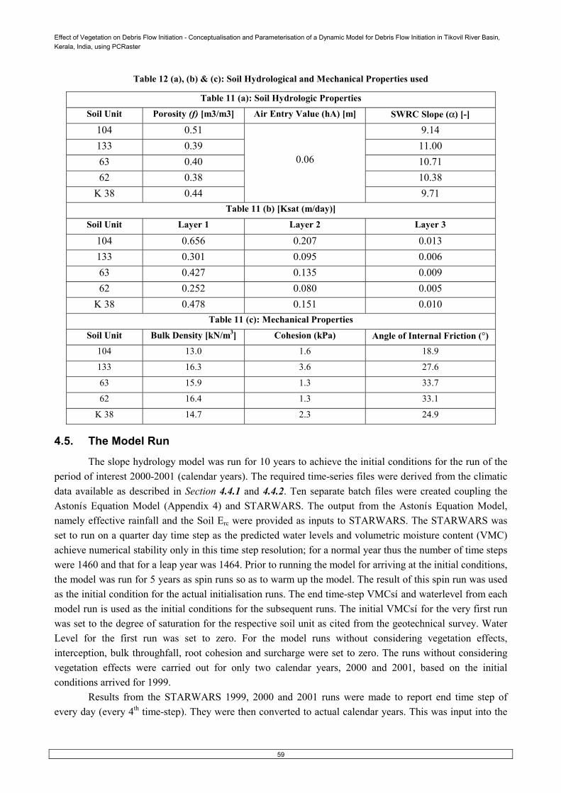
Effect of Vegetation on Debris Flow Initiation - Conceptualisation and Parameterisation of a Dynamic Model for Debris Flow Initiation in Tikovil River Basin, Kerala, India, using PCRaster
59
Table 12 (a), (b) & (c): Soil Hydrological and Mechanical Properties used
Table 11 (a): Soil Hydrologic Properties
Soil Unit Porosity (f) [m3/m3] Air Entry Value (hA) [m] SWRC Slope (α) [-]
104 0.51 9.14 133 0.39 11.00 63 0.40 10.71 62 0.38 10.38 K 38 0.44
0.06
9.71 Table 11 (b) [Ksat (m/day)]
Soil Unit Layer 1 Layer 2 Layer 3
104 0.656 0.207 0.013 133 0.301 0.095 0.006 63 0.427 0.135 0.009 62 0.252 0.080 0.005 K 38 0.478 0.151 0.010
Table 11 (c): Mechanical Properties Soil Unit Bulk Density [kN/m3] Cohesion (kPa) Angle of Internal Friction (°) 104 13.0 1.6 18.9
133 16.3 3.6 27.6
63 15.9 1.3 33.7
62 16.4 1.3 33.1
K 38 14.7 2.3 24.9
4.5. The Model Run
The slope hydrology model was run for 10 years to achieve the initial conditions for the run of the period of interest 2000-2001 (calendar years). The required time-series files were derived from the climatic data available as described in Section 4.4.1 and 4.4.2. Ten separate batch files were created coupling the Astonís Equation Model (Appendix 4) and STARWARS. The output from the Astonís Equation Model, namely effective rainfall and the Soil Erc were provided as inputs to STARWARS. The STARWARS was set to run on a quarter day time step as the predicted water levels and volumetric moisture content (VMC) achieve numerical stability only in this time step resolution; for a normal year thus the number of time steps were 1460 and that for a leap year was 1464. Prior to running the model for arriving at the initial conditions, the model was run for 5 years as spin runs so as to warm up the model. The result of this spin run was used as the initial condition for the actual initialisation runs. The end time-step VMCsí and waterlevel from each model run is used as the initial conditions for the subsequent runs. The initial VMCsí for the very first run was set to the degree of saturation for the respective soil unit as cited from the geotechnical survey. Water Level for the first run was set to zero. For the model runs without considering vegetation effects, interception, bulk throughfall, root cohesion and surcharge were set to zero. The runs without considering vegetation effects were carried out for only two calendar years, 2000 and 2001, based on the initial conditions arrived for 1999.
Results from the STARWARS 1999, 2000 and 2001 runs were made to report end time step of every day (every 4th time-step). They were then converted to actual calendar years. This was input into the

Effect of Vegetation on Debris Flow Initiation - Conceptualisation and Parameterisation of a Dynamic Model for Debris Flow Initiation in Tikovil River Basin, Kerala, India, using PCRaster
60
Effective Degree of Saturation Calculation Model based on Equation 2. The daily time step output of θeff and the Water Level output from STARWARS runs were input into the PROBSTAB model.
The PROBSTAB model was run in a batch file mode in order to arrive at the FOSM based Probabilities of Failure as described in Section 4.1.2. The batch file as well was made to report the sensitivity of the maps to the mechanical parameters of the model. The sensitivity maps were the difference maps of the Factor of Safety maps as derived using the First Positive Standard Deviation Maps and the First Negative Standard Deviation Maps. Other outputs from the model were, first day of instability, total number of days of instability, overall day of minimum safety factor and overall period of instability.
A preliminary run of STARWARS, indicated the necessity of calibration as per predicted observations in the eleven well locations for which water levels were measured during the fieldwork in the month of August 2005. So did PROBSTAB given no instability predicted at the very first instance for the reason of very high soil cohesion values as observed in Section 4.4.4.3, enabling to concluding that the cohesion tests were not conducted in standard test conditions. This necessitated the calibration of PROBSTAB.
4.5.1. The Model Calibration
Calibration was carried out based on the water levels predicted by STARWARS. Rainfall timeseries files for the years of 2004-2005 were used to predict the slope hydrology outputs for the respective years. The model was made to report water levels predicted at the eleven well locations for which field data was collected. Each parameter that contributes to water level was altered slightly and the model was rerun, each time with an altered value of a single parameter, thus several times. This indicated that the soil thickness was the one that had the most significant effect on the predictions. Given the uncertainty involved in mapping soil thickness, this was not a surprise. The soil thickness map was modified with slightly higher values and the model was rerun several times. The results are further discussed in Chapter 5.
Altering the mechanical properties and trying to match the predicted locations of slope instability with the observed landslide initiation locations prior to 1999 was how the calibration of slope instability model carried out. Cohesion and Root Cohesion being those with the most contribution to slope instability, values of these were tuned to match reality. Table 12 reports the values of all the parameters after selective calibration of the values.
In order to achieve the relative difference between the years 2000 and 2001, the parameters root induced cohesion and slope were varied for selective regions. The assumption underlying the calibration procedure was that the topography of the region is altered through contour bunding and other landuse practices and the DEM derived slope is not always the true representative. This being a localized fact, slope is a parameter that can be used for cohesion. Root induced cohesion a parameter that was estimated from empirical equations derived elsewhere also contains uncertainty, thus leaving room for using the parameter for calibration. Each time the values of one of these parameters were varied keeping all the other values constant. At a condition when the flow initiation locations were showing the desired factor of safety (FS<=1) during the known critical period, and the area shown unstable were relatively different, the calibration procedure was stopped. The values when altered beyond this stage, there was no significant improvement in the predictions and was seen varying without any correlation to the parameters altered.
4.5.2. Model Validation
Model validation was carried out with debris flow initiation locations and the hazard zonation map prepared by CESS. Validation of the flow initiation locations were carried out using the maps of debris flow initiation locations of 2000 (5 flows, dates unknown) and 2001 (11 flows, occurred on July 8th) by

Effect of Vegetation on Debris Flow Initiation - Conceptualisation and Parameterisation of a Dynamic Model for Debris Flow Initiation in Tikovil River Basin, Kerala, India, using PCRaster
61
comparing the predicted safety factors for the locations of debris flows. Temporal validation is carried out with the known debris flow occurrence date of 2001. If the model predicted that the known locations of flows were unstable during the critical period (South-West Monsoon) and specifically during the known day of occurrence of flows in the region, the model was assumed to be temporally validated for the purpose of this research.
Area validation of the derived probability of failure was carried out for the year 2001 in comparison with the hazard zonation map prepared by CESS. Assuming the hazard zonation map derived by CESS as a bench mark, the area of Probability of Failure with FS<=1 and the area classified as critical in the map was compared; the difference was considered as an index towards the performance of the model. A larger difference is because of underestimation or overestimation.
Table 13 shows the soil type, depth, slope and landuse of the flow initiation locations of 2000 and 2001. See Chapter 4, Table 12 for soil hydrological properties applicable to each soil type. See Chapter 3, Figure 18 & Figure 19 for the slide locations overlaid on Landuse Map and Drainage Map.
Table 13: Soil Type, Depth, Slope and Landuse characteristics of Flow Initiation Locations in 2000 and 2001
Year 2000 Location Code Soil Type Soil Depth Landuse Slope (%)
1 104 1.75 Grass and Rock 52 2 63 0.75 Rubber 68 3 104 1.25 Rubber 171 4 63 1.75 Rubber 64 5 63 1.75 Rubber 63
Year 2001 1 63 0.25 Rubber 103 2 63 0.25 Rubber 82 3 104 1.75 Grass and Rock 65 4 104 1.75 Rubber 12 5 104 3.50 Rubber 75 6 63 1.75 Forest Degraded 60 7 63 0.75 Forest Degraded 55 8 63 0.75 Grassland 63 9 63 0.75 Grassland 48 10 63 1.75 Rubber 70 11 63 0.25 Grassland 48

Effect of Vegetation on Debris Flow Initiation - Conceptualisation and Parameterisation of a Dynamic Model for Debris Flow Initiation in Tikovil River Basin, Kerala, India, using PCRaster
62
5. Results and Discussion
5.1. Parameterisation
Much effort was required to convert the accumulated data into the necessary parameters of the model as explained in Chapter 4. Results of this conversion from raw data to model parameters are discussed below.
5.1.1. Rainfall
Seasonal totals of Rainfall data for 31 years were available from CESS. As described in Chapter 4 Section 4.4.1 the rainfall seasonal totals for a period from 1965 to 1995 were used to calculate the initial conditions of slope hydrology for the model runs. Figure 30 shows the annual (hydrological years) rainfall recorded from 1965 to 1995. As explicit in the figure, 1981 experienced the highest total rainfall with a recorded figure of 6858.2 mm.
The annual totals, once the years are divided into hydrological years, have almost the same statistical distribution with the same peaks and troughs, but was more nearer to reality, as nature do not follow calendar years. The annual totals have an average of 5182.4 mm and a standard deviation of 829.6 mm. The deviation was reduced, as the annual calendar totals are converted to hydrological year totals; the average is 5181.0 mm and the standard deviation 762.3 mm. By considering hydrological years for analysis, the overall deviation of rainfall from normal was reduced, but without sacrificing the variability of rainfall across years.
Figure 30: Rainfall of Hydrological Years in the study area from 1965 to 1995
0
1000
2000
3000
4000
5000
6000
7000
1 3 5 7 9 11 13 15 17 19 21 23 25 27 29
Years
Rainfall (in
mm)
Hydrological Year
The daily variability of rainfall in a hydrological leap year and normal year as deduced from the data of 2000-2001 were used for creating the daily rainfall time-series for the model runs (Explained in Chapter 4 Section 4.4.1). The variability of rainfall is presented in Figure 31.

Effect of Vegetation on Debris Flow Initiation - Conceptualisation and Parameterisation of a Dynamic Model for Debris Flow Initiation in Tikovil River Basin, Kerala, India, using PCRaster
63
Figure 31: Daily Variability of Rainfall in Hydrological Leap year and Normal year based on 2000-2001 data
0
50
100
150
200
250
1 41 81 121 161 201 241 281 321 361Julian Days (Hydrological)
Rainfall (in mm)M
HY P - leap HY P - normal
Daily rainfall deduced for each year from the seasonal totalsí of the respective year follow this trend, depending on whether it is a leap year or a normal year. The trend for the leap year has the maximum spike on the 38th day (July 8th) and there are three preceding spikes that gradually rise to reach the peak. Significance of these spikes is evident when read in conjunction with the fact that there were 11 reported debris flows that occurred on 8th July 2001.
For a period from the 190th day to the 268th day, there is a persistent lack of rainfall irrespective of whether it is a normal year or a leap year. The period is crucial as the relative dryness of soil that sets in during this period is crucial to the overall stability of the region, providing some time for the soil to compact itself. Interim rainfall events during this period ensure sufficient residual moisture to keep the soil in cohesive conditions that ensure stability.
5.1.2. Potential Evapotranspiration
Average daily PET for the study area based on computed values of PET using Equation 19 with data for 2000-2001 was 4.38 mm/day with a Standard Deviation of 0.65. Figure 32 shows the calculated evapot ranspi rat i on for the actual hydrol ogi cal year 2000 (J une 1st 2000 - May 31st 2001) and for the hypothetical Dry Days Year and Wet Days Year calculated as described in Chapter 4 Section 4.4.2. It is evident from the graph that the actual hydrological year values had considerable extreme values, which is reduced by recomputing it for the hypothetical dry-days-year and wet-days-year. The general trend is preserved and so is the variability, but occurrence of extreme Erc values on wet days are avoided.

Effect of Vegetation on Debris Flow Initiation - Conceptualisation and Parameterisation of a Dynamic Model for Debris Flow Initiation in Tikovil River Basin, Kerala, India, using PCRaster
64
Figure 32: Potential Evapotranspiration of 2000-2001 and hypothetical years
0.00
1.00
2.00
3.00
4.00
5.00
6.00
7.00
1 26 51 76 101 126 151 176 201 226 251 276 301 326 351
Dry Days Year Wet Days Year 2000-2001
5.1.3. Interception
Daily interception was calculated using Astonís Equation (Equation 2 and Appendix 4). Figure 35 shows the monthly average interception maps computed for June 2001 to December 2001. In order to decide the most suitable method for calculating fractional vegetation cover (fc) from NDVI, three methods were attempted. The attempts and the relative variations are reported in Sekhar et al., (In Press) (Extended Abstract provided as Appendix 5). Figure 33 shows the relative differences of fc computed from three methods for the moths from June to December 2001. Monthly average values of sixty-two randomly chosen pure vegetation pixels across peninsular India were used to derive the graphs. From the graph it is evident that fc computed using the conventional method was not at all acceptable for its overestimation of fractional vegetation cover owing to the spurious pixels problem; Gutman method provided acceptable results and also the trend was nearer to that of Walthall method derived fc with a kc value of 0.8. However, the advantage of Walthall et al., (2004) method being it more sensitive to actual vegetation types on ground makes it the most ideal choice. The graphs prepared using a kc value of 0.2 and 0.8 indicates the sensitivity of this method to the crop coefficients and thus the actual condition of ground cover.
The fractional vegetation cover computed has significantly low values in the month of August. Reason for this was the poor quality of the MODIS derived NDVI data owing to the severe cloud cover conditions prevailing in the region. October data also has some cloud cover and thus the available composite NDVI data is not of the best quality. The relationship of fc to LAI being logarithmic, the values though will not provide the most realistic result but will provide a good estimate of LAI, useful for computing the subsequent parameters. As the parameters were not used for model fitting, the results were reasonable enough for the research as observed later in the study.

Effect of Vegetation on Debris Flow Initiation - Conceptualisation and Parameterisation of a Dynamic Model for Debris Flow Initiation in Tikovil River Basin, Kerala, India, using PCRaster
65
Figure 33: Comparison of Fractional Vegetation Cover computed using different methods
0.00
0.20
0.40
0.60
0.80
1.00
1 2 3 4 5 6 7
Months
Fractional Vegetation Cover (-) m
Gutman Conventional Walthall (0.2) Walthall (0.8)
The maps indicate acceptable interception rates during the entire monsoon season, June being the first month of rainfall; leaf area being less due to preceding summer leading to a lesser amount of interception. As rainfall continues, Interception rates also increase owing to leaf growth. It can be seen that the non-rubber areas (See Figure 13, Chapter 2) do not show much variation. Rubber being a deciduous plant blooms with leaf growth during the rainy season, thus increasing the interception rates as rainy days progress. By the month of December most of the rubber plants are left with significantly less number of leaves and thus results in reduced rates of interception, also evident from the map indicating very low interception rates during the month.
Figure 34 shows the interception calculated at two difference debris flow initiation locations during the year 2001. It can be seen that there is a relative variation in the graph but the trend remains the same. The reason for variation is the amount of canopy cover present in each location and the reason for same trend being the seasonal variation in canopy cover.
Figure 34: Interception at two locations for the calendar year 2001
(b): Calendar Year 2001
0.00
1.00
2.00
3.00
4.00
1 46 91 136 181 226 271 316 361
Julian Days
Interception (mm)
Location 2 Location 3

Effect of V
egetation on Debris Flow
Initiation - Conceptualisation and P
arameterisation of a D
ynamic M
odel for Debris Flow
Initiation in Tikovil River B
asin, Kerala, India, using P
CRaster
66
Figure 35: Average M
onthly Interception Maps

Effect of Vegetation on Debris Flow Initiation - Conceptualisation and Parameterisation of a Dynamic Model for Debris Flow Initiation in Tikovil River Basin, Kerala, India, using PCRaster
67
The advantage of such an approach to parameterisation of interception was that it helps to avoid crisp boundaries of defined landuse classes. So also, interception, a phenomenon with established relationships to the leaf area (Walthall et al., 2004), which in turn is related to the seasonal variations of vegetation development, has considerable spatial variation; a fact proved from the maps. Not every tree even in a plantation will have the same leaf development and thus will induce different rates of interception. Interception thus has intra-class spatial variability and inter-class spatial variability, both of which are accounted using the approach adopted in the research. This approach also agrees to the conceptual schema put forth in Paragraph 8 Section 5.1 and thus an improvement to the traditional approach towards hydrological model parameterisation.
The simulation clearly indicates that rubber plantations induce the highest amount of interception for any given rainfall event reaching a maximum value of about 5 mm at places on a daily time-step. Mixed crops follows with about 3 to 4 mm. Tea Gardens tend to induce very little interception, while grasslands inducing none.
However, as the REA chosen for modelling is 20 m by 20 m and that the landuse map was available in that resolution, by utilizing the above stated approach inevitable generalisation has cropped in because of the original 250 m by 250 m resolution of the NDVI dataset. It is also true that no field estimates of interception were available. Most of the area being rubber grown and also the fact that most of the debris flows occurred in rubber grown areas, if crisp datasets were used, the relative variability of interception would not have had been accounted. By utilizing the approach stated, both spatial and temporal variability of the parameter could be incorporated. Increasing spatial resolutions and the possibility of multi sensor approach towards the derivation of NDVI datasets (and thus achieve much better temporal coverage) lights a promising path towards parameterising such models using satellite datasets.
5.1.4. Effective Rainfall and Bulk Throughfall Time-series Maps
Effective rainfall is the total, unintercepted gross rainfall that reaches the soil surface and is available for infiltration. It thus comprises throughfall and all intercepted rain in excess of the maximum interception storage capacity.
Bulk throughfall (BT) coefficient was computed using Equation 6. Figure 36 shows the Average Bulk Throughfall Coefficient maps computed for the years 2000 and 2001. Average bulk throughfall coefficient of the region based on computed monthly bulk throughfall coefficients for the years 2000 and 2001 (excluding January 2000) was 0.31, with the highest value reached being 0.58. This implies that on an average 31% of the total intercepted rainfall reaches the surface as bulk throughfall.
Though the BT was derived only on a monthly basis, it is applied on the daily time-step simulation of slope hydrology resorting to the assumption of equal bulk throughfall for all the rainfall events (total rainfall in a day) occurring in a month. Though this abstraction and resultant parameterisation has its own limitations (as bulk throughfall like interception varies from event to event depending on the average raindrop size and intensity) it has the same advantages as that of interception elaborated in Section 5.2.3.
Effective rainfall was computed by reducing the amount of rainfall in a day with the interception. Bulk throughfall was accounted and so a certain amount of intercepted rainfall will further flow down as BT and add to the rainfall reduced with interception. In order to account for areas with and without vegetation cover the reduction in rainfall was achieved through the following Equation 23.
)0))),,0max(*)1(()*((,0( iiieff SRFBTRFBTRFifRF −−+>=
Model implementation of Effective Rainfall: [23]

Effect of Vegetation on Debris Flow Initiation - Conceptualisation and Parameterisation of a Dynamic Model for Debris Flow Initiation in Tikovil River Basin, Kerala, India, using PCRaster
68
where, RF is Rainfall in a given time-step, BT the bulk throughfall coefficient and Si the interception at that particular time-step.
Assume a hypothetical rainfall of 10 mm on a pixel with vegetation inducing a BT of 0.2 and Si of 4 mm, the effective rainfall will be: 2 + (0.8*6) = 6.8 mm
Assume that the same amount of rain, falls in a pixel devoid of vegetation and thus having no BT and no Si, the effective rainfall will be: 0 + (1*10) = 10 mm
Using the above approach rainfall of every time-step was reduced to the corresponding net rainfall. Maximum reduction is observed in areas of rubber plantation owing to the broad leafs of the tree facilitating larger amounts of storage and thus relatively greater amounts of interception.
5.1.5. Soil Erc Time-series Maps
PET computed using Equation 19 was reduced to the amount of PET that needs to occur from Soil using a similar approach as that of Effective Rainfall. The equation used was:
))0),0,max(,0,0(*)1(()*( iCumirc SPETPETRFifBTPETBTSoilE −+>−+= Model implementation of Soil Evapotranspiration: [24]
where, Soil Erc is the remnant of PET to occur from soil, BT is Bulk throughfall coefficient, RF is Rainfall of a given time-step, PETCum the cumulative PET up till the given time-step and Si the interception.
Assume a pixel with PET of 10 mm, BT of 0.2, Rainfall of 10 mm and Interception of 5 mm (which implies that there is vegetation cover) and assume that it is the first time-step and so ErcCum is 0. Soil Erc will be: 2 + 0 = 2 mm.
Assume the same day without rainfall then PET will be different and let it be 11 mm (See Section 5.3 for reasons of different PET values); Soil Erc will be: 2.2 + (0.8*6) = 7 mm.
If the pixel is devoid of vegetation and thus no interception and no BT, but with a rainfall of 10 mm and PET of 10 mm, Soil Erc will be 10 mm and the rainfall is passed on to the soil unhindered. Assume the same scenario with no rainfall and thus PET of 11 mm; then Soil Erc will be 11 mm.
As was the case with Effective Rainfall, rubber plantations induce maximum reduction. Figure 37 shows the Soil Erc to occur on 7th July and 8th July 2001. Though both the days were rainy, as the previous time-steps had accumulated evapotranspiration, a certain amount of net rainfall is still evapotranspired before being available for soil hydrological processes. The plateau region of the study area shows very little amount of Soil Erc and the valley portions mostly covered with rubber and relatively thicker soils show higher rates of evapotranspiration. Remnant of PET to occur from soil for the whole study area was thus calculated and provided as input to STARWARS for prediction of slope hydrology. The potential rate was later corrected to the respective actual values for each landuse using the crop coefficients.

Effect of V
egetation on Debris Flow
Initiation - Conceptualisation and P
arameterisation of a D
ynamic M
odel for Debris Flow
Initiation in Tikovil River B
asin, Kerala, India, using P
CRaster
69
Figure 36: Average A
nnual Bulk Throughfall C
oefficient

Effect of V
egetation on Debris Flow
Initiation - Conceptualisation and P
arameterisation of a D
ynamic M
odel for Debris Flow
Initiation in Tikovil River B
asin, Kerala, India, using P
CRaster
70
Figure 37: Soil Evapotranspiration of 7th and 8th July 2001

Effect of Vegetation on Debris Flow Initiation - Conceptualisation and Parameterisation of a Dynamic Model for Debris Flow Initiation in Tikovil River Basin, Kerala, India, using PCRaster
71
5.1.6. Root Induced Cohesion and Surcharge
From initial calculations it was observed that the root-induced cohesion calculated with tensile strengths for the 7 year old plant and 23 year old plant did not vary much. The reason for both being similar can be attributed to the fact that the size of roots tested was more or less similar, owing to the non availability of appropriate machinery to carryout the task for smaller roots. The average root induced cohesion across different soil types and soil thickness units is 9.8 kPa assuming that the whole rubber grown area was covered with 23 year old rubber trees and it is 6.54 kPa if it were 7 year old rubber plants. It was observed during the field work that currently most of the study area is producing latex, implying that the region mainly has matured rubber trees. So the values pertaining to 23 year old rubber plant was used to compute root-induced cohesion. The method adopted for root cohesion estimation is the simplest and thus pragmatic for quick parameterisation of a numerical model to provide reasonable results.
Based on the measured tensile forces (Table 14) for the three root samples, tensile strength of a 5 mm root was estimated.
Table 14: Root Sample - Diameters and Tensile Strength Root Diameter (mm) Root Tensile Strength (kPa)
90 2483.6 120.5 1420.5 160 895.25
The relationship between root diameter and root tensile strength (Figure 38) was used to derive the tensile strength of a 5 mm root. Though the derived results were used for the modelling, it is for sure that the extrapolation induced significant overestimation in the resultant values. Assuming no trend the error involved in the extrapolations was phenomenal. However, as no better measures were possible within the scope of the present work, the use of extrapolated values were inevitable.
Figure 38: Root Diameter-Root Tensile Strength Relationship
y = 8727e-0.0144x
0.00
500.00
1000.00
1500.00
2000.00
2500.00
3000.00
80 100 120 140 160 180
Root Diameter (mm)
Root Tensile Strenght (kPa)
Root counts derived from the pit were used to extrapolate for root counts at various soil depths (Figure 39). The graph shows a progressive reduction in the number of roots present in each soil depth class, which is in near agreement to the trend computed by Srinivasan et al, (2004).

Effect of Vegetation on Debris Flow Initiation - Conceptualisation and Parameterisation of a Dynamic Model for Debris Flow Initiation in Tikovil River Basin, Kerala, India, using PCRaster
72
Figure 39: Root Counts at various Soil Depths
0
100
200
300
400
500
600
0.00
0.50
1.00
1.50
2.00
2.50
3.00
3.50
4.00
4.50
5.00
Soil Depth (m)
Root Count
Given the root counts at various soil depths and the reasonably assumed value of average root diameter, the root cross sectional area at each soil depth class was derived assuming that every root face is circular. Root cross sectional area for a given soil depth class is the area of each root face (πr2) multiplied with the root counts corresponding to that particular class. Tensile Strength is then root cross-sectional area multiplied by the root tensile strength of the 5 mm root (8120.7 kPa). Field derived angle of shear measured 21.3° and the angle of internal friction for each soil type was used to computed the value of ëaí. Values of tensile strengths corresponding to each soil depth class falling in each of the soil type unit were multiplied with the ëaí value for the particular soil type. It is reiterated that root induced cohesion was computed only for the rubber grown area. Figure 40 shows the additional cohesion induced by roots along various soil depth classes for each soil type. The graphs agree to the general understanding of root-induced cohesion as reducing with soil depth.
Figure 40: Root Induced Cohesion as it varies with Soil Depth for each Soil Type
0.00
10.00
20.00
30.00
40.00
50.00
60.00
1 2 3 4 5 6 7 8
Soil Depth (m)
Root Induced Cohesion (kPa)
RC Soil Unit 63 RC Soil Unit 104 RC Soil Unit 133
RC Soil Unit 62 RC Soil Unit KSLUB

Effect of Vegetation on Debris Flow Initiation - Conceptualisation and Parameterisation of a Dynamic Model for Debris Flow Initiation in Tikovil River Basin, Kerala, India, using PCRaster
73
Figure 41 shows the calculated root-induced cohesion as varying with soil depths and soil types for the rubber grown area.
Figure 41: Root Induced Cohesion
The computed value of surcharge was 0.27 kPa. This value was assumed to be applicable for the
entire rubber grown area relying on the same assumption as that for root induced cohesion, that the entire rubber grown area is covered by matured rubber plants. This assumption was necessitated by the non availability of weight measurements of younger rubber plants. Even if such measurements were available, unless until a landuse map depicting the age classes of rubber trees are not available, it is of no practical use in the modelling activity.
5.1.7. Soil Thickness Map
Soil thickness map was one of the most important inputs in the numerical model. A fairly good estimation of soil depth was available. Figure 42 shows the soil thickness map used for the modelling. The depth varies from 0 to 5 m; zero depth for rock exposures and 5 m at some valley bottoms. Table 10 in Chapter 4 Section 4.3.3.4 details the area statistics of various soil thickness units. Correlation between soil thickness map and slope indicates that they are moderately correlated with a correlation coefficient of 0.51. Mean soil thickness of the area is 0.35 m with a standard deviation of 0.66. Lack of perfect correlation can be attributed to the abstraction of actual and interpolated values to classes in the original data and further abstraction to unit scalar values for model parameterisation. Several authors (DeRose et al., 1991; Odeh et al., 1991) have reported that soil depth is highly correlated to slope and/or landform units. In the most idealistic situation soil depths are to be finely sampled, interpolated and adjusted to landform characteristics and subsequently slope of the region. In conditions were data is deficient, given few estimates of soil

Effect of Vegetation on Debris Flow Initiation - Conceptualisation and Parameterisation of a Dynamic Model for Debris Flow Initiation in Tikovil River Basin, Kerala, India, using PCRaster
74
depths, it is plausible to derive a soil thickness map with a known relationship for a similar terrain elsewhere, reported by researchers.
The slope hydrology model calibration was carried out using the soil thickness map. After a number of iterations (done manually) a value of 0.08 m was arrived at. This value was added to all the soil units excluding the rock exposures and thus acceptable results were derived from the slope hydrological model. See the next section for the results of the calibration.
Figure 42: Soil Thickness Map
5.2. Model Run
Time utilization of STARWARS was significantly high owing to the parameterisation based on satellite data. Each map was about 1.5 Mb with 656 rows and 606 columns. In a Pentium 4, 1.8 Ghz processor CPU, supported with a 512 Mb DDR RAM, every time-step required about 7 seconds. Five continuous days of computing was required to arrive at the initial conditions for the actual runs of 2000 and 2001. The slope stability model required just about 1 sec for every time-step. In general, both the models are processor intensive and necessitate fast desktop computers to be time efficient.

Effect of Vegetation on Debris Flow Initiation - Conceptualisation and Parameterisation of a Dynamic Model for Debris Flow Initiation in Tikovil River Basin, Kerala, India, using PCRaster
75
5.3.1. STARWARS Results
The model was initially set to run for the years of 2004-2005 and 2005-2006. The data for 2006 was synthetic for completeness of the 2005-2006 time-series. The result from this run was used to calibrate the model based on the one time observation available for the month of August of 2005. It is relevant to note that the branch of Central Ground Water Department functioning in the state was not cooperative and did not provide ground water monitoring data that they regularly collect for the region from various wells thus reducing the scope of calibration to a single day of field measurement for 11 well locations in the study area during the peak monsoon season. Figure 43 shows the predictions of ground water made by STARWARS before and after calibration the respective correlations between the observed and predicted.
Figure 43: Relationship between Observed and Predicted Water Levels for 2005
After Calibrationy = 0.9967xR2 = 0.7043
Before Calibrationy = 0.9432xR2 = 0.7008
0.000.200.400.600.801.001.201.401.601.802.00
0.00 0.50 1.00 1.50 2.00
Observed Water Level (m)
Predicted Water Level (m)
Before Calibration After CalibrationLinear (After Calibration) Linear (Before Calibration)
The eleven well locations were widely distributed in the study area with no wells present in the plateau. As two of the well locations were in valley points, the model predicted significantly high and persisting water levels at these locations. So these locations were avoided from being used for calibration. The observed and predicted water levels for the month of August (assuming that the observation made in the field for 10th of August 2005 as the average for the whole month) were seen to have moderately high correlation for the remaining nine well locations. In order to arrive at satisfactory results, the model was tuned with an addition of 0.08 meter to all the soil thickness classes excluding the rock exposures, the model predicted acceptable results. It can be seen that not only did the R2 improve as a result of calibration, but also did the intercept, which was 0.9432 prior to the calibration and 0.9967 after the calibration.
Once calibrated with the available reference data, the model was set for 5 years (with 1989 rainfall time-series) of spin runs. The end day result of this spin run was used to run for the 11 initialization years (1989 ñ 1999 hydrological years). The results of the last day of 1999 was reported and used to run 2000 and the 2000 results to run 2001. Results from STARWARS (volumetric moisture content and waterlevels) were used to calculate the effective degree of saturation. The results for hydrological years 1999, 2000 and 2001 of effective degree of saturation and waterlevels, were converted to actual calendar years of validation, 2000 and 2001. Figure 44 shows the predicted maximum water levels with the effects of vegetation on

Effect of Vegetation on Debris Flow Initiation - Conceptualisation and Parameterisation of a Dynamic Model for Debris Flow Initiation in Tikovil River Basin, Kerala, India, using PCRaster
76
hydrology for the hydrological years 2000 and 2001 and Figure 45 shows the predicted maximum effective degree of saturation for the same period.
The map clearly indicates that waterlevels and effective degree of saturation generated in the region are more or less the same during the validation years. The predictions do not show any difference with and without vegetation effects on hydrology. Figure 46 (a) & (b) shows the predicted waterlevels, considering vegetation effects, at 2 of the 5 flow initiation locations in 2000 and 2 of the 11 initiation locations in 2001, respectively. Points are chosen so as to show the relative spatial variability in predictions for the respective years. Though there are instantaneous changes in the waterlevels predicted by the model, with and without vegetation effects, the maximum waterlevels are more or less the same. In the year 2000, Location 1 & 4 of 2000 had the maximum waterlevel of 1.83 m and in the year 2001, Location 5 of 2001 had the highest waterlevel of 3.5 m. Table 15 provides the minimum, maximum, average and standard deviation of the predicted waterlevels at the flow initiation locations of 2000 and flow initiation locations of 2001. From Table 16 it can be seen that the on the known day of flow initiation the waterlevels were at its peak.
5.3.2. Sensitivity of STARWARS
Table 16 provides the simulated hydrological effects and transient hydrological conditions of July 8th 2001 for the flow initiation locations of 2001. The data in the table indicates that though the region has significant vegetation cover the interception effect is negligible. The model computed that canopy interception results in less than 1% reduction of the primary rainfall of July 8th 2001 at the flow initiation locations. The reason for this can be attributed to the practical insignificance of interception in tropical climates, as observed by several researchers on the topic (Calder, 2001; Jorge and Sharika, 2000). In tropics large drop sizes in the primary rainfall and large drop sizes in secondary drops falling from vegetation helps to explain why in absolute and relative terms interception loss from tropical tress is less than that in temperate climates (Calder, 2001).
The next important parameter to be considered while discussing about vegetation effects on slope hydrology is the evapotranspiration. The potential value was reduced with the respective crop factors for each landuse type and the net rainfall reaching the surface is reduced with the calculated actual evapotranspiration value. The resultant amount of water is available for the soil hydrological processes. As Bulk Throughfall is considered in the model, though July 8th 2001 is a rainy day, as there is a certain amount of water in the soil, evapotranspiration occur from the soil at a reduced rate (See Chapter 4, Section 4.4.2 for the rainy and dry day PET calculations used). As this amount is as well not very significant in the study area, the waterlevels generated are not much affected by the hydrological effects of vegetation. From a total rainfall of 237.8 mm of rainfall per pixel, only 3.67 mm is evapotranspired, on July 8th 2001. It also corroborates the observations made in the research works in tropical climatic conditions that, on rainy days the evapotranspiration is practically negligible (Nizinski et al., 1994; Watanabe et al., 2004).
Though both interception and evapotranspiration does not seem to have significant influence on a daily basis, they still have relevance in maintaining the long term saturation conditions of the soil. This explains the delay in the occurrence of debris flows even when the factor of safety is well below 1 several days prior to the actual date.
The effective degree of saturation is not related to the depth, but is an indication of the amount of unsaturated zone filled with water. In theory, if a soil layer is with zero waterlevel and zero effective degree of saturation, it implies that the layer is completely dry. In the present study it was observed that the effective degree of saturation was at the lowest on the slide day, but waterlevels at its peak. It was also observed that with the decreasing depth of the unsaturated zone, the percolation was rapid and thus drained

Effect of Vegetation on Debris Flow Initiation - Conceptualisation and Parameterisation of a Dynamic Model for Debris Flow Initiation in Tikovil River Basin, Kerala, India, using PCRaster
77
off more water than expected. This is a clear numerical inconsistency. With the given datasets it was not possible to rectify it in a short time, though efforts to this end were taken up. Nevertheless, waterlevel is the dominant factor and it is well included in the model.
The inconstancies in the slope hydrology predictions can be attributed to the lack of consistent data sets. So also it needs much more time consuming adaptations of the model and further calibration efforts with congruent data sets to make the model predict the reality much more clearly in a the tropical monsoon conditions of Kerala.
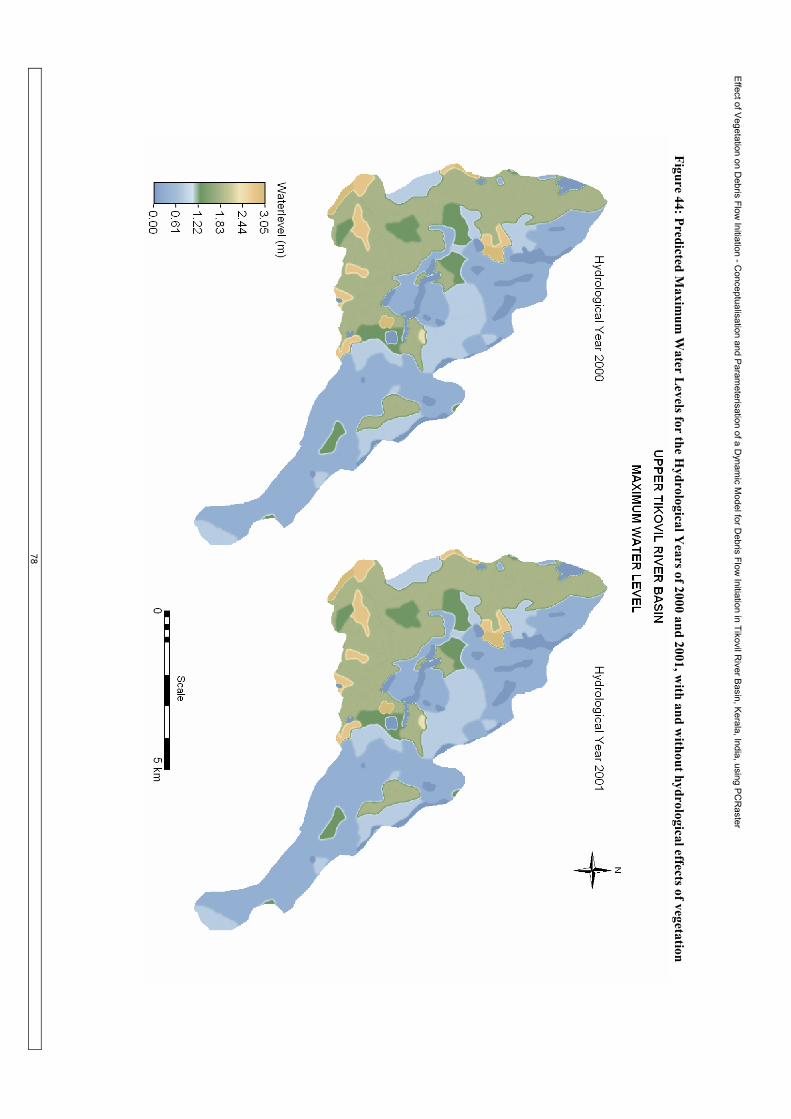
Effect of V
egetation on Debris Flow
Initiation - Conceptualisation and P
arameterisation of a D
ynamic M
odel for Debris Flow
Initiation in Tikovil River B
asin, Kerala, India, using P
CRaster
78
Figure 44: Predicted Maxim
um Water Levels for the H
ydrological Years of 2000 and 2001, w
ith and without hydrological effects of vegetation

Effect of V
egetation on Debris Flow
Initiation - Conceptualisation and P
arameterisation of a D
ynamic M
odel for Debris Flow
Initiation in Tikovil River B
asin, Kerala, India, using P
CRaster
79
Figure 45: Predicted Maxim
um Effective D
egree of Saturation for the Hydrological Y
ears of 2000 and 2001, with hydrological effects of vegetation

Effect of Vegetation on Debris Flow Initiation - Conceptualisation and Parameterisation of a Dynamic Model for Debris Flow Initiation in Tikovil River Basin, Kerala, India, using PCRaster
80
Table 15: Minimum, Maximum, Average and Standard Deviation of Predicted Water Levels (considering vegetation effects) at the 2000 and 2001 Flow Initiation Locations and Soil Depths at the locations LC Minimum Maximum Average STDEV Soil Depth
Year 2000 1 0.00 1.83 0.79 0.75 1.75 2 0.00 0.63 0.16 0.25 0.75 3 0.00 1.13 0.26 0.42 1.25 4 0.00 1.83 0.52 0.70 1.75 5 0.00 1.53 0.43 0.59 1.75
Year 2001 1 0.00 0.33 0.14 0.15 0.25 2 0.00 0.29 0.12 0.13 0.25 3 0.00 1.80 1.02 0.73 1.75 4 0.00 1.83 0.83 0.81 1.75 5 0.00 3.20 1.38 1.34 3.50 6 0.00 1.83 0.87 0.79 1.75 7 0.00 0.82 0.35 0.37 0.75 8 0.00 0.81 0.31 0.35 0.75 9 0.00 0.82 0.33 0.36 0.75 10 1.24 1.83 1.82 0.03 1.75 11 0.00 0.32 0.19 0.15 0.25
STDEV: Standard Deviation; LC: Location Code
Table 16: Simulated Slope Hydrology for July 8th 2001 at the Flow Initiation Locations of 2001, with and without considering vegetation effects
LC RF (mm)
Ic (mm)
BT (-)
ERF V
(mm)
ERF NV (mm)
WL V (m)
WL NV (m)
EDS V (-)
EDS NV (-)
1 2.4 0.54 236.4 0.33 0.33 2 2.3 0.54 236.5 0.29 0.30 3 0.4 0.00 237.8 1.80 1.80 4 1.0 0.41 237.3 1.83 1.83 5 0.9 0.00 237.8 3.20 3.20 6 1.5 0.53 237.0 1.83 1.83 7 1.2 0.15 237.6 0.82 0.84 8 0.6 0.00 237.8 0.81 0.80 9 0.7 0.10 237.7 0.82 0.85 10 1.2 0.40 237.3 1.83 1.83 11
237.75
0.6 0.00 237.8
237.75
0.32 0.33
0.001
0.001
LC: Location Code; RF: Rainfall; ERF: Effective Rainfall; Ic: Interception BT: Bulk Throughfall Coefficient; WL: Water Level; EDS: Effective Degree of Saturation V: Considering Vegetation; NV: Without Considering Vegetation

Effect of V
egetation on Debris Flow
Initiation - Conceptualisation and P
arameterisation of a D
ynamic M
odel for Debris Flow
Initiation in Tikovil River B
asin, Kerala, India, using P
CRaster
81
Figure 46 (a & b): W
ater Levels predicted for two Debris Flow
Initiation Locations each, considering Vegetation Effects for the years 2000 &
2001
(a): Calendar Year 2000
0.00
0.50
1.00
1.50
2.00
146
91136
181226
271316
361
Julian Days
Water Level (m)Location 1
Location 5
(b): Calendar Year 2001
0.00
0.50
1.00
1.50
2.00
146
91136
181226
271316
361
Julian Days
Water Level (m)
Location 2Location 3

Effect of Vegetation on Debris Flow Initiation - Conceptualisation and Parameterisation of a Dynamic Model for Debris Flow Initiation in Tikovil River Basin, Kerala, India, using PCRaster
82
5.3.3. PROBSTAB Results
PROBSTAB was set to run for the calendar years of 2000 and 2001. The run was carried out with and without hydrological and mechanical effects of vegetation. The difference between the results was interesting; in the former case, the area predicted as unstable (FS<=1) were relatively very less when compared to the results of the later. Figure 47 (a) & (b) shows the overall stability of the region based on the minimum safety factor scored on each pixel for the respective years and Figure 49 (a) & (b) shows the daily variations in safety factors at the flow initiation locations of 2000 and 2001 respectively, computed considering vegetation influence. Unstable areas are those with FS<=1. Table 17 shows the minimum, maximum, average and standard deviation of safety factor predicted at the known flow initiation locations of 2000 and 2001, with the vegetation effects considered. Figure 48 shows the daily changes of slope instability in 2000, as displayed by the PCRaster dynamic visualisation. It can be seen that the region in general is stable excluding some small portions. Instability sets in from some where around the Julian day of 216 and is also visible on 284th day. In theory, a deterministic model for debris flow initiation can be said to perfectly predicting the temporal occurrence of an event when the first day of predicted instability matches with the day of occurrence of slides. In the present study, this was not the case; given the fact that the region experiences short periods of high waterlevels the maximum pore pressure conditions are reached quiet often (see Figure 46). When approached from a deterministic perspective, thus the region appears to fail every now and then, when a critical rainfall amount is crossed. This fails deterministic models to capture the reality of temporal occurrence with a perfect match. But the study indicates that this does not make deterministic modelling attempts invalid for the region. Comparing the safety factor graphs for 2000 and 2001 reveals that in 2001, the region experienced a longer term of instability conditions than 2000 before the final failure on July 8th 2001. On an average, the known flow initiation locations of 2000 experienced 26 unstable days, till July 8th 2000; whereas in 2001 the known flow locations experienced 81 unstable days till July 8th 2001. Overall difference of number of days of instability also explains the reason for a larger number of events in 2001. In 2000 there were only 101 unstable days whereas in 2001 it was 186.

Effect of V
egetation on Debris Flow
Initiation - Conceptualisation and P
arameterisation of a D
ynamic M
odel for Debris Flow
Initiation in Tikovil River B
asin, Kerala, India, using P
CRaster
83
Figure 47 (a) & (b): O
verall Stability of the study area in 2000 and 2001, considering vegetation effects

Effect of V
egetation on Debris Flow
Initiation - Conceptualisation and P
arameterisation of a D
ynamic M
odel for Debris Flow
Initiation in Tikovil River B
asin, Kerala, India, using P
CRaster
84
Figure 48: Daily V
ariations of Safety Factor in 2000 as visualized in PCRaster
Day 1
Day 36
Day 216
Day 284
Day 320
Day 366

Effect of Vegetation on Debris Flow Initiation - Conceptualisation and Parameterisation of a Dynamic Model for Debris Flow Initiation in Tikovil River Basin, Kerala, India, using PCRaster
85
Figure 49 (a & b): Daily Variation of Safety Factor for 2000 and 2001, considering Vegetation Effects
(a): Calendar Year 2000
0.0
0.5
1.0
1.5
2.0
1 46 91 136 181 226 271 316 361
Julian Days
Safety Factor (-)
Location 1 Location 2 Location 3 Location 4 Location 5 FS=1
(b): Calendar Year 2001
0.0
0.5
1.0
1.5
2.0
1 46 91 136 181 226 271 316 361Julian Days
Safety Factor (-)
Location 1 Location 2 Location 3 Location 4 Location 5 Location 6
Location 7 Location 8 Location 9 Location 10 Location 11 FS=1

Effect of Vegetation on Debris Flow Initiation - Conceptualisation and Parameterisation of a Dynamic Model for Debris Flow Initiation in Tikovil River Basin, Kerala, India, using PCRaster
86
Figure 50 (a & b): Daily Variation of Safety Factor for 2000 and 2001, without considering Vegetation Effects
(b) Calendar Year 2000
0.00
0.50
1.00
1.50
2.00
1 46 91 136 181 226 271 316 361
Julian Days
Safety Factor (-)
Location 1 Location 2 Location 2 Location 3 Location 4Location 5 FS=1
(b): Calendar Year 2001
0.00
0.50
1.00
1.50
2.00
1 46 91 136 181 226 271 316 361
Julian Days
Factor of Safety (-)
Location 1 Location 2 Location 3 Location 4Location 5 Location 6 Location 7 Location 8Location 9 Location 10 Location 11 FS=1

Effect of Vegetation on Debris Flow Initiation - Conceptualisation and Parameterisation of a Dynamic Model for Debris Flow Initiation in Tikovil River Basin, Kerala, India, using PCRaster
87
Table 17: Minimum, Maximum, Average and Standard Deviation of Safety Factor (considering vegetation effects) at the 2000 and 2001 Flow Initiation Locations
Location Code Minimum Maximum Average STDEV Year 2000
1 0.82 1.12 0.97 0.11
2 1.29 1.61 1.50 0.11
3 0.87 1.40 1.25 0.19
4 0.97 1.30 1.16 0.11
5 0.97 1.27 1.15 0.10
Year 2001
1 1.10 1.10 1.07 0.03
2 0.97 1.03 1.01 0.03
3 0.86 1.06 0.95 0.08
4 0.77 1.02 0.89 0.10
5 0.87 1.07 0.97 0.07
6 0.91 1.20 1.05 0.12
7 0.93 1.22 1.09 0.13
8 0.97 1.24 1.12 0.12
9 0.91 1.23 1.09 0.14
10 2.90 3.03 2.90 0.01
11 0.95 1.03 0.98 0.03
Though the model could not provide and exact match of the date of occurrence, it could still predict the day of occurrence as unstable and provide an understanding of the cumulative effect of persistence of critical conditions leading to final failure. From the simulation of 2001 for the study area, it may thus be inferred that the most critical factor to the long-term stability of the region is not the maximum pore pressure conditions, but is the recurrence and persistence of critical conditions for a larger number of days. The capability of vegetation to intercept rainfall is limited to the maximum canopy storage. Similarly, the rate at which soil moisture is removed by vegetation is also limited, especially during rainy days. When rainy days persist, the canopy storage will be at its maximum and the rate of evapotranspiration will be at the lowest and thus soil moisture at its maximum. As a result, when a high rainfall event as that on July 8th 2001 occurs, after a long period of rainy days, the soils are liquefied in excess resulting in debris flows.
The model did predict the known locations of instability as unstable for both the years. In the year 2000 four out of five known locations were predicted as failed and in 2001 nine out of 11 known flow locations were predicted as failed. Thus the model could make an average prediction of 80%. The 5th location (Location code 2) in 2000 was not predicted as failed for lack of perfect calibration of the stability model. Out of the two locations not predicted as failed in the year 2001, the one with location code 1 though did not fail, neared failure with an FS value of 1.04, indicating that the point was in equilibrium condition and would have eventually failed due to some complex processes not addressed by the model. The second location not predicted by the model, consistently had a safety factor of 2.9. The reason for this may be the GPS location inaccuracy thus, fixing it on a wrong pixel, which is significantly stable throughout the year.

Effect of Vegetation on Debris Flow Initiation - Conceptualisation and Parameterisation of a Dynamic Model for Debris Flow Initiation in Tikovil River Basin, Kerala, India, using PCRaster
88
As seen from Figure 47 (a) & (b) the model has overestimated the area of instability. A perfect model should only predict the same pixels of known slide locations as unstable. This is utopian for multifarious reasons unexplained by the current state of affairs in the science of process geomorphology. It is also necessary to acknowledge the fact that not all flow events in a region are reported in a country like India. Individuals bother to report the events if and only if the government offers a reimbursement for the damage caused to man and/or property. However, this is not an excuse for processes model builders. Abstraction being the crux of science it is necessary to as well assume that all events are known and the data available is comprehensive enough. This enables a quantitative estimate of the model inaccuracy/accuracy. Nevertheless, process models are still the best to understand the relative contribution of defined parameters to the phenomena being studied.
The model has predicted 2.54 km2 of area as unstable in 2000 and 5.52 km2 as unstable in 2001. Some of this area was persistently unstable, irrespective of variations in pore pressures. These persistently unstable areas were about 0.43 km2 in 2000 and 1.58 km2 in 2001. Pore pressure variations thus result in an additional unstable area of 2.11 km2 in 2000 and 3.94 km2 in 2001. As per the field data, only 2000 m2 and 4400 m2 area were unstable in the years 2000 and 2001 respectively. Though there is a gross overestimation of the area being predicted as unstable, the relative differences between the years, in terms of total unstable area is predicted by the model. Researchers on the topic have observed overestimation by deterministic models (Frattini et al., 2004; van Beek and van Asch, 2004). Frattini et al., (2004) attributes such over estimations to the use of low spatial resolutions for hydrological modelling citing Zhang and Montgomery (1994). They suggest an optimal pixel resolution of 10 meters for moderately to steep gradient topography as was the case of the study area. As deterministic models are not exact estimators of the observed landslide density, van Beek and van Asch (2004) infers that such deterministic models are more suitable for comparative studies that focus on a regional assessment of landslide hazard rather than on a local prediction.
Figure 51 (a) & (b) shows the overall stability based on the minimum safety factors scored on each pixel for 2000 and 2001 and Figure 50 (a) & (b) shows the daily variations in safety factors at the flow initiation locations of 2000 and 2001 respectively, computed without considering vegetation influence.
It can be seen that the area computed as unstable (FS<=1) is significantly more than that in Figure 47 (a) & (b). If vegetation was not present in the region an area of 7.12 km2 would have become unstable in 2000 and an area of 10.64 km2 would have become unstable in 2001. Given the fact that the hydrological effects are relatively low, it can be deduced that it is the mechanical effect of vegetation and especially root-induced cohesion which adds significantly to the overall stability of the region.
5.3.3.1. Probability of Failure
Probability of Failure was derived using the FOSM. Figure 52 (a) & (b) shows the probability of failure for areas with Safety Factor <= 1 overlaid by the flow initiation locations for the years 2000 and 2001, respectively. Table 18 compiles the probability of failure at the known locations of debris flow initiation. The probability of failure used here is based on the normal distribution.
The normal distribution results were chosen to express probability of failure, given the relative ease in interpreting the results. Though the locations had an average probability of only 50% to fail, in reality, they failed. The value of probability of failure to be high needs the factor of safety at the respective locations to be significantly less than 1. A low probability of failure indicates that though the regions are predicted to have FS<1, there can still be an uncertain amount of additional strength to stabilize the slopes. Thus landslide occurrence can therefore be interpreted as a realization of the probability of failure than that of FS<=1.

Effect of Vegetation on Debris Flow Initiation - Conceptualisation and Parameterisation of a Dynamic Model for Debris Flow Initiation in Tikovil River Basin, Kerala, India, using PCRaster
89
Table 18: Probability of Failure at Debris Flow Initiation Locations of 2000 and 2001 Location Code Probability of Failure
Year 2000 1 0.55 2 0.25 3 0.50 4 0.51 5 0.51
Average 0.46 Year 2001
1 0.50 2 0.50 3 0.53 4 0.52 5 0.56 6 0.64 7 0.50 8 0.50 9 0.50 10 0.25 11 0.50
Average 0.55
5.3.4. Area Validation
The map prepared by CESS (Figure 21) has five zones, they being critical, highly unstable, moderately unstable, moderately stable and stable. Area of the probability of failure map (for areas with FS<=1) of 2001 falling in the three unstable zones for the area where FS<=1 (Figure 52 b) is derived and compiled in Table 19.
Table 19: Area comparison between derived P(FS<=1) and Landslide Hazard Zones based on the map of CESS
Sl. No Hazard Zone Area of LS Hazard Zones Area of derived P(FS<=1) 1 Critical 1.5 km2 0.4 km2 2 Highly Unstable 6.4 km2 0.9 km2 3 Moderately Unstable 20.2 km2 2.9 km2
The landslide hazard zonation map classifies the entire area based on the 5 classes, whereas the model derived probability of failure map while agreeing with the hazard zones in general, specific areas of higher probability of failure in each zone is highlighted. As the areas derived as highly probable for failure with factor of safety <=1 corresponds to the map prepared by CESS and that the trend of increasing area falling under each hazard zone is progressively increasing in both the cases, the area prediction of the model can be considered valid for the purpose of the research.
5.3.5. Sensitivity of PROBSTAB
The model sensitivity was assessed as a by-product of the Probability of Failure calculations done using FOSM. At the first instance, the first order second moment to the positive side was used to compute

Effect of Vegetation on Debris Flow Initiation - Conceptualisation and Parameterisation of a Dynamic Model for Debris Flow Initiation in Tikovil River Basin, Kerala, India, using PCRaster
90
the safety factor and then the first order second moment to the negative side was used. Only one parameter was altered at a time and model was set to run as many times as the number of soil mechanical properties used as parameters. The safety factor map of the negative side is reduced from that calculated with the positive side first order second moment. The resultant value was averaged for better perception. The resultant map ranges from negative to positive.
Assume that a pixel that gained a stability of 1 when a parameter is altered to the positive standard deviation and when reduced to the negative standard deviation, it scored a value of -1, and then sensitivity of the pixel to the parameter is negative as:
-1 - 1 = -2 This condition indicates that if the parameter is degraded the safety factor scored is significantly
low and thus instability conditions arise. It also implies that the parameter has no significant effect in increasing the overall stability, beyond a certain amount. This behaviour can be expected from root-induced cohesion.
Assume that the pixel scored a value of -1 when altered to the positive side and 1 when reduced to the negative side, the sensitivity is positive as:
1- -1 = 2 This condition indicates that when the parameter is degraded stability conditions arise. However,
this also implies that if the parameter is increased beyond a threshold it results in instability conditions and thus it should be maintained at optimal levels. This behaviour can be expected from soil thickness.
Other possibilities are that the pixel does not show any change and in that case: 1 - 1 or -1 - -1 is bot h = 0 This condition implies that the influence of the parameter on the area is proportional i.e; when the
change is symmetrical the changes in FS is symmetrical and thus the sensitivity is proportional. Figure 53 shows the sensitivity of the model to each parameter as computed for the year 2000. It
can be seen that a large proportion of the area is negatively sensitive to root-induced cohesion. This indicates that beyond a certain amount root induced cohesion adds no significant stability to the region. But if root-induced cohesion is absent or degraded a larger proportion of the area will become unstable. It can also be seen that a large area has proportional sensitivity to root induced cohesion owing to inherent stability that these regions have as a result of other parameters such as slope or soil cohesion. Surcharge does not show any significant sensitivity and thus is not included in the analysis. Slope Stability is highly sensitive to the soil depth as indicated by the soil depth sensitivity map. A large area has positive sensitivity thus implying that if the soil thickness of these areas increases, there are chances that the region fails. A large portion of the area is positively sensitive to slope which implies that if slope increases most of these regions will fail. A cross examination of root-induced cohesion sensitivity, soil depth and slope indicates that root cohesion is significant in maintaining slope stability along the steep slopes, soil depth is significant in maintaining slope stability along the plateau margins and slope along the plateau and relatively flatter slopes.
The contribution of each parameter to the variance is provided as Figure 54. This indicates the effect of each parameter on the probability of failure. From the maps, it can be concluded that soil depth has the maximum bearing on the probability of failure. Root induced cohesion also has significant contribution to the variance and thus has a bearing on the probability of failure.

Effect of V
egetation on Debris Flow
Initiation - Conceptualisation and P
arameterisation of a D
ynamic M
odel for Debris Flow
Initiation in Tikovil River B
asin, Kerala, India, using P
CRaster
91
Figure 51 (a) & (b): O
verall Stability of the study area in 2000 and 2001, without considering vegetation effects

Effect of V
egetation on Debris Flow
Initiation - Conceptualisation and P
arameterisation of a D
ynamic M
odel for Debris Flow
Initiation in Tikovil River B
asin, Kerala, India, using P
CRaster
92
Figure 52 (a) & (b): Probability of Failure for areas w
ith FS<=1 in 2000 and 2001

Effect of V
egetation on Debris Flow
Initiation - Conceptualisation and P
arameterisation of a D
ynamic M
odel for Debris Flow
Initiation in Tikovil River B
asin, Kerala, India, using P
CRaster
93
Figure 53: Sensitivity of Slope Stability to contributing parameters

Effect of V
egetation on Debris Flow
Initiation - Conceptualisation and P
arameterisation of a D
ynamic M
odel for Debris Flow
Initiation in Tikovil River B
asin, Kerala, India, using P
CRaster
94
Figure 54: Contribution of Slope Stability Param
eters to variance

Effect of Vegetation on Debris Flow Initiation - Conceptualisation and Parameterisation of a Dynamic Model for Debris Flow Initiation in Tikovil River Basin, Kerala, India, using PCRaster
95
6. Conclusion and Recommendations
6.1. Results from the perspective of research objectives
First Objective Vegetation effects on debris flow initiation are significant as observed in the study. In general,
overall stability of regions similar to the study area is maintained by the presence of vegetation and especially trees as they contribute additional cohesion to the soil. Second Objective The model though overestimated the area susceptible to failure, could provide the relative difference in area between the overall stability of the region between the validation years thus indicating the relationship between the rainfall conditions prevailing in the region and debris flow initiation. The model when set to run with and without vegetation indicates that if the area was devoid of vegetation and especially tree vegetation (Rubber) the area that will become unstable is much larger than now. Third Objective The model indicates that in the long run hydrological effects of vegetation are crucial in maintaining the overall stability of the region. But if observed instantaneously, the hydrological effect is very less and may lead to presume that the effect is negligible which is not true. This also supports the necessity to study such phenomena as debris flows using a physically based dynamic modelling approach. As was observed in the region though maximum waterlevels are reached quiet often, only when the rainy days persist for longer periods and then an interim high intensity rainfall event occur, debris flows are initiated. This implies that the rate at which vegetation is able to reduce the soil moisture is substantial enough to maintain the overall stability of the region. However, root induced cohesion is the most crucial parameter in maintaining the slope stability of the region and that surcharge has very insignificant effect on slope stability as observed for the region.
6.2. Results from the perspective of research questions
• What are the parameters required for simulating debris flow initiation? As experienced from the research, a realistic prediction of debris flow initiation in the study area
necessitates all the parameters listed in Table 7, Chapter 4. However, the influence of certain additional parameters needs to be explored, such as wind loading and increased rates of infiltration due to the reasons mentioned in Section 5.1 of this Chapter.
• How can these parameters be most optimally obtained for the study area? In a data deficient condition as in India, it is often wise to search for necessary data pertaining to
these parameters from various published/unpublished research works and technical reports. For the present work, significant amount of data was collected from Center for Earth Science Studies, Trivandrum. Data was also collected from Rubber Research Institute, Kottayam and even from a Christian Monastery (see Table 2, Chapter 4). None of this data would have ever seen light if not searched thoroughly. Through the research it was observed that there are substantial research works being carried out at various research institutions in the country that can provide significant data for carrying out such exhaustive modelling attempts. Unfortunately majority of these are unpublished, and if published, only in regional level and thus inaccessible to the global scientific community.

Effect of Vegetation on Debris Flow Initiation - Conceptualisation and Parameterisation of a Dynamic Model for Debris Flow Initiation in Tikovil River Basin, Kerala, India, using PCRaster
96
A keen researcher can search the libraries of these regional institutes and cull out the reports which will enable him/her to carry out any sort of advanced modelling exercise. Having stated so, it is not overlooked that certain parameters such as soil thickness, which is really crucial for debris flow initiation modelling, will have to be derived through empirical relations. A condition as in the case of this research, that soil depth data was available, is not often the case. Triviality resulting from pooling up data measured for different scientific purposes and by different researches might result in significant inconsistency as observed in the present work at some instances. However, as reality cannot be abstracted in its entirety and uncertainty hangs over all abstractions as the Sword of Damocles, such inconsistencies can be compromised to achieve at least a rudimentary understanding of the system functioning.
Many relevant data can be derived from satellite remote sensing as done for the present work. Possibility of computing the entire set of parameters pertaining to hydrological effects of vegetation from satellite data sets can also be explored. Chapter 4, Section 4.4.3 was a modest attempt towards this end. Section 5.1, Paragraph 8 of this chapter also indicates the possibility of parameterising actual evapotranspiration from satellite data sets with fine temporal coverage.
• Which of these parameters are the most crucial in the initiation of debris flow in the study area? The most crucial parameter triggering debris flow initiation in the study area is the persistence of
critical pore pressure conditions, a phenomena resulting from the complex interaction of soil hydrology parameters. Interception is relatively insignificant. Root-induced cohesion and soil depth are the most significant parameters in deciding the overall stability of the region. A comparison between the Figures 47 and 51 reveals this.
• Is the data available in Kerala sufficient to run an exhaustive debris flow initiation model? Excluding few additional inputs from satellite data derived parameters the data available in Kerala
was sufficient enough to run an exhaustive model of debris flow initiation, which also provided reasonable results. However certain assumptions were to be made in parameterising some of the inputs and later some calibration efforts were necessary to make the model predict sensible results.
• Should a simpler physically based dynamic model be used owing to data deficiency? No. Given the availability of such an exhaustive data set, it is not necessary to resort to a simpler
model. However as it was observed from the study, it is not necessary to use such an exhaustive approach towards parameterising interception, as the effect is relatively insignificant in terms of its contribution to the reduction of primary rainfall during high intensity rainfall events. Root-induced cohesion needs to be incorporated into the original PROBSTAB model owing to its significance in slope stability in tropics.
• Is deterministic modelling the best solution for studying debris flow initiation using a medium scale data set and literature derived parametric values? Pure Deterministic models cannot be out-rightly stated as the best solution for studying debris flow
initiation using a medium scale data set and literature derived parametric values for the reason that it generally overestimates the area classified as unstable when critical pore pressure conditions arise. No models environmental models are devoid of absolute empiricism. There are certain parameters that are to be estimated using empirical relations as physical relationships between the contributing factors to the particular phenomenon might not be available as was the case in the present study in the estimation of hydrological effects of vegetation. However, if sound and reliable data is not provided, the results will not be reliable as garbage in gives garbage out, especially from process models.
However, physical models are the best to derive an understanding of the contributions of individual parameters to slope stability, unlike its counterparts from the stochastic domain. Deterministic models

Effect of Vegetation on Debris Flow Initiation - Conceptualisation and Parameterisation of a Dynamic Model for Debris Flow Initiation in Tikovil River Basin, Kerala, India, using PCRaster
97
parameterised with a medium scale data set and literature derived parameters are as well good enough for a regional assessment of slope stability.
• How to parameterise the root induced cohesion for debris flow initiation modelling? The method used in the research is based on the empirical relations derived by Schmidt et al.,
(2001). The equation provided a reasonable estimate of the parameter and also enabled in arriving at sensible results from slope instability. See Section 4.4.4, Chapter 4 for details of parameterisation of root induced cohesion. However, lack of proper equipments to estimate root strength was a prohibiting factor to estimate the values very realistically.
• How to carry out a sensitivity analysis for the model derived results and validate the hypothesis? The sensitivity of the models was assessed separately owing to the complexity involved in assessing
them together at the stage of computing the instability. A first order second moment (FOSM) method is the simplest method to assess the sensitivity of static parameters such as soil depth, root cohesion, slope etc. Sensitivity of the slope hydrology model is evident from the computed effective rainfall and water levels with and without interception and bulk throughfall coefficient.
6.3. Hypothesis Validity
• Physically based spatial models provide reasonable quantification of the effects of vegetation on debris flow initiation even in a data deficient condition.
The hypothesis is valid for all practical reasons from the perspective of the present research work. It is not insensible to state that a thorough search for data, coupled with some derivations from satellite datasets will yield enough material to run at least a simple physically based spatial model and thus enable to study the complex interactions of contributing parameters in a data deficient condition as in India or elsewhere. The near agreement of area between the map prepared by CESS using a weighted evidence model and that derived from the present study substantiates this hypothesis.
• Debris flow initiation at a given location is highly sensitive to the prevailing vegetation conditions in the region, especially to root induced cohesion and surcharge. The hypothesis is valid. Mechanical effect of vegetation is the most significant of vegetation
effects and it decides the overall stability of the region. Hydrological effects of vegetation contribute to the overall stability in a long run.
6.4. Summary
Conceptually the limit of physical modelling of a phenomenon is the state of art of the pertinent discipline, mathematics being the key to all abstraction. However, it is difficult to mathematically abstract the entirety of natural processes given the uncertainty involved in perceiving the phenomena as a whole; a wholistic approach being the next best resort, thus resulting in many reductions and inevitable compromises. Although the laws of physics explain much of the world around us, we still do not have a realistic description of causality in truly complex hierarchical structures (Ellis, 2005), reason for which being the compromises and abstractions of the reality; given also the fact that real is often not perceivable.
No models are perfect predictors of the processes that they attempt to abstract. Even if one ventures to the end that of running a deterministic, dynamic, spatial model necessitating exhaustive data, a lot of effort is necessary to calibrate the model to replicate reality. The replicated reality however, will still not be the real.
The attempt in the presented work was to understand the effect of vegetation on debris flow initiation in a landscape level by virtue of parameterising slope hydrology model coupled with a slope

Effect of Vegetation on Debris Flow Initiation - Conceptualisation and Parameterisation of a Dynamic Model for Debris Flow Initiation in Tikovil River Basin, Kerala, India, using PCRaster
98
instability model. The models used were STARWARS and PROBSTAB, the former for slope hydrology and the later for slope stability calculations. The models were parameterised with the most optimal set of data viable within in the time budget, collected from various sources that are as diverse as from a Christian Monastery to a Government of India research institute.
Hydrological effects of vegetation such as interception and bulk throughfall accounted in the model was parameterised with a novice approach, deriving them from satellite datasets. The method is novice for the reason that it avoids the certain bias of assigning time-series values to crisp landuse classes. Moreover, the method also accounts for the known relationship between plant senescence and these parameters. Another advantage of the method is that if sufficiently validated for a study area, the method provides a relatively easy estimate of the otherwise complex field estimation of these parameters. So also, in conditions were field data is deficient for numerical modelling, satellite data based parameterization is the most economic. Readily available data sets such as, MODIS NDVI are a solace for scientists as they expedite the overall process of rigorous data demanding mathematical modelling attempts.
Efforts to calibrate the slope hydrology model were constrained to a single day due to lack of sufficient datasets. Though parameterised with a trivial dataset and calibrated with a single day observation of waterlevels, the model predicted sensible results indicating that the region experiences frequent recurrence of maximum pore pressure conditions. A comparison between the model results derived with and without the hydrological effects of vegetation indicates that the region experiences no significant influence of interception on generated waterlevels, especially during the critical monsoon period.
The slope stability model was parameterised with the standard parameters necessary for an infinite slope form of Mohr-Coulomb failure law. In addition to the most fundamental parameters of the model, root-induced cohesion and vegetation surcharge were introduced. Original PROBSTAB did not account for these parameters and thus the model was adapted to incorporate these two parameters, which eventually proved to be a sensible addition. The results of the slope stability model were validated with the known locations of debris flows in the region, consecutively for two years, 2000 and 2001. The model though overestimated the area denoted as unstable, the relative difference of the unstable area between 2000 and 2001 were reasonably predicted. Temporal validation of the model was carried out for 2001, the year for which the exact data of initiation of 11 debris flows in the study area are known. A comparison between the 2000 and 2001 results of slope instability drives to the inference that the region experienced a longer term of instability conditions in 2001 than in 2000. The slides of 2001 occurred after a persistence of 81 days of critically unstable conditions, whereas in 2000 no such long term persistence was seen.
The model when set to run without the root-induced cohesion parameter, it was observed that a larger area turned to be unstable, thus driving to the inference that the most critical parameter in maintaining the slope stability of the region is the root-induced cohesion, especially in the case of shallow soils. The fact is further supported by a negative sensitivity of the model to the parameter, indicating that a degradation of this parameter will result in significant loss of slope stability in the region.
The model results also indicates that as the region experiences frequent recurrence of critical pore pressure conditions it is not the maximum pore pressure condition that acts as a trigger for debris flow initiation, but is the persistence of such conditions for a significantly long period that results in the eventual failure. Even when the pore pressure is high, the thick vegetation cover of the region, coupled with the significant uptake of water by the rubber plantations in the region delays the occurrence of slope instability conditions; contribution from root cohesion always being a major factor in controlling the stability.
From the study, it may also be concluded that PCRasterÆ is an efficient environmental modelling language that does not require very great efforts to understand and learn for a person with an academic

Effect of Vegetation on Debris Flow Initiation - Conceptualisation and Parameterisation of a Dynamic Model for Debris Flow Initiation in Tikovil River Basin, Kerala, India, using PCRaster
99
background of earth sciences, as was the case of the author. The software being available for free, for academic purposes, it is a wise and economic alternative to much expensive ones such as IDLÆ for economically developing countries such as India. Though relative incapabilities may be present at the moment when compared to the commercial software it is only a matter of time that more researchers pool up their skills to script in much more process modelling routines into the software and thus make it more comprehensive. Dynamic capabilities of the software are very promising as tool for process modellers and the relative ease of defining a model using the available routines is unique.
Reality is simultaneously a three-dimensional space, which we must examine from three different points of view in order to comprehend the whole. From one point of view we see relations of similar things, from the second the development in time, from the third the arrangement of phenomena and their distribution in space (Hettner, 1927 in (Dikshit, 1997). It is often very difficult to synchronize the three and abstract it into mathematics. Any such attempts will inherently have its limitations.
6.5. Limitations
Among various limitations of the research, the most significant was the lack of sufficient data to properly calibrate the slope hydrology. Though parameterisation of interception and bulk throughfall was carried out using a novel approach, considering them as derivatives of satellite data, there were no means of establishing the validity of the computed data for the study area. The data inaccuracies of the original, MODIS dataset would certainly have had propagated to the results.
Lack of a consistent soil strength and textural dataset was a serious limitation of the study. Much effort was needed to arrive at valid assumptions in altering and parameterising the geotechnical data derived from Thampi et al., (1998a). The number of geotechnical data samples representing each soil classes was as well insufficient, thus forcing to assume a single location results as valid for a whole soil type. Non availability of a consistent soil type map covering the entire study area was another limitation. Though this was solved with some educated guesses, soil being a highly dynamic parameter, might have resulted in a good amount of uncertainty. The availability of the soil thickness map was a real advantage to the research; however, the uncertainty that cropped in because of the class abstraction of thickness could not be avoided and the resultant error might have propagated to the final result of the simulation. Soil hydrology parameter estimated from Rosetta, that uses standardized data derived from US for the boot strap method based computation of conductivity parameters of soil is another limitation. As no better estimates were available, this was the only resort.
It was assumed that the data of landslide locations known were the only landslides that occurred in the region during the validation period. However, in reality, owing to the precarious nature of the slopes in the region, this would not have been the case. Moreover, flow initiation locations were marked as a single pixel, while in reality it might not be a single pixel area where the initiation would have occurred, but would have been a complex process of consequent instability occurring in several adjoining pixel areas along the slope direction. It is also worth to mention that the pixel dimension used is not the most optimal necessary to capture the entirety of the slope hydrology and slope instability the study area.
While deliberating on water and related processes Galileo Galilei once stated ì I can foretell the way of celestial bodies, but can say nothing about the movement of a small drop of waterî . Perhaps more important than the above stated quantitative uncertainties is that in geomorphic models the processes and their interactions may not be well understood. Even when processes are well understood, their descriptions must often be simplified in order to operate within landscape models. Model predictions are likely sensitive to both the processes included and how they are simplified (Lancaster and Grant, 2003). Proper tuning of

Effect of Vegetation on Debris Flow Initiation - Conceptualisation and Parameterisation of a Dynamic Model for Debris Flow Initiation in Tikovil River Basin, Kerala, India, using PCRaster
100
the model was necessary to adapt it to the conditions of the study area. Though an elementary attempt was made in this regard, a much more time consuming effort is deemed necessary for better results.
6.6. Recommendations
• As root-induced cohesion of the region seems very significant in maintaining the overall stability of the region, it is necessary to keep the region always under some vegetation cover. To induce adequate strength to the soil column, the vegetation necessarily needs to be trees or grass with very strong roots such as Vetiver (Vetiveria zizanioides) (The Vetiver Network, 2005).
• Rubber plantations are in general good in maintaining the overall stability of the region. However, landuse practices that results in alteration and obstruction of natural stream channels needs to be avoided.
• The region frequently witnesses the build up of critical water levels and thus is very susceptible to debris flows given the rate of weathering and existence of hollows. A conscious effort is required from the administrators to identify the hollows of the region and keep them either well vegetated or devoid of regolith. As hollows are naturally found on stream heads, if the landuse practices do not obstruct the natural course of the stream, they get flushed during every rainy season. This is a natural means to keep the hollows devoid of regolith. Authorities have to ensure that no natural stream courses are altered or obstructed.
• STARWARS and PROBSTAB, two deterministic models used, performed reasonably well for the study area even with a trivial and inconsistent dataset. This indicates that the conceptual understanding of the phenomena, abstracted as the model is significant for the study area. With a more consistent data and time consuming, conscious effort of calibration, the model can perform even better.
• In a data deficient condition as in India, it is still possible to run exhaustive dynamic model for slope hydrology and slope instability with parameters derived from satellite data and secondary sources. This calls for a nationalized effort to collect and compile data derived from various research institutions on various topics in a common platform accessible for the global scientific community.
• A possible upscaling of the results from basin level deterministic models as inputs for a regional stochastic model will yield better hazard zonations ñ a future direction that seems pertinent for the current state of affairs of hazard zonations studies in the country. It will not be long since now that with such well defined models, it will be possible to answer questions
that might seem very simple such as ìWhere will the debris flows occur; why do they occur and when will they occurî ? These are the three fundamental questions that drive the subject of physical geography, and it is the moral responsibility of a geographer to answer these questions from a geographic perspective of description (maps), explanation (reports) and prediction (dynamic, spatial modelling results); all the three attempted in a humble manner in this research.

Effect of Vegetation on Debris Flow Initiation - Conceptualisation and Parameterisation of a Dynamic Model for Debris Flow Initiation in Tikovil River Basin, Kerala, India, using PCRaster
101
Glossary Air Entry Value (of suction)
Is defined as the matric suction value that must be exceeded before air recedes into the soil pores.
Charnockite A metamorphic rock composed of hypersthane, quartz, feldspar, garnet and biotite with a granoblastic texture. The rock is named after the founder of Calcutta city, Mr. Job Charnock.
Choes\Rao Hindi word for Torrents Contour Bunding A landuse practice that prevails in the region, where hill slopes are sliced and
bunds constructed along contours, thereby accumulate soil for planting crops. Crop Factor The value that represents the relationship between the theoretical reference grass
crop and a specific crop under consideration. The value is used to correct the computed Reference Evapotranspiration to actual Evapotranspiration.
Degree of Saturation Proportion of pore space that contains water, calculated from ration of volumetric moisture content and porosity
DTM A term that is commonly used interchangeably with DEM, which is a digital representation of a topographic surface.
Evapotranspiration Combined loss of water to the atmosphere via the process of evaporation and transpiration.
Factor of Safety A deterministic measure of slope stability; if factor of safety is <=1, slope failure is imminent
FAO Food and Agriculture Organization Fractional Vegetation Cover
The fraction of area covered by vegetation in a representative elementary area; it is dimensionless and scales from 0 to 1.
Global Positioning System (GPS) Receiver
A handheld device that enables to locate ones position with the help of a constellation of satellites.
Hydraulic Conductivity
Rate at which water moves through a porous media under a unit potential-energy gradient
Interception The capture of precipitation by the plant canopy and its subsequent return to the atmosphere through evaporation and sublimation.
Leaf Area Index (LAI) Defined as the one-sided green leaf area per unit ground area in broadleaf canopies.
Matric Suction In a isothermal equilibrium system, matric suction is the pressure difference across a membrane separating soil solution in situ from the same solution in bulk, the membrane being permeable to solution but not to soil particles or air.
Normalized Difference Vegetation Index (NDVI)
NDVI is an index that is calculated from the visible (VIS) and near-infrared (NIR)
light reflected by vegetation. NDVI= ( )( )VISNIR
VISNIR+
−
PCRaster An environmental modelling language with Raster based GIS capabilities available for individual researchers on gratis from Utrecht University (www.pcraster.nl)

Effect of Vegetation on Debris Flow Initiation - Conceptualisation and Parameterisation of a Dynamic Model for Debris Flow Initiation in Tikovil River Basin, Kerala, India, using PCRaster
102
Porosity Proportion of Pore space in a volume of soil Probability of Failure Given a range of instability conditions, Probability of Stability is the statistical
measure of which slopes are more likely to fail and which is not PROBSTAB Probability of Stability; a model that can calculated the factor of safety based on
infinite slope model and assess the probability of stability Root Induced Cohesion\Root Cohesion
Additional Cohesion due to presence of roots in soil
Soil Water Retention Curve (SWRC)
The curve that illustrates the dependency of the water content of the soil as a function of the suction.
STARWARS Storage and Redistribution of Water on Agricultural and Re-vegetated Slopes, a model prepared by Dr. Rens van Beek of Utrecht University for Slope Hydrology Simulations
Stemflow The process that directs precipitation down plant branches and stems. Tensile Strength Maximum amount of stress that a body can be subjected to, leading to an
expansion in the direction of applied stress. The Western Ghats The South Indian Mountain chain. Throughfall The process of precipitation passing through the plant canopy. Tourtosity Average length of the pore passages to the length of the soil specimen. It is
dimensionless. Universal Testing Machine
A testing machine that can be used to conduct a variety of tests to derive the tension, compression, transverse and bending properties of materials.
Urul Pottal Malayalam word for Debris Flow Vegetation Surcharge The pressure equivalent of weight exerted by vegetation on a unit area Volumetric Moisture Content
Ratio of water volume to soil volume

Effect of Vegetation on Debris Flow Initiation - Conceptualisation and Parameterisation of a Dynamic Model for Debris Flow Initiation in Tikovil River Basin, Kerala, India, using PCRaster
103
References: 1. A.M.S, 2005. Glossary of Meteorology. Website. http://amsglossary.allenpress.com/glossary.
Accessed on: 2005, 19th December. American Meteorological Society.
2. Ajith, L., 2005. 100 people die in floods, landslides in Kerala. Web News.
http://www.indiadisasters.org/tsunami/news/2005/08/100-people-die-in-floods-landslides-in.html.
Accessed on: 2005, 2, December. www.indiadisasters.org.
3. Alcantara-Ayala, I., 2002. Geomorphology, natural hazards, vulnerability and prevention of natural
disasters in developing countries. Geomorphology, 47. 107-124.
4. Aleotti, P., 2004. A warning system for rainfall-induced shallow failures. Journal of Engineering
Geology, 73. (3-4). 247-265.
5. Allen, R.G., Pereira, L.S., Raes, D. and Smith, M., 1998. Crop evapotranspiration - Guidelines for
computing crop water requirements - FAO Irrigation and Drainage Paper 56. E-Book. Accessed on:
2005, 07, August. Food and Agriculture Organization of the United Nations.
6. AndrÈassian, V., 2004. Waters and Forests: From Historical Controversy to Scientific Debate.
Journal of Hydrology, 291. (1-2). 1-27.
7. Arattano, M. and Franzi, L., 2004. Analysis of different water-sediment flow processes in a
mountain torrent. Natural Hazards and Earth System Sciences, 4. (Monitoring and Modeling of
Landslides and Debris Flows). 783-791.
8. Aston, A.R., 1979. Rainfall interception by eight small trees. Journal of Hydrology, 42. 383-396.
9. Bhan, S.K., Pande, L.M. and Saha, S.K., 1995. Erosion Risk Assessment due to Torrents in Lower
Himalayas using Remote Sensing Techniques. In: G. Sastry, V.N. Sharda, G.P. Juyal and J.S. Samra
(Editors). Torrent Menance: Challenges and Opportunities. CSWCRTI. Dehradun.
10. Borga, M., Dalla Fontana, G., Da Ros, D. and Marchi, L., 1998. Shallow landslide hazard
assessment using a physically based model and digital elevation data. Environmental Geology, 35.
2ñ3.
11. Bromhead, E.N., 1996. Slope Stability Models. EV5VCT94. Final Report Part 1, Summary Report.
European Community, CEC Environment Programme,
12. Brunsden, D., 1999. Some geomorphological considerations for the future development of landslide
models. Geomorphology, 30. 13-24.
13. Calder, I., 2001. Canopy Processes: implications for transpiration, interception and splash induced
erosion, ultimately for forest management and water resources. Plant Ecology, 153. 203-214.
14. CCI&AD, 2003. Debris Flow Origin. Figure.
http://adaptation.nrcan.gc.ca/posters/images/bc_05_02_e.gif. Accessed on: 2005, 01, May.

Effect of Vegetation on Debris Flow Initiation - Conceptualisation and Parameterisation of a Dynamic Model for Debris Flow Initiation in Tikovil River Basin, Kerala, India, using PCRaster
104
15. CESS, 2000. Landslides in India. Webpage. www.cessind.org. Accessed on: 2005, 16, April. Center
for Earth Science Studies, India. Trivandrum.
16. Crosta, G.B. and Frattini, P., 2003. Distributed modelling of shallow landslides triggered by intense
rainfall. Natural Hazards and Earth System Sciences, 3. 81-93.
17. DíAmbrosio, D., Di Gregorio, S. and Iovine, G., 2003. Simulating debris flows through a hexagonal
cellular automata model: SCIDDICA S3-hex. Natural Hazards and Earth System Sciences, 3. 545-
559.
18. Daag, A.S., 2003. Modelling the erosion of the pyroclastic flow deposits and the occurrences of
Lahars at Mt. Pinatubo, Philipines. PhD Thesis, Utrecht University, Enschede, 238 pp.
19. Das, D.C., 1995. Torrent Problem - Causative Factors and Control Measures for Eco-Stability in
Himalayan Watershed - An Overview. In: G. Sastry, V.N. Sharda, G.P. Juyal and J.S. Sarma
(Editors). Torrent Menace: Challenges and Oppertunities. Central Soil and Water Conservation
Research and Training Institute. Dehradun. 1 - 12 pp.
20. Deguchi, A., Hattori, S. and Park, H.-T., 2005. The influence of seasonal changes in canopy
structure on interception loss: Application of the revised Gash model. Journal of Hydrology, Article
In Press. 1-23.
21. DeRose, R.C., Trustrum, N.A. and Blaschke, P.M., 1991. Geomorphic change implied by regolith -
Slope relationships on steepland hillslopes, Taranaki, New Zealand. CATENA, 18. (5). 489-514.
22. Dikshit, R.D., 1997. Geographical Thought - A Contextual History of Ideas, Printice-Hall of India
Pvt Ltd, New Delhi.
23. Earnest, A., Ashrafkhan and Devapalan Nair, G., 1995. Role of groundwater in landslide initiation
on Western Ghats, new case histories from Palakkad district, Kerala. In: Vol Abstract. National
Seminar on Landslides in Western Ghats. Center for Earth Science Studies. Trivandrum.
24. Ellen, S.D., 1988. Description and Mechanics of Soil Slip/Debris Flows in the Storm. In: S.D. Ellen
and G.F. Wieczorek (Editors). Landslides, Floods and Marine Effects of the Storm of January 3-5,
1982, in the San Francisco Bay Region, California. USGS, Washington.
25. Ellen, S.D. and Wieczorek, G.F. (Editors), 1988. Landslides, Floods and Marine Effects of the
Storm of January 3-5, 1982, in the San Francisco Bay Region, California. USGS, Washington.
26. Ellis, G.F.R., 2005. Physics, complexity and causality. Nature, 435. (7043). 743.
27. EM-DAT, 2005a. List of Landslides in India. Excel Sheet. www.em-dat.net. Accessed on: 2005, 19,
April. EM-DAT: The OFDA/CRED International Disaster Database, UniversitÈ Catholique de
Louvain, Belgium. Brussels.
28. EM-DAT, 2005b. Tables of the World Disaster Report. PDF Document. www.em-dat.net. Accessed
on: 2005, 19, April. EM-DAT: The OFDA/CRED International Disaster Database, UniversitÈ
Catholique de Louvain, Belgium. Brussels.

Effect of Vegetation on Debris Flow Initiation - Conceptualisation and Parameterisation of a Dynamic Model for Debris Flow Initiation in Tikovil River Basin, Kerala, India, using PCRaster
105
29. F.S.I, 2001. State of Forests Report. Forest Survey of India, Ministry of Environment and Forests,
India, Dehradun.
30. FAO, 2003. State of the World's Forests.
31. FLO-2D, 2005. Description: FLO-2D. Webpage. http://www.flo-
2d.com/information/description.htm. Accessed on: 2005, 26, December. FLO-2D Software Inc.
Nutrioso.
32. Frattini, P., Crosta, G.B., Fusi, N. and Negro, P., Dal, 2004. Shallow Landslides in pyroclastic soils:
a distributed modelling approach for hazard assessment. Engineering Geology, 73. (3-4). 277-295.
33. Gillies, R.R., Carlson, J.C.T.N., Kustas, W.P. and Humes, K.S., 1997. A verification of the triangle
method for obtaining surface soil water content and energy fluxes from remote measurements of the
Normalized Difference Vegetation Index (NDVI) and surface radiant temperature. International
Journal of Remote Sensing, 18. (15).
34. Glade, T., 2003. Landslide occurrence as a response to land use change: a review of evidence from
New Zealand. Catena, 51. 297-314.
35. Glade, T., Michael, C. and Peter, S., 2000. Applying Probability Determination to Refine
Landslide-triggering Rainfall Thresholds Using an Empirical ëëAntecedent Daily Rainfall Model".
Pure and Applied Geophysics, 157. 1059-1079.
36. GoK, 2004. General Features of Kerala. Webpage.
http://www.kerala.gov.in/knowkerala/generalfeatures.htm. Accessed on: 2005, 20, April.
Government of Kerala. Trivandrum.
37. Gori, P.L. and Burton, W.C., 2003. Reducing Landslide Hazards in the United States: Debris-Flow
Hazards in the Blue Ridge of Virginia. Webpage.
http://landslides.usgs.gov/html_files/nlic/blueridge.htm. Accessed on: 2005, 01, January. USGS.
38. Greenway, D.R., 1987. Vegetation and Slope Stability. In: M.G. Anderson and K.S. Richards
(Editors). Slope Stability. John Wiley and Sons Ltd,
39. Gutman, G. and Ignatov, A., 1998. The derivation of the green vegetation fraction from
NOAA/AVHRR data for use in numerical weather prediction models. International Journal of
Remote Sensing, 19. (8). 1533-1543.
40. Holscher, D., Kohler, L., van Dijk, A.I.J.M. and Bruijnzeel, L.A.S., 2004. The importance of
epiphytes to total rainfall interception by a tropical montane rain forest in Costa Rica. Journal of
Hydrology, 292. 308-322.
41. Hutchinson, J.N., 1988. Morphological and geotechnical parameters of landslides in relation to
geology and hydrology. In: Vol 1. 5th International Symposium on Landslides. Balkema,
Netherlands.
42. Iida, T., 1999. A stochastic hydro-geomorphological model for shallow landsliding due to
rainstorm. Catena, 34. 293-313.

Effect of Vegetation on Debris Flow Initiation - Conceptualisation and Parameterisation of a Dynamic Model for Debris Flow Initiation in Tikovil River Basin, Kerala, India, using PCRaster
106
43. Iverson, R.M., 1997. The Physics of Debris Flow. Reviews of Geophysics, 35. (3). 245-296.
44. Jackson, I.J., 1971. Problem of throughfall and interception assessment under tropical forest.
Journal of Hydrology, 12. 234-254.
45. Jha, C.S., Dutt, C.B.S. and Bawa, K.S., 2000. Deforestation and land use changes in Western Ghats,
India. Current Science, 79. (2).
46. Jorge, A., R and Sharika, S., 2000. A Statistical-Dynamical Parameterization of Interception and
Land Surface-Atmosphere Interactions. Journal of Climate, 13. (22). 4050-4063.
47. Juyal, G.P., 2000. Spurs as Torrents Training Structures with Special Reference to Siwaliks of
Doon Valley. In: S.P. Mittal, R.K. Agarwal and J.S. Samra (Editors). Fifty Years of Research on
Sustainable Resource Management in Shivaliks. Central Soil and Water Conservation Research and
Training Institute. Chandigar. 267-274 pp.
48. Karssenberg, D., 2002. Building dynamic spatial environmental models. PhD Thesis, Utrecht
University, Utrecht, 222 pp.
49. Katiyar, V.S. and Mittal, S.P., 2000. Problems of Torrents and their control in Shiwaliks. In: S.P.
Mittal, R.K. Agarwal and J.S. Samra (Editors). Fifty Years of Research on Sustainable Resource
Management in Shivaliks. Central Soil and Water Conservation Research and Training Institute.
Chandigarh, India.
50. Kite, G.W. and Droogers, P., 2000. Comparing evapotranspiration estimates from satellites,
hydrological models and field data. Journal of Hydrology, 229. (1-2). 3-18.
51. Kniveton, D.R., De Graff, P.J., Granica, K. and Hardy, R.J., 2000. The development of a remote
sensing based technique to predict debris flow triggering conditions in the French Alps.
International Journal of Remote Sensing, 21. (3). 419-434.
52. KSLUB, 1995. Land Resources of Kerala State, Kerala State Landuse Board, Government of
Kerala, Trivandrum.
53. Lancaster, S.T. and Grant, G.E., 1999. Modeling the Interaction of Landslides, Debris Flows, and
the Channel Network. Webpage. www.fsl.orst.edu/~slancast/agusprin.htm. Accessed on: 2004, 01,
October.
54. Lancaster, S.T. and Grant, G.E., 2003. You Want Me to Predict What? Geophysical Monograph,
135.
55. Lele, N.V., Joshi, P.K. and Agarwal, S.P., 2005. Fractional Vegetation Cover Analysis for
Understanding Vegetation Cover Dynamics in Northeast India. International Journal of
Geoinformatics, 3. (1). 63-70.
56. Liua, X. and Lei, J., 2003. A method for assessing regional debris flow risk: an application in
Zhaotong of Yunnan province (SW China). Geomorphology, 52. (3-4). 181-191.

Effect of Vegetation on Debris Flow Initiation - Conceptualisation and Parameterisation of a Dynamic Model for Debris Flow Initiation in Tikovil River Basin, Kerala, India, using PCRaster
107
57. Loukas, A., Vasiliades, L., Domenikiotis, C. and Dalezios, N., R, 2005. Basin-wide actual
evapotranspiration estimation using NOAA/AVHRR satellite data. Physics and Chemistry of the
Earth, 30. (1-3). 69-70.
58. Malet, J.P., Laigleb, D., Remaitrea, A. and Maquaire, O., 2004. Triggering conditions and mobility
of debris flows associated to complex earthflows. Geomorphology, Article in Press.
59. Melelli, L. and Taramelli, A., 2004. An example of debris-flows hazard modeling using GIS.
Natural Hazards and Earth System Sciences, 4. (3). 347-358.
60. Muraleedharan, M.P., 1995. Landslides in Kerala - a drenched state phenomena in regolith. In: Vol
Abstract. National Seminar on Landslides in Western Ghats. Center for Earth Science Studies.
Trivandrum.
61. Naldini, D., 2004. Debris Flow modelling with PCRaster, the event of 19th June, 1996 in the Apuan
Alps, Cardoso basin. Masters Thesis, ITC, Enschede, 39 pp.
62. Nandakumar, T., 06 August, 2005. Rainwater harvesting blamed for landslipes, The Hindu.
63. Narasimha Prasad, N.B., Gopakumar, R. and Adul Hameed, E., 1995. Mitigation Measures for
Landslide prone areas in Western Ghats - A case study. In: Vol Abstract. National Seminar on
Landslides in Western Ghats. Center for Earth Science Studies. Trivandrum.
64. NBSS, 1999. Resource Soil Survey and Mapping of Rubber Growing Soils of Kerala and Tamil
Nadu on 1:50,000 Scale. Consultancy Project for Rubber Research Institute of India, Kottayam,
Kerala. National Bureau of Soil Survey and Landuse Planning, Nagpur.
65. NBSS&LUP, 1999. Resource Soil Survey and Mapping of Rubber Growing Soils of Kerala and
Tamil Nadu on 1:50,000 Scale. Consultancy Project for Rubber Research Institute of India,
Kottayam, Kerala. National Bureau of Soil Survey and Landuse Planning, Nagpur.
66. Nizinski, J., Morand, D. and Fournier, C., 1994. Actual Evapotranspiration of a thorn scrub with
Acacia tortilis and Balanites aegyptiaca (North Senegal). Agricultural and Forest Meteorology, 72.
(1-2).
67. Ocakoglu, F., Gokceoglu, C. and Ercanoglu, M., 2002. Dynamics of a complex mass movement
triggered by heavy rainfall: a case study from NW Turkey. Geomorphology, 42. (3-4). 329-341.
68. Odeh, I.O.A., Chittleborough, D.J. and McBratney, A.B., 1991. Elucidation of soil-landform
interrelationships by canonical ordination analysis. Geoderma, 49. (1-2). 1-32.
69. Oyebande, L., 1988. Forests, Climate, and Hydrology - Regional Impacts, The United Nations
University, Tokyo.
70. Pack, R.T., Tarboton, D.G. and Goodwin, C.N., 1998. The SINMAP Approach to Terrain Stability
Mapping. 8th Congress of the International Association of Engineering Geology. Vancouver,
British Columbia, Canada.
71. Pisharody, P.R., 1992. Keralathile Kalavasta [(Climate of Kerala); in Malayalam], Kerala State
Institute of Language, Trivandrum.

Effect of Vegetation on Debris Flow Initiation - Conceptualisation and Parameterisation of a Dynamic Model for Debris Flow Initiation in Tikovil River Basin, Kerala, India, using PCRaster
108
72. Rao, M.S.R., Mohan, S.C., Dutta, D.P. and Pandey, L.M., 1995. Extent of Torrents and Choes in the
Shiwalik Region - An Assessment using Remote Sensing Techniques. In: G. Sastry, V.N. Sharda,
G.P. Juyal and J.S. Samra (Editors). Torrent Menace: Challenges and Opportunities. CSWCRTI.
Dehradun.
73. Rao, P.J., 1989. General Report on Landslides. In: Vol 2. Symposium on Preparedness, Mitigation
and Management of Natural Disaster. New Delhi.
74. Rickenmann, D., 1999. Emperical Relationships for Debris Flows. Natural Hazards, 19. 47-77.
75. Sankar, G., 1991. Investigation of Landslides in Koodaranji and Koorachundu, Calicut District.
Report. Center for Earth Science Studies, Trivandrum.
76. Sankar, G., 2005. Landslides of Kerala and their Management. In: G.V. Rajamanickam (Editor)
National Seminar on Landslides. SASTRA Deemed University. Thanjavur. 97-106 pp.
77. Schaap, M.G., 1999. Rosetta Manual. PDF Document.
www.ussl.ars.usda.gov/MODELS/rosetta/rosetta.htm. Accessed on: 2005, 10, October. U.S Salinity
Laboratory. CA, USA.
78. Schmidt, K.M., Roering, J.J., Stock, J.D., Dietrich, W.E., Montgomery, D.R. and Schaub, T., 2001.
The variability of root cohesion as an influence on shallow landslide susceptibility in the Oregon
Coast Range. Canadian Geotechnical Journal, 35. (5). 995-1024.
79. Schuster, R.L. and Krizek, R.J. (Editors), 1978. Landslides: Analysis and Control (Special Report
176). Transportation Research Board, National Academy of Sciences, Washington, D.C.
80. Sekhar, L.K., Lele, N.V. and Joshi, P.K., In Press. Fractional Vegetation Cover Estimation from
MODIS NDVI Data - A comparison of methods and application in Dynamic Numerical Modeling
for Debris Flow (Urul Pottal) Initiation Prediction. 18th Kerala Science Congress, January 29th to
31st 2006. Kerala State Council for Science, Technology and Environment, Department of Science
and Technology (Govt of India) and Center for Earth Science Studies. CESS, Trivandrum.
81. Shuttleworth, W.J., 1993. Chapter 4 - Evaporation. In: D.R. Maidment (Editor) Handbook of
Hydrology. McGraw-Hill, New York.
82. Singh, H.N. and John Mathai, P.K., 2004. Field Investigations for Collection of Macroscopic and
Geological Data on Ground Deformation, Fluctuation in Water Level and other Related Incidents in
Kerala. CESS-PR-13-2004. Final Technical Report. Center for Earth Science Studies, Trivandrum.
83. Singh, H.N. and Mathai, J., 2004. Field Investigations for collection of Macroscopic and Geological
Data on Ground Deformation, Fluctuation in Water Level and other related incidents in Kerala.
Final Technical Report No: CESS-PR-13-2004 Center for Earth Science Studies, Trivandrum.
84. Sirangelo, B. and Braca, G., 2004. Identification of hazard conditions for mudflow occurence by
hydrological model: Application of FLaIR model to Sarno warning system. Engineering Geology,
73. 264-276.
85. Soman, K., 2002. Geology of Kerala, Geological Society of India, Bangalore.

Effect of Vegetation on Debris Flow Initiation - Conceptualisation and Parameterisation of a Dynamic Model for Debris Flow Initiation in Tikovil River Basin, Kerala, India, using PCRaster
109
86. Spate, O.H.K., Learmonth, A.T.A., Farmer, B.H. and Learmonth, A.M., 1967. India, Paksitan and
Ceylon: The Regions, Methuen and Co Ltd, London.
87. Srinivasan, K., Kunhamu, T.K. and Mohankumar, B., 2004. Root Excavation Studies in a Mature
Rubber Plantation. Natural Rubber Research, 17. (1). 18-22.
88. SSB (KSDA), 1978. Soils of Kerala, Soil Survey Branch, Kerala State Department of Agriculture,
Government of Kerala, Trivandrum.
89. Staff Reporter, 02 - June, 2000. Hottest May since 1961, The Hindu.
90. Styczen, M.E. and Morgan, R.P.C., 1995. Engineering Properties of Vegetation. In: R.P.C. Morgan
and R.J. Rickson (Editors). Slope Stabilization and Erosion Control: A Bioengineering Approach. E
& FN Spon, London.
91. Takahashi, T., 1981. Debris Flow. Annual reviews of Fluid Mechanics, 13. 57-77.
92. Thakur, V.C., 1996. Landslide Hazard Management and Control in India. International Center for
Integrated Mountain Development, Kathmandu, Nepal.
93. Thampi, P.K., John Mathai, P.K. and Sankar, G., 1995. Landslide (Urul Pottal) in Western Ghats:
Some Field Observations. 7th Kerala Science Congress. Palakkad. 97-99 pp.
94. Thampi, P.K., Mathai, J., Sankar, G. and Sidharthan, S., 1998a. Evaluation study in terms of
landslide mitigation in parts of Western Ghats, Kerala. Research Report. Center for Earth Science
Studies, Trivandrum.
95. Thampi, P.K., Sankar, G., John Mathai, P.K., Sidharthan, S. and Dinakar, V.S., 1998b. Contour
Bunding on High Slopes of Western Ghats: A catalyst to landslides. 10th Kerala Science Congress.
Kozhikode. 78-80 pp.
96. The Vetiver Network, 2005. The Vetriver Network. Website. www.vetiver.org. Accessed on: 2006,
01, January.
97. Thomas, M., F, 2001. Landscape sensitivity in time and space - An introduction. Catena, 42. 83-98.
98. USGS, 2000. Debris Flow Hazards in United States. PDF Document. http://geohazards.cr.usgs.gov.
Accessed on: 2005, 01, January. USGS.
99. Vallance, J.W. and Scott, K.M., 1997. The Osceola mudflow from Mount Rainier: Sedimentology
and hazard implications of a huge clay rich debris flow. Geological Society of America Bulletin,
109. 143-163.
100. van Asch, T.W.J., Buma, J. and van Beek, L.P.H., 1999. A view on some hydrological triggering
systems in landslides. Geomorphology, 30. 25-32.
101. van Beek, L.P.H., 2002. Assessment of the Influence of Changes in Landuse and Climate on
Landslide Activity in a Mediterranean Environment. PhD Thesis, Utrecht University, Utrecht, 363
pp.
102. van Beek, L.P.H., 2005. Modelling Vegetation Effects on Slope Stability. Presentation. ITC,
Enschede.

Effect of Vegetation on Debris Flow Initiation - Conceptualisation and Parameterisation of a Dynamic Model for Debris Flow Initiation in Tikovil River Basin, Kerala, India, using PCRaster
110
103. van Beek, L.P.H. and van Asch, T.W.J., 2004. Regional Assessment of the Effects of Land-Use
Change on Landslide Hazard by Means of Physically Based Modelling. Natural Hazards, 30. (3).
289-304.
104. van Loon, A.J., 2004. From speculation to model: the challenge of launching new ideas in the earth
sciences. Earth-Science Reviews, 65. 305-313.
105. van Westen, C.J., Soeters, R. and Sijmons, K., 2000. Digital geomorphological landslide hazard
mapping of the Alpago area, Italy. Journal of Applied Geomorphology, 2. (1).
106. Varnes, D.J., 1978. Slope Movement Types and Processes. In: R.L. Schuster and R.J. Krizek
(Editors). Landslides: Analysis and Control. National Academy of Sciences, Washington.
107. Varnes, D.J., 1984. Landslide Hazard Zonation: Review of Principles and Practice. Review Report.
UNESCO,
108. Walthall, C., Dulaney, W., Anderson, M., Norman, J., Fang, H. and Liang, S., 2004. A comparison
of empirical and neural network approaches for estimating corn and soybean leaf area index from
Landsat ETM+ imagery. Remote Sensing of Environment, 92. 465-474.
109. Watanabe, K., Yamamoto, T., Yamada, T., Sakuratani, T., Nawata, E., Noichana, C., Sributta, A.
and Higuchi, H., 2004. Changes in seasonal evpotranspiration, soil water content, and crop
coefficients in sugarcane, cassava, and maize fields in Northeast Thailand. Agricultural Water
Management, 67. (2). 133-143.
110. Zhang, W. and Montgomery, D.R., 1994. Digital Elevation model grid size, landscape
representation and hydrologic simulations. Water Resources Research, 30. (4). 1019-1028.

Effect of V
egetation on Debris Flow
Initiation - Conceptualisation and P
arameterisation of a D
ynamic M
odel for Debris Flow
Initiation in Tikovil River B
asin, Kerala, India, using P
CRaster
111
Appendix 1: Geo-technical Survey Sam
ple Points and Results (Tham
pi et al., 1998a)
ID
Soil Unit
Location Long
Lat Natural M
oisture Content
Degree of
Saturation Clay (%
) Silt (%
) Sand (%
) Gravel (%
)Cohesion (kg/cm
2)
Angle of Internal Friction
1 104
Kalakodu
76.8229 9.7306
23.3000 0.4700
0 2
79 19
0.5000 24.0000
2 133
Adukkam
76.8304
9.7285 22.9400
0.6300 0
42 48
10 0.7000
33.7000
3 104
Melladukkam
(Top)
76.8293 9.7472
18.4400 0.3200
0 10
82 8
0.3000 28.2000
4 104
Meladukkam
76.8341
9.7377 23.4300
0.4200 0
5 90
5 2.2500
22.8000
5 63
Kattupara (Bottom
) 76.8537
9.7076 6.0200
0.1900 6
30 60
4 0.2500
36.3800 6
63 Kattupara (A
) 76.8531
9.7034 3.0000
0.1400 5
15 70
10 0.3000
46.8400
7 63
Between
Aluplavu
76.8663 9.7070
14.2800 0.4000
0 5
70 25
0.0000 45.0000
8 63
Everest (Bottom
) 76.8361
9.6943 16.8000
0.7800 8
22 42
28 0.3000
32.4700 9
62 Kulathungal
76.8358 9.6895
11.4200 0.5000
0 0
54 46
0.2500 45.0000
10 62
Mavadi (Top)
76.8464 9.6868
15.5600 0.4300
0 22
70 8
0.2500 33.4100
11 63
Aluplavu
76.8648 9.7179
12.0200 0.8800
3 35
39 23
0.3500 38.6500
12 KSLU
B38
Kaliakavila
76.8855 9.6785
14.7900 0.0000
20 25
49 6
0.4500 31.0000

Effect of Vegetation on Debris Flow Initiation - Conceptualisation and Parameterisation of a Dynamic Model for Debris Flow Initiation in Tikovil River Basin, Kerala, India, using PCRaster
113
Appendix 2: Source Institutions for various data used
1. Center for Earth Science Studies (CESS, Trivandrum): An autonomous research organization under Department of Science and Technology, Government of Kerala (www.cessind.org).
2. National Bureau of Soil Survey and Landuse Planning (NBSS&LUP, Nagpur): It was setup in 1976 with a mandate to provide research inputs in the soil survey activities of the country and also carryout soil resource mapping programs at national, state and district level for land use planning (http://www.nbsslup.org/).
3. Kerala State Landuse Board (KSLUB, Trivandrum): Kerala State Land Use Board was constituted in 1975 under the Department of Planning and Economic Affairs based on the recommendations of the National Commission on Agriculture. The Board is functioning as an agency to assist the government to frame policies for optimum land use and natural resource management in the State (www.kslub.org).
4. Rubber Research Institute of India (RRII, Kottayam): established in 1955 is located on a hillock in the eastern suburb of Kottayam, eight kilometres from the town. There are nine research disciplines, nine Regional Research Stations, two Hevea breeding Sub-stations and a Central Experimental Station attached to the RRII (http://rubberboard.org.in/rubberresearchinstitute.asp).
5. Indian Meteorological Department (IMD): The India Meteorological Department was established in 1875. It is the National Meteorological Service of the country and the principal government agency in all matters relating to meteorology, seismology and allied subjects (http://www.imd.ernet.in).
6. EOS Geogateway: The EOS Data Gateway (EDG) is the primary interface to all data available in NASA's Earth Observation System Data Information System, and related data centers. With EDG, a user can search for and acquire a large variety of earth, ocean, and atmospheric science data obtained from EOS instruments such as MODIS and MISR, as well as other satellites such as Landsat and TRMM (http://lpdaac.usgs.gov/main.asp).
7. Kurisumala Christian Monastery: Established by Brother Francis, a Cistercian monk from Belgium, the monastery is a self-sustaining society of 20 missionaries. The Monastery was equipped with a Wetting Bucket Raingauge by CESS for the project ì Evaluation study in terms of landslide mitigation in parts of Western Ghats, Kerala (Thampi et al., 1998a)î . The measurements were recorded till December 2001. Mailing Address of the Monastery is Kurisumala Christian Monastery, Vagamon, Kottayam District, Kerala, India.
8. The Hindu Daily: Dubbed the national daily of India, the newspaper provides daily rainfall measurements for 10 stations in Kerala (www.hinduonline.net) of which one is Kottayam, the capital town of the district within which falls the study area. The project of CESS from which major datasets were collected is reviewed in Chapter 2. Full
reference of other reports cited is provided in the Reference section.

Effect of V
egetation on Debris Flow
Initiation - Conceptualisation and P
arameterisation of a D
ynamic M
odel for Debris Flow
Initiation in Tikovil River B
asin, Kerala, India, using P
CRaster
114
Appendix 3: Tim
e Utilization
Lr - Literature R
eview
F- Field Work
DC - Data C
ollection CW ñ C
hapter Writing
Pr ñ Progress Report
D/R - Data/R
esult Analysis
IP ñ Input Preparation MR ñ M
odel Run FO
ñ Final Output
T- Travel MTR
ñ Mid Term
Review
TF ñ Thesis Finalization
Days
Months
1 2
3 4
5 6
7 8
9 10
11 12
13 14
15 16
17 18
19 20
21 22
23 24
25 26
27 28
29 30
31
Lr F
DC
CW
Pr F
CW
June At CESS
D/R
CW
Pr F
DC
CW
T July
At CESS
Pr IP
Pr IP
August
At CESS
IP MTR
IP
Pr IP
IP Septem
ber At IIR
S
CW
Pr MR
D/R
MR
Pr FO
October
At ITC
/Utrecht U
niversity, The Netherlands
D/R
Pr CW
Novem
ber At ITC
/Utrecht U
niversity, The Netherlands
At IIR
S
TF Pr
Final Version Subm
itted
Decem
ber At IIR
S

Effect of Vegetation on Debris Flow Initiation - Conceptualisation and Parameterisation of a Dynamic Model for Debris Flow Initiation in Tikovil River Basin, Kerala, India, using PCRaster
115
Appendix 4: PCRaster Script for Calculating Interception, Rainfall adjusted with interception and bulk throughfall coefficient and remnant of Evaporation to occur from soil #!- - unitcell #Calculates for each cell # CALCULATES -FOR HYDROLOGICAL YEARS- INTERCEPTION ACCORDING TO ASTON'S EQUATION (1979) AS A FUNCTION OF THE CUMULATIVE PRECIPITATION AND THE ADJUSTMENT OF THE POTENTIAL EVAPOTRANSPIRATION BY THE INTERCEPTION ACCUMULATED OVER THE WET PERIOD binding #input MASK= ..\basemaps\landuse.map; #mask with rock occurrence, used to generate zero interception #where rock surfaces, if needed PRECTSS= $1; #timeseries of daily precipitation (mm) EPOTTSS= $2; #timeseries of daily potential evapotranspiration (mm) CP= hy_interceptionmaps\fveg; #cover fraction (-) KC= hy_interceptionmaps\kfac; #correction factor as function of LAI (-) SMAX= hy_interceptionmaps\smax; #maximum canopy interception storage (mm) BT= hy_interceptionmaps\bt; # The bulk throughfall coeffiecient (1-1/lai) (-) S_OLD_INI= inputmaps\int00000.365; #initial interception (set to zero for the first run) PRECCUM= inputmaps\preccum.map; #initial map of cumulative precipitation EPOTCUM= inputmaps\epotcum.map; #initial map of cumulative evapotranspiration #if rainfall extends over years #output S= inputmaps\int; #interception, based on accumulated precipitation (m) PREC= inputmaps\prec; #precipitation corrected for interception loss (m) EPOT= inputmaps\epot; #evapotranspiration corrected for interception loss (m) areamap MASK; timer 1 $3 1; rep1= endtime; initial Conversion= scalar(0.001); #Conversion from mm to m COVER= if(MASK== 6,scalar(0),scalar(1)); S_OLD= S_OLD_INI; dynamic #precipitation PREC= Conversion*timeinputscalar(PRECTSS,1);

Effect of Vegetation on Debris Flow Initiation - Conceptualisation and Parameterisation of a Dynamic Model for Debris Flow Initiation in Tikovil River Basin, Kerala, India, using PCRaster
116
PRECCUM= PRECCUM+PREC; #interception CP= timeinputsparse(CP); KC= timeinputsparse(KC); SMAX= Conversion*timeinputsparse(SMAX); BT= timeinputsparse(BT); S= CP*SMAX*(1-exp(-KC*PRECCUM/SMAX)); #Aston's equation report S= cover(S*COVER,0); #Reports Interception #evapotranspiration EPOT= Conversion*timeinputscalar(EPOTTSS,if(PREC>0,2,1)); #If there is Rain read the ET for the day from Column 2 else from Column 1; The time series has PET for Wet Days and Dry Days, for 366 days. EPOTCUM= EPOTCUM+if(PREC>0,EPOT,0); report EPOT= BT*EPOT+(1-BT)*if(PREC>0,0,max(EPOT+EPOTCUM-S,0)); #Remnant of ET to occur from Soil report (rep1) EPOTCUM= if(PREC>0,EPOTCUM,0); #Cumulative precipitation for next day, reset to zero if dry report (rep1) PRECCUM= if(PREC>0,PRECCUM,0); report PREC= if(PREC>0,BT*PREC+(1-BT)*max(0,PREC-S+S_OLD),0); #Effective Rainfall S_OLD= S; #Initial Interception is set to the previous time step's interception for continuing calculation cumulating it for the next time step.
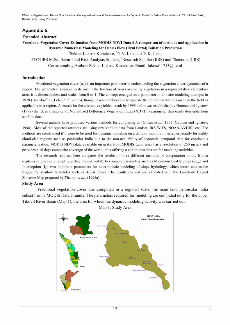
Effect of Vegetation on Debris Flow Initiation - Conceptualisation and Parameterisation of a Dynamic Model for Debris Flow Initiation in Tikovil River Basin, Kerala, India, using PCRaster
117
Appendix 5: Extended Abstract Fractional Vegetation Cover Estimation from MODIS NDVI Data ñ A comparison of methods and application in
Dynamic Numerical Modeling for Debris Flow (Urul Pottal) Initiation Prediction 1Sekhar Lukose Kuriakose, 2N.V. Lele and 3P.K. Joshi
1ITC/IIRS M.Sc. Hazard and Risk Analysis Student, 2Research Scholar (IIRS) and 3Scientist (IIRS) Corresponding Author: Sekhar Lukose Kuriakose. Email: [email protected]
Introduction
Fractional vegetation cover (σv) is an important parameter in understanding the vegetation cover dynamics of a region. The parameter is simple in its own ñ the fraction of area covered by vegetation in a representative elementary area; it is dimensionless and scales from 0 to 1. The concept emerged as a parameter in climatic modeling attempts in 1978 (Deardorff in (Lele et al., 2005)), though it was cumbersome to upscale the point observations made in the field as applicable to a region. A search for the alternative yielded result by 1998 and it was established by Gutman and Ignatov (1998) that σv is a function of Normalized Difference Vegetation Index (NDVI), a parameter thus easily derivable from satellite data.
Several authors have proposed various methods for computing σv (Gillies et al., 1997; Gutman and Ignatov, 1998). Most of the reported attempts are using raw satellite data from Landsat, IRS WiFS, NOAA/AVHRR etc. The methods are constrained if it were to be used for dynamic modeling on a daily or monthly timestep especially for highly cloud-clad regions such as peninsular India due to the non-availability of sequential temporal data for continuous parameterization. MODIS NDVI data available on gratis from MODIS Land team has a resolution of 250 meters and provides a 16 days composite coverage of the world, thus offering a continuous data set for modeling activities.
The research reported here compares the results of three different methods of computation of σv. It also explains in brief an attempt to utilize the derived σv to compute parameters such as Maximum Leaf Storage (Smax) and Interception (Ic), two important parameters for deterministic modeling of slope hydrology, which inturn acts as the trigger for shallow landslides such as debris flows. The results derived are validated with the Landslide Hazard Zonation Map prepared by Thampi et al., (1998a). Study Area
Fractional vegetation cover was computed in a regional scale; the main land peninsular India subset from a MODIS Data Granule. The parameters required for modeling are computed only for the upper Tikovil River Basin (Map 1), the area for which the dynamic modeling activity was carried out.
Map 1: Study Area

Effect of Vegetation on Debris Flow Initiation - Conceptualisation and Parameterisation of a Dynamic Model for Debris Flow Initiation in Tikovil River Basin, Kerala, India, using PCRaster
118
Materials and Methods The conventional method of deriving σv is with the equation:
Equation 1 where, NDVImax the Maximum NDVI value in a given image, NDVImin the minimum NDVI value
in a given image and NDVIi the image itself. Gutman and Ignatov (1998) suggested an improvement to this method by using the NDVI value for the purest vegetation pixel as NDVImax and the NDVI value for the purest baresoil pixel as the NDVImin. Walthall et al., (2004) reported a further revision to the method by making it more sensitive to actual vegetation cover on ground. They suggested the equation:
Equation 2 where, NDVImax the maximum non spurious NDVI value in a given image, NDVImin the minimum
non spurious NDVI value in a given image, NDVIi the image itself and kc the crop factor of the respective vegetation cover on ground. Standard values of kc derived from FAO database can be used for the purpose.
Non-spurious NDVI values were derived using the approach recommended by Gutman and Ignatov (1998). The later approach was adopted here given the availability of pure soil and vegetation pixel locations from previous research works and by identifying them from the FCC created for February composite bands originally used by the Land Team to compute the NDVI data, available along side the NDVI data. Average values of as many as 56 true vegetation pixels and 62 true soil pixels were used as the NDVImax and NDVImin values, respectively. The computation of σv for the area of interest for modeling was carried out using the average kc value of all the major vegetation types seen in the area.
The σv computed was used to compute Leaf Area Index (-) as suggested by Walthall et al., (2004); the equation for which is:
Equation 3 where, fc is σv. LAI is related to Maximum Canopy Storage (mm/pixel) by Von Hoyningen-Huene (1981) as:
Equation 4 σv, and Smax are used to compute Interception, S (mm/pixel/day), using the equation suggested by Aston (1979), which is:
Equation 5 where, Cp is σv, Pcum is cumulated rainfall and k a correction factor for vegetation density [(-),
(equals 0.046*LAI)]. Results and Discussion The methods were applied on the composite NDVI data sets of 2001 for the months of June to December. Computed σv shows that the conventional method estimates the parameter on the extreme side, given the bias due to spurious pixels. Gutman and Igantov method as well indicates a trend nearer to that of conventional. However σv computed using Walthall et al. (2004) method with two different kc values (0.2 and 0.8) shows that the method is highly sensitive to the crop factors (Graph 1). The method thus extends

Effect of Vegetation on Debris Flow Initiation - Conceptualisation and Parameterisation of a Dynamic Model for Debris Flow Initiation in Tikovil River Basin, Kerala, India, using PCRaster
119
the capability of σv as a parameter directly sensitive to the actual vegetation types on the ground and so can be inferred more reliable than the other two.
Given this inference the method was adopted to compute the σv for the area of interest for modeling and the kc value of 0.6 was used. The resultant images were used to compute the subsequent parameters. By providing the cumulative rainfall on a daily timestep (considering the interim dry days, which means cumulation stops when there is a dry day in between), the daily interception values for the seven months were derived (Map 2). Maximum Canopy Storage is the maximum amount of precipitation that can be held in the leaves and was computed for every month.
The resultant daily and monthly time series maps were input into the coupled model STARWARS + PROBSTAB (Storage and Redistribution of Water on Agricultural and Revegetated Slopes + Probability of Stability) (van Beek, 2002), which enables the prediction of transient hydrological conditions that results in shallow landsliding. The model results were validated using the Landslide Hazard Zonation map for the study area prepared by Thampi et al., (1998a) by visibly comparing the area marked critical in the map with the Probability of Failure Map derived from the model.
FRACTIONAL VEGETATION COVER FOR SOIL PIXELS
0
0.05
0.1
0.15
0.2
0.25
1 2 3 4 5 6 7
Gutman Walthall (0.2) Walthall (0.8) Conventional
FRACTIONAL VEGETATION COVER FOR VEGETATION PIXELS
0.00
0.20
0.40
0.60
0.80
1.00
1 2 3 4 5 6 7
Gutman Conventional Walthall (0.2) Walthall (0.8)
Graph 1 ñ Comparison of σv computed from different methods
Map 1: Interception Maps Prepared from MODIS computed σv

Effect of Vegetation on Debris Flow Initiation - Conceptualisation and Parameterisation of a Dynamic Model for Debris Flow Initiation in Tikovil River Basin, Kerala, India, using PCRaster
120
Conclusion The research clearly concludes that σv computed using Walthall et al., (2004) method is highly sensitive to actual vegetation cover of a given area. The method if coupled and used with a well-prepared landuse map can provide landuse specific σv values and thus make the process more site specific. σv is a parameter that has multifarious applications (Lele et al., 2005). In conditions were field data is deficient for numerical modeling, satellite data based parameterization is the most economic and thus needs to be further researched. Readily available data sets such as, MODIS NDVI are a solace for scientists as they expedite the overall process of rigorous data demanding mathematical modelling attempts.

Effect of Vegetation on Debris Flow Initiation - Conceptualisation and Parameterisation of a Dynamic Model for Debris Flow Initiation in Tikovil River Basin, Kerala, India, using PCRaster
121
Authorís Resume
Contact Address: Sekhar L.K, T.C 12/1242, Attara Lane, Kannanmoola, Medical College P.O,
Trivandrum, Kerala, India ñ 695 011 Email: [email protected], [email protected] Telephone: (Res) - +91 (0) 471-2551803 Summary of Career The author completed his M.Sc in Applied Geography from University of Madras in the year 2001. From then on till 2003 he worked as Consultant (GIS) for Parambikulam Wildlife Sanctuary, Kerala Forests and Wildlife Department in creating a customized GIS and preparing a 10 year management plan of the sanctuary. He was also Consultant (GIS) to Enter Technologies Pvt. Ltd, Technopark, Trivandrum, during the same period. Later on, he took on the position of Management Plan and GIS Specialist of Gulf of Mannar Marine National Park and served the office till June 2004 after which he joined the M.Sc GIS and EOS for Natural Hazards and Risk Analysis jointly offered by ITC and IIRS. There are 8 papers, a multimedia CDRom published by Kerala Forests and Widlife Department and two websites as publications in his credit. His research interests are:
• Modeling of vegetation effects on landscape evolution • Remote Sensing and GIS for Natural Disaster Management • GIS Implementation and Customization for Forestry Applications • Computer Applications for Indigenous People Management and Development • Geographical Thought