Embed Size (px)
Citation preview

2040 Sheridan Rd. Evanston, IL 60208-4100 Tel: 847-491-3395 Fax: 847-491-9916 www.northwestern.edu/ipr, [email protected]
Institute for Policy Research Northwestern University Working Paper Series
WP-07-13
Effect Sizes in Three Level Cluster Randomized Experiments
Larry V. Hedges Faculty Fellow, Institute for Policy Research
Board of Trustees Professor of Statistics and Social Policy Northwestern University
DRAFT Please do not quote or distribute without permission.

Abstract
Research designs involving cluster randomization are becoming increasingly important in
educational and behavioral research. Many of these designs involve two levels of
clustering or nesting (students within classes and classes within schools). Researchers
would like to compute effect size indexes based on the standardized mean difference to
compare the results of cluster randomized studies with other studies and to combine
information across studies in meta-analyses. This paper addresses the problem of
defining effect sizes in designs with two levels of clustering and computing estimates of
those effect sizes and their standard errors from information that is likely to be reported
in journal articles. Five effect sizes are defined corresponding to different
standardizations. Estimators of each effect size index are also presented along with their
sampling distributions (including standard errors).

Effect Sizes in Three Level Experiments 3
Effect Sizes in Three Level Cluster Randomized Experiments
Educational experiments or quasi-experiments used to evaluate the effects of educational interventions, products or technologies often involve several sites (typically schools). One common design assigns entire schools to the same treatment group, with different schools assigned to different treatments. This design is often called a cluster randomized design because schools correspond to statistical clusters. Several analysis strategies for cluster randomized trials such as this are possible, including analyses of variance using clusters as a nested factor (see, e.g., Hopkins, 1982) and analyses involving hierarchical linear models (see e.g., Raudenbush and Bryk, 2002). For general discussions of the design and analyses of cluster randomized experiments see Raudenbush and Bryk (2002), Donner and Klar (2000), Klar and Donner (2001), Murray (1998), or Murray, Varnell, & Blitstein (2004).
Problems of representation of the results of cluster randomized trials (and the corresponding quasi-experiments) in the form of effect sizes and combining them across studies in meta-analyses have received less attention. Rooney and Murray (1996) called attention to the problem of effect size estimation for meta-analysis involving cluster randomized trials. They suggested that conventional estimates were not appropriate and noted that formulas for standard errors that assumed simple random sampling (rather than clustered sampling) were incorrect. Donner and Klar (2002) suggested that corrections for the effects of clustering should be introduced in meta-analyses of cluster randomized experiments. Hedges (in press) suggested definitions of several effect size parameters in cluster randomized experiments with one level of clustering or nesting (so called two-level designs) and gave their sampling distributions. Each of these papers cited above examined meta-analysis for studies using only one level of clustering (that is, two level designs).
The admittedly limited work on the effects of clustering on estimates of effect size and their combination in meta-analysis appears to have had little impact on the practice of meta-analysis. Laopaiboon (2003) reviewed the methods used in 25 published meta-analyses involving cluster randomized experiments, and found that only 3 used methods to account for clustering in their analysis. All of these three were meta-analyses of health care studies using binary outcomes. Of the six meta-analyses involving education, none used methods that addressed the impact of clustering.
The work reported in this paper was stimulated by problems faced by the US Department of Education’s What Works Clearinghouse, whose mission is to evaluate, compare, and synthesize evidence of effectiveness of educational programs, products, practices, and policies. The What Works Clearinghouse reviewers found that the majority of the high quality studies they were examining involved assignment of treatment by schools, which led to clustering that needed to be taken into account in computing an estimate of effect size and its uncertainty. While some of these studies involved only one classroom per school, others involved multiple classrooms per school and thus the studies have three level designs involving a second level of clustering that may need to be taken into account.
While methods have now been developed for computing effect size estimates and their sampling properties in two level designs (e.g., Hedges, in press), less is known about methods for taking into account the two levels of clustering that are present in three
Effect Sizes in Three Level Experiments 4
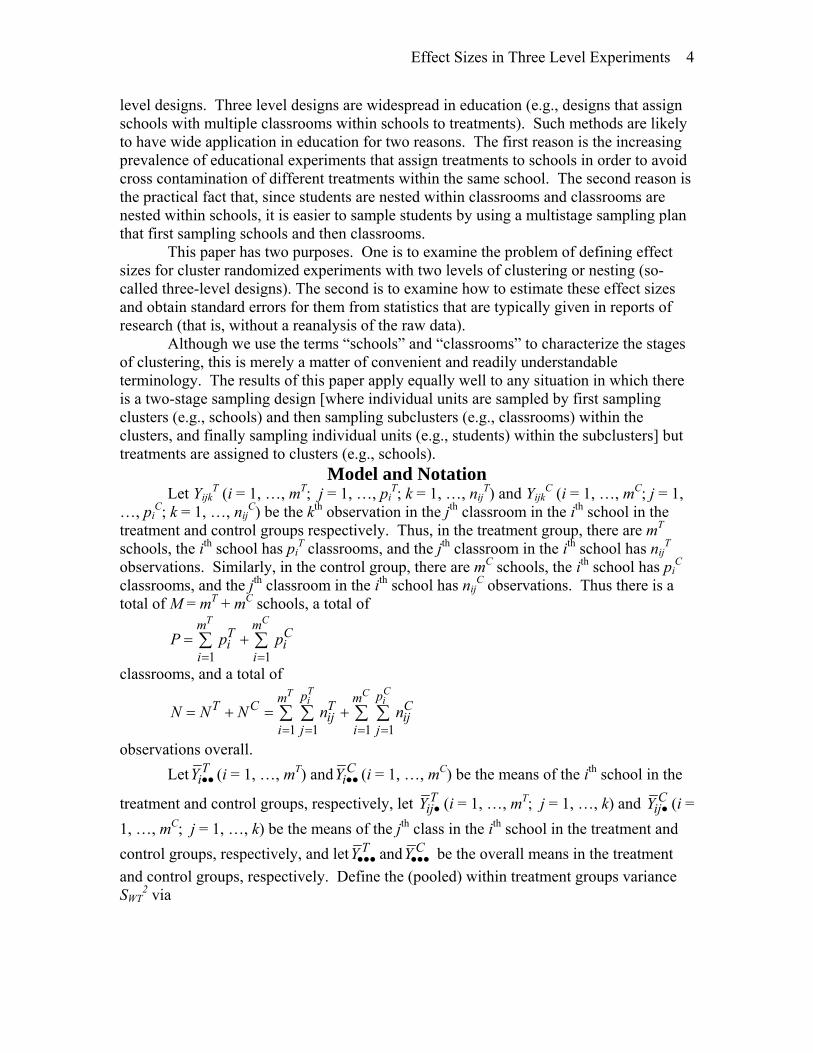
level designs. Three level designs are widespread in education (e.g., designs that assign schools with multiple classrooms within schools to treatments). Such methods are likely to have wide application in education for two reasons. The first reason is the increasing prevalence of educational experiments that assign treatments to schools in order to avoid cross contamination of different treatments within the same school. The second reason is the practical fact that, since students are nested within classrooms and classrooms are nested within schools, it is easier to sample students by using a multistage sampling plan that first sampling schools and then classrooms.
This paper has two purposes. One is to examine the problem of defining effect sizes for cluster randomized experiments with two levels of clustering or nesting (so-called three-level designs). The second is to examine how to estimate these effect sizes and obtain standard errors for them from statistics that are typically given in reports of research (that is, without a reanalysis of the raw data).
Although we use the terms “schools” and “classrooms” to characterize the stages of clustering, this is merely a matter of convenient and readily understandable terminology. The results of this paper apply equally well to any situation in which there is a two-stage sampling design [where individual units are sampled by first sampling clusters (e.g., schools) and then sampling subclusters (e.g., classrooms) within the clusters, and finally sampling individual units (e.g., students) within the subclusters] but treatments are assigned to clusters (e.g., schools).
Model and Notation Let Yijk
T (i = 1, …, mT; j = 1, …, piT; k = 1, …, nij
T) and YijkC (i = 1, …, mC; j = 1,
…, piC; k = 1, …, nij
C) be the kth observation in the jth classroom in the ith school in the treatment and control groups respectively. Thus, in the treatment group, there are mT schools, the ith school has pi
T classrooms, and the jth classroom in the ith school has nijT
observations. Similarly, in the control group, there are mC schools, the ith school has piC
classrooms, and the jth classroom in the ith school has nijC observations. Thus there is a
total of M = mT + mC schools, a total of
1 1
T Cm mT Ci i
i iP p p
= == +∑ ∑
classrooms, and a total of
1 1 1 1
T CT Ci ip pm mT C T
ij iji j i j
N N N n n= = = =
= + = +∑ ∑ ∑ ∑ C
observations overall. Let T
iY •• (i = 1, …, mT) and CiY •• (i = 1, …, mC) be the means of the ith school in the
treatment and control groups, respectively, let TijY • (i = 1, …, mT; j = 1, …, k) and C
ijY • (i = 1, …, mC; j = 1, …, k) be the means of the jth class in the ith school in the treatment and control groups, respectively, and let TY••• and CY••• be the overall means in the treatment and control groups, respectively. Define the (pooled) within treatment groups variance SWT
2 via

Effect Sizes in Three Level Experiments 5
2 2
1 1 1 1 1 12( ) ( )
2
T CT CT Cij iji in np pm mT T C Cijk ijk
i j k i j kWT
Y Y Y YS
N
••• •••= = = = = =
− + −
=−
∑ ∑ ∑ ∑ ∑ ∑, (1)
the pooled within-schools variance SWS2 via
2 2
1 1 1 1 1 12( ) ( )
T CT CT Cij iji in np pm mT T C Cijk i ijk i
i j k i j kWS
Y Y Y YS
N M
•• •= = = = = =
− + −
=−
∑ ∑ ∑ ∑ ∑ ∑ •
, (2)
and the (pooled) within-classroom sample variance SWC2 via
2 2
1 1 1 1 1 12( ) ( )
T CT CT Cij iji in np pm mT T C Cijk ij ijk ij
i j k i j kWC
Y Y Y YS
N P
• •= = = = = =
− + −
=−
∑ ∑ ∑ ∑ ∑ ∑. (3)
Define the between schools but within treatment groups variance SBS2 via
2 2
1 122
T Cm mT T C Ci i
j jBS
(Y Y ) (Y Y )S
M
•• ••• •• •••= =
− + −
=−
∑ ∑, (4)
and the (pooled) between classrooms but within treatment groups and schools variance SBC
2 via
2 2
1 1 1 12( ) ( )
T CT Ci ip pm mT T C C
ij i ij ii j i j
BC
Y Y Y YS
P M
• •• • ••= = = =
− + −
=−
∑ ∑ ∑ ∑. (5)
Suppose that observations within the jth classroom in the ith school within the treatment and control group groups are normally distributed about classroom means μij
T and μij
C with a common within-cluster variance σWC2. That is
2( ,T Tijk ij WCY N μ σ )
)
)
)
)BS
, i =1, …, mT; j = 1, …, piT; k = 1, …, nij
T
and 2( ,C C
ijk ij WCY N μ σ , i =1, …, mC; j = 1, …, piC; k = 1, …, nij
C. Suppose further that the classroom means are random effects (for example they are considered a sample from a population of means) so that the class means themselves have a normal distribution about the school means μi●
T and μi●C and common variance σBC
2. That is
2( ,T Tij i BCμ N μ σ• , i = 1, …, mT; j = 1, ..., pi
T
and 2( ,C C
ij i BCμ N μ σ• , i = 1, …, mC; j = 1, ..., piC.
Finally suppose that the school means μi●T and μi●
C are also normally distributed about the treatment and control group means μ●●T and μ●●C with common variance σBS
2. That is 2( ,T T
iμ N μ σ• •• , i = 1, …, mT
and
Effect Sizes in Three Level Experiments 6
2( ,C Ciμ N μ σ• •• )BS , i = 1, …, mC.
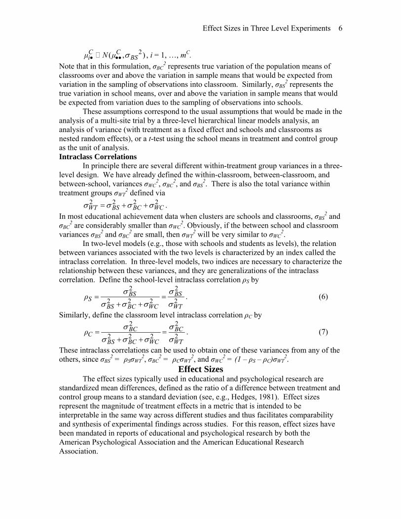
Note that in this formulation, σBC2 represents true variation of the population means of
classrooms over and above the variation in sample means that would be expected from variation in the sampling of observations into classroom. Similarly, σBS
2 represents the true variation in school means, over and above the variation in sample means that would be expected from variation dues to the sampling of observations into schools.
These assumptions correspond to the usual assumptions that would be made in the analysis of a multi-site trial by a three-level hierarchical linear models analysis, an analysis of variance (with treatment as a fixed effect and schools and classrooms as nested random effects), or a t-test using the school means in treatment and control group as the unit of analysis. Intraclass Correlations In principle there are several different within-treatment group variances in a three-level design. We have already defined the within-classroom, between-classroom, and between-school, variances σWC
2, σBC2, and σBS
2. There is also the total variance within treatment groups σWT
2 defined via . 2 2 2 2
WT BS BC WCσ σ σ σ= + +In most educational achievement data when clusters are schools and classrooms, σBS
2 and σBC
2 are considerably smaller than σWC2. Obviously, if the between school and classroom
variances σBS2 and σBC
2 are small, then σWT2 will be very similar to σWC
2. In two-level models (e.g., those with schools and students as levels), the relation between variances associated with the two levels is characterized by an index called the intraclass correlation. In three-level models, two indices are necessary to characterize the relationship between these variances, and they are generalizations of the intraclass correlation. Define the school-level intraclass correlation ρS by
2 2
2 2 2 2BS BS
SBS BC WC WT
ρ σ σσ σ σ σ
=+ +
= . (6)
Similarly, define the classroom level intraclass correlation ρC by
2 2
2 2 2 2BC BC
CBS BC WC WT
ρ σ σσ σ σ σ
=+ +
= . (7)
These intraclass correlations can be used to obtain one of these variances from any of the others, since σBS
2 = ρSσWT2, σBC
2 = ρCσWT2, and σWC
2 = (1 – ρS – ρC)σWT2.
Effect Sizes The effect sizes typically used in educational and psychological research are
standardized mean differences, defined as the ratio of a difference between treatment and control group means to a standard deviation (see, e.g., Hedges, 1981). Effect sizes represent the magnitude of treatment effects in a metric that is intended to be interpretable in the same way across different studies and thus facilitates comparability and synthesis of experimental findings across studies. For this reason, effect sizes have been mandated in reports of educational and psychological research by both the American Psychological Association and the American Educational Research Association.

Effect Sizes in Three Level Experiments 7
In single level designs the notion of standardized mean difference is often unambiguous: There is only one possibility because there is only one within-treatment-groups standard deviation. In multi-site designs and multi-level designs such as cluster randomized trials, there are several possible standardized mean differences. The possibilities in two level designs were discussed by Hedges (in press). In this section we clarify the possible effect size definitions in three-level designs.
The alternative possibilities for the standard deviation lead to different possible definitions for the population effect size in three-level designs. The choice of one of these effect sizes should be determined on the basis of the inference of interest to the researcher. If the effect size measures are to be used in meta-analysis, an important inference goal may be to estimate parameters that are comparable with those that can be estimated in other studies. In such cases, the standard deviation may be chosen to be the same kind of standard deviation used in other studies to which this study will be compared. We focus on three effect sizes that seem likely to be the most useful (meaning the most widely used), but indicate two others that may be useful in some circumstances. One effect size standardizes the mean difference by the total standard deviation within-treatment groups. It is of the form
T C
WTWT
μ μδσ•• ••−
= . (8)
The effect size δWT might be of interest in a meta-analysis where the other studies have three-level designs involving multiple schools and classrooms or studies that sample from a broader population but do not include schools or classes as clusters in the sampling design (this would typically imply that they used an individual, rather than a cluster, assignment strategy). In such cases, δWT might be the effect size that is most comparable with the effect sizes in other studies. If σBC
2 + σWC2 ≠ 0 (and hence ρS ≠ 1), a second effect size can be defined that
standardizes the mean difference by the standard deviation within-schools. It is of the form
2 2 1
T CWT
WSSBC WC
δμ μδρ
•• ••−= =
−+σ σ. (9)
The effect size δWS might be of interest in a situation where most of the studies of interest had two level designs involving multiple schools. In such studies δWS may (implicitly or explicitly) be the effect size estimated and hence be most comparable with the effect size estimates of the other studies. If σWC ≠ 0 (and hence ρS + ρC ≠ 1), a third effect size can be defined that standardizes the mean difference by the within-classroom standard deviation. It has the form
1
1 1
T CWS SWT
WCWC S C S C
δ ρδμ μδρ ρ ρ
•• •• −−= = =
− − − −σ ρ. (10)
The effect size δWC might be of interest, for example, in a meta-analysis where the other studies to which the current study is compared are typically studies with a single school. In such studies δWC may (implicitly) be the effect size estimated and hence δWC might be the effect size most comparable with the effect size estimates in other studies.

Effect Sizes in Three Level Experiments 8
Two other effect sizes that standardize the mean difference by between classroom and between school standard deviations may be of interest (although less frequently). If σBS ≠ 0 (and hence ρS ≠ 0), a fourth possible effect size would be
T C
WTBS
BS S
δμ μδρ
•• ••−= =
σ. (11)
The effect size δBS may also be of interest in a meta-analysis where the studies being compared are typically multi-level studies that have been analyzed by using school means as the unit of analysis. This effect size is less likely to be of general interest, but it might be of interest in cases where the outcome variable on which the treatment effect is defined is conceptually at the level of schools and the individual observations are of interest only because the average defines an aggregate property.
For example, Bryk and Schneider (2000) study the level of school trust as an important predictor of school functioning. Trust level in a school is measured as an aggregate of reported trust scores of individual students or teachers, but only the school means are meaningful as measures of trust as a property of the school. Thus an intervention that was targeted at increasing school trust might well measure trust in a school as the mean of trust scores across students, and evaluate the treatment effect as the difference in means between all students in schools assigned to the treatment group and those in schools assigned to the control group. In this case, only σBS represents a standard deviation of a meaningful aggregate (school average trust), while σBC and σWC do not, and therefore only δBS seems conceptually meaningful as an effect size.
If σBC ≠ 0 (and hence ρC ≠ 0), a fifth possible effect size would be
T C
WTBC
BC C
δμ μδρ
•• ••−= =
σ. (12)
The effect size δBC may also be of interest in a meta-analysis where the studies being compared are typically multi-level studies that have been analyzed by using classroom means as the unit of analysis or the outcome is conceptually defined as a classroom-level property. This effect size might be of interest in cases where the outcome variable on which the treatment effect is defined conceptually at the level of classrooms and the individual observations are of interest only because the classroom average defines an aggregate property.
For example, consider classroom climate as an important determinant of instructional effectiveness (see, e.g., Dunkin and Biddle, 1974). Classroom climate is measured as an aggregate of reports by students, but only classroom means are meaningful as measures of classroom climate. An intervention that was intended to improve classroom climate might well measure the intervention effect via the difference between the means of classrooms assigned to the intervention group and those assigned to the control group. In this case both σBC and σBS represent standard deviations of a meaningful aggregate score (while σWC does not). Therefore either δBS or δBC would be conceptually meaningful effect sizes, but δBC might be preferred if many studies were carried out within single schools.
Because ρS and ρC will often be rather small, δWS and δWC will often be similar in magnitude to δWT. For the same reason, δBS and δBC will typically be much larger (in the same population) than δWS, δWC, or δWT. Note also that if all of the effect sizes are defined (that is, if 0 < ρS < 1, 0 < ρC < 1, and ρS + ρC < 1), any one of these effect sizes may be

Effect Sizes in Three Level Experiments 9
obtained algebraically from any of the others, provided ρC and ρS are known. In particular, equations (8) through (11) can be solved for δWT in terms of any of the other effect sizes, ρS, and ρC. These same equations, in turn can be used to define any of the five effect sizes in terms of δWT.
Estimates of Effect Sizes: Equal Sample Sizes In this section we present estimates of the effect sizes and their approximate sampling distributions when all of the schools have the same number, p, of classrooms, that is when pi
T = p, i = 1, …, mT and piC = p, i = 1, …, mC , and all the classroom sample
sizes are equal to n, that is when nijT = n, i = 1, …, mT; j = 1, …, p and nij
C = n, i = 1, …, mC; j = 1, …, p In this case NT = npmT , NC = npmC , and N = NT + NC = np(mT + mC) = nM. Derivations and the details of the small sample distribution of the effect size estimators are given in the Appendix.
We present results explicitly for the case of equal school and classroom sample sizes for two reasons. The first reason is that most designs attempt to achieve equal sample sizes but specific (realized) school and classroom sample sizes are rarely reported, so that the equal sample size formulas will be of most practical use. The second reason is that the results become considerably more complicated when sample sizes are unequal—sufficiently complicated that it is difficult to obtain much insight from examining the formulas in the unequal sample size case. Estimation of δWC
We start with estimation of δWC, which is the most straightforward. If ρS + ρC ≠ 1, then δWC is defined and the estimate
T C
WCWC
Y YdS
••• •••−= (13)
is a consistent estimator of δWC. The estimator dWC is approximately normally distributed about δWC with variance
21 ( 1) ( 1){ }
(1 ) 2( )S C WC
WCS C
pn ρ n ρ δV dmpn ρ ρ N Mp
+ − + −= +
− − −%, (14)
where
T C
T Cm mm
m m=
+% .
An estimate vWC of the variance of dWC can be computed by substituting the consistent estimate dWC for δWC in equation (14) above. The leading term of the variance in equation (14) arises from uncertainty in the mean difference. Note that it is [1 + (pn – 1)ρS + (n – 1)ρC]/(1 – ρS – ρC)] as large as would be expected if there were no clustering in the sample (that is if ρS = ρC = 0). Thus [1 + (pn – 1)ρS + (n – 1)ρC]/(1 – ρS – ρC)] is a kind of variance inflation factor for the variance of the effect size estimate dWC. Note that if either ρS = 0 or ρC = 0, there is no clustering at one level and the three-level design logically reduces to a two-level design. If ρS = 0, the expression (13) for dWC and expression (14) for its variance reduce to those given in equations (7) and (8) in Hedges (in press) for the corresponding effect size estimate (called there dW) and its variance in a two-level design with clusters of size n and intraclass correlation ρ = ρC. Similarly, if ρC = 0, expressions (13) and (14) reduce to the estimate given in equation (7)

Effect Sizes in Three Level Experiments 10
and its variance given in equation (8) of Hedges (in press) with cluster size np and intraclass correlation ρ = ρS. If ρS = ρC = 0 so that there is no clustering by classroom or by school, the design is logically equivalent to a one-level design. In this case the expression (13) for dWC and expression (14) for its variance reduce to the usual expressions for the standardized mean difference and its variance (see, e.g., Hedges, 1981). Estimation of δWS
If ρS ≠ 1,then δWS is defined and an estimate of δWS can also be obtained from the mean difference and SWS if the intraclass correlations ρS and ρC are known or can be imputed. A direct argument shows that a consistent estimator of δWS is
( )( )( )
11 1
1T C
CWS
WS S
n ρY YdS ρ np
••• •••⎛ ⎞ −−= −⎜ ⎟⎜ ⎟ − −⎝ ⎠
. (15)
The estimate dWS is normally distributed in large samples with variance
{ } ( )
( ) ( ) ( )
2
22
1 ( 1) ( 1)1
( 1) 2 1 1
2 1 1 1 ( 1) (1
S CWS
S
2 22 C CWS
S C
pn ρ n ρV dmpn ρ
pn ρ n( p )ρρ n ( p )ρδM pn ρ pn n ρ ρ
+ − + −=
−
⎛ ⎞⎜ ⎟− + − + −
+ ⎜ ⎟⎡ ⎤− − − − − −⎜ ⎟⎢ ⎥⎣ ⎦⎝ ⎠
%
)S
, (16)
where ρ = (1 – ρS – ρC). An estimate vWS of the variance of dWS can be computed by substituting the consistent estimate dWS for δWS in equation (16) above. The leading term of the variance in equation (16) arises from uncertainty in the mean difference. Note that it is [1 + (pn – 1)ρS + (n – 1)ρC]/(1 – ρS)] as large as would be expected if there were no clustering in the sample (that is if ρS = ρC = 0). Thus the term [1 + (pn – 1)ρS + (n – 1)ρC]/(1 – ρS )] is a kind of variance inflation factor for the variance of the effect size estimate dWS. Note that if ρC = 0 so that there is no clustering effect by classrooms, the three level design is logically equivalent to a two-level design. In this case, the expression (15) for dWS and expression (16) for its variance reduce to those given in equations (7) and (8) in Hedges (in press) for the corresponding effect size estimate (called there dW) and its variance in a two-level design with clusters of size pn and intraclass correlation ρ = ρS. If ρS = ρC = 0 so that there is no clustering by classroom or by school, the design is logically equivalent to a one-level design. In this case the expression (15) for dWS and expression (16) for its variance reduce to those for the standardized mean difference and its variance in a one-level design (see, e.g., Hedges, 1981). Estimation of δWT
An estimate of δWT can also be obtained from the mean difference and SWT if the intraclass correlations ρS and ρC are known or can be imputed. A direct argument shows that a consistent estimator of δWT is
2( 1) 2( 1)12
T CS
WTWT
pn ρ nY YdS N
Cρ••• •••⎛ ⎞ − + −−= −⎜ ⎟⎜ ⎟ −⎝ ⎠
. (17)
The estimate dWT is normally distributed in large samples with variance

Effect Sizes in Three Level Experiments 11
{ }
[ ]2 2 2
S C
1 ( 1) ( 1)
( 2) 2 22( 2) ( 2) 2( 1) 2( 1)
S CWT
2 S C S C S CWT
pn ρ n ρV dmpn
pnNρ nNρ N ρ nNρ ρ Nρ ρ+2Nρ ρδN N pn ρ n ρ
+ − + −=
⎛ ⎞+ + − + ++ ⎜ ⎟⎜ ⎟− − − − − −⎝ ⎠
%) ( ) ) ( , (18)
where N)
= (N – 2pn), = (N – 2n), andN(
ρ = 1 – ρS – ρC. An estimate vWT of the variance of dWT can be computed by substituting the consistent estimate dWT for δWT in equation (18) above. The leading term of the variance in equation (18) arises from uncertainty in the mean difference. Note that this leading term is [1 + (np – 1)ρS + (n – 1)ρC] as large as would be expected if there were no clustering in the sample (that is if ρS = ρC = 0). The term [1 + (np – 1)ρS + (n – 1)ρC] is a generalization to two stages of clustering of the variance inflation factor mentioned by Donner (1981) for the variance of means in clustered samples (with one stage of clustering) and also corresponds to a variance inflation factor for the effect size estimate dWT. Note that if ρC = 0 so that there is no clustering by classrooms, or if ρS = 0 so that there is no clustering by schools, the three-level design is logically equivalent to a two-level design. If ρS = 0, the expression (17) for dWT and expression (18) for its variance reduce to those given in equations (15) and (16) in Hedges (in press) for the corresponding effect size estimate and its variance in a two-level design with clusters of size n and intraclass correlation ρ = ρC. Similarly, if ρC = 0, expressions (17) and (18) reduce to the estimate given in equation (15) and its variance given in equation (16) of Hedges (in press) for the corresponding effect size in a two-level design with cluster size np and intraclass correlation ρ = ρS. Estimation of δBC
If ρC ≠ 0 (so that δBC is defined), SBC may be used, along with the intraclass correlations ρS and ρC, to obtain an estimate of δBC. A direct argument shows that
1 ( 1)T CS
BCBC C
Cρ n ρY YdS nρ
••• ••• − + −−= (19)
is a consistent estimate of δBC. This estimate is normally distributed in large samples with variance
21 ( 1) [1 ( 1) ]{ }
2 ( 1)S C S C
BCC C
BCρ n ρ ρ + n ρ δV dmpnρ M p nρ
− + − − −= +
−%. (20)
An estimate vBC of the variance of dBC can be computed by substituting the consistent estimate dBC for δBC in equation (20) above. Note that the presence of ρC in the denominator of the estimator and its variance is possible since the effect size parameter only exists if ρC ≠ 0. The variance in equation (20) is [1 – ρS + (n – 1)ρC]/nρC] as large as the variance of the standardized mean difference computed from an analysis using class means as the unit of analysis if the data had come from a simple random sample. Thus [1 – ρS + (n – 1)ρC]/nρC] is a kind of variance inflation factor for the variance of effect size estimates like dBC compared to this alternative effect size estimate. Note that if ρS = 0 so that there is no clustering by school, the expression (19) for dBC and expression (20) for its variance reduce to those given in equations (11) and (12)

Effect Sizes in Three Level Experiments 12
in Hedges (in press) for the corresponding effect size estimate (called there dB2) and its variance in a two-level design with clusters of size n and intraclass correlation ρ = ρC. Estimation of δBS
If ρS ≠ 0 (so that δBS is defined), SBS may be used, along with the intraclass correlations ρS and ρC, to obtain an estimate of δBS. A direct argument shows that
1 ( 1) ( 1)T CS
BSBS S
pn Cρ n ρY YdS pnρ
••• ••• − − + −−= (21)
is a consistent estimate of δBS. This estimate is normally distributed in large samples with variance
21 ( 1) ( 1) [1+( 1) ( 1) ]{ }
2( 2)S C S C
BSS S
pn BSρ n ρ pn ρ + n ρ δV dmpnρ M pnρ
+ − + − − −= +
−%. (22)
An estimate vBS of the variance of dBS can be computed by substituting the consistent estimate dBS for δBS in equation (22) above. Note that the presence of ρS in the denominator of the estimator and its variance is possible since the effect size parameter only exists if ρS ≠ 0. The variance in equation (22) is [1 + (pn – 1)ρS + (n – 1)ρC]/pnρS] as large as the variance of the standardized mean difference computed from a simple random sample. Thus [1 – ρS + (n – 1)ρC]/pnρS] is a kind of variance inflation factor for the variance of effect size estimates like dBS compared to this alternative effect size estimate. Note that if ρC = 0 so that there is no clustering by classroom, expressions (21) and (22) reduce to the corresponding effect size estimate (called there dB2) given in equation (11) and its variance given in equation (12) of Hedges (in press) in a two-level design with cluster size np and intraclass correlation ρ = ρS.
Estimation of Effect Size: Unequal Sample Sizes When classroom or school sample sizes are unequal, expressions for the effect size estimates are more complex and expressions for their variances are much more complex. In this section we give expressions for several of the effect size estimates and their sampling distributions. These expressions may be of use in cases where the number of classrooms and students within classrooms are markedly unequal and they are given explicitly in reports of research. They also provide some in sight into what single “compromise” value of p and n might give most accurate results when substituted in to equal sample size formulas. Estimation of δWC
If ρS + ρC ≠ 1, then the estimate dWC of δWC when sample sizes are unequal is identical to that in the equal sample size case given in equation (13), and it is approximately normally distributed. However in the case of unequal sample sizes, the variance is given by
21 ( 1) ( 1){ }
(1 ) 2( )U S U C WC
WCS C
p ρ n ρ δV dN ρ ρ N P
+ − + −=
− − −%+ , (23)
where

Effect Sizes in Three Level Experiments 13
2 2
1 1 1 1
T CT Ci ip pm mC T T C
ij iji j i j
U T
N n N n
pNN NN
= = = =
⎛ ⎞ ⎛⎜ ⎟ ⎜⎜ ⎟ ⎜⎝ ⎠ ⎝= +
∑ ∑ ∑ ∑
C
⎞⎟⎟⎠ , (24)
( ) ( )2 2
1 1 1 1
T CT Ci ip pm mC T T C
ij iji j i j
U T
N n N nn
NN NN= = = == +∑ ∑ ∑ ∑
C , (25)
T C
TN NN
N N=
+%
C ,
and
1 1
T Cm mT Ci i
i iP p p
= == +∑ ∑
is the total number of classrooms. Note that if if all the niT and ni
C are equal to n, then nU = n, and that if all the pi
T and piC are equal to p, then pU = pn, and P = Mp, so that (23)
reduces to (14). As in the case of the equal sample size formulas an estimate vWC of the variance of dWC can be computed by substituting the consistent estimate dWC for δWC in equation (23) above. Estimation of δWS
If ρS ≠ 1,then δWS is defined and an estimate dWS is the unequal sample size case becomes
( )( )( )
11 1
1T C
CWS
WS S S
n ρY YdS ρ N
••• •••⎛ ⎞ −−= −⎜ ⎟⎜ ⎟ − −⎝ ⎠
%, (26)
where
( ) ( )2 2
1 1 1 1
T CT Ci ip pM MT C T T C C
ij i ij ii j i j
Mn M( n n ) n n n n+ += = = =
⎛ ⎞ ⎛⎜ ⎟ ⎜= + = +⎜ ⎟ ⎜⎝ ⎠ ⎝
∑ ∑ ∑ ∑% % %⎞⎟⎟⎠
j
j
, (27)
, 1
Tip
T Ti i
jn n+
== ∑
, 1
Cip
C Ci i
jn n+
== ∑
and NS = N/M is the average sample size per school. Note that if all of the nijT and nij
C are equal to n and all the pj
T and pjC are equal to p, then = n, Nn% S = pn, and (26) reduces to
(15). The estimate dWS is normally distributed in large samples with variance

Effect Sizes in Three Level Experiments 14
{ } ( )
( ) ( ) ( )1
2 21
1 ( 1) ( 1)1
( 1) 2
2 1 1 1 ( 1) (1
U S U CWS
S
2 22 S S C CWS
S S S C
p ρ n ρV dN ρ
N ρ ( N n )ρρ AρδM N ρ N n ρ ρ
+ − + −=
−
⎛ ⎞⎜ ⎟− + − +
+ ⎜ ⎟⎡ ⎤− − − − − −⎜ ⎟⎢ ⎥⎣ ⎦⎝ ⎠
%
%
% )S
, (28)
where the auxiliary constant A = (AT + AC)/M and AT and AC are given by ,
( ) ( ) ( ) ( )2 2
22 2
1 1 1 1 1 1
T T TT T Ti i i
i
p p pm m mT T T T Tij ij ij i
i j i j i jA n n n N n
+ += = = = = =
⎛ ⎞⎡ ⎤ ⎛⎜ ⎟ ⎜ ⎟⎢ ⎥= + +⎜ ⎟ ⎜ ⎟⎢ ⎥⎜ ⎟⎣ ⎦ ⎝⎝ ⎠
∑ ∑ ∑ ∑ ∑ ∑3 Tn
⎞
⎠
and (29)
( ) ( ) ( ) ( )2 2
22 2
1 1 1 1 1 1
C C CC C Ci i i
i
p p pm m mC C C C Cij ij ij i
i j i j i jA n n n N n
+ += = = = = =
⎛ ⎞⎡ ⎤ ⎛⎜ ⎟ ⎜ ⎟⎢ ⎥= + +⎜ ⎟ ⎜ ⎟⎢ ⎥⎜ ⎟⎣ ⎦ ⎝⎝ ⎠
∑ ∑ ∑ ∑ ∑ ∑3 Cn
⎞
⎠.
Note that if all of the nijT and nij
C are equal to n and all the pjT and pj
C are equal to p, then = n, P = pn, A = n1n% 2(p – 1), and (28) reduces to (16).
The second term of (28) is rather complex and involves detailed sample size information that may not be available. A direct argument shows that the second term of (28) is always smaller than δWS
2/2[P – M], therefore a slightly conservative overestimate of the variance of dWS is obtained from
{ } ( )1 ( 1) ( 1)
1 2(
2U S U C WS
WSS
p ρ n ρ δV dN )ρ P M
+ − + −≈
− −%+ . (30)
As in the case of the equal sample size formulas an estimate vWS of the variance of dWS can be computed by substituting the consistent estimate dWS for δWS in equation (28) or (30) above. Estimation of δWT
A consistent estimate dWT of δWT in the case of unequal sample sizes is
2( 1) 2( 1)12
T CU S U
WTWT
p ρ nY YdS N
Cρ••• •••⎛ ⎞ − + −−= −⎜ ⎟⎜ ⎟ −⎝ ⎠
, (31)
where pU is given by (23) and nU is given by (24) above. Note that if all of the nijT and
nijC are equal to n and all the pj
T and pjC are equal to p, (29) reduced to (16).
The exact expression for the variance of dWT is quite complex when sample sizes are unequal. The simplest expression that we have been able to obtain for the variance of dWT is about a page and a half in length. The complexity of the expression is not unexpected. It is quite similar to that of the variance component estimates from which it is derived, which are also quite complex in unbalanced designs with two nested factors (see e.g., Searle, 1971, pp. 473 - 474).
Note however that the variance consists of two terms. The first term arises from the uncertainty of the mean difference, and it typically much larger than the second term, which arises because of the uncertainty of the standard deviation. Because the leading

Effect Sizes in Three Level Experiments 15
term almost completely determines the variance, we suggest a simple approximation to the variance of dWT when sample sizes are unequal that makes use of the exact first term and an approximation to the second term. That approximation is
{ }
[ ]2 2 2
S C
1 ( 1) ( 1)
( 2) 2 22( 2) ( 2) 2( 1) 2( 1)
U S U CWT
2 U U S U U C U U S C U S U CWT
U U
p ρ n ρV dN
p N ρ n N ρ N ρ n N ρ ρ N ρ ρ+2N ρ ρδN N p ρ n ρ
+ − + −=
⎛ ⎞+ + − + ++ ⎜ ⎟⎜ ⎟− − − − − −⎝ ⎠
%) ( ) ) ( (32)
where UN)
= (N – 2pU), = (N – 2nUN(
U), and ρ = 1 – ρS – ρC. Note that if if all the niT and
niC are equal to n, then nU = n, and that if all the pi
T and piC are equal to p, then pU = pn,
and (32) reduces to (18). However the approximation above for the variance of dWT is still rather complex
and a simpler conservative approximation might be desired. A direct argument shows that the second term of (32) is always smaller than δWT
2/2[M - 2], therefore a slightly conservative overestimate of the variance of dWT is obtained from
{ } 1 ( 1) ( 1)2( 2)
2U S U C WT
WTp ρ n ρ δV d
N M+ − + −
≈ +−%
. (33)
As in the case of the equal sample size formulas an estimate vWT of the variance of dWT can be computed by substituting the consistent estimate dWT for δWT in equation (32) or (33) above. Estimation of δBC and δBS
There is more than one way to generalize the estimator dBC to the case of unequal school and classroom sample sizes. One possibility is to use the means of the classroom means in the treatment and control group in the numerator and standard deviation of the classroom means in the denominator. This corresponds to using the classroom means as the unit of analysis. Another possibility for the numerator is to use the grand means in the treatment and control groups. Similarly, there are multiple possibilities for the denominator, such as the mean square between classrooms. When school and classroom sample sizes are identical, then all of these approaches are equivalent in the sense that the effect size estimates are identical. When the cluster sample sizes are not identical, the resulting estimators (and their sampling distributions) are not the same.
Similarly, there is more than one way to generalize the estimator dBS to the case of unequal school and classroom sample sizes. One possibility is to use the means of the school means in the treatment and control group in the numerator and standard deviation of the school means in the denominator. This corresponds to using the school means as the unit of analysis. Another possibility for the numerator is to use the grand means in the treatment and control groups. Similarly, there are multiple possibilities for the denominator, such as the mean square between schools. When school and classroom sample sizes are identical, then all of these approaches are equivalent in the sense that the effect size estimates are identical. When the school and classroom sample sizes are not identical, the resulting estimators (and their sampling distributions) are not the same.
Because there are so many possibilities, because some of them are rather complex, and because the information necessary to use them (i.e., means, standard deviations, and sample sizes for each classroom and school) is frequently not reported in research reports, we do not give the estimates or their sampling distributions in this paper. A sensible

Effect Sizes in Three Level Experiments 16
approach if these estimators are needed is to compute the variance estimates for the equal sample size cases, substituting the equal sample size formulas. Confidence Intervals for δWC, δWS, δWT, δBC, and δBS The results in this paper can also be used to compute confidence intervals for effect sizes. If δ is any one of the effect sizes mentioned, d is a corresponding estimate, and vd is the estimated variance of d, then a 100(1 – α) percent confidence interval for δ based on d and vd is given by d – cα/2√vd ≤ δ ≤ d + cα/2√vd, (34) where cα/2 is the 100(1 – α/2) percent point of the standard normal distribution (e.g., 1.96 for α/2 = 0.05/2 = 0.025).
Applications in Meta-analysis The statistical results in this paper should be useful in deciding what effect
sizes are desirable in a three level experiment or quasi-experiment. They should also be useful for finding ways to compute effect size estimates and their variances from data that may be reported. We illustrate applications in some examples in the sections that follow. Obtaining Values of Intraclass Correlations
Intraclass correlations are needed for the methods described in this paper are often not reported, particularly when these effect sizes are calculated retrospectively in meta-analyses. However, because plausible values of ρ are essential for power and sample size computations in planning cluster randomized experiments, there have been systematic efforts to obtain information about reasonable values of ρ in realistic situations. Some information about reasonable values of ρ comes from cluster randomized trials that have been conducted. For example, Murray and Blitstein (2003) reported a summary of intraclass correlations obtained from 17 articles reporting cluster randomized trials in psychology and public health and Murray, Varnell, and Blitstein (2004) give references to 14 very recent studies that provide data on intraclass correlations for health related outcomes. Other information on reasonable values of ρ comes from sample surveys that use clustered sampling designs. For example Gulliford, Ukoumunne, and Chinn (1999) and Verma and Lee (1996) presented values of intraclass correlations based on surveys of health outcomes. Hedges and Hedberg (2007) presented a compendium of intraclass correlations computed from surveys of academic achievement.
While most of these surveys have focused in intraclass correlations at a single level of nesting, they do provide some empirical information and guidelines about patterns of intraclass correlations at lower, versus higher, levels of nesting. We know of two sources of information about classroom level intraclass correlations from reasonably large samples. One is project STAR, which collected data on Kindergarten through third grade students in 79 schools in Tennessee. Nye, Konstantopoulos, and Hedges (2004) reported variance components from a three level model that permits the computation of school and classroom level intraclass correlations (our ρS and ρC). The second source of intraclass correlation data is based on analyses of the National Assessment of Educational Progress (NAEP). Konstantopoulos (personal communication) used NAEP to estimate school and classroom level intraclass correlations in reading and mathematics achievement for the 1992 and 1996 fourth grade NAEP assessments. The values of intraclass correlations from these sources are given in Table 1. The values of school level intraclass correlations (ρS values) are very consistent with those obtained with those obtained by Hedges and Hedberg (2007) using data from other surveys. The classroom

Effect Sizes in Three Level Experiments 17
level intraclass correlations (ρC values) fall in a range of 0.08 to 0.14. The school level intraclass correlations (ρS values) range from 0.11 to 0.18 in project STAR, but are a little larger in NAEP, possibly because of its broader (nationally representative) sample of schools. While these values may be useful in suggesting a plausible range of classroom level intraclass correlations, more data on classroom intraclass correlations is clearly needed. Computing Effect Sizes When Individuals are (Incorrectly) the Unit of Analysis The results given in this paper can be used to produce effect size estimates and their variances from studies that incorrectly analyze cluster randomized trials as if individuals were randomized. The required means, standard deviations, and sample sizes cannot always be extracted from what may be reported, but often it is possible to extract the information to compute at least one of the effect sizes discussed in this paper. Suppose it is decided that the effect size δWT is appropriate because most other studies both assign and sample individually from a clustered population. Suppose that the data in a study are analyzed by ignoring clustering, then the test statistic is likely to be either
T CT C
T CWT
Y YN NtN N S
••• •••⎛ ⎞−= ⎜ ⎟+ ⎝ ⎠
or
2T CT C
T CWT
Y YN NFN N S
••• •••⎛ ⎞⎛ ⎞ −= ⎜ ⎟⎜ ⎟+⎝ ⎠⎝ ⎠
.
Either can be solved for
T C
WT
Y YS
••• •••⎛ ⎞−⎜ ⎟⎝ ⎠
,
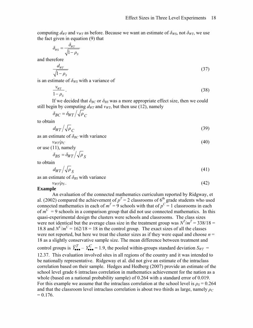
which can then be inserted into equation (18) or (31) along with ρS and ρC to obtain dWT. This estimate of dWT can then be inserted into equation (19) or (32) to obtain vWT, an estimate of the variance of dWT. Alternatively, suppose it is decided that the effect size δWC is appropriate because most other studies involve only a single site. We may begin by computing dWT and vWT as before. Because we want an estimate of δWC, not δWT, we use the fact given in equation (10) that
1
WTWC
S C
δδρ ρ
=− −
and therefore
1
WT
S C
dρ ρ− −
(35)
is an estimate of δWC with a variance of
1
WT
S C
vρ ρ− −
. (36)
Similarly, we might decide that δWS was a more appropriate effects size because most other studies involve schools that have several classrooms and nesting of students within classrooms is not taken into account in most of them. We may begin by
Effect Sizes in Three Level Experiments 18
computing dWT and vWT as before. Because we want an estimate of δWS, not δWT, we use the fact given in equation (9) that
1
WTWS
S
δδρ
=−
and therefore
1
WT
S
dρ−
(37)
is an estimate of δWS with a variance of
1
WT
S
vρ−
. (38)
If we decided that δBC or δBS was a more appropriate effect size, then we could still begin by computing dWT and vWT, but then use (12), namely BC WT Cδ δ ρ= to obtain
WT Cd ρ (39) as an estimate of δBC with variance vWT/ρC (40) or use (11), namely BS WT Sδ δ ρ= to obtain
WT Sd ρ (41) as an estimate of δBS with variance vWT/ρS . (42) Example An evaluation of the connected mathematics curriculum reported by Ridgway, et al. (2002) compared the achievement of pT = 2 classrooms of 6th grade students who used connected mathematics in each of mT = 9 schools with that of pC = 1 classrooms in each of mC = 9 schools in a comparison group that did not use connected mathematics. In this quasi-experimental design the clusters were schools and classrooms. The class sizes were not identical but the average class size in the treatment group was NT/mT = 338/18 = 18.8 and NC/mC = 162/18 = 18 in the control group. The exact sizes of all the classes were not reported, but here we treat the cluster sizes as if they were equal and choose n = 18 as a slightly conservative sample size. The mean difference between treatment and control groups is TY••• – = 1.9, the pooled within-groups standard deviation SCY••• WT = 12.37. This evaluation involved sites in all regions of the country and it was intended to be nationally representative. Ridgeway et al. did not give an estimate of the intraclass correlation based on their sample. Hedges and Hedberg (2007) provide an estimate of the school level grade 6 intraclass correlation in mathematics achievement for the nation as a whole (based on a national probability sample) of 0.264 with a standard error of 0.019. For this example we assume that the intraclass correlation at the school level is ρS = 0.264 and that the classroom level intraclass correlation is about two thirds as large, namely ρC = 0.176.

Effect Sizes in Three Level Experiments 19
The analysis ignored clustering and compared the mean of all of the students in the treatment with the mean of all of the students in the control group via a t-test, the t-value obtained was t = 3.488. This leads to a value of the standardized mean difference of
0 1536.T C
WT
Y Y S
••• •••−= ,
which is not an estimate of any of the three effect sizes considered here. If an estimate of the effect size δWT is desired, and we had imputed a school level intraclass correlation of ρS = 0.264 and a classroom level intraclass correlation of ρS = 0.176, then we use equation (31) to obtain dWT = (0.1536)(0.9811) = 0.1507. The effect size estimate is very close to the original standardized mean difference because the amount of clustering in this case is rather small. However even this small amount of clustering has a substantial effect on the variance of the effect size estimate. The variance of the standardized mean difference ignoring clustering is
2324 162 0 1536 0 009259
324 162 2 324 162 2. .
* ( )+
+ =+ −
.
However, computing the variance of dWT using equation (32) with ρS = 0.264 and ρS = 0.176, we obtain a variance estimate of 0.093295, which is more than 10 times the variance ignoring clustering. It is worth noting that if we had used the conservative approximation for vWT given in (33), we would have obtained a variance estimate of 0.093895, which differs from the computation given (32) by less than 1 percent. A 95 percent confidence interval for δT is given by 0 4480 0 1507 1 96 0 093295 0 1507 1 96 0 093295 0 7494T. . . . δ . . . .− = − ≤ ≤ + = . If clustering had been ignored in computing the variance of dWT, the confidence interval for the population effect size would have been -0.0382 to 0.3395. If we wanted to estimate δWC, then an estimate of δWC given by expression (35) is
0 1507 0 20141 0 264 0 176
. .. .
=− −
,
with variance given by expression (36) as 0.093295/(1 – 0.264 – 0.176) = 0.166598. If an estimate of δWS was wanted, then an estimate of δWS could be computed from expression (37) as
0 1507 0 17571 0 264
. ..
=−
,
with variance given by expression (38) as 0.093295/(1 – 0.264) = 0.126759. If we decided that δBC was a more appropriate effect size, an estimate could be computed from (39) as
0 1507 0 176 0 3592. . .= , with variance given by expression (40) as 0.093295/0.176 = 0.53008. If we decided that δBS was a more appropriate effect size, an estimate could be computed from (41) as

Effect Sizes in Three Level Experiments 20
0 1507 0 264 0 2933. . .= , with variance computed from (42) as 0.093295/0.264 = 0.353389. Is it Really Necessary to Take Both Levels of Clustering Into Account?
One might be tempted to think that accounting for clustering at one the highest level (e.g. schools) would be sufficient to account for most of the effects of clustering at both levels. Indeed there is a widely held belief among some researchers that only the highest level of clustering matters in analysis, and that lower levels of clustering can safely be omitted if they are not explicitly part of the analysis. Another belief that is sometimes cited is that any level of the design can be ignored if it is not explicitly included in the analysis. If this were the case the results of this paper might be theoretically interesting, but have few practical implications. It is clear from (15) and (17) that the effect size estimates dWS and dWT do not depend strongly on the intraclass correlation (at least within plausible ranges of intraclass correlations that are likely to be encountered in educational research). However, the analytic results presented here show that, in situations where there is a plausible amount of clustering at two levels, omitting either level of clustering from variance computations can lead to substantial biases in the variance of effect size estimators.
Table 2 shows some calculations of the variance of the effect size estimate dWT and its variance in a balanced design with m = 10, n = 20, ρS = 0.15, ρC = 0.10, and dWT = ( )/T C
WTT T S••• •••− = 0.15 (fairly typical values). Omitting the classroom (lowest level) of clustering leads to underestimates of the variance when the number of classrooms (lower level clusters) per school is small, underestimation that become less serious as the number of classrooms per school increases. For example, omitting the classroom level of clustering from variance computations leads to underestimation of the variance of dWT by 22% when p = 2, but by only 11% when p = 5. Because the number of classrooms per school is typically small in educational experiments, we judge that variance is likely to be seriously underestimated when the classroom level is ignored in computing variances of effect size estimates in three level designs.
The table shows that omitting the school (highest level) of clustering leads to larger underestimates of variance when the number of classrooms (lower level clusters) per school is small, which become even more serious when the number of classrooms becomes larger. Omitting the school level of clustering from variance computations leads to underestimation of the variance of dWT by about 67% when p = 2, but by 84% when p = 5.
One potential substitute for computing variances using the formulas for two levels of clustering is to compute the variances assuming two levels of clustering, but use a composite intraclass correlation that “includes” both between-school and between-class components. Table 2 shows that using only the school level of clustering to compute the variance of dWT but using ρ = ρS + ρC in place of the school level intraclass correlation performs poorly, leading to overestimates of the variance of from 23% (for p = 2) to 45% (for p = 5). However, using only the school level of clustering to compute the variance of dWT but using ρ = ρS + ρC /p in place of the school level intraclass correlation performs much better, leading to overestimates of the variance of less than 1% for all p.
Effect Sizes in Three Level Experiments 21
Conclusions This paper has provided definitions of five different effect sizes that can be estimated in three level studies using cluster randomization. Methods of estimation are provided for each effect size, and the sampling variances are also given. The sampling distribution of each estimator is shown to be a constant times a noncentral t-distribution and simple normal approximations are given in each case. Because these approximations have been extensively studied in the context of simpler effect size estimates and power analysis, there is reason to believe that they are reasonably accurate unless sample sizes are quite small (which is unlikely in cluster randomized designs). Simulation studies (reported in other studies) evaluating the accuracy of these approximations confirm expectations.
The analytic work shows that while clustering has only a small effect on the estimates of effect size involving between-student standard deviations, it can have a substantial effect on the variance of these effect size estimates. The example provided illustrates that small, but plausible, amounts of clustering can have a very large effect on the variance of effect sizes and therefore on confidence intervals in practical situations. This implies that ignoring clustering can have serious effects in meta-analysis, leading to serious underestimates of uncertainty in effect size estimates. Moreover, when the sampling design involves two levels of clustering (such as schools and classrooms), it appears that simply ignoring one of the levels of clustering in computing the variances of effect size estimates can also lead to marked underestimates of the variance of effect size estimates.
The results given in this paper can be used to estimate the effect sizes (and their variances) in cluster randomized trials that have been improperly analyzed by ignoring clustering, provided an intraclass correlation is known or can be imputed. The effect size estimates can then be used in meta-analyses along with any other effect size estimates of the same conceptual parameter, using the variances of the estimates to compute weights in the usual way, and using those weights in fixed or mixed effects analyses.
The results given in this paper require that a value of the intraclass correlation parameters ρS and ρC be known or imputed for sensitivity analysis. In some cases external data about ρS and ρC may be available (e.g., from previous studies or compendia such as that of Hedges and Hedberg, 2007). It is important to use external values of ρS and ρC with considerable caution, because the values of ρS and ρC have substantial influence on the results of analyses. In particular, it would be difficult to justify the use of the methods described in this paper using estimates of ρS and ρC obtained from small samples (small numbers of clusters) because those estimates are likely to be subject to considerable sampling error. Similarly, it would be difficult to justify the use of external estimates of ρS and ρC, even from large sample sizes if those estimates were not based on a similar sampling strategy, with similar populations, and similar outcome measures. However, making no correction for the effects of clustering at all corresponds to assuming that ρC = ρS = 0. The assumption that ρS = ρC = 0 is often very far from the case and thus it may introduce more serious biases in the computation of variances than using values of ρ that are slightly in error.
A major practical problem is that while there is rather extensive reference data on school level intraclass correlations (ρS), the data on classroom level intraclass correlations (ρC) is less extensive. Such data, either computed from surveys or from reports of

Effect Sizes in Three Level Experiments 22
experiments themselves, is badly needed to improve the meta-analysis of studies with multiple levels of clustering. Moreover, given the connection between effect sizes and statistical power, we speculate that our findings about the variance of effect size estimates imply that computations of statistical power in three level designs by omitting levels of clustering (that is, compute power in three level designs as if there were only two levels) will badly underestimate power in plausible situations. If this is so, information on classroom level intraclass correlations may be as crucial for planning of educational experiments that assign schools to treatments as well as for computing effect sizes.

Effect Sizes in Three Level Experiments 23
Appendix: Derivation of Sampling Distributions of Effect Size Estimates The sampling distribution of the effect size estimates proposed in this paper all follow from the same theorem, which was proven in Hedges (in press) and is restated below. Theorem: Suppose that Y ~ N(μ, aσ2/ ) and that SN% 2 is a quadratic form in normal variables that is independent of Y, so that E{S2} = bσ2, and V{S2} = 2cσ4, where a, b, c, and are constants. Then N%
Nb YTa S
⎛ ⎞= ⎜ ⎟⎝ ⎠
%
has approximately the noncentral t-distribution with b2/c degrees of freedom and noncentrality parameter
Nb μ Nbθ δa aσ
⎛ ⎞= =⎜ ⎟⎝ ⎠
% %,
where δ = μ/σ. Consequently
Y b aD TS N
= =%
(A1)
is a consistent estimate of the effect size δ with approximate variance
2
2a cδN b+
%. (A2)
The theorem can be applied to obtain the sampling distribution of each of the effect size estimators given in this paper, using some elementary facts. In each case we
apply the theorem with T CY Y Y••• •••= − , T Cμ μ μ•• •= − • , and = NN% TNC/(NT + NC), but with different definitions of S and σ (which imply different choices of the constants a, b, and c). In each case, we use the fact that the expected value of the mean difference is given by
{ }T C TY Y Cμ μ••• ••• •• ••− = −E
However the variance of variance of TY Y C••• •••− and the mean and variance of various
choices of S require different derivations in the balanced (equal cluster sample size) and unbalanced (unequal cluster sample size) cases. Equal Cluster Sample Sizes In the case of equal cluster sample sizes, a direct argument gives the variance of the mean difference as
{ } ( ) ( )
( ) [ ]
1 2 2 2
1 2 1 ( 1) ( 1)
T CWC BC BS
WT C S
Y Y N n np
N n ρ pn ρ
σ σ σ
σ
−••• •••
−
− = + +
= + − + −
V %
%. (A3)
We also use the moments of SBS2, SBC
2, SWC2, SWS
2, and SWT2, which are derived
from their relation to sums of squares in the analysis of variance (see, e.g., Snedecor, 1956). The design described here has a treatment factor with schools (nested within treatments) and classrooms (nested within schools and treatments) as nested factors. Using the expected mean squares from a design with one crossed factor and two nested

Effect Sizes in Three Level Experiments 24
factors, where both nested factors are considered random effects (see, e.g., Kirk, 1995, p.488) we have E{MSBS} = σWC
2 + nσC2 + pnσS
2 = σWT2[ 1 + (n – 1)ρC + (pn – 1) ρS],
E{MSBC} = σWC2 + nσC
2 = σWT2[1 + (n – 1)ρC – ρS],
and E{MSWC} = σWC
2 = σWT2[1 – ρC – ρS].
A standard result from analysis of variance of this design, is that the sums of squares divided by their expectations are independently distributed as chi-squares. In particular, SSBS / σWT
2[ 1 + (n – 1)ρC + (pn – 1) ρS] ~ χ(M – 2)2,
SSBC / σWT2[ 1 + (n – 1)ρC – ρS] ~ χM(p – 1)
2 , and
SSWC / σWT2[ 1 – ρC – ρS] ~ χMp(n – 1)
2 . Therefore, because the expected value of a chi-square equals its degrees of freedom, it follows that the expectations of the sums of squares are E{SSBS} = σWT
2(M – 2) [ 1 + (n – 1)ρC + (pn – 1) ρS], E{SSBC} = σWT
2M(p – 1)[ 1 + (n – 1)ρC – ρS], and E{SSWC} = σWT
2Mp(n – 1)[ 1 – ρC – ρS]. Because the variance of a chi-square equals twice its degrees of freedom, it follows that the variances of the sums of squares are V{SSBS} = 2σWT
4(M – 2) [ 1 + (n – 1)ρC + (pn – 1) ρS]2, V{SSBC} = 2σWT
4M(p – 1)[ 1 + (n – 1)ρC – ρS]2, and V{SSWC} = 2σWT
4Mp(n – 1)[ 1 – ρC – ρS]2. Using these results, we obtain the expected value and variance of the five sample variances involved in the expressions for the effect size estimates described in this paper. Because SWC
2 = SSWC/(N – Mp), it follows that the expected value and variance of SWC2
are
{ } (2 2 1WC WT C SE S )ρ ρσ= − − (A4)
and
{ } ( )24 42 2 1 2WT C S WCWC
ρ ρV S
N Mp N Mpσ σ− −
=− −
= . (A5)
Because SBC2 = SSBC/M (p – 1) n, it follows that the expected value and variance of SBC
2 are
{ } [2 2 1 ( 1)BC WT CE S n ]ρ / nσ= + − (A6)
and
{ } [ ]( )
242
22 1 ( 1)WT C
BCn ρ
V SMp M n
σ + −=
−. (A7)
Because SBS2 = SSBS/(M – 2)np, it follows that the expected value and variance of SBS
2 are
{ } [2 2 1+ ( 1) ( 1) BS WT C SE S n ]ρ pn ρ / npσ= − + − (A8)
and

Effect Sizes in Three Level Experiments 25
{ } [ ]( )
242
2 22 1+ ( 1) ( 1)
2WT C S
BSn ρ pn ρ
V SM n p
σ − + −=
−. (A9)
The expectations and variances of these sums of squares permit computation of the expectations and variances of the composite sums of squares SSWS and SSWT and the variances SWS
2 and SWT2. Because SWS
2 = (SSWC + SSBC)/(N – M), it follows that the expected value and variance of SWS
2 are
{ } ( ) ( )( )( )
2 2 21 11 1
1 1C CWS WT S WS
S
n ρ n ρE S ρ
pn ρ pnσ σ
1⎡ ⎤⎡ ⎤− −
= − − = −⎢ ⎥⎢ ⎥− − −⎢ ⎥⎣ ⎦ ⎣ ⎦ (A10)
and
{ }( )
( ) ( )
4 22
2
4 2
22
2 ( 1) 2 1 1
1
2 ( 1) 2 1 1
1 1
2 2WT C C
WS
2 2WS C C
S
pn ρ n( p )ρρ n ( p )ρV S
M pn
pn ρ n( p )ρρ n ( p )ρ
M pn ρ
σ
σ
⎡ ⎤− + − + −⎣ ⎦=−
⎡ ⎤− + − + −⎣ ⎦=− −
. (A11)
Because SWT2 = (SSWC + SSBC + SSBS)/(N – 2), it follows that the expected value
and variance of SWT2 are
{ }2 2 2( 1) 2( 1)12
SWT WT
pn Cρ n ρE SN
σ− − −⎛= −⎜ −⎝ ⎠
⎞⎟ (A12)
and
{ } ( )( )
4 2 2 22
2
2 ( 2) 2 2
2
WT S C S C S CWT
pnNρ nNρ N ρ nNρ ρ Nρ ρ+2Nρ ρV S
N
σ + + − + +=
−
) ( ) ) (
, (A13)
where N)
= (N – pn), = (N – 2n), andN(
ρ = 1 – ρS – ρC. The distribution of dWC. In this case we apply the theorem with σ2 = σWC
2 and S2 = SWC
2. Here
2 2 2
21 ( 1) ( 1)
1WC BC BS C S
C SWC
n np n ρ pn ρaρ ρ
σ σ σσ
+ + + − + −= =
− −.
Because the expected value of SWC2 is σWC
2it follows that b = 1. Because the variance of SWC
2 is 2σWC4/(N – Mp), it follows that c = 1/(N – Mp). Substituting the expressions for a,
b, and c into (A1) and (A2), and simplifying, gives the results in expressions (13) and (14). Since S2 involves only a single chi-square, it follows that the t-statistic corresponding to dWC has exactly the noncentral t-distribution with (N – Mp) degrees of freedom. The distribution of dWS. In this case we apply the theorem with σ2 = σWS
2 = σWC2 +
σBS2 and S2 = SWS
2. Here
2 2 2
21 ( 1) ( 1)
1WC BC BS C S
SWS
n np n ρ pn ρaρ
σ σ σσ
+ + + − + −= =
−,

Effect Sizes in Three Level Experiments 26
{ } ( )
( )( )
2
21
1 11WS C
SWS
E S n ρb
ρ pnσ
−= = −
− −,
and
{ }
( )( )
2 2
4 2( 1) ( 1) ( 1)
2 1 1
2 2WS C C
WS S
V S pn ρ n p ρρ n p ρcM pn ρσ
− + − + −= =
− −.
Substituting the expressions for a, b, and c into (A1) and (A2), and simplifying, gives the results in expressions (15) and (16). The distribution of dWT. In this case we apply the theorem with σ2 = σWT
2 and S2 = SWT
2. Here
2 2 2
2 1 ( 1) ( 1)WC BC BSC S
WT
n pna n ρ pn ρσ σ σσ
+ += = + − + − .
Using the expected value of SWT2 given in (A12), we compute
{ }2
22( 1) 2( 1)1
2WT S C
WT
E S pn ρ n ρbNσ
− + −= = −
−,
and using the variance of SWT2 given in (A13), we compute
{ }
( )
2 2 2 2
4 2( 2) 2 2
2 2
WT S C S C S C
WT
V S pnNρ nNρ N ρ nNρ ρ Nρ ρ+2Nρ ρcNσ
+ + − + += =
−
) ( ) ) (
.
Substituting the expressions for a, b, and c into (A1) and (A2), and simplifying, gives the results in expressions (17) and (18). The distribution of dBC. In this case we apply the theorem with σ2 = σBC
2 and S2 = SBC
2. Here 2 2 2
21 ( 1) ( 1)
1WC BC BS C S
CBC
n pn n ρ pn ρaρ
σ σ σσ
+ + + − + −= =
−,
{ }2
21 ( 1)BC S C
CBC
E S ρ n ρbnρσ
− − −= = ,
and
{ } [ ]2 2
2 21 ( 1)
( 1)
BC S C
BC C
V S ρ n ρc
M p n ρσ
− + −= =
− 2 .
Substituting the expressions for a, b, and c into (A1) and (A2), and simplifying, gives the results in expressions (19) and (20). Since S2 involves only a single chi-square, it follows that the t-statistic corresponding to dBC has exactly the noncentral t-distribution with M(p – 1) degrees of freedom. The distribution of dBS. In this case we apply the theorem with σ2 = σBS
2 and S2 = SBS
2. Here

Effect Sizes in Three Level Experiments 27
2 2 2
21 ( 1) ( 1)
1WC BC BS C S
SBS
n pn n ρ pn ρaρ
σ σ σσ
+ + + − + −= =
−,
{ }2
21 ( 1) ( 1)BS C S
SBS
E S n ρ pn ρbpnρσ
− − − −= = ,
and
{ } [ ]2 2
4 2 21 ( 1) ( 1)
2 ( 2)
BS S C
BS S
V S pn ρ n ρc
M p n ρσ
− − + −= =
− 2 .
Substituting the expressions for a, b, and c into (A1)and (A2), and simplifying, gives the results in expressions (21) and (22). Since S2 involves only a single chi-square, it follows that the t-statistic corresponding to dBS has exactly the noncentral t-distribution with M – 2 degrees of freedom. Unequal Cluster Sample Sizes When cluster sample sizes are unequal, expressions for the effect size estimators and their variances are more complex. We first derive the variance of the mean differences. A direct argument leads to
{ } ( ) [11 ( 1) ( 1)T C
U S U CY Y N p ]ρ n ρ−
••• •••− = + − + −%V (A14)
where pU and nU are defined by (24) and (25) respectively. The expected value and variance of SWS
2and SWT2 can be calculated from the analysis of variance across
classrooms within schools and across schools within the treatment groups. When cluster sample sizes are unequal, the between school, between classroom, and within classroom sums of squares are still independent, and the within classroom sum of squares has a chi-square distribution, but if school and classroom sample sizes are unequal, the between school and between classroom sums of squares do not, in general, have chi-square distributions. However because both of these sum of squares are quadratic forms, the methods used in this paper apply and the distribution of effect size estimates can be obtained. The distribution of dWC. In this case, we apply the theorem with σ2 = σWC
2 and S2 = SWC
2. Here
2 2 2
21 ( 1) ( 1)
1WC U BS U BC S C
S CWC
p n pn ρ n ρaρ ρ
σ σ σσ
+ + + − + −= =
− −.
Because SWC2 is the same whether school or classroom sample sizes are equal or not, it
follows that b = 1and c = 1/(N – NS). Substituting the expressions for a, b, and c into (A1) and (A2), and simplifying, gives the results in expressions (13) and (23). Since S2 involves only a single chi-square, it follows that the t-statistic corresponding to dWC has exactly the noncentral t-distribution. with (N – NS) degrees of freedom. The distribution of dWS. In this case we apply the theorem with σ2 = σWS
2 = σWC2 +
σBS2 and S2 = SWS
2. Here
2 2 2
21 ( 1) ( 1)
1WC U BC U BS U C U S
SWS
n p n ρ p ρaρ
σ σ σσ
+ + + − + −= =
−.

Effect Sizes in Three Level Experiments 28
We obtain the expected value and variance of SWS2 by using the fact that
2
2
T T C
WSSSB SSW SSB SSWS
N+ + +
=−
C
,
where SSBCT and SSWCT and SSBCC and SSWCC are the sums of squares between and within classes in the treatment and control groups, respectively. Using the expected values of the SSBC’s and SSWC’s given, for example, on page 429 of Searle, Casella, and McCulloch (1992), we obtain (in our notation)
{ }2
2 ( )( )
2 BCWS WC
N Mn σE S σN M−
= +−%
,
so that
{ }2
C2
( )1( 1)(1
WS
S SWS
E S n 1bN
ρ)ρσ
−= = −
− −%
.
Because the between clusters variance component estimates in the treatment and control groups are
( )2T T
TBC T
MSBC MSWCˆn
σ −=
%
and
( )2C C
CBC C
MSBC MSWCˆn
σ −=
%,
it follows that SWS2 can be written as a function of between and within cluster variance
components
( ) ( ) ( ) ( )2 2 2
2( ) ( )T T T C C C T T C C
WC WC BC BCWS
ˆ ˆ ˆN M N M B BS
N M
σ σ σ− + − + +=
−
2σ̂
,
where BT = NT – /MTn% T and BC = NC – /MCn% C. Therefore the variance of SWS2 is given by
( ) { } ( ) ( )
( ) ( ) ( ) ( )
( ) ( ) ( ) ( )
2 22 2 2 2
2 2 2 2
2 2 2 2
V ( ) V ( ) V
V V
2( ) Cov 2( ) Cov
T T T C C CWS WC WC
T T C CBC BC
T T T T T C C C C CWC BC WC BC
ˆ ˆN M S N M N M
ˆ ˆB B
ˆ ˆ ˆ ˆN M B , N M B ,
⎧ ⎫ ⎧ ⎫− = − + −⎨ ⎬ ⎨ ⎬
⎩ ⎭ ⎩ ⎭⎧ ⎫ ⎧ ⎫
+ +⎨ ⎬ ⎨ ⎬⎩ ⎭ ⎩ ⎭
⎛ ⎞ ⎛ ⎞+ − + −⎜ ⎟ ⎜ ⎟
⎝ ⎠ ⎝ ⎠
σ σ
σ σ
σ σ σ σ
.
Using the expressions for the variances and covariances of the variance component estimates on page 430 of Searle, Casella, and McCulloch (1992), simplifying, and substituting into the formula for c yields
{ }
( )( )
2 2
4 2( 1) ( 1) ( 1)
2 1 1
2 2WS C C
WS S
V S pn ρ n p ρρ n p ρcM pn ρσ
− + − + −= =
− −.
Substituting the expressions for a, b, and c into (A1) and (A2), and simplifying, gives the results in expressions (26) and (28).

Effect Sizes in Three Level Experiments 29
The distribution of dWT. In this case, we apply the theorem with σ2 = σWT2 and S2 =
SWT2. We obtain the expected value and variance of SWT
2 by using the fact that
2
2
T T T C C
WTSSBS SSBC SSWC SSBS SSBC SSWCS
N+ + + + +
=−
C
,
where SSBST, SSBCT, and SSWCT and SSBSC, SSBCC and SSWCC are the sums of squares between schools, between classes, and within classes in the treatment and control groups, respectively. Using the expected values of the SSBS’s, SSBC’s, and SSWC’s given, for example, on page 429 of Searle, Casella, and McCulloch (1992), we obtain the expected value and variance of SWT
2. Here
2 2 2
2 1 ( 1) ( 1)WC U BS U BCU S U
WT
p na p Cρ n ρσ σ σσ
+ += = + − + −
and
{ }2
22 1 2 11
2WT U S U
WT
E S ( p ) Cρ ( n )bN
ρσ
− + −= = −
−.
The exact variance of S2 is quite complex, therefore we substitute pU for pn and nU for n into expression (A13) to obtain the approximate variance of SWT
2, use this approximate variance to obtain the constant c in the second term of the variance of dWT. Substituting the expressions for a, b, and c into (A1) and (A2), and simplifying, gives the results in expressions (31) and (32).

Effect Sizes in Three Level Experiments 30
References
Box, G. E. P. (1954). Some theorems on quadratic forms applied to the study of analysis of variance problems, I. Effect of inequality of variance in the one-way classification. Annals of Mathematical Statistics, 25, 290-302.
Bryk, A. & Schneider, B. (2000). Trust in schools. New York: Russell Sage Foundation. Donner, N., Birkett, N., & Buck, C. (1981). Randomization by cluster. American Journal
of Epidemiology, 114, 906-914. Donner, A. & Klar, N. (2000). Design and analysis of cluster randomization trials in
health research. London: Arnold. Donner, A. & Klar, N. (2002). Issues in the meta-analysis of meta-analysis of cluster
randomized trials. Statistics in Medicine, 21, 1971-2980. Dunkin, M. J. & Biddle, B. J. (1974). The study of teaching. New York: Holt, Rinehardt,
and Winston. Geisser, S. & Greenhouse, S. W. (1958). An extension of Box’s results on the use of the
F distribution in multivariate analysis. Annals of Mathematical Statistics, 29, 885-891.
Guilliford, M. C., Ukoumunne, O. C., & Chinn, S. (1999). Components of variance and intraclass correlations for the design of community-based surveys and intervention studies. Data from the Health Survey for England 1994. American Journal of Epidemiology, 149, 876-883.
Hedges, L. V. & Hedberg, E. C. (2007). Intraclass correlation values for planning group randomized experiments in education. Educational Evaluation and Policy Analysis, 29, 60-87.
Hedges, L. V. (1981). Distribution theory for Glass’s estimator of effect size and related estimators. Journal of Educational Statistics, 6, 107-128.
Hedges, L. V. (in press). Effect sizes in cluster randomized designs. Journal of Educational and Behavioral Statistics.
Hopkins, K. D. (1982). The unit of analysis: Group means versus individual observations. American Educational Research Journal, 19, 5-18.
Kirk, R. (1995). Experimental design. Belmont, CA: Brooks Cole. Kish, L. (1965). Survey sampling. New York: John Wiley. Klar, N. & Donner, A. (2001). Current and future challenges in the design and analysis of
cluster randomization trials. Statistics in Medicine, 20, 3729-3740. Laopaiboon, M. (2003). Meta-analyses involving cluster randomization trials: A review
of published literature in health care. Statistical Methods in Medical Research, 12, 515-530.
Murray, D. M. & Blitstein, J. L. (2003). Methods to reduce the impact of intraclass correlation in group-randomized trials, Evaluation Review, 27, 79-103.
Murray, D. M., Varnell, S. P., & Blitstein, J. L. (2004). Design and analysis of group-randomized trials: A review of recent methodological developments. American Journal of Public Health, 94, 423-432.
Nye, B., Hedges, L. V., & Konstantopoulos, S. (2004). How large are teacher effects? Educational Evaluation and Policy Analysis, 26, 237-257.
Raudenbush, S. W. & Bryk, A. S. (2002). Hierarchical linear models. Thousand Oaks, CA: Sage Publications.

Effect Sizes in Three Level Experiments 31
Rooney, B. L. & Murray, D. M. (1996). A meta-analysis of smoking prevention programs after adjustment for errors in the unit of analysis. Health Education Quarterly, 23, 48-64.
Searle, S. R. (1971). Linear models. New York: John Wiley. Searle, S. R., Casella, G., & McCulloch, C. E. (1992). Variance components. New York:
John Wiley. Snedecor, G. W. (1956). Statistical methods applied to experiments in agriculture and
biology. Ames, IA: Iowa State University Press. Verma, V. & Lee, T. (1996). An analysis of sampling errors for demographic and health
surveys. International Statistical Review, 64, 265-294.

Table 1 School and classroom level intraclass correlations estimated from STAR and NAEP Mathematics Reading Grade ρS ρC ρC/ρS ρS ρC ρC/ρS
K (STAR) 0.17 0.13 0.76 0.17 0.11 0.69 1 (STAR) 0.18 0.13 0.74 0.18 0.08 0.46 2 (STAR) 0.16 0.12 0.74 0.15 0.10 0.64 3 (STAR) 0.15 0.11 0.74 0.11 0.09 0.77 4 (NAEP 1992) 0.24 0.14 0.59 0.22 0.12 0.53 4 (NAEP 1996) 0.29 0.13 0.45 0.24 0.09 0.40 Note: The intraclass correlations in STAR are computed from data in Nye, Konstantopoulos, And Hedges (2004).
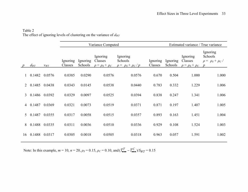
Effect Sizes in Three Level Experiments 33
Table 2 The effect of ignoring levels of clustering on the variance of dWT Variance Computed Estimated variance / True variance
p dWT vWT Ignoring Classes
Ignoring Schools
Ignoring Classes ρ = ρS + ρC
Ignoring Schools ρ = ρS + ρC / p
Ignoring Classes
Ignoring Schools
Ignoring Classes ρ = ρS + ρC
Ignoring Schools ρ = ρS + ρC / p
1 0.1482 0.0576 0.0385 0.0290 0.0576 0.0576 0.670 0.504 1.000 1.000
2 0.1485 0.0438 0.0343 0.0145 0.0538 0.0440 0.783 0.332 1.229 1.006
3 0.1486 0.0392 0.0329 0.0097 0.0525 0.0394 0.838 0.247 1.341 1.006
4 0.1487 0.0369 0.0321 0.0073 0.0519 0.0371 0.871 0.197 1.407 1.005
5 0.1487 0.0355 0.0317 0.0058 0.0515 0.0357 0.893 0.163 1.451 1.004
8 0.1488 0.0335 0.0311 0.0036 0.0510 0.0336 0.929 0.108 1.524 1.003
16 0.1488 0.0317 0.0305 0.0018 0.0505 0.0318 0.963 0.057 1.591 1.002 Note: In this example, m = 10, n = 20, ρS = 0.15, ρC = 0.10, and ( )/ = 0.15 T C
WTT T S••• •••−