Effect of viscosity, capillarity and grid spacing on thermal variable-density flow

Journal of Hydrology 400 (2011) 41–57

Contents lists available at ScienceDirect

Journal of Hydrology

journal homepage: www.elsevier .com/ locate / jhydrol

Effect of viscosity, capillarity and grid spacing on thermal variable-density flow

Thomas Graf a,⇑, Michel C. Boufadel b

a Institute of Fluid Mechanics, Department of Civil Engineering, Leibniz University Hannover, Appelstraße 9 A, 30167 Hannover, Germanyb College of Engineering, Department of Civil and Environmental Engineering, Temple Universität, 1947 N. 12th Street, Philadelphia, PA, USA

a r t i c l e i n f o

Article history:Received 12 March 2010Received in revised form 8 December 2010Accepted 19 January 2011Available online 3 February 2011

This manuscript was handled by P. Baveye,Editor-in-Chief

Keywords:DensityViscosityUnsaturatedElder problemCapillarityHeat flow

0022-1694/$ - see front matter � 2011 Elsevier B.V. Adoi:10.1016/j.jhydrol.2011.01.025

⇑ Corresponding author. Tel.: +49 (0) 511/762 4786E-mail address: [email protected]

s u m m a r y

The HydroGeoSphere model is further developed and used to investigate the effects of viscosity, capillarityand grid spacing on thermal variable-density flow. Under saturated and unsaturated flow conditions, theflow dynamics significantly depends on the viscosity assumption (constant vs. variable), where downwel-ling regions (constant viscosity) become upwelling regions (temperature-dependent variable viscosity).Capillarity does not change the location of downwelling and upwelling regions. Capillarity can significantlyalter the flow dynamics in the way that the water table acts as a ‘‘lid’’ to flow, and it diverts a thermal plumelaterally. Significance of capillarity increases with increasing soil moisture. Thermal convective flow ishighly sensitive to spatial discretization. While the flow dynamics remains to be a function of grid level,spatial discretization Dx = Dz = 1 m appears to be appropriate to simulate unsaturated variable-densityflow and heat transfer in porous media because estimated errors have asymptotically reached a minimum.

� 2011 Elsevier B.V. All rights reserved.

1. Introduction

Temperature variations in the subsurface can significantly alterwater density and viscosity in both the unsaturated soil zone andin the saturated groundwater zone. Examples of heat sinks or sourcesin the subsurface are (i) geothermal activity, (ii) solar radiation, (iii)radioactive, heat-producing waste repositories, (iv) underground en-ergy storage, (v) underground storage of hot or cold materials, (vi)buried electric cables and steam pipes, and (vii) disposal of wasteheat from power plants. As a result, non-isothermal conditions ofpartially saturated systems are common, which can affect water flowunder capillary and gravitational forces. Another example of high-density flow in unsaturated media is ‘‘frac fluid’’ used to create frac-tures in the Marcellus Shale formation for extraction of natural gas(methane) in Pennsylvania and New York. The frac fluid is storedin open ponds, and it is important to understand in what way themovement of leaking frac fluid in the formation is affected by fluiddensity, viscosity and temperature. For example, would a leak bemore devastating in summer or in winter? Clearly, the effects of tem-perature variations on variable-density, variable-viscosity flow de-pend on the spatial scale regarded. In the present study, we willfocus on process that occur on the large reservoir scale.

Small-scale (meter) effects of temperature have been studied byBear and Gilman (1995) and Grifoll et al. (2005). Bear and Gilman

ll rights reserved.

; fax: +49 (0) 511/762 3777.(T. Graf).

(1995) have presented an exhaustive study of the migration of saltin the unsaturated zone caused by heating. It was found that a heatsource in an unsaturated soil attracts dissolved salt and, at temper-atures above 50–70� may cause precipitation of salt. While Bearand Gilman (1995) focused on heat transfer by conduction andthe associated reactive transport of salt, heat transfer by convec-tion was not considered. Free convective flow patterns in partiallysaturated systems caused by heating were not investigated. Freethermal convection, however, is a key process in geothermal reser-voirs, and it should be understood in more detail. Grifoll et al.(2005) have presented a model formulation for coupled transportof liquid and vapor water, and energy in unsaturated porous mediato describe non-isothermal water transport in the unsaturated soilzone. Grifoll et al. (2005) have concentrated on the effect of evap-oration on non-isothermal soil water flow, which is a relevantprocess on the meter-scale. However, on the larger kilometer-scaleof a geothermal reservoir regarded here, the effect of viscosity,density and capillarity can be expected to be more important tocharacterize non-isothermal fluid flow.

Variable-density fluid flow on the large (kilometer) scale ismostly dominated by free convection. Large vertical temperaturedifferences create significant density gradients that can drive fluidflow. Using the example site at Soultz-sous-Forêts, France, Batailléet al. (2006) have shown that free thermal convection in geother-mic reservoirs is possible. When free convection occurs, zones ofupwelling hot fluid and zones of downwelling cold fluid alternate.Fascinating thermal convective flow patterns can also be observed

http://dx.doi.org/10.1016/j.jhydrol.2011.01.025

mailto:[email protected]

http://dx.doi.org/10.1016/j.jhydrol.2011.01.025

http://www.sciencedirect.com/science/journal/00221694

http://www.elsevier.com/locate/jhydrol

42 T. Graf, M.C. Boufadel / Journal of Hydrology 400 (2011) 41–57

using the Elder (1967) problem of free thermal convection(Oldenburg et al., 1995). Elder (1967) has studied density-driventhermal convection in fully saturated porous media due to nonuni-form heating of a vertical 2-D domain from below. The thermalElder problem, as well as its haline analog (Diersch, 1981; Vossand Souza, 1987) have been numerically simulated numeroustimes (e.g. Voss and Souza, 1987; Frolkovic and De Schepper,2001; Diersch and Kolditz, 2002; Simpson and Clement, 2003; Grafand Therrien, 2005; Prasad and Simmons, 2005). The Elder prob-lem has become a very popular and often stressed benchmarkproblem in the water resources literature. Simulations of the Elderproblem indicate that (i) density gradients drive free convectiveflow, and (ii) the pattern of free convective flow is significantlycontrolled by the spatial grid used.

Boufadel et al. (1999b) have extended the haline analog of theElder problem for application to partially saturated systems. Itwas found that the free convective pattern is strongly dependenton the soil type, and that small relative permeability in sandy soilscan inhibit free convection in the unsaturated zone. While Boufadelet al. (1999b) regarded the haline analog of the Elder problem, thepresent study will concentrate on an extension of the original ther-mal Elder problem to partially saturated systems. We will focus onthe effects of viscosity variations, density variations, and spatialgridding on free convective thermal fluid flow. While grid spacingis known to affect haline convection in porous media, the effect ofgrid spacing on thermal convection is mostly unclear. This is thefirst study that examines the effect of capillarity and grid spacingon thermal variable-density variable-viscosity flow. Results of thepresent study are applicable to the numerical simulation of thermalfluid flow in (i) geothermal reservoirs, (ii) partially saturated soilsthat are subject to heating, and (iii) repositories for heat-producingradioactive waste.

2. Numerical model

2.1. Model development

2.1.1. Earlier FRAC3DVS/HydroGeoSphere versionHydroGeoSphere is a numerical variable-density, variably satu-

rated flow and solute transport model for porous and fractured-porous media, and it is based on the FRAC3DVS model (Therrienand Sudicky, 1996; Graf and Therrien, 2005). The HydroGeoSpheremodel applies the control volume finite element (CVFE) method tothe flow equation, the Galerkin finite element method with full up-stream weighting to the heat transfer equation, and a finite-differ-ence scheme to time derivatives. The spatiotemporally discretizedmatrix equations are solved using the WATSIT iterative solverpackage for general sparse matrices (Clift et al., 1996) and a conju-gate gradient stabilized (CGSTAB) acceleration technique (Rauschet al., 2005). More details on HydroGeoSphere are given in Therrienet al. (2009).

Earlier versions of the FRAC3DVS/HydroGeoSphere model simu-late the following three physical processes independently: (i)unsaturated–saturated flow (Therrien and Sudicky, 1996), (ii) var-iable-density flow (Graf and Therrien, 2005), and (iii) saturatedheat transfer (Graf and Therrien, 2007). The nonlinearity arisingfrom unsaturated–saturated flow (process i) has been linearizedby Newton iteration in Therrien and Sudicky (1996), and the non-linearity arising from variable-density flow (process ii) has beenlinearized by Picard iteration in Graf and Therrien (2005).

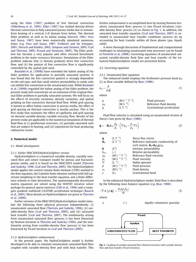
Fig. 1. Coupling of variably saturated flow (Newton iteration) with variable-densityflow and heat transfer (Picard iteration).

2.1.2. HydroGeoSphere enhancementIn the present paper, the HydroGeoSphere model is further

developed to be able to simulate unsaturated–saturated fluid flowcoupled with variable-density flow and with heat transfer. This

further enhancement is accomplished here by nesting Newton iter-ations (unsaturated flow; process (i) into Picard iterations (vari-able-density flow; process (ii) as shown in Fig. 1. In addition, thesaturated heat transfer equation (Graf and Therrien, 2007) is ex-tended to unsaturated heat transfer conditions (process iii) byaccounting for heat transfer within all three phases (gas, liquid,solid).

A more thorough discussion of fundamental and computationalchallenges in simulating unsaturated zone processes can be foundin Finsterle et al. (2008). Governing equations of unsaturated–sat-urated variable-density fluid flow and heat transfer of the en-hanced HydroGeoSphere model are presented below.

2.2. Governing equations

2.2.1. Unsaturated flow equationsThe enhanced model employs the freshwater pressure head w0

(L) as flow variable defined by Bear (1988):

w0 ¼p

q0gð1Þ

where

p
(M L�1 T�2) Fluid pressure q0 (M L�3) Reference fluid density g (L T�2) Gravitational acceleration
Fluid flow velocity is calculated using an unsaturated version ofDarcy’s law given by Bear (1988):

q ¼ �K0krwl0

l‘

� rw0 þq‘

q0rz

� �ð2Þ

where

q
(L T�1) Darcy flux vector K0 (L T�1) Reference hydraulic conductivity of
rock matrix; K0=kq0g/l0

k
(L2) Intrinsic permeability krw (–) Relative permeability l0 (M L�1 T�1) Reference fluid viscosity l‘ (M L�1 T�1) Fluid viscosity r (L�1) Nabla operator p (M L�1 T�2) Fluid pressure q‘ (M L�3) Fluid density z (L) Gravitational head
In the enhanced HydroGeoSphere model, fluid flow is describedby the following mass balance equation (e.g. Bear, 1988):

�r � q‘q� �

¼ @ð/q‘SwÞ@t

ð3Þ

where

/
(–) Aquifer volumetric porosity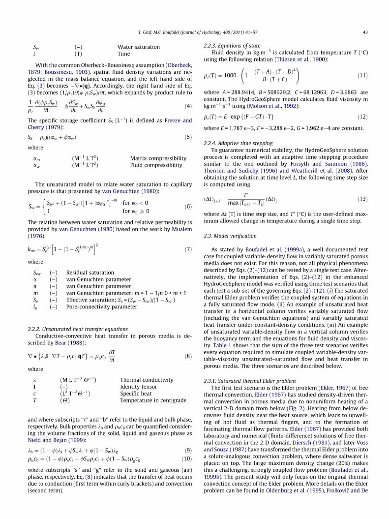

T. Graf, M.C. Boufadel / Journal of Hydrology 400 (2011) 41–57 43

Sw
(–) Water saturation t (T) Time
With the common Oberbeck–Boussinesq assumption (Oberbeck,
1879; Boussinesq, 1903), spatial fluid density variations are ne-glected in the mass balance equation, and the left hand side ofEq. (3) becomes �r�{q}. Accordingly, the right hand side of Eq.(3) becomes (1/q‘)@(/ q‘Sw)/@t, which expands by product rule to
1q‘

@ /q‘Swð Þ@t

¼ /@Sw

@tþ SwSS

@w0

@tð4Þ

The specific storage coefficient SS (L�1) is defined as Freeze andCherry (1979):

SS ¼ q0gðam þ /awÞ ð5Þ

where

am
(M�1 L T2) Matrix compressibility aw (M�1 L T2) Fluid compressibility
The unsaturated model to relate water saturation to capillarypressure is that presented by van Genuchten (1980):

Sw ¼Swr þ ð1� SwrÞ 1þ jaw0j

n� ��m for w0 < 01 for w0 P 0

(ð6Þ

The relation between water saturation and relative permeability isprovided by van Genuchten (1980) based on the work by Mualem(1976):

krw ¼ SðlpÞe 1� ð1� Sð1=mÞe Þm

h i2ð7Þ

where

Swr
(–) Residual saturation a (–) van Genuchten parameter n (–) van Genuchten parameter m (–) van Genuchten parameter; m = 1 � 1/n 0 < m < 1 Se (–) Effective saturation; Se = (Sw � Swr)/(1 � Swr) lp (–) Pore-connectivity parameter
2.2.2. Unsaturated heat transfer equationsConductive-convective heat transfer in porous media is de-

scribed by Bear (1988):

r � kbI � rT � q‘c‘ qT� �

¼ qbcb@T@t

ð8Þ

where

k
(M L T�3 H�1) Thermal conductivity I (–) Identity tensor c (L2 T�2H�1) Specific heat T (H) Temperature in centigrade
and where subscripts ‘‘‘’’ and ‘‘b’’ refer to the liquid and bulk phase,respectively. Bulk properties kb and qbcb can be quantified consider-ing the volume fractions of the solid, liquid and gaseous phase asNield and Bejan (1999):

kb ¼ ð1� /Þks þ /Swk‘ þ /ð1� SwÞkg ð9Þqbcb ¼ ð1� /Þqscs þ /Swq‘c‘ þ /ð1� SwÞqgcg ð10Þ

where subscripts ‘‘s’’ and ‘‘g’’ refer to the solid and gaseous (air)phase, respectively. Eq. (8) indicates that the transfer of heat occursdue to conduction (first term within curly brackets) and convection(second term).

2.2.3. Equations of stateFluid density in kg m�3 is calculated from temperature T (�C)

using the following relation (Thiesen et al., 1900):

q‘ðTÞ ¼ 1000 � 1� ðT þ AÞ � ðT � DÞ2

B � ðT þ CÞ

!ð11Þ

where A = 288.9414, B = 508929.2, C = 68.12963, D = 3.9863 areconstant. The HydroGeoSphere model calculates fluid viscosity inkg m�1 s�1 using (Molson et al., 1992):

l‘ðTÞ ¼ E � exp ðF þ GTÞ � Tf g ð12Þ

where E = 1.787 e�3, F = �3.288 e�2, G = 1.962 e�4 are constant.

2.2.4. Adaptive time steppingTo guarantee numerical stability, the HydroGeoSphere solution

process is completed with an adaptive time stepping proceduresimilar to the one outlined by Forsyth and Sammon (1986),Therrien and Sudicky (1996) and Weatherill et al. (2008). Afterobtaining the solution at time level L, the following time step sizeis computed using

ðDtÞLþ1 ¼T�

max jTLþ1 � TLjðDtÞL ð13Þ

where Dt (T) is time step size, and T⁄ (�C) is the user-defined max-imum allowed change in temperature during a single time step.

2.3. Model verification

As stated by Boufadel et al. (1999a), a well documented testcase for coupled variable-density flow in variably saturated porousmedia does not exist. For this reason, not all physical phenomenadescribed by Eqs. (2)–(12) can be tested by a single test case. Alter-natively, the implementation of Eqs. (2)–(12) in the enhancedHydroGeoSphere model was verified using three test scenarios thateach test a sub-set of the governing Eqs. (2)–(12): (i) The saturatedthermal Elder problem verifies the coupled system of equations ina fully saturated flow mode. (ii) An example of unsaturated heattransfer in a horizontal column verifies variably saturated flow(including the van Genuchten equations) and variably saturatedheat transfer under constant-density conditions. (iii) An exampleof unsaturated variable-density flow in a vertical column verifiesthe buoyancy term and the equations for fluid density and viscos-ity. Table 1 shows that the sum of the three test scenarios verifiesevery equation required to simulate coupled variable-density var-iable-viscosity unsaturated–saturated flow and heat transfer inporous media. The three scenarios are described below.

2.3.1. Saturated thermal Elder problemThe first test scenario is the Elder problem (Elder, 1967) of free

thermal convection. Elder (1967) has studied density-driven ther-mal convection in porous media due to nonuniform heating of avertical 2-D domain from below (Fig. 2). Heating from below de-creases fluid density near the heat source, which leads to upwell-ing of hot fluid as thermal fingers, and to the formation offascinating thermal flow patterns. Elder (1967) has provided bothlaboratory and numerical (finite-difference) solutions of free ther-mal convection in the 2-D domain. Diersch (1981), and later Vossand Souza (1987) have transformed the thermal Elder problem intoa solute-analogous convection problem, where dense saltwater isplaced on top. The large maximum density change (20%) makesthis a challenging, strongly coupled flow problem (Boufadel et al.,1999b). The present study will only focus on the original thermalconvection concept of the Elder problem. More details on the Elderproblem can be found in Oldenburg et al. (1995), Frolkovic and De

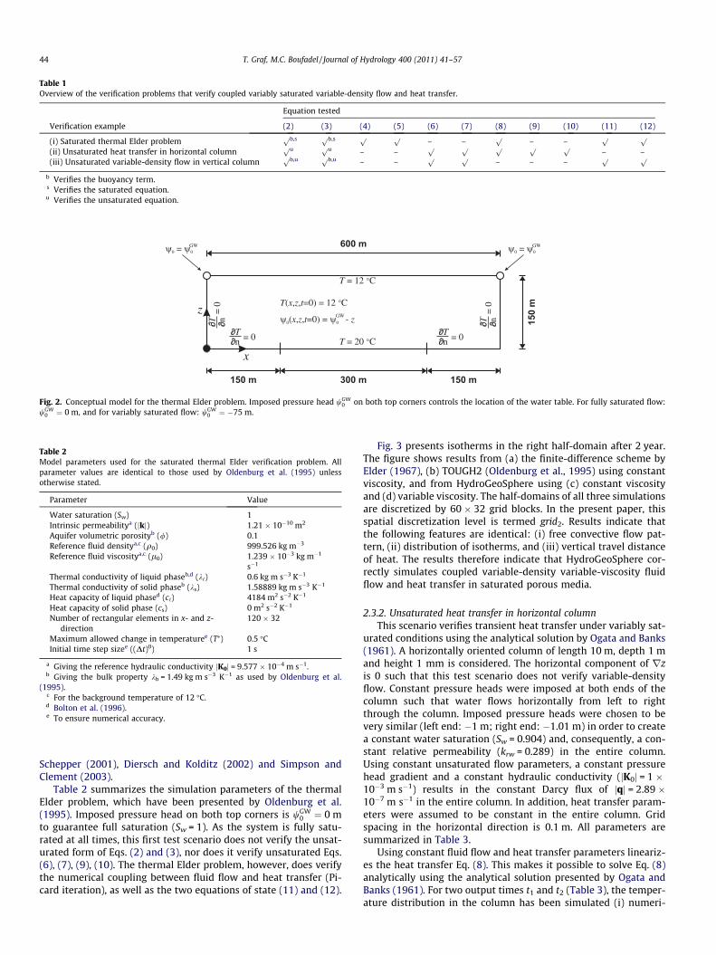
Table 1Overview of the verification problems that verify coupled variably saturated variable-density flow and heat transfer.

Equation tested

Verification example (2) (3) (4) (5) (6) (7) (8) (9) (10) (11) (12)

(i) Saturated thermal Elder problempb,s pb,s p p

– –p

– –p p

(ii) Unsaturated heat transfer in horizontal columnpu pu – –

p p p p p– –

(iii) Unsaturated variable-density flow in vertical columnpb,u pb,u – –

p p– – –

p p

b Verifies the buoyancy term.s Verifies the saturated equation.u Verifies the unsaturated equation.

600 m

150

mT x z t( , , =0) = 12 C°

0( , , =0) = -x z t z0

300 m 150 m150 m

x

z

T = 12 C°

T = 20 C°Tn = 0T

n = 0

T n0

=

T n0

=

0 = 0 0 = 0GW GW

GW

Fig. 2. Conceptual model for the thermal Elder problem. Imposed pressure head wGW0 on both top corners controls the location of the water table. For fully saturated flow:

wGW0 ¼ 0 m, and for variably saturated flow: wGW

0 ¼ �75 m.

Table 2Model parameters used for the saturated thermal Elder verification problem. Allparameter values are identical to those used by Oldenburg et al. (1995) unlessotherwise stated.

Parameter Value

Water saturation (Sw) 1Intrinsic permeabilitya (jkj) 1.21 � 10�10 m2

Aquifer volumetric porosityb (/) 0.1Reference fluid densitya,c (q0) 999.526 kg m�3

Reference fluid viscositya,c (l0) 1.239 � 10�3 kg m�1

s�1

Thermal conductivity of liquid phaseb,d (k‘) 0.6 kg m s�3 K�1

Thermal conductivity of solid phaseb (ks) 1.58889 kg m s�3 K�1

Heat capacity of liquid phased (c‘) 4184 m2 s�2 K�1

Heat capacity of solid phase (cs) 0 m2 s�2 K�1

Number of rectangular elements in x- and z-direction

120 � 32

Maximum allowed change in temperaturee (T⁄) 0.5 �CInitial time step sizee ((Dt)0) 1 s

a Giving the reference hydraulic conductivity jK0j = 9.577 � 10�4 m s�1.b Giving the bulk property kb = 1.49 kg m s�3 K�1 as used by Oldenburg et al.

(1995).c For the background temperature of 12 �C.d Bolton et al. (1996).e To ensure numerical accuracy.


Schepper (2001), Diersch and Kolditz (2002) and Simpson andClement (2003).

Table 2 summarizes the simulation parameters of the thermalElder problem, which have been presented by Oldenburg et al.(1995). Imposed pressure head on both top corners is wGW

0 ¼ 0 mto guarantee full saturation (Sw = 1). As the system is fully satu-rated at all times, this first test scenario does not verify the unsat-urated form of Eqs. (2) and (3), nor does it verify unsaturated Eqs.(6), (7), (9), (10). The thermal Elder problem, however, does verifythe numerical coupling between fluid flow and heat transfer (Pi-card iteration), as well as the two equations of state (11) and (12).

Fig. 3 presents isotherms in the right half-domain after 2 year.The figure shows results from (a) the finite-difference scheme byElder (1967), (b) TOUGH2 (Oldenburg et al., 1995) using constantviscosity, and from HydroGeoSphere using (c) constant viscosityand (d) variable viscosity. The half-domains of all three simulationsare discretized by 60 � 32 grid blocks. In the present paper, thisspatial discretization level is termed grid2. Results indicate thatthe following features are identical: (i) free convective flow pat-tern, (ii) distribution of isotherms, and (iii) vertical travel distanceof heat. The results therefore indicate that HydroGeoSphere cor-rectly simulates coupled variable-density variable-viscosity fluidflow and heat transfer in saturated porous media.

2.3.2. Unsaturated heat transfer in horizontal columnThis scenario verifies transient heat transfer under variably sat-

urated conditions using the analytical solution by Ogata and Banks(1961). A horizontally oriented column of length 10 m, depth 1 mand height 1 mm is considered. The horizontal component of rzis 0 such that this test scenario does not verify variable-densityflow. Constant pressure heads were imposed at both ends of thecolumn such that water flows horizontally from left to rightthrough the column. Imposed pressure heads were chosen to bevery similar (left end: �1 m; right end: �1.01 m) in order to createa constant water saturation (Sw = 0.904) and, consequently, a con-stant relative permeability (krw = 0.289) in the entire column.Using constant unsaturated flow parameters, a constant pressurehead gradient and a constant hydraulic conductivity (jK0j = 1 �10�3 m s�1) results in the constant Darcy flux of jqj = 2.89 �10�7 m s�1 in the entire column. In addition, heat transfer param-eters were assumed to be constant in the entire column. Gridspacing in the horizontal direction is 0.1 m. All parameters aresummarized in Table 3.

Using constant fluid flow and heat transfer parameters lineariz-es the heat transfer Eq. (8). This makes it possible to solve Eq. (8)analytically using the analytical solution presented by Ogata andBanks (1961). For two output times t1 and t2 (Table 3), the temper-ature distribution in the column has been simulated (i) numeri-

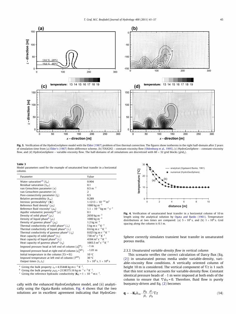
Fig. 3. Verification of the HydroGeoSphere model with the Elder (1967) problem of free thermal convection. The figures show isotherms in the right half-domain after 2 yearsof simulation time from (a) Elder’s (1967) finite-difference scheme, (b) TOUGH2 – constant-viscosity flow (Oldenburg et al., 1995), (c) HydroGeoSphere – constant-viscosityflow, and (d) HydroGeoSphere – variable-viscosity flow. The half-domains of all simulations are discretized with 60 � 32 grid blocks (grid2).

Table 3Model parameters used for the example of unsaturated heat transfer in a horizontalcolumn.

Parameter Value

Water saturationa,b (Sw) 0.904Residual saturation (Swr) 0.1van Genuchten parameter (a) 0.5 m�1

van Genuchten parameter (n) 2Pore-connectivity parameter (lp) 0.5Relative permeability (krw) 0.289Intrinsic permeabilityc (jkj) 1.1213 � 10�10 m2

Reference fluid densityc (q0) 1000 kg m�3

Reference fluid viscosityc (l0) 1.1 � 10�3 kg m�1 s�1

Aquifer volumetric porositya,b (/) 0.1Density of solid phaseb (qs) 2650 kg m�3

Density of liquid phaseb (q‘) 1000 kg m�3

Density of gaseous phaseb (qg) 1.2 kg m�3

Thermal conductivity of solid phasea (ks) 5 kg m s�3 K�1

Thermal conductivity of liquid phasea (k‘) 0.6 kg m s�3 K�1

Thermal conductivity of gaseous phasea (kg) 0.025 kg m s�3 K�1

Heat capacity of solid phaseb (cs) 738 m2 s�2 K�1

Heat capacity of liquid phaseb (c‘) 4184 m2 s�2 K�1

Heat capacity of gaseous phaseb (cg) 1003.5 m2 s�2 K�1

Imposed pressure head at left end of column (wleft0 ) �1 m

Imposed pressure head at right end of column (wright0 ) �1.01 m

Initial temperature in the column (T(t = 0)) 10 �CImposed temperature at left end of column (Tleft) 30 �COutput times (t1, t2) 5 � 105 s, 1 � 106 s

a Giving the bulk property kb = 4.55448 kg m s�3 K�1.b Giving the bulk property qbcb = 2138375.16 kg m�1 s�2 K�1.c Giving the reference hydraulic conductivity jK0j = 1 � 10�3 m s�1.

0

10

20

30

0 2 4 6 8 10

distance [m]

tem

pera

ture

[°C

] analytical (Ogataand Banks, 1961)

numerical (HydroGeoSphere)

(a) (b)

Fig. 4. Verification of unsaturated heat transfer in a horizontal column of 10 mlength using the analytical solution by Ogata and Banks (1961). Temperaturedistributions at two times are compared: (a) 5 � 105 s, and (b) 1 � 106 s. Gridspacing along the column is 0.1 m.


cally with the enhanced HydroGeoSphere model, and (ii) analyti-cally using the Ogata-Banks solution. Fig. 4 shows that the twosolutions are in excellent agreement indicating that HydroGeo-

Sphere correctly simulates transient heat transfer in unsaturatedporous media.

2.3.3. Unsaturated variable-density flow in vertical columnThis scenario verifies the correct calculation of Darcy flux (Eq.

(2)) in unsaturated porous media under variable-density, vari-able-viscosity flow conditions. A vertically oriented column ofheight 10 m is considered. The vertical component of rz is 1 suchthat this test scenario accounts for variable-density flow. Constantidentical pressure heads of �1 m were imposed at both ends of thecolumn to ensure that rw0 = 0. Therefore, fluid flow is purelybuoyancy-driven and Eq. (2) becomes

q ¼ �K0krw �l0

l‘

� q‘

q0rz ð14Þ

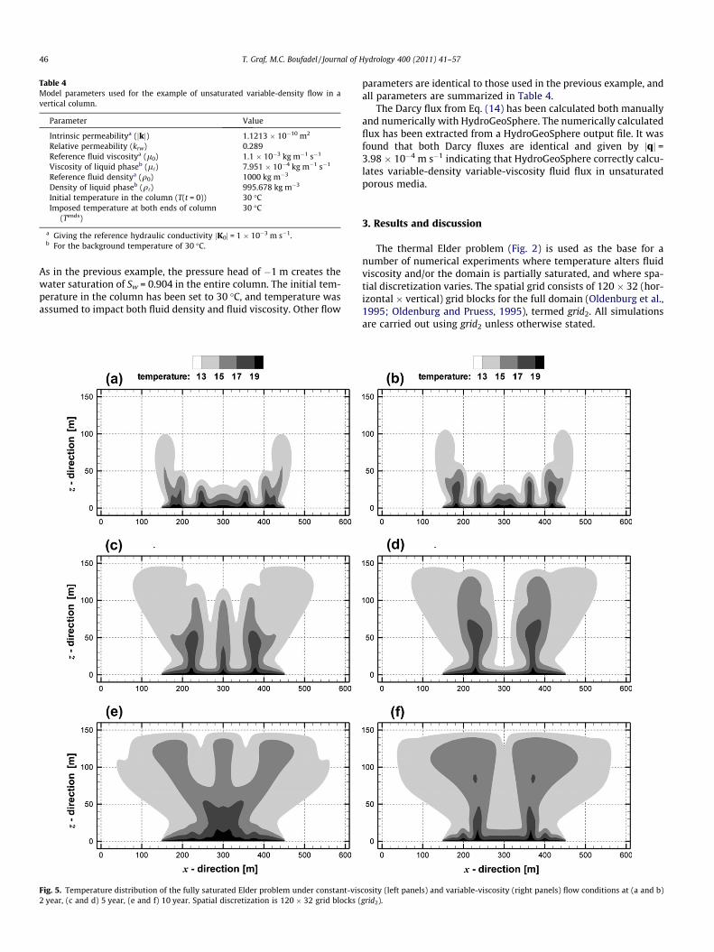
Table 4Model parameters used for the example of unsaturated variable-density flow in avertical column.

Parameter Value

Intrinsic permeabilitya (jkj) 1.1213 � 10�10 m2

Relative permeability (krw) 0.289Reference fluid viscositya (l0) 1.1 � 10�3 kg m�1 s�1

Viscosity of liquid phaseb (l‘) 7.951 � 10�4 kg m�1 s�1

Reference fluid densitya (q0) 1000 kg m�3

Density of liquid phaseb (q‘) 995.678 kg m�3

Initial temperature in the column (T(t = 0)) 30 �CImposed temperature at both ends of column

(Tends)30 �C

a Giving the reference hydraulic conductivity jK0j = 1 � 10�3 m s�1.b For the background temperature of 30 �C.


As in the previous example, the pressure head of �1 m creates thewater saturation of Sw = 0.904 in the entire column. The initial tem-perature in the column has been set to 30 �C, and temperature wasassumed to impact both fluid density and fluid viscosity. Other flow

Fig. 5. Temperature distribution of the fully saturated Elder problem under constant-vis2 year, (c and d) 5 year, (e and f) 10 year. Spatial discretization is 120 � 32 grid blocks (

parameters are identical to those used in the previous example, andall parameters are summarized in Table 4.

The Darcy flux from Eq. (14) has been calculated both manuallyand numerically with HydroGeoSphere. The numerically calculatedflux has been extracted from a HydroGeoSphere output file. It wasfound that both Darcy fluxes are identical and given by jqj =3.98 � 10�4 m s�1 indicating that HydroGeoSphere correctly calcu-lates variable-density variable-viscosity fluid flux in unsaturatedporous media.

3. Results and discussion

The thermal Elder problem (Fig. 2) is used as the base for anumber of numerical experiments where temperature alters fluidviscosity and/or the domain is partially saturated, and where spa-tial discretization varies. The spatial grid consists of 120 � 32 (hor-izontal � vertical) grid blocks for the full domain (Oldenburg et al.,1995; Oldenburg and Pruess, 1995), termed grid2. All simulationsare carried out using grid2 unless otherwise stated.

cosity (left panels) and variable-viscosity (right panels) flow conditions at (a and b)grid2).


For simplicity, we assumed the domain to be homogeneous,which is a common assumption of the reservoir-scale Elder prob-lem. While homogeneity of a reservoir-scale problem may not berealistic, we neglected heterogeneity in order to keep the level ofcomplexity of our conceptual model low. However, in a modelingstudy, Prasad and Simmons (2003) have shown that heterogeneityis a key factor controlling variable-density flow on the reservoirscale. The effect of heterogeneity should therefore be accountedfor in a future study.

Convergence of the unsaturated flow solution occurs when (i)the number of Newton iterations is smaller than 25, and (ii) themaximum absolute nodal change in pressure head over the domainfor one Newton iteration is less than the absolute convergence tol-erance of 10�5 m. Convergence of the variable-density flow solu-tion occurs when (i) the number of Picard iterations is smallerthan 100, and (ii) the maximum relative nodal change in pressurehead and temperature over the domain for one Picard iteration isless than 1%.

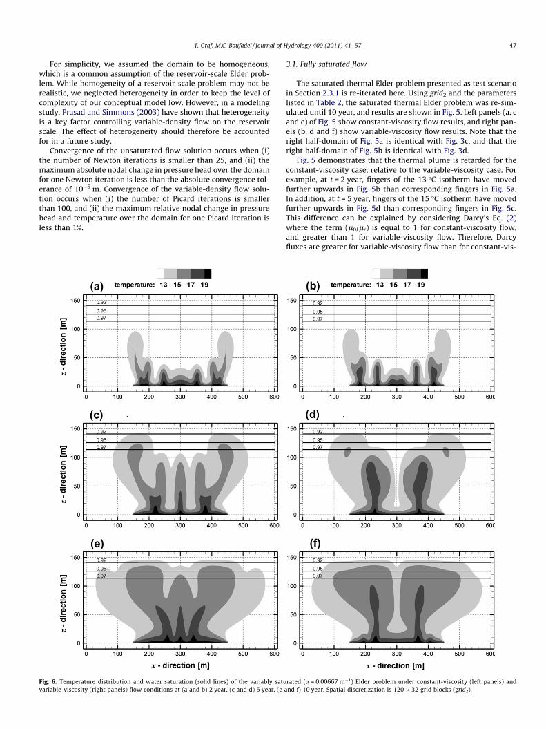
Fig. 6. Temperature distribution and water saturation (solid lines) of the variably satuvariable-viscosity (right panels) flow conditions at (a and b) 2 year, (c and d) 5 year, (e

3.1. Fully saturated flow

The saturated thermal Elder problem presented as test scenarioin Section 2.3.1 is re-iterated here. Using grid2 and the parameterslisted in Table 2, the saturated thermal Elder problem was re-sim-ulated until 10 year, and results are shown in Fig. 5. Left panels (a, cand e) of Fig. 5 show constant-viscosity flow results, and right pan-els (b, d and f) show variable-viscosity flow results. Note that theright half-domain of Fig. 5a is identical with Fig. 3c, and that theright half-domain of Fig. 5b is identical with Fig. 3d.

Fig. 5 demonstrates that the thermal plume is retarded for theconstant-viscosity case, relative to the variable-viscosity case. Forexample, at t = 2 year, fingers of the 13 �C isotherm have movedfurther upwards in Fig. 5b than corresponding fingers in Fig. 5a.In addition, at t = 5 year, fingers of the 15 �C isotherm have movedfurther upwards in Fig. 5d than corresponding fingers in Fig. 5c.This difference can be explained by considering Darcy’s Eq. (2)where the term (l0/l‘) is equal to 1 for constant-viscosity flow,and greater than 1 for variable-viscosity flow. Therefore, Darcyfluxes are greater for variable-viscosity flow than for constant-vis-

rated (a = 0.00667 m�1) Elder problem under constant-viscosity (left panels) andand f) 10 year. Spatial discretization is 120 � 32 grid blocks (grid2).


cosity flow. This is evidenced by the faster movement of the ther-mal front in Fig. 5b, relative to the thermal front in Fig. 5a. Thisobservation is similar to previous findings of viscosity-dependentDarcy flux in solutal variable-density flow problems (e.g. Forkeland Celia, 1992; Boufadel et al., 1999b). For solutal (salt) flow,however, viscosity variations decrease water flux, which is due tothe increase of viscosity with increasing solute concentration.

Viscosity also significantly modifies the convective pattern andthe temperature distribution. Clearly, constant-viscosity flow pro-duces central upwelling (at x = 300 m), whereas variable-viscosityflow produces central downwelling. This effect can be best ob-served after 5 yr (Fig. 5c and d), where one central finger (threethermal fingers in total) forms for constant-viscosity flow, and nocentral finger (two thermal fingers in total) forms for variable-vis-cosity flow. Interestingly, Boufadel et al. (1999b) have observed theopposite for solutal variable-density flow, where no central fingerforms for constant-viscosity flow, and one central finger formsfor variable-viscosity flow. However, the central flow direction is

Fig. 7. Temperature distribution and water saturation (solid lines) of the variably satvariable-viscosity (right panels) flow conditions at (a and b) 2 year, (c and d) 5 year, (e

identical for both constant-viscosity cases (thermal and solutal)and for both variable-viscosity cases (thermal and solutal) becausehigh temperature is imposed at the bottom of the domain (for thethermal Elder problem) and high concentration is imposed at thetop of the domain (for the solutal Elder problem).

It can be concluded that, if saturated flow conditions areencountered in a deep sedimentary basin or a geothermal reser-voir, temperature-dependent viscosity effects are significant inthe flow dynamics, and can not be neglected. This finding contraststo solutal variable-density flow where viscosity does not seem toplay an important role at low concentration, for example at seawa-ter salinity (Boufadel, 2000).

3.2. Variably saturated flow

To allow for variably saturated flow, imposed pressure head onboth top corners is wGW

0 ¼ �75 m, which puts the water table atz = 75 m (Boufadel et al., 1999b). In accordance with Boufadel

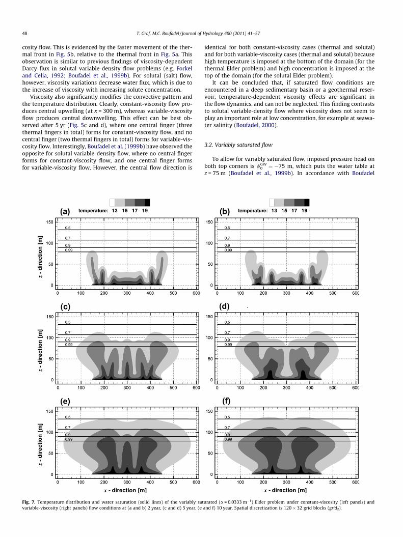
urated (a = 0.0333 m�1) Elder problem under constant-viscosity (left panels) andand f) 10 year. Spatial discretization is 120 � 32 grid blocks (grid2).


et al. (1999b), the van Genuchten parameter n is 2, residual satura-tion Srw is 0.06, pore-connectivity parameter lp is 0.5, and two soiltypes are considered: (i) a fine-textured soil with a = 0.00667 m�1

creating high soil moisture at the soil surface, and (ii) a coarse-textured soil with a = 0.0333 m�1 creating low soil moisture atthe soil surface. The fully saturated case presented in Section 3.1,and the two variably saturated cases presented in this Section3.2 therefore represent a series of cases where the soil saturationcontinuously decreases. Note that the inverse of the a value repre-sents the thickness of the capillary fringe (Boufadel et al., 1999b).Thus, the capillary fringe has a theoretical thickness of 150 m forthe fine-textured soil and 30 m for the coarse-textured soil. Theseemingly unrealistical values for a and the capillary fringe stemfrom the fact that the reservoir-scale (600 m � 150 m) Elderproblem regarded here is an upscaled version of the original labo-ratory-scale (20 cm � 5 cm) Elder problem. Projected back to theoriginal laboratory-scale, the capillary fringe for both soil types is5 cm for the fine-textured soil and 1 cm for the coarse-texturedsoil. However, for consistency and since the focus of this study is

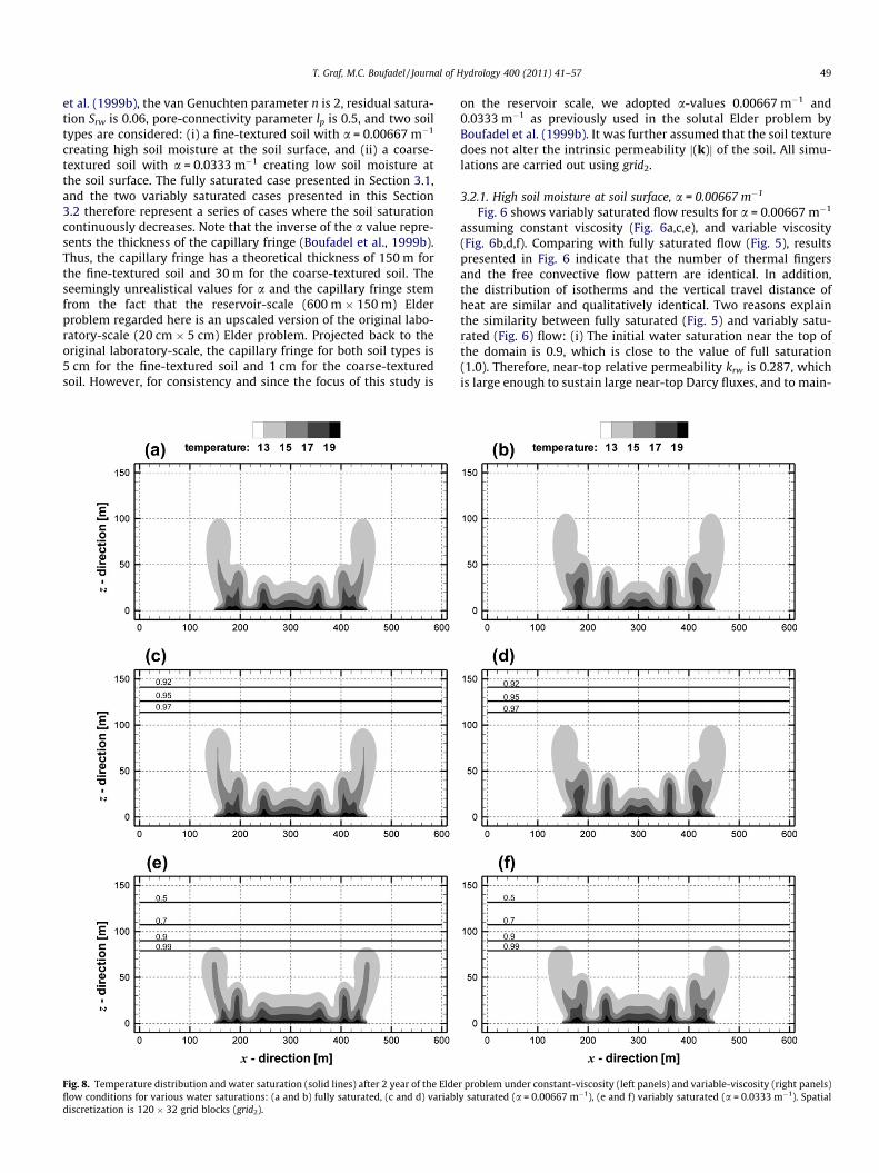
Fig. 8. Temperature distribution and water saturation (solid lines) after 2 year of the Eldeflow conditions for various water saturations: (a and b) fully saturated, (c and d) variabldiscretization is 120 � 32 grid blocks (grid2).

on the reservoir scale, we adopted a-values 0.00667 m�1 and0.0333 m�1 as previously used in the solutal Elder problem byBoufadel et al. (1999b). It was further assumed that the soil texturedoes not alter the intrinsic permeability j(k)j of the soil. All simu-lations are carried out using grid2.

3.2.1. High soil moisture at soil surface, a = 0.00667 m�1

Fig. 6 shows variably saturated flow results for a = 0.00667 m�1

assuming constant viscosity (Fig. 6a,c,e), and variable viscosity(Fig. 6b,d,f). Comparing with fully saturated flow (Fig. 5), resultspresented in Fig. 6 indicate that the number of thermal fingersand the free convective flow pattern are identical. In addition,the distribution of isotherms and the vertical travel distance ofheat are similar and qualitatively identical. Two reasons explainthe similarity between fully saturated (Fig. 5) and variably satu-rated (Fig. 6) flow: (i) The initial water saturation near the top ofthe domain is 0.9, which is close to the value of full saturation(1.0). Therefore, near-top relative permeability krw is 0.287, whichis large enough to sustain large near-top Darcy fluxes, and to main-

r problem under constant-viscosity (left panels) and variable-viscosity (right panels)y saturated (a = 0.00667 m�1), (e and f) variably saturated (a = 0.0333 m�1). Spatial


tain near-top free convection. (ii) Much of the fluid flow takes placein the lower half of the domain, which is always saturated, even forvariably saturated flow.

Fig. 6 also indicates that the thermal plume is retarded for theconstant-viscosity case, relative to the variable-viscosity case. Anidentical observation was done for fully saturated flow (Fig. 5).Similar to fully saturated flow, the shape of the heat plumes undervariably saturated conditions are different and appear to be con-trolled by the viscosity model. Three thermal fingers (including acentral finger) form for constant-viscosity flow, and two thermalfingers (no central finger) form for variable-viscosity flow.

It can be concluded that for variably saturated flow conditionswith high soil moisture, capillarity plays a minor role in the trans-fer of heat, and can be neglected. Changes of fluid viscosity due totemperature, however, significantly impact flow, and must beaccounted for. This result contrasts with results of variably satu-rated flow of salt, where capillarity for almost-saturated conditionsplays a major role, and where viscosity effects can be neglected(Boufadel et al., 1999b).

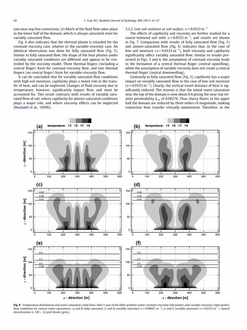
Fig. 9. Temperature distribution and water saturation (solid lines) after 5 year of the Eldeflow conditions for various water saturations: (a and b) fully saturated, (c and d) variabldiscretization is 120 � 32 grid blocks (grid2).

3.2.2. Low soil moisture at soil surface, a = 0.0333 m�1

The effects of capillarity and viscosity are further studied for acoarse-textured soil with a = 0.0333 m�1, and results are shownin Fig. 7. Comparison with results of fully saturated flow (Fig. 5)and almost-saturated flow (Fig. 6) indicates that, in the case oflow soil moisture (a = 0.0333 m�1), both viscosity and capillaritysignificantly affect variably saturated flow. Similar to results pre-sented in Figs. 5 and 6, the assumption of constant viscosity leadsto the formation of a central thermal finger (central upwelling),while the assumption of variable viscosity does not create a centralthermal finger (central downwelling).

Contrarily to fully saturated flow (Fig. 5), capillarity has a majorimpact on variably saturated flow in the case of low soil moisture(a = 0.0333 m�1). Clearly, the vertical travel distance of heat is sig-nificantly reduced. The reasons is that the initial water saturationnear the top of the domain is now about 0.4 giving the near-top rel-ative permeability krw of 0.00276. Thus, Darcy fluxes in the upperhalf the domain are reduced by three orders of magnitude, makingconvective heat transfer virtually nonexistent. Therefore, in the

r problem under constant-viscosity (left panels) and variable-viscosity (right panels)y saturated (a = 0.00667 m�1), (e and f) variably saturated (a = 0.0333 m�1). Spatial


lower half of the domain, heat is transferred by conduction andconvection, while heat transfer in the upper half is limited to con-duction only.

It can be concluded that for variably saturated flow conditionswith low soil moisture, both viscosity and capillarity play a majorrole in the transfer of heat, and must be accounted for.

3.3. Summary of transient results

Results presented in Figs. 5–7 are rearranged to compare the ef-fects of viscosity and capillarity at specific output times. Figs. 8–10present results of fully saturated flow, and variably saturated flowwith high (a = 0.00667 m�1) and low (a = 0.0333 m�1) soil mois-ture at 2 yr, 5 year and 10 year, respectively. Left panels (a, c ande) of the figures show constant-viscosity flow results, and rightpanels (b, d and f) show variable-viscosity flow results. Resultsare arranged in the order of decreasing saturation: (a and b) fullysaturated conditions, (c and d) variably saturated conditions with

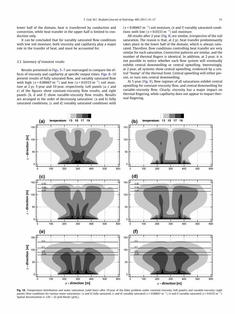
Fig. 10. Temperature distribution and water saturation (solid lines) after 10 year of thepanels) flow conditions for various water saturations: (a and b) fully saturated, (c and d)Spatial discretization is 120 � 32 grid blocks (grid2).

(a = 0.00667 m�1) soil moisture, (e and f) variably saturated condi-tions with low (a = 0.0333 m�1) soil moisture.

All results after 2 year (Fig. 8) are similar, irrespective of the soilsaturation. The reason is that, at 2 yr, heat transfer predominantlytakes place in the lower half of the domain, which is always satu-rated. Therefore, flow conditions controlling heat transfer are verysimilar for each saturation. Convective patterns are similar, and thenumber of thermal fingers is identical. In addition, at 2 year, it isnot possible to notice whether each flow system will eventuallyexhibit central downwelling or central upwelling. Interestingly,at 2 year, all systems show central upwelling, evidenced by a cen-tral ‘‘bump’’ of the thermal front. Central upwelling will either per-sist, or turn into central downwelling.

At 5 year (Fig. 9), flow regimes of all saturations exhibit centralupwelling for constant-viscosity flow, and central downwelling forvariable-viscosity flow. Clearly, viscosity has a major impact onthermal fingering, while capillarity does not appear to impact ther-mal fingering.

Elder problem under constant-viscosity (left panels) and variable-viscosity (rightvariably saturated (a = 0.00667 m�1), (e and f) variably saturated (a = 0.0333 m�1).


Flow phenomena observed at 5 year persist to exist at 10 year(Fig. 10). The central thermal finger (central upwelling) for con-stant-viscosity flow is maintained, and central downwelling is ob-served for variable-viscosity flow for all saturations. Results after10 year clearly show that capillarity remains to have a major im-pact on free convective patterns. The thermal plume for fully satu-rated flow (Fig. 10ab) is transported vertically much further thanthe thermal plume under variably saturated conditions for low soilmoisture (Fig. 10ef). The horizontal extension, however, of the var-iably saturated plume appears to be much larger than the horizon-tal extension of the fully saturated plume. Interestingly, the watertable at z = 75 m acts as a ‘‘lid’’ to flow dynamics, and it appears todivert the thermal plume laterally.

3.4. Spatial discretization

For the solutal Elder problem, several authors have shown thatspatial discretization has a major influence on free convective flowpattern (e.g. Oldenburg and Pruess, 1995; Kolditz et al., 1998;Frolkovic and De Schepper, 2001; Diersch and Kolditz, 2002; Graf

Fig. 11. Temperature distribution after 5 year of the fully saturated Elder problem underfor various spatial discretizations: (a and b) coarse grid1, 72 � 22 grid blocks, (c and d)

and Therrien, 2005; Prasad and Simmons, 2005). Successive gridrefinement indicated that the central flow direction changes asthe grid becomes finer. Locally adaptive grids used by Frolkovicand De Schepper (2001) have been found to generate results iden-tical to those from an extremely fine grid. Therefore, Frolkovic andDe Schepper (2001) have concluded that the result with an adap-tive grid is ‘‘the exact solution of the Elder problem’’. However,the results of the Elder problem at even higher grid levels (finergrids) remain unknown. In addition, grid sensitivity of the originalthermal Elder problem for different viscosity assumptions and cap-illarities still remains unclear.

In this section, the sensitivity of the original thermal Elder prob-lem to spatial discretization is verified. We are not using adaptivegrids. Three spatial grids are considered: (i) a coarse grid with72 � 22 (horizontal � vertical) grid blocks for the full domain,termed grid1, (ii) a medium grid with 120 � 32 grid blocks, termedgrid2, and (iii) a fine grid with 168 � 42 grid blocks, termed grid3. Ina grid refinement study of the solutal Elder problem, Oldenburgand Pruess (1995) have previously used grid2 and grid3 with appli-cation to the solutal Elder problem. Extending the coarsening re-

constant-viscosity (left panels) and variable-viscosity (right panels) flow conditionsmedium grid2, 120 � 32 grid blocks, (e and f) fine grid3, 168 � 42 grid blocks.

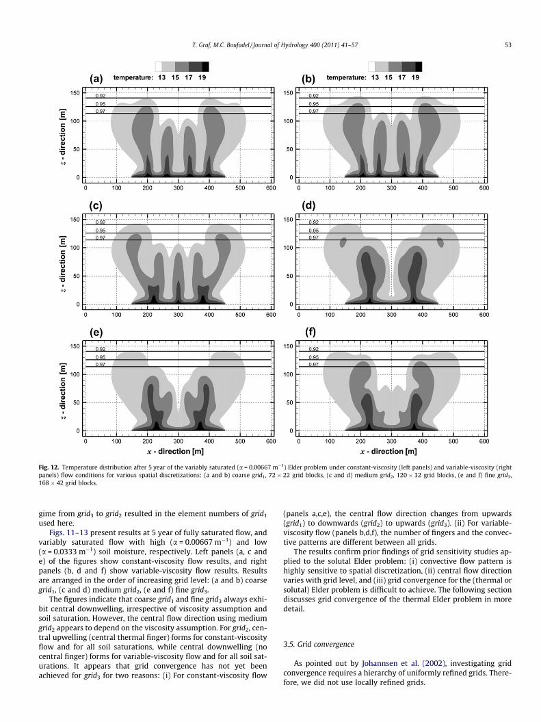
Fig. 12. Temperature distribution after 5 year of the variably saturated (a = 0.00667 m�1) Elder problem under constant-viscosity (left panels) and variable-viscosity (rightpanels) flow conditions for various spatial discretizations: (a and b) coarse grid1, 72 � 22 grid blocks, (c and d) medium grid2, 120 � 32 grid blocks, (e and f) fine grid3,168 � 42 grid blocks.


gime from grid3 to grid2 resulted in the element numbers of grid1

used here.Figs. 11–13 present results at 5 year of fully saturated flow, and

variably saturated flow with high (a = 0.00667 m�1) and low(a = 0.0333 m�1) soil moisture, respectively. Left panels (a, c ande) of the figures show constant-viscosity flow results, and rightpanels (b, d and f) show variable-viscosity flow results. Resultsare arranged in the order of increasing grid level: (a and b) coarsegrid1, (c and d) medium grid2, (e and f) fine grid3.

The figures indicate that coarse grid1 and fine grid3 always exhi-bit central downwelling, irrespective of viscosity assumption andsoil saturation. However, the central flow direction using mediumgrid2 appears to depend on the viscosity assumption. For grid2, cen-tral upwelling (central thermal finger) forms for constant-viscosityflow and for all soil saturations, while central downwelling (nocentral finger) forms for variable-viscosity flow and for all soil sat-urations. It appears that grid convergence has not yet beenachieved for grid3 for two reasons: (i) For constant-viscosity flow

(panels a,c,e), the central flow direction changes from upwards(grid1) to downwards (grid2) to upwards (grid3). (ii) For variable-viscosity flow (panels b,d,f), the number of fingers and the convec-tive patterns are different between all grids.

The results confirm prior findings of grid sensitivity studies ap-plied to the solutal Elder problem: (i) convective flow pattern ishighly sensitive to spatial discretization, (ii) central flow directionvaries with grid level, and (iii) grid convergence for the (thermal orsolutal) Elder problem is difficult to achieve. The following sectiondiscusses grid convergence of the thermal Elder problem in moredetail.

3.5. Grid convergence

As pointed out by Johannsen et al. (2002), investigating gridconvergence requires a hierarchy of uniformly refined grids. There-fore, we did not use locally refined grids.

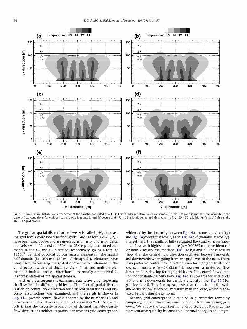
Fig. 13. Temperature distribution after 5 year of the variably saturated (a = 0.0333 m�1) Elder problem under constant-viscosity (left panels) and variable-viscosity (rightpanels) flow conditions for various spatial discretizations: (a and b) coarse grid1, 72 � 22 grid blocks, (c and d) medium grid2, 120 � 32 grid blocks, (e and f) fine grid3,168 � 42 grid blocks.


The grid at spatial discretization level r is called gridr. Increas-ing grid levels correspond to finer grids. Grids at levels r = 1, 2, 3have been used above, and are given by grid1, grid2 and grid3. Gridsat levels r=4. . . 20 consist of 50r and 25r equally distributed ele-ments in the x� and z � direction, respectively, giving a total of1250r2 identical cuboidal porous matrix elements in the spatialhalf-domain (i.e. 300 m � 150 m). Although 3-D elements havebeen used, discretizing the spatial domain with 1 element in they � direction (with unit thickness Dy = 1 m), and multiple ele-ments in both x� and z � directions is essentially a numerical 2-D representation of the spatial domain.

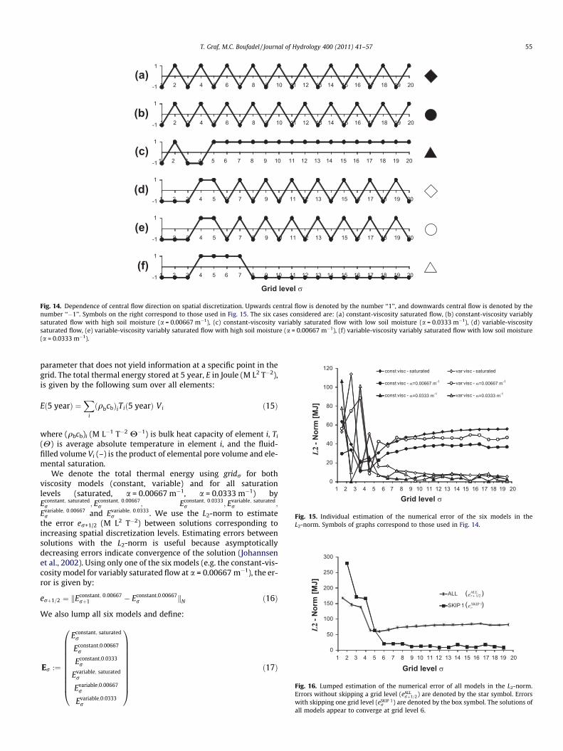
First, grid convergence is examined qualitatively by inspectingthe flow field for different grid levels. The effect of spatial discret-ization on central flow direction for different saturations and vis-cosity assumptions was examined, and the result is shown inFig. 14. Upwards central flow is denoted by the number ‘‘1’’, anddownwards central flow is denoted by the number ‘‘�1’’. A new re-sult is that the viscosity assumption of thermal variable-densityflow simulations neither improves nor worsens grid convergence,

evidenced by the similarity between Fig. 14a–c (constant viscosity)and Fig. 14(constant viscosity) and Fig. 14d–f (variable viscosity).Interestingly, the results of fully saturated flow and variably satu-rated flow with high soil moisture (a = 0.00667 m�1) are identicalfor both viscosity assumptions (Fig. 14a,b,d and e). These resultsshow that the central flow direction oscillates between upwardsand downwards when going from one grid level to the next. Thereis no preferred central flow direction even for high grid levels. Forlow soil moisture (a = 0.0333 m�1), however, a preferred flowdirection does develop for high grid levels. The central flow direc-tion for constant-viscosity flow (Fig. 14c) is upwards for grid levelsP5, and it is downwards for variable-viscosity flow (Fig. 14f) forgrid levels P8. This finding suggests that the solution for vari-able-density flow at low soil moisture may converge, which is ana-lyzed below using the L2-norm.

Second, grid convergence is studied in quantitative terms bycomparing a quantifiable measure obtained from increasing gridlevels. We chose the total thermal energy stored at 5 year as therepresentative quantity because total thermal energy is an integral

Grid level

(a)

(b)

(c)

(d)

(e)

(f)-1

1

-1

1

-1

1

-1

1

-1

1

1

-1 1 2 3 4 5 6 7 8 9 10 11 12 13 14 15 16 17 18 19 20

1 2 3 4 5 6 7 8 9 10 11 12 13 14 15 16 17 18 19 20

1 2 3 4 5 6 7 8 9 10 11 12 13 14 15 16 17 18 19 20

1 2 3 4 5 6 7 8 9 10 11 12 13 14 15 16 17 18 19 20

1 2 3 4 5 6 7 8 9 10 11 12 13 14 15 16 17 18 19 20

1 2 3 4 5 6 7 8 9 10 11 12 13 14 15 16 17 18 19 20

Fig. 14. Dependence of central flow direction on spatial discretization. Upwards central flow is denoted by the number ‘‘1’’, and downwards central flow is denoted by thenumber ‘‘�1’’. Symbols on the right correspond to those used in Fig. 15. The six cases considered are: (a) constant-viscosity saturated flow, (b) constant-viscosity variablysaturated flow with high soil moisture (a = 0.00667 m�1), (c) constant-viscosity variably saturated flow with low soil moisture (a = 0.0333 m�1), (d) variable-viscositysaturated flow, (e) variable-viscosity variably saturated flow with high soil moisture (a = 0.00667 m�1), (f) variable-viscosity variably saturated flow with low soil moisture(a = 0.0333 m�1).

Grid level

L2

]JM[

mroN-

0

20

40

60

80

100

120

1 2 3 4 5 6 7 8 9 10 11 12 13 14 15 16 17 18 19 20

const visc - saturated var visc - saturated

const visc - a=0.00667 var visc - a=0.00667 m-

const visc - a=0.0333 m-1 var visc - a=0.0333 m-1

=0.00667 m-1 =0.00667 m-1

=0.0333 m-1 =0.0333 m-1

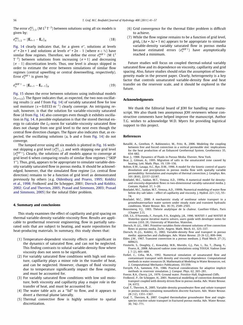
Fig. 15. Individual estimation of the numerical error of the six models in theL2-norm. Symbols of graphs correspond to those used in Fig. 14.

Grid level

L2

]JM[

mroN-

0

50

100

150

200

250

300

1 2 3 4 5 6 7 8 9 10 11 12 13 14 15 16 17 18 19 20

ALL

SKIP 1

( )( )

ALL

SKIP

+ 1/2e

1e

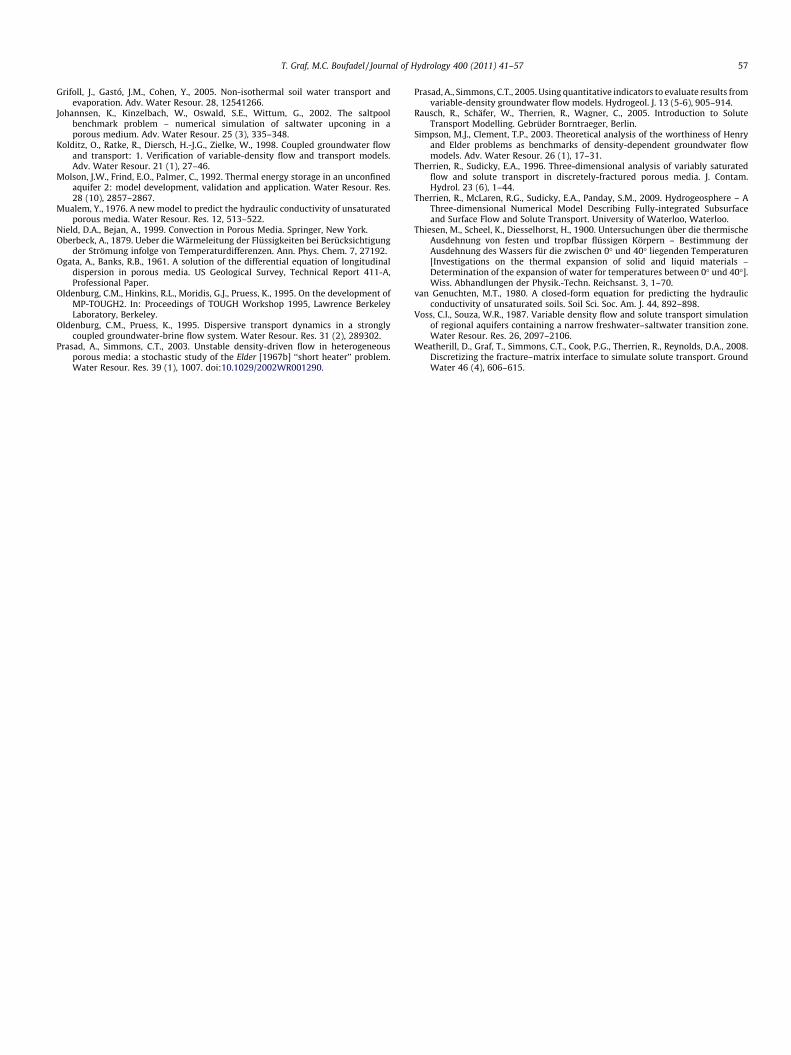
Fig. 16. Lumped estimation of the numerical error of all models in the L2-norm.Errors without skipping a grid level (eALL

rþ1=2) are denoted by the star symbol. Errorswith skipping one grid level (eSKIP 1

r ) are denoted by the box symbol. The solutions of


parameter that does not yield information at a specific point in thegrid. The total thermal energy stored at 5 year, E in Joule (M L2 T�2),is given by the following sum over all elements:

Eð5 yearÞ ¼X

i

ðqbcbÞiTið5 yearÞ Vi ð15Þ

where (qbcb)i (M L�1 T�2 H�1) is bulk heat capacity of element i, Ti

(H) is average absolute temperature in element i, and the fluid-filled volume Vi (–) is the product of elemental pore volume and ele-mental saturation.

We denote the total thermal energy using gridr for bothviscosity models (constant, variable) and for all saturationlevels (saturated, a = 0.00667 m�1, a = 0.0333 m�1) byEconstant; saturated

r ; Econstant; 0:00667r ; Econstant; 0:0333

r ; Evariable; saturatedr ;

Evariable; 0:00667r and Evariable; 0:0333

r . We use the L2-norm to estimatethe error er+1/2 (M L2 T�2) between solutions corresponding toincreasing spatial discretization levels. Estimating errors betweensolutions with the L2-norm is useful because asymptoticallydecreasing errors indicate convergence of the solution (Johannsenet al., 2002). Using only one of the six models (e.g. the constant-vis-cosity model for variably saturated flow at a = 0.00667 m�1), the er-ror is given by:

erþ1=2 ¼ kEconstant; 0:00667rþ1 � Econstant;0:00667

r kN ð16Þ

We also lump all six models and define:

Er :¼

Econstant; saturatedr

Econstant;0:00667r

Econstant;0:0333r

Evariable; saturatedr

Evariable;0:00667r

Evariable;0:0333r

0BBBBBBBBBB@

1CCCCCCCCCCA

ð17Þ

all models appear to converge at grid level 6.


The error eALLrþ1=2 (M L2 T�2) between solutions using all six models is

given by:

eALLrþ1=2 ¼ kErþ1 � ErkN ð18Þ

Fig. 14 clearly indicates that, for a given r⁄, solutions at levelsr⁄ + 2n + 1 and solutions at levels r⁄ + 2n � 1 (where n 2 N) havesimilar flow regimes. Therefore, we define the error eSKIP 1

r (M L2

T�2) between solutions from increasing (r + 1) and decreasing(r � 1) discretization levels. Thus, one level is always skipped inorder to estimate the error between simulations of similar flowregimes (central upwelling or central downwelling, respectively).Error eSKIP 1

r is given by:

eSKIP 1r ¼ kErþ1 � Er�1kN ð19Þ

Fig. 15 shows the error between solutions using individual models(er+1/2). The figure indicates that, as expected, the two non-oscillat-ing results (c and f from Fig. 14) of variably saturated flow for lowsoil moisture (a = 0.0333 m�1) clearly converge. An intriguing re-sult, however, is that the solution for variable-viscosity saturatedflow (d from Fig. 14) also converges even though it exhibits oscilla-tion in Fig. 14. A possible explanation is that the stored thermal en-ergy to calculate the L2-norm for variable-viscosity saturated flowdoes not change from one grid level to the next even though thecentral flow direction changes. The figure also indicates that, as ex-pected, the oscillating solutions (a, b and e from Fig. 14) do notconverge.

The lumped error using all six models is plotted in Fig. 16 with-out skipping a grid level (eALL

rþ1=2), and with skipping one grid level(eSKIP 1

r ). Clearly, the solutions of all models appear to converge atgrid level 6 when comparing results of similar flow regimes (‘‘SKIP1’’). Thus, grid6 appears to be appropriate to simulate variable-den-sity variably saturated flow in porous media. It should be acknowl-edged, however, that the simulated flow regime (i.e. central flowdirection) remains to be a function of grid level as demonstratedpreviously by others (e.g. Oldenburg and Pruess, 1995; Kolditzet al., 1998; Frolkovic and De Schepper, 2001; Diersch and Kolditz,2002; Graf and Therrien, 2005; Prasad and Simmons, 2003; Prasadand Simmons, 2005) for the solutal Elder problem.

4. Summary and conclusions

This study examines the effect of capillarity and grid spacing onthermal variable-density variable-viscosity flow. Results are appli-cable to geothermal reservoir engineering, flow in partially satu-rated soils that are subject to heating, and waste repositories forheat-producing materials. In summary, this study shows that:

(1) Temperature-dependent viscosity effects are significant inthe dynamics of saturated flow, and can not be neglected.This finding contrasts to solutal variable-density flow whereviscosity does not seem to be significant.

(2) For variably saturated flow conditions with high soil mois-ture, capillarity plays a minor role in the transfer of heat,and can be neglected. However, changes of fluid viscositydue to temperature significantly impact the flow regime,and must be accounted for.

(3) For variably saturated flow conditions with low soil mois-ture, both viscosity and capillarity play a major role in thetransfer of heat, and must be accounted for.

(4) The water table acts as a ‘‘lid’’ to flow, and it appears todivert a thermal plume laterally.

(5) Thermal convective flow is highly sensitive to spatialdiscretization.

(6) Grid convergence for the thermal Elder problem is difficultto achieve.

(7) While the flow regime remains to be a function of grid level,grid6 (Dx = Dz = 1 m) appears to be appropriate to simulatevariable-density variably saturated flow in porous mediabecause estimated errors (eSKIP 1

r ) have asymptoticallyreached a minimum.

Future studies will focus on coupled thermal-solutal variablysaturated flow and its dependence on viscosity, capillarity and gridspacing. Also, future studies should relax the assumption of homo-geneity made in the present paper. Clearly, heterogeneity is a keyfactor that controls unsaturated variable-density flow and heattransfer on the reservoir scale, and it should be explored in thefuture.

Acknowledgments

We thank the Editorial board of JOH for handling our manu-script. We also thank two anonymous JOH reviewers whose con-structive comments have helped improve the manuscript. AuthorT.G. wishes to acknowledge W.D. Myers for providing logisticalsupport to this project.

References

Bataillé, A., Genthon, P., Rabinowicz, M., Fritz, B., 2006. Modeling the couplingbetween free and forced convection in a vertical permeable slot: implicationsfor the heat production of an Enhanced Geothermal System. Geothermics 35,654–682.

Bear, J., 1988. Dynamics of Fluids in Porous Media. Elsevier, New York.Bear, J., Gilman, A., 1995. Migration of salts in the unsaturated zone caused by

heating. Lett. Math. Phys. 19, 139–156.Bolton, E.W., Lasaga, A.C., Rye, D.M., 1996. A model for the kinetic control of quartz

dissolution and precipitation in porous media flow with spatially variablepermeability: formulation and examples of thermal convection. J. Geophys. Res.101 (B10), 22157–22187.

Boufadel, M.C., Suidan, M.T., Venosa, A.D., 1999a. A numerical model for density-and-viscosity-dependent flows in two-dimensional variably-saturated media. J.Contam. Hydrol. 37, 1–20.

Boufadel, M.C., Suidan, M.T., Venosa, A.D., 1999b. Numerical modeling of water flowbelow dry salt lakes – effect of capillarity and viscosity. J. Hydrol. 221 (12), 55–74.

Boufadel, M.C., 2000. A mechanistic study of nonlinear solute transport in agroundwatersurface water system under steady state and transient hydraulicconditions. Water Resour. Res. 36 (9), 2549–2565.

Boussinesq, V.J., 1903. Théorie analytique de la chaleur. Gauthier-Villars, Paris(Chapter 2.3).

Clift, S.S., D’Azevedo, F., Forsyth, P.A., Knightly, J.R., 1996. WATSIT-1 and WATSIT-BWaterloo sparse iterative matrix solvers, users guide with developer notes forversion 2.0.0, (8). University of Waterloo, Waterloo.

Diersch, H.-J.G., 1981. Primitive variables finite element solutions of free convectionflows in porous media. Zschr. Angew. Math. Mech. 61, 325–337.

Diersch, H.-J.G., Kolditz, O., 2002. Variable-density flow and transport in porousmedia: approaches and challenges. Adv. Water Resour. 25 (8-12), 899–944.

Elder, J.W., 1967. Transient convection in a porous medium. J. Fluid Mech. 27 (3),609623.

Finsterle, S., Doughty, C., Kowalsky, M.B., Moridis, G.J., Pan, L., Xu, T., Zhang, Y.,Pruess, K., 2008. Advanced vadose zone simulations using TOUGH. Vadose ZoneJ. 7 (2), 601–609.

Forkel, C., Celia, M.A., 1992. Numerical simulation of unsaturated flow andcontaminant transport with density and viscosity dependence. Computationalmethods in water resources IX. Mathematical Modeling in Water Resources, vol.2, Computational Mechanics Publications, 351359.

Forsyth, P.A., Sammon, P.H., 1986. Practical considerations for adaptive implicitmethods in reservoir simulation. J. Comput. Phys. 62, 265–281.

Freeze, R.A., Cherry, J.A., 1979. Ground water. Prentice-Hall, Englewood Cliffs.Frolkovic, P., De Schepper, H., 2001. Numerical modelling of convection dominated

transport coupled with density driven flow in porous media. Adv. Water Resour.24, 6372.

Graf, T., Therrien, R., 2005. Variable-density groundwater flow and solute transportin porous media containing nonuniform discrete fractures. Adv. Water Resour.28 (12), 1351–1367.

Graf, T., Therrien, R., 2007. Coupled thermohaline groundwater flow and single-species reactive solute transport in fractured porous media. Adv. Water Resour.30, 742–771.


Grifoll, J., Gastó, J.M., Cohen, Y., 2005. Non-isothermal soil water transport andevaporation. Adv. Water Resour. 28, 12541266.

Johannsen, K., Kinzelbach, W., Oswald, S.E., Wittum, G., 2002. The saltpoolbenchmark problem – numerical simulation of saltwater upconing in aporous medium. Adv. Water Resour. 25 (3), 335–348.

Kolditz, O., Ratke, R., Diersch, H.-J.G., Zielke, W., 1998. Coupled groundwater flowand transport: 1. Verification of variable-density flow and transport models.Adv. Water Resour. 21 (1), 27–46.

Molson, J.W., Frind, E.O., Palmer, C., 1992. Thermal energy storage in an unconfinedaquifer 2: model development, validation and application. Water Resour. Res.28 (10), 2857–2867.

Mualem, Y., 1976. A new model to predict the hydraulic conductivity of unsaturatedporous media. Water Resour. Res. 12, 513–522.

Nield, D.A., Bejan, A., 1999. Convection in Porous Media. Springer, New York.Oberbeck, A., 1879. Ueber die Wärmeleitung der Flüssigkeiten bei Berücksichtigung

der Strömung infolge von Temperaturdifferenzen. Ann. Phys. Chem. 7, 27192.Ogata, A., Banks, R.B., 1961. A solution of the differential equation of longitudinal

dispersion in porous media. US Geological Survey, Technical Report 411-A,Professional Paper.

Oldenburg, C.M., Hinkins, R.L., Moridis, G.J., Pruess, K., 1995. On the development ofMP-TOUGH2. In: Proceedings of TOUGH Workshop 1995, Lawrence BerkeleyLaboratory, Berkeley.

Oldenburg, C.M., Pruess, K., 1995. Dispersive transport dynamics in a stronglycoupled groundwater-brine flow system. Water Resour. Res. 31 (2), 289302.

Prasad, A., Simmons, C.T., 2003. Unstable density-driven flow in heterogeneousporous media: a stochastic study of the Elder [1967b] ‘‘short heater’’ problem.Water Resour. Res. 39 (1), 1007. doi:10.1029/2002WR001290.

Prasad, A., Simmons, C.T., 2005. Using quantitative indicators to evaluate results fromvariable-density groundwater flow models. Hydrogeol. J. 13 (5-6), 905–914.

Rausch, R., Schäfer, W., Therrien, R., Wagner, C., 2005. Introduction to SoluteTransport Modelling. Gebrüder Borntraeger, Berlin.

Simpson, M.J., Clement, T.P., 2003. Theoretical analysis of the worthiness of Henryand Elder problems as benchmarks of density-dependent groundwater flowmodels. Adv. Water Resour. 26 (1), 17–31.

Therrien, R., Sudicky, E.A., 1996. Three-dimensional analysis of variably saturatedflow and solute transport in discretely-fractured porous media. J. Contam.Hydrol. 23 (6), 1–44.

Therrien, R., McLaren, R.G., Sudicky, E.A., Panday, S.M., 2009. Hydrogeosphere – AThree-dimensional Numerical Model Describing Fully-integrated Subsurfaceand Surface Flow and Solute Transport. University of Waterloo, Waterloo.

Thiesen, M., Scheel, K., Diesselhorst, H., 1900. Untersuchungen über die thermischeAusdehnung von festen und tropfbar flüssigen Körpern – Bestimmung derAusdehnung des Wassers für die zwischen 0� und 40� liegenden Temperaturen[Investigations on the thermal expansion of solid and liquid materials –Determination of the expansion of water for temperatures between 0� und 40�].Wiss. Abhandlungen der Physik.-Techn. Reichsanst. 3, 1–70.

van Genuchten, M.T., 1980. A closed-form equation for predicting the hydraulicconductivity of unsaturated soils. Soil Sci. Soc. Am. J. 44, 892–898.

Voss, C.I., Souza, W.R., 1987. Variable density flow and solute transport simulationof regional aquifers containing a narrow freshwater–saltwater transition zone.Water Resour. Res. 26, 2097–2106.

Weatherill, D., Graf, T., Simmons, C.T., Cook, P.G., Therrien, R., Reynolds, D.A., 2008.Discretizing the fracture–matrix interface to simulate solute transport. GroundWater 46 (4), 606–615.

http://dx.doi.org/10.1029/2002WR001290

Documents

Effect of viscosity, capillarity and grid spacing on thermal variable-density flow