EFFECT OF USING PWM RECTIFIERS AND PHASE

SHIFTED TRANSFORMER FED RECTIFIERS ON

HARMONIC MITIGATION

A THESIS SUBMITTED TO THE GRADUATE

SCHOOL OF APPLIED SCIENCES

OF

NEAR EAST UNIVERSITY

By

SALAR AHMED RASOOL

In Partial Fulfillments of the Requirements For

the Degree of Master of Science

in

Electrical and Electronic Engineering

NICOSIA, 2016

i

I hereby declare that all information in this document has been obtained and presented in

accordance with academic rules and ethical conduct. I also declare that, as required by these

rules and conduct, I have fully cited and referenced all material and results that are not original

to this work.

Name: Salar Ahmed Rasool

Signature:

Date:

ii

ACKNOWLEDGEMENTS

I express my deep appreciation, sincere great thanks and gratitude to my supervisor Assoc.

Prof. Dr. Mehmet Timur Aydemir.

Also I’d like thankful chairman of Department of Electrical and Electronic Engineering Assist.

Prof. Dr. Ali Serener.

Special thanks to my family for their encouragement and more and more patience during the

two years of study.

Finally, I thank Mr. Jabbar Majeed, Mr. Husain Ali, Mr. Abu Bakir Aziz in Erbil technology

institutes, all my friends and those who helped me to complete my study.

iii

To my family…

iv

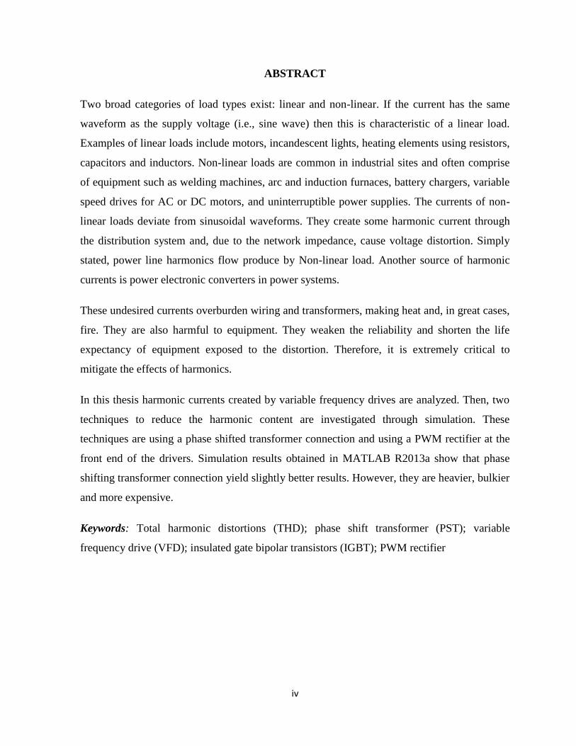
ABSTRACT

Two broad categories of load types exist: linear and non-linear. If the current has the same

waveform as the supply voltage (i.e., sine wave) then this is characteristic of a linear load.

Examples of linear loads include motors, incandescent lights, heating elements using resistors,

capacitors and inductors. Non-linear loads are common in industrial sites and often comprise

of equipment such as welding machines, arc and induction furnaces, battery chargers, variable

speed drives for AC or DC motors, and uninterruptible power supplies. The currents of non-

linear loads deviate from sinusoidal waveforms. They create some harmonic current through

the distribution system and, due to the network impedance, cause voltage distortion. Simply

stated, power line harmonics flow produce by Non-linear load. Another source of harmonic

currents is power electronic converters in power systems.

These undesired currents overburden wiring and transformers, making heat and, in great cases,

fire. They are also harmful to equipment. They weaken the reliability and shorten the life

expectancy of equipment exposed to the distortion. Therefore, it is extremely critical to

mitigate the effects of harmonics.

In this thesis harmonic currents created by variable frequency drives are analyzed. Then, two

techniques to reduce the harmonic content are investigated through simulation. These

techniques are using a phase shifted transformer connection and using a PWM rectifier at the

front end of the drivers. Simulation results obtained in MATLAB R2013a show that phase

shifting transformer connection yield slightly better results. However, they are heavier, bulkier

and more expensive.

Keywords: Total harmonic distortions (THD); phase shift transformer (PST); variable

frequency drive (VFD); insulated gate bipolar transistors (IGBT); PWM rectifier

v

ÖZET

Enerji sistemlerinin yükleri kabaca iki sınıfa ayrılabilir: Doğrusal yükler ve doğrusal olmayan

yükler. Doğrusal yük durumunda yük akımının şekli uygulanan gerilimle aynıdır. Doğrusal

yüklere örnek olarak motorlar, akkor lambalar, rezistive ısıtıcılar, kondansatörler ve

endüktörler gösterilebilir. Öte yandan, sanayide doğrusal olmayan yük kullanımı da yaygındır.

Bunlara örnek olarak da kaynak makineleri, endüksiyon ocakları, ark fırınları, batarya şarj

sistemleri, ayarlanabilir hızlı sürücüler ve kesintisiz güç kaynakları sayılabilir. Doğrusal

olmayan yüklerin akımları bozulmuş sinüs şeklindedir. Bu akımlar dağıtım sistemine

harmonik akımlar enjekte ederler ve şebekenin empedansı nedeniyle gerilim bozuntusuna da

yol açarlar. Basitçe, doğrusal olmayan yüklerin güç sistemlerinde harmonik akım akışına

neden olduğu söylenebilir. Harmonik akımların bir diğer kaynağı da güç elektroniği

devreleridir.

Bu istenmeyen akımlar iletim hatlarının ve transformatörlerin aşırı yüklenmesine neden olurlar

ve ısınmaya, bazı durumlarda da yangına neden olurlar. Ayrıca donanıma da zarar verebilirler.

Bozunum maruz kalan donanımın ömrü kısalır ve güvenilirliği azalır. Bu nedenle,

harmoniklerin etkilerinin azaltılması yaşamsaldır.

Bu tez çalışmasında değişken frekanslı sürücülerin yarattığı harmonikler incelenmekte ve

analiz edilmektedir. Sonra, harmonikleri azaltmak için kullanılan iki yöntem benzetim yoluyla

incelenmektedir. Bu yöntemler faz kaydırıcı transformatör kullanımı ve sürücünün ön katında

PWM doğrultucu kullanımıdır. MATLAB R2013a ile elde edilen benzetim sonuçları faz

kaydırıcı transformatör kullanımının biraz daha iyi sonuç verdiğini göstermektedir. Ancak, bu

sistemler daha ağır, daha hantal ve daha pahalıdır.

Anahtar Kelimeler: Toplam harmonik bozunum; faz kaydırıcı transformatörler; değişken

frekanslı sürücüler; PWM doğrultucu

vi

TABLE OF CONTENTS

AKNOWLEDGMENTS………..………………………………………………………. ii

ABSTRACT…....…………………..……………………………………………………. iv

ÖZET…..………………………………………………………………………….…….... v

TABLE OF CONTENTS…..…….……………………………………………………… vi

LIST OF TABLES……………..………………………………………………………... ix

LIST OF FIGURES…..……………………………………………………………….… x

LIST OF SYMBOLS……..………….…………………………………………………... xiii

LIST OF ABBREVATIONS…...……………………………………………………….. xiv

CHAPTER 1: INTRODUCTION

1.1 Objective………………………………………………..…………………………….. 2

1.2 Thesis Structure…………………………..…………...………………………………. 3

CHAPTER 2: HARMONIC PROBLEM IN POWER SYSTEMS

2.1 Electrical Load Classification…………………...………………………….………… 4

2.1.1 Linear electrical loads….……………………………………………………….. 4

2.1.1.1 Properties of linear loads………..……………...………………………. 5

2.1.2 Non-Linear Electrical Loads…………………………………...……………….. 5

2.1.2.1 Properties of non-linear loads……...…………………………..……….. 6

2.2 Power Factor In Electrical Power Systems…………………………………………… 7

2.2.1 Power factor with linear loads……………………….……….………………… 7

2.2.2 Power factor with non–linear loads and sinusoidal voltage……………....……. 9

2.2.3 Power factor with non–linear loads and voltage distortion…………….……… 11

2.3 Variable Frequency Drives………………………………………………………….... 13

2.4 Harmonics Mitigation………………………………………………………...…...….. 15

2.4.1 Phase displacement of harmonic currents…………………………..….………. 18

2.4.2 Harmonic Cancellation…………………………………………………………. 20

2.5 PWM Rectifier…………………………………………………...………………….... 22

vii

2.5.1 PWM boost type rectifier……………………………………………………...... 22

2.5.2 PWM buck type rectifier……………………………………………...………… 23

CHAPTER 3: PHASE SHIFT TRANSFORMER AND BUCK TYPE PWM

RECTIFIER

3.1 Phase Shift Transformer………………….………………………………………….... 24

3.2 Multi-Pulse Converters…………………..………………………………………….... 25

3.2.1 Bidirectional multi-pulse rectifier….…………………………………………… 26

3.2.2 Unidirectional multi-pulse rectifier….………………………………………….. 26

3.3 Design of (24) Pulse Rectifier…………………………….…………………………... 27

3.3.1 One to four, 3-Ph. system………………………………..……..…………...….. 27

3.3.2 Implementation of rectifier topology………..…………………..……………… 30

3.3.3 Transformers turns ratio……………………………..…………..……………… 31

3.4 Inverter……………………………………...………………………………………… 32

3.5 PWM Buck Rectifier……………….……………..…….…………………………….. 33

CHAPTER 4: SIMULATION, RESULTS AND DISCUSSIONS

4.1 Loading and Driving Motor……………………………………………………….….. 35

4.2 Simulation Model and Results of the Drive with Phase Shift Transformer ………..… 36

4.3 Advantages of 24-Pulse Phase Shift Transformer…….……………………………… 42

4.4 Disadvantages of 24-Pulse Phase Shift Transformer………..………………………... 43

4.5 Simulation Results with Buck Type PWM Rectifier…………………………………. 46

4.6 Properties and Performance of Buck Type PWM Rectifier…………………………... 48

CHAPTER 5: CONCLUSION AND SUGGESTION FOR FUTHURE WORK

5.1 Conclusions ...………………………………………………………………………… 54

5.2 Future Work ...……………...………………………………………………………… 55

REFERENCES……………………………………………………………………….….. 56

viii

APPENDICES

APPENDIX 1: Overall circuit diagram of simulation of 24-pulse phase shift…………... 59

APPENDIX 2: Overall circuit diagram of simulation model of VFD with PWM………. 60

APPENDIX 3: IEEE std 519-1992 harmonic limits………………………………….... 61

ix

LIST OF TABLES

Table 2.1: Some examples of linear loads…………………………..…………….……… 4

Table 2.2: Some examples for non- linear loads………………………….…….……….. 6

Table 3.1: Variation of harmonics and ripple with pulse number…….…..….….….…. 26

Table 4.1: THD, Pf results with varies cases by using phase shift transformer………….. 42

Table 4.2: THD, Pf results with varies cases by using buck type PWM rectifier………... 47

Table 4.3: Comparison of harmonic mitigation methods….……………..……….…...…. 52

Table 4.4: Percentage of harmonics to fundamental………………..……..……………...

53

x

LIST OF FIGURES

Figure 2.1: Characteristics of Linear Loads…………………………………...…..…… 5

Figure 2.2: Characteristics of Non-Linear Loads…………………………….……...… 7

Figure 2.3: Power triangle…………………………………………………………..….. 8

Figure 2.4: Power triangle with capacitor bank…………………………………….….. 8

Figure 2.5: Power triangle in non-linear load and sinusoidal voltage………………..… 11

Figure 2.6: Power triangle in non-linear load and sinusoidal voltage with Capacitor…. 11

Figure 2.7: Power triangle in non-linear load and voltage distortion…………….……. 13

Figure 2.8: Power triangle in non-linear load and voltage distortion With Capacitor…. 14

Figure 2.9: VFD system………………………………………………………………… 15

Figure 2.10: Most popular three-phase harmonic reduction techniques of current…….. 16

Figure 2.11: Phase shifting transformer 24-pulse rectifier………………………….….. 17

Figure 2.12: Investigation of Harmonic Currents In The Primary and Secondary …….. 19

Figure 2.13: An Example Of Harmonic Current Cancellation…………………………. 21

Figure 2.14: PWM Rectifier……………………………………………………………. 22

Figure 2.15: Boost type PWM Rectifier…………………………….………………….. 23

Figure 2.16: Buck type PWM Rectifier………………………………………………… 23

Figure 3.1: 24-Pulse Rectifier………………………………………..…………………. 25

Figure 3.2: Input line Va0b0, Vb0c0 and Vc0a0 at DBI………..…………..………….…... 28

Figure 3.3: Input line Va30b30, Vb30c30 and Vc30a30 at DBII………..……….………….… 28

Figure 3.4: Input line Va15b15, Vb15c15 and Vc15a15 at DBIII…………………………….. 29

Figure 3.5: Input line Va45b45, Vb45c45 and Vc45a45 at DBIV…………………………..... 29

Figure 3.6: Schematic Diagram of proposal phase-shift system…………………..…… 33

Figure 3.7: LC filter…………………………………………………………………..… 33

Figure 3.8: Schematic Diagram of proposal PWM system……………….……….…… 34

Figure 4.1: Simulation model of phase shift transformer………………………………. 37

Figure 4.2: Simulation model Circuit Diagram of Phase shift Transformer system….... 38

Figure 4.3: Voltage input to bridge I………………………….………………...…….... 39

xi

Figure 4.4: Voltage input to bridge II……………………………..……………………. 39

Figure 4.5: Voltage input to bridge III………………………………………………….. 39

Figure 4.6: Voltage input to bridge IV……………………………………………….… 40

Figure 4.7: Output dc voltage in bridge I…………………………………………….… 40

Figure 4.8: Output dc voltage in bridge II………………………………………….….. 40

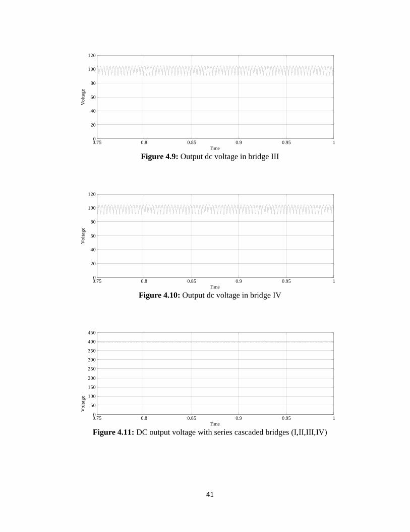
Figure 4.9: Output dc voltage in bridge III…………………………………………..… 41

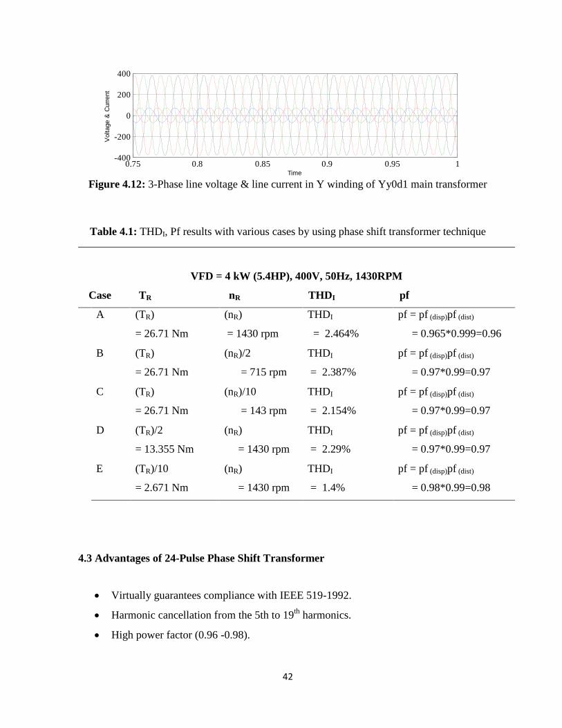
Figure 4.10: Output dc voltage in bridge IV………………………………………….… 41

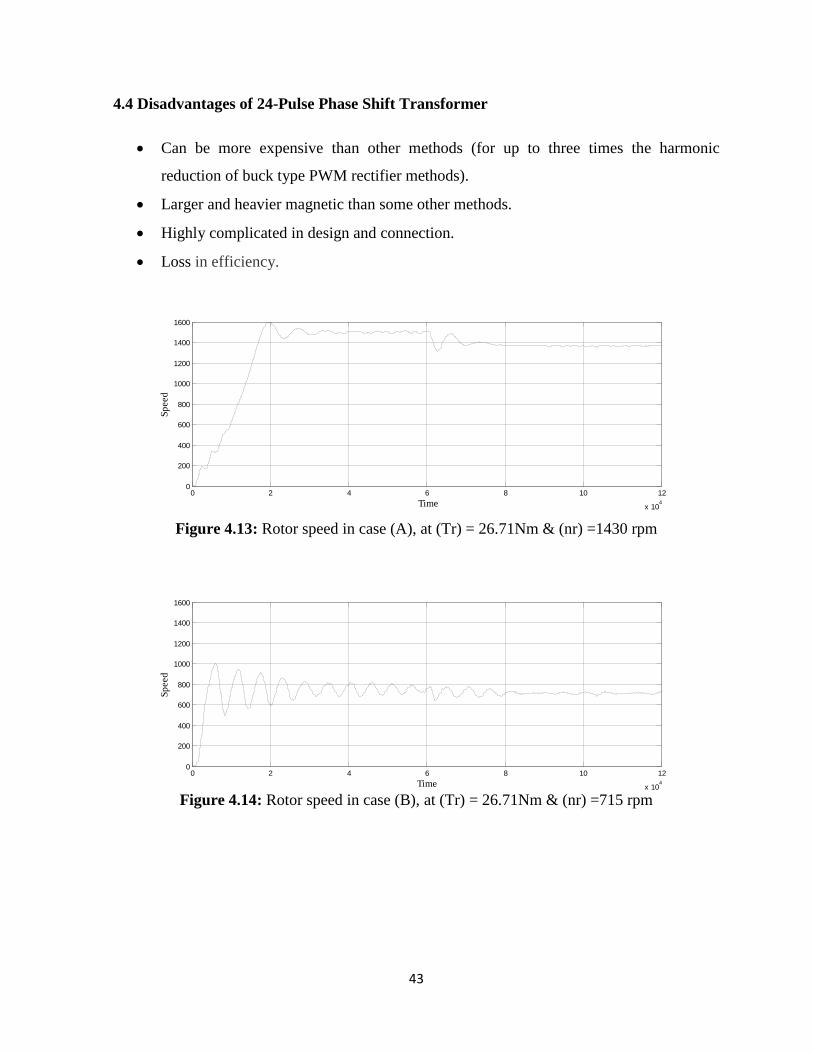
Figure 4.11: DC output voltage with series cascaded bridges (I,II,III,IV)………….…. 41

Figure 4.12: 3-Phase VL & IL in Y Winding of Yy0d1 main Transformer…………...… 42

Figure 4.13: Rotor speed in case (A), At (Tr) = 26.71Nm &(nr) =1430 rpm………….. 43

Figure 4.14: Rotor speed in case (B), At (Tr) = 26.71Nm & (nr) =715 rpm…………… 43

Figure 4.15: Rotor speed in case (C), At (Tr) = 26.71Nm & (nr) =143 rpm…………… 44

Figure 4.16: Rotor speed in case (D), At (Tr) = 13.355Nm & (nr) =1430 rpm………… 44

Figure 4.17: Rotor speed in case (E), At (Tr) = 2.671Nm &(nr) =1430 rpm……….….. 44

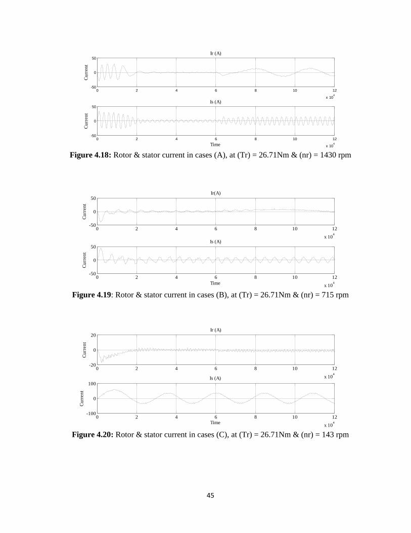
Figure 4.18: Ri & Si in cases (A), At (Tr) = 26.71Nm & (nr) = 1430 rpm……………... 45

Figure 4.19: Ri & Si in cases (B), At (Tr) = 26.71Nm & (nr) = 715 rpm………………. 45

Figure 4.20: Ri & Si in cases (C), At (Tr) = 26.71Nm & (nr) = 143 rpm………………. 45

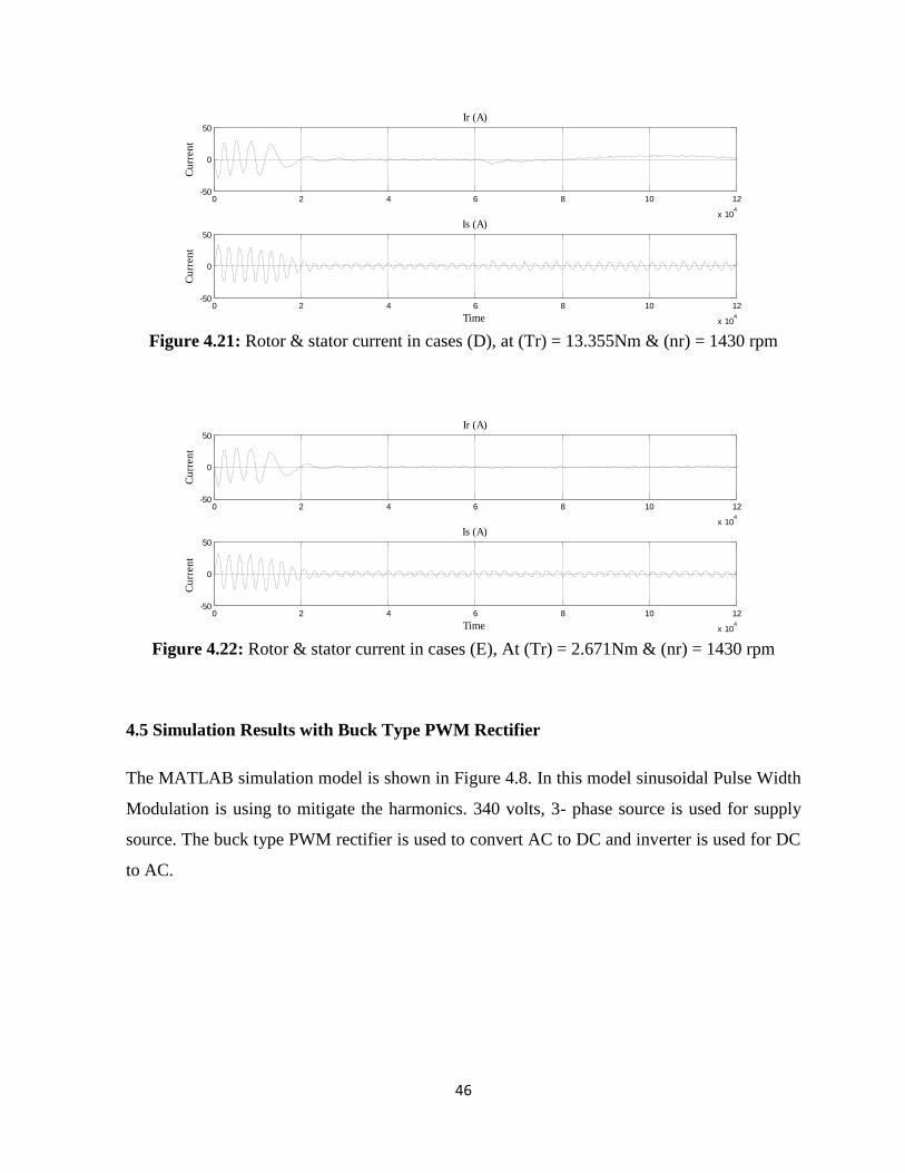
Figure 4.21: Ri & Si in cases (D), At (Tr) = 13.355Nm & (nr) = 1430 rpm…………… 46

Figure 4.22: Ri & Si in cases (E), At (Tr) = 2.671Nm & (nr) = 1430 rpm…………..… 46

Figure 4.23: Simulation Circuit of Buck type PWM rectifier harmonic technique…..… 47

Figure 4.24: Rotor speed in case (A), At (Tr) = 26.71Nm &(nr) =1430 rpm………...… 48

Figure 4.25: Rotor speed in case (B), At (Tr) = 26.71Nm &(nr) =715 rpm…….…….... 48

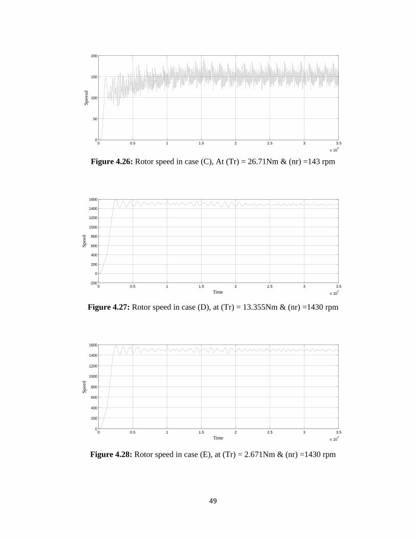
Figure 4.26: Rotor speed in case (C), At (Tr) = 26.71Nm & (nr) =143 rpm…....…..….. 49

Figure 4.27: Rotor speed in case (D), At (Tr) = 13.355Nm & (nr) =1430 rpm……….... 49

Figure 4.28: Rotor speed in case (E), At (Tr) = 2.671Nm & (nr) =1430 rpm………….. 49

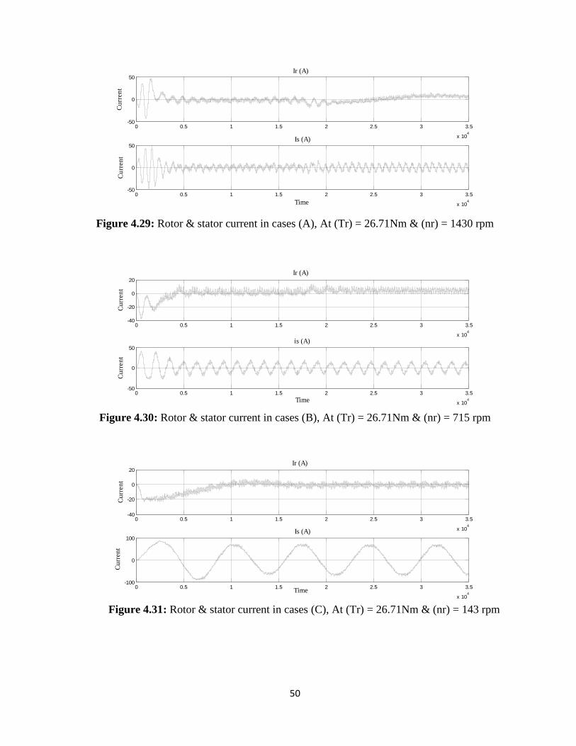
Figure 4.29: Ri & Si in cases (A), At (Tr) = 26.71Nm & (nr) = 1430 rpm……………... 50

Figure 4.30: Ri & Si in cases (B), At (Tr) = 26.71Nm & (nr) = 715 rpm………………. 50

Figure 4.31: Ri & Si in cases (C), At (Tr) = 26.71Nm & (nr) = 143 rpm………………. 50

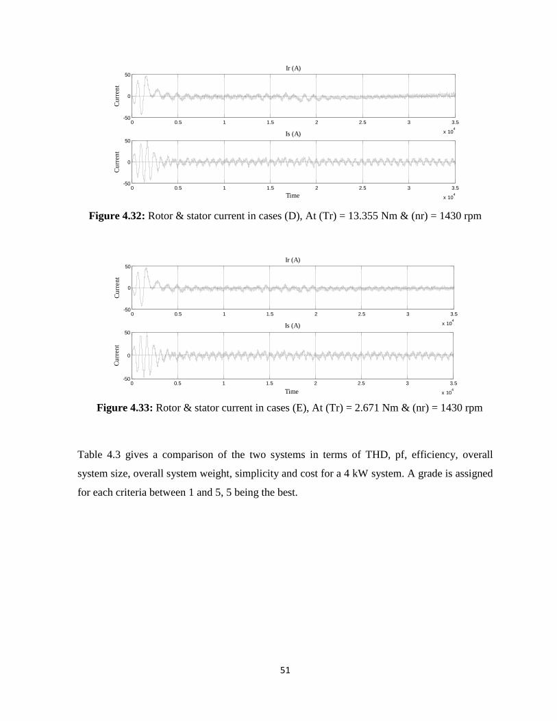
Figure 4.32: Ri & Si in cases (D), At (Tr) = 13.355Nm & (nr) = 1430 rpm………….… 51

Figure 4.33: Ri & Si in cases (E), At (Tr) = 2.671Nm & (nr) = 1430 rpm……………... 51

xii

Figure 4.34: Harmonics Chart Graph…………………………………………...……… 53

Figure A: Overall circuit diagram of simulation of 24-pulse Phase shift transformer…. 59

Figure B: Overall circuit diagram of simulation model of VFD with using PWM…….. 60

xiii

LIST OF SYMBOLS

i′ap: ia referred to Primary side

i′bp: ib referred to Primary side

i′cp: ic referred to Primary side

ABV : Line-to-Line Primary phasor

abV :

Line-to-Line Secondary phasor

ai :

Line current in secondary delta transformer

'ai : Line current in secondary delta transformer referred to primary

δ: Phase angle

Ȋn: Peak value of the nth

order harmonic current

N1: Primary winding number turns

'ani :

Phase angles of nth

order harmonic 'ani

ani : Phase angles of nth

order harmonicani

VAB: Primary Line voltage

N2: Secondary winding number turns

Vab: Secondary Line voltage

ia, ib, ic: Secondary Line current

xiv

LIST OF ABBREVIATIONS

AC : Alternative current

ASD : Adjustable speed drive

P : Active power

S : Apparent power

CSO : Current source output

CSI : Current source inverter

CFI : Current fed inverter

DC : Direct current

EMI : Electromagnetic Interference

fs Source frequency

GTO : Gate turn-off thyristor

I/P : Input voltage

IEEE : Institute of Electrical and Electronics Engineers

IEC : International Electro technical Commission

IGBT : Insulated gate bipolar transistor

Mi: Modulation index

PWM : Pulse width modulation

PCR : Phase controlled rectifier

PF : Power factor

Q : Reactive power

O/P : Output voltage

RMS : Root Mean Square

SMPS : Switch Mode Power Supply

THD : Total Harmonic Distortion

UPS : Uninterruptable power supply

VFD : Variable frequency drive

VSD : Variable speed drive

VSO : Voltage source output

xv

VSI : Voltage source inverter

VFI : Voltage fed inverter

1

CHAPTER 1

INTRODUCTION

This document has been created to give general information of power system harmonics, their

causes, effects and methods to control them especially when these harmonics are related to

variable frequency drives (or adjustable speed drives). Some of the subjects covered are

definition of harmonic, generation of harmonics, effects of harmonics and control of

harmonics. As the sin wave voltage is given to the load (linear), Furthermore, The load current

is directly proportional to the voltage, and impedance, as a result voltage waveform. Most

common linear-loads are resistive heaters, incandescent lamps and induction or synchronous

motors operating in the unsaturated region.

For some loads current and voltage are not proportional to each other. These loads are

classified as nonlinear loads. In this case current and voltage waveforms are non-sinusoidal

and contain distortions. The 50-Hz waveform has numerous additional waveforms

superimposed upon it creating multiple frequencies within the normal 50-Hz sine wave period.

The fundamental frequency multipliers are harmonics. Normally, harmonic current distortions

create harmonic voltage distortions. When the applied voltage source is stiff, meaning that no

matter how much current is drawn from it, its voltage will remain constant, and this will not be

a concern. Variable frequency motor drives (VFD), switch mode power supplies and battery

charges can be shown as the most prominent examples of nonlinear loads.

Power electronic devices are used in VFDs to adjust the amplitude and the frequency of the

voltage that is applied to the load. Pulse Width Modulation (PWM) is the most widespread

technique to obtain near sinusoidal currents for the motor windings. However, the dc bus

voltage needed by the inverter is typically obtained by a diode rectifier which draws non-

sinusoidal currents from the line, creating harmonic distortion in the line voltage. Harmonic

magnitudes should be limited to be able to have a clean and efficient power. Voltage and

current waveforms rich in harmonics may lead to following abnormal operations and

conditions in power systems (Svensson, 1999):

2

Due to voltage harmonics, it produces heating in induction, and synchronous motors

along with generators at all.

By the effect of voltage harmonics, the higher values can cause the reduction of

insulation levels results weaken insulation in winding as well as in capacitors.

Voltage distortions cause the malfunction of different electrical components.

Due to current harmonics, while winding of the motor, results EMI (Electro-magnetic

interference).

Current harmonics in motor windings can create electromagnetic interference (EMI).

Current distortion flowing through transformers& cables produce higher heating

additional with the heating that is produced by the fundamental signal.

Heat losses are increasing, as the current harmonics passes from circuit breakers, and

switch-gears.

In power system, different filtering topologies are used, create failure of capacitors or

in other equipment, all these issues are regarding to current harmonics produce

resonant currents.

Finally, harmonics results false tripping of circuit breakers, and relays failure which

used for protection of power systems.

1.1 Objective

Objective of the thesis is to investigate the effects of driving techniques of variable speed

motors on harmonic generation. In this context, simulations have been performed for an

induction motor driven by an inverter with two different front-end rectifiers. First a 24-pulse

rectifier obtained by phase shift transformers has been designed and tested by simulation.

Then a buck-type PWM rectifier has been designed and tested. Simulations have been carried

out for a 4 kW induction motor operating at different conditions. Results for each case has

been obtained and compared. It is concluded that both techniques can be effectively used to

keep the harmonics in related standards but the PWM rectifier is preferred since it is simpler,

cheaper and more compact.

3

1.2 Thesis Structure

In Chapter 1 general information of power system harmonics and objective of this thesis are

explained. In Chapter 2 harmonic issues in power systems are discussed. In Chapter 3 the

techniques used in this thesis are explained. Phase shift transformer structure is discussed and

its turns-ratios are calculated. Simulation results are given in Chapter 4. Chapter 5 gives the

conclusions.

4

CHAPTER 2

HARMONIC PROBLEMS IN POWER SYSTEMS

In this chapter, harmonic issues in power systems are discussed. Sources of harmonics are

explained and mitigation techniques are summarized. The two techniques that are used in this

thesis, multi-pulse rectifiers and PWM rectifiers are explained in more detail.

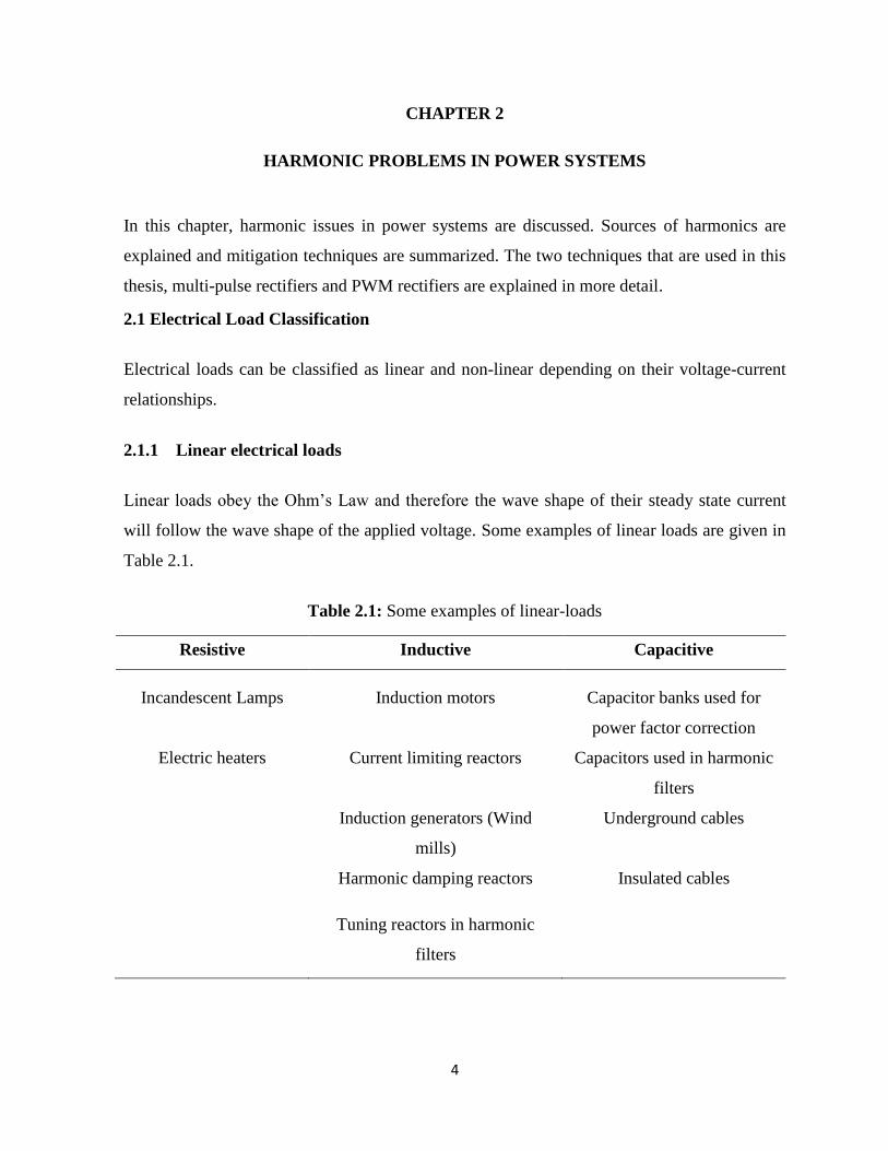
2.1 Electrical Load Classification

Electrical loads can be classified as linear and non-linear depending on their voltage-current

relationships.

2.1.1 Linear electrical loads

Linear loads obey the Ohm’s Law and therefore the wave shape of their steady state current

will follow the wave shape of the applied voltage. Some examples of linear loads are given in

Table 2.1.

Table 2.1: Some examples of linear-loads

Resistive Inductive Capacitive

Incandescent Lamps Induction motors Capacitor banks used for

power factor correction

Electric heaters Current limiting reactors Capacitors used in harmonic

filters

Induction generators (Wind

mills)

Underground cables

Harmonic damping reactors Insulated cables

Tuning reactors in harmonic

filters

5

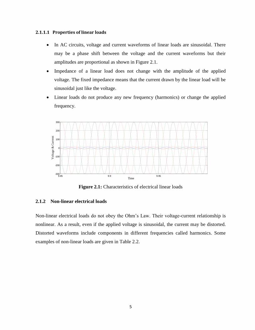
2.1.1.1 Properties of linear loads

In AC circuits, voltage and current waveforms of linear loads are sinusoidal. There

may be a phase shift between the voltage and the current waveforms but their

amplitudes are proportional as shown in Figure 2.1.

Impedance of a linear load does not change with the amplitude of the applied

voltage. The fixed impedance means that the current drawn by the linear load will be

sinusoidal just like the voltage.

Linear loads do not produce any new frequency (harmonics) or change the applied

frequency.

Figure 2.1: Characteristics of electrical linear loads

2.1.2 Non-linear electrical loads

Non-linear electrical loads do not obey the Ohm’s Law. Their voltage-current relationship is

nonlinear. As a result, even if the applied voltage is sinusoidal, the current may be distorted.

Distorted waveforms include components in different frequencies called harmonics. Some

examples of non-linear loads are given in Table 2.2.

9.85 9.9 9.95-300

-200

-100

0

100

200

300

Time

Vo

ltag

e &

Cu

rren

t

6

Table 2.2: Some examples of non- linear loads

Power electronics Arc devices

Variable frequency drives Fluorescent lighting

DC motor controllers Arc furnaces

Cycloconverters Welding machines

Cranes

Elevators

Steel mills

Power supplies

UPS

Battery chargers

2.1.2.1 Properties of non-linear loads

Non-linear loads change the shape of the current waveform from a sine wave to some

other form as shown in Figure 2.2.

Non-linear loads create harmonic currents in addition to the original (fundamental

frequency) AC current. Under these conditions, the voltage waveform is no longer

proportional to the current.

Impedance of non-linear loads changes with the amplitude of the applied voltage. The

changing impedance means that the current drawn by the non-linear load will not be

sinusoidal even when it is connected to a sinusoidal voltage. These non-sinusoidal

currents contain harmonic currents that interact with the impedance of the power

distribution system to create voltage distortion that can affect both the distribution

system equipment and the loads connected to it.

7

Figure 2.2: Characteristics of non-linear load

2.2 Power Factor in Electrical Power Systems

Power factor is an important parameter for the loads of distribution systems. Industrial

consumers are required to use power factor correction (PFC) systems to keep the power factor

in certain limits to reduce the amount of reactive power drawn from the line. Traditional PFC

methods typically focus on displacement power factor and therefore do not achieve the total

energy savings available in facilities having both linear and non–linear loads. Only a through

Total Power Factor Correction can the savings and power quality be maximized (Sandoval,

2014).

2.2.1 Power factor with linear loads

When the loads connected to the system are linear and the voltage is sinusoidal, the power

factor is calculated with the following equation:

Pf = COS( ) (2.1)

It can also be defined as the ratio of active power to apparent.

P

SPf =

(2.2)

When the loads are linear and the voltage is sinusoidal, the active, reactive and apparent

powers are calculated mathematically with the following equations:

0.9 0.91 0.92 0.93 0.94 0.95 0.96 0.97 0.98 0.99 1-300

-200

-100

0

100

200

300

Time

Vo

ltag

e &

Cu

rren

t

8

P = VI cos( )

(2.3)

Q = VI sin( ) (2.4)

S = VI (2.5)

Figure 2.3 shows these relationships in phasor forms.

If the power factor is low, a smaller portion of the total power is used to create work, which is

called active power (P), and the rest is known as reactive power (Q). Power factor can be

improved by power factor correction systems to minimize the reactive power and maximize

the active power. The most common technique used in power factor correction is connecting a

Figure 2.3: Power triangle

Figure 2.4: Power triangle with capacitor bank

9

capacitor bank in parallel with the load (Sandoval, 2014). This is called compensation. Effect

of compensation is shown in Figure 2.4. When a capacitor is added the phase angle is reduced

and thus cos𝜑2 > cos𝜑1.

2.2.2 Power factor for non–linear loads under sinusoidal voltage

When the loads are non–linear but the applied voltage is sinusoidal, the current has harmonics

and the active, reactive and apparent power should not be calculated using traditional methods.

In this case, only the fundamental harmonic of the load current contributes to the active power

generation. Therefore active power is defined as

1 1cos( )P = VI (2.6)

Where I1 is the fundamental current and 𝜑1 is the phase angle between the voltage and

fundamental current.

Total Harmonic Distortion (THD) is an important power quality parameter and shows how

distorted a waveform is. THD of the current signal is defined as

2

2

1

I

I(THD)

n

n

i

(2.7)

Where In is the rms value of the nth

harmonic since

2

I = I2

nn

(2.8)

THD can be rewritten as

2 2 21

1 1

I I I1

I I(THD)

n n

i

(2.9)

Therefore, the RMS value of current can also be expressed as a function of THD, as well as

fundamental current value is mentioned in Equation.(2.10).

10

2I = I 1 + THD1 1 (2.10)

By using the equations (2.5), (2.6) and (2.10), total power factor can be calculated in

Equation.(2.11)

1

pf = cos(φ )1 21 + THD1

(2.11)

There are two terms involved in the calculation of the power factor: (cos𝜑1) and

21 1 + THD1

. The term (cos𝜑1) is called the displacement power factor pfdisp since it is

the cosine of the phase angle between the voltage and the fundamental component of the

current, similar to the power factor calculated with linear loads under sinusoidal voltage. The

term 21 1 + THD1

is called distortion power factor pfdist . Total Power Factor pfT

obtained mathematically as in Equation. (2.12):

pfT = pfdisp × pfdist (2.12)

Total power factor decreases if and only if the angle between the voltage and fundamental

current grows due to increase in the reactive power. Similarly if the (THD)i increases the total

power factor decreases. Because of distortion, total power factor is always lower than the

displacement power factor.

Total power factor correction can only be achieved when both displacement power factor and

distortion power factor are corrected. Therefore, the displacement angle between voltage and

current should be reduced and the total harmonic current distortion should be minimized. If

both of these measures are not taken together, the total power factor may still be improved but

it may not be enough to meet the demands of the utility.

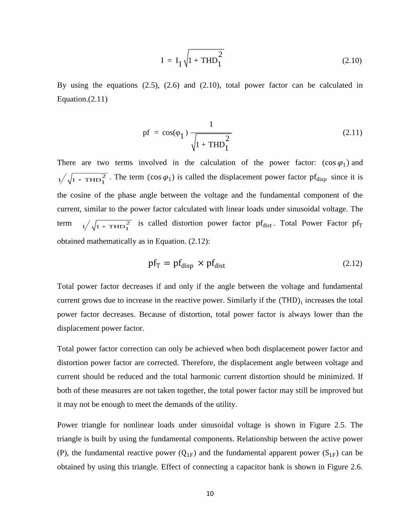
Power triangle for nonlinear loads under sinusoidal voltage is shown in Figure 2.5. The

triangle is built by using the fundamental components. Relationship between the active power

(P), the fundamental reactive power (Q1F) and the fundamental apparent power (S1F) can be

obtained by using this triangle. Effect of connecting a capacitor bank is shown in Figure 2.6.

11

Reactive power supplied by the capacitor (QCF ) reduces the reactive power supplied by the

line. However, there is always the risk of resonance between the capacitor bank and the

inductive transformer winding.

2.2.3 Power factor for non-linear loads under distorted supply voltage

When the loads are non–linear and the voltage is distorted, the active, reactive and apparent

power cannot be calculated by using the previous equations. Now, each harmonic component

Figure 2.5: Power triangle in non-linear load and sinusoidal voltage

no

Figure 2.6: Power triangle in non-linear load and sinusoidal voltage with capacitor bank

12

of the voltage and current can contribute to the total active power. Therefore, voltage and

current components at each harmonic frequency should be included in the summing equation.

As the phase angles of the voltage harmonics can be neglected, total active power equation can

be expressed as follows:

NP = V I cos(φ )n n n

n=1 (2.13)

Mathematically Power factor calculated by

NV I cos(φ )n n n

n=1pf =

VI

(2.14)

However, the voltage rms value is a function of the total harmonic voltage distortion and the

rms value of the fundamental component of voltage:

2V = V 1 + THD1 V

(2.15)

By applying equations (2.10),(2.14) and (2.15), the power factor can be obtained as:

P 1pf = *

2 2S 1 + THD * 1 + THD1 I V

(2.16)

2 21 1 + THD * 1 + THDI V

is the distortion power factor. Its value depends on both the

voltage distortion and the current distortion. So,

Ppf = pfT dist

S1

(2.17)

The term P S1 can be written as:

13

N

V I cos φn n nV I cos φP 1 1 1 n=2= +

S S S1 1 1

(2.18)

Where V I cos( ) S1 1 1

is the displacement power factor. So,

N

V I cos φn n nn=2

pf = pf + pfT disp distS1

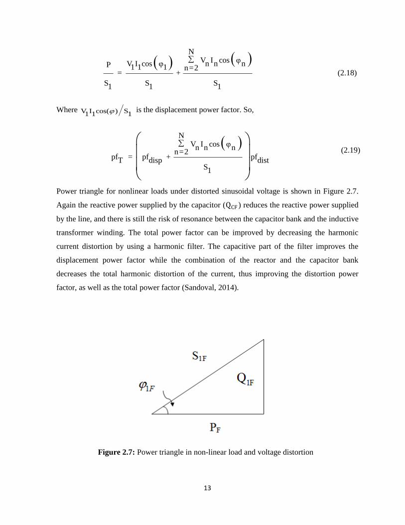
Power triangle for nonlinear loads under distorted sinusoidal voltage is shown in Figure 2.7.

Again the reactive power supplied by the capacitor (QCF ) reduces the reactive power supplied

by the line, and there is still the risk of resonance between the capacitor bank and the inductive

transformer winding. The total power factor can be improved by decreasing the harmonic

current distortion by using a harmonic filter. The capacitive part of the filter improves the

displacement power factor while the combination of the reactor and the capacitor bank

decreases the total harmonic distortion of the current, thus improving the distortion power

factor, as well as the total power factor (Sandoval, 2014).

(2.19)

Figure 2.7: Power triangle in non-linear load and voltage distortion

no

14

2.3 Variable Frequency Drives

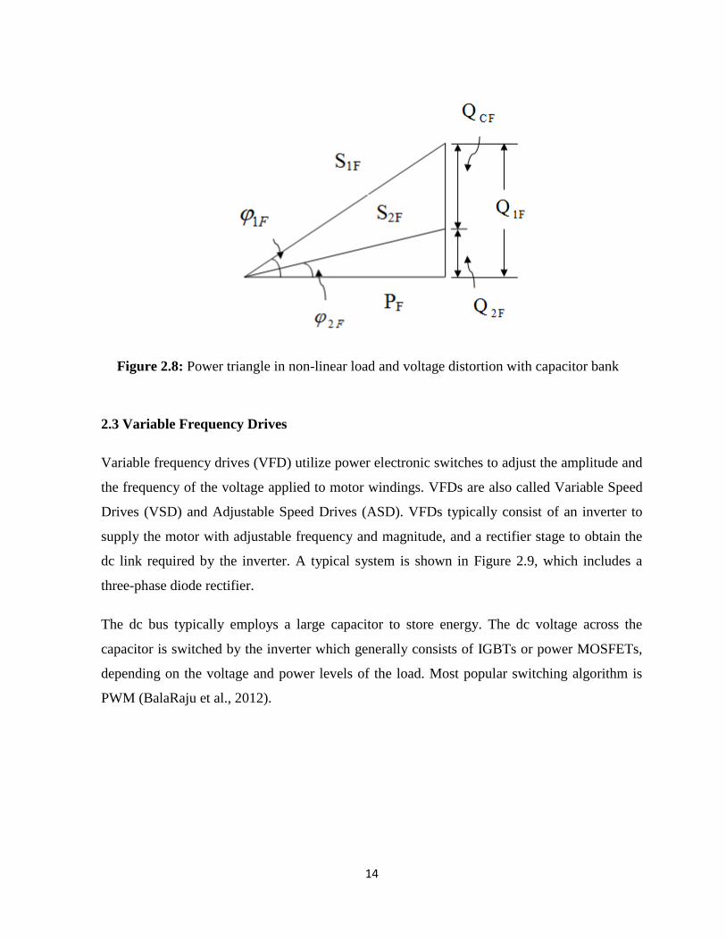
Variable frequency drives (VFD) utilize power electronic switches to adjust the amplitude and

the frequency of the voltage applied to motor windings. VFDs are also called Variable Speed

Drives (VSD) and Adjustable Speed Drives (ASD). VFDs typically consist of an inverter to

supply the motor with adjustable frequency and magnitude, and a rectifier stage to obtain the

dc link required by the inverter. A typical system is shown in Figure 2.9, which includes a

three-phase diode rectifier.

The dc bus typically employs a large capacitor to store energy. The dc voltage across the

capacitor is switched by the inverter which generally consists of IGBTs or power MOSFETs,

depending on the voltage and power levels of the load. Most popular switching algorithm is

PWM (BalaRaju et al., 2012).

Figure 2.8: Power triangle in non-linear load and voltage distortion with capacitor bank

15

Figure 2.9: VFD system (BalaRaju et al., 2012)

2.4 Harmonics Mitigation

There are many techniques to mitigate the effects of harmonics. Before applying those

techniques, one should know which harmonic frequencies are more effective and which ones

are not. Typically the lowest harmonic is the third one since mostly three-phase loads are used.

The exception is highly nonlinear loads such as arc furnaces. Arc furnaces create second order

harmonics too. The impact and elimination of these harmonics are out of the scope of this

thesis.

In three-phase system harmonics of the 3rd

order and its multiples (3rd

, 6th

, 9th

etc.) cancel each

other because there are 120° phase shifts between the voltages. Remaining harmonics are the

5th

, 7th

, 11th

, 13th

… harmonics. Naturally, amplitudes of the first few harmonics are greater,

and the magnitude rolls down as the harmonic order increases. Typically, 5th

, 7th

, and 11th

harmonics are the most important ones (BalaRaju et al., 2012).

Nonlinear loads and distorted currents produce distorted voltage drops across the line

impedances. As a result, non-sinusoidal voltages appear across the other loads which are

connected to the same line. Extra losses in the lines and windings of the transformers and

16

generators, and extra iron losses in the transformer and generator cores are generated as a

result of these non-sinusoidal currents and voltages. Therefore, it is required to reduce the

harmonics under certain levels set forth by standards such as IEEE 519-1992 in the USA and

IEC 61000-3-2/IEC 61000-3-4 in Europe (Manlinowski, 2001).

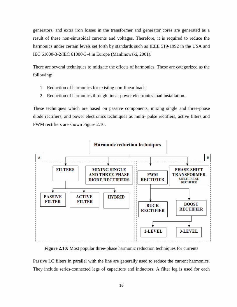
There are several techniques to mitigate the effects of harmonics. These are categorized as the

following:

1- Reduction of harmonics for existing non-linear loads.

2- Reduction of harmonics through linear power electronics load installation.

These techniques which are based on passive components, mixing single and three-phase

diode rectifiers, and power electronics techniques as multi- pulse rectifiers, active filters and

PWM rectifiers are shown Figure 2.10.

Figure 2.10: Most popular three-phase harmonic reduction techniques for currents

Passive LC filters in parallel with the line are generally used to reduce the current harmonics.

They include series-connected legs of capacitors and inductors. A filter leg is used for each

17

harmonic to be filtered. Typically, a leg is used for the fifth, another one for the seventh and

another one to reduce the 11th

and 13th

harmonics together. Passive filters are cheap and

simple (Manlinowski, 2001). However, they also have some disadvantages such as below:

1- Separate filters should be designed for each installation and application.

2- High fundamental current result in extra power losses.

3- Filters are heavy and bulky.

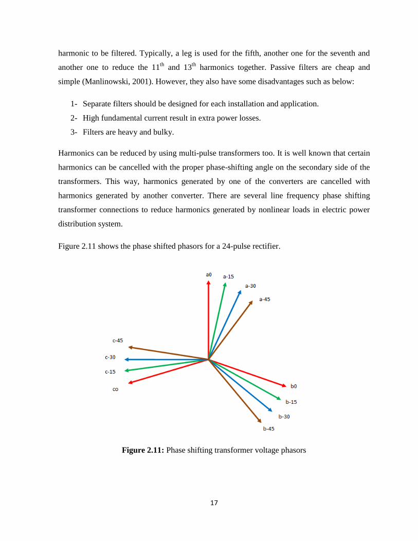
Harmonics can be reduced by using multi-pulse transformers too. It is well known that certain

harmonics can be cancelled with the proper phase-shifting angle on the secondary side of the

transformers. This way, harmonics generated by one of the converters are cancelled with

harmonics generated by another converter. There are several line frequency phase shifting

transformer connections to reduce harmonics generated by nonlinear loads in electric power

distribution system.

Figure 2.11 shows the phase shifted phasors for a 24-pulse rectifier.

Figure 2.11: Phase shifting transformer voltage phasors

18

The phase shifting transformer reduction method, possesses several drawbacks like bulky and

heavy transformer, excessive voltage drop, and increased harmonic currents at non-

symmetrical load.

PWM rectifiers are also used for harmonic mitigation. These rectifiers replace the

uncontrolled diode rectifier. The input current for these rectifiers can be made near sinusoidal

with zero phase shift. They can provide constant output voltage or current. They can also

boost the input voltage (boost type PWM rectifier) or reduce it (buck type PWM rectifier)

(Manlinowski, 2001).

Main properties of PWM-rectifiers are as follows:

1- Power can flow in both directions.

2- Input current is nearly sinusoidal.

3- Unity input power factor is possible.

4- Input current total harmonic distortion is very low (under 5%).

5- Adjustment and stabilization of DC-link voltage or current is possible.

6- Capacitor or inductor size is lowered due to the continuous current.

2.4.1 Phase displacement of harmonic currents

The phases of the harmonic currents are shifted when they are reflected from the secondary to

the primary of a phase-shifting transformer. This makes it possible to cancel certain harmonic

currents generated by a non-linear load (Wu, 2006). A ∆-Y connected transformer supplying a

non-linear load is shown in Figure 2.12.

Assuming that the ratio of the line-to-line voltages is unity, the turn ratio is found as

N / N = 31 2

The phase difference between the "line-to-line" voltage of the primary and secondary of the

transformer is

δ = V - V = -30°ab AB

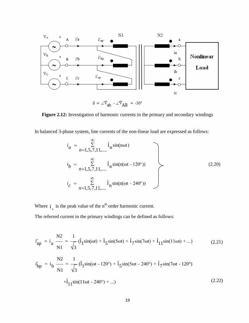
19

Figure 2.12: Investigation of harmonic currents in the primary and secondary windings

In balanced 3-phase system, line currents of the non-linear load are expressed as follows:

I sin(nωt)n1,5,7,11,....

ian

I sin(n(ωt - 120 ))n1,5,7,11,....

ibn

(2.20)

I sin(n(ωt - 240 ))n1,5,7,11,....

icn

Where In

is the peak value of the nth

order harmonic current.

The referred current in the primary windings can be defined as follows:

N2 1ˆ ˆ ˆ ˆ= i = (I sin(ωt) + I sin(5ωt) + I sin(7ωt) + I sin(11ωt) + ...)ap a 1 5 7 11

N1 3

i

N2 1ˆ ˆ ˆ= i = (I sin(ωt - 120°) + I sin(5ωt - 240°) + I sin(7ωt - 120°)bp b 1 5 7

N1 3

i

11ˆ+I sin(11ωt - 240°) + ...)

(2.21)

(2.22)

20

Line current in the primary can be now calculated:

ˆ ˆ= I sin(ωt + 30°) + I sin(5ωt - 30°)ap bp 1 5i i ia ˆ+I sin(7ωt + 30°)7

ˆ+I sin(11ωt - 30°) + ...11

ˆ ˆI sin(nωt ) I sin(nωt + δ)n n1,7,13,... 5,11,17,...

δn n

In the right side of this equation the first term sums all the positive sequence harmonic

currents (n = 1, 7, 13, etc.) while the second term sums the negative sequence harmonics (n =

5, 11, 17, etc.).

When the harmonic components of the reflected line currents in Equation (2.23) are compared

to those of the secondary expressed in Equations (2.20), it is seen that the phase is shifted

backward for the positive sequence harmonics, and forward for the negative sequence ones:

i i δan an

for n=1, 7, 13, 19,… Positive sequence

i i δan an for n=5, 11, 17, 23,… Negative sequence

Hereani and

ani are the phase angles of harmonic currents for the primary and

secondary. This equation is valid for any phase angle (Wu, 2006).

2.4.2 Harmonic Cancellation

Harmonic current cancellation using a phase shifting transformer connection is shown in this

section for a 12-pulse system, shown in Figure 2.13. The phase shifting angle δ is 0° for the Y

connected secondary, and 30° for the Δ connected secondary windings (Wu, 2006).

Let’s the ratio of the line-to-line voltages be VAB Vab = VAB Va b = 2.The line currents in the

secondary windings then can be expressed as follows:

I sin(nωt)...n1,5,7,11,13,...

ian

(2.24)

(2.25)

(2.23)

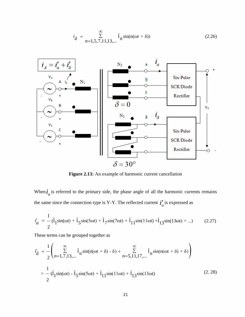
21

I sin(n(ωt + δ))n1,5,7,11,13,...

ian

(2.26)

Figure 2.13: An example of harmonic current cancellation

Whenai is referred to the primary side, the phase angle of all the harmonic currents remains

the same since the connection type is Y-Y. The reflected current ai is expressed as

1ˆ ˆ ˆ ˆ= (I sin(ωt) + I sin(5ωt) + I sin(7ωt) + I sin(11ωt)1 5 7 11

2

ia ˆ+I sin(13ωt) + ...)13 (2.27)

These terms can be grouped together as

1ˆ ˆI sin(n(ωt + δ) - δ) I sin(n(ωt + δ) + δ)n n

1,7,13,... 5,11,17,...2

ian n

1ˆ ˆ ˆ ˆ= (I sin(ωt) - I sin(5ωt) + I sin(11ωt) + I sin(13ωt)1 5 11 13

2

(2. 28)

22

For δ = 30° the total primary line current Ai is

ˆ ˆ ˆi = i + i = I sinωt + I sin11ωt + I sin13ωtA a a 1 11 13

ˆ+I sin23ωt + ...23 (2.29)

In this equation the 5th

, 7th

, 17th

, and 19th

harmonic currents in ai and

ai are 180° out of

phase. Therefore these harmonics cancel each other (Wu, 2006).

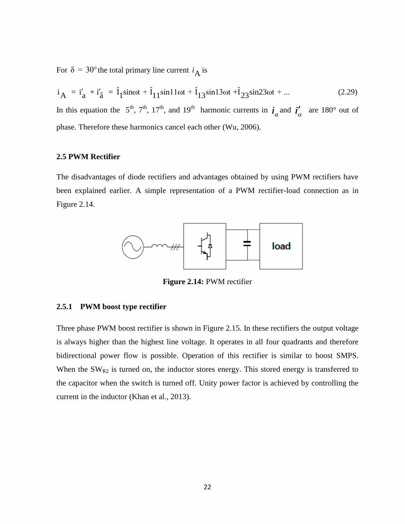
2.5 PWM Rectifier

The disadvantages of diode rectifiers and advantages obtained by using PWM rectifiers have

been explained earlier. A simple representation of a PWM rectifier-load connection as in

Figure 2.14.

Figure 2.14: PWM rectifier

2.5.1 PWM boost type rectifier

Three phase PWM boost rectifier is shown in Figure 2.15. In these rectifiers the output voltage

is always higher than the highest line voltage. It operates in all four quadrants and therefore

bidirectional power flow is possible. Operation of this rectifier is similar to boost SMPS.

When the SWR2 is turned on, the inductor stores energy. This stored energy is transferred to

the capacitor when the switch is turned off. Unity power factor is achieved by controlling the

current in the inductor (Khan et al., 2013).

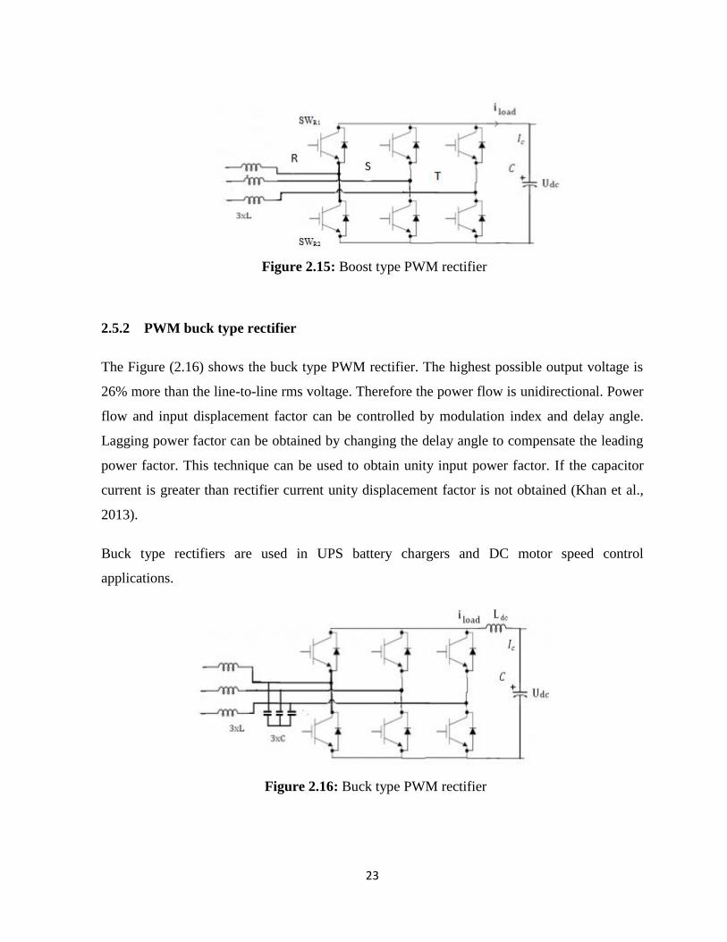
23

Figure 2.15: Boost type PWM rectifier

2.5.2 PWM buck type rectifier

The Figure (2.16) shows the buck type PWM rectifier. The highest possible output voltage is

26% more than the line-to-line rms voltage. Therefore the power flow is unidirectional. Power

flow and input displacement factor can be controlled by modulation index and delay angle.

Lagging power factor can be obtained by changing the delay angle to compensate the leading

power factor. This technique can be used to obtain unity input power factor. If the capacitor

current is greater than rectifier current unity displacement factor is not obtained (Khan et al.,

2013).

Buck type rectifiers are used in UPS battery chargers and DC motor speed control

applications.

Figure 2.16: Buck type PWM rectifier

24

CHAPTER 3

PHASE SHIFT TRANSFORMER AND BUCK TYPE PWM RECTIFIER

Variable Frequency Drives (VFD) utilizes a frond end rectifier to obtain the required DC bus

voltage for the inverter. This rectifier could be a diode rectifier (uncontrolled) or PWM

rectifier (controlled). Diode rectifiers have the worst harmonic distortion due to the large

capacitor connected at its output. PWM rectifiers use high frequency switching to synthesize

near sinusoidal input currents. Another technique that can be used at high power levels is to

include a phase-shifting transformer at the input to have multi-pulse rectified voltage causing a

better harmonic content.

In this chapter, these three structures are explained in more detail.

3.1 Phase Shift Transformer

A 24-pulse rectifier topology based on phase shifting by conventional magnetic, is used at

high power levels. Four 3-phase systems can be obtained from a single 3-phase source using

single-phase and 3-phase transformers (Wu, 2006). As shown in Figure 3.1.Two seriously

connected six-pulse rectifiers in the upper side are fed from the 30º displaced secondary

windings of a three phase transformer, yielding 12-pulse rectified output. One of the two

seriously connected diode rectifiers at the bottom is fed from the secondary windings of Y-Δ

connected single-phase transformer while the other one is fed from the secondary windings of

another three phase transformer. The phase-shift of the voltages applied to all rectifiers are 15º

yielding a 24-pulse rectified output voltage (Arvindan, 2010).

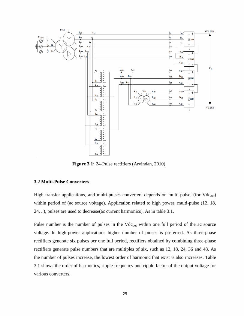
25

Figure 3.1: 24-Pulse rectifiers (Arvindan, 2010)

3.2 Multi-Pulse Converters

High transfer applications, and multi-pulses converters depends on multi-pulse, (for Vdcout)

within period of (ac source voltage). Application related to high power, multi-pulse (12, 18,

24, ..), pulses are used to decrease(ac current harmonics). As in table 3.1.

Pulse number is the number of pulses in the Vdcout within one full period of the ac source

voltage. In high-power applications higher number of pulses is preferred. As three-phase

rectifiers generate six pulses per one full period, rectifiers obtained by combining three-phase

rectifiers generate pulse numbers that are multiples of six, such as 12, 18, 24, 36 and 48. As

the number of pulses increase, the lowest order of harmonic that exist is also increases. Table

3.1 shows the order of harmonics, ripple frequency and ripple factor of the output voltage for

various converters.

26

Table 3.1: Harmonics and ripple variation with pulse number (Arvindan, 2010)

No. of Pulses Harmonic numbers Frequency Ripple factor

(%)

1 1,2,3,… 1*fs 121

2 1,3,5,… 2*fs 48.2

3 2,4,5,… 3*fs 18.2

6 5,7,11,… 6*fs 4.2

12 11,13,23,… 12*fs 1

18 17,19,35,… 18*fs 0.64

24 23,25,47,… 24*fs 0.22

3.2.1 Bidirectional multi-pulse rectifier

These thyristorized converters provide harmonic reduction through pulse multiplication with

the aid of magnetics. Bidirectional power flow and adjustable output dc voltage are obtained

by utilizing fully controlled thyristor bridge converters. A multiple winding transformer is

used at the input to allow multi pulse rectification. Pulse multiplication is made possible by

using tapped reactors. Input current THD and output voltage ripple are low. These converters

are especially useful for dc motor drives operating at high powers and HVDC transmission

systems. Autotransformers can help reduce the "cost" and "weight" of input transformers in

low- and medium-voltage applications (Arvindan, 2010).

3.2.2 Unidirectional multi-pulse converters

By using similar magnetic structures to Bidirectional Multi-pulse Rectifiers, unidirectional

converters can be obtained for high pulse numbers all the way from 12 to 48.

Autotransformers can be used for this purpose with phase splitting (Arvindan, 2010).

27

3.3 Design of 24-Pulse Rectifier

Figure 3.1 represents the investigated 24-pulse rectifier topology. The whole system is

supplied by one three-phase transformers with Y-Δ secondary. Phase shifted outputs of this

secondary is used at the input of two other three-phase transformers, constructed by using six

single-phase transformer. There is another three-phase with Y-Δ secondary supplied by the

output of these single-phase transformers. Overall there are four individual 3-phase systems.

The phase shift for a topology with a certain number rectifiers is given as follows:

Phase shift = 60°/No. of bridge

Harmonics that are created by these transformers are at the following frequencies:

Harmonics = nk ± 1

Where n is the number of bridges used in the system and k = 1, 2, 3,…

So, as the numbers of bridges go up, so does the minimum order of harmonic (Arvindan,

2010).

3.3.1 One to four, 3-phase system

In Figure 3.1, the source lines A0,B0,C0 feeds the Yy0d1, 3-ph., 3-winding, step down

transformer and two 3-ph. systems, one (represented as a0, b0 and c0) with line voltages (Va0,b0,

Vb0,c0, Vc0,a0) in phase with the source line voltages and the other (represented as a-30, b-30

and c-30) with line voltages (Va-30,b-30, Vb-30,c-30, Vc-30,a-30) lagging the source line voltages by

30º are obtained from the secondary Y (y0) and Δ (d1) windings respectively. The line

voltages Va0,b0, Vb0,c0, Vc0,a0 and Va-30,b-30, Vb-30,c-30, Vc-30,a-30 are shown in Figures 3.2 and 3.3

respectively. It should be noted that only the phase angles of the six line voltages of the 3-

phase systems are different. Voltages of these lines have the same magnitude. The six line

voltages Va0,b0, Vb0,c0, Vc0,a0, Va-30,b-30, Vb-30,c-30, Vc-30,a-30 are isolated using 6 single-phase

transformers with appropriate turns ratio. The secondary voltages of the 1- phase transformers

corresponding to Va0,b0 and Va-30,b-30 are connected in series in order to yield Va-15,b-15, a

28

voltage equal in magnitude to the six line voltages but lagging Va0,b0 by 15º. This 15º phase

shift is by phasor sum of appropriate line voltages (Arvindan, 2010).

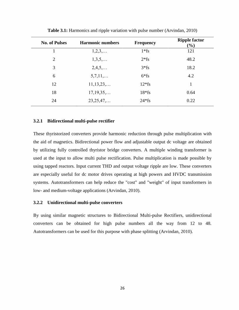
Figure 3.2: Input line Va0,b0, Vb0,c0 and Vc0,a0 at DBI

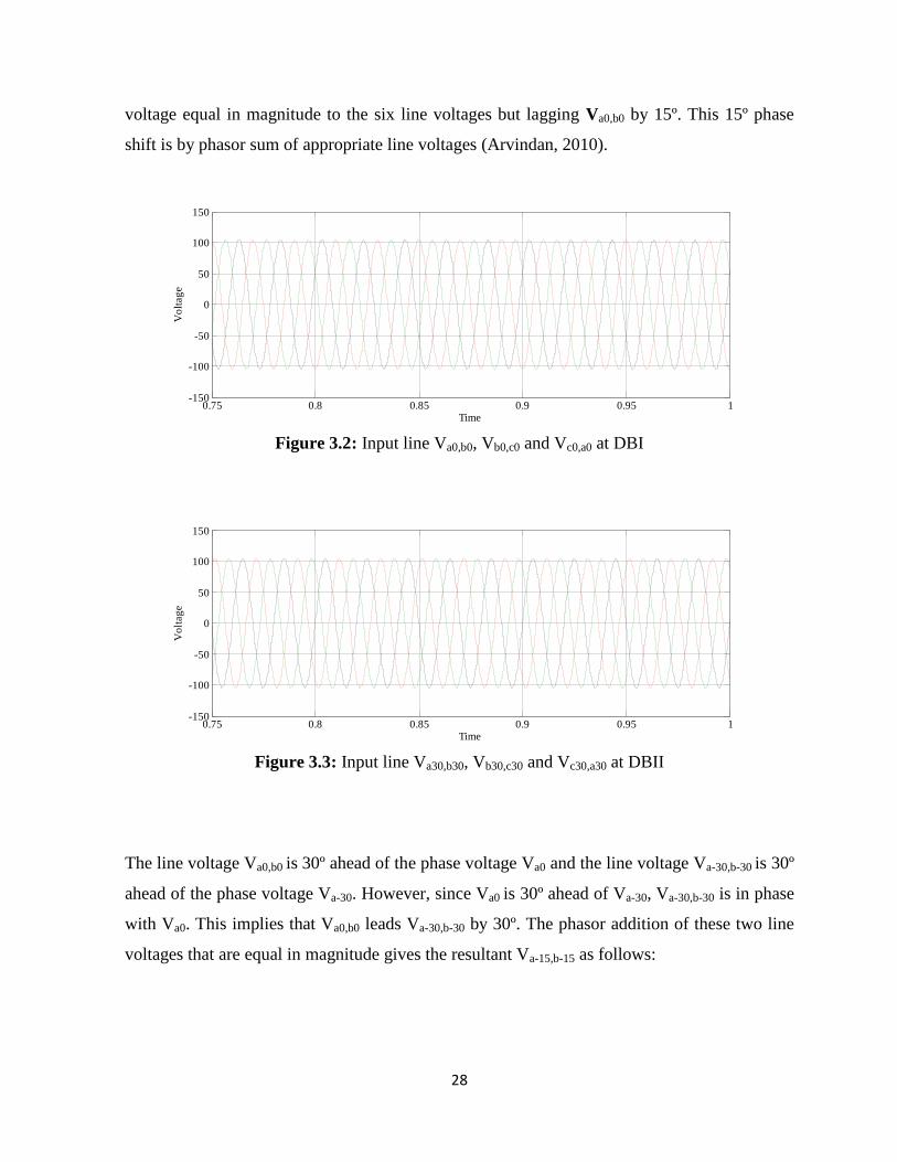
Figure 3.3: Input line Va30,b30, Vb30,c30 and Vc30,a30 at DBII

The line voltage Va0,b0 is 30º ahead of the phase voltage Va0 and the line voltage Va-30,b-30 is 30º

ahead of the phase voltage Va-30. However, since Va0 is 30º ahead of Va-30, Va-30,b-30 is in phase

with Va0. This implies that Va0,b0 leads Va-30,b-30 by 30º. The phasor addition of these two line

voltages that are equal in magnitude gives the resultant Va-15,b-15 as follows:

0.75 0.8 0.85 0.9 0.95 1-150

-100

-50

0

50

100

150

Time

Vo

ltag

e

0.75 0.8 0.85 0.9 0.95 1-150

-100

-50

0

50

100

150

Time

Vo

ltag

e

29

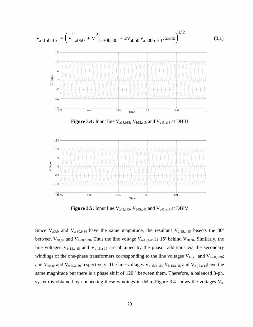
1/2

2 2V = V + V + 2V V Cos30a-15b-15 a0b0 a-30b-30 a0b0 a-30b-30

(3.1)

Figure 3.4: Input line Va15,b15, Vb15,c15 and Vc15,a15 at DBIII

Figure 3.5: Input line Va45,b45, Vb45,c45 and Vc45,a45 at DBIV

Since Va0b0 and Va-30,b-30 have the same magnitude, the resultant Va-15,b-15 bisects the 30º

between Va0,b0 and Va-30,b-30. Thus the line voltage Va-15,b-15 is 15º behind Va0,b0. Similarly, the

line voltages Vb-15,c-15 and Vc-15,a-15 are obtained by the phasor additions via the secondary

windings of the one-phase transformers corresponding to the line voltages Vb0,c0 and Vb-30,c-30;

and Vc0,a0 and Vc-30,a-30 respectively. The line voltages Va-15,b-15, Vb-15,c-15 and Vc-15,a-15have the

same magnitude but there is a phase shift of 120 º between them. Therefore, a balanced 3-ph.

system is obtained by connecting these windings in delta. Figure 3.4 shows the voltages Va-

0.75 0.8 0.85 0.9 0.95 1-150

-100

-50

0

50

100

150

Time

Vo

ltag

e

0.75 0.8 0.85 0.9 0.95 1-150

-100

-50

0

50

100

150

Time

Vo

ltag

e

30

15,b-15, Vb-15,c-15 and Vc-15,a-15. Hence, in Figure 3.1 the (phasors) lines a-15, b-15 and c-15 are

obtained and are fed to a 3-phase. transformer of the Yd1 configuration which provides a

phase shift of -30º i.e. 30º laggingº and hence, yields the (phasors) lines a45, b45 and c45

respectively. The corresponding line voltages Va-45,b-45, Vb-45,c-45 and Vc-45,a-45 that lag by 30º

the voltages Va-15,b-15, Vb-15,c-15 and Vc-15,a-15 respectively are shown in Figure 3.5. Thus, four 3-

ph. systems with successive 3-phase. systems displaced by 15º are realized (Arvindan, 2010).

3.3.2 Implementation of rectifier topology

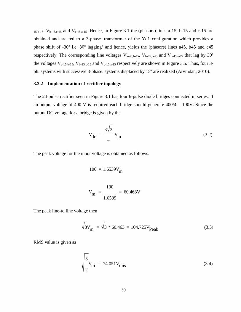
The 24-pulse rectifier seen in Figure 3.1 has four 6-pulse diode bridges connected in series. If

an output voltage of 400 V is required each bridge should generate 400/4 = 100V. Since the

output DC voltage for a bridge is given by the

3 3V = Vdc m

π

(3.2)

The peak voltage for the input voltage is obtained as follows.

100 = 1.6539Vm

100V = = 60.463Vm

1.6539

The peak line-to line voltage then

3V = 3 * 60.463 = 104.725Vm Peak

(3.3)

RMS value is given as

3V = 74.051Vm rms

2

(3.4)

31

3.3.3 Transformers turns ratio

The main transformer in the system is a 3-phase, 3-winding transformer with Yyod1 vector

configuration. The primary Y winding is connected to the 3- phase 268.7V utility.

Main transformer Yyod1: The two upper diode bridges are supplied from the y0 and d1

secondary windings. The winding turn’s ratio for the Yyo mathematically obtained as follows:

Y-primary Vline (rms)=268.7V

Vo secondary desired line voltage = 74.05V

N2/N1 = 74.05/268.7= 0.275

Similarly the winding turns ratio for the Yd1 mathematically obtained as follows:

Y-primary Vline (rms)= 268.7V

d1 secondary desired line voltage = 74.05V

N2/N1 =(74.05* 3 )/268.7= 0.477

Single-phase transformers

Primary windings of the six single-phase transformers are used to isolate the Y (y0) and Δ (d1)

secondary windings of the main transformer. The six secondary windings of the single-phase

transformers are divided into three pairs, with each pair containing two relevant secondary

windings corresponding to the voltage combinations Va0,b0 and Va-30,b-30, Vb0,c0 and Vb-30,c-30

and Vc0,a0 and Vc-30,a-30 that are synthesized by series cascade connection to obtain the line

voltages Va-15,b-15, Vb-15,c-15 and Vc-15,a-15 respectively. The synthesis of the voltage

combinations is as per Equation (3.1) yields Va-15,b-15 as follows:

Va0,b0 = 74.05 30° V

Va-30,b-30 = 74.05 0° V

Va-15,b-15 = 2 2

74.05 + 74.05 + 2 * 74.05 * 74.05 * cos30° V

Va-15,b-15 = 143.05 15° V

32

Similarly, the line voltages Vb-15,c-15 and Vc-15,a-15 are obtained by the synthesis of the relevant

voltage combinations. The synthesis yields magnitudes as follows:

V = V = V = 143.05a-15b-15 b-15c-15 c-15a-15 V

The three secondary pairs are connected in Δ to form a 3- phase winding. The Δ winding feeds

the third diode bridge and the desired magnitudes of the line voltages have to be as follows:

V = V = V = 74.05Va-15b-15 b-15c-15 c-15a-15

Turns ratio of each single-phase transformers is

N2/N1 = 74.05/143.05 = 0.5176 0.52

3-phase Y/d1 transformer

The voltages Va-15,b-15, Vb-15,c-15, and Vc-15,a-15 are fed to a Yd1 transformer to obtain line

voltages Va-45,b-45, Vb-45,c-45 and Vc-45,a-45 that are 300 behind the input Y voltages and supply

the fourth diode bridge. The magnitudes of the line voltages on Y and delta sides must be

equal.

V = V = V = V = V = V = 74.05a-15b-15 b-15c-15 c-15a-15 a-45b-45 b-45c-45 c-45a-45 V

Thus, the turns is given by

N2/N1 = 3 =1.732

3.4 Inverter

The dc bus voltage is switched at high frequency to obtain the adjustable frequency, adjustable

magnitude voltage necessary for the motor. Figure 3.6 shows the structure for the phase-

shifting transformer case (Bhattacharya, 2014).

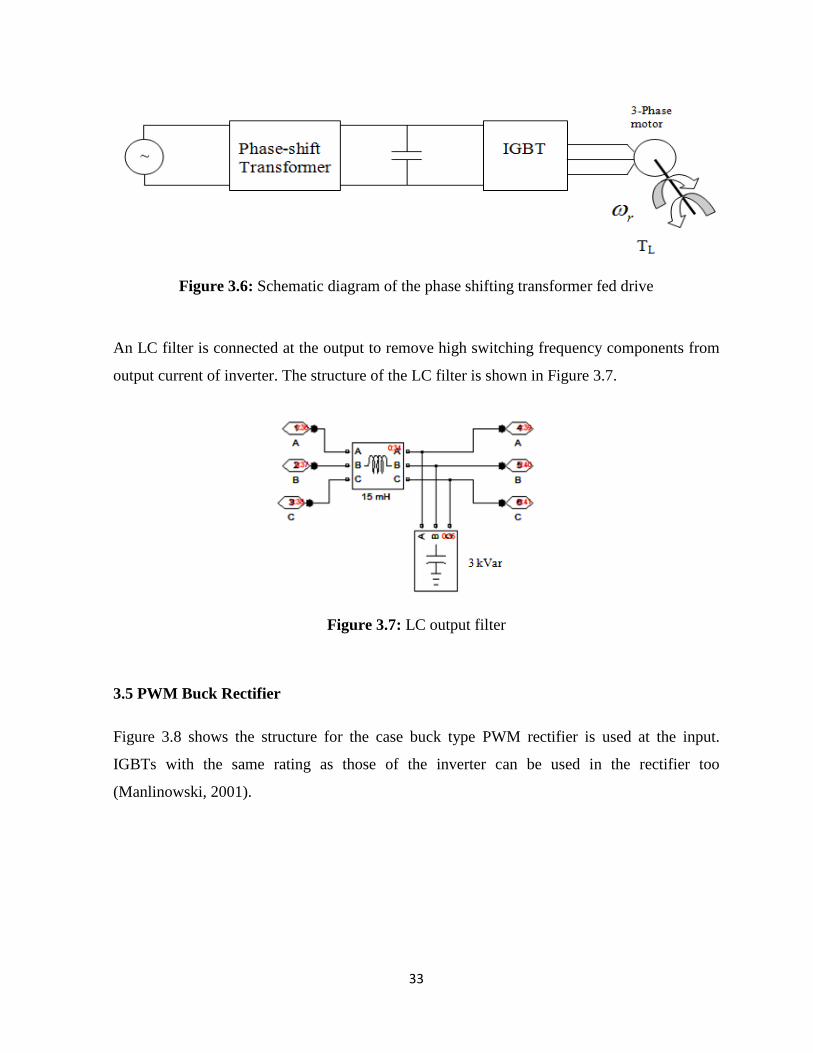
33

Figure 3.6: Schematic diagram of the phase shifting transformer fed drive

An LC filter is connected at the output to remove high switching frequency components from

output current of inverter. The structure of the LC filter is shown in Figure 3.7.

Figure 3.7: LC output filter

3.5 PWM Buck Rectifier

Figure 3.8 shows the structure for the case buck type PWM rectifier is used at the input.

IGBTs with the same rating as those of the inverter can be used in the rectifier too

(Manlinowski, 2001).

34

Figure 3.8: Schematic diagram of the PWM rectifier fed drive

35

CHAPTER 4

SIMULATION, RESULTS AND DISCUSSIONS

In this chapter, simulation results are presented for the variable frequency drive. Simulations

were performed for three cases: 1) DC bus obtained with simple diode rectifier, 2) DC bus is

obtained with PWM rectifier and 3) DC bus is obtained with phase shifting transformers (24-

pulse rectifier). Simulations were performed in Matlab R2013a Simulink program with a 4 kW

induction motor with the following parameters:

5.4 HP, 400 Volts, 50 Hz, 4-pole, 1430 rpm Induction motor.

For each type of rectifier simulation has been run for the following cases:

A. Rated load and rated speed

B. Rated load and 50% of rated speed

C. Rated load and 10% of rated speed

D. 50% of the rated load and rated speed

E. 10% of the rated load and rated speed

The devices suitable for a 4 kW system at 400 dc bus voltage have an on-state resistance of

0.001Ω. PWM gate pulses are applied to the switches of the converter. The control signal

frequency (fc) is taken as 50 Hz and the carrier frequency as 1000 Hz. Modulation index is 1.

LC filter connected to the output has the following parameters: L= 15mH, C= 66µF. Also, a 1

mH line inductance was used for each source line to represent the leakage effects.

4.1 Loading and Driving Motor

Rated power (PR) of the Variable Frequency Drive is equal to 4 kW and rated speed (nR) of

the motor is equal to 1430 rpm. The rated torque (TR) can be found as

36

P 4000RT = = = 26.71NmR

πωr n *R30

4.2 Simulation Model and Results of the Drive with Phase Shift Transformer

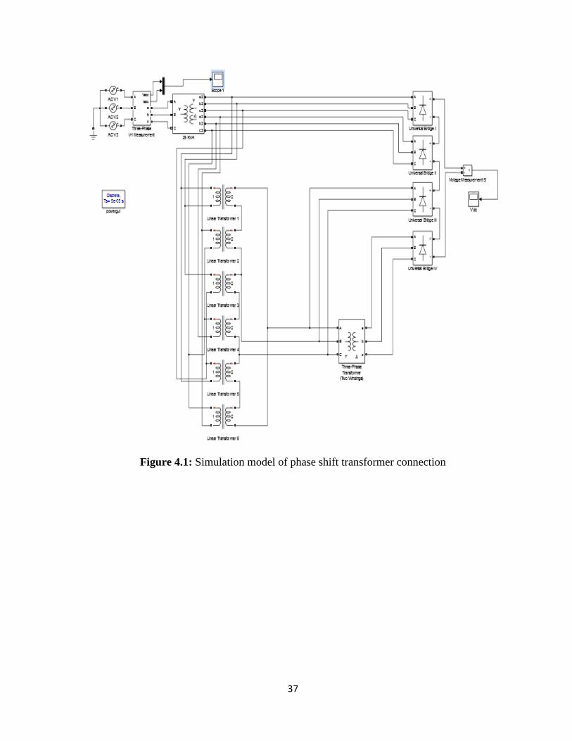
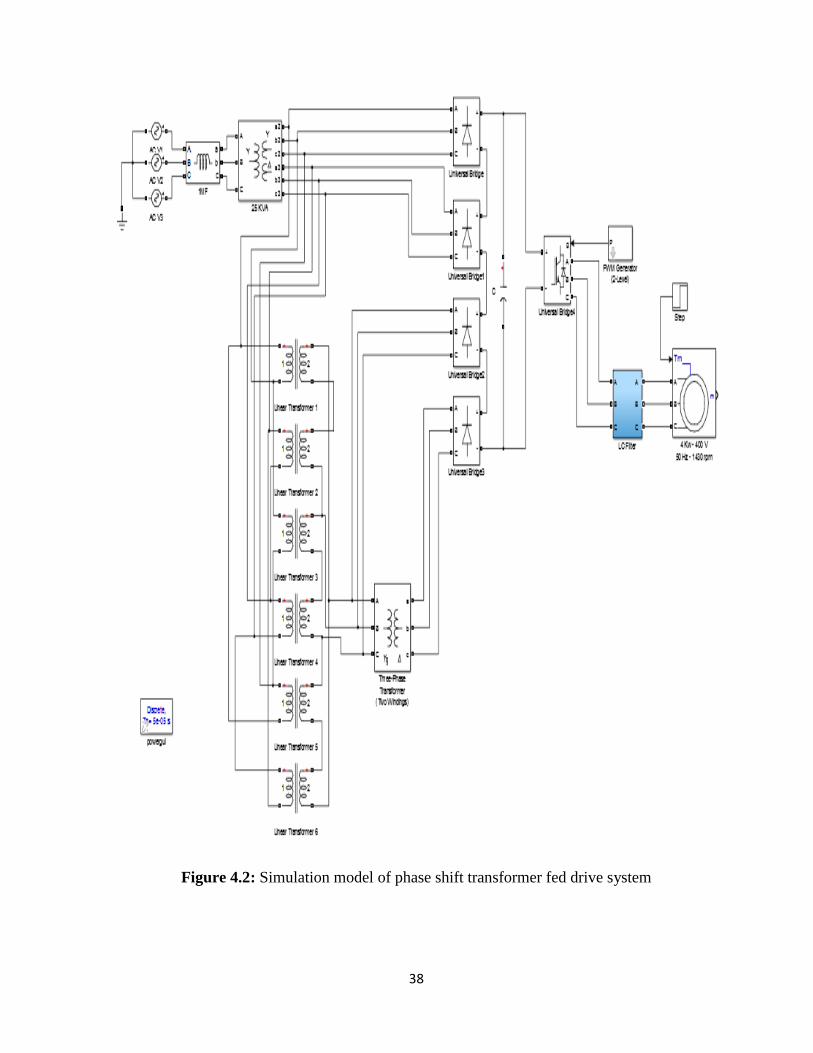
Figures 4.1 and 4.2 shows the 24-pulse rectifier that involves obtaining four individual 3-

phase systems with 15° phase shift between each output line.

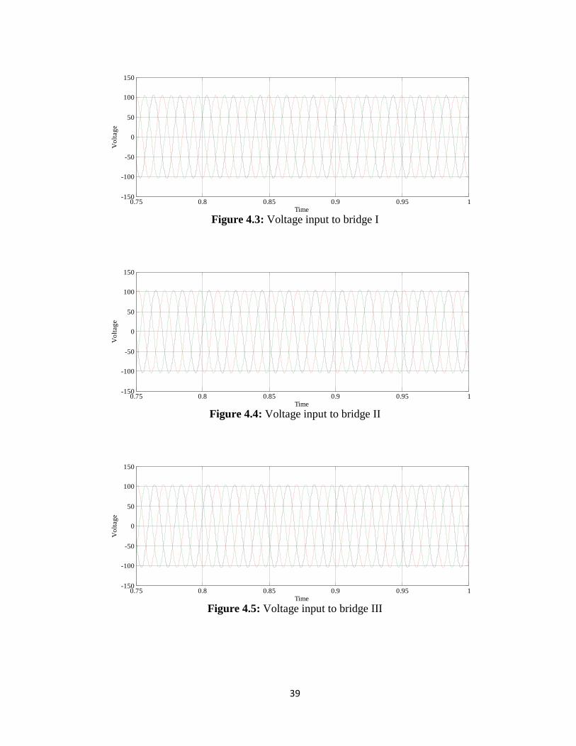
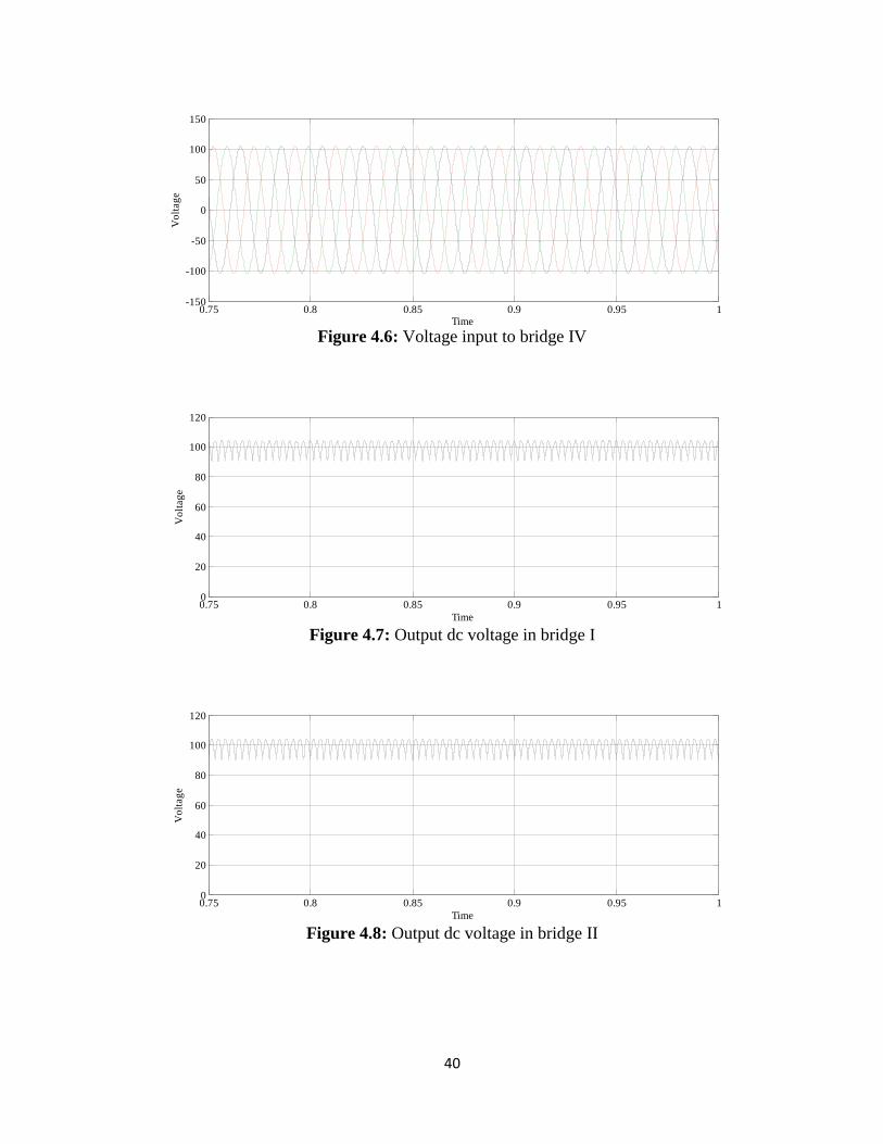
The simulation results are shown between Figure 4.3 and 4.12. Results include transformer

output voltages, rectifier output voltage, total dc link voltage, and input line voltage and

current. Power values, power factors and THD values were calculated in the simulation and

the results were summarized in Table 4.1.

37

Figure 4.1: Simulation model of phase shift transformer connection

38

Figure 4.2: Simulation model of phase shift transformer fed drive system

39

Figure 4.3: Voltage input to bridge I

Figure 4.4: Voltage input to bridge II

Figure 4.5: Voltage input to bridge III

0.75 0.8 0.85 0.9 0.95 1-150

-100

-50

0

50

100

150

Time

Vo

ltag

e

0.75 0.8 0.85 0.9 0.95 1-150

-100

-50

0

50

100

150

Time

Vo

ltag

e

0.75 0.8 0.85 0.9 0.95 1-150

-100

-50

0

50

100

150

Time

Vo

ltag

e

40

Figure 4.6: Voltage input to bridge IV

Figure 4.7: Output dc voltage in bridge I

Figure 4.8: Output dc voltage in bridge II

0.75 0.8 0.85 0.9 0.95 1-150

-100

-50

0

50

100

150

Time

Vo

ltag

e

0.75 0.8 0.85 0.9 0.95 10

20

40

60

80

100

120

Time

Vo

ltag

e

0.75 0.8 0.85 0.9 0.95 10

20

40

60

80

100

120

Time

Vo

ltag

e

41

Figure 4.9: Output dc voltage in bridge III

Figure 4.10: Output dc voltage in bridge IV

Figure 4.11: DC output voltage with series cascaded bridges (I,II,III,IV)

0.75 0.8 0.85 0.9 0.95 10

20

40

60

80

100

120

Time

Vo

ltag

e

0.75 0.8 0.85 0.9 0.95 10

20

40

60

80

100

120

Time

Vo

ltag

e

0.75 0.8 0.85 0.9 0.95 10

50

100

150

200

250

300

350

400

450

Time

Vo

ltag

e

42

Figure 4.12: 3-Phase line voltage & line current in Y winding of Yy0d1 main transformer

Table 4.1: THDI, Pf results with various cases by using phase shift transformer technique

VFD = 4 kW (5.4HP), 400V, 50Hz, 1430RPM

Case TR nR THDI pf

A (TR)

= 26.71 Nm

(nR)

= 1430 rpm

THDI

= 2.464%

pf = pf (disp)pf (dist)

= 0.965*0.999=0.96

B (TR)

= 26.71 Nm

(nR)/2

= 715 rpm

THDI

= 2.387%

pf = pf (disp)pf (dist)

= 0.97*0.99=0.97

C (TR)

= 26.71 Nm

(nR)/10

= 143 rpm

THDI

= 2.154%

pf = pf (disp)pf (dist)

= 0.97*0.99=0.97

D (TR)/2

= 13.355 Nm

(nR)

= 1430 rpm

THDI

= 2.29%

pf = pf (disp)pf (dist)

= 0.97*0.99=0.97

E (TR)/10

= 2.671 Nm

(nR)

= 1430 rpm

THDI

= 1.4%

pf = pf (disp)pf (dist)

= 0.98*0.99=0.98

4.3 Advantages of 24-Pulse Phase Shift Transformer

Virtually guarantees compliance with IEEE 519-1992.

Harmonic cancellation from the 5th to 19th

harmonics.

High power factor (0.96 -0.98).

0.75 0.8 0.85 0.9 0.95 1-400

-200

0

200

400

Time

Voltage &

Curr

ent

43

4.4 Disadvantages of 24-Pulse Phase Shift Transformer

Can be more expensive than other methods (for up to three times the harmonic

reduction of buck type PWM rectifier methods).

Larger and heavier magnetic than some other methods.

Highly complicated in design and connection.

Loss in efficiency.

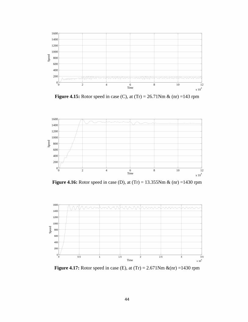
Figure 4.13: Rotor speed in case (A), at (Tr) = 26.71Nm & (nr) =1430 rpm

Figure 4.14: Rotor speed in case (B), at (Tr) = 26.71Nm & (nr) =715 rpm

0 2 4 6 8 10 12

x 104

0

200

400

600

800

1000

1200

1400

1600

Time

Sp

eed

0 2 4 6 8 10 12

x 104

0

200

400

600

800

1000

1200

1400

1600

Time

Sp

eed

44

Figure 4.15: Rotor speed in case (C), at (Tr) = 26.71Nm & (nr) =143 rpm

Figure 4.16: Rotor speed in case (D), at (Tr) = 13.355Nm & (nr) =1430 rpm

Figure 4.17: Rotor speed in case (E), at (Tr) = 2.671Nm &(nr) =1430 rpm

0 2 4 6 8 10 12

x 104

0

200

400

600

800

1000

1200

1400

1600

Time

Sp

eed

0 2 4 6 8 10 12

x 104

0

200

400

600

800

1000

1200

1400

1600

Time

Sp

eed

0 0.5 1 1.5 2 2.5 3 3.5

x 104

0

200

400

600

800

1000

1200

1400

1600

Time

Sp

eed

45

Figure 4.18: Rotor & stator current in cases (A), at (Tr) = 26.71Nm & (nr) = 1430 rpm

Figure 4.19: Rotor & stator current in cases (B), at (Tr) = 26.71Nm & (nr) = 715 rpm

Figure 4.20: Rotor & stator current in cases (C), at (Tr) = 26.71Nm & (nr) = 143 rpm

0 2 4 6 8 10 12

x 104

-50

0

50

Cu

rren

t

Ir (A)

0 2 4 6 8 10 12

x 104

-50

0

50

Time

Cu

rren

t

Is (A)

0 2 4 6 8 10 12

x 104

-50

0

50

Cu

rren

t

Ir(A)

0 2 4 6 8 10 12

x 104

-50

0

50

Time

Cu

rren

t

Is (A)

0 2 4 6 8 10 12

x 104

-20

0

20

Cu

rren

t

Ir (A)

0 2 4 6 8 10 12

x 104

-100

0

100

Time

Cu

rren

t

Is (A)

46

Figure 4.21: Rotor & stator current in cases (D), at (Tr) = 13.355Nm & (nr) = 1430 rpm

Figure 4.22: Rotor & stator current in cases (E), At (Tr) = 2.671Nm & (nr) = 1430 rpm

4.5 Simulation Results with Buck Type PWM Rectifier

The MATLAB simulation model is shown in Figure 4.8. In this model sinusoidal Pulse Width

Modulation is using to mitigate the harmonics. 340 volts, 3- phase source is used for supply

source. The buck type PWM rectifier is used to convert AC to DC and inverter is used for DC

to AC.

0 2 4 6 8 10 12

x 104

-50

0

50

Cu

rren

t

Ir (A)

0 2 4 6 8 10 12

x 104

-50

0

50

Time

Cu

rren

t

Is (A)

0 2 4 6 8 10 12

x 104

-50

0

50

Cu

rren

t

Ir (A)

0 2 4 6 8 10 12

x 104

-50

0

50

Time

Cu

rren

t

Is (A)

47

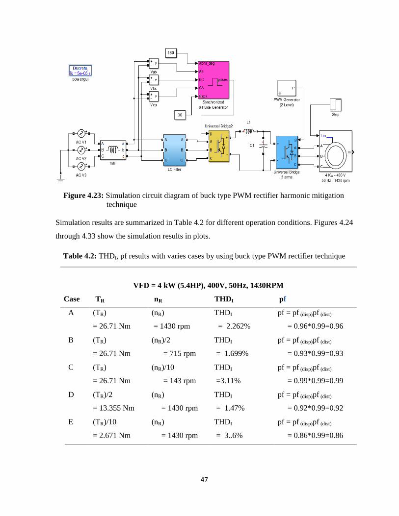
Figure 4.23: Simulation circuit diagram of buck type PWM rectifier harmonic mitigation

technique

Simulation results are summarized in Table 4.2 for different operation conditions. Figures 4.24

through 4.33 show the simulation results in plots.

Table 4.2: THDI, pf results with varies cases by using buck type PWM rectifier technique

VFD = 4 kW (5.4HP), 400V, 50Hz, 1430RPM

Case TR nR THDI pf

A (TR)

= 26.71 Nm

(nR)

= 1430 rpm

THDI

= 2.262%

pf = pf (disp)pf (dist)

= 0.96*0.99=0.96

B (TR)

= 26.71 Nm

(nR)/2

= 715 rpm

THDI

= 1.699%

pf = pf (disp)pf (dist)

= 0.93*0.99=0.93

C (TR)

= 26.71 Nm

(nR)/10

= 143 rpm

THDI

=3.11%

pf = pf (disp)pf (dist)

= 0.99*0.99=0.99

D (TR)/2

= 13.355 Nm

(nR)

= 1430 rpm

THDI

= 1.47%

pf = pf (disp)pf (dist)

= 0.92*0.99=0.92

E (TR)/10

= 2.671 Nm

(nR)

= 1430 rpm

THDI

= 3..6%

pf = pf (disp)pf (dist)

= 0.86*0.99=0.86

48

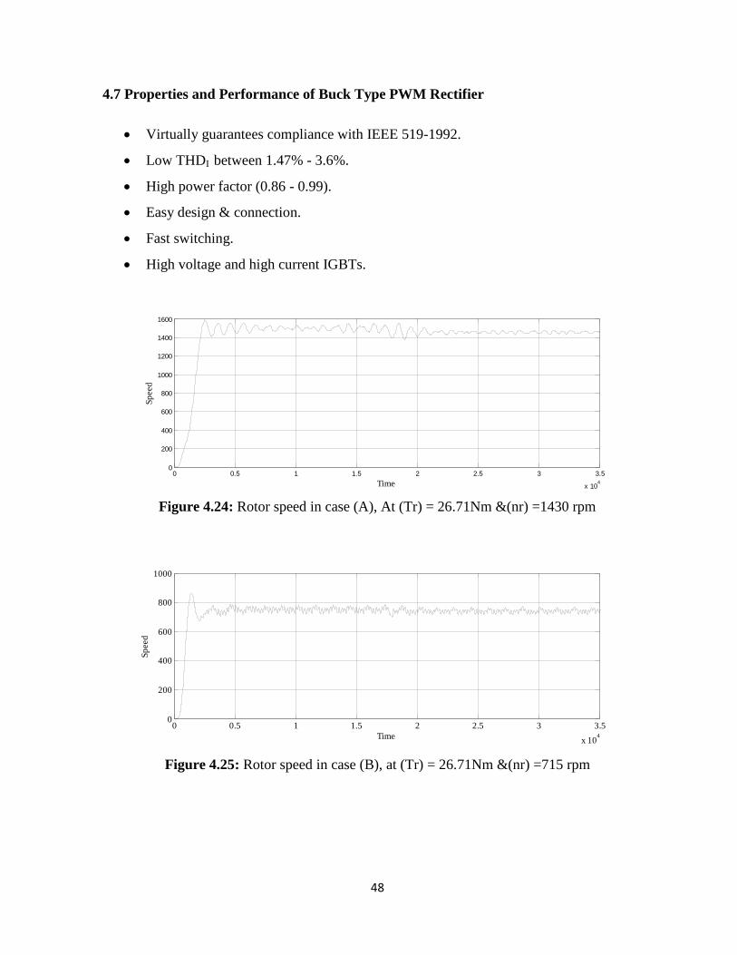
4.7 Properties and Performance of Buck Type PWM Rectifier

Virtually guarantees compliance with IEEE 519-1992.

Low THDI between 1.47% - 3.6%.

High power factor (0.86 - 0.99).

Easy design & connection.

Fast switching.

High voltage and high current IGBTs.

Figure 4.24: Rotor speed in case (A), At (Tr) = 26.71Nm &(nr) =1430 rpm

Figure 4.25: Rotor speed in case (B), at (Tr) = 26.71Nm &(nr) =715 rpm

0 0.5 1 1.5 2 2.5 3 3.5

x 104

0

200

400

600

800

1000

1200

1400

1600

Time

Sp

eed

0 0.5 1 1.5 2 2.5 3 3.5

x 104

0

200

400

600

800

1000

Time

Sp

eed

49

Figure 4.26: Rotor speed in case (C), At (Tr) = 26.71Nm & (nr) =143 rpm

Figure 4.27: Rotor speed in case (D), at (Tr) = 13.355Nm & (nr) =1430 rpm

Figure 4.28: Rotor speed in case (E), at (Tr) = 2.671Nm & (nr) =1430 rpm

0 0.5 1 1.5 2 2.5 3 3.5

x 104

0

50

100

150

200

Time

Sp

eesd

0 0.5 1 1.5 2 2.5 3 3.5

x 104

-200

0

200

400

600

800

1000

1200

1400

1600

Time

Sp

eed

0 0.5 1 1.5 2 2.5 3 3.5

x 104

0

200

400

600

800

1000

1200

1400

1600

Time

Sp

eed

50

Figure 4.29: Rotor & stator current in cases (A), At (Tr) = 26.71Nm & (nr) = 1430 rpm

Figure 4.30: Rotor & stator current in cases (B), At (Tr) = 26.71Nm & (nr) = 715 rpm

Figure 4.31: Rotor & stator current in cases (C), At (Tr) = 26.71Nm & (nr) = 143 rpm

0 0.5 1 1.5 2 2.5 3 3.5

x 104

-50

0

50

Cu

rren

t

Ir (A)

0 0.5 1 1.5 2 2.5 3 3.5

x 104

-50

0

50

Time

Cu

rren

t

Is (A)

0 0.5 1 1.5 2 2.5 3 3.5

x 104

-40

-20

0

20

Cu

rren

t

Ir (A)

0 0.5 1 1.5 2 2.5 3 3.5

x 104

-50

0

50

Time

Cu

rren

t

is (A)

0 0.5 1 1.5 2 2.5 3 3.5

x 104

-40

-20

0

20

Cu

rren

t

Ir (A)

0 0.5 1 1.5 2 2.5 3 3.5

x 104

-100

0

100

Time

Cu

rren

t

Is (A)

51

Figure 4.32: Rotor & stator current in cases (D), At (Tr) = 13.355 Nm & (nr) = 1430 rpm

Figure 4.33: Rotor & stator current in cases (E), At (Tr) = 2.671 Nm & (nr) = 1430 rpm

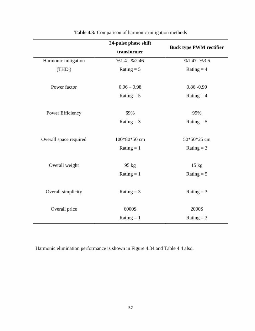
Table 4.3 gives a comparison of the two systems in terms of THD, pf, efficiency, overall

system size, overall system weight, simplicity and cost for a 4 kW system. A grade is assigned

for each criteria between 1 and 5, 5 being the best.

0 0.5 1 1.5 2 2.5 3 3.5

x 104

-50

0

50

Cu

rren

t

Ir (A)

0 0.5 1 1.5 2 2.5 3 3.5

x 104

-50

0

50

Time

Cu

rren

t

Is (A)

0 0.5 1 1.5 2 2.5 3 3.5

x 104

-50

0

50

Cu

rren

t

Ir (A)

0 0.5 1 1.5 2 2.5 3 3.5

x 104

-50

0

50

Time

Cu

rren

t

Is (A)

52

Table 4.3: Comparison of harmonic mitigation methods

24-pulse phase shift

transformer Buck type PWM rectifier

Harmonic mitigation

(THDI)

%1.4 - %2.46

Rating = 5

%1.47 -%3.6

Rating = 4

Power factor 0.96 – 0.98

Rating = 5

0.86 -0.99

Rating = 4

Power Efficiency 69%

Rating = 3

95%

Rating = 5

Overall space required

100*80*50 cm

Rating = 1

50*50*25 cm

Rating = 3

Overall weight

95 kg

Rating = 1

15 kg

Rating = 5

Overall simplicity

Rating = 3 Rating = 3

Overall price

6000$

Rating = 1

2000$

Rating = 3

Harmonic elimination performance is shown in Figure 4.34 and Table 4.4 also.

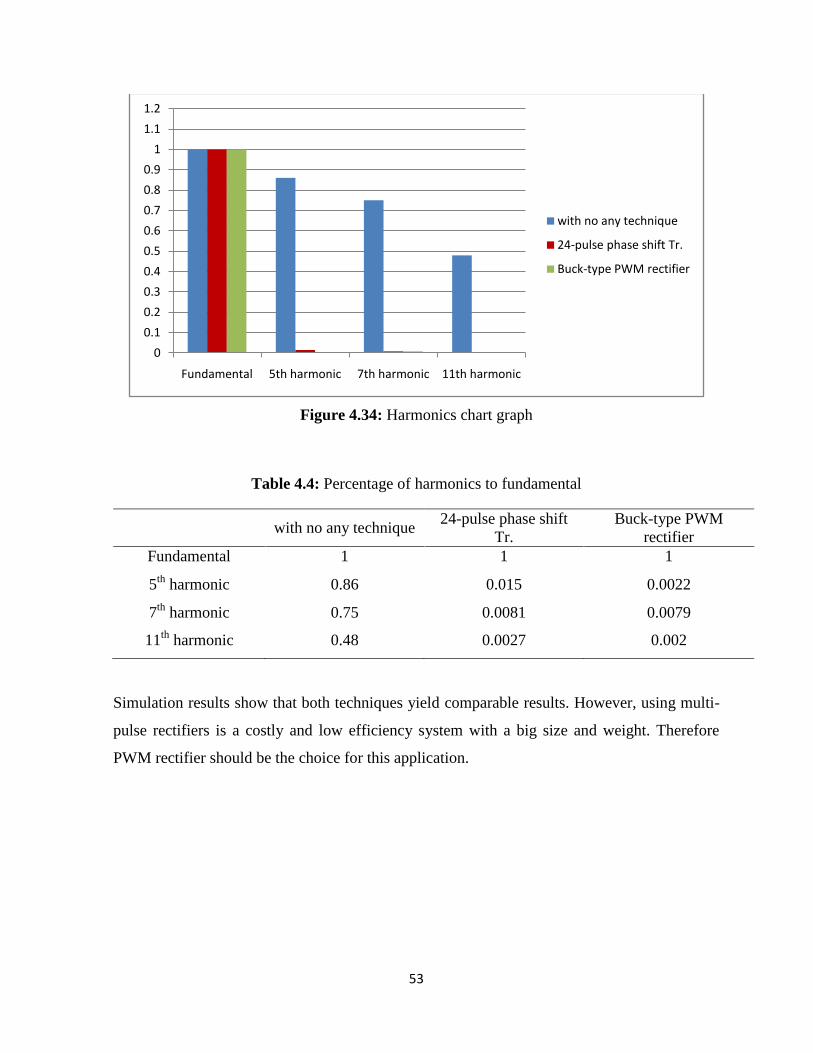
53

Figure 4.34: Harmonics chart graph

Table 4.4: Percentage of harmonics to fundamental

with no any technique

24-pulse phase shift

Tr.

Buck-type PWM

rectifier

Fundamental 1 1 1

5th

harmonic 0.86 0.015 0.0022

7th

harmonic 0.75 0.0081 0.0079

11th

harmonic 0.48 0.0027 0.002

Simulation results show that both techniques yield comparable results. However, using multi-

pulse rectifiers is a costly and low efficiency system with a big size and weight. Therefore

PWM rectifier should be the choice for this application.

0

0.1

0.2

0.3

0.4

0.5

0.6

0.7

0.8

0.9

1

1.1

1.2

Fundamental 5th harmonic 7th harmonic 11th harmonic

with no any technique

24-pulse phase shift Tr.

Buck-type PWM rectifier

54

CHAPTER 5

CONCLUSION AND SUGGESTIONS FOR FUTURE WORK

5.1 Conclusion

The front end rectifier used in VFDs is a big source of harmonics. In this thesis, two different

front-end rectifier topologies have been used and compared through simulations under various

operation conditions.

One of the techniques is using a multi-pulse rectifier. A 24-pulse rectifier has been designed

and tested by simulation. The turns ratios and connection diagrams of the phase shift

transformers are given.

The second technique used in this thesis is PWM rectifier. This rectifier has also been

simulated under the same conditions.

Simulations have been carried out in MATLAB Simulink R2013a. The following points are

observed:

Nowadays, harmonic distortions and low Power Factor (pf) are serious problems that

gained more importance in VFD as a power electronics area. Harmonic mitigation and

power factor correction can be achieved by using a 24-pulse phase shift transformer

and buck type PWM rectifier.

Harmonic mitigation and power factor correction can be achieved by using a 24-pulse

phase shift transformer and buck type PWM rectifier.

A 24-pulse phase shift transformer rectifier achieved by conversion of a 3-phase

voltage source power supply to four individual 3-phase isolated systems by utilized a

novel interconnection of conventional 3-phase, and single phase transformer. The

transformers are used for creating the relevant phase shifting (15°). The 24-pulse

output dc voltage results by cascading of four six-pulse diode bridges that are sustained

by the four individual isolated 3-phase voltage.

55

Mitigation harmonic circuit with 24-pulse phase shift transformer topology controls the

THD and input power factor correction very much better than the circuit buck type

PWM rectifier technique. The THDI reduced to 2.73% and the power factor improved

to a value 0.965. So 24-pulse phase shift transformer technique topology can be

considered as a good choice for harmonic mitigation and improving of power factor.

Pulse Width Modulation (PWM) rectifier in distribution systems represents the best

solution if compared the results of both techniques as a base of cost & size. The

simulation and the results based on PWM rectifier AC-DC converter has improved

efficiency and, high dynamic performance and has distortion well under (5%) which is

quite acceptable in IEEE 519-1992 recommended.

5.2 Future Work

Further research can be done in the following areas:

Study of (delta-polygon) connected transformer-based 36-pulse (ac to dc) converter for

improvement power quality.

Comparative analysis of 36, 48, 60 pulse AC-DC controlled multi-pulse converters for

Harmonic Mitigation.

Advanced control techniques on PWM rectifiers to improve the THD.

56

REFERENCES

Abanihi, K. V., Aigbodion, D. O., Kokoette, E. D., & Samuel, D. R. (2014). Analysis of load

test, transformation, turns ratio, Efficiency and voltage regulation of single Phase

transformer. International Journal of Science, Environment, and Technology, 3(5),

3411-3414.

Akter, M. P., Mekhilef, S., Tan, N. M. L., & Akagi, H. (2015). Stability and performance

investigations of model predictive controlled active-front-end (AFE) rectifiers for

energy storage systems. Journal of Power Electronics, 15(1), 202-215.

Arvindan, A. N. (2010, October). 24-pulse rectifier topology with 3-phase to four 3-phase

transformation by novel interconnection of conventional 3-phase and 1-phase

transformers. In IPEC, 2010 Conference Proceedings (pp. 973-979). IEEE.

BalaRaju, U. P., Kethineni, B., Shewale, R., & Grourishetti, S. (2012). Harmonic Effects and

Its Mitigation Techniques for a Nonlinear Load. International Journal of Advanced

Technology & Engineering Research, 2, 122-127.

Bhattacharya, M. (2014). Improvement of Power Quality Using PWM Rectifiers.

International Journal of Scientific and Research Publications, 4(7), from

http://www.ijsrp.org/research-paper-0714/ijsrp-p3178.pdf

Duffey, C. K., & Stratford, R. P. (1989). Update of harmonic standard IEEE-519: IEEE

recommended practices and requirements for harmonic control in electric power

systems. IEEE Transactions on Industry Applications, 25(6), 1025-1034.

Khan, M. Z., Naveed, M. M., & Hussain, D. A. (2013). Three phase six-switch PWM buck

rectifier with power factor improvement. In Journal of Physics: Conference Series

(Vol. 439, No. 1, p. 012028). IOP Publishing.

Kiessling, F., Puschmann, R., Schmieder, A., & Schneider, E. (2009). Contact Lines for

Electric Railways. Planning, Design, Implementation, Maintenance.

57

Malinowski, M. (2001). Sensorless control strategies for three-phase PWM rectifiers.

Rozprawa doktorska, Politechnika Warszawska, Warszawa.

Sandoval, G. (2014). Power Factor in Electrical Power Systems with Non-Linear Loads.

ARTECHE/INELAP, from

http://www.apqpower.com/assets/files/PF_nonlinearloads.pdf

Sapin, A., Allenbach, P., & Simond, J. J. (2000). Modeling of Multi-winding Phase Shifting

Transformers: Application to DC and Multi-level VSI Supplies. In PCIM Highlights of

the fourteenth International Conference on Electrical Machines, (Vol. 6, No. LME-

CONF-2009-009), from

https://infoscience.epfl.ch/record/133173/files/PCIM_momwpstatdamlvs

Singh, A., & Jabir, V. S. (2014). Voltage Fed Full Bridge DC-DC and DC-AC Converter for

High-Frequency Inverter Using C2000. Texas Instruments Application Report, from

http://www.ti.com/lit/an/sprabw0b/sprabw0b.pdf

Svensson, S. (1999). Power measurement techniques for nonsinusoidal conditions. The

significance of harmonics for the measurement of power and other AC quantities.

Chalmers University of Technology, from

https://www.sp.se/en/index/services/DSWM/Documents/SvenssonStefanPhD.pdf

Wang, X., Huang, K., Yan, S., & Xu, B. (2008, May). Simulation of three-phase voltage

source PWM rectifier based on direct current control. In Image and Signal Processing,

2008. CISP'08. Congress on (Vol. 5, pp. 194-198), from

http://ieeexplore.ieee.org/stamp/stamp.jsp?tp=&arnumber=4566815

Wu, B. (2006). High-power converters and AC drives. John Wiley & Sons, from

https://www.researchgate.net/publication/255702339_HighPower_Converters_and_

AC_Drivesfull

58

APPENDECES

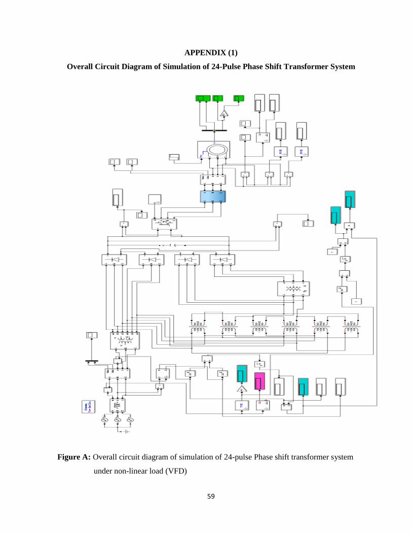
59

APPENDIX (1)

Overall Circuit Diagram of Simulation of 24-Pulse Phase Shift Transformer System

Figure A: Overall circuit diagram of simulation of 24-pulse Phase shift transformer system

under non-linear load (VFD)

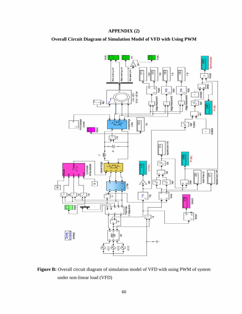
60

APPENDIX (2)

Overall Circuit Diagram of Simulation Model of VFD with Using PWM

Figure B: Overall circuit diagram of simulation model of VFD with using PWM of system

under non-linear load (VFD)

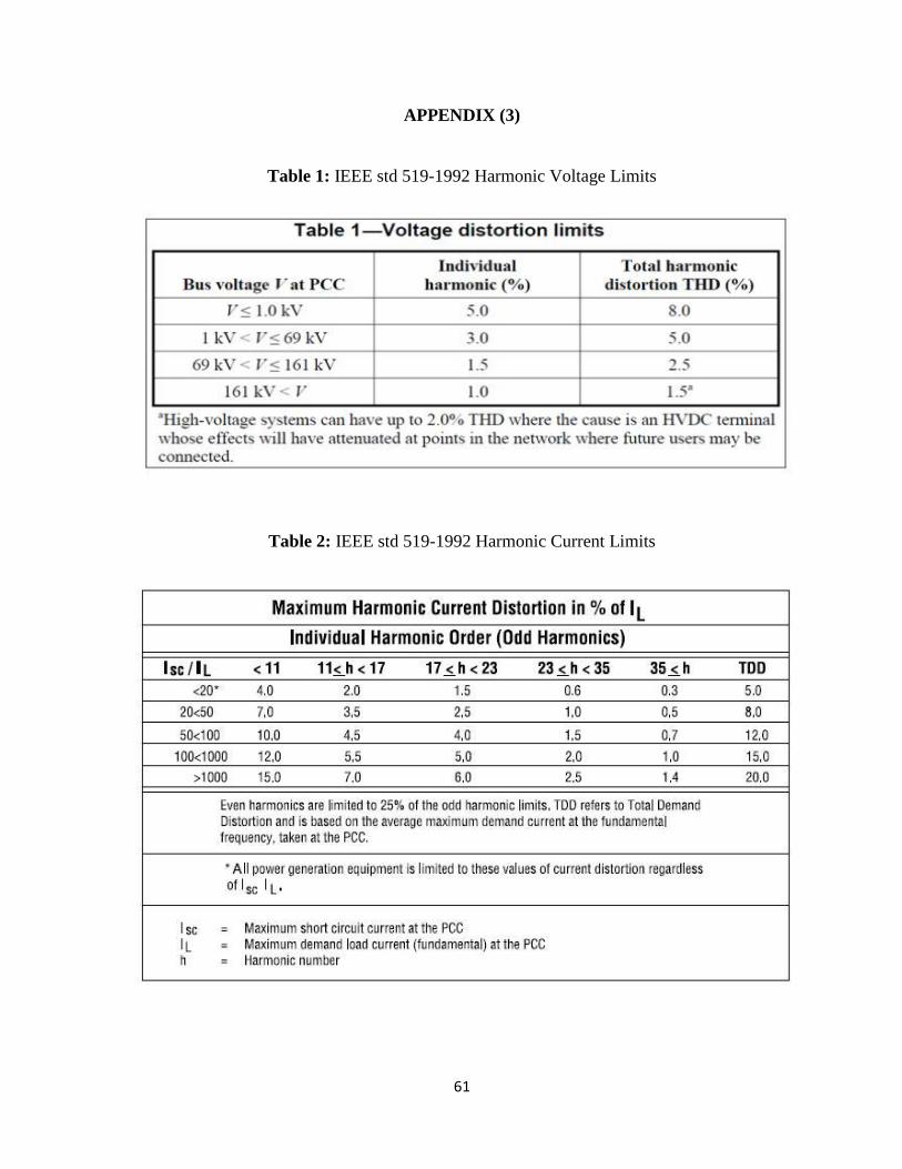
61

APPENDIX (3)

Table 1: IEEE std 519-1992 Harmonic Voltage Limits

Table 2: IEEE std 519-1992 Harmonic Current Limits

62

Table 3: IEEE std 519-1992, listing recommended harmonic voltage limits

Harmonic Voltage Limits

(low-voltage system)

Application Maximum THD (%)

Special applications ----- Hospitals and airports 3.0

General system 5.0

Dedicated system ----- exclusively converter load 10.0