Effect of Turbulence Model on the Calculated Flowthrough Rectilinear Turbine Cascade

By Mahmoud M. El-GENDI1) and Mohammed K. IBRAHIM2)

1)Mechanical Power and Energy Department, Faculty of Engineering, Minia University, Minia,Egypt

2)Aerospace Engineering Department, Faculty of Engineering, University of Cairo, Giza, Egypt

Flow simulations through a turbine cascade were carried out for an exit isentropic Mach

number of 0.6 and a Reynolds number of 1.6 × 105. The main objective of the present study is to

study the effect of turbulence model on the calculated results. Calculations were carried out using

a locally developed numerical code, where a 2nd order Roe’s flux-difference splitting for inviscid

numerical fluxes and a 2nd order implicit dual time method for time integration. Three turbulence

models were compared namely SpalartAllmaras, Delayed Detached Eddy Simulation and Improved

Delayed Detached Eddy Simulation. In addition, the results of laminar calculation was considered.

The results show that although the turbulence models damped the flow unsteadiness, they have

good agreement with experimental results than laminar calculation.

Keywords: Gas Turbines, CFD, Turbulence model

1. Introduction

Due to the importance of the low pressure (LP) turbines, many researchers investigated T106LP turbine cascade. Stieger1) carried out pressure measurements on the suction side. There is amoving bar wake generator passing in front of this cascade. On the other hand, Suzen and Huang2)

carried out numerical simulations using an intermittency transport equation. Langtry3) proposed acorrelation based on transition model. Stieger4) carried out measurement as a data base for CFDvalidation. In the present work, a comparison among three turbulence models in addition to laminarcalculation were carried out on the same LP turbine cascade (T 106).

2. Investigated cascade

The investigated cascade is a T 106 LP turbine cascade. It has a chord of 198 mm, axial chordof 170 mm, a blade stagger angle of 30.7◦, a pitch of 158 mm, and the inlet flow angle is 37.7◦. Theblade co-ordinates can be found in Stieger4).

3. Numerical method

3.1. Computational grid

The H-type grid was used in all cases. The grid has 402 points in the stream-wise direction, 210points in the pitch direction, and 3 points in the span direction; total number of grid points is about2.53×105.

1

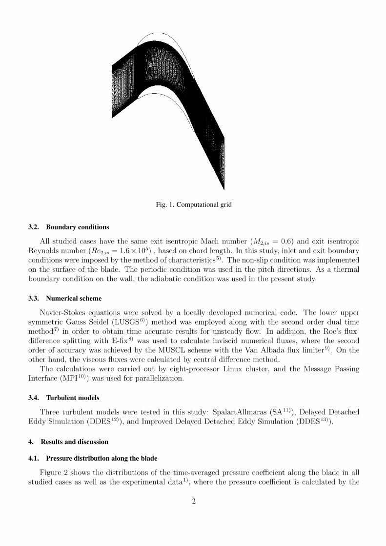
Fig. 1. Computational grid

3.2. Boundary conditions

All studied cases have the same exit isentropic Mach number (M2,is = 0.6) and exit isentropicReynolds number (Re2,is = 1.6×105) , based on chord length. In this study, inlet and exit boundaryconditions were imposed by the method of characteristics5). The non-slip condition was implementedon the surface of the blade. The periodic condition was used in the pitch directions. As a thermalboundary condition on the wall, the adiabatic condition was used in the present study.

3.3. Numerical scheme

Navier-Stokes equations were solved by a locally developed numerical code. The lower uppersymmetric Gauss Seidel (LUSGS6)) method was employed along with the second order dual timemethod7) in order to obtain time accurate results for unsteady flow. In addition, the Roe’s flux-difference splitting with E-fix8) was used to calculate inviscid numerical fluxes, where the secondorder of accuracy was achieved by the MUSCL scheme with the Van Albada flux limiter9). On theother hand, the viscous fluxes were calculated by central difference method.

The calculations were carried out by eight-processor Linux cluster, and the Message PassingInterface (MPI10)) was used for parallelization.

3.4. Turbulent models

Three turbulent models were tested in this study: SpalartAllmaras (SA11)), Delayed DetachedEddy Simulation (DDES12)), and Improved Delayed Detached Eddy Simulation (DDES13)).

4. Results and discussion

4.1. Pressure distribution along the blade

Figure 2 shows the distributions of the time-averaged pressure coefficient along the blade in allstudied cases as well as the experimental data1), where the pressure coefficient is calculated by the

2

s/s0

cp

0 0.2 0.4 0.6 0.8 10

0.2

0.4

0.6

0.8

1

1.2

1.4

1.6

Experiment

Laminar

SA

DEES

IDDES

Fig. 2. Pressure coefficient along blade surface; Experiment was carried out by Stieger et al.1)

following equation:Cp = (P0 − P )/(P0 − P2) (1)

where, P0, is total pressure at the inlet, and P2, is pressure at the exit. In all studied cases, thenumerical results show good agreement with that of the experimental data1) along the pressure side.Along the suction side, there are deviation until S/S0 ≈ 0.5. From S/S0 ≈ 0.5, all turbulent calcu-lations show good agreement with with that of the experimental data1), but the laminar calculationhas a deviation.

4.2. Pressure contours

The time-averaged dimensionless pressure contours through the cascade are shown in Fig. 3 forall studied cases. As shown in Fig. 3 for all cases, the pressure has high value near the pressure sideand decreases gradually toward the suction side. In the wake region, the effect of the vortex sheddingis much clearer in the laminar calculation than all turbulent calculations.

4.3. Vorticity

The instantaneous dimensionless vorticity contours through the cascade are shown in Fig. 4 forall studied cases. As shown in Fig. 4 for all cases, the vorticity has a distinctive value near the bladeand in the wake region. The turbulent calculations damped the flow unsteadiness, but the effect ofthe vortex shedding is clear in the laminar calculation.

3

(a) SA (b) DDES

(c) IDDES (d) Laminar

Fig. 3. Dimensionless pressure contours

4

(a) SA (b) DDES

(c) IDDES (d) Laminar

Fig. 4. Dimensionless vorticity

5

(a) SA (b) DDES

(c) IDDES

Fig. 5. Dimensionless eddy viscosity

4.4. Eddy viscosity

Figure 5 shows the contours of the dimensionless eddy viscosity for all turbulent calculations.The eddy viscosity has a distinctive value near the suction side of the rear of the blade and in thewake region. The eddy viscosity has higher value in the case of SA than DDES, and it has highervalue in the case of DDES than IDDES.

5. Conclusion

The numerical simulation of the flow field of a turbine cascade was carried out. The effect of theturbulence model of the flow field was considered. Three turbulence models were tested in additionto laminar calculation.

The computational results showed that there are similarity among all studied cases. The SAturbulence model has the highest eddy viscosity, and IDDES turbulence model has the lowest eddyviscosity. For the pressure coefficient along the blade, the turbulent calculations have more agree-ment with experimental results1) than laminar calculation. The turbulence models damped the flowunsteadiness, and the unsteadiness effect of the vortex shedding is observed only in the laminar cal-culation.

6

References

1) R. Stieger, D. Hollis, and H. Hodson. Unsteady Surface Pressures Due to Wake Induced Transi-tion in A Laminar Separation Bubble on A LP Turbine Cascade. In Proceedings of ASME TurboExpo 2003 Power for Land, Sea and Air June 16-19, Atlanta, Georgia, USA, 2003.

2) Y. B. Suzen and P. G. Huang. Numerical Simulation of Unsteady Wake/Blade Interactionsin Low Pressure Turbine Flows using an Intermittency Transport Equation. In Proceedings ofASME Turbo Expo 2004 Power for Land, Sea, and Air June 14-17, 2004, Vienna, Austria, 2004.

3) R. B. Langtry. A Correlation-Based Transition Model using Local Variables for UnstructuredParallelized CFD Codes. PhD thesis, Institut fr Thermische Stromungsmaschinen und Maschi-nenlaboratorium Universitat Stuttgart, 2006.

4) R. D. Stieger. The Effects of Wakes on Separating Boundary Layers in Low Pressure Turbines.PhD thesis, Cambridge University Engineering Department, 2002.

5) J. Blazek. Computational Fluid Dynamics; Principles and Applications. ELSEVIER, 2001.

6) S. Yoon and A. Jameson. Lower-Upper Symmetric-Gauss-Seidel Method for the Euler andNavier-Stokes Equations. AIAA J., 26(9):1025–1026, 1988.

7) L. Dubuc, F. Cantariti, M. Woodgate, B. Gribben, K. J. Badcock, and B. E. Richards. Solutionof the Unsteady Euler Equations Using an Implicit Dual-Time Method. AIAA J., 36(8):1417–1424, 1998.

8) P. L. Roe. Approximate Riemann Solver, Parameter Vectors, and Difference Schemes. Journalof Computational Physics, 43:357–372, 1981.

9) C. Hirsch. Numerical Computation of Internal and External Flows. Engineering EducationSystem, 2000.

10) W.Gropp, E. Lusk, and A. Skjellum. Using MPI : Portable Parallel Programming with theMessage-Passing Interface. MIT press, 1999.

11) P. R. Spalart and S. R. Allmaras. A One-Equation Turbulence Model for Aerodynamic Flows.In AIAA-92-0439, 30th Aerospace Sciences Meeting and Exhibit, 1992.

12) P. R. Spalart, S. Deck, M. L. Shur, K. D. Squires, M. Kh. Strelets, and A. Travin. A NewVersion of Detached-Eddy Simulation, Resistant to Ambiguous Grid Densities. Theor. Comput.Fluid Dyn., 20:181–195, 2006.

13) M. L. Shur, P. R. Spalart, M. Kh. Strelets, and A.K. Travin. A Hybrid RANS-LES Approachwith Delayed-DES and Wall-Modelled LES Capabilities. International Journal of Heat and FluidFlow, 29:1638–1649, 2008.

7