Embed Size (px)
Citation preview

University of Nebraska - LincolnDigitalCommons@University of Nebraska - LincolnArchitectural Engineering -- Dissertations andStudent Research Architectural Engineering
5-2015
Effect of the physical environment on teachersatisfaction with indoor environmental quality inearly learning schoolsStuart ShellUniversity of Nebraska-Lincoln, [email protected]
Follow this and additional works at: http://digitalcommons.unl.edu/archengdiss
Part of the Architectural Engineering Commons, and the Industrial and OrganizationalPsychology Commons
This Article is brought to you for free and open access by the Architectural Engineering at DigitalCommons@University of Nebraska - Lincoln. It hasbeen accepted for inclusion in Architectural Engineering -- Dissertations and Student Research by an authorized administrator ofDigitalCommons@University of Nebraska - Lincoln.
Shell, Stuart, "Effect of the physical environment on teacher satisfaction with indoor environmental quality in early learning schools"(2015). Architectural Engineering -- Dissertations and Student Research. 34.http://digitalcommons.unl.edu/archengdiss/34

EFFECT OF THE PHYSICAL ENVIRONMENT ON TEACHER SATISFACTION
WITH INDOOR ENVIRONMENTAL QUALITY IN EARLY LEARNING SCHOOLS
by
Stuart Shell
A THESIS
Presented to the Faculty of
The Graduate College at the University of Nebraska
In Partial Fulfillment of Requirements
For the Degree of Master of Science
Major: Architectural Engineering
Under the Supervision of Professor Lily M. Wang
Lincoln, Nebraska
May 2015

EFFECT OF THE PHYSICAL ENVIRONMENT ON TEACHER SATISFACTION
WITH INDOOR ENVIRONMENTAL QUALITY IN EARLY LEARNING SCHOOLS
Stuart Shell, M.S.
University of Nebraska, 2015
Advisor: Lily M. Wang
While the quantity and quality of teacher-child interactions plays a key role in
emotional and cognitive development for children, there is scant evidence regarding the
contribution of physical environment to child outcomes. This study seeks to understand
better the relative importance of variables within the physical environment for occupants.
The research design targets teachers’ satisfaction with the physical environment as the
outcome variable, based on the assumption that teachers who are more satisfied with their
classroom provide higher-quality interactions with children. Teachers from two early
learning schools with a total of 31 classrooms completed a written survey that asked
about lighting, acoustics, air quality, job satisfaction and overall satisfaction with the
space. The predictor variables are measurements from each sensory domain including
illuminance, particulate matter, carbon dioxide and sound pressure level. Results suggest
that background noise, lighting and floor area are good predictors of teacher satisfaction.
Teachers’ perceptions of various sensory domains are related. Organizational satisfaction
mediates satisfaction with some features of the physical environment. Discussion
includes implications for early learning programs and the design and renovation of
classroom spaces.

iv
DEDICATION
To Dana, for the motivation to explore the genius of childhood.

v
ACKNOWLEDGEMENTS
Educare of Omaha has enabled this study by giving purpose to my inquiry and
participating as a full partner in research. The organization’s contribution to the health
and resilience of the community is my inspiration for taking a closer look at what
designers and facility managers can contribute to the loving work of supporting our
youngest learners. From teacher’s aides to the director of research, to a person, the
organization has supported this effort by taking the time to share insights and creating
space in their schedule to allow for my data collection. I am grateful to Educare of
Omaha for the trailblazing program they deliver and for supporting my study.
RDG Planning & Design has contributed resources and expertise to this project.
In addition to designing the schools included in my study, they provided troves of
information on the project and facilitated personal connections with Educare of Omaha.
By seriously investigating how buildings are actually used, the company has
demonstrated a profound commitment to its clients. I am grateful to RDG Planning &
Design for sharing with me a vision of community service and excellence in design as an
employee and a citizen architect.
I first asked Dr. Lily M. Wang in 2011 if the university could teach me to use
research as part of my work as an architect. She said “yes” and has continued to show
how much more there was to gain from the halls of the academy. Not only has she guided
me through the channels to gain a basic competency in engineering, but she is also a role
model to me for how a design professional can succeed in mentoring others while
contributing to a community of knowledge. Thank you, Dr. Wang.

vi
TABLE OF CONTENTS
Abstract ............................................................................................................................... ii
Approvals ........................................................................................................................... iii
Dedication .......................................................................................................................... iv
Acknowledgements ..............................................................................................................v
Table of Contents ............................................................................................................... vi
List of Figures ................................................................................................................... vii
List of Tables .......................................................................................................................x
CHAPTER 1 - Introduction ................................................................................................ 1
CHAPTER 2 - Literature Review ....................................................................................... 4
CHAPTER 3 - Methodology ............................................................................................ 35
CHAPTER 4 - Results ...................................................................................................... 57
CHAPTER 5 - Discussion .............................................................................................. 111
CHAPTER 6 - Summary ................................................................................................ 118
REFERENCES ............................................................................................................... 120
APPENDIX A - Predictor Variable Data ........................................................................ 132
APPENDIX B - Outcome Variable Data ........................................................................ 142
APPENDIX C - Participant Survey ................................................................................ 156

vii
LIST OF FIGURES
Figure 1-1: Framework for Program Quality and the Physical Environment .................... 2
Figure 3-1: Occupied Measurement Meters ..................................................................... 37
Figure 3-2: Typical Room Impulse Response Measurement Setup ................................. 40
Figure 4-1: Classrooms A18 & B97 Teacher Agreement ................................................ 57
Figure 4-2: Classrooms A19 & B12 Teacher Agreement ................................................ 58
Figure 4-3: Classroom B89 Teacher Response Histograms ............................................. 58
Figure 4-4: Sensory Composite Score Agreement ........................................................... 63
Figure 4-5: Size Composite Score and Area by School ................................................... 66
Figure 4-6: Area and Size Composite Score Overall and by School ............................... 67
Figure 4-7: Area and Size Composite Score by Classroom Type .................................... 69
Figure 4-8: Size Composite Score by BNL ...................................................................... 70
Figure 4-9: Size Composite Score by BNL and Classroom Type .................................... 70
Figure 4-10: View Composite Score by School and Item ieqoverall ....................... 72
Figure 4-11: View Composite Score by Illuminance Ratio ............................................. 72
Figure 4-12: Composite Acoustic Score by School and Classroom Type ....................... 73
Figure 4-13: Acoustical Measurements Distribution ....................................................... 75
Figure 4-14: Floor Area by Reverberation Time .............................................................. 76
Figure 4-15: Acoustic Composite Score by Quiet Unoccupied BNL .............................. 77
Figure 4-16: Acoustic Composite Score by Relative Humidity ....................................... 77
Figure 4-17: Item stcsat by Occupied BNL Within School ........................................ 78
Figure 4-18: Thermal Composite Score by School and Classroom Type ........................ 79
Figure 4-19: Thermal Composite Scores by Classroom Type Within School ................. 80

viii
Figure 4-20: Temperature by Classroom Type Within School ........................................ 80
Figure 4-21: Thermal Composite Score by Color and Orientation .................................. 81
Figure 4-22: Composite Air Score by School and Classroom Type ................................ 83
Figure 4-23: Particulate Matter by Classroom Type ........................................................ 84
Figure 4-24: Air Quality Measures by School ................................................................. 85
Figure 4-25: Relative Humidity by Classroom Type ....................................................... 86
Figure 4-26: Composite Air Score by CO2 Concentration (10-Hour) .............................. 87
Figure 4-27: Composite Lighting Scores by School and Classroom Type ...................... 89
Figure 4-28: Lighting Characteristics by School .............................................................. 90
Figure 4-29: Composite Lighting Score by Illuminance Ratio ........................................ 91
Figure 4-30: Natural Light Composite Score by Area Within School ............................. 92
Figure 4-31: Natural Light Composite Score by Illuminance Within School .................. 92
Figure 4-32: Natural Light Composite Score by BNL Within School ............................. 93
Figure 4-33: Natural Light Composite Score by Background Noise Delta...................... 94
Figure 4-34: Furnishings Composite Score by School ..................................................... 95
Figure 4-35: Furnishings Composite Score by Wall Color .............................................. 96
Figure 4-36: Furnishings Composite Score by Carbon Dioxide Concentration............... 96
Figure 4-37: Composite Cleaning Score by School and Classroom Type ....................... 97
Figure 4-38: Cleaning Composite Score by Wall Color .................................................. 98
Figure 4-39: Cleaning Composite Score by Illuminance ................................................. 98
Figure 4-40: Cleaning Composite Score by Reverberation Time .................................... 99
Figure 4-41: Cleaning Composite Score by Carbon Dioxide Concentration ................... 99
Figure 4-42: Score Distribution for IEQ Overall Measures ........................................... 100

ix
Figure 4-43: Item ieqoverall by IEQ Composite Scores ........................................ 101
Figure 4-44: Area by IEQ Scores Within School ........................................................... 103
Figure 4-45: Unoccupied Quiet BNL by IEQ Scores Within School ............................ 104
Figure 4-46: Unoccupied Loud BNL by Broad IEQ Score Within School .................... 105
Figure 4-47: Composite Sensory IEQ Score by Relative Humidity............................... 106
Figure 4-48: Illuminance and Illuminance Ratio by IEQ Scores Within School ........... 108
Figure 4-49: Confounds with Carpet .............................................................................. 109
APPENDICES
Figure A-1: Room A38 Measures – 22 Hours ................................................................ 136
Figure A-2: Room B24 Measures – 22 Hours ................................................................ 137
Figure A-3: Room A38 Measures – 10 Hours ................................................................ 138
Figure A-4: Room A38 Measures – 10 Hours ................................................................ 139
Figure A-5: Room A88 Particulate Matter Concentration 15-Minute TWA – Day 1 .... 140
Figure A-6: Room A88 Particulate Matter Concentration 15-Minute TWA – Day 2 .... 140
Figure A-7: Room A88 Particulate Matter Concentration 15-MinuteTWA – Day 3 ..... 140
Figure B-1: Lead Teacher Survey Data by Classroom ................................................... 142
Figure B-2: Assistant Teacher Survey Data by Classroom ............................................ 143
Figure B-3: Teacher’s Aide Survey Data by Classroom ................................................ 144
Figure B-4: Spearman’s Rank Correlation Significance for Survey Items .................... 145

x
LIST OF TABLES
Table 3-1: Measurement Equipment ................................................................................. 39
Table 3-2: Predictor Variables in the Physical Environment ........................................... 44
Table 3-3: Survey Response Items .................................................................................... 48
Table 3-4: Participant Characteristics by Classroom Type ............................................. 51
Table 3-5: Participant Characteristics by School ............................................................ 52
Table 3-6: Study Hypotheses ............................................................................................. 56
Table 4-1: Composite Scores and Constituent Items ........................................................ 61
Table 4-2: Composite Score Pearson’s Correlations ....................................................... 62
Table 4-3: Composite Score Spearman’s Correlations .................................................... 64
Table 4-4: Pearson’s Correlations of Organizational Satisfaction Items ........................ 65
Table 4-5: Pearson’s Correlations of Size Items .............................................................. 66
Table 4-6: Pearson’s Correlations of View Items............................................................. 71
Table 4-7: Pearson’s Correlations of Acoustic Outcome Variables ................................ 73
Table 4-8: Pearson’s Correlations of Thermal Outcome Variables ................................. 79
Table 4-9: Pearson’s Correlations for Air Quality Outcome Items ................................. 82
Table 4-10: Pearson’s Correlations of Lighting Outcome Items...................................... 88
Table 4-11: Pearson’s Correlations of Furniture Outcome Items.................................... 95
Table 4-12: Pearson’s Correlations of Cleaning Outcome Items .................................... 97
Table 4-13: Pearson’s Correlation of IEQ Scores ......................................................... 101
Table 4-14: Composite Score Summary .......................................................................... 110
Table 5-1: Coefficient Comparison for IEQ Overall ...................................................... 115

xi
APPENDICES
Table A-1: Observational Measures ............................................................................... 132
Table A-2: Classroom Air Quality and Thermal Comfort Measures ............................. 133
Table A-3: Classroom Acoustical Measures .................................................................. 134
Table A-4: Classroom Lighting Measures ...................................................................... 135
Table A-5: Example of Observational Checklist Data ................................................... 141
Table B-1: Lead Teacher Dataset Composite Raw Scores ............................................. 146
Table B-2: Summary of Statistical Linear Regression Tests .......................................... 147
Table B-3: Summary of R Software Tests ....................................................................... 148

1
CHAPTER 1 - Introduction
Supporting our youngest learners is a winning strategy for improving the equity,
health and resilience of our communities. Especially in developed counties, center-based
non-maternal care for infants and toddlers is emerging as an effective support for
families, with average enrollment at age 4 for countries in the Organisation for Economic
Co-operation and Development (OECD) rising from 79% in 2005 to 84% in 2011
(OECD, 2013). Among 37 countries included in the OECD, the United States is quickly
catching up, with enrollment for the same years rising from 65% to 78%. For children
age 3 in the United States, the numbers are 35% and 50%. Of 20.4M children under 5
years of age in the United States, 61% were in a regular care arrangement in 2011 and
23.5%, or 4.8M, were in center-based non-maternal care. High-quality early learning
schools can be especially impactful for families below the federal poverty line (Burger,
2010) who spend 30% of their income on childcare, compared to 8% for families not in
poverty (Laughlin, 2013).
A voluminous literature supports the importance of high-quality programs in
helping children prepare for kindergarten. Some examples of this literature include Cryer
(1999), Burchinal et al. (2000) and La Paro et al. (2009). However, there is less evidence
regarding the contribution of the physical environment to child outcomes in early
learning schools. The present study seeks to understand better the relative importance of
variables within the physical environment for early childhood education (ECE). The
outcome variable for the study is teacher satisfaction with indoor environmental quality
(IEQ), based on the assumption that teachers who are more satisfied provide higher
quality interactions with children.

2
While this may be a tenuous assumption, the child-teacher interaction is a
fundamental feature of program quality models in the ECE literature (Essa & Burnham,
2001; Dickinson, 2006). In the conceptual framework in Figure 1-1, this relationship is
represented by the arrow between “Teacher IEQ Satisfaction” and “Child Learning
Outcomes.”
Figure 1-1: Framework for Program Quality and the Physical Environment
Evidence supports the role of the physical environment on employee performance
and teacher attrition (Carlopio, 1996; Schneider, 2003; Fisk et al., 2011), represented by
the arrow between “Classroom Physical Environment” and “Teacher IEQ Satisfaction.”
Another hypothesis of the study is that organizational satisfaction in the social work
environment mediates teacher satisfaction. With behavioral measures represented in
circles and physical measures in boxes, this framework guides the literature review and
methodology developed below. The framework posits a direct impact of the physical
environment on child learning outcomes. Although this study design does not involve
child outcomes, they are included in the literature review as the ultimate aim of early

3
learning programs. The relevance of this quasi-experiment to child outcomes provides
consequential validity.
Researchers in building science are also working to refine a model of IEQ in the
physical environment. The present study seeks to advance that undertaking with a small
but fine-grained analysis of teachers’ comfort at two schools. Much of the existing IEQ
literature seeks to improve evidence for guidelines pertaining to the operation of
buildings to create optimal occupant outcomes or, at least, occupant safety. This study
does not provide insight into optimal levels of variables in the physical environment.
However, the study does address the relative importance of measurable variables in the
physical environment to teacher satisfaction. Findings include a review of the reliability
and construct validity of the teacher assessment. More importantly, the study asks which
variables in the physical environment are strong indicators of satisfaction and their
relative predictive power.

4
CHAPTER 2 - Literature Review
Following the framework presented in Chapter 1, the literature review
investigates how the physical environment affects the health and behavior of employees
and students. The review takes an ecological approach to understanding how quality in
the physical environment can influence program outcomes for families. Previous findings
from building science, ECE and environmental psychology provide context for the
present study. Research designs that focus on occupant satisfaction with IEQ are
emphasized, with the school conceptualized as both a social work environment for
teachers and a social learning environment for students. The sections on IEQ discuss the
subjective measures used to assess occupant satisfaction, as well as the various findings
related to how measurable variables in the sensory domains combine to a state of
satisfaction. The chapter closes with a presentation of IEQ models for occupant
satisfaction.
SECTION 2.1 - The Physical Environment in Building Science Literature
The physical environment affects building users in numerous ways, such as job
satisfaction (Klitzman & Stellman, 1989; Carlopio, 1996; Kamarulzaman et al., 2011),
learning outcomes (Schneider, 2002; Bailey, 2009) and health (Mendell & Heath, 2005;
Fisk et al., 2011). Experimental designs typically compare one or more measures from
the physical environment to a behavioral outcome. These measurements relate to sensory
domains of human physiology including respiratory, luminous, thermal and aural
environments. A sample of findings related to air quality, lighting, spatial layout, thermal

5
comfort and acoustics follows. This provides a basis for the following discussion on the
combination of features in the physical environment that produce IEQ.
2.1.1- Air quality. The cleanliness and gaseous composition of air is fundamental
to human health and performance. This is doubly true for children who experience higher
exposure levels of air contaminants than adults. Children 3 to 5 years of age breathe 9.3
liters per minute for their body surface area while adults breathe 5.3 liters per minute.
Infants and toddlers are exposed as well to higher concentrations of vapors that are
heavier than air (Miller et al., 2002).
Studies of the effect of indoor air quality (IAQ) often use carbon dioxide levels to
approximate the amount of fresh air delivered to occupants, called the ventilation rate.
Common measures for the cleanliness of air include the concentration of suspended
particulate matter and volatile organic compounds. Bioaerosols such as bacteria and
fungus are measured typically by culture on artificial growth media or microscopy
(Stetzenbach et al., 2004). Determining the precise composition of volatile organic
compounds and particulate matter is time consuming and expensive, which may explain
why these methods are typically reserved for research and sensitive occupancies.
Achieving air quality is not as simple as providing access to outdoor air since, in
many cases, environmental toxins are present outside (Clements-Croome et al., 2008). An
especially challenging aspect of air quality is that it is not perceived easily. Occupants
may complain about odors, which serve as a good warning for air quality issues.
However, occupants are less likely to complain about low ventilation rates or high
particulate matter concentrations. This means building users may present behavioral and
health symptoms without connecting the issue to air quality (Heinsohn & Cimbala, 2003).

6
Schneider (2002) reviewed several studies that show higher ventilation rates
increase learning. A mechanism he suggests for this effect is that poor air quality reduces
occupant health, leading to greater absenteeism and, ultimately, lower student
achievement. Mendell and Heath (2005) performed a meta-analysis of thermal and air
quality studies that demonstrated how important these dimensions are for student
performance. Their study also revealed a lack of strongly designed research to establish
the connection between air quality and student performance. Wargocki and Wyon (2007)
revealed that higher ventilation rates accounted for variance in some school tasks for
students 10 to 12 years of age. Interestingly, students also reported being significantly
less hungry when provided more outdoor air. The mechanism suggested for this effect
was that better air quality had a moderating impact on stress, of which hunger is
presented as a proxy.
Haverinen-Shaughnessy et al. (2011) measured carbon dioxide levels from one
classroom in each of 87 schools to determine that test scores increased with higher
ventilation rates. This quasi-experiment regressed test scores onto school demographic
characteristics and the estimated ventilation rate. As described in Lin et al. (2014), carbon
dioxide concentration is a reliable surrogate for bioeffluents from occupants. It is
therefore a good measure of the number of occupants in a space and is predictive of
occupant odor complaints. However, carbon dioxide concentration does not provide a
direct measure of the amount of outdoor air provided to a space (Lin et al., 2014).
Various air distribution strategies and ventilation controls add a layer of
complexity to the IAQ literature. Haghighat and Donnini (1999) found that higher
perceived air movement was related to greater satisfaction with IAQ in 12 office

7
buildings. Air distribution strategies affect the stratification of contaminants and
transmission of contagions. Some newer design solutions, such as displacement
ventilation with under-floor air diffusers (Heinsohn & Cimbala, 2003), have not been
broadly adopted in schools.
The source of contaminants is a central concern in achieved IAQ. Flooring
material is hypothesized to affect IAQ. In assessing asthma risk in schools, Tortolero et
al. (2002) performed measured surface loadings of allergens and biological contaminants
on carpets in 80 classrooms, finding unacceptable mold and mite allergen levels in about
one third of the rooms. Foarde and Berry (2004) compared a school with mostly carpet to
one that had mostly tile. The carpet acted as a contaminant sink with higher surface
loadings, although aerosol particulate concentrations were higher for the hard flooring.
The acoustical and psychological differences between hard flooring and carpet
complicate the association of student performance with IAQ. Bullock (2007) showed that
students experience higher mathematics test scores in instructional areas with hard floors
over carpeted floors. However, this study was limited by a relatively small sample of
carpeted classrooms – only 5% of the 111 schools surveyed.
Occupants like to open windows. In comparing schools in a district, Heschong et
al. (2002) found that students in classrooms with operable windows progressed 7% faster
in reading and math than students in classrooms with fixed windows. Brager and Baker
(2009) used occupant surveys from 375 buildings to determine that those with operable
windows earned higher scores. Schweiker et al. (2013) found that subjects in a controlled
study had elevated skin temperature and drank more water when they were not allowed to
open windows in the test chamber. With the possibility of increasing environmental air

8
pollution, mixed-mode buildings that include occupant control of windows may become
increasingly important research areas for health.
Building-related illness and sick building syndrome are often a direct result of
inadequate air quality (Heinsohn & Cimbala, 2003; Bronsema et al., 2004). Air quality
influences occupant satisfaction and performance. By applying previous findings, Wyon
(2004) estimated that poor air quality in office environments could reduce employee
performance by 6%. When air quality issues are perceived readily, occupants can become
very dissatisfied. Schneider (2003) surveyed teachers in Chicago and Washington, DC to
find air quality was the top health complaint regarding their facilities, with well over half
of the teachers reporting a problem. Just under one third of the teachers reported suffering
from a health problem because of poor school conditions.
American Society of Heating, Refrigerating, and Air-Conditioning Engineers
(ASHRAE) publishes Standard 62.1-2013: Ventilation for Acceptable Indoor Air Quality
that specifies minimum outdoor air supply rates for buildings based on a dilution
approach to controlling contaminants. For a typical classroom, the standard requires
approximately 0.43 cubic feet per minute of outdoor air be delivered per square foot
(cfm/ft2). For a typical office environment, the rate would be 0.09 cfm/ft2. The
international standard was developed by the European Committee for Standardization
(CEN)/Technical Committee (TC) 156 “Ventilation in Buildings” (1998) and outlined in
technical report CR 1752-Ventilation for Buildings: Design Criteria for the Indoor
Environment. In contrast to ASHRAE standards, CR 1752 provides three categories of
attainment based on the estimated percentage of occupants that will be dissatisfied with
the air quality. These thresholds of 15%, 20%, and 30% dissatisfied are associated with a

9
ventilation rate ranging from 0.47 – 1.18 cfm/ft2 for classrooms and 0.14 – 0.33 cfm/ft2
for open office spaces (Olesen, 2004). The three thresholds in CR 1752 are associated,
respectively, with carbon dioxide levels of 460 parts per million (ppm), 660 ppm, and
1190 ppm above the levels measured outdoors.
The International Society of Indoor Air Quality and Climate (Bronsema et al.,
2004) developed another design guide, Performance Criteria of Buildings for Health and
Comfort, and suggest upper limits for specific air contaminants based largely on
standards set by the United States Environmental Protection Agency (USEPA) and the
World Health Organization (WHO). For inhalable particulate matter (PM10), the
maximum 24-hour average concentration is 150 micrograms per cubic meter (µg/m3),
and for respirable particulate matter (PM2.5), the limit is 35 µg/m3 (United States
Environmental, 2015). However, the WHO has advised that levels of PM10 as low as 10-
20 µg/m3 are associated with increased health risk (Bronsema et al., 2004). The
Occupational Safety and Health Administration (OSHA) and the National Institute for
Occupational Safety and Health (NIOSH) also set limits for safe exposure to
contaminants. NIOSH uses a 10-hour exposure period for establishing concentration
limits, while OSHA uses an 8-hour period (Heinsohn & Cimbala, 2003). The OSHA 8-
hour average for “particulates not otherwise designated” is 10,000 µg/m3 of PM10 and
5000 µg/m3 for PM2.5 – dramatically higher than air quality suggestions above.
The USEPA’s IAQ Tools for Schools action kit (United States Environmental,
2012) is an IAQ guideline written for school administrators and teachers. This resource
provides a set of simple Yes/No checklists to identify potential sources of air quality
problems. For example, the ventilation checklist contains approximately 75 items, such as

10
“Checked drain pans for mold and mildew.” The resource includes suggestions for
addressing items of concern.
2.1.2- Lighting. Human sensitivity to the visible electromagnetic spectrum forms
the basis for measures of the luminous environment, such as illuminance (luminous
power incident on a surface) and luminance (photometric “brightness”). While visual
perception varies by individual, age and luminous environment, lighting designers
employ the standardized luminosity function to establish guidelines for IEQ. The spectral
distribution of light sources is an important feature of IEQ, with Color Rendering Index
and Correlated Color Temperature used together to describe the spectrum and
temperature of a source, respectively (Steffy, 2008).
Evidence continues to amass for the effect of illuminance levels, spectral
distribution of lamps, and lighting schedules on mood, sleep, safety and performance
(Hanford & Figueiro, 2013). Abdou (1997) provides an overview of the importance of
quality in the luminous environment as it relates to health and productivity, emphasizing
the role of lighting satisfaction in predicting employee morale. Reinhart (2013)
summarizes the link between human circadian patterns and light exposure, especially the
role of blue light in melatonin suppression. Realizing these benefits of lighting for
building occupants is a current focus of engineering practice. Newer ways of
characterizing luminous environments, such as daylight glare probability and climate-
based daylight metrics, are helping researchers and designers conceptualize high-quality
luminous environments (Reinhart, 2013).
Occupant behavior plays an important yet complicated role in quality luminous
environments. Nicol et al. (2006) explored how lighting conditions relate to occupant

11
satisfaction, accounting for the roles of daylight and blinds. They found that employees
did not significantly adjust lighting levels in response to exterior conditions and
employees with access to daylight were slightly more satisfied than those without access
to daylight were. Nicol et al. also found that occupants tend to prefer bright environments
of about 100 footcandles. In another experiment by Newsham et al. (2003), subjects
showed improved mood when provided greater controls of lighting conditions.
The complexity of the lighting environment is highlighted in the glare analysis of
Winterbottom and Wilkins (2009). This study considers the luminous effects of window
openings and blinds on visual comfort in viewing projected media. The authors propose
that illuminance levels were generally too high in the 90 classrooms measured and the
combination of glare and fluorescent lighting created highly variable conditions
disruptive to learning. Newsham et al. (2009) show that the presence of a window
predicts worker satisfaction with lighting, primarily by increasing satisfaction with views
to the outdoors. This study also draws strong relationships between lighting satisfaction,
overall IEQ satisfaction, job stress and job satisfaction.
Daylight may positively affect student outcomes, although this effect is
complicated by the variety of daylight scenarios that actually occur in practice. Aspects
of daylight such as glare and solar heat gain may be a negative influence on occupants,
while the dynamic lighting spectrum and views may be a positive influence. Heschong et
al. (2002) found significant variance between daylight quality and student performance in
a large study but, due to methodological challenges, did not have strong findings (Evans,
2006). After reanalyzing the study data to account for preferential teacher assignment to
higher quality classrooms, the relationship of daylight to student outcomes remained

12
significant (Schneider, 2002). In a review of the literature, Aries et al. (2015) found
“limited statistically well-documented scientific proof” of the benefit of daylight on
health. These findings included evidence that daylight reduces depression and better
views from windows increase occupant comfort.
In The Lighting Handbook (DiLaura et al., 2011), the Illuminating Engineers
Society of North America provides recommendations for lighting levels in various space
types. Horizontal illuminance at the workplane is a common measure employed for
lighting design. Other important metrics that define the quality of a luminous
environment include vertical illuminance, the luminance ratio between the “brightest”
and “darkest” points in a scene, as well as the daylight metrics mentioned above
(Reinhart, 2013). Minimum illuminance levels are generally required for safety, and
maximum levels are limited by energy conservation codes. With the prevalence of
dimmable, addressable luminaires, designers are less often required to determine a
precise design illuminance level, leaving more flexibility to the building users.
2.1.3- Thermal comfort. The physiological balance of thermal energy between
the metabolic system and the environment may be the most fundamental dimension of
quality in the physical environment. Temperature has an important psychological
dimension that forms in the first days of life and continues to impact perceptions and
interactions. For example, Bargh and Shalev (2012) found that experiences of physical
warmth increased feelings of social warmth in college students. They also showed that
longer bathing habits and the use of warmer water are correlated with greater feelings of
isolation and loneliness. The authors suggest that humans seek physical warmth in ways
similar to their desire for experiences of social warmth.

13
Occupant thermal comfort depends on air temperature, relative humidity, air
velocity and the temperature of surrounding surfaces (mean radiant temperature).
Personal factors that affect comfort include clothing, activity level, age and individual
difference. Designers and researchers predict occupant satisfaction using models of
comfort. The two most common are the heat balance model and the adaptive comfort
model. The heat balance model predicts comfort based on the assumption that occupants
are universally satisfied at specific combinations of variables. The design process
involves weighing the personal and environmental factors in a methodology to predict the
percentage of occupants that will be dissatisfied. This estimate is based on empirical
findings from occupant surveys using a semantic differential scale of “hot” to “cold”
(ASHRAE, 2004).
Models using adaptive comfort have emerged in the last 20 years and predict
occupant satisfaction based on outdoor climate conditions. These models generally have a
warmer “neutrality” temperature due to adjustments for human seasonal adaptation.
Occupants are also more likely to be satisfied with the temperature when they believe
they control the ventilation (de Dear et al., 2013). For these reasons, adaptive models are
employed commonly in mixed-mode or unconditioned spaces, while the more traditional
heat balance model is reserved for buildings with centralized heating, cooling and
ventilation. The adaptive model may estimate comfort more effectively than the heat
balance model, especially when thermal conditions are uneven, such as occur in
naturally-ventilated spaces (Schellen et al., 2012).
Schneider (2002) describes the relationship between student absenteeism and the
relative humidity of buildings, suggesting that more students are home sick when
14
humidity levels in the school are high. This may be because mold is more likely to grow
at specific humidity and temperature conditions. In a meta-analysis of studies, Seppänen
and Fisk (2006) estimated that sick building syndrome symptoms increased by an average
of 12% for every 1 degree Celsius increase in temperature. They further found that
performance of office workers was optimal at 70.9 degrees Fahrenheit. Temperatures
outside a range of 68-73.5 degrees Fahrenheit corresponded to reduced occupant
outcomes of around 10%. In another study, higher temperatures caused employee
performance on math problems to decline, while also increasing cognitive load as
measured by cerebral blood flow (Tanabe et al., 2007).
Describing optimal thermal comfort conditions is not without challenge. The
dominant model in the United States is a steady-state heat-balance model defined by
ASHRAE Standard 55-2004: Thermal Comfort Conditions for Human Occupancy. This
standard provides an acceptable operative temperature range based on activity level,
clothing level and relative humidity. The temperature may be adjusted based on air
velocity, and limits are provided for radiant asymmetry of surrounding surfaces. Standard
55 does contain a section for adaptive comfort models but does not allow buildings with
any mechanical cooling to use the expanded temperature ranges offered by this method.
In contrast, the Performance Criteria of Buildings for Health and Comfort
(Bronsema, 2004) employs a similar methodology to Standard 55 but includes separate
recommendations for winter and summer seasons. For an office space, the guide
recommends 76.1 degrees Fahrenheit in summer and 71.6 degrees Fahrenheit in the
winter. The standard also provides suggestions for designing with the interaction between
perceived air quality and thermal comfort. In CEN/TC 156 technical report CR 1752

15
(1998), the suggested temperature for kindergartens in Europe is 74.3 degrees Fahrenheit
in summer and 68.0 degrees Fahrenheit in winter.
2.1.4- Acoustics. The aural environment is related to sound pressure waves by the
sensitivity of human hearing. Equal loudness contours are standardized curves that
provide a weighting for different frequencies. Although hearing varies by individual and
age, the curves allow a signal with sound pressure energy at various frequencies to be
converted to a sound pressure level that is related to human hearing (Mehta et al., 1999).
Occupant comfort regarding acoustics involves the frequency distribution of sound, the
level of background “noise,” the transmission of sound between spaces, and the
reverberant properties of room enclosures.
Acoustics has a complicated relationship to behavior. Background noise, speech
intelligibility and linguistic distractions interact to create aural comfort. The literature
relates each of these acoustical properties to occupant behavior, with fewer studies
looking at multiple aspects of sound concurrently. One such study performed by Clausen
and Wyon (2008) investigated the effect of the physical environment on 99 adults. When
given the option of lower background noise levels or the elimination of audible office
noise and intelligible conversations, subjects did not have a clear preference. This
suggests that individuals differ regarding the relative importance of overall background
noise levels and noise distraction, such as conversations. Another example of the
complicated relationship between soundscape and satisfaction is provided in Mackrill et
al. (2014). The authors found that 24 subjects had significantly different relaxation levels
when listening to audio clips with different interventions in a repeated-measures design.
Playing a masking sound with the audio clips increased relaxation, and playing nature
16
sound of birds and running water had an even larger effect on relaxation. Interestingly,
written information provided to subjects that described the noises they were hearing in
the audio clips also increased relaxation. These two experiments suggest that both
cognitive and physiological mechanisms may be responsible for individuals’ responses to
background noise.
Specific characteristics of background noise affect occupant outcomes. Mak and
Lui (2012) utilized a 5-point scale on a questionnaire to measure worker satisfaction with
IEQ in 38 office buildings. All participants were annoyed similarly by ringing phones and
conversations, although those who reported above-average effects on productivity due to
the work environment were significantly more annoyed by background noise and closing
doors. Office workers under 45 years of age also reported that acoustics was not as
disruptive to their productivity as did older employees. Background noises with strong
tonal characteristics also influence satisfaction with IEQ. Ryherd & Wang (2008) found
that background noise with different tonal characteristics but similar sound pressure
levels created various levels of annoyance in adults in office-like environments.
However, typical metrics used for acoustical design, such as room criteria and noise
criteria, did not predict their subjects’ satisfaction. This finding suggests that predominant
models of acoustical comfort do not agree well with occupants’ self-reported satisfaction.
Considerable evidence shows that sound impacts learning. A study with 90
children 3 to 5 years of age found that equivalent sound pressure level in classrooms
predicts pre-reading skills (Maxwell & Evans, 2000). This field quasi-experiment
involved the installation of acoustical absorption surfaces in classrooms, suggesting that
reverberation time may also have a role in the measured outcome. Shield and Dockrell

17
(2008) associated occupied equivalent sound pressure levels with student achievement on
standardized tests. This study also found that, for schools with outdoor A-weighted
equivalent sound pressure levels above 60 decibels (dB) re 20 micropascals (µPa), the
maximum sound pressure level predicted students’ reading achievement. This finding
suggests that loud outdoor noise occurrences interfere with student language outcomes.
Ronsse and Wang (2013) compared unoccupied noise levels, reverberation time and
binaural room characteristics to student reading and language achievement scores. They
found that higher unoccupied noise levels and greater binaural frequency distortion were
correlated with higher scores. Their findings suggest that binaural frequency distortion
caused by reverberant energy in a learning space may be a better measure of acoustical
quality than the more common measure of reverberation time.
A common design standard is ANSI/ASA S12.60-2010/Part 1: Acoustical
Performance Criteria, Design Requirements, and Guidelines for Schools (American
National Standards Institute [ANSI] et al., 2010). For permanent classrooms, this
standard recommends a maximum background noise A-weighted equivalent sound
pressure level of 35 dB re 20 µPa. Acoustical separations are required to have a Sound
Transmission Class (STC) rating of at least 50 between classrooms and 45 between
classrooms and hallways. The maximum recommended reverberation time for a typical
classroom is 0.60 seconds averaged over the mid frequencies of 500, 1000, and 2000
hertz (Hz).
2.1.5- Spatial arrangement. The amount of room available to occupants affects
their behavior, including satisfaction and achievement. Evans (2006) summarized the
literature on crowding regarding young children, drawing the strong conclusion that

18
increased occupant density is associated with greater levels of social withdrawal and
aggression. Regarding office environments, May et al. (2005) investigated the behavior
of 182 receptionists in various medical clinics. Those with less space were less satisfied
with the amount of space they had available and were more frequently late to work as
well. Lee and Brand (2005) used structural equation modeling with 215 workers from
five companies to determine that those with convenient access to meeting spaces reported
higher job satisfaction.
The way spaces are organized regarding visual privacy and adjacency are also
important features for behavioral outcomes. Maxwell (2007) developed a rating scale to
emphasize features of the physical environment that provide rich learning opportunities.
The adjacency subscale of the tool includes compatible or complementary areas; support
spaces; access to large motor development play; and personal care. For 3- and 4-year
olds, the adjacency subscale predicted child competence. A limitation of the study was
the small number of subjects (N=79) forming 4 intact classrooms, 2 each in different
schools. The study presents compelling evidence for the hypotheses that younger children
benefit more from a high-quality physical environment and the physical organization of
the classroom is important for child confidence.
Tanner (2008, 2009) developed the Design Appraisal Scale for Elementary
schools (DASE), an observational tool based on Christopher Alexander’s theory of
patterns. Categories included in the tool, such as circulation, meeting places, daylight and
views, explained differences in student test scores. While Maxwell’s tool considered
classroom features, DASE includes the school and surroundings to create a contextual
rating of children’s experience with the entire school.
19
There are numerous guidelines for the provisions and arrangement of early
learning classrooms. The clearest requirements are those of state regulations relating to
the safety and adequacy of childcare environments. These regulations require minimum
floor area for each student and access to the outdoors. Regulations may also limit the
types of materials and objects that can be in a classroom and provide clear temperature
thresholds. Other organizations such as the General Service Administration and the
National Association for the Education of Young Children have quality standards that
address features of early learning spaces.
SECTION 2.2 - The Physical Environment in ECE Literature
A mature model for quality in ECE has evolved in the literature. Based broadly on
Urie Bronfenbrenner’s ecological model of child development (1979), the whole child is
viewed in the context of a rich social environment that includes the physical environment.
Child learning outcomes are linked theoretically to the quality of this social environment.
To define quality, researchers organize influences of child outcomes into proximal and
distal variables, summarized by Essa and Burnham (2001). Distal variables include
community and societal characteristics, such as social support for families and
regulations. Proximal variables are characteristics of families and the school, as well as
child characteristics, such as gender and temperament.
Child outcomes may be social, behavioral/emotional or cognitive/language. ECE
program quality affects these outcomes through two mechanisms: process variables and
structural variables. In the ECE literature, process variables are generally considered to
have a major effect on outcomes and include teacher interactions, curriculum, the

20
environment and generally those things with which children directly interact (Phillips et
al., 2000). Structural variables are traditionally those aspects of program quality that can
be regulated and include teacher-to-child ratio, group size, teacher education and teacher
wages (Essa & Burnham, 2001).
A common measure of quality in early learning centers is the Early Childhood
Education Rating Scale – Revised (ECERS-R). This assessment tool requires a trained
observer to characterize several aspects of a classroom environment, typically on one
day. Due in part to its early adoption, the measurement has gained prominence amongst
researchers and policy-makers. Rated content falls under seven sub-scales: personal care
routines, space and furnishings, language reasoning, activities, program structure,
interactions, and parents and staff. Ratings in each domain are aggregated generally into a
single, global score that hypothetically describes program quality. Numerous findings
demonstrate the value of this global measure as a way to improve child outcomes
(Burchinal et al., 2000; Atkins-Burnett, 2007). Goelman et al. (2006) also show that
ECERS-R scores are predicted by teacher wages, adult to child ratio, teacher education
and auspice of school (nonprofit or for-profit).
Gordon et al. (2013) evaluated the validity of ECERS-R to determine that it did
not predict child outcomes, although it did relate well to teacher observations of quality.
They also suggested the rating scale does not measure six factors and a three-factor
model fit outcome data better. However, their three-factor analysis was also not well
correlated with student outcomes. One significant relationship that emerged from their
study is that the incidence of child respiratory issues is linked to a factor including
furnishings, activities and program structure. Gordon et al. recommend ECERS-R be

21
revised to better measure specific dimensions of quality and include scales designed for
its intended user, such as child development (researchers), school readiness (educators) or
regulatory compliance (practitioners).
Other researchers have questioned the application of ECERS-R in practice,
offering suggestions for assessments that represent quality better as it relates to child
outcomes (Perlman et al., 2004; Cassidy et al., 2005; La Paro et al., 2012). The
prominence of process variables in the conceptualization of quality has also led to the
recent popularity of the Classroom Assessment Scoring System (CLASS), another global
measure of quality. The desire to pair classroom practice with student outcomes, as well
as attention to what is actually happening in the classroom, resulted in the more robust
categories of emotional climate and classroom management of CLASS (Atkins-Burnett,
2007). Mashburn et al. (2008) used a multilevel model to evaluate how well different
quality rating systems predicted child outcomes. They found CLASS identified more
significant relationships with child outcomes than did ECERS-R or an index of nine
structural quality items.
While global quality measures such as ECERS-R have a place in early learning
policy (Lambert, 2003), more focused tools are gaining the attention of the ECE
community. This aligns with a trend in the literature toward a toolkit approach to
evaluating program quality. Dickinson (2006) argues that practitioners should employ a
heterogeneous set of assessments for different dimensions of quality. In support of this
position, the author highlights studies demonstrating that targeted assessments of the
classroom environment are better at predicting a specific outcome than global classroom
measures. The Early Language and Literacy Classroom Observation (ELLCO) toolkit is

22
one such fine-grained tool. Fundamentally, Dickinson highlights the need for better
definitions of quality in early learning environments.
In this context, assessments that target quality in the physical environment may be
attractive to ECE professionals. Such tools developed by Maxwell and Tanner are
described above. Another such scale to evaluate classrooms, playgrounds and common
spaces was developed by Moore (1994), called the Children’s Physical Environments
Rating Scale (CPERS). This observational assessment features subscales for natural light,
acoustic privacy, hiding places, natural ventilation, indoor nature play and gardens. While
the instrument’s psychometrics demonstrate reliability, there do not appear to be studies
linking CPERS to student outcomes. While the pattern of the tool is similar to the
ECERS-R, one methodological difference is its inclusion of the entire ECE environment,
going beyond the classroom boundaries. Like Tanner’s (2009) DASE and Maxwell’s
(2007) rating scale, the CPERS does not involve physical measurements of
environmental conditions.
SECTION 2.3 - The Physical Environment in Environmental Psychology Literature
The literature in environmental psychology adds considerable depth to the
understanding of the interrelationship between the physical environment and social
formation. Indeed, one of the significant developments in ECE research has been the
expansion of the concept of quality to include psychological aspects of the environment,
such as emotional climate, teacher-child interactions and child-child interactions
(Dickinson, 2006).
These models hold that individuals interact with their environment in dynamic
ways, both acting upon the physical environment and adjusting behavior according to

23
sensory feedback (Bronfenbrenner, 1979). As Cobb (2004) demonstrated through
observation of child play, humans are the only species to exhibit the tendency to add form
and novelty to the environment. The environmental psychology framework places the
child in an ecological context where the child does not just develop but, through
interactions with nature, “evolves” in biology. Cobb views the biological context of
childhood as continuous, not dichotomized by time spent indoors or outdoors. The
evolution the child undergoes is the basis for creativity and genius as an adult.
Children’s perceptions of the fixity of the physical environment relate to their
sense of agency in the world. For example, ECE teachers construct their classroom
environments to provision opportunities for learning (La Paro et al., 2009). Other aspects
of the physical environment are not modified as easily, such as classroom walls, outdoor
play environments, or buildings, streets and neighborhoods. One hypothesis is that the
degree of flexibility present in the physical environment and observed manipulation of
the physical environment by children are two components of ECE quality. For example,
Killeen et al. (2003) found that fourth- and fifth-graders felt a great sense of ownership
when they contributed to permanent artwork displays in their schools. The construct of
ownership utilized by the study included territoriality, control, personalization and
involvement.
Environmental psychologists conceptualize nature as a fundamental relationship
that occupants share with the physical environment (Evans, 2006). In a study with 337
children 6 to 12 years of age, Wells and Evans (2003) found that nature provided a buffer
to stress, after controlling for socioeconomic status and stressful life events. The authors
hypothesized that the mechanism through which nature buffered stress may be social,

24
suggesting that more access to nature created more opportunities for social play. They
also posited that access to nature might improve focus. In another study with 500 college
students, Benfield et al. (2015) found that those with views to nature had a higher course
grade at the end of a semester than those with views to a concrete wall. The students with
views to nature also rated the classroom resources higher than did students in similar
rooms without views to nature.
Other important contributions from environmental psychology include research
on room organization, crowding and color. Maxwell’s (2007) study described above
found that classrooms with well-defined spaces in the physical environment corresponded
with child competence. Considering this finding, quality in the physical environment can
be construed as opportunities for challenge and sensory integration. Based on an analysis
of several studies, Evans (2006) suggested that density is a better indicator than class size
for student outcomes. Several studies have also shown that the color of walls has a
significant impact on occupant mood and behavior (Kamarulzaman et al., 2011).
Environmental psychologists often analyze the distal variables that influence
occupant outcomes. Evans (2006) suggests that the practice of controlling for social class
in studies relating outcomes to the physical environment may confound contributions of
the physical environment due to the general collinearity of poverty and environmental
quality. A corollary hypothesis is that poor children may exhibit improved outcomes
when provided high quality ECE physical environments because they do not otherwise
have access to these environments.

25
SECTION 2.4 – IEQ: Occupant Behavior Measures
IEQ refers to the ability of a building’s physical environment to support the health
and happiness of its occupants (NIOSH, 2013). This definition is inherently challenging
for researchers because the health and happiness of occupants are phenomena that are
neither uniform nor static. The section on IEQ models below further investigates this
definition of IEQ.
This study is based on the theory that IEQ is a real characteristic of a building’s
systems and enclosure that can be quantitatively measured and reliably predicted.
However, any definition of IEQ is tied inherently to measures of occupant behavior, of
which the building science literature employs several. The most common measure is to
ask occupants how they perceive IEQ using surveys or interviews. Absenteeism is
another measure sometimes used to draw conclusions about the healthfulness and
desirability of IEQ to occupants. Occupant performance is used also to assess the impact
of IEQ and takes the form of student outcomes in schools and employee productivity in
work environments. This section reviews IEQ literature related to surveys and
absenteeism. The use of occupant performance measures in building science research is
illustrated in the studies reviewed previously in Section 2.1.
Surveys are sometimes used as a proxy measure of actual IEQ because they are
generally less expensive to implement than measuring the actual conditions of air quality,
lighting, temperature and noise throughout a building. In this diagnostic use, surveys can
form part of a system of building maintenance and optimization where occupants help
alert building owners to issues that need attention (Hunn et al., 2012). For studies
reviewed in the literature, surveys are used principally to create knowledge about how

26
IEQ influences health and behavior – often in conjunction with measures of the physical
environment. The intended use of occupant surveys is fundamental to their development,
validity, implementation and consequences for the assessor and occupants (American
Educational Research Association et al., 1999).
Many questionnaires of occupant perception of IEQ have been developed and
employed in research. Peretti and Schiavon (2011) reviewed the properties of several
surveys used in research and practice, as did Dykes and Baird (2013). The Occupant
Indoor Environmental Quality (IEQ) Survey™ (Center for the Built Environment, 2004)
provided information about how the assessment was developed. Specifically, test
developers employed cognitive interviews with seven subjects using a “concurrent think
aloud” methodology to investigate item comprehension (Zagreus et al., 2004). This
online tool is the most widely adopted building IEQ questionnaire in the United States
with over 60,000 survey submissions. The Building Use Studies Occupant Survey (Arup,
2015) is more common in the United Kingdom. Only the Physical Work Environment
Satisfaction Questionnaire appears to have been developed with consideration for internal
reliability and construct validity (Carlopio, 1996). Surveys that are more recent do not
have evidence of construct validity, test-retest reliability, internal reliability or
consequential validity (Messick, 1995). This may be due to the low stakes associated
with the surveys, which are designed often to protect participants’ identity. Nonetheless,
these features of psychometric quality have implications for interpretation of findings.
Occupant IEQ surveys typically have a set of items organized by domains such as
lighting, acoustics, thermal comfort, air quality, cleaning and furniture. A semantic
differential structure is common for items, with ordinal responses on a 5- or 7-point scale.

27
Sometimes Likert-type items structured on a symmetric agree-disagree scale are used, as
in the Physical Work Environment Satisfaction Questionnaire. For research, surveys are
typically anonymous with an online or paper format. Sometimes occupants have the
opportunity to provide unstructured responses to a prompt, such as “Are there other
issues with the lighting?” Surveys are designed typically to target a specific space that
occupants predominantly occupy. One possible confounding variable in assessing
perceptions of IEQ is that the building, surrounding landscape and neighborhood of a
facility can influence occupants’ experiences of the target space for the survey (Dutt,
2012).
An overview of how surveys are employed in the literature is provided in
Frontczak and Wargocki (2011). The authors summarized numerous studies that asked
office workers about air quality, visual quality, thermal quality and acoustic quality. The
review included studies that analyzed the interrelationships of survey responses, as well
as studies that linked responses to measurements of the physical environment. A detailed
example of a research design implementing occupant responses is provided in Huang et
al. (2012). The authors varied the luminous, thermal and acoustic environment in a
controlled experiment. Participants reported satisfaction with each domain as well as
overall IEQ satisfaction on a 4-point scale with ordinal values of “Quite Satisfied,” “Just
Satisfied,” “Just Dissatisfied,” and “Quite Dissatisfied.” Findings from this study are
discussed in Section 2.6.
There are broader considerations regarding the ultimate utility of self-reported
IEQ measures. For example, work environments are not as rooted in place as has been
traditionally true. Especially for knowledge workers, the physical and digital parameters

28
of work vary by day, week or month (Davis et al., 2011). In this context, there may be
new features that affect perception of IEQ, such as the number and type of regular work
locations. Another key consideration regarding IEQ perception is that occupant opinions
are relatively unstable in time (Nicol & Roaf, 2005).
Absenteeism is another measure conceptualized as the dependent variable for
behavior. Schneider (2002) summarizes findings from several other studies of IEQ and
student performance that use absenteeism as an outcome measure. Shendell et al. (2004)
investigated yearlong attendance at over 400 classrooms as a surrogate for student health.
Specifically, the authors suggest that higher ventilation rates lead to less infectious
disease, which is quantified by attendance data. While there is no evidence provided for
this reasoning, the significance of findings suggests the metric has good criterion validity.
SECTION 2.6 – IEQ: Models
School facilities are evaluated often by the ratio of the cost of deferred
maintenance of a building to the total replacement cost of the building. This metric does
not compare well to an educator’s perspective of building suitability, primarily because it
fails to evaluate the building from the perspective of comfort (Roberts, 2009). Although
financial metrics may be the dominant method for addressing IEQ in practice, this review
focuses on conditions in the physical environment that relate more directly to IEQ.
Practitioners are working together to conceptualize IEQ across the various
domains which have often been independent in practice. One manifestation of this is the
increase in design guides and research that treat IEQ holistically. The Performance
Measurement Protocols for Commercial Buildings, published by ASHRAE et al. in 2010

29
provides a framework for measuring IEQ in the domains of thermal comfort, acoustics,
lighting and air quality (Hunn et al., 2012). In addition to detailing measurements at three
levels of increasing sophistication, the standard also compiles suggested limits for many
of the variables based on other widely adopted standards. Methods for conducting
diagnostic occupant surveys are included in the guideline.
A considerable body of research has illustrated how sensory domains in the
physical environment interact to create IEQ. These studies all use some measure of
occupant physiology or behavior for validity. Many of the experiment designs combine
effects of multiple dimensions of the physical environment and utilize factor analytic
techniques to understand correlations. Huang et al. (2012) revealed that of lighting,
acoustics and thermal comfort, lighting is the least significant factor. This study used
controlled conditions with 120 subjects to establish that both noise (A-weighted
equivalent sound pressure level) and operative temperature resulted in occupant
discomfort outside of a clearly defined range, while lighting conditions could vary with
smaller impact on occupant satisfaction.
Hedge and Gaygen (2010) showed how environmental conditions of temperature,
relative humidity, volatile organic solids, carbon dioxide and particulate matter are
linked. Temperature has a negative correlation to all measures except carbon dioxide. Lee
et al. (2012) found that, compared to temperature, lighting and air quality, sound was the
most sensitive factor in college classroom learning environments. Clements-Croome
(2013) summarizes several findings to suggest equations relating acceptable temperatures
to occupant satisfaction with air quality.

30
One tendency in the literature has been to identify categories for IEQ based on the
tolerance of measurements in each sensory domain. Heinzerling et al. (2013) challenge
the notion that higher tolerances in temperature and air quality are related to higher IEQ.
Another IEQ research area that spans sensory domains is occupant controllability.
Examples of controllability include occupant control of temperature, air velocity, window
coverings, acoustics and privacy. Wagner et al. (2007) used surveys to establish
perceptions of control over ventilation strategies amongst workers. They found that the
perceived effect of interventions to control the indoor climate was a good predictor of
comfort. Toftum (2010) concluded that, even when superior IEQ can be achieved with
automated controls, occupants are more satisfied when they have the perception of
control over the physical environment.
As in the case of ventilation rate measures, controllability can have a confounding
effect on a broad range of other measures of the physical environment. Based on surveys,
Heschong (2003) reports that teachers expect to be able to control the physical
environment of their classrooms. In a study by Lee and Brand (2005), the authors
concluded that employees with greater control of the physical environment were more
satisfied with IEQ and had higher job satisfaction. Using a design that allowed subjects to
adjust temperatures, de Korte et al. (2015) found that satisfaction increased after the
temperature and lighting was adjusted by occupants from preset levels.
A position championed by de Dear (2011) is that we are witnessing a paradigm
shift in the conception of quality in indoor environments. Instead of targeting steady-state
physical conditions that are within prescribed parameters, an adaptive model of comfort
is emerging that is organized around occupant control. Using the term “alliesthesia” to

31
refer to that which we find desirable in our environment, de Dear turns to psychological
processing to explain the relationships between human physiology and indoor physical
environments. In this alternative paradigm, instead of being a product, occupant comfort
is a goal to be achieved through the agency of the occupant him/herself (Nicol & Roaf,
2005).
Lehman (2013) suggests an approach to IEQ based on sensory design. This
approach emphasizes the nonlinear relationship between features of IEQ and occupant
perception, using the “narrative” of the occupant as a way to design spaces. Using
neuroscience, Lehman describes the links between distinct sensory experiences for
occupants and how they combine to make buildings valuable to occupants. Although
Lehman does not explicitly relate the physical environment to perception of IEQ, this
approach may help describe and unify the sometimes-contradictory findings of IEQ
studies.
The literature has struggled to form consensus for a standard index or metric of
IEQ, and some question if this is even possible (Humphreys, 2005; Heinzerling et al.,
2013). A central problem is how the psychological state of satisfaction can be correlated
to measurable features of the physical environment. Due to the dynamic nature of
individual and contextual variables, surveys of the environment measure a moving target
(Nicol & Roaf, 2005). Occupant perception of IEQ is also interrelated with the social
environment. Carlopio (1996) showed that the physical environment had a moderate
correlation with organizational commitment. Newsham et al. (2009) showed that overall
indoor environmental satisfaction was linked to organizational satisfaction, a relationship

32
moderated by compensation and management. Veitch et al. (2011) showed that lighting
quality could predict employee engagement.
IEQ models provide context for conclusions about the relative importance of the
various domains of the physical environment, as well as the relationship of IEQ to other
factors. Generally, the physical environment has a much smaller effect on behavior than
factors such as individual differences, socioeconomic status or program quality. For
example, in Shendell et al. (2004), the authors found a significant correlation between
ventilation and school attendance; however, the effect size was an order of magnitude
smaller than the role of socioeconomic status and two orders of magnitude smaller than
the effect of classroom type – portable or permanent.
Klitzman and Stellman (1989) found that air quality, ergonomic stressors and
noise were related more strongly to psychological well-being than other physical
conditions like lighting. Schneider (2003) describes how the physical conditions of
schools are correlated with teachers’ dissatisfaction and intent to change jobs. Using a
self-reported survey, Buckley et al. (2004) also found that the quality of conditions at a
school is a significant predictor of teacher retention. Clausen and Wyon (2008)
performed a controlled study in an innovative design that provided subjects with limited
choices for which features of the test environment they could change. Considering views,
different types of noise, air temperature and air quality, they found no clear pattern in
subjects’ selections. They suggest that subject expectations may play an important role in
forming IEQ perception and an improved design may first present all subjects with the
optimal test conditions before enforcing the reduced IEQ measures.

33
SECTION 2.7 – Summary
Researchers have studied the effect of the physical environment on students and
employees from the traditions of building science, ECE and environmental psychology.
The building science literature provides strong evidence of the impact of IEQ on
occupant behavior and health. In ECE, the quality of the physical environment is a
structural variable that mediates program quality to increase child cognitive and
emotional development. The literature in environmental psychology shows the
connection between features of the physical environment and social formation.
IEQ is tied inextricably to behavioral assessments of occupant satisfaction;
however, it is theoretically a stable feature inherent in buildings. A strong pattern that
emerges across research in the physical environment is the central role of occupant
control. In the context of building science, strong evidence shows that occupant control
of building systems increases IEQ. In the context of ECE, executive function in children
increases with quality in the physical environment, suggesting that greater opportunities
to interact with the surrounding improve occupant outcomes. The trend towards occupant
engagement is clear in models of IEQ that recognize the important role of dynamic
environmental conditions for occupant satisfaction, summarized by the concept of
alliesthesia.
Behavioral assessments are least mature in the building science literature. With
the exception of Carlopio’s tool from almost 20 years ago (1996), building scientists have
not constructed occupant surveys that demonstrate the psychometric qualities of
assessment tools employed by educators and psychologists. It may be that a focus on the
construct validity of occupant surveys may lead to new knowledge about the structure of

34
IEQ models. In this respect, the traditions of ECE and environmental psychology have
much to offer building science. Similarly, small but significant and predictable gains for
children can be achieved through increased IEQ as currently understood by building
science.

35
CHAPTER 3 - Methodology
This study hypothesizes that teachers are more satisfied with aspects of their
classrooms when there is higher quality in the physical environment. The predictor
variables were constructed of physical measurements taken from the classrooms at two
early learning schools. In total, there were 23 classrooms in the study. The outcome
variables were constructed from a written survey on IEQ completed by teachers from
each of the classrooms. There were three teachers in each classroom, and 48 teachers
chose to participate in the study.
The study is a quasi-experiment in that it lacks random assignment of teachers to
classrooms and schools. Instead, a convenience sample was selected based on study
feasibility as well as a consideration of the anticipated significance of findings when
weighed against the disruption required to program a field study. Indeed, continuity of
care is a key feature of quality in early learning schools, which requires that children
remain with the same teachers as they age through the program. The internal validity of
this study is marginal due to the lack of random assignment; therefore, any findings are
not interpreted as scientific evidence but are suggestive instead for future research.
SECTION 3.1 - Predictor Variable: Physical Environment
Data collection was from November 2014 through March 2015. Both teachers and
students were assigned to the same classrooms from August 2014 to May 2015, providing
stability in the grouping structure of teachers within classrooms. The primary researcher
collected the data. A unique code was assigned to each classroom to maintain teacher
anonymity. This code begins with A or B, depending on the school site. For each

36
classroom, occupied data was recorded from 7:30 p.m. until 5:30 p.m. the following day.
During a 2-hour window, the researcher relocated the meters, thus the sample is 22 hours
for practical reasons. The rooms are utilized generally for early learning programs
between the hours of 7:30 a.m. and 5:30 p.m. This 10-hour block of time formed the basis
for occupied measures that were averaged over time. In a typical day, children arrive in
classrooms from 7:30 to 8:30 a.m. and leave the room for an hour in the morning for
gross motor play. Children typically eat lunch in the classroom and nap from
approximately 1:00 to 3:00 p.m. Classrooms become unoccupied between 4:30 and 6:00
p.m., by which point all children have left the school.
Access to the building occurred when all of the students were out of classrooms
and as teachers were leaving for the day. Occupied measurement in the classroom
included particulate matter concentration, background noise levels, illuminance
condition, carbon dioxide concentration, air temperature and relative humidity. Two sets
of meters allowed for measurements in two classrooms concurrently. Measurements
included all 31 classrooms in the two schools, although only the 23 classrooms with
teachers who completed the written survey formed the dataset for the study. Exterior
environmental measurements were not collected. Figure 3-1 illustrates the meters’ setup,
and Table 3-1 describes the equipment employed.
Unoccupied classroom measurements in the study included acoustic reverberation
time, illuminance and several observational items. Reverberation time was measured
according to the “survey” method in International Organization for Standardization (ISO)
3382-2: Acoustics – Measurement of Room Acoustic Parameters – Part 2: Reverberation
Time in Ordinary Rooms (2008). While ANSI/ASA S12.60-2010/Part 1 (ANSI et al.,

2010) requires two speaker locations with three microphone l
speaker location and two microphone locations were used for practical reasons. Room
excitation was by integrated impulse response with a series of
generated by computer software and produced by an omnidirectional s
to-noise ratio that produced reliable results in the 500, 1000, and 2000 Hz bandwidths
was established with the software WinMLS (Morset, 2004). A
impulse response measurement is shown in
Figure 3-1: Occupied Measurement Meters
Illuminance was measured at four locations in each classroom relative to
luminaires, according to Standard Measurement and Verification Plan for Lighti
Retrofit Projects for Buildings and Building Sites
lamps had reached steady output, the two largest illuminance values were averaged for
each classroom. The ratio of the largest to smallest illuminance values create
2010) requires two speaker locations with three microphone locations each, only one
speaker location and two microphone locations were used for practical reasons. Room
excitation was by integrated impulse response with a series of eight sine sweeps
generated by computer software and produced by an omnidirectional speaker. A signal
noise ratio that produced reliable results in the 500, 1000, and 2000 Hz bandwidths
was established with the software WinMLS (Morset, 2004). A typical setup for room
response measurement is shown in Figure 3-2.
: Occupied Measurement Meters
Illuminance was measured at four locations in each classroom relative to
Standard Measurement and Verification Plan for Lighti
Retrofit Projects for Buildings and Building Sites (Richman, 2012). Taken at night after
lamps had reached steady output, the two largest illuminance values were averaged for
each classroom. The ratio of the largest to smallest illuminance values create
37
ocations each, only one
speaker location and two microphone locations were used for practical reasons. Room
sine sweeps
peaker. A signal-
noise ratio that produced reliable results in the 500, 1000, and 2000 Hz bandwidths
typical setup for room
Illuminance was measured at four locations in each classroom relative to
Standard Measurement and Verification Plan for Lighting
(Richman, 2012). Taken at night after
lamps had reached steady output, the two largest illuminance values were averaged for
each classroom. The ratio of the largest to smallest illuminance values created the

38
illuminance ration metric. The lighting power density of each classroom was estimated
based on the lamp type and number, and the number of lighting zones controllable with
switches was counted. In some cases, lighting zones were shared by two classrooms, in
which case the zone was counted as 0.5. The researcher recorded these measurements
with the room observation checklist developed for the project. An example of the data
collected with this tool is provided in Table A-1 in Appendix A.

39
Table 3-1: Measurement Equipment
Measurement Equipment Protocol Sound Pressure Level
Larson Davis 824 Sound Level Meter - or - Larson Davis 831 Sound Level Meter
Occupied Measure: 30-second (sec) T-wave Alternans (TWA) Spectral Sound Pressure Level (SPL), Flat Weighting
Particulate Matter Lighthouse 3016 Handheld Nephelometer, 0.3, 0.5, 1, 3, 5, and 10 micrometer (µm) channels
Occupied Measure: 5-minute Interval, 0.017 cubic foot 10-sec Samples
Temperature (temp), Relative Humidity (RH), Illuminance
Hobo U12-012 Temp/RH/Light Level/External Input
Occupied Measure: 10-sec Interval Point Readings
Carbon Dioxide Concentration
Telaire 7001 CO2 Sensor
Occupied Measure: 10-sec Interval Point Readings, Logging with Hobo U12-012
Illuminance Minolta T-10A Illuminance Meter
Unoccupied Measure: USDOE PNNL-21983, Four Locations
Room Impulse Response
Dell Laptop running WinMLS, RME Babyface 22-Channel Audio Interface, Lab.Gruppen LAB 500 Amplifier,and6-Driver Omnidirectional Speaker
Unoccupied Measure: ISO 3382-2, Survey Method with Sine-Sweep Excitation
Observational Measures
N/A Unoccupied Measure: Study-Specific Classroom Checklist

Figure 3-2: Typical Room Impulse Response Measurement Setup
The observational checklist provided more targeted information than did existing
observational measures. It was also faster to implement than tools like Maxwell’s (200
Classroom Rating Scale, Tanner’s (2
Schools, and the USEPA’s (2012)
this approach is the loss of fidelity in observational data.
system-level features of the mechanical
for Schools action kit, air intake location, cleaning protocols, air filters and mold control
are fundamental for IAQ. These aspects were not included in the present
focused on features observable
The observational checklist collected information that was hypothesized to relate
to teacher perception of IEQ
presence of warm colors on wall fi
in the opinion of the researcher
or were hues of blue, green
Typical Room Impulse Response Measurement Setup
The observational checklist provided more targeted information than did existing
observational measures. It was also faster to implement than tools like Maxwell’s (200
Classroom Rating Scale, Tanner’s (2009) Design Appraisal Scale for Elementary
’s (2012) IAQ Tools for Schools action kit. One compromise of
this approach is the loss of fidelity in observational data. In the case of air quality,
level features of the mechanical system are important. As noted in the
, air intake location, cleaning protocols, air filters and mold control
are fundamental for IAQ. These aspects were not included in the present
observable from within the classrooms.
he observational checklist collected information that was hypothesized to relate
to teacher perception of IEQ, based on the literature review. Color was coded on the
presence of warm colors on wall finishes. If one or more wall was a hue of red or orange
in the opinion of the researcher, the room was coded +1. If all walls were neutral in color
green or purple, the room was coded as -1. The number of live
40
The observational checklist provided more targeted information than did existing
observational measures. It was also faster to implement than tools like Maxwell’s (2007)
Elementary
One compromise of
In the case of air quality,
system are important. As noted in the IAQ Tools
, air intake location, cleaning protocols, air filters and mold control
are fundamental for IAQ. These aspects were not included in the present study that
he observational checklist collected information that was hypothesized to relate
based on the literature review. Color was coded on the
a hue of red or orange,
walls were neutral in color
1. The number of live

41
plants in each room was counted and recorded, as was the number of spaces in which
children could “hide” from observation. Spaces that provided enclosure but not view
privacy, such as a space behind a translucent screen, were also counted. The presence of
an exterior door was coded, as was the ability to separate the classroom from adjacent
learning spaces. The quality of views to the outdoors was not coded because most
classrooms were very similar in views. There were also no examples in the literature of
methodologies for quantifying view quality for relatively similar conditions.
Using construction drawings for the two schools, other measures like floor area
and fraction of flooring covered by permanent carpet were computed. The position of
window blinds was noted ordinally as open, partially open or closed. The orientation of
windows in each classroom was coded as +1 for southwest-, south-, and southeast-
predominant exposures and -1 for other exposures. The fraction of fenestration that was
protected by blinds or other solar shades was recorded. Typically, doors with glazing did
not have solar protection and were included in this estimate. The presence of a thermostat
that teachers could adjust was coded as +1, and the absence of this was coded as -1. If a
thermostat had been tampered with (e.g., covered with a paper towel) or if furniture made
the thermostat inaccessible to occupants, it was coded as 0.
For particulate matter suspended in the air, a nephelometer estimated particle
counts for five diameter ranges or channels: 0.3-0.5 micrometers (µm), 0.5-1.0 µm, 1.0-
3.0 µm, 3.0-5.0 µm, and 5.0-10.0 µm. Samples every 5 minutes of 10-second duration
provided 253 data points for each classroom over the 10-hour occupied period. Because
health guidelines for particulate matter are often provided as mass concentrations (cmass),
each number concentration (cnumber) was converted to cmass using an assumed particle
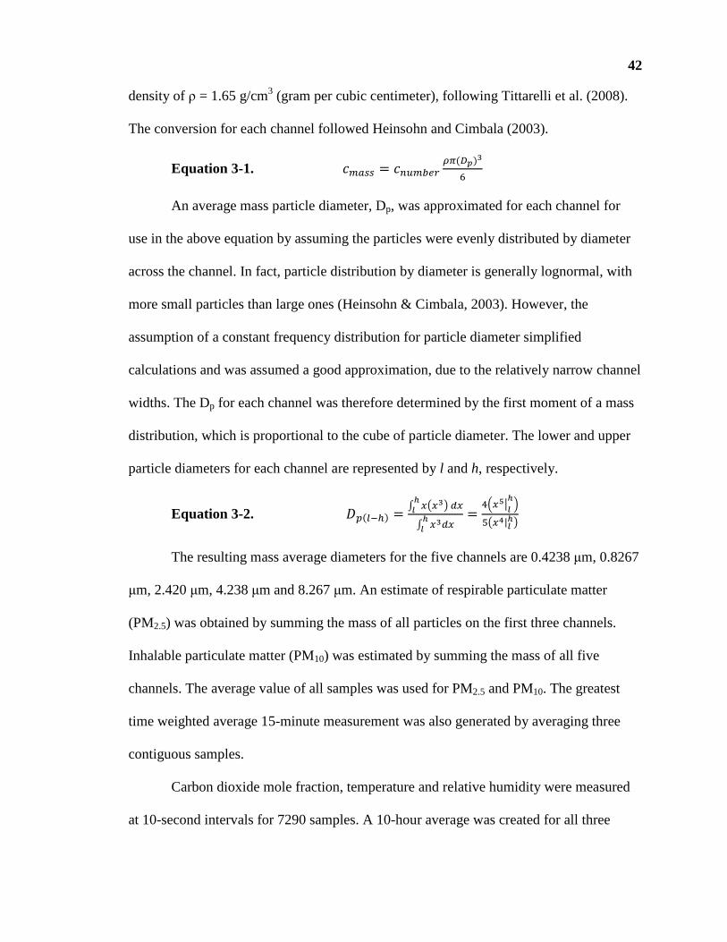
42
density of ρ = 1.65 g/cm3 (gram per cubic centimeter), following Tittarelli et al. (2008).
The conversion for each channel followed Heinsohn and Cimbala (2003).
Equation 3-1. ����� = �������(��)�
�
An average mass particle diameter, Dp, was approximated for each channel for
use in the above equation by assuming the particles were evenly distributed by diameter
across the channel. In fact, particle distribution by diameter is generally lognormal, with
more small particles than large ones (Heinsohn & Cimbala, 2003). However, the
assumption of a constant frequency distribution for particle diameter simplified
calculations and was assumed a good approximation, due to the relatively narrow channel
widths. The Dp for each channel was therefore determined by the first moment of a mass
distribution, which is proportional to the cube of particle diameter. The lower and upper
particle diameters for each channel are represented by l and h, respectively.
Equation 3-2. ��(���) =� ���������� ���� ��
= !"�#$��%
&�"�'|���
The resulting mass average diameters for the five channels are 0.4238 µm, 0.8267
µm, 2.420 µm, 4.238 µm and 8.267 µm. An estimate of respirable particulate matter
(PM2.5) was obtained by summing the mass of all particles on the first three channels.
Inhalable particulate matter (PM10) was estimated by summing the mass of all five
channels. The average value of all samples was used for PM2.5 and PM10. The greatest
time weighted average 15-minute measurement was also generated by averaging three
contiguous samples.
Carbon dioxide mole fraction, temperature and relative humidity were measured
at 10-second intervals for 7290 samples. A 10-hour average was created for all three

43
variables by averaging the samples. In addition, a maximum time weighted average 15-
minute carbon dioxide mole fraction was estimated by averaging 90 contiguous samples.
Sound pressure level was measured in 2,640 30-second intervals across octave
bandwidths. These equivalent levels were A-weighted and combined logarithmically to
create an equivalent sound pressure level over 10 hours. The 1% and 99% sound pressure
levels were also selected from the 30-second sampled data. Reverberation times
calculated from computer software based on 20 dB decay were averaged over the mid
frequencies to create an average time for a direct sound to decay 60 dB.
The fraction of time lights in the classroom were on during the 10-hour period
was estimated using occupied horizontal illuminance measurements taken at 10-second
intervals at the ceiling, facing down. For each classroom, a threshold illuminance was
estimated by investigation of the data, which was assumed to correlate with the lighting
condition. This is possible because lights are turned off predictably during naptime.
A summary of all predictors measured for the study is provided in Table 3-2. All
the predictor data is at the classroom level.

44
Table 3-2: Predictor Variables in the Physical Environment
Variable Description Units General
area Usable floor area of classroom ft2 (square feet)
color Predominant wall color of classroom cool or warm extdoor Presence of a door to the exterior (ext) yes or no
carpet Portion of permanent flooring that is carpet ratio
Acoustic acccontrol Ability to separate room from adjacent spaces yes or no rt20 Reverberation time (rt) based on a decay of 20 dB seconds
bnllow Typical 4-minute (min) minumum unoccupied A-weighted equivalent sound pressure level (background noise level abbreviated bnl)
dB (decibels) re 20µPa (micropascals)
bnlhigh Typical 4-min maximum unoccupied A-weighted equivalent sound pressure level
dB re 20µPa
bnldelta Difference between bnllow and bnllhigh dB
laeq10 A-weighted, equivalent sound pressure level (LAeq) during a 10-hour (hr) occupied period
dB re 20µPa
l1 A-weighted sound pressure level (l) of 1% threshold during a 10-hr occupied period
dB re 20µPa
l99 A-weighted sound pressure level of 99% threshold during a 10-hr occupied period dB re 20µPa
Temperature
temp10 Temperature (temp) averaged over 10 hrs from measurements every 10 seconds (secs)
Fahrenheit degrees
rh10 Relative humidity (rh) averaged over 10 hrs from measurements every 10 secs
ratio
tstat Condition of a thermostat (tstat) in the room ordinal
Lighting
switches Number of controllable lighting zones in the classroom
numeric
orient Azimuth degree angle of exposure of classroom windows (0º is North)
degrees
glarecontrol Portion of windows with protection from insolation ratio lpd Lighting power density (lpd) Watts/ft2 illum Average high illuminance (illum) footcandles
illumratio Ratio between average high and average low illuminance
ratio
onoff10 Percentage of time lights are off during a 10-hr period ratio

45
Table 3-2: Predictor Variables in the Physical Environment, continued
Variable Description Units Air Quality
pm2510 Average mass concentration of respirable particulate matter (pm2.5) averaged over a 10-hr period
µgrams (micrograms) per m3(cubic meter)
pm2515 Maximum 15-min time-weighted average mass concentration of respirable particulate matter over a 10-hr period
µgrams/m3
pm1010 Average mass concentration of inhalable particulate matter (pm10) averaged over a 10-hr period
µgrams/m3
pm1015 Maximum 15-min time-weighted average mass concentration of inhalable particulate matter over a 10-hr period
µgrams/m3
co210 Carbon dioxide (CO2) concentration averaged over a 10-hr period
parts per million (ppm)
co215 Maximum 15-min carbon dioxide concentration over a 10-hour period
ppm
Visual inspection of time-series data plots for each variable provided confirmation
of reliability and instrumentation. Appendix A, Figure A-1 through Figure A-4 contain
plots for two of the 31 rooms measured. Some other notes on data measurements are as
follows. Data collection at room A28 for occupied measures terminated at 17:09 instead
of 17:30 due to study limitations. For comparison with other data, the measures were
extrapolated from the last record from the classroom, which was already unoccupied at
17:09. Data collection for B19 began at 8:00 p.m. instead of 7:30 p.m. on the day prior to
occupied measures, although this did not affect the study variables.
At room A27, PM10 mass concentration spiked at 5:14 p.m. to 782 µg/m3. This
level is a factor of 10 greater than the typical levels and it was not sustained. Therefore,
this data point was thrown out, since it was unlikely the level was caused by regular
activities in the classroom because most children had left the center and cleaning begun.

46
In Room A88, the PM2.5 and PM10 mass concentrations peaked at 187 µg/m3 and
2254 µg/m3, respectively. By investigation, the data suggest these levels of suspension
were obtained from normal activity with a steady change in concentration from about
10:20 a.m. to 11:40 a.m. For this room, three days of continuous data was available for
particulate matter, and, to understand better activity in the room, all three days were
investigated. Plots of these levels in Room A88 are provided in Appendix A, Figure A-5,
Figure A-6 and Figure A-7. At room B33, measures began at 8:00 p.m. and terminated at
5:00 p.m. The CO2 meter appears to have turned off due to power supply at 4:45 p.m.,
and the remaining 15 minutes of measures were extrapolated from the last recording.
Facility age was eliminated as a variable because school was used instead to
represent the same test and was less likely to lead to assumptions from non-
independence. Similarly, the items for acoustics controllability and thermostat were not
used in the analysis because one of the schools had little or no variance on the variable.
SECTION 3.2 - Outcome Variable: Teacher Satisfaction
The self-assessment used was based on the Occupant Indoor Environmental
Quality Survey (Center for the Built Environment, 2004). The researcher developed the
tool presented in Appendix C because a written survey was necessary for broad
participation by teachers and the Occupant Indoor Environmental Quality Survey was
only available as a web-based tool. Items related to satisfaction with the social work
environment were included based on findings in the literature review. The Quantum
Workplace (2015) Best Places to Work survey generated a pool of seven such items.

47
Modifications to the items from both reference surveys included item wording to
increase the item relevance for the target audience. Semantic differential scales were used
for IEQ items, and Likert scales were used for organizational satisfaction items (Dykes &
Baird, 2013). These scales are ordinal which present limitations to statistical inferences.
A 6-point scale was selected for all items. The overall item pool was selected to result in
a questionnaire that takes less than 15 minutes to complete. Items were selected to
facilitate aggregation into composite scores. Items are aggregated often to improve
reliability of assessments (Cohen et al., 2013). Table 3-3 summarizes the survey items.
Participants completed the survey at a staff-training event on March 12, 2015 that
occurred at a facility other than the schools involved in the study. All teachers were
expected to attend this training, and time was allotted for those who wanted to participate.
The target audience was the three teachers in each of the 31 classrooms in the study, for
93 targeted participants. To protect confidentiality, all teachers were provided with a
survey that included the consent form in the front matter. Those who did not want to
participate could still complete the survey with the knowledge that it would be destroyed
if it lacked their signature on the consent form. In total, 87 teachers received surveys, and
70 teachers returned them. Of those returned, 48 teachers consented to participate, and 44
of the consenting teachers were assignable to a classroom included in the study. Teachers
were not paid to participate.
Participants are distributed across classrooms and schools based on age, teaching
experience, teaching position and length of time assigned to the same classroom.
Participant characteristics are described in Table 3-4 and Table 3-5.

48
Table 3-3: Survey Response Items
Variable Name Item
Cla
ssro
om S
ize
sizepersonal How satisfied are you with the amount of space available for your use and storage?
sizechild How satisfied are you with the amount of space available for children?
sizeinterfere Does the classroom size interfere with your ability to do your job?
Cla
ssro
om V
iew
s
viewcoworker How satised are you with the ability to … see your co-workers?
viewprivacy How satisfied are you with the privacy of your classroom from the outdoors and hallway?
viewnature How satisfied are you with the quality of view to … nature?
viewinterfere Do the classroom views interfere with your ability to do your job?
Aco
ustic
s
bnlsat How satisfied are you with the sound level in your classroom? (Background noise level abbreviated bnl.)
stcsat How satisfied are you with the ability to keep noise from other spaces out…? (Sound Transmission Class abbreviated STC.)
claritysat How satisfied are you with the ability for the children to understand you…?
accprob Which of the following create noise problems…? accinterfere Do the acoustics interfere with your ability to do your job?
Tem
pera
ture
tempcontrol Which of the following can you personally control…?
tempsat How satisfied are you with the temperature for your comfort…?
tempchild How satisfied are you with the temperature for children’s comfort…?
tempprob Check all that apply about the temperature…: [inverted scale] tempinterfere Does the temperature interfere with your ability to do your job?
Air
Qua
lity airsat
How satisfied are you with the air quality in your classroom?
airprob Which of the following contribute to odor problems…?
airinterfere Does the air quality interfere with your ability to do your job?

49
Table 3-3: Survey Response Items, continued
Variable Name Item
Ligh
ting
lightcontrol Which of the following can you personally control…? lightsat How satisfied are you with the electric light in your classroom?
lightprob Check all that apply about the electric light…: naturalsat How satisfied are you with the daylight… in your classroom?
naturalprob Check all that apply about the daylight…: lightinterfere Does the lighting interfere with your ability to do your job?
Fur
nitu
re
furnadult How satisfied are you with the comfort of furniture for adults?
furnchild How satisfied are you with the comfort of furniture for children?
furnadjust How satisfied are you with ... the adjustability of furniture? furnlayout How satisfied are you with the furniture layout…?
finishes How satisfied are you with the colors and textures …? furninterfere Does the furniture interfere with your ability to do your job?
Cle
anin
g
cleanorg How satisfied are you with the tidiness of your classroom?
cleanservice How satisfied are you with the cleaning service in your classroom?
cleandisplay How satisfied are you with the wall display surfaces? cleanprob Which of the following are problems…?
cleaninterfere Does the cleaning and organization interfere with your ability to do your job?
Org
. Sat
isfa
ctio
n enjoy I enjoy my work.
team My team works well together. invests My employer invests to make me more successful.
paid I am paid fairly. purpose I understand the purpose of my organization.
quit It would take a lot to get me to leave this job. friends I have a trusting relationship with one or more co-workers.
ieqoverall All things considered, how satisfied are you with your classroom? (Indoor environmental quality abbreviated ieq.)
Eight items on the survey were answered unanimously across all participants and
were therefore removed from the data. All of the participants identified as female. None
of the participants reported conditions that affected their hearing; one reported sinuses

50
that affected her smelling; and several reported corrected vision. One participant reported
an astigmatism that affected her vision. Three teachers provided write-in comments on a
multiple-choice item but did not check the box for the item they listed. One such item
was “Which of the following create noise problems? (Check all that apply),” to which the
participants responded, “Adjoining bathroom, other classroom uses it and is loud during
our nap time” and “Kids on playground outside make noise.” These were coded
respectively as “People in other classrooms” and “Outdoor noise.” A second item was
“Are there other issues with the lighting?,” to which one participant responded, “Want
shades on doors, too bright at nap times.” This was coded as “Sunlight is too bright at
times.” The researcher coded these write-in items as if they had selected the more general
item listed.
Data preparation included collapsing several items into single variables. Items
that listed control features or problem areas were counted, with the number of instances
“checked” reported into a single variable. For example, the item “Which of the following
can you personally control in your classroom (check all that apply)?” was collapsed into a
single item as the number of items checked. In this specific case, “light dimmer” was one
of the choices. However, none of the rooms have dimmer switches for the ambient
lighting; therefore, the two participants who reported this feature were confused,
malingering, or referring to other lighting features in the space. The target construct for
the item is the perception of control of the lighting; thus, the “light dimmer” item was
retained.

51
Table 3-4: Participant Characteristics by Classroom Type
Classroom Type Infant
6 wks-1 yr Toddler 1-2 yrs
Toddler 2-3 yrs
Preschool 3-5 yrs Total
Teaching Experience (years)
<1 0 3 1 0 4 1-3 1 3 3 1 8 3-10 5 3 2 5 15 >10 3 7 4 3 17
Age (years)
<30 4 6 5 3 18 31-40 0 7 4 2 13 41-50 2 2 1 1 6 >50 3 1 0 3 7
Time in Classroom
<3 months 2 0 0 0 2 3-12 months 2 10 3 2 17 1-3 years 3 4 5 2 14 > 3 years 2 2 2 5 11
Title Lead Teacher 2 5 6 5 18 Associate Teacher 4 7 1 3 15 Teacher's Aide 3 4 3 1 11
Total 9 16 10 9 44

52
Table 3-5: Participant Characteristics by School
School A School B Total Participants 21 23 44
Classrooms
1 Survey 3 4 7 2 Surveys 6 5 11 3 Surveys 2 3 5 Total 11 12 23
Teaching Experience (years)
<1 3 1 4 1-3 4 4 8 3-10 10 5 15 >10 4 13 17
Age (years)
<30 13 5 18 31-40 3 10 13 41-50 2 4 6 >50 3 4 7
Time in Classroom
<3 months 2 0 2 3-12 months 7 10 17 1-3 years 6 8 14 > 3 years 6 5 11
Title Lead Teacher 9 9 18 Associate Teacher 7 8 15 Teacher's Aide 5 6 11
SECTION 3.3 - The Predictive Model
The study hypothesizes that measures of the physical environment can predict
teacher satisfaction with IEQ. The proposed model links a specific variable in the
physical environment to an outcome measure from the teacher survey. Survey items were
grouped into domain composites to improve reliability. As illustrated in the literature
review, domains are interrelated; therefore, a secondary hypothesis is that variables from

53
the physical environment in one domain can predict teacher satisfaction in a different
domain. Teacher characteristics and organizational satisfaction are hypothesized to
mediate these relationships between the physical environment and perception of IEQ.
Finally, the physical environment is hypothesized to predict global perception of IEQ.
Two IEQ composite scores were evaluated – one that targeted variables most related to
human physiology and another that included broader measures, such as furniture and
cleanliness.
The hypotheses of this study are at the classroom level as the unit of treatment of
the physical environment. However, the theory guiding the research design emphasizes
the role of individual differences on behavioral responses to the physical environment.
Multilevel modeling with random intercepts at the school and classroom levels provides a
concise method for inferential tests of the nested data. However, the limited sample of
teachers at both school and classroom levels rendered this approach untenable. For
classrooms with more than one participant, one approach would be to average the surveys
together, aggregating individual data at the classroom level for analysis. While this could
improve reliability, it also makes individual differences such as age, gender, experience
and organizational satisfaction less meaningful. Therefore, the study instead selected a
representative teacher from each classroom for data analysis. This allowed a multivariate
linear regression model comparison approach to data analysis.
Teachers are grouped also by school; therefore, survey responses will likely
exhibit nonindependence at the school level. To accommodate this structure, school was
included as a categorical predictor in both compact and augmented models. This means
each finding must be interpreted with respect to the effect of school. Where school did

54
not explain a moderate level of variance in teacher scores, it was omitted to improve
statistical power.
For the results listed in Chapter 4, the following steps were consistent across each
domain. Teacher responses to each survey item in a domain were converted to z scores. If
items counted the number of problems, the score was inverted so that the effect directions
were similar. Survey items then were selected to form a composite based on Cronbach’s
alpha values and inspection of Pearson’s correlation tables. Cronbach’s alpha is a
common measure of item agreement that is used often to support the internal reliability of
a set of items. It is similar to an average of item correlation coefficients where the
number of items proportionally increases alpha. A high value of alpha, e.g. 0.7 or 0.8, is
not necessarily an indication that the items measure a one-dimensional construct. One
risk in eliminating items to increase Cronbach’s alpha is that the construct validity of the
assessment may suffer (Cho & Kim, 2015). Therefore, composites for this study are
formed based on judgment with consideration for the resulting alpha.
The newly formed composite score was evaluated for variance explained by
school, classroom type, teacher age, teacher experience, teacher organizational
satisfaction and the length of time the teacher has been assigned to the classroom. In
general, only the variable school explained considerable variance and was retained in the
compact model. Finally, each measurement in the physical environment was added to the
model to evaluate its predictive power in a 1-degree of freedom test. The software
package R was used for all statistical calculations and for preparation of figures (R Core
Team, 2012). An example model comparison follows.
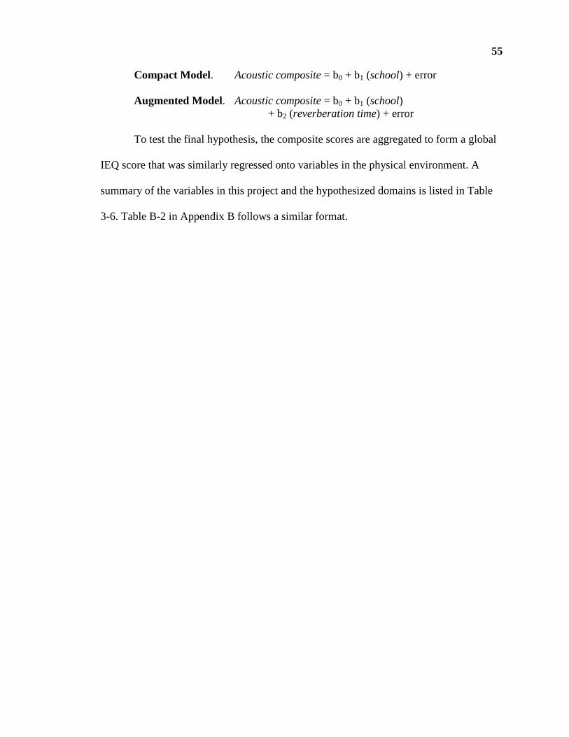
55
Compact Model. Acoustic composite = b0 + b1 (school) + error Augmented Model. Acoustic composite = b0 + b1 (school) + b2 (reverberation time) + error
To test the final hypothesis, the composite scores are aggregated to form a global
IEQ score that was similarly regressed onto variables in the physical environment. A
summary of the variables in this project and the hypothesized domains is listed in Table
3-6. Table B-2 in Appendix B follows a similar format.

56
Table 3-6: Study Hypotheses
Domain Response Variable Predictor Variable Mediator Size sizepersonal,
sizechild, sizeinterfere
area school, crtype orgsat, tenure, teachage
Views viewcoworker, viewprivacy, viewnature, viewinterfere
area, color, blindsopen, glarecontrol
school, crtype orgsat, tenure, teachage
Acoustics accoverall, bnlsat, stcsat, claritysat, accprob
acccontrol, rt20, bnllow, bnlhigh, laeq10, l1, l99
school, crtype orgsat, tenure, teachage
Lighting lightoverall, lightcontrol, lightsat, lightprob, naturalsat, naturalprob
illum, illumratio, lpd, glarecontrol blindsopen, onoff10, orient
school, crtype orgsat, tenure, teachage
Temperature thermcontrol, thermsat, thermprob, thermoverall
tstat, temp10, rh10
school, crtype orgsat, tenure, teachage
Air Quality airsat, airprob, airoverall
pm2510, pm1515, pm1010, pm1015, co210, co215
school, crtype orgsat, tenure, teachage
Furnishings furnadult, furnchild, furnadjust, furnlayout, finishes, furninterefere
area, color, carpet, plants, hiding
school, crtype orgsat, tenure, teachage
Cleaning cleanorg, cleanservice, cleandisplay,cleanprob, cleaninterfere
carpet, plants school, crtype orgsat, tenure, teachage
Overall IEQ ieqoverall all measures in the physical environment
school, crtype orgsat, tenure, teachage

57
CHAPTER 4 - Results
SECTION 4.1 - Survey Findings
The preliminary dataset for analysis was formed from responses on 45 survey
items by 44 participants. Teachers in the same room answered similarly on the 38 survey
items related to IEQ, although inter-rater reliability was low. In rooms with 2 or 3
teachers, the intraclass correlation coefficient (two-way, consistency type) ranged from
0.31 to 0.83, with an average of 0.56. Figure 4-1 shows how two teachers in the same
classroom responded on items using the scale of 1 (dissatisfied) to 6 (satisfied).
Classroom A18 demonstrated good agreement, with an intraclass correlation of 0.83,
while classroom B97 had a poor intraclass correlation of 0.31.
Figure 4-1: Classrooms A18 & B97 Teacher Agreement
Figure 4-2 illustrates the agreement between scores in classrooms with three
teachers. Classroom A19 demonstrated good agreement with an intraclass correlation of
0.77, while classroom B12 demonstrated poor agreement with an intraclass correlation of
0.41. The histogram of responses from two teachers in Room B89 presented in Figure
4-3 illustrates the low reliability of raters.
0 1 2 3 4 5 6
01
23
45
6
A18 Teacher 1
A1
8 T
each
er 2
0 1 2 3 4 5 6
01
23
45
6
B97 Teacher 1
B9
7 T
each
er 2

58
Figure 4-2: Classrooms A19 & B12 Teacher Agreement
Figure 4-3: Classroom B89 Teacher Response Histograms
Analysis proceeded with the creation of three datasets with 23 participants each,
seeded from the full dataset of 44 participants. Where multiple teacher scores were
available for a classroom, individuals were selected based on job title. The first dataset
(survdat1 ) was composed of Lead Teachers to the greatest extent possible and contained
5 Associate Teachers. The second dataset (survdat2) contained mostly Associate
Teachers with 8 Lead Teachers. The third dataset (survdat3) included Teacher’s Aides
to the greatest extent possible, with the second choice being Lead Teacher. This dataset
contained 11 Teacher’s Aides, 10 Lead Teachers and 2 Associate Teachers. Figure B-1,
A19-1A19-2
A19-3
B12-1B12-2
B12-3
Teacher 1
Fre
qu
ency
0 1 2 3 4 5 6
02
46
81
2
Teacher 2
Fre
qu
ency
0 1 2 3 4 5 6
05
10
15
20
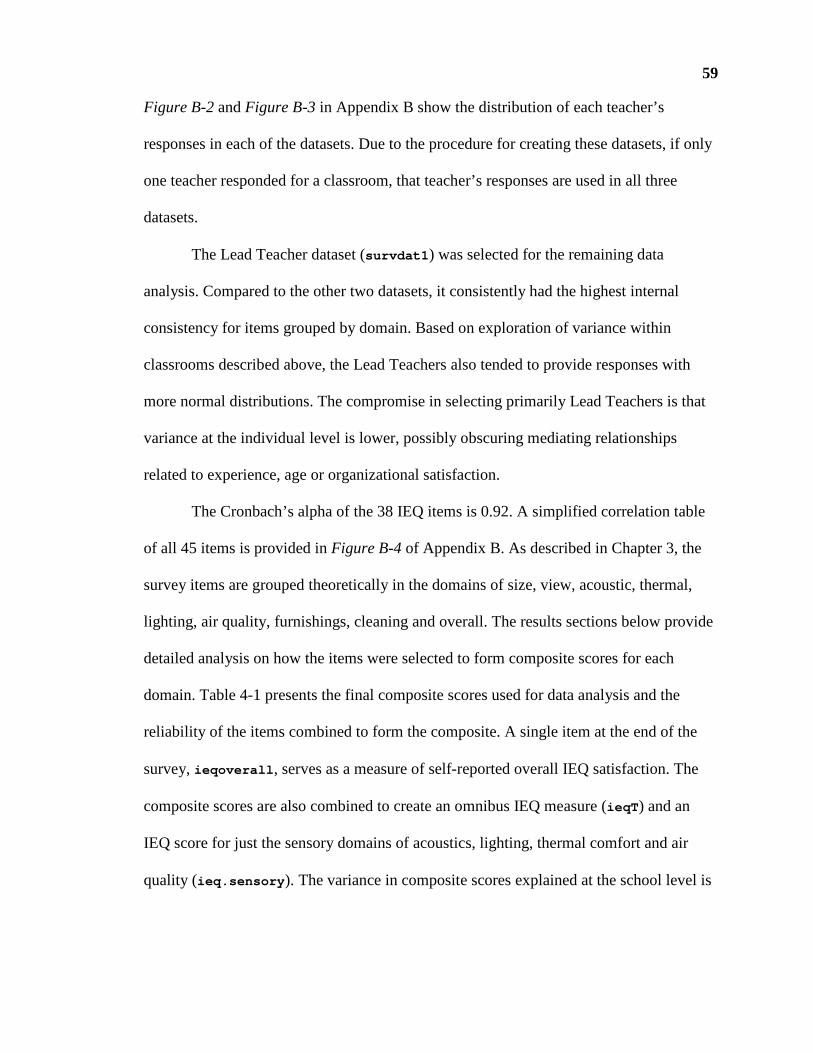
59
Figure B-2 and Figure B-3 in Appendix B show the distribution of each teacher’s
responses in each of the datasets. Due to the procedure for creating these datasets, if only
one teacher responded for a classroom, that teacher’s responses are used in all three
datasets.
The Lead Teacher dataset (survdat1 ) was selected for the remaining data
analysis. Compared to the other two datasets, it consistently had the highest internal
consistency for items grouped by domain. Based on exploration of variance within
classrooms described above, the Lead Teachers also tended to provide responses with
more normal distributions. The compromise in selecting primarily Lead Teachers is that
variance at the individual level is lower, possibly obscuring mediating relationships
related to experience, age or organizational satisfaction.
The Cronbach’s alpha of the 38 IEQ items is 0.92. A simplified correlation table
of all 45 items is provided in Figure B-4 of Appendix B. As described in Chapter 3, the
survey items are grouped theoretically in the domains of size, view, acoustic, thermal,
lighting, air quality, furnishings, cleaning and overall. The results sections below provide
detailed analysis on how the items were selected to form composite scores for each
domain. Table 4-1 presents the final composite scores used for data analysis and the
reliability of the items combined to form the composite. A single item at the end of the
survey, ieqoverall , serves as a measure of self-reported overall IEQ satisfaction. The
composite scores are also combined to create an omnibus IEQ measure (ieqT ) and an
IEQ score for just the sensory domains of acoustics, lighting, thermal comfort and air
quality (ieq.sensory ). The variance in composite scores explained at the school level is

60
included in Table 4-1 for interpretation of results and to describe the variance that
remains to be explained by predictors in the physical environment.
Because scaled and centered scores are used throughout the analysis, Table B-1 in
Appendix B presents raw scores for each composite to provide an understanding of
absolute differences in teacher responses. Both Table 4-1 and Table B-1 show differences
between schools in teacher satisfaction with classroom size, acoustics, natural light,
furniture and cleaning.
Several of the composite scores shown in Table 4-1 are correlated. Table 4-2
provides the Pearson’s correlations. Because all composites are self-reported perceptions
of IEQ, these relationships are less valuable for understanding relationship in the physical
environment than they are for investigating latent factors in the perception of IEQ.
Some of the significant correlations in the sensory domains are plotted in Figure
4-4 to illustrate the level of agreement between items for teachers and to qualify the
statistical tests for the small and convenient sample. As suggested by the literature, there
is a correlation between the perception of thermal comfort and air quality. However, the
other correlations, such as that between air quality and acoustics, were not anticipated.
Also of note is that satisfaction in the sensory domains does not predict overall
satisfaction. A common correlation with overall IEQ would help explain the inter-sensory
correlations that are otherwise challenging to interpret.

61
Table 4-1: Composite Scores and Constituent Items
Composite (# of items)
Survey Items Cronbach’s Alpha (α)
Variance Attributable to School
sizesat (2) sizepersonal , sizechild, sizeinterfere 0.83 18%*
viewsat (3) viewcoworker, viewprivacy, viewnature, viewinterfere 0.74 11%
accsat2 (3) bnlsat, stcsat, claritysat, accprob , accinterfere 0.66 17%*
thermsat (4) tempcontrol , tempsat, tempchild, tempprob, tempinterfere 0.84 2%
airtot (3) airsat, airprob, airinterfere 0.73 0%
lighttot (2) lightcontrol , lightsat, lightprob 0.19 5%
naturaltot (2) naturalsat, naturalprob, lightinterfere 0.53 19%*
furntot (6) furnadult, furnchild, furnadjust, furnlayout, finishes, furninterefere
0.87 21%*
cleantot (5) cleanorg, cleanservice, cleandisplay,cleanprob, cleaninterfere
0.85 29%*
orgsat (7) enjoy, team, invests, paid, purpose, quit, friends 0.80 1%
ieqoverall (1) ieqoverall N/A 0%
ieq.sensory (5) accsat2, thermsat, airtot, lighttot, naturaltot 0.67 4%
ieqT (9) sizesat, viewsat, accsat2, thermsat, airtot, lighttot, naturaltot, furntot, cleantot
0.84 16%
* significant at the p < 0.05 level

62
Table 4-2: Composite Score Pearson’s Correlations
Composite 1 2 3 4 5 6 7 8 9 10
1 sizesat -
2 viewsat 0.54 **
-
3 accsat2 0.50
* 0.58 **
-
4 thermsat 0.22 0.28 0.51
* -
5 airtot 0.09 0.37 0.53
* 0.44
* -
6 lighttot -0.01 0.29 0.30 0.31 0.47
* -
7 naturaltot 0.59 **
0.55 **
0.33 -0.01 -0.04 0.08 -
8 furntot 0.47
* 0.65 ***
0.61 **
0.38 0.43
* 0.25 0.35 -
9 cleantot 0.66 ***
0.60 **
0.45 *
0.16 0.28 0.02 0.47
* 0.74 ***
-
10 orgsat 0.35 0.32 0.13 -0.32 -0.12 0.24 0.42
* 0.20 0.30 -
11 ieqoverall 0.53 **
0.52 *
0.22 0.07 0.20 0.26 0.26 0.18 0.49
* 0.38
* p < 0.05 ** p < 0.01 *** p < 0.001

63
Figure 4-4: Sensory Composite Score Agreement
To explore further the composite interrelationships, Table 4-3 is presented in a
graphical format that includes the number of significant correlations. For this purpose, the
significance level is p < 0.1. As expected, the two overall IEQ composite items show the
greatest number of relationships to other composite scores. In addition, satisfaction with
classroom size, views and furnishings are related strongly to the other composites.
-2.0 -1.0 0.0 1.0
-2.0
-1.0
0.0
0.5
1.0
Air Composite Score
Ele
ctric
Lig
ht C
om
posi
te S
core
-2.0 -1.0 0.0 1.0
-2-1
01
Air Composite Score
Aco
ustic
Com
posi
te S
core
-2.0 -1.0 0.0 1.0
-10
12
Air Composite Score
Th
erm
al C
ompo
site
Sco
re
-1 0 1 2
-2-1
01
Thermal Composite Score
Aco
ustic
Com
posi
te S
core

64
Satisfaction with electric lighting and organizational satisfaction share the fewest
relationships with the other composite items.
Table 4-3: Composite Score Spearman’s Correlations
Composite Score 1 2 3 4 5 6 7 8 9 10 11 12 13 Count
1 sizesat 9
2 viewsat 8
3 accsat2 7
4 thermsat 6
5 airtot 5
6 lighttot 3
7 naturaltot 7
8 furntot 8
9 cleantot 7
10 orgsat 4
11 ieqoverall 7
12 ieq.sensory 10
13 ieqT 11
p < 0.001 p < 0.01 p < 0.1
SECTION 4.2 - Organizational Satisfaction Results
Seven survey items measure organizational satisfaction. Although they appear at
the end of the survey, the results are provided before the IEQ items because
organizational satisfaction is hypothesized to mediate relationships with IEQ. The items
are reliable with a Cronbach’s alpha of 0.80, and all are retained to form the composite
score orgsat for use in analysis. A summary of the items and correlation is provided in
Table 4-4.

65
Table 4-4: Pearson’s Correlations of Organizational Satisfaction Items
Survey Item Summary Variable 1 2 3 4 5 6
I enjoy my work. 1 enjoy -
My team works well together. 2 team 0.33 -
My employer invests to make me more successful.
3 invests 0.54 **
0.11 -
I am paid fairly. 4 paid 0.38 0.05 0.52
* -
I understand the purpose of my organization.
5 purpose 0.51
* 0.32 0.31 0.46 -
It would take a lot to get me to leave this job.
6 quit 0.45
* 0.30
0.56 **
0.30 0.40 -
I have a trusting relationship with one or more co-workers.
7 friends 0.52
* 0.52
* 0.48
* 0.10
0.45 *
0.47
Organizational satisfaction is correlated with satisfaction with natural light as
shown in Table 4-2. It is a moderate predictor of the overall IEQ item. As discussed in
more detail below, orgsat moderates other relationships between the physical
environment and satisfaction, although no features of the physical environment predict
organizational satisfaction. Other individual level characteristics, such as age and length
of time assigned to same classroom, did not significantly mediate relationships between
composite scores and the physical environment.
SECTION 4.3 - Room Size Results
4.3.1- Survey results. Three items on the survey targeted satisfaction with room
size. These were size personal , sizechild and sizeinterfere . The latter two items
were well correlated with a Cronbach’s alpha of 0.83 and combined to form the
composite score sizesat . The items and correlations are provided in Table 4-5.
Satisfaction with room size varies between schools, as shown in the distribution of scores

66
in Figure 4-5 and the means provided in Appendix B, Table B-1. Teachers at School A
were more satisfied with their room size by 1.0 points on the 6-point scale.
Table 4-5: Pearson’s Correlations of Size Items
Survey Item Summary Variable 1 2 3
How satisfied are you with the amount of space available for your use and storage?
1 sizepersonal -
How satisfied are you with the amount of space available for children?
2 sizechild 0.53 ***
-
Does the classroom size interfere with your ability to do your job?
3 sizeinterfere 0.39 0.73 ***
-
4.3.2- Measurement results. Floor area is the only variable in the study that is
hypothesized to impact teachers’ satisfaction with classroom size. The average area is
about 711 square feet at both schools, as shown in Table A-1, although the deviation at
School A is 3 times larger than the deviation at School B. This relationship is illustrated
in Figure 4-5.
Figure 4-5: Size Composite Score and Area by School
A B
-2.0
-1.0
0.0
1.0
School
Siz
e C
om
po
site
Sco
re
A B
55
06
50
75
08
50
School
Are
a (s
qu
are
feet
)

67
4.3.3- Findings. Data analysis shows that floor area is a good predictor of
satisfaction with classroom size. The statistical tests with significant results are listed in
Table B-2. When the size composite score was regressed onto school, area and
interaction schoolXarea, both school (p = 0.029) and the interaction term (p = 0.053)
were moderate predictors, while area was not (p = 0.914). The analysis also shows area
is significantly more predictive of teacher satisfaction at School B than at School A, as
well as in classrooms with younger children. When the interaction term is omitted from
the model, area is a significant predictor (p = 0.000) along with school (p = 0.004). One
interpretation of the data is that teachers at School B are dissatisfied with small
classrooms for infants (Classroom Type 0). The overall relationship between area and
satisfaction as well as the school interaction is illustrated in Figure 4-6.
Figure 4-6: Area and Size Composite Score Overall and by School
Figure 4-7 shows the interaction of area and the size composite score across
classrom types. When the size composite score is regressed onto classroom type
(crtype ), area and interaction area Xcrtype , area is a good predictor with classroom
Floor Area (square feet)
Siz
e C
ompo
site
Sco
re
-2
-1
0
1
600 700 800 900
School A & B
600 700 800 900
School A
600 700 800 900
School B

68
type and the interaction, both being moderate predictors. This may be explained by the
fact that older children at School B have larger classrooms.
When the size composite score is regressed onto unoccupied background noise
level (bnllow ) and school , bnllow is significant (p = 0.018), with each A-weighted
sound pressure level (dB) increase lowering satisfaction levels by 0.17 standard
deviations. When the composite score sizesat is regressed onto bnllow, school and
the interaction term bnllow Xschool , the interaction is a moderate predictor (p = .068),
and bnllow is not significant. These relationships are plotted in Figure 4-8. When the
size composite score is regressed onto bnllow , classroom type (crtype ) and the
interaction bnllow Xcrtype , bnllow is significant (p = 0.004), and crtype and the
interaction are both moderate predictors (p < 0.10). This relationship is shown in Figure
4-9, and all regression tests are listed in Table B-2 of Appendix B. This finding suggests
that teachers may be more sensitive to background noise in classrooms with younger
children. Reverberation time is also a moderate predictor of size satisfaction scores,
although reverberation time is strongly correlated with area, which is hypothesized as a
confound that explains this result. Classroom type did not predict the size composite
score.

69
Figure 4-7: Area and Size Composite Score by Classroom Type
School
Siz
e C
om
posi
te S
core
-2
-1
0
1
A B
Infant
A B
Toddler 1
A B
Toddler 2
A B
Pre-K
School
Flo
or
Are
a (
squa
re f
ee
t)
600
700
800
900
A B
Infant
A B
Toddler 1
A B
Toddler 2
A B
Pre-K
Floor Area (square feet)
Siz
e C
om
posi
te S
core
-2
-1
0
1
600 700 800 900
Infant
600 700 800 900
Toddler 1
600 700 800 900
Toddler 2
600 700 800 900
Pre-K

70
Figure 4-8: Size Composite Score by BNL
Figure 4-9: Size Composite Score by BNL and Classroom Type
SECTION 4.4 - View Results
4.4.1- Survey results. Four items on the survey asked teachers to report
satisfaction with views related to their classroom space. Three items were selected to
increase Cronbach’s alpha from 0.70 to 0.74, creating the composite score viewsat . The
items used are viewcoworker , viewprivacy and viewnature . The view composite score
is not different between schools, with larger variance at School B, as indicated in Figure
4-10.
Unoccupied Quiet BNL (dBA re. 20µPa)
Siz
e C
om
posi
te S
core
-2
-1
0
1
30 35 40 45
School A
30 35 40 45
School B
30 35 40 45
School A & B
Unoccupied Quiet BNL (dBA re. 20µPa)
Siz
e C
om
posi
te S
core
-2
-1
0
1
30 35 40 45
Infant
30 35 40 45
Toddler 1
30 35 40 45
Toddler 2
30 35 40 45
Pre-K
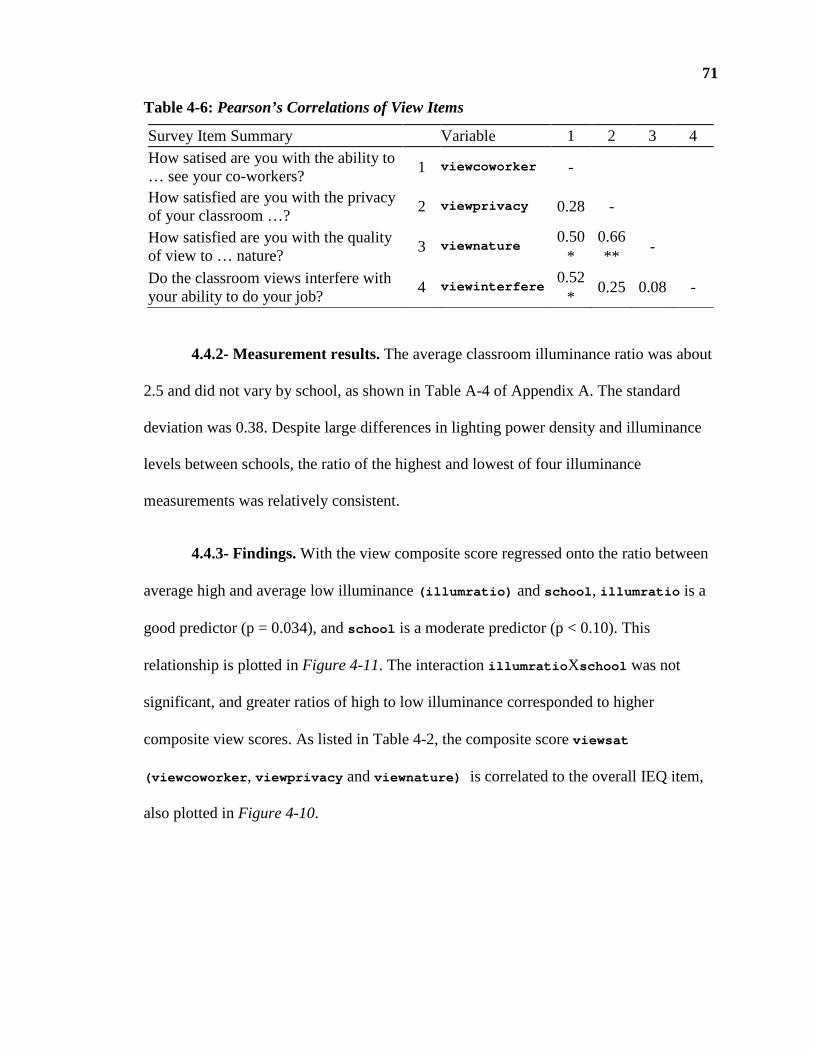
71
Table 4-6: Pearson’s Correlations of View Items
Survey Item Summary Variable 1 2 3 4 How satised are you with the ability to … see your co-workers?
1 viewcoworker -
How satisfied are you with the privacy of your classroom …?
2 viewprivacy 0.28 -
How satisfied are you with the quality of view to … nature?
3 viewnature 0.50
* 0.66 **
-
Do the classroom views interfere with your ability to do your job?
4 viewinterfere 0.52
* 0.25 0.08 -
4.4.2- Measurement results. The average classroom illuminance ratio was about
2.5 and did not vary by school, as shown in Table A-4 of Appendix A. The standard
deviation was 0.38. Despite large differences in lighting power density and illuminance
levels between schools, the ratio of the highest and lowest of four illuminance
measurements was relatively consistent.
4.4.3- Findings. With the view composite score regressed onto the ratio between
average high and average low illuminance (illumratio) and school , illumratio is a
good predictor (p = 0.034), and school is a moderate predictor (p < 0.10). This
relationship is plotted in Figure 4-11. The interaction illumratio Xschool was not
significant, and greater ratios of high to low illuminance corresponded to higher
composite view scores. As listed in Table 4-2, the composite score viewsat
(viewcoworker , viewprivacy and viewnature) is correlated to the overall IEQ item,
also plotted in Figure 4-10.

72
Figure 4-10: View Composite Score by School and Item ieqoverall
Figure 4-11: View Composite Score by Illuminance Ratio
SECTION 4.5 - Acoustic Results
4.5.1- Survey results. Five items are coded on the survey in the acoustic domain
as described in Table 3-3. Score correlations are presented in Table 4-7. The first three
items (bnlsat , stcsat and claritysat) create the composite acoustic score (accsat2 )
that, together, have a Cronbach’s alpha of 0.66. A broad composite with all five items
also was tested with similar findings, generally having lower significance. Following
these preliminary tests, the three-item composite was used for model comparisons.
Teachers at School A had significantly higher acoustic composite scores than those at
School B, as shown in Figure 4-12 and Table A-3 of Appendix B.
A B
-2-1
01
School
Vie
w C
om
po
site
Sco
re
-1.5 -0.5 0.5 1.5
-2-1
01
Item ieqoverall
Vie
w C
om
po
site
Sco
re
Illuminance Ratio
Vie
w C
ompo
site
Sco
re
-2
-1
0
1
2.0 2.5 3.0
School A
2.0 2.5 3.0
School B

73
Table 4-7: Pearson’s Correlations of Acoustic Outcome Variables
Survey Item Summary Variable 1 2 3 4 5 How satisfied are you with the sound level in your classroom?
1 bnlsat -
How satisfied are you with the ability to keep noise from other spaces out…?
2 stcsat 0.69 ***
-
How satisfied are you with the ability for the children to understand you…?
3 claritysat 0.39 0.10 -
Which of the following create noise problems…? [inverted scale]
4 accprob 0.51
* 0.43
* 0.20 -
Do the acoustics interfere with your ability to do your job?
5 acc-interfere
0.58 **
0.16 0.21 0.44
* -
Figure 4-12: Composite Acoustic Score by School and Classroom Type
4.5.2- Measurement results. Table A-3 in Appendix A summarizes the
acoustical measurements in classrooms. The average reverberation time was 0.43 seconds
and exhibited low variance across rooms. The unoccupied A-weighted background noise
levels are higher than design recommendations at 38 dB re 20µPa when the mechanical
systems were off and 48 dB re 20µPa with heat pumps in heating mode. The average 10-
hour occupied A-weighted equivalent sound pressure level was 66 dB re 20µPa, with a
1% exceedance of 76 dB re 20µPa. These levels are acceptable based on safety
guidelines.
A B
-2-1
01
School
Aco
ust
ic C
om
po
site
Sco
re
0 1 2 3
-2-1
01
Classroom Type
Aco
ust
ic C
om
po
site
Sco
re

74
The schools differed significantly in every measure except reverberation time and
the loud unoccupied background noise level, bnlhigh . Figure 4-13 shows the data
distributions for sound pressure levels. School A is quieter than school B as measured by
1% (l1 ) and 99% (l99 ) exceedance levels, as well as A-weighted, equivalent 10-hour
occupied sound pressure level (laeq10 ). Classroom type did not correspond to scores,
although rooms with older children had higher occupied sound pressure levels. One
notable difference between schools is that, with one exception, all classrooms at School B
are conjoined with an adjacent room without acoustic separation. At School A, rooms are
used frequently as paired units, although teachers can separate the rooms using double-
leaf Dutch doors. There is no significant difference between the schools when the
mechanical system is presumably running, as measured by bnlhigh . On average,
difference between high and low unoccupied background noise levels is a significant 5.6
dB higher at School A than School B.

75
Figure 4-13: Acoustical Measurements Distribution
A B
727
47
678
80
School
1% E
xce
eda
nce
(dB
A r
e.
20µ
Pa)
A B
3540
4550
School
99%
Exc
eeda
nce
(dB
A r
e. 2
0µ
Pa)
A B
303
540
45
School
Qu
iet
Un
occu
pied
BN
L (
dBA
re.
20µ
Pa)
A B
4045
5055
School
Lou
d U
noc
cupi
ed B
NL
(dB
A r
e.
20µ
Pa)
A B
6062
6466
6870
School
Occ
upie
d B
NL
(d
BA
re
. 20
µP
a)
0 1 2 3
6062
6466
6870
Classroom Type
Occ
upie
d B
NL
(d
BA
re
. 20
µP
a)

76
4.5.3- Findings. Reverberation time was significantly related to area (p = 0.008),
a relationship illustrated in Figure 4-14. This presents an inherent confound in the
predictor variables that limits inferences from results involving these variables. With this
in mind, when the composite acoustic score (accsat2) was regressed onto floor area and
school, floor area was a significant predictor (p = 0.015), with school also reaching
significance. When the composite score was regressed onto reverberation time and
school, reverberation time is a moderate predictor (p = 0.092), and school is a good
predictor.
Figure 4-14: Floor Area by Reverberation Time
When the acoustic composite score (accsat2 ) was regressed onto unoccupied
background noise level and school, bnllow reached moderate significance (p < 0.10).
This was also the case for bnlhigh. When the composite score was regressed onto
relative humidity and school, relative humidity is a significant predictor (p = 0.014), with
school being a moderate predictor (p < 0.10). Higher moisture correlated with higher
acoustic composite scores. Relative humidity was also significant when included with
0.38 0.42 0.46 0.50
55
06
50
75
08
50
Reverberation Time (seconds)
Flo
or
Are
a (s
qu
are
feet
)

77
classroom type as a regressor of composite score. Relative humidity was also a moderate
predictor of the five-item composite acoustic score (accsat1 ) in a model with school
included as a regressor. The consistency of this finding suggests that the domains of
thermal comfort and acoustical satisfaction may be interrelated in occupant perception of
IEQ. This is supported further by the correlation of the thermal comfort composite score
with the acoustic composite score, as described in Figure 4-4 and Table 4-2.
Figure 4-15: Acoustic Composite Score by Quiet Unoccupied BNL
Figure 4-16: Acoustic Composite Score by Relative Humidity
Quiet Unoccupied BNL (dBA re. 20µPa)
Aco
ustic
Com
pos
ite S
core
-2
-1
0
1
30 35 40 45
School A
30 35 40 45
School B
Relative Humidity (%)
Aco
ustic
Com
posi
te S
core
-2
-1
0
1
15 20 25
School A
15 20 25
School B
15 20 25
School A & B

78
Occupied sound pressure level did not predict the composite acoustic score,
although it did predict the item stcsat (satisfaction with the ability to keep out noise
from other spaces) as a regressor with school (p = 0.014). This relationship is suggestive
at School A, as illustrated in Figure 4-17. When stcsat was regressed onto laeq10 ( A-
weighted, equivalent 10-hour occupied sound pressure level), school and
laeq10 Xschool , the interaction of school and sound pressure level was not significant.
Figure 4-17: Item stcsat by Occupied BNL Within School
SECTION 4.6 - Temperature Results
4.6.1- Survey results. The five items targeting occupant thermal comfort
combined into the thermsat composite (tempsat , tempchild , tempprob and
tempinterfere) , with the exclusion of tempcontrol . The four items exhibit internal
reliability with a Cronbach’s alpha of 0.84, an increase from the value of 0.76 for all five
items. The item correlations are presented in Table 4-8.
The composite score does not vary by school but does vary by crtype,
classroom type, (p=0.034), as shown in Figure 4-18. When thermal composite scores
Occupied BNL (dBA re. 20µPa)
Ite
m s
tcsa
t
-2
-1
0
1
60 62 64 66 68 70 72
School A
60 62 64 66 68 70 72
School B

79
were regressed onto classroom type and school, classroom type remained a significant
predictor. When thermal composite scores were regressed onto classroom type, school
and the interaction crtype Xschool , the interaction was not significant. This may be due
to a relatively strong trend in School B of greater thermal satisfaction reported in
classrooms with older children. This is represented in Figure 4-19.
Table 4-8: Pearson’s Correlations of Thermal Outcome Variables
Survey Item Summary Variable 1 2 3 4 5 Which of the following can you personally control…?
1 tempcontrol -
How satisfied are you with the temperature for your comfort…?
2 tempsat 0.02 -
How satisfied are you with the temp. for children’s comfort…?
3 tempchild 0.08 0.53 ***
-
Check all that apply about the temperature…: [inverted scale]
4 tempprob -0.10 0.62 **
0.60 **
-
Does the temperature interfere with your ability to do your job?
5 tempinterfere 0.00 0.54 **
0.50 *
0.50 *
-
Figure 4-18: Thermal Composite Score by School and Classroom Type
4.6.2- Measurement results. Temperature and relative humidity were relatively
consistent across classrooms at both schools. Table A-2 in Appendix A includes thermal
comfort measurements at each classroom and shows that temperature at School B was
A B
-10
12
School
Th
erm
al C
om
po
site
Sco
re
0 1 2 3
-10
12
Classroom Type
Th
erm
al C
om
po
site
Sco
re

80
more variable than at School A. This may be related in the distribution of thermal
composite scores between schools shown in Figure 4-18 although, as noted above, there
was not a significant difference in the score means between the schools.
4.6.3- Findings. Average occupied temperature did not predict the thermal
composite score, nor did relative humidity, particulate matter or carbon dioxide
concentration. While the data for predictors and outcomes both exhibit large variance,
there is little difference in the means, and this may explain the lack of a result. Of note is
the correspondence of temperature variance with thermal score variance.
Figure 4-19: Thermal Composite Scores by Classroom Type Within School
Figure 4-20: Temperature by Classroom Type Within School
Classroom Type
The
rma
l Com
posi
te S
core
-1
0
1
2
0 1 2 3
School A
0 1 2 3
School B
Classroom Type
Te
mp
era
ture
(F
°)
70
72
74
76
78
80
0 1 2 3
School A
0 1 2 3
School B

81
Figure 4-21: Thermal Composite Score by Color and Orientation
When thermal composite scores are regressed onto wall color and classroom type,
wall color is a moderate predictor (p = 0.066). As illustrated in Figure 4-21, cool wall
color is associated with higher scores. Thermal scores also varied by classroom
orientation. When the composite score was regressed onto orientation and classroom
type, the orientation was significant (p = 0.039). When the score was instead regressed
onto orientation and school, the orientation was a moderate predictor (p = 0.052).
Teachers in rooms that face southward reported higher thermal composite scores than
those in rooms facing other directions. Figure 4-21 illustrates the relationship by
classroom type. These findings are summarized in Appendix B, Table B-2.
Color (1 = Warm Color)
The
rma
l Com
posi
te S
core
-1
0
1
2
-1 1
Infant
-1 1
Toddler 1
-1 1
Toddler 2
-1 1
Pre-K
Orientation (1 = South-facing)
The
rma
l Com
posi
te S
core
-1
0
1
2
-1 1
Infant
-1 1
Toddler 1
-1 1
Toddler 2
-1 1
Pre-K
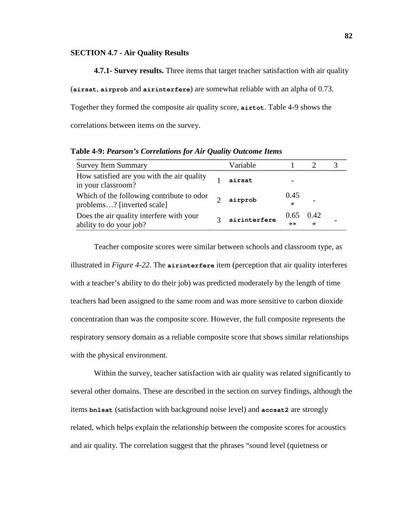
82
SECTION 4.7 - Air Quality Results
4.7.1- Survey results. Three items that target teacher satisfaction with air quality
(airsat , airprob and airinterfere ) are somewhat reliable with an alpha of 0.73.
Together they formed the composite air quality score, airtot . Table 4-9 shows the
correlations between items on the survey.
Table 4-9: Pearson’s Correlations for Air Quality Outcome Items
Survey Item Summary Variable 1 2 3 How satisfied are you with the air quality in your classroom?
1 airsat -
Which of the following contribute to odor problems…? [inverted scale]
2 airprob 0.45
* -
Does the air quality interfere with your ability to do your job?
3 airinterfere 0.65 **
0.42 *
-
Teacher composite scores were similar between schools and classroom type, as
illustrated in Figure 4-22. The airinterfere item (perception that air quality interferes
with a teacher’s ability to do their job) was predicted moderately by the length of time
teachers had been assigned to the same room and was more sensitive to carbon dioxide
concentration than was the composite score. However, the full composite represents the
respiratory sensory domain as a reliable composite score that shows similar relationships
with the physical environment.
Within the survey, teacher satisfaction with air quality was related significantly to
several other domains. These are described in the section on survey findings, although the
items bnlsat (satisfaction with background noise level) and accsat2 are strongly
related, which helps explain the relationship between the composite scores for acoustics
and air quality. The correlation suggest that the phrases “sound level (quietness or

83
loudness)” and “air quality” elicit a similar response from occupants and may point to a
latent psychological construct.
Figure 4-22: Composite Air Score by School and Classroom Type
4.7.2- Measurement results. Carbon dioxide and particulate matter measured in
each classroom are described in Table A-2 of Appendix A. Measurement distributions by
classroom type are shown in Figure 4-23, and measurements by school are shown in
Figure 4-24. The levels were within guidelines for quality, with respirable particulate
matter (pm2.5) averaging 5.15 µg/m3 over 10 hours with a maximum 15-minute time
weighted exposure of 25.07 µg/m3. Inhalable particulate matter (pm10) averaged 25.90
µg/m3 over 10 hours with a maximum 15-minute time weighted exposure of 183.94
µg/m3. The mean carbon dioxide concentration of rooms was 710.8 ppm over 10 hours,
with an average maximum 15-minute time weighted exposure of 850.4 ppm.
A B
-2.0
-1.0
0.0
1.0
School
Air
Co
mp
osi
te S
core
0 1 2 3
-2.0
-1.0
0.0
1.0
Classroom TypeA
ir C
om
po
site
Sco
re

84
Figure 4-23: Particulate Matter by Classroom Type
0 1 2 3
05
010
015
0
Classroom Type
PM
2.5
-15m
in T
WA
(µ
g/m
³)
0 1 2 3
510
15
Classroom Type
PM
2.5
-10h
r T
WA
(µ
g/m
³)
0 1 2 3
050
010
0020
00
Classroom Type
PM
10-1
5min
TW
A (
µg/
m³)
0 1 2 3
5010
015
0
Classroom Type
PM
10-1
0hr
TW
A (
µg
/m³)
0 1 2 3
700
800
900
100
011
00
Classroom Type
CO
2-15
min
TW
A (
ppm
)
0 1 2 3
650
700
750
800
850
Classroom Type
CO
2-10
hr T
WA
(p
pm)

85
Figure 4-24: Air Quality Measures by School
A B
050
100
150
School
PM
2.5-
15m
in T
WA
(µ
g/m
³)
A B
510
15
School
PM
2.5-
10hr
TW
A (
µg/
m³)
A B
050
010
0020
00
School
PM
10-1
5m
in T
WA
(µ
g/m
³)
A B
5010
01
50
School
PM
10-
10h
r T
WA
(µ
g/m
³)
A B
700
800
900
100
011
00
School
CO
2-15
min
TW
A (
ppm
)
A B
650
700
750
800
850
School
CO
2-1
0hr
TW
A (
ppm
)
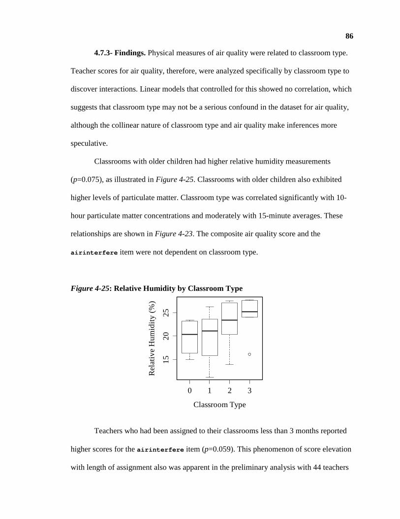
86
4.7.3- Findings. Physical measures of air quality were related to classroom type.
Teacher scores for air quality, therefore, were analyzed specifically by classroom type to
discover interactions. Linear models that controlled for this showed no correlation, which
suggests that classroom type may not be a serious confound in the dataset for air quality,
although the collinear nature of classroom type and air quality make inferences more
speculative.
Classrooms with older children had higher relative humidity measurements
(p=0.075), as illustrated in Figure 4-25. Classrooms with older children also exhibited
higher levels of particulate matter. Classroom type was correlated significantly with 10-
hour particulate matter concentrations and moderately with 15-minute averages. These
relationships are shown in Figure 4-23. The composite air quality score and the
airinterfere item were not dependent on classroom type.
Figure 4-25: Relative Humidity by Classroom Type
Teachers who had been assigned to their classrooms less than 3 months reported
higher scores for the airinterfere item (p=0.059). This phenomenon of score elevation
with length of assignment also was apparent in the preliminary analysis with 44 teachers
0 1 2 3
15
20
25
Classroom Type
Rel
ativ
e H
um
idity
(%
)

87
and occurred in several other domains of the physical environment. The difference
between airinterfere and airtot is discussed further in Chapter 5 with respect to how
the items are worded. The data suggests that the familiarity of a space to occupants may
be an important consideration when assessing satisfaction with IEQ.
The composite air quality score (airtot ) was moderately predicted by carbon
dioxide particle concentration, both 10-hour and 15-minute time-weighted averages.
Including school as a predictor increases the significance of carbon dioxide concentration
as a predictor. The relationship of 10-hour average carbon dioxide (p = 0.069) and school
to air composite scores is illustrated in Figure 4-26. The airinterfere item also was
correlated to carbon dioxide concentration, both with and without school as a regressor.
Figure 4-26: Composite Air Score by CO2 Concentration (10-Hour)
SECTION 4.8 - Lighting Results
4.8.1- Survey results. Survey items related to lighting were not reliable as a
group, with a Cronbach’s alpha of 0.49 and low correlations between them pairwise as
shown in Table 4-10. Based on relationships between lighting outcomes and predictors,
CO2-10hr TWA (ppm)
Air
Com
posi
te S
core
-2
-1
0
1
650 700 750 800 850
School A
650 700 750 800 850
School B

88
the items are hypothesized to reflect two psychological constructs that relate to electric
and natural lighting. Therefore, two composite scores are created for the lighting domain:
lighttot and naturaltot, respectively . The variables lightsat and lightprob
formed lighttot with a resulting alpha of 0.19. Variables naturalsat and
naturalprob combined into naturaltot with an alpha of 0.53. The low number of
items for each composite contributes to these low values of alpha. The resulting
composite scores are illustrated in Figure 4-27.
Table 4-10: Pearson’s Correlations of Lighting Outcome Items
Survey Item Summary Variable 1 2 3 4 5 6 Which of the following can you personally control…?
1 lightcontrol -
How satisfied are you with the electric light in your classroom?
2 Lightsat -0.16 -
Check all that apply about the electric light…: [inverted scale]
3 lightprob -0.29 0.11 -
How satisfied are you with the daylight… in your classroom?
4 naturalsat 0.25 -0.20 0.27 -
Check all that apply about the daylight…: [inverted scale] 5 naturalprob -0.14 -0.09 0.21
0.36 *
-
Does the lighting interfere with your ability to do your job? 6 lightinterfere 0.06 -0.03 -0.05
0.50 *
0.54 **
-

89
Figure 4-27: Composite Lighting Scores by School and Classroom Type
4.8.2- Measurement results. Lighting measures in the physical environment
varied significantly between schools but not between classroom types. Electric lighting is
predominantly fluorescent tube lamps in both schools, although the lighting power
density at School B is higher than at School A. The predominant fixture type at School B
is recessed troffers with parabolic lenses. School A uses predominantly volumetric
indirect recessed troffers. The classroom lighting measurements are summarized in Table
A-4 of Appendix A. Figure 4-28 represents the lighting measurements by school. The
distribution of window orientation, with south facing coded as +1, is also shown by
classroom type.
A B
-2.0
-1.0
0.0
1.0
School
Ele
ctric
Lig
ht S
core
0 1 2 3
-2.0
-1.0
0.0
1.0
Classroom Type
Ele
ctric
Lig
ht S
core
A B
-2-1
01
School
Na
tura
l Lig
ht S
core
0 1 2 3
-2-1
01
Classroom Type
Na
tura
l Lig
ht S
core

90
Figure 4-28: Lighting Characteristics by School
A B
5060
70
8090
School
Illum
inan
ce (
fc)
A B
1.0
1.5
2.0
2.5
School
Lig
htin
g P
ower
Den
sity
(W
/ft²
)
A B
2.0
2.4
2.8
School
Illum
inan
ce R
atio
A B
-0.2
0.2
0.6
School
Fra
ctio
n of
Day
Lig
hts
On
School
Orie
ntat
ion
A B
-11
0.0
0.2
0.4
0.6
0.8
1.0
Classroom Type
Orie
ntat
ion
0 1 2 3
-11
0.0
0.2
0.4
0.6
0.8
1.0

91
4.8.3- Findings. The composite electric lighting score, lighttot , was regressed
onto illuminance ratio, and school with illuminance ratio being a significant predictor (p
= 0.036). Illuminance ratio was also significant without school included as a regressor.
This relationship is illustrated in Figure 4-29. There were no other significant
relationships between the electric lighting composite score and the physical environment.
Figure 4-29: Composite Lighting Score by Illuminance Ratio
Natural light composite scores differ by school (p = 0.040), with teachers at
School A being more satisfied. Floor area and school significantly predict composite
natural light satisfaction; however, when the interaction for school and area is included,
area is not a significant predictor. The distribution of scores precludes suggestive findings
on area and school as predictors of satisfaction with natural light. This complicated
relationship is shown in Figure 4-30.
When the natural lighting composite score, naturaltot , is regressed onto
illuminance and school, illuminance is a significant predictor (p = 0.004). However,
illuminance levels do not predict satisfaction without school, which is also a significant
2.0 2.4 2.8
-2.0
-1.0
0.0
1.0
Illuminance Ratio
Ele
ctri
c L
igh
t C
om
po
site
Sco
re
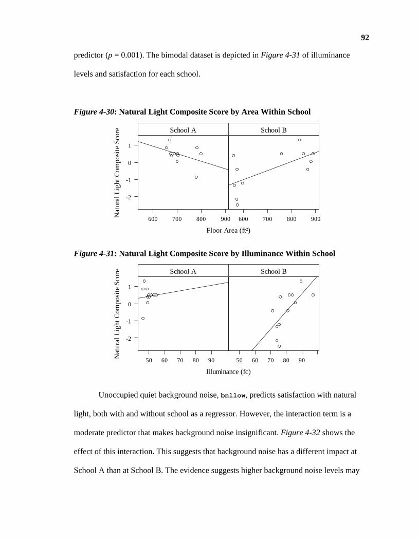
92
predictor (p = 0.001). The bimodal dataset is depicted in Figure 4-31 of illuminance
levels and satisfaction for each school.
Figure 4-30: Natural Light Composite Score by Area Within School
Figure 4-31: Natural Light Composite Score by Illuminance Within School
Unoccupied quiet background noise, bnllow , predicts satisfaction with natural
light, both with and without school as a regressor. However, the interaction term is a
moderate predictor that makes background noise insignificant. Figure 4-32 shows the
effect of this interaction. This suggests that background noise has a different impact at
School A than at School B. The evidence suggests higher background noise levels may
Floor Area (ft²)
Na
tura
l Lig
ht C
omp
osite
Sco
re
-2
-1
0
1
600 700 800 900
School A
600 700 800 900
School B
Illuminance (fc)
Na
tura
l Lig
ht C
omp
osite
Sco
re
-2
-1
0
1
50 60 70 80 90
School A
50 60 70 80 90
School B
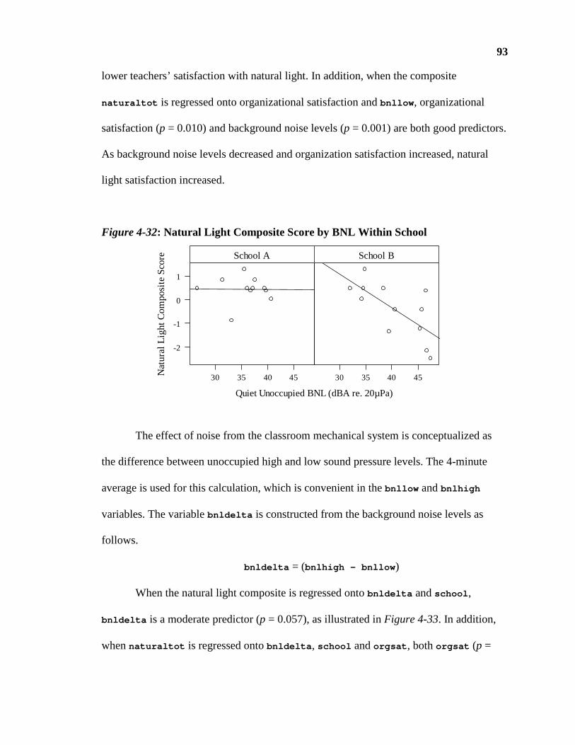
93
lower teachers’ satisfaction with natural light. In addition, when the composite
naturaltot is regressed onto organizational satisfaction and bnllow , organizational
satisfaction (p = 0.010) and background noise levels (p = 0.001) are both good predictors.
As background noise levels decreased and organization satisfaction increased, natural
light satisfaction increased.
Figure 4-32: Natural Light Composite Score by BNL Within School
The effect of noise from the classroom mechanical system is conceptualized as
the difference between unoccupied high and low sound pressure levels. The 4-minute
average is used for this calculation, which is convenient in the bnllow and bnlhigh
variables. The variable bnldelta is constructed from the background noise levels as
follows.
bnldelta = (bnlhigh – bnllow )
When the natural light composite is regressed onto bnldelta and school ,
bnldelta is a moderate predictor (p = 0.057), as illustrated in Figure 4-33. In addition,
when naturaltot is regressed onto bnldelta , school and orgsat , both orgsat (p =
Quiet Unoccupied BNL (dBA re. 20µPa)
Nat
ura
l Lig
ht C
ompo
site
Sco
re
-2
-1
0
1
30 35 40 45
School A
30 35 40 45
School B

94
0.058) and bnldelta (p = 0.064) are moderate predictors. All lighting tests are
summarized in Table B-2 and Table B-3 of Appendix B.
Figure 4-33: Natural Light Composite Score by Background Noise Delta
SECTION 4.9 - Furnishings Results
Furniture items are reliable with a Cronbach’s alpha of 0.87. Based on high
correlations, all items are included in the composite furniture score, furntot . As
presented in Table 4-2, the furnishings composite is also significantly correlated with
satisfaction in classroom size, views, acoustics and air quality. The broad IEQ composite
score, ieqT, also is related to the furniture composite score.
Difference in Unoccupied BNL (dBA)
Na
tura
l Lig
ht
Com
posi
te S
core
-2
-1
0
1
5 10 15 20
School A
5 10 15 20
School B

95
Table 4-11: Pearson’s Correlations of Furniture Outcome Items
Survey Item Summary Variable 1 2 3 4 5 6 How satisfied are you with the comfort of furniture for adults?
1 furnadult -
How satisfied are you with the comfort of furniture for children? 2 furnchild
0.46
-
How satisfied are you with .. the adjustability of furniture? 3 furnadjust
0.64 ***
0.75 ***
-
How satisfied are you with the furniture layout…? 4 furnlayout
0.57 **
0.52 **
0.74 ***
-
How satisfied are you with the colors and textures …? 5 finishes 0.28
0.48 *
0.48 *
0.53 **
-
Does the furniture interfere with your ability to do your job? 6 furninterfere
0.53 **
0.50 *
0.59 **
0.70 ***
0.57 **
-
Teachers at School A report significantly higher satisfaction with furnishings than
those at School B, as illustrated in Figure 4-34.
Figure 4-34: Furnishings Composite Score by School
Color was a significant predictor of satisfaction (p = 0.011). When the furnishings
composite score was regressed onto wall color and school, color was a moderate
predictor (p = 0.077), as plotted in Figure 4-35. Cool colors related to higher scores. In
A B
-2-1
01
School
Fu
rnis
hin
gs
Co
mp
osi
te S
core
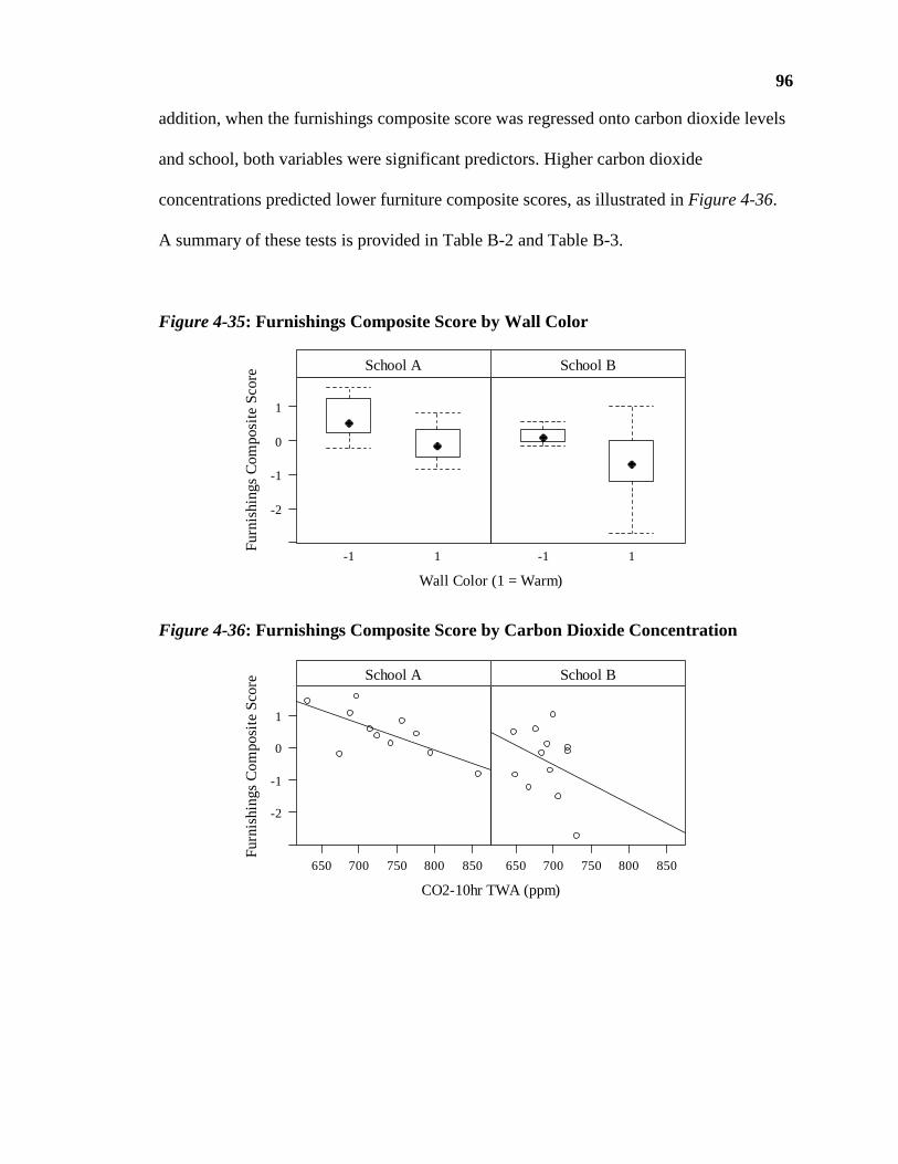
96
addition, when the furnishings composite score was regressed onto carbon dioxide levels
and school, both variables were significant predictors. Higher carbon dioxide
concentrations predicted lower furniture composite scores, as illustrated in Figure 4-36.
A summary of these tests is provided in Table B-2 and Table B-3.
Figure 4-35: Furnishings Composite Score by Wall Color
Figure 4-36: Furnishings Composite Score by Carbon Dioxide Concentration
Wall Color (1 = Warm)
Fur
nish
ings
Com
posi
te S
core
-2
-1
0
1
-1 1
School A
-1 1
School B
CO2-10hr TWA (ppm)
Fur
nish
ings
Co
mpo
site
Sco
re
-2
-1
0
1
650 700 750 800 850
School A
650 700 750 800 850
School B

97
SECTION 4.10 - Cleaning Results
Items in the cleaning domain are reliable with a Cronbach’s alpha of 0.85. The
items were correlated as indicated Table 4-12. All items were included in the composite
score, cleantot . Cleaning composite scores are significantly higher at School A than at
School B. Classroom type does not predict satisfaction with cleaning. Scores are
described in Figure 4-37.
Table 4-12: Pearson’s Correlations of Cleaning Outcome Items
Survey Item Summary Variable 1 2 3 4 5 How satisfied are you with the tidiness of your classroom?
1 cleanorg -
How satisfied are you with the cleaning service in your classroom? 2 cleanservice
0.42 *
-
How satisfied are you with the wall display surfaces? 3 cleandisplay
0.64 **
0.58 **
-
Which of the following are problems…? [inverted scale] 4 cleanprob
0.38
0.54 **
0.62 **
-
Does the cleaning and organization interfere with your ability to do your job?
5 cleaninterfere 0.53 **
0.52 *
0.53 **
0.58 **
-
Figure 4-37: Composite Cleaning Score by School and Classroom Type
A B
-1.5
-0.5
0.5
1.5
School
Cle
anin
g C
om
po
site
Sco
re
0 1 2 3
-1.5
-0.5
0.5
1.5
Classroom Type
Cle
anin
g C
om
po
site
Sco
re

98
When the cleaning composite score, cleantot , is regressed onto school and wall
color, color predicted satisfaction (p = 0.021), as illustrated in Figure 4-38. When the
composite is regressed onto school and illuminance levels, both predictors are significant.
Higher classroom illuminance values are associated with higher scores as shown in
Figure 4-39.
Figure 4-38: Cleaning Composite Score by Wall Color
Figure 4-39: Cleaning Composite Score by Illuminance
Area is also a predictor, but the effect is not significant when the interaction with
school is included as a regressor. When the cleaning composite score, cleantot , is
regressed onto area, school and interaction area Xschool , school (p = 0.009) and the
Wall Color (1 = Warm)
Cle
ani
ng C
ompo
site
Sco
re
-1
0
1
2
-1 1
School A
-1 1
School B
Illuminance (fc)
Cle
ani
ng C
ompo
site
Sco
re
-1
0
1
2
50 60 70 80 90
School A
50 60 70 80 90
School B
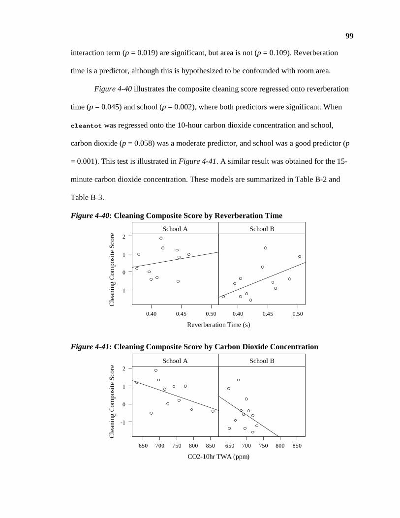
99
interaction term (p = 0.019) are significant, but area is not (p = 0.109). Reverberation
time is a predictor, although this is hypothesized to be confounded with room area.
Figure 4-40 illustrates the composite cleaning score regressed onto reverberation
time (p = 0.045) and school (p = 0.002), where both predictors were significant. When
cleantot was regressed onto the 10-hour carbon dioxide concentration and school,
carbon dioxide (p = 0.058) was a moderate predictor, and school was a good predictor (p
= 0.001). This test is illustrated in Figure 4-41. A similar result was obtained for the 15-
minute carbon dioxide concentration. These models are summarized in Table B-2 and
Table B-3.
Figure 4-40: Cleaning Composite Score by Reverberation Time
Figure 4-41: Cleaning Composite Score by Carbon Dioxide Concentration
Reverberation Time (s)
Cle
ani
ng C
ompo
site
Sco
re
-1
0
1
2
0.40 0.45 0.50
School A
0.40 0.45 0.50
School B
CO2-10hr TWA (ppm)
Cle
ani
ng C
omp
osite
Sco
re
-1
0
1
2
650 700 750 800 850
School A
650 700 750 800 850
School B

100
SECTION 4.11 - Global IEQ Results
4.11.1- Survey results. This study uses three scores to represent global IEQ
satisfaction. The most basic is from the last item on the survey, ieqoverall , which
reads, “All things considered, how satisfied are you with your classroom?” The semantic
differential scale for this item is coded 1 through 6, and all participants responded at the
levels of 4, 5, or 6, as listed in Table B-1. The other two global IEQ scores are
composites created from the domain composite scores that are described in the sections
above. A broad global score, ieqT , combined all the domain composites by first
converting them to z scores, thereby providing equal weight to each. Therefore, this
broad global score combined nine domain composites, or 30 survey items, listed in Table
4-1. The third measure of global IEQ quality targeted the sensory environment,
ieq.sensory . This score was created from the five domain composites: accsat2 ,
thermsat , airtot , lighttot and naturaltot . Therefore, ieq.sensory represents 14
survey items. Score distributions are presented in Figure 4-42.
Figure 4-42: Score Distribution for IEQ Overall Measures
None of the global IEQ scores differed significantly between schools, although
the broad IEQ composite, ieqT, was most different (p = 0.066). The score distributions
are shown in Figure 4-42. The overall IEQ item is significantly correlated with ieqT (r =
A B
-1.0
0.0
1.0
School
Item
ieqo
vera
ll
A B
-2-1
01
School
Sen
sory
IE
Q C
ompo
site
Sco
re (
5)
A B
-2-1
01
School
Bro
ad
IEQ
Com
posi
te S
core
(9)

101
0.48) but not with ieq.sensory (r = 0.32). When the item ieqoverall was regressed
onto ieqT and school , ieqT was still a significant predictor (p = 0.024). This suggests
that when answering about overall classroom satisfaction, teachers include considerations
beyond just the acoustic, lighting, thermal and respiratory conditions. Because the two
composite global IEQ scores share five domain composites, they are significantly related
to each other (r = 0.89). Table 4-13 lists the correlations between the three IEQ survey
scores, and Figure 4-43 illustrates the relationship between the item ieqoverall and
both IEQ composite scores.
Table 4-13: Pearson’s Correlation of IEQ Scores
IEQ Item Variable 1 2 3 All things considered, how satisfied are you with your classroom?
1 ieqoverall -
Composite of accsat2 , thermsat , airtot , lighttot , and naturaltot
2 ieq.sensory 0.32
-
Composite of sizesat , viewsat , accsat2 , thermsat , airtot , lighttot , naturaltot , furntot , cleantot
3 ieqT 0.48
* 0.89 ***
-
Figure 4-43: Item ieqoverall by IEQ Composite Scores
-2 -1 0 1
-1.0
0.0
1.0
2.0
Broad IEQ Composite Score (9)
Item
ieq
ove
rall
-2 -1 0 1
-1.5
-0.5
0.5
1.5
Sensory IEQ Composite Score (5)
Item
ieq
ove
rall

102
Each of the three global IEQ scores were tested for relationships with teacher
characteristics including age, experience, length of assignment to classroom, title and
organizational satisfaction. When the IEQ overall item was regressed onto organizational
satisfaction composite score and school, orgsat was a moderate predictor (p = 0.086).
This test is listed in Table B-3. Other teacher characteristics were not correlated with the
scores.
4.11.2- Findings. Of the three global IEQ scores, the broad composite ieqT was
related most to measurements in the physical environment, while the single item
ieqoverall showed the fewest relationships. For tests with ieqoverall , orgsat was
included in the compact model and school was not. This is because orgsat was a good
predictor of ieqoverall , while scores did not vary significantly between schools as
discussed above. When the item ieqoverall is regressed onto orgsat and plants , both
orgsat (p = 0.023) and plants (p = 0.049) are significant predictors. Similarly, when
ieqoverall is regressed onto carpet and orgsat , carpet is a moderate predictor (p =
0.076), and orgsat is a significant predictor (p = 0.050). There was also a relationship
between thermal comfort and the ieqoverall item. When ieqoverall was regressed
onto orgsat and relative humidity, relative humidity was a significant predictor (p =
0.043). These tests are summarized in Table B-2 and Table B-3.
Findings for the two composite IEQ scores ieqT and ieq.sensory are discussed
together. When the sensory IEQ composite, ieq.sensory, was regressed onto area and
school , area was a significant predictor (p = 0.021). When the broad IEQ composite,
ieqT, was regressed onto area and school , both area (p = 0.005) and school (p =
0.036) were significant predictors. When the interaction term was included in the model

103
for ieqT , it was not significant. The bimodal nature of floor area at School B and the
corresponding difference in teacher satisfaction helps describe this result, since both
scores and area within School A do not vary as widely. This is illustrated in Figure 4-44.
Figure 4-44: Area by IEQ Scores Within School
There were several relationships between acoustics and composite IEQ scores.
When the sensory IEQ composite, ieq.sensory, was regressed onto quiet unoccupied
background noise levels (bnllow) and school, bnllow was a moderate predictor (p =
0.074). While this relationship is present at School A, a group of low scores at school B
in rooms with high unoccupied, A-weighted background noise levels around 45 dB re 20
µPa makes the effect more pronounced, as illustrated in Figure 4-45. There is a similar
Floor Area (ft²)
Se
nsor
y IE
Q C
omm
pos
ite S
core
(5)
-2
-1
0
1
600 700 800 900
School A
600 700 800 900
School B
Floor Area (ft²)
Bro
ad
IEQ
Co
mm
pos
ite S
core
(9)
-2
-1
0
1
600 700 800 900
School A
600 700 800 900
School B

104
relationship to the broad IEQ composite. When the composite ieqT was regressed onto
quiet unoccupied background noise levels and school, bnllow was a significant predictor
(p = 0.046). When ieqT was regressed onto quiet unoccupied background noise levels
and school, including the interaction bnllow Xschool , only the interaction term was a
moderate predictor (p = 0.083). This suggests stronger differences between schools in the
effect of background noise levels on teacher satisfaction. That the average A-weighted
bnllow of School B is a significant 4.6 dB higher than that of School A is a consideration
in interpreting this result.
Figure 4-45: Unoccupied Quiet BNL by IEQ Scores Within School
Quiet Unoccupied BNL (dBA re. 20µPa)
Se
nsor
y IE
Q C
omm
posi
te S
core
(5)
-2
-1
0
1
30 35 40 45
School A
30 35 40 45
School B
Quiet Unoccupied BNL (dBA re. 20µPa)
Bro
ad
IEQ
Co
mm
pos
ite S
core
(9)
-2
-1
0
1
30 35 40 45
School A
30 35 40 45
School B

105
The relationships between teacher IEQ satisfaction and quiet unoccupied
background noise level (bnllow ) are similar to those of loud background noise level
(bnlhigh ). The average A-weighted bnlhigh measurement at School A is about 1 dB
higher than at school B, an insignificant difference as noted in Table A-3. When the
sensory IEQ composite score, ieq.sensory, is regressed onto bnlhigh and school ,
bnlhigh is a moderate predictor (p = 0.057). The interaction of bnlhigh Xschool is not
significant when added to the model. When the broad IEQ composite score, ieqT, is
regressed onto bnlhigh and school , bnlhigh is a moderate predictor (p = 0.084), and
school is a significant predictor (p = 0.046). However, when ieqT is regressed onto
bnlhigh , school and the interaction bnlhigh Xschool , only school and the interaction
term are significant. This suggests that the background noise of mechanical systems has a
bigger negative impact on teacher IEQ satisfaction at School B than at School A. This is
illustrated in Figure 4-46.
Figure 4-46: Unoccupied Loud BNL by Broad IEQ Score Within School
Reverberation time is related to IEQ satisfaction, although this finding may be
due to the confound of area with reverberation time. When the broad IEQ composite
Loud Unoccupied BNL (dBA re. 20µPa)
Bro
ad
IEQ
Co
mm
pos
ite S
core
(9)
-2
-1
0
1
40 45 50 55
School A
40 45 50 55
School B

106
score, ieqT, was regressed onto reverberation time and school, both rt20 (p = 0.030)
and school (p = 0.018) were significant predictors. Higher reverberation times were
associated with higher scores. When the sensory IEQ composite score, ieq.sensory,
was regressed onto reverberation time and school, both rt20 was a moderate predictor (p
= 0.089).
There was no effect of particulate matter concentrations on IEQ composite scores.
The suspended dust in classrooms varied most by classroom type. When the effect of
classroom type was included in the regression, there was still no effect on teacher scores.
Relative humidity predicted the sensory IEQ composite score and was a moderate
predictor of the broad IEQ composite score. When ieq.sensory was regressed onto
rh10 and school , rh10 was significant with p = 0.033 as illustrated in Figure 4-47.
When ieqT was regressed onto rh10 and school , both rh10 (p = 0.090) and school (p =
0.085) were moderate predictors. These tests are provided in Table B-3. This suggests
that the sensory IEQ composite score may be less sensitive to differences between
schools than the broad IEQ composite score.
Figure 4-47: Composite Sensory IEQ Score by Relative Humidity
Relative Humidity (%)
Se
nsor
y IE
Q C
omm
posi
te S
core
(5)
-2
-1
0
1
15 20 25
School A
15 20 25
School B

107
The average high electric lighting levels in a classroom correlate with teacher
satisfaction, with more illuminance matched with higher scores. The two schools were
significantly different in illuminance levels, with School B measuring on average 30.9
footcandles more than School A, as described in Appendix A, Table A-4. When the
sensory IEQ composite, ieq.sensory, was regressed onto illuminance levels and
school, illum (p = 0.099) and school (p = 0.064) were both moderate predictors. When
the broad IEQ composite, ieqT , was regressed onto illuminance levels and school, illum
(p = 0.015) and school (p = 0.004) were both significant predictors. These tests are listed
in Table B-3 and illustrated in Figure 4-48. The broad IEQ score was more related to
classroom illuminance levels than was the sensory IEQ score, suggesting that items
related to satisfaction with area, size, cleaning and furnishings are impacted by lighting
levels.
Higher illuminance ratios in classrooms related to higher teacher IEQ scores for
both IEQ composites. When the sensory IEQ composite, ieq.sensory , was regressed
onto illuminance ratio and school, illumratio was a significant predictor (p = 0.014).
When the broad IEQ composite, ieqT , was regressed onto illuminance ratio and school,
illumratio (p = 0.018) and school (p = 0.038) were both significant predictors. These
tests are listed in Table B-3 and illustrated in Figure 4-48.

108
Figure 4-48: Illuminance and Illuminance Ratio by IEQ Scores Within School
Color is a moderate predictor of ieqT but not when school is included as a
regressor. When ieqT is regressed onto color and classroom type, color is a significant
predictor (p = 0.032). The number of hiding spaces in a classroom was negatively
correlated with ieqT , although this was not significant with school included in model.
The fraction of permanent carpet in rooms predicts the sensory IEQ composite score with
school included as a regressor. For the broad IEQ composite, carpet is a moderate
predictor. In both cases, a greater fraction of permanent carpet corresponded with lower
IEQ satisfaction scores. These findings, listed in Table B-3, may be the result of another
Illuminance (fc)
Bro
ad
IEQ
Co
mm
pos
ite S
core
(9)
-2
-1
0
1
50 60 70 80 90
School A
50 60 70 80 90
School B
Illuminance Ratio
Bro
ad
IEQ
Co
mm
pos
ite S
core
(9)
-2
-1
0
1
2.0 2.5 3.0
School A
2.0 2.5 3.0
School B

109
variable confounded with carpet type, such as room area or classroom type. These
confounds are illustrated in Figure 4-49.
Figure 4-49: Confounds with Carpet
SECTION 4.12 - Summary
The teacher survey generated the outcome measure for this study with items
combined to form composite scores for each domain. These composites also were
combined and further analyzed as a measure of global IEQ. All of the statistical tests are
listed in Table B-2 of Appendix B. Table B-3 also includes the output of statistical
analysis from the R software employed. A summary of the findings that represent strong
patterns in the data is provided in Table 4-14, organized by domain composite score. As a
measure of the internal structure of the survey, each composite score also is compared to
the item ieqoverall in this table using Spearman’s rho. Results reinforce the
correlations calculated in Table 4-2, with view, size and cleaning composite scores
strongly related to the item ieqoverall .
550 650 750 850
0.1
0.3
0.5
Floor Area (ft²)
Fra
ctio
n o
f C
arp
et
0 1 2 3
0.1
0.3
0.5
Classroom Type
Fra
ctio
n o
f C
arp
et

110
Table 4-14: Composite Score Summary
Composite Score
Notable Predictive Tests [significance: p < 0.10 & p < 0.05]
Spearman’s rho (ρ) to ieqoverall (p
value)
sizesat area + school, bnllow + school, bnllow + crtype + schoolXcrtype
0.517 (0.011)
viewsat illumratio + school 0.531 (0.009)
accsat2 area + school, bnllow + school, bnlhigh + school, rh10 + school
0.238 (0.274)
thermsat color + crtype, orient.factor + crtype 0.057 (0.795)
airtot co210 + school, co215 + school, onoff10 + school
0.157 (0.486)
lighttot illumratio + school 0.219 (0.316)
naturaltot illum + school, bnllow + school, bnllow + school + bnllowXschool, bnllow + school + orgsat, bnldelta + orgsat
0.364 (0.088)
furntot color + school, co210 + school, co215 + school
0.252 (0.247)
cleantot area + school + areaXschool, color + school, co210 + school, co215 + school
0.492 (0.017)
ieq.sensory
area + school, carpet + school, bnllow + school, bnlhigh + school, illum + school, illumratio + school, rh10 + school
0.397 (0.067)
ieqT
area + school, carpet + school, bnllow + school, rh10 + school bnlhigh + school + bnlhighXschool illum + school, illumratio + school, color + crtype
0.576 (0.005)
ieqoverall orgsat, plants + orgsat 1.000 (N/A)

111
CHAPTER 5 - Discussion
As with other places of employment, the physical environment of early learning
schools impacts the behavior of occupants. Following the framework presented in
Chapter 1, this study contributes to the literature on early education and IEQ in several
ways. As detailed in Chapter 4, findings show the physical environment does predict
teacher satisfaction scores with IEQ on a self-reported assessment. Further, the study
suggests that organizational satisfaction may mediate satisfaction with IEQ. A third
contribution of this study is insight into the reliability and validity of the survey tool
developed for this study in assessing IEQ, as currently understood in the literature.
SECTION 5.1 - Physical Environment and IEQ Satisfaction
The study strongly suggests that the physical environment predicts teacher
satisfaction with IEQ. The picture that emerges from the findings shows complex
relationships between overall satisfaction and satisfaction with various sensory domains.
Additionally, measurements from one domain in the physical environment often
predicted IEQ satisfaction in a different domain. This finding supports Humphrey’s
(2005) observations regarding the complexities of forming a unitary IEQ index that
would be applicable for various populations and different building users.
SECTION 5.2 - Organizational Satisfaction and IEQ Satisfaction
Structural and symbolic variables are intertwined (Cheryan et al., 2014). This
study suggests that classroom features such as color can be as important to occupant
satisfaction as the temperature. In addition, the general composite score, which

112
aggregates satisfaction with furnishing and finishes, is predicted by several domains in
the physical environment, suggesting that the lighting and background noise can
influence perception of the general accommodations in a classroom. Similarly, the broad
IEQ composite score was predicted by more measurements in the physical environment
than was the targeted sensory IEQ composite score.
SECTION 5.3 - Survey Structure and Discussion
Preliminary analysis with all 44 participants suggested that teachers’ satisfaction
scores were dependent on teacher characteristics, such as organizational satisfaction, age
and length of time teachers had been assigned to the same room. While these teacher-
level characteristics were moderately predictive of some items in the final analysis with
23 teachers, the relationships were not as suggestive or broad in effect on satisfaction
items. The sample selected of 18 Lead Teachers and 5 Assistant Teachers intentionally
excluded teachers with lower titles who also generally reported lower scores. In addition
to the loss of power, this loss of variance in scores may be one reason teacher
characteristics were less suggestive of scores in the final analysis.
Teachers with less organizational status may respond differently to interventions
in the physical environment than teachers in more established positions. For example,
Teacher’s Aides may be more satisfied if their classroom assignments change more
frequently than would teachers with more tenure. The correspondence between
organizational satisfaction and IEQ satisfaction also suggests that interventions in the
physical environment may improve employee engagement for teachers with less status.

113
Grouping behavioral items into composite scores is an important feature of this
study. Correlations between teacher responses and the physical environment tended to
remain when the items were grouped with other items. For example, illuminance was a
strong predictor for the naturalsat item on the survey, which is aggregated into
naturaltot that also correlated to illuminance. This composite is grouped further into
the broad composite IEQ score, ieqT , which is also predicted by illuminance. In contrast,
no emergent relationships are obvious because of aggregating items. Therefore, the
composite score did not appear to create a more accurate measure of occupant behavior
as predicted by the physical environment.
An important feature of the study methodology is that items were excluded to
improve the predictive power of the physical environment. In addition, five of the
composite scores included an item that was worded to reflect occupant performance as
opposed to occupant satisfaction. For example, the item airinterfere was worded
“Does the air quality interfere with your ability to do your job?” while the more typical
item airsat was worded “How satisfied are you with the air quality in your classroom?”
In the case of air quality, these items appeared to be measuring different yet meaningful
psychological constructs based on the predictive power of the physical environment. The
fact that selection based on Cronbach’s alpha eliminated three of the eight “performance”
items is further evidence that item wording is an important consideration is structuring
IEQ satisfaction items.
When analyzing the agreement of different teachers in the same classroom,
another issue arises concerning the definition of reliability. Reliability can be defined in
the sense of inter-rater reliability, where the focus of analysis is how well different

114
teachers agree in assessing the same classroom environment. Alternatively, a focus on
intra-rater agreement considers how well a specific teacher observes differences in a
classroom environment based on individual characteristics. While subtle, this distinction
is analogous to the discussion of the dual purposes occupant surveys serve in the
literature. Surveys can view occupants as a diagnostic instrument for fine-tuning building
systems or, alternatively, target human behavior, with the physical environment
conceptualized as a mediator of behavior. Regarding data analysis for the present study,
the decision to select teachers to represent classrooms, instead of averaging teacher
scores, is based on the latter approach of organizing the analysis around occupants, as
opposed to environmental control systems.
SECTION 5.4 - IEQ Weightings
Heinzerling et al. (2013) reviewed the literature for various weighting schemes of
occupant satisfaction with sensory domains. They formed weightings by creating a model
that links items within a survey assessment to each other by using multivariate
regressions, with overall satisfaction as the outcome measure. For comparison to their
findings, a similar model is presented in Table 5-1 that regressed the ieqoverall item
onto the sensory domain composite scores of accsat2 , airtot , lighttot , naturaltot
and thermsat . The column for lighting includes both composite scores for electric light
and natural light used for this study. In contrast to the Heinzerling et al. study, results
show that lighting was more predictive than acoustics of the overall IEQ item on the
survey. Acoustics and air quality had approximately equal weight. Satisfaction with
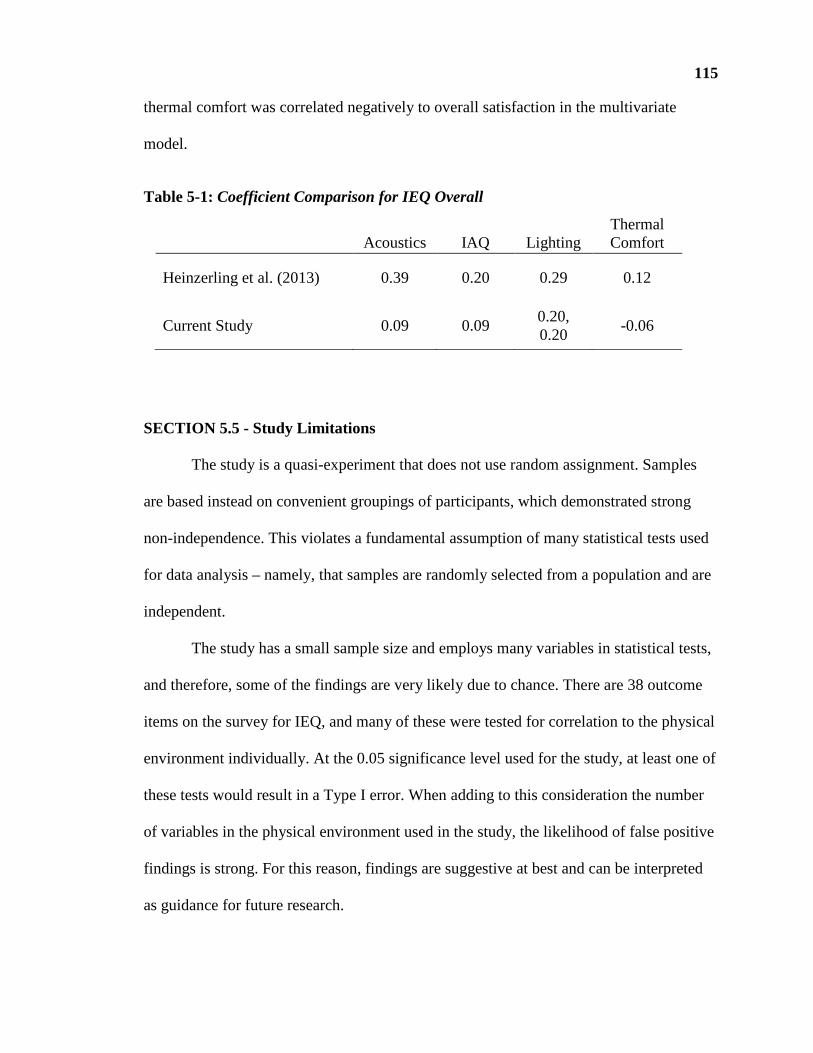
115
thermal comfort was correlated negatively to overall satisfaction in the multivariate
model.
Table 5-1: Coefficient Comparison for IEQ Overall
Acoustics IAQ Lighting Thermal Comfort
Heinzerling et al. (2013) 0.39 0.20 0.29 0.12
Current Study 0.09 0.09 0.20, 0.20
-0.06
SECTION 5.5 - Study Limitations
The study is a quasi-experiment that does not use random assignment. Samples
are based instead on convenient groupings of participants, which demonstrated strong
non-independence. This violates a fundamental assumption of many statistical tests used
for data analysis – namely, that samples are randomly selected from a population and are
independent.
The study has a small sample size and employs many variables in statistical tests,
and therefore, some of the findings are very likely due to chance. There are 38 outcome
items on the survey for IEQ, and many of these were tested for correlation to the physical
environment individually. At the 0.05 significance level used for the study, at least one of
these tests would result in a Type I error. When adding to this consideration the number
of variables in the physical environment used in the study, the likelihood of false positive
findings is strong. For this reason, findings are suggestive at best and can be interpreted
as guidance for future research.

116
SECTION 5.6 - Implications for Building Users
In this study, many of the classrooms were scored by 2 or 3 teachers. The
consistency of different raters is sometimes evaluated with a Fleiss Kappa test that
returns 1 for total agreement and 0 for no agreement. When treated as raters of an
objective domain, teacher performance was marginal with Fleiss Kappa of around 0.40.
Using surveys as efficient ways to measure the environment has a proven record of
accomplishment, although it is clear that such readings have significant “noise” from
individual and group differences.
One of the questions this study asks is whether the survey tools can be
conceptualized instead in the tradition of response-to-intervention, where they are viewed
as one feature of a larger program that seeks to create optimal outcomes at the individual
level. With the maturity of wirelesses sensor networks for commercial market, the
concept of individualized comfort settings in open spaces is within reach. Anecdotally,
one of the most sensitive sensory domains, acoustics, is treated commonly with
earphones that selectively and wirelessly create soundscapes for occupants.
Researchers can conceptualize occupant surveys as a target construct in
themselves, as opposed to indicators of the physical environment. While safe limits for
the physical environment are a basic responsibility of designers, precisely describing
target tolerances for each sensory domain may be less important to occupants than
understanding the impact of change across sensory domains. For example, models of IEQ
quality could conceptualize the rate of change in sensory domains as opposed to target
ranges for each domain. Higher quality IEQ environments may be imagined to respond
faster or slower to occupants' behavior and expressed desires.

117
Study findings suggest that satisfaction with the physical environments cannot be
reduced to measurable variables in the physical environment. Instead, the way teachers
use their classrooms in a social context is the best way to appraise their satisfaction with
their classrooms. The practical opportunity suggested is that building users and designers
are as accountable to building occupants as they are to budgets. More tenuously,
designers have reason to suspect that engaging users in discussions about how they would
like to interact with their sensory environment could translate into increased program
outcomes, be they productivity, learning, sales or satisfaction.
SECTION 5.7 - Implications for Designers
This study shows that engineers and architects can address teachers’ satisfaction
with IEQ through design. Specifically, occupant surveys present a key strategy for
improving IEQ. As demonstrated by the survey developed for this study, the value of
responses is strongly related to the selection and wording of survey items. In addition,
items can be grouped meaningfully into composite scores and retain much of their
predictive power for quality in the physical environment. While it may be impossible to
create a useful score related to combinations of variables in the physical environment, the
perception of IEQ appears to be more unitary, with composite scores better reflecting
satisfaction in the sensory domains.
118
CHAPTER 6 - Summary
This project compared physical measurements from classrooms at two early
learning schools to teachers’ self-reported satisfaction with IEQ. Forty-four teachers
participated from twenty-three different classrooms, with some teachers reporting on the
same classroom. Physical measures included unoccupied and occupied sound pressure
level, reverberation time, occupied carbon dioxide and particulate matter concentrations,
occupied temperature and relative humidity, and illuminance levels at one position at the
ceiling. Various characteristics of the rooms were included such as floor area, floor
covering, wall colors and the ability to separate the room from adjacent spaces.
Teacher characteristics such as time assigned to the same room, organizational
satisfaction and school assignment all mediate satisfaction with the classroom IEQ.
Findings show that unoccupied background noise levels, illuminance levels and floor area
in the classroom are good predictors of overall satisfaction. Other predictors include
classroom orientation, the color of the walls and average carbon dioxide concentration.
An overall satisfaction score that combined several sensory domain composite scores was
related strongly to the single survey item “All things considered, how satisfied are you
with your classroom?”
Satisfaction with classroom size was predicted by floor area and unoccupied
sound pressure level. Satisfaction with views was predicted by illuminance ratio, and
satisfaction with acoustics was predicted by unoccupied background noise levels, noise
level of mechanical equipment and relative humidity. Thermal comfort was predicted by
classroom orientation and wall color, while satisfaction with air quality was predicted by
carbon dioxide concentrations. Satisfaction with the electric lighting was predicted by

119
illuminance ratio. Satisfaction with natural lighting was predicted by average illuminance
and several measurements from the acoustic domain. Satisfaction with furnishings was
predicted by wall color and carbon dioxide concentration, while satisfaction with
cleaning correlated to illuminance, wall color and carbon dioxide concentration.
The survey tool revealed strong correlations between satisfaction levels of
different sensory domains, such as temperature and acoustics and lighting and air quality.
Self-reported satisfaction with overall IEQ was related to a broad composite score that
combined 30 other survey items, supporting construct validity of the tool. This broad
composite score exhibited more significant relationships to measures of the physical
environment than a targeted sensory IEQ composite score.
The study does not feature random assignment and uses convenient samples that
demonstrated strong non-independence. The study has a relatively small sample size and
employs many variables in statistical tests, and therefore, some of the findings are very
likely due to chance. Nonetheless, findings are strongly suggestive that differences in the
physical environment correspond to satisfaction with IEQ. This intuitive finding lends
support to the theory that quality in the physical environment affects program outcomes.
The study also confirms that organizational satisfaction mediates satisfaction with IEQ,
suggesting that the reverse may also be true.

120
REFERENCES
Abdou, O. A. (1997). Effects of luminous environment on worker productivity in
building spaces. Journal of Architectural Engineering, 3(3), 124-132.
American Educational Research Association [AERA], American Psychological
Association, & National Council on Measurement in Education. (1999).
Standards for educational and psychological testing. Washington: AERA.
American National Standards Institute [ANSI]. (2010). American National Standard
acoustical performance criteria, design requirements, and guidelines for schools,
part 1: Permanent schools (ANSI/ASA S12.60-2010/Part 1). New York: ANSI.
American Society of Heating Refrigerating and Air-Conditioning Engineers, Inc.
[ASHRAE]. (2004). Thermal comfort conditions for human occupancy (ANSI /
ASHRAE Standard 55-2004). Atlanta: ASHRAE.
American Society of Heating Refrigerating and Air-Conditioning Engineers, Inc.
[ASHRAE]. (2013). Ventilation for acceptable indoor air quality (ANSI /
ASHRAE Standard 62.1-2013). Atlanta: ASHRAE.
American Society of Heating Refrigerating and Air-Conditioning Engineers, Inc.
[ASHRAE], US Green Building Council, & The Chartered Institution of Building
Service Engineers. (2010). Performance measurement protocols for commercial
buildings. Atlanta: ASHRAE.
Aries, M., Aarts, M., & van Hoof, J. (2015). Daylight and health: A review of the
evidence and consequences for the built environment. Lighting Research and
Technology, 47, 6-27.
Arup. (2015). BUS methodology [website]. Retrieved from
http://www.busmethodology.org/
Bailey, J.A. (2009). A synthesis of studies pertaining to building conditions, student
achievement, student behavior, and student attitude (Unpublished doctoral
dissertation). Virginia Polytechnic Institute and State University, Virginia Beach,
VA.
Bargh, J. A., & Shalev, I. (2012). The substitutability of physical and social warmth in
daily life. Emotion, 12(1), 154.

121
Benfield, J. A., Rainbolt, G. A., Bell, P. A., & Donovan, G. (2015). Classrooms with
nature views: evidence of different student perceptions and behaviors.
Environment and Behavior, 47(2), 140-157.
Brager, G., & Baker, L. (2009). Occupant satisfaction in mixed-mode buildings. Building
Research and Information, 37, 369-380.
Bronfenbrenner, U. (1979). The ecology of human development: Experiments by nature
and design. Cambridge, Mass.: Harvard University Press.
Bronsema, B., Björck, M., Carrer, P., Clausen, G., Fitzner, K., Flatheim, G., ... &
Witterseh, T. (2004). Performance criteria of buildings for health and comfort
(Report of International Society of Indoor Air Quality and Climate [ISIAQ]-
International Council for Research and Innovation in Building and
Construction [CIB] Task Group TG 42, CIB Number 192). Rotterdam, The
Netherlands: CIB.
Buckley, J., Schneider, M., & Shang, Y. (2004). The effects of school facility quality on
teacher retention in urban school districts. Washington: National Clearinghouse
for Educational Facilities.
Bullock, C. C. (2007). The relationship between school building conditions and student
achievement at the middle school level in the commonwealth of Virginia
(Unpublished doctoral dissertation). Virginia Polytechnic Institute and State
University, Blacksburg, Va.
Burchinal, M. R., Roberts, J. E., Riggins, R., Jr., Zeisel, S. A., Neebe, E., & Bryant, D.
(2000). Relating quality of center-based childcare to early cognitive and language
development longitudinally. Child Development, 71(2), 339-357.
Burger, K. (2010). How does early childhood care and education affect cognitive
development? An international review of the effects of early interventions for
children from different social backgrounds. Early Childhood Research Quarterly,
25(2), 140-165.
Carlopio, J. R. (1996). Construct validity of a physical work environment satisfaction
questionnaire. Journal of Occupational Health Psychology, 1(3), 330-344.

122
Cassidy, D. J., Hestenes, L. L., Hegde, A., Mims, S., & Hestenes, S. (2005).
Measurement of quality in preschool child care classrooms: An exploratory and
confirmatory factor analysis of the Early Childhood Environment Rating Scale—
Revised. Early Childhood Research Quarterly, 20(3), 345-360.
Center for the Built Environment. (2004). Occupant survey report. Retrieved from
http://www.cbe.berkeley.edu/research/survey.htm
Cho, E., & Kim, S. (2015). Cronbach’s coefficient alpha: Well known but poorly
understood. Organizational Research Methods, 18(2), 207-230.
Clausen, G., & Wyon, D. P. (2008). The combined effects of many different indoor
environmental factors on acceptability and office work performance. HVAC&R
Research, 14, 103-113.
Clements-Croome, D. J. (2013). Environmental health and well-being in buildings. In D.
J. Clements-Croome (Ed.), Intelligent buildings (2nd ed., pp. 43-60). London: ICE
Publishing.
Clements-Croome, D. J., Awbi, H. B., Bakó-Biró, Z., Kochhar, N., & Williams, M.
(2008). Ventilation rates in schools. Building and Environment, 43(3), 362-367.
Cobb, E. (2004). The ecology of imagination in childhood. Putnam, Conn.: Spring.
(Original work published 1977)
Cohen, R.J., Swerdlik, M., & Sturman, E. (2013). Psychological testing and assessment:
An introduction to tests and measurement (8th ed.). New York: McGraw-Hill
Higher Education.
Cryer, D. (1999). Defining and assessing early childhood program quality. The Annals of
the American Academy of Political and Social Science, 563(1), 39-55.
Davis, M. C., Leach, D. J., & Clegg, C. W. (2011). The physical environment of the
office: Contemporary and emerging issues. In G. P. Hodgkinson & J. K. Ford
(Eds.), International review of industrial and organizational psychology (Vol.
26, pp. 193-237). Hoboken, N.J.: Wiley-Blackwell.
de Dear, R. J. (2011). Revising an old hypothesis of human thermal perception:
Alliesthesia. Building Research and Information 39(2), 108-117.

123
de Dear, R. J., Akimoto, T., Arens, E. A., Brager, G., Candido, C., Cheong, K. W. D., ...
& Zhu, Y. (2013). Progress in thermal comfort research over the last twenty
years. Indoor Air, 23(6), 442-461.
de Korte, E. M., Spiekman, M., Hoes-van Oeffelen, L., Zande, B. van der, Vissenberg,
G., Huiskes, G., & Kuijt-Evers, L. F. M. (2015). Personal environmental control:
Effects of pre-set conditions for heating and lighting on personal settings, task
performance, and comfort experience. Building and Environment, 86, 166-176.
Dickinson, D. K. (2006). Toward a toolkit approach to describing classroom quality.
Early Education and Development, 17(1), 177-202.
DiLaura, D. L., Houser, K. W., Mistrick, R. G., & Steffy, G. R. (Eds.). (2011). The
lighting handbook (10th ed.). New York: Illuminating Engineering Society of
North America.
Dutt, I. (2012). School design and students’ relationships with the natural world.
Children, Youth and Environments, 22(1), 198-226.
Dykes, C., & Baird, D. (2013). A review of questionnaire-based methods used for
assessing and benchmarking indoor environmental quality. Intelligent Buildings
International, 5(3), 135-149.
Essa, E. L., & Burnham, M. M. (2001). Childcare quality: A model for examining
relevant variables. In C. Reifel & M. H. Brown (Eds.), Early education and care,
and reconceptualizing play (Vol. 11, pp. 59-113). Oxford, England: Elsevier
Science Ltd.
European Committee for Standardization [CEN]/Technical Committee [TC] 156-
Ventilation for Buildings. (1998). Ventilation for buildings: Design criteria for
the indoor environment (Tech. Rep. CR 1752). Brussels: CEN.
Evans, G. W. (2006). Child development and the physical environment. Annual Review
of Psychology, 57, 423-451.
Fisk, W. J., Black, D., & Brunner, G. (2011). Benefits and costs of improved IEQ in US
offices. Indoor Air, 21, 357-367.
Foarde, K., & Berry, M. (2004). Comparison of bio contaminant levels associated with
hard vs. carpet floors in nonproblem schools: Results of a yearlong study. Journal
of Exposure Analysis and Environmental Epidemiology, 14, S41-S48.

124
Frontczak, M. J., & Wargocki, P. (2011). Literature survey on how different factors
influence human comfort in indoor environments. Building and Environment,
46(4), 922-937.
Goelman, H., Forer, B., Kershaw, P., Doherty, G., Lero, D., & LaGrange, A. (2006).
Towards a predictive model of quality in Canadian childcare centers. Early
Childhood Research Quarterly, 21(3), 280-295.
Gordon, R. A., Fujimoto, K. A., Kaestner, R., Korenman, S., & Abner, K. (2013). An
assessment of the validity of the ECERS-R with implications for measures of
childcare quality and relations to child development. Developmental Psychology,
49(1), 146-160.
Haghighat, F., & Donnini, G. (1999). Impact of psychosocial factors on perception of the
indoor air environment studies in 12 office buildings. Building and Environment,
34, 479-503.
Hanford, N., & Figueiro, M. (2013). Light therapy and Alzheimer's disease and related
dementia: Past, present, and future. Journal of Alzheimer's Disease, 33(4), 913-
922.
Haverinen-Shaughnessy, U., Moschandreas, D. J., & Shaughnessy, R. J. (2011).
Association between substandard classroom ventilation rates and students'
academic achievement. Indoor Air, 21(2), 121-31.
Hedge, A., & Gaygen, D. E. (2010). Indoor environment conditions and computer work
in an office. HVAC&R Research, 16(2), 123-138.
Heinsohn, R. J., & Cimbala, J. M. (2003). Indoor air quality engineering: Environmental
health and control of indoor pollutants. New York ; Basel: Marcel Dekker.
Heinzerling, D., Schiavon, S., Webster, T., & Arens, E. (2013). Indoor environmental
quality assessment models: A literature review and a proposed weighting and
classification scheme. Building and Environment, 70, 210-222.
Heschong, L. (2003). Daylighting in schools: Reanalysis report (California Energy
Commission [CEC] Publication Number 500-03-082, Attachment 3). Sacramento,
Calif.: CEC.

125
Heschong, L., Wright, R. L., & Okura, S. (2002). Daylighting impacts on human
performance in school. Journal of the Illuminating Engineering Society, 31(2),
101-114.
Huang, L., Zhu, Y., Ouyang, Q., & Cao, B. (2012). A study on the effects of thermal,
luminous, and acoustic environments on indoor environmental comfort in offices.
Building and Environment, 49, 304-309.
Humphreys, M. A. (2005). Quantifying occupant comfort: Are combined indices of the
indoor environment practicable? Building Research and Information, 33, 317-
325.
Hunn, B., Haberl, J., Davies, H., & Owens, B. (2012). Measuring commercial building
performance: Protocols for energy, water, and indoor environmental quality.
ASHRAE Journal, 54(7), 48.
International Organization for Standardization [ISO]. (2008). Acoustics – Measurement
of room acoustic parameters – Part 2: Reverberation time in ordinary rooms
(ISO 3382-2:2008). Brussels, Belgium: ISO.
Kamarulzaman, N., Saleh, A. A., Hashim, S. Z., Hashim, H., & Abdul-Ghani, A. A.
(2011). An overview of the influence of physical office environments towards
employees. Procedia Engineering, 20, 262-268.
Killeen, J. P., Evans, G. W., & Danko, S. (2003). The role of permanent student artwork
in students' sense of ownership in an elementary school. Environment and
Behavior, 35(2), 250-263.
Klitzman, S., & Stellman, J. M. (1989). The impact of the physical environment on the
psychological well-being of office workers. Social Science & Medicine, 29(6),
733-42.
Lambert, R. G. (2003). Considering purpose and intended use when making evaluations
of assessments: A response to Dickinson. Educational Researcher, 32(4), 23-26.
La Paro, K. M., Hamre, B. K., Locasale-Crouch, J., Pianta, R. C., Bryant, D., Early, D.,
… Burchinal, M. (2009). Quality in kindergarten classrooms: Observational
evidence for the need to increase children's learning opportunities in early
education classrooms. Early Education and Development, 20(4), 657-692.

126
La Paro, K. M., Thomason, A. C., Lower, J. K., Kintner-Duffy, V. L., & Cassidy, D. J.
(2012). Examining the definition and measurement of quality in early childhood
education: A review of studies using the ECERS-R from 2003 to 2010. Early
Childhood Research & Practice, 14(1).
Laughlin, L. (2013). Who’s minding the kids? Child care arrangements: Spring 2011.
Current Population Reports, P70-135. Washington: US Census Bureau.
Lee, M. C., Mui, K. W., Wong, L. T., Chan, W. Y., Lee, E. W. M., & Cheung, C. T.
(2012). Student learning performance and indoor environmental quality (IEQ) in
air-conditioned university teaching rooms. Building and Environment, 49, 238-
244.
Lee, S. Y., & Brand, J. L. (2005). Effects of control over office workspace on perceptions
of the work environment and work outcomes. Journal of Environmental
Psychology, 25(3), 323-333.
Lehman, M. L. (2013). Environmental sensory design. In D. J. Clements-Croome (Ed.),
Intelligent buildings (2nd ed., pp. 61-70). London: ICE Publishing.
Lin, X., Lau, J., & Yuill, G. (2014) Evaluation on the validity of the assumptions
underlying CO2-based demand-controlled ventilation (1547-RP). ASHRAE
Transactions, 120(1), 81-93.
Mackrill, J., Jennings, P., & Cain, R. (2014). Exploring positive hospital ward
soundscape interventions. Applied Ergonomics, 45(6), 1454-1460.
Mak, C. M., & Lui, Y. P. (2012). The effect of sound on office productivity. Building
Services Engineering Research and Technology, 33(3), 339-345.
Mashburn, A. J., Pianta, R. C., Hamre, B. K., Downer, J. T., Barbarin, O. A., Bryant, D.,
… Howes, C. (2008). Measures of classroom quality in prekindergarten and
children's development of academic, language, and social skills. Child
Development, 79(3), 732-49.
Maxwell, L. E. (2007). Competency in childcare settings: The role of the physical
environment. Environment and Behavior, 39(2), 229-245.
Maxwell, L., & Evans, G. (2000). The effects of noise on pre-school children’s pre-
reading skills. Journal of Environmental Psychology, 20, 91-97.

127
May, D. R., Oldham, G. R., & Rathert, C. (2005). Employee affective and behavioral
reactions to the spatial density of physical work environments. Human Resource
Management, 44(1), 21-33.
Mehta, M., Johnson, J., & Rocafort, J. (1999). Architectural acoustics: Principles and
design. Englewood Cliffs, N.J.: Prentice-Hall.
Mendell, M. J., & Heath, G. A. (2005). Do indoor pollutants and thermal conditions in
schools influence student performance? A critical review of the literature. Indoor
Air, 15(1), 27-52.
Messick, S. (1995). Validity of psychological assessment: Validation of inferences from
persons’ responses and performances as scientific inquiry into score meaning.
American Psychologist, 50(9), 741-749.
Miller, M. D., Marty, M. A., Arcus, A., Brown, J., Morry, D., & Sandy, M. (2002).
Differences between children and adults: Implications for risk assessment at
California EPA. International Journal of Toxicology, 21(5), 403-418.
Moore, G. T. (1994). Early childhood physical environment observation schedules and
rating scales: Preliminary scales for the measurement of the physical
environment of child care centers and related environments (2nd ed.).
Milwaukee: University of Wisconsin-Milwaukee Center for Architecture and
Urban Planning Research.
Morset, L. H. (2004). WinMLS 2004 [Computer software]. Trondheim, Norway: Morset
Sound Development. Retrieved from http://www.winmls.com
National Institute for Occupational Safety and Health [NIOSH]. (2013). Indoor
environmental quality. Retrieved from
http://www.cdc.gov/niosh/topics/indoorenv
Newsham, G., Brand, J., Donnelly, C., Veitch, J., Aries, M., & Charles, K. (2009).
Linking indoor environment conditions to job satisfaction: A field study. Building
Research and Information, 37(2), 129-147.
Newsham, G. R., Veitch, J. A., Arsenault, C. D., & Duval, C. L. (2003). Lighting for
VDT workstations 1: Effect of control on energy consumption and occupant
mood, satisfaction and discomfort (Institute for Research in Construction [IRC]
Research Report 165). Ottawa, ON: IRC, National Research Council Canada.

128
Nicol, F., & Roaf, S. (2005). Post-occupancy evaluation and field studies of thermal
comfort. Building Research and Information 33(4), 338-346.
Nicol, F., Wilson, M., & Chiancarella, C. (2006) Using field measurements of desktop
illuminance in European offices to investigate its dependence on outdoor
conditions and its effect on occupant satisfaction, productivity and the use of
lights and blinds. Energy and Buildings, 38(7), 802-813.
OECD. (2013). Education at a glance 2013: OECD indicators. Paris: OECD Publishing.
http://dx.doi.org/10.1787/eag-2013-en
Olesen, B. W. (2004). International standards for the indoor environment. Indoor Air,
14(s7), 18-26.
Peretti, C., & Schiavon, S. (2011). Indoor environmental quality surveys. A brief
literature review. Proceedings of Indoor Air 2011. Paper presented at 12th
International Conference on Indoor Air Quality and Climate 2011, Austin, Texas,
5-10 June. Red Hook, NY: Curran Associates, Inc. Retrieved from
http://www.escholarship.org/uc/item/0wb1v0ss
Perlman, M., Zellman, G. L., & Le, V-N. (2004). Examining the psychometric properties
of the Early Childhood Environment Rating Scale-Revised (ECERS-R). Early
Childhood Research Quarterly, 19, 398-412.
Phillips, D., Mekos, D., Scarr, S., McCartney, K., & Abbott–Shim, M. (2000). Within
and beyond the classroom door: Assessing quality in childcare centers. Early
Childhood Research Quarterly, 15(4), 475-496.
Quantum Workplace. (2015). Best places to work [website]. Retrieved from
http://www.quantumworkplace.com/products/best-places-to-work
R Core Team (2012). R: A language and environment for statistical computing
[Computer software]. Vienna, Austria: R Foundation for Statistical Computing.
Retrieved from http://www.r-project.org
Reinhart, C. F. (2013). Daylighting handbook I. Cambridge, Mass.: Christoph Reinhart.
Richman, E. E. (2012). Standard measurement and verification plan for lighting retrofit
projects for buildings and building sites (PNNL-21983). Richland, Wash.: Pacific
Northwest National Laboratory.

129
Roberts, L. W. (2009). Measuring school facility conditions: An illustration of the
importance of purpose. Journal of Educational Administration, 47(3), 368-380.
Ronsse, L. M., & Wang, L. M. (2013). Relationships between unoccupied classroom
acoustical conditions and elementary student achievement measured in eastern
Nebraska. The Journal of the Acoustical Society of America, 133(3), 1480-1495.
Ryherd, E. E. & Wang, L. M. (2008). Implications of human performance and perception
under tonal noise conditions on indoor noise criteria. Journal of the Acoustical
Society of America, 124(1), 218-226.
Seppänen, O. A., & Fisk, W. (2006). Some quantitative relations between indoor
environmental quality and work performance or health. HVAC&R Research,
12(4), 957-973.
Schellen, L., Loomans, M. G. L. C., de Wit, M. H., Olesen, B. W., & Lichtenbelt, W. D.
van Marken. (2012). The influence of local effects on thermal sensation under
non-uniform environmental conditions—Gender differences in thermophysiology,
thermal comfort, and productivity during convective and radiant cooling.
Physiology & Behavior, 107(2), 252-261.
Schneider, M. (2002). Do school facilities affect academic outcomes? Washington:
National Clearinghouse for Educational Facilities.
Schneider, M. (2003). Linking school working conditions to teacher satisfaction and
success. Washington: National Clearinghouse for Educational Facilities.
Schweiker, M., Brasche, S., Bischof, W., Hawighorst, M., & Wagner, A. (2013).
Explaining the individual processes leading to adaptive comfort: Exploring
physiological, behavioural and psychological reactions to thermal stimuli. Journal
of Building Physics, 36(4), 438-463.
Shendell, D. G., Prill, R., Fisk, W. J., Apte, M. G., Blake, D., & Faulkner, D. (2004).
Associations between classroom CO2 concentrations and student attendance in
Washington and Idaho. Indoor Air, 14(5), 333-341.
Shield, B., & Dockrell, J. E. (2008). The effects of environmental and classroom noise on
the academic attainments of primary school children. Journal of the Acoustical
Society of America, 123(1), 133-144.

130
Steffy, G. (2008). Architectural lighting design (3rd ed.). Hoboken, N.J.: John Wiley &
Sons.
Stetzenbach, L. D., Buttner, M. P., & Cruz, P. (2004). Detection and enumeration of
airborne biocontaminants. Current Opinion in Biotechnology, 15(3), 170-174.
Tanner, C. K. (2008). Explaining relationships among student outcomes and the school's
physical environment. Journal of Advanced Academics, 19(3), 444-471.
Tanner, C. K. (2009). Effects of school design on student outcomes. Journal of
Educational Administration, 47(3), 381-399.
Tittarelli, A., Borgini, A., Bertoldi, M., De Saeger, E., Ruprecht, A., Stefanoni, R., . . .
Crosignani, P. (2008). Estimation of particle mass concentration in ambient air
using a particle counter. Atmospheric Environment, 42, 8543-8548.
Toftum, J. (2010). Central automatic control or distributed occupant control for better
indoor environment quality in the future. Building and Environment, 45, 23-28.
Tortolero, S. R., Bartholomew, L. K., Tyrrell, S., Abramson, S. L., Sockrider, M. M.,
Markham, C. M., … Parcel, G. S. (2002). Environmental allergens and irritants in
schools: A focus on asthma. Journal of School Health, 72(1), 33-38.
United States Environmental Protection Agency [USEPA]. (2012). IAQ Tools for Schools
action kit [website]. Retrieved from
http://www.epa.gov/iaq/schools/actionkit.html
United States Environmental Protection Agency [USEPA]. (2015). National Ambient Air
Quality Standards (NAAQS) [website]. Retrieved from
http://www.epa.gov/air/criteria.html
Veitch, J. A., Stokkermans, M. G., & Newsham, G. R. (2011). Linking lighting appraisals
to work behaviors. Environment and Behavior, 45(2), 198-214.
Wagner, A., Gossauer, E., Moosmann, C., Gropp, T., & Leonhart, R. (2007). Thermal
comfort and workplace occupant satisfaction—Results of field studies in German
low energy office buildings. Energy and Buildings, 39, 758-769.
Wargocki, P., & Wyon, D. P. (2007). The effects of outdoor air supply rate and supply air
filter condition in classrooms on the performance of schoolwork by children (RP-
1257). HVAC&R Research, 13(2), 165-191.

131
Wells, N. M., & Evans, G. W. (2003). Nearby nature: A buffer of life stress among rural
children. Environment and Behavior, 35(3), 311-330.
Winterbottom, M., & Wilkins, A. (2009). Lighting and discomfort in the classroom.
Journal of Environmental Psychology, 29(1), 63-75.
Wyon, D. P. (2004). The effects of indoor air quality on performance and productivity.
Indoor Air, 14(s7), 92-101.
Zagreus, L., Huizenga, C., Arens, E., & Lehrer, D. (2004). Listening to the occupants: A
Web-based indoor environmental quality survey. Indoor Air, 14(s8), 65-74.

132
APPENDIX A - Predictor Variable Data
Table A-1: Observational Measures
clas
sroo
m
code
are
a
(squ
are
feet
)
colo
r
(-1
= c
ool)
pla
nts
(num
ber)
blin
dso
pe
n
(ord
inal
)
hid
ing
(num
ber)
carp
et
(rat
io)
crty
pe
(ord
inal
)
A18 657 -1 1 1 1 0.57 1 A19 701 -1 0 -1 0 0.64 0 A28 670 1 0 1 1 0.39 1 A38 690 -1 2 -1 0 0.36 2 A46 677 -1 0 0 1 0.57 2 A55 704 -1 1 0 1 0.64 2 A64 674 -1 0 0 0 0.61 0 A66 702 -1 1 -1 1 0.59 1 A88 780 1 1 -1 0 0.04 3 A91 799 -1 2 0 0 0.05 3 A94 783 1 4 0 0 0.05 3 B12 576 1 2 -1 2 0.50 2 B17 574 1 1 1 2 0.50 2 B19 881 1 1 -1 1 0.15 3 B25 833 -1 0 1 1 0.12 1 B33 759 1 1 -1 0 0.13 1 B54 563 1 1 0 1 0.60 0 B64 889 1 1 0 1 0.11 3 B66 561 1 0 0 1 0.60 1 B81 575 1 0 -1 0 0.60 0 B89 850 -1 1 1 1 0.13 3 B93 597 -1 2 -1 2 0.50 1 B97 867 1 3 -1 0 0.20 2 µA 712 -0.45 1.09 -0.18 0.45 0.41 1.64 σA 50.5 0.93 1.22 0.75 0.52 0.25 1.12 µB 710 0.50 1.08 -0.25 1.00 0.35 1.58 σB 146 0.90 0.90 0.87 0.74 0.22 1.08 µ 711 0.04 1.09 -0.22 0.74 0.38 1.61 σ 109 1.02 1.04 0.80 0.69 0.23 1.08
p
µA≠µ
B
0.96
5
0.02
1 *
0.98
7
0.84
3
0.05
6
0.50
6
0.90
9

133
Table A-2: Classroom Air Quality and Thermal Comfort Measures
clas
sroo
m
code
tsta
t
(cat
ego
rical
)
pm
25
10
(µg/
m3 )
pm
10
10
(µg/
m3 )
pm
25
15
(µg/
m3 )
pm
10
15
(µg/
m3 )
tem
p1
0
(ºF
)
rh1
0
(%)
co2
10
(ppm
)
co2
15
(ppm
)
A18 -1 2.83 12.67 12.78 48.02 74.12 25.29 742.1 878.9 A19 -1 3.01 14.50 5.92 37.70 74.92 17.71 674.7 840.1 A28 -1 3.00 16.12 9.05 62.82 74.50 15.59 794.4 1026.5 A38 -1 3.97 19.54 10.16 60.52 73.91 27.61 696.4 841.7 A46 -1 7.57 33.19 40.23 150.0 72.86 27.12 776.4 912.7 A55 -1 3.78 18.35 8.12 72.23 74.94 20.98 714.8 809.2 A64 -1 3.76 10.40 23.25 52.92 73.96 23.13 632.3 694.1 A66 -1 6.51 17.97 51.83 158.4 78.27 11.30 688.6 859.9 A88 -1 15.69 168.61 186.71 2254.7 76.07 24.03 757.6 906.8 A91 -1 10.58 45.11 31.47 119.0 73.70 27.67 724.1 972.6 A94 -1 12.05 88.87 74.76 658.0 73.30 24.65 858.5 1087.5 B12 0 4.25 13.13 20.66 57.12 74.94 13.99 719.0 834.8 B17 0 2.86 13.31 7.47 46.02 78.15 20.43 731.3 893.2 B19 1 10.90 24.63 16.96 69.11 73.37 27.69 706.3 830.4 B25 0 4.19 10.47 9.46 47.11 76.68 21.08 676.5 788.3 B33 1 3.41 8.99 7.05 28.10 73.33 22.00 667.6 773.7 B54 1 4.83 10.85 16.55 27.08 81.03 23.41 719.2 810.0 B64 1 1.28 8.94 2.70 25.54 72.43 25.85 699.5 847.9 B66 1 4.05 10.18 6.08 27.78 73.07 26.25 649.2 749.3 B81 1 2.67 13.31 8.44 42.07 70.66 15.05 695.9 794.0 B89 1 2.58 14.91 10.70 75.30 73.48 16.11 691.9 877.0 B93 0 2.89 13.10 7.18 70.59 73.53 16.19 684.8 793.2 B97 1 1.71 8.56 9.09 40.35 69.27 25.84 647.0 737.1 µA -1.00 6.61 40.48 41.30 334.04 74.60 22.28 732.71 893.62 σA 0.00 4.38 48.18 52.89 661.10 1.50 5.36 62.73 107.64 µB 0.67 3.80 12.53 10.20 46.35 74.16 21.16 690.67 810.72 σB 0.49 2.47 4.35 5.22 18.08 3.20 4.84 27.00 47.86 µ -0.13 5.15 25.90 25.07 183.94 74.37 21.69 710.8 850.4 σ 0.92 3.72 35.62 39.21 469.48 2.49 5.01 51.13 90.58
p
µA≠µ
B
0.00
0***
0.06
9
0.05
8
0.05
5
0.14
6
0.68
6
0.60
3
0.04
6*
0.02
5*

134
Table A-3: Classroom Acoustical Measures
clas
sroo
m
code
rt2
0
(sec
onds
)
bn
llow
(dB
A r
e 20µP
a)
bn
lhig
h
(dB
A r
e 20µP
a)
bn
lde
lta
(dB
A)
lae
q1
0
(dB
A r
e 20µP
a)
l1
(dB
A r
e 20µP
a)
l99
(dB
A r
e 20µP
a)
acc
con
tro
l
(cat
ego
rical
)
A18 0.46 37.63 49.23 11.60 61.97 72.42 42.05 1 A19 0.45 40.70 50.60 9.90 63.61 73.60 44.95 1 A28 0.41 35.57 56.04 20.47 64.29 74.26 42.35 1 A38 0.42 39.36 50.64 11.28 63.37 73.06 46.17 1 A46 0.38 36.78 49.39 12.61 66.51 74.27 46.25 1 A55 0.45 39.68 51.11 11.43 64.27 74.58 43.43 1 A64 0.44 37.14 50.37 13.22 60.14 70.91 43.76 1 A66 0.42 36.16 49.00 12.85 61.81 70.45 37.04 1 A88 0.38 33.21 41.50 8.29 68.62 76.61 39.08 1 A91 0.40 26.62 39.81 13.20 66.12 76.73 33.75 1 A94 0.40 31.40 43.80 12.40 65.64 75.55 40.34 1 B12 0.40 47.38 53.37 5.99 68.63 78.24 48.99 -1 B17 0.42 46.62 52.60 5.98 67.67 79.20 46.78 -1 B19 0.49 34.32 49.60 15.28 71.51 79.25 49.51 -1 B25 0.45 34.89 44.34 9.45 68.26 77.16 43.51 -1 B33 0.46 32.07 40.88 8.81 64.69 75.45 40.30 1 B54 0.42 39.49 45.44 5.95 66.25 75.94 42.10 -1 B64 0.44 34.54 43.53 8.99 68.81 78.43 43.15 -1 B66 0.41 46.48 49.59 3.12 67.66 78.36 46.97 -1 B81 0.38 45.68 47.68 2.00 64.07 74.51 45.34 -1 B89 0.46 38.42 44.44 6.02 70.31 79.97 43.71 -1 B93 0.41 45.39 51.49 6.10 65.49 75.14 48.06 -1 B97 0.50 40.64 45.44 4.80 65.38 75.87 46.38 -1 µA 0.42 35.84 48.32 12.48 64.21 73.86 41.74 1.00 σA 0.03 4.10 4.73 3.04 2.43 2.06 3.91 0.00 µB 0.44 40.49 47.37 6.87 67.39 77.29 45.40 -0.83 σB 0.04 5.66 3.96 3.46 2.28 1.85 2.87 0.58 µ 0.43 38.27 47.82 9.55 65.87 75.65 43.65 0.04 σ 0.03 5.42 4.27 4.29 2.81 2.59 3.81 1.02
p
µA≠µ
B
0.25
1
0.03
6*
0.60
6
0.00
1***
0.00
4**
0.00
0***
0.01
8*
0.00
0***

135
Table A-4: Classroom Lighting Measures
clas
sroo
m
code
switc
he
s
(num
ber)
ori
en
t
(cat
ego
rical
)
gla
reco
ntr
ol
(rat
io)
lpd
(Wat
ts /
ft2 )
illu
m
(foo
tcan
dles
)
illu
mra
tio
(rat
io)
on
off
10
(rat
io)
A18 4 -1 0.80 1.03 46.55 3.01 0.35 A19 4 1 0.70 1.12 49.40 2.16 0.85 A28 2 1 0.50 0.96 47.20 3.11 0.33 A38 2 1 0.60 1.01 54.90 2.69 0.94 A46 2 -1 0.75 1.12 49.45 2.29 0.20 A55 4 -1 0.75 1.12 50.30 2.43 0.19 A64 2 -1 0.75 1.12 51.65 2.45 -0.28 A66 4 -1 0.75 1.20 53.30 2.35 0.39 A88 2 -1 0.75 0.97 46.55 1.93 0.35 A91 4 1 0.75 1.06 50.00 2.60 0.34 A94 2 -1 0.75 0.97 48.95 2.24 0.33 B12 1.5 1 0.75 2.35 75.80 2.35 0.51 B17 1.5 -1 1.00 2.21 74.20 1.87 0.30 B19 1.5 -1 0.85 2.28 85.90 3.02 0.51 B25 1.5 -1 0.85 2.42 89.70 2.30 0.41 B33 2 -1 0.85 2.47 84.20 2.78 0.32 B54 3.5 -1 1.00 2.49 74.20 2.20 0.59 B64 1.5 1 1.00 2.20 82.20 2.74 0.40 B66 3.5 1 0.75 2.46 76.40 2.86 0.52 B81 3.5 1 1.00 2.44 71.40 1.90 -0.12 B89 1.5 1 0.60 2.31 97.30 2.92 0.41 B93 1.5 1 0.80 2.21 75.80 2.20 0.30 B97 1.5 -1 1.00 2.32 81.20 2.98 0.54 µA 2.91 -0.27 0.71 1.06 49.84 2.48 0.36 σA 1.04 1.01 0.09 0.08 2.66 0.35 0.32 µB 2.04 0.00 0.87 2.35 80.69 2.51 0.39 σB 0.89 1.04 0.13 0.11 7.60 0.42 0.19 µ 2.46 -0.13 0.80 1.73 65.94 2.49 0.38 σ 1.04 1.01 0.14 0.66 16.75 0.38 0.26
p
µA≠µ
B
0.04
4*
0.53
2
0.00
3**
0.00
0***
0.00
0***
0.84
4
0.80
0
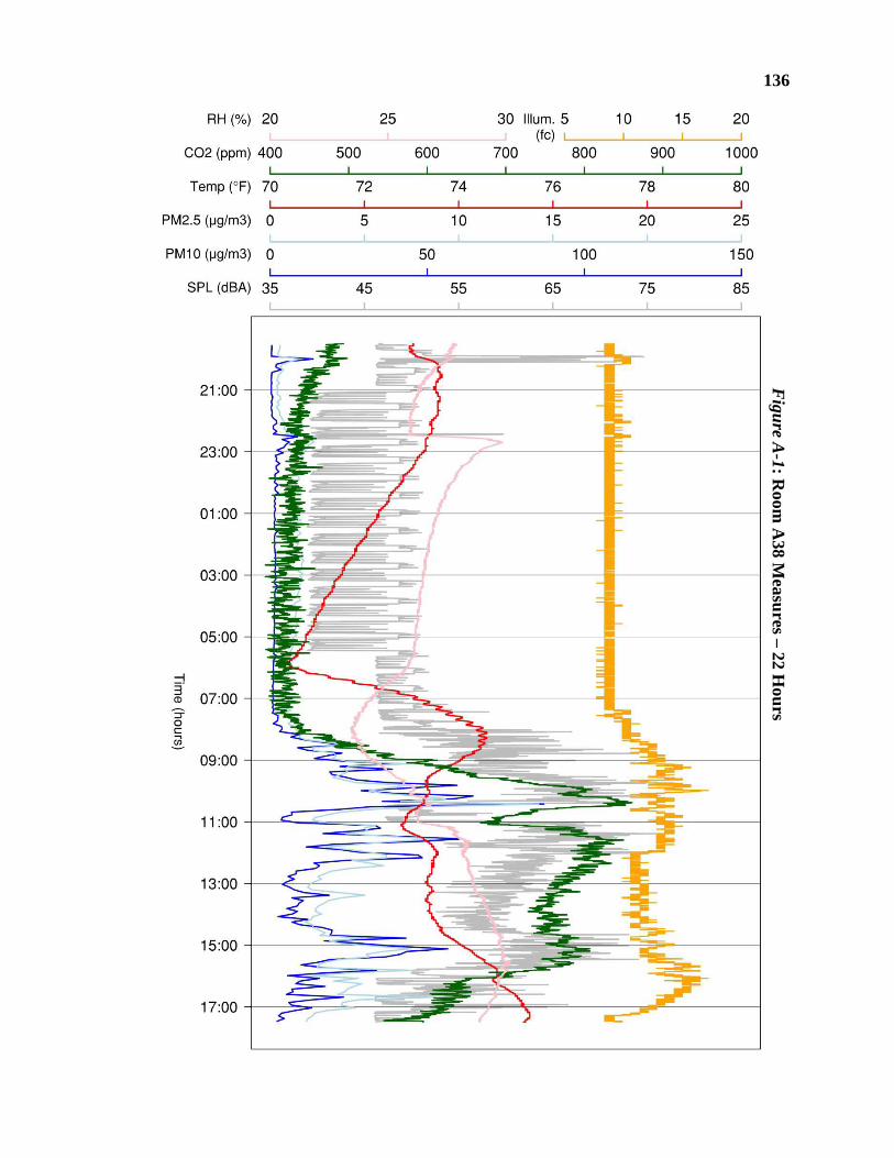
136
Figure A
-1: Room
A38 M
easures – 22 Hours

137
Figure A
-2: Room
B24 M
easures – 22 Hours

138
Figure A
-3: Room
A38 M
easures – 10 Hours

139
Figure A
-4: Room
A38 M
easures – 10 Hours

140
Figure A-5: Room A88 Particulate Matter Concentration 15-Minute TWA – Day 1
Figure A-6: Room A88 Particulate Matter Concentration 15-Minute TWA – Day 2
Figure A-7: Room A88 Particulate Matter Concentration 15-MinuteTWA – Day 3
0
500
1000
1500
2000
2500
7:3
3:5
6
8:0
5:1
4
8:3
6:3
2
9:0
7:5
0
9:3
9:0
8
10
:10
:26
10
:41
:44
11
:13
:02
11
:44
:20
12
:15
:38
12
:46
:56
13
:18
:14
13
:49
:32
14
:20
:50
14
:52
:08
15
:23
:26
15
:54
:44
16
:26
:02
16
:57
:20
µg/m
3
PM2.5
PM10
0
20
40
60
80
100
120
140
160
180
7:3
3:5
6
8:0
0:0
1
8:2
6:0
6
8:5
2:1
1
9:1
8:1
6
9:4
4:2
1
10
:10
:26
10
:36
:31
11
:02
:36
11
:28
:41
11
:54
:46
12
:20
:51
12
:46
:56
13
:13
:01
13
:39
:06
14
:05
:11
14
:31
:16
14
:57
:21
15
:23
:26
15
:49
:31
16
:15
:36
16
:41
:41
17
:07
:46
µg/m
3
PM2.5
PM10
0
200
400
600
800
1000
1200
1400
7:3
3:5
6
8:0
5:1
4
8:3
6:3
2
9:0
7:5
0
9:3
9:0
8
10
:10
:26
10
:41
:44
11
:13
:02
11
:44
:20
12
:15
:38
12
:46
:56
13
:18
:14
13
:49
:32
14
:20
:50
14
:52
:08
15
:23
:26
15
:54
:44
16
:26
:02
16
:57
:20
µg/m
3
PM2.5
PM10

Table A
-5: Exam
ple of Observational C
hecklist Data
Room
Area (ft2)
Color (no warm=-1; >=1 warm=1)
Ext Door
Plants (number)
Blinds (closed=-1; 1/2=0; open=1)
Hiding (places)
Flooring (fraction carpet)
Type (Infant=0; 1-2yrs=1; 2-3yrs=2; 3-5yrs=3)
Acoustic (separation, yes=1)
Switches
Orientation (clockwise degrees from north)
Glare (fraction w/ protection)
Lighting Power Density (LPD)
Illum Avg High
Illum Ratio
Tstat (no=-1; yes but covered=0; yes=1)
- 578
1 0
1 1
0 0.67
1 -1
3.5 0
1 2.52
72.5 1.96
1
- 574
1 0
1 1
2 0.50
2 -1
1.5 0
1 2.21
74.2 1.87
0
- 595
-1 0
1 -1
3 0.50
2 -1
1.5 0
1 2.22
71.2 2.62 0
- 563
1 0
1 0
1 0.60
0 -1
3.5 45
1 2.49
74.2 2.20
1
- 561
1 0
0 0
1 0.60
1 -1
3.5 135
0.75 2.46
76.4 2.
86 1
- 881
1 1
1 -1
1 0.15
3 -1
1.5 90
0.85 2.29
85.9 3.
02 1
- 850
-1 0
1 1
1 0.13
3 -1
1.5 135
0.6 2.31
97.3 2.
92 1
- 889
1 0
1 0
1 0.11
3 -1
1.5 -135
1 2.20
82.2 2.74
1
141

142
APPENDIX B - Outcome Variable Data
Figure B-1: Lead Teacher Survey Data by Classroom

143
Figure B-2: Assistant Teacher Survey Data by Classroom

144
Figure B-3: Teacher’s Aide Survey Data by Classroom

145
Figure B-4: Spearman’s Rank Correlation Significance for Survey Items

146
Table B-1: Lead Teacher Dataset Composite Raw Scores
clas
sroo
m
title
ten
ure
exp
eri
en
ce
tea
cha
ge
size
sat
vie
wsa
t
acc
sat2
the
rmsa
t
air
tot
ligh
tto
t
na
tura
ltot
furn
tot
cle
an
tot
org
sat
ieq
ove
rall
A18 1 2 4 4 4.0 5.0 4.7 4.1 5.7 5.5 5.5 4.5 4.2 3.9 5.0 A19 1 3 3 1 5.0 4.0 5.3 3.6 5.2 3.5 4.5 4.2 3.0 3.3 4.0 A28 2 3 2 1 5.0 5.3 4.0 1.7 3.2 5.5 6.0 4.2 3.3 4.0 5.0 A38 1 3 3 1 5.5 6.0 4.7 3.6 6.0 4.5 5.0 6.0 4.5 3.9 6.0 A46 1 3 1 1 5.0 4.7 5.0 3.4 3.0 3.5 5.0 4.8 4.2 4.0 5.0 A55 1 4 4 2 4.5 5.0 4.7 3.1 4.3 5.5 5.0 5.0 4.0 4.0 5.0 A64 1 4 3 1 5.5 5.3 4.0 3.4 5.2 5.0 5.0 5.8 4.7 3.3 5.0 A66 1 2 1 1 5.0 5.3 4.0 2.6 4.2 3.0 5.0 5.5 5.0 3.0 4.0 A88 1 3 3 1 4.5 3.3 5.0 2.9 5.7 5.5 3.5 5.2 3.5 3.3 4.0 A91 2 4 3 4 5.0 4.7 5.3 6.0 4.7 4.0 5.0 4.7 3.5 2.1 5.0 A94 1 4 4 4 5.0 5.3 4.7 3.1 4.5 5.5 5.5 3.5 3.2 3.3 5.0 B12 1 2 2 2 2.0 4.7 3.7 4.6 5.3 6.0 1.5 4.3 3.0 3.0 5.0 B17 1 3 2 1 4.0 2.7 2.0 2.7 3.2 2.5 2.0 1.5 2.8 3.0 5.0 B19 1 3 2 1 4.0 3.7 4.3 1.9 4.2 5.0 4.5 2.8 2.8 3.3 5.0 B25 1 2 4 2 5.5 5.3 4.3 2.3 5.5 5.5 6.0 5.0 4.3 3.9 6.0 B33 2 3 4 3 4.0 4.7 3.3 1.9 1.0 4.5 5.0 3.0 2.7 3.6 5.0 B54 2 3 4 4 3.0 5.0 5.0 2.7 4.8 4.0 3.0 4.2 2.3 3.3 4.0 B64 1 2 3 2 6.0 6.0 5.3 5.8 5.2 6.0 5.0 5.3 3.8 3.3 5.0 B66 1 2 3 1 2.5 4.3 4.0 3.6 5.3 6.0 5.0 3.5 2.2 3.4 4.0 B81 2 3 4 4 2.5 3.0 2.0 1.3 2.3 4.5 4.0 3.7 2.5 3.3 4.0 B89 1 4 4 4 5.0 3.7 3.7 4.3 3.8 5.5 5.0 4.5 3.0 3.7 4.0 B93 1 2 2 2 2.5 4.0 4.0 3.3 5.7 5.5 3.0 4.2 3.0 2.4 4.0 B97 1 2 3 1 6.0 5.0 5.3 3.3 5.2 6.0 4.0 4.8 4.0 4.0 6.0 µA 1.2 3.2 2.8 1.9 4.9 4.9 4.7 3.4 4.7 4.6 5.0 4.8 3.9 3.5 4.8 σA 0.4 0.8 1.1 1.4 0.4 0.7 0.5 1.1 1.0 1.0 0.6 0.8 0.7 0.6 0.6 µB 1.3 2.6 3.1 2.3 3.9 4.3 3.9 3.1 4.3 5.1 4.0 3.9 3.0 3.3 4.8 σB 0.5 0.7 0.9 1.2 1.4 1.0 1.1 1.3 1.5 1.1 1.4 1.1 0.7 0.4 0.8 µ 1.2 2.9 3.0 2.1 4.4 4.6 4.3 3.3 4.5 4.9 4.5 4.4 3.5 3.4 4.8 σ 0.4 0.8 1.0 1.3 1.2 0.9 0.9 1.2 1.2 1.0 1.2 1.0 0.8 0.5 0.7
p
µA≠µ
B
0.70
8
0.05
6
0.52
8
0.53
5
0.04
7*
0.11
8
0.05
0*
0.55
7
0.98
8
0.30
4
0.04
0*
0.02
6*
0.00
8**
0.67
0
0.81
4
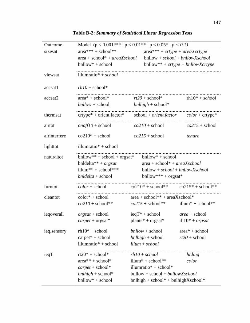
147
Table B-2: Summary of Statistical Linear Regression Tests
Outcome Model (p < 0.001*** p < 0.01** p < 0.05* p < 0.1) sizesat area*** + school** area*** + crtype + areaXcrtype area + school* + areaXschool bnllow + school + bnllowXschool bnllow* + school bnllow** + crtype + bnllowXcrtype
viewsat illumratio* + school
accsat1 rh10 + school*
accsat2 area* + school* rt20 + school* rh10* + school bnllow + school bnlhigh + school*
thermsat crtype* + orient.factor* school + orient.factor color + crtype*
airtot onoff10 + school co210 + school co215 + school
airinterfere co210* + school co215 + school tenure
lighttot illumratio* + school
naturaltot bnllow** + school + orgsat* bnllow* + school bnldelta** + orgsat area + school* + areaXschool illum** + school*** bnllow + school + bnllowXschool bnldelta + school bnllow*** + orgsat*
furntot color + school co210* + school** co215* + school**
cleantot color* + school area + school** + areaXschool* co210 + school** co215 + school** illum* + school**
ieqoverall orgsat + school ieqT* + school area + school carpet + orgsat* plants* + orgsat* rh10* + orgsat
ieq.sensory rh10* + school bnllow + school area* + school carpet* + school bnlhigh + school rt20 + school illumratio* + school illum + school
ieqT rt20* + school* rh10 + school hiding area** + school* illum* + school** color carpet + school* illumratio* + school* bnlhigh + school* bnllow + school + bnllowXschool bnllow* + school bnlhigh + school* + bnlhighXschool*
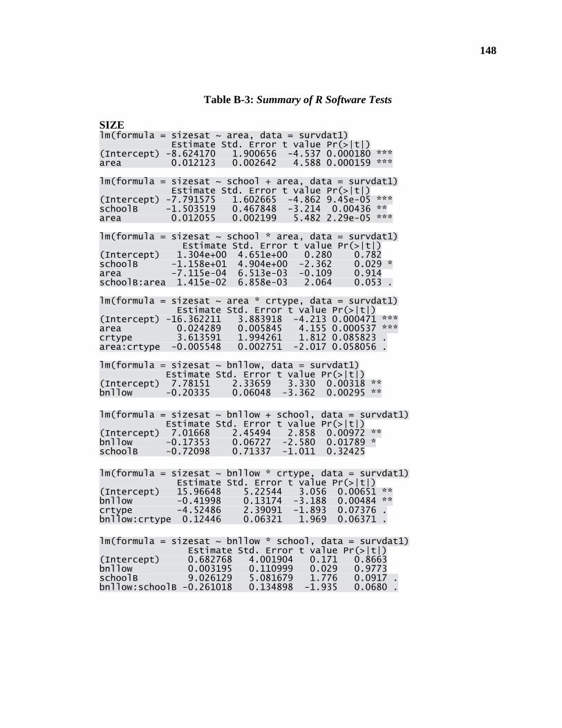
148
Table B-3: Summary of R Software Tests
SIZE lm(formula = sizesat ~ area, data = survdat1) Estimate Std. Error t value Pr(>|t|) (Intercept) -8.624170 1.900656 -4.537 0.000180 *** area 0.012123 0.002642 4.588 0.000159 *** lm(formula = sizesat ~ school + area, data = survdat1) Estimate Std. Error t value Pr(>|t|) (Intercept) -7.791575 1.602665 -4.862 9.45e-05 *** schoolB -1.503519 0.467848 -3.214 0.00436 ** area 0.012055 0.002199 5.482 2.29e-05 *** lm(formula = sizesat ~ school * area, data = survdat1) Estimate Std. Error t value Pr(>|t|) (Intercept) 1.304e+00 4.651e+00 0.280 0.782 schoolB -1.158e+01 4.904e+00 -2.362 0.029 * area -7.115e-04 6.513e-03 -0.109 0.914 schoolB:area 1.415e-02 6.858e-03 2.064 0.053 . lm(formula = sizesat ~ area * crtype, data = survdat1) Estimate Std. Error t value Pr(>|t|) (Intercept) -16.362211 3.883918 -4.213 0.000471 *** area 0.024289 0.005845 4.155 0.000537 *** crtype 3.613591 1.994261 1.812 0.085823 . area:crtype -0.005548 0.002751 -2.017 0.058056 . lm(formula = sizesat ~ bnllow, data = survdat1) Estimate Std. Error t value Pr(>|t|) (Intercept) 7.78151 2.33659 3.330 0.00318 ** bnllow -0.20335 0.06048 -3.362 0.00295 **
lm(formula = sizesat ~ bnllow + school, data = survdat1) Estimate Std. Error t value Pr(>|t|) (Intercept) 7.01668 2.45494 2.858 0.00972 ** bnllow -0.17353 0.06727 -2.580 0.01789 * schoolB -0.72098 0.71337 -1.011 0.32425
lm(formula = sizesat ~ bnllow * crtype, data = survdat1) Estimate Std. Error t value Pr(>|t|) (Intercept) 15.96648 5.22544 3.056 0.00651 ** bnllow -0.41998 0.13174 -3.188 0.00484 ** crtype -4.52486 2.39091 -1.893 0.07376 . bnllow:crtype 0.12446 0.06321 1.969 0.06371 .
lm(formula = sizesat ~ bnllow * school, data = survdat1) Estimate Std. Error t value Pr(>|t|) (Intercept) 0.682768 4.001904 0.171 0.8663 bnllow 0.003195 0.110999 0.029 0.9773 schoolB 9.026129 5.081679 1.776 0.0917 . bnllow:schoolB -0.261018 0.134898 -1.935 0.0680 .

149
Table B-3: Summary of R Software Tests, continued
VIEWS lm(formula = viewsat ~ illumratio, data = survdat1) Estimate Std. Error t value Pr(>|t|) (Intercept) -6.532 3.183 -2.052 0.0528 . illumratio 2.618 1.262 2.075 0.0505 . lm(formula = viewsat ~ illumratio + school, data = survdat1) Estimate Std. Error t value Pr(>|t|) (Intercept) -5.8990 3.0243 -1.951 0.0653 . illumratio 2.7158 1.1927 2.277 0.0339 * schoolB -1.6784 0.8908 -1.884 0.0742 . lm(formula = ieqoverall ~ viewsat, data = survdat1) Estimate Std. Error t value Pr(>|t|) (Intercept) -3.088e-17 1.821e-01 0.000 1.0000 viewsat 2.155e-01 7.688e-02 2.802 0.0107 *
ACOUSTICS lm(formula = rt20 ~ area, data = survdat1) Estimate Std. Error t value Pr(>|t|) (Intercept) 3.060e-01 4.203e-02 7.280 3.61e-07 *** area 1.699e-04 5.843e-05 2.908 0.00842 **
lm(formula = accsat2 ~ area + school, data = survdat1) Estimate Std. Error t value Pr(>|t|) (Intercept) -6.089350 2.724332 -2.235 0.0370 * area 0.009922 0.003738 2.654 0.0152 * schoolB -1.857325 0.795284 -2.335 0.0301 * lm(formula = accsat2 ~ rt20 + school, data = survdat1) Estimate Std. Error t value Pr(>|t|) (Intercept) -8.7701 5.5360 -1.584 0.1288 rt20 23.3229 13.1594 1.772 0.0916 . schoolB -2.2701 0.8878 -2.557 0.0188 * lm(formula = accsat2 ~ bnllow + school, data = survdat1) Estimate Std. Error t value Pr(>|t|) (Intercept) 7.09183 3.25630 2.178 0.0416 * bnllow -0.17054 0.08922 -1.911 0.0704 . schoolB -1.08435 0.94623 -1.146 0.2653
lm(formula = accsat2 ~ bnlhigh + school, data = survdat1) Estimate Std. Error t value Pr(>|t|) (Intercept) 10.6636 4.9595 2.150 0.0440 * bnlhigh -0.2004 0.1019 -1.968 0.0631 . schoolB -2.0680 0.8520 -2.427 0.0248 * lm(formula = accsat2 ~ rh10 + school, data = survdat1) Estimate Std. Error t value Pr(>|t|) (Intercept) -3.90872 1.89867 -2.059 0.0528 . rh10 0.21941 0.08126 2.700 0.0138 * schoolB -1.63151 0.79691 -2.047 0.0540 . lm(formula = accsat1 ~ rh10 + school, data = survdat1) Estimate Std. Error t value Pr(>|t|) (Intercept) -4.0154 2.9216 -1.374 0.1845 rh10 0.2598 0.1250 2.077 0.0509 . schoolB -3.1055 1.2262 -2.533 0.0198 *

150
Table B-3: Summary of R Software Tests, continued
lm(formula = stcsat ~ laeq10 + school, data = survdat1) Estimate Std. Error t value Pr(>|t|) (Intercept) -13.45338 5.08362 -2.646 0.01549 * laeq10 0.21448 0.07907 2.713 0.01340 * schoolB -1.29382 0.43546 -2.971 0.00755 **
TEMPERATURE lm(formula = thermsat ~ crtype, data = survdat1) Estimate Std. Error t value Pr(>|t|) (Intercept) -2.2041 1.1640 -1.894 0.0721 . crtype 1.3701 0.6055 2.263 0.0344 * lm(formula = thermsat ~ crtype + school, data = survdat1) Estimate Std. Error t value Pr(>|t|) (Intercept) -1.7880 1.3747 -1.301 0.2082 crtype 1.3609 0.6152 2.212 0.0388 * schoolB -0.7692 1.2963 -0.593 0.5596 lm(formula = thermsat ~ orient.factor + crtype, data = survdat1) Estimate Std. Error t value Pr(>|t|) (Intercept) -1.0072 0.3570 -2.821 0.0105 * orient.factor1 0.7843 0.3546 2.212 0.0388 * crtype 0.4141 0.1670 2.480 0.0222 *
lm(formula = thermsat ~ orient.factor + school, data = survdat1) Estimate Std. Error t value Pr(>|t|) (Intercept) -0.1695 0.3198 -0.530 0.602 orient.factor1 0.8285 0.4009 2.067 0.052 . schoolB -0.3656 0.3979 -0.919 0.369
lm(formula = thermsat ~ crtype + color, data = survdat1) Estimate Std. Error t value Pr(>|t|) (Intercept) -0.3686 0.3614 -1.020 0.3199 crtype 0.4585 0.1726 2.657 0.0151 * color1 -0.7072 0.3636 -1.945 0.0659 .
AIR QUALITY lm(formula = airinterfere ~ tenure, data = survdat1) Estimate Std. Error t value Pr(>|t|) (Intercept) 1.5138 0.7804 1.940 0.0666 . tenure -0.5286 0.2635 -2.006 0.0585 .
lm(formula = airinterfere ~ co210 + school, data = survdat1) Estimate Std. Error t value Pr(>|t|) (Intercept) 7.290805 3.012798 2.420 0.0257 * co210 -0.010264 0.004096 -2.506 0.0215 * schoolB 0.049147 0.411647 0.119 0.9062
lm(formula = airtot ~ co210 + school, data = survdat1) Estimate Std. Error t value Pr(>|t|) (Intercept) 14.44811 7.44612 1.940 0.0673 . co210 -0.01948 0.01012 -1.924 0.0694 . schoolB -0.76311 1.01739 -0.750 0.4624

151
Table B-3: Summary of R Software Tests, continued
lm(formula = airtot ~ co215 + school, data = survdat1) Estimate Std. Error t value Pr(>|t|) (Intercept) 4.234131 2.337779 1.811 0.0860 . co215 -0.004742 0.002596 -1.827 0.0835 . schoolB -0.370674 0.462110 -0.802 0.4324
LIGHTING lm(formula = lighttot ~ illumratio + school, data = survdat1) Estimate Std. Error t value Pr(>|t|) (Intercept) -4.5780 1.9253 -2.378 0.0275 * illumratio 1.7105 0.7593 2.253 0.0357 * schoolB 0.5964 0.5671 1.052 0.3055 lm(formula = naturaltot ~ area * school, data = survdat1) Estimate Std. Error t value Pr(>|t|) (Intercept) 5.854017 5.577195 1.050 0.3071 area -0.007198 0.007810 -0.922 0.3683 schoolB -12.711617 5.880441 -2.162 0.0436 * area:schoolB 0.015915 0.008224 1.935 0.0680 . lm(formula = naturaltot ~ bnllow + school, data = survdat1) Estimate Std. Error t value Pr(>|t|) (Intercept) 6.46156 2.12290 3.044 0.00641 ** bnllow -0.16004 0.05817 -2.751 0.01231 * schoolB -0.64613 0.61688 -1.047 0.30740 lm(formula = naturaltot ~ bnllow * school, data = survdat1) Estimate Std. Error t value Pr(>|t|) (Intercept) 0.820939 3.439917 0.239 0.8139 bnllow -0.002663 0.095411 -0.028 0.9780 schoolB 8.034080 4.368060 1.839 0.0816 . bnllow:schoolB -0.232447 0.115954 -2.005 0.0595 . lm(formula = naturaltot ~ orgsat + bnllow, data = survdat1) Estimate Std. Error t value Pr(>|t|) (Intercept) 7.18778 1.75019 4.107 0.000548 *** orgsat 0.14515 0.05103 2.845 0.010017 * bnllow -0.18783 0.04530 -4.146 0.000500 *** lm(formula = naturaltot ~ orgsat + bnllow + school, data = survdat1) Estimate Std. Error t value Pr(>|t|) (Intercept) 4.04792 1.12278 3.605 0.00189 ** orgsat 0.40894 0.15052 2.717 0.01368 * bnllow -0.10175 0.03079 -3.305 0.00372 ** schoolB -0.29558 0.32791 -0.901 0.37866 lm(formula = naturaltot ~ bnldelta + orgsat, data = survdat1) (Intercept) -1.15290 0.41113 -2.804 0.01095 * bnldelta 0.12068 0.03947 3.058 0.00621 ** orgsat 0.34907 0.16917 2.063 0.05229 . lm(formula = naturaltot ~ bnldelta + school, data = survdat1) Estimate Std. Error t value Pr(>|t|) (Intercept) -1.01086 0.76432 -1.323 0.2009 bnldelta 0.11632 0.05761 2.019 0.0571 . schoolB -0.19238 0.48349 -0.398 0.6949

152
Table B-3: Summary of R Software Tests, continued
lm(formula = naturaltot ~ bnldelta + orgsat + school, data = survdat1) Estimate Std. Error t value Pr(>|t|) (Intercept) -0.91304 0.71326 -1.280 0.2159 bnldelta 0.10580 0.05389 1.963 0.0644 . orgsat 0.34866 0.17278 2.018 0.0579 . schoolB -0.18727 0.45016 -0.416 0.6821 lm(formula = naturaltot ~ illum + school, data = survdat1) Estimate Std. Error t value Pr(>|t|) (Intercept) -4.23798 1.45157 -2.920 0.00847 ** illum 0.09386 0.02875 3.264 0.00388 ** schoolB -3.73971 0.94274 -3.967 0.00076 ***
FURNISHINGS lm(formula = furntot ~ co210 + school, data = survdat1) Estimate Std. Error t value Pr(>|t|) (Intercept) 33.37299 13.24796 2.519 0.02038 * co210 -0.04247 0.01801 -2.358 0.02866 * schoolB -6.10945 1.80270 -3.389 0.00291 ** lm(formula = furntot ~ co215 + school, data = survdat1) Estimate Std. Error t value Pr(>|t|) (Intercept) 24.24878 9.40070 2.579 0.0179 * co215 -0.02461 0.01044 -2.358 0.0287 * schoolB -6.36475 1.85078 -3.439 0.0026 ** lm(formula = furntot ~ color + crtype, data = survdat1) Estimate Std. Error t value Pr(>|t|) (Intercept) 0.44390 0.37400 1.187 0.2492 color1 -1.03852 0.37626 -2.760 0.0121 * crtype 0.06088 0.17858 0.341 0.7367 lm(formula = furntot ~ color + school, data = survdat1) Estimate Std. Error t value Pr(>|t|) (Intercept) 0.6808 0.2815 2.419 0.0252 * color1 -0.7609 0.4074 -1.868 0.0765 . schoolB -0.5439 0.4074 -1.335 0.1968 lm(formula = furntot ~ color, data = survdat1) Estimate Std. Error t value Pr(>|t|) (Intercept) 0.5325 0.2634 2.022 0.0561 . color1 -1.0205 0.3646 -2.799 0.0108 *
CLEANING lm(formula = cleantot ~ color + school, data = survdat1) Estimate Std. Error t value Pr(>|t|) (Intercept) 3.180 0.999 3.183 0.00467 ** color1 -3.633 1.446 -2.512 0.02068 * schoolB -2.462 1.446 -1.702 0.10419 lm(formula = cleantot ~ illum + school, data = survdat1) Estimate Std. Error t value Pr(>|t|) (Intercept) -12.4635 5.7405 -2.171 0.04213 * illum 0.2940 0.1137 2.585 0.01768 * schoolB -13.2654 3.7283 -3.558 0.00197 **

153
Table B-3: Summary of R Software Tests, continued
lm(formula = cleantot ~ rt20 + school, data = survdat1) Estimate Std. Error t value Pr(>|t|) (Intercept) -15.817 8.466 -1.868 0.07643 . rt20 43.074 20.124 2.140 0.04483 * schoolB -4.921 1.358 -3.624 0.00169 ** lm(formula = cleantot ~ co210 + school, data = survdat1) Estimate Std. Error t value Pr(>|t|) (Intercept) 5.992934 2.719206 2.204 0.03941 * co210 -0.007425 0.003696 -2.009 0.05827 . schoolB -1.371766 0.370013 -3.707 0.00139 ** lm(formula = cleantot ~ co215 + school, data = survdat1) Estimate Std. Error t value Pr(>|t|) (Intercept) 4.510353 1.917939 2.352 0.02905 * co215 -0.004429 0.002129 -2.080 0.05061 . schoolB -1.426843 0.377597 -3.779 0.00118 ** lm(formula = cleantot ~ area * school, data = survdat1) Estimate Std. Error t value Pr(>|t|) (Intercept) 5.800420 3.129442 1.854 0.07940 . area -0.007365 0.004382 -1.681 0.10920 schoolB -9.550543 3.299597 -2.894 0.00929 ** area:schoolB 0.011931 0.004614 2.586 0.01814 *
IEQ OVERALL lm(formula = ieqoverall ~ orgsat + school, data = survdat1) Estimate Std. Error t value Pr(>|t|) (Intercept) 0.01698 0.29345 0.058 0.9544 orgsat 0.37600 0.20794 1.808 0.0856 . schoolB -0.03254 0.40712 -0.080 0.9371 lm(formula = ieqoverall ~ orgsat + plants, data = survdat1) Estimate Std. Error t value Pr(>|t|) (Intercept) -0.42438 0.27273 -1.556 0.1354 orgsat 0.09933 0.04021 2.470 0.0226 * plants 0.39043 0.18581 2.101 0.0485 * lm(formula = ieqoverall ~ orgsat + carpet, data = survdat1) Estimate Std. Error t value Pr(>|t|) (Intercept) 0.58207 0.36295 1.604 0.1245 orgsat 0.08322 0.03980 2.091 0.0495 * carpet -1.54665 0.82685 -1.871 0.0761 . lm(formula = ieqoverall ~ rh10 + orgsat, data = survdat1) Estimate Std. Error t value Pr(>|t|) (Intercept) -1.75737 0.83366 -2.108 0.0478 * rh10 0.08101 0.03750 2.160 0.0431 * orgsat 0.06834 0.03905 1.750 0.0954 . lm(formula = ieqoverall ~ ieqT + school, data = survdat1) Estimate Std. Error t value Pr(>|t|) (Intercept) -0.1592 0.2943 -0.541 0.5948 ieqT 0.5452 0.2220 2.456 0.0238 * schoolB 0.2889 0.4337 0.666 0.5133 lm(formula = ieq.sensory ~ area + school, data = survdat1) Estimate Std. Error t value Pr(>|t|) (Intercept) -2.950265 1.281645 -2.302 0.0328 * area 0.004419 0.001759 2.512 0.0212 * schoolB -0.367075 0.380520 -0.965 0.3468

154
Table B-3: Summary of R Software Tests, continued
lm(formula = ieq.sensory ~ illumratio + school, data = survdat1) Estimate Std. Error t value Pr(>|t|) (Intercept) -3.1256 1.2557 -2.489 0.0222 * illumratio 1.3413 0.4955 2.707 0.0140 * schoolB -0.4061 0.3730 -1.089 0.2899 lm(formula = ieq.sensory ~ illum + school, data = survdat1) Estimate Std. Error t value Pr(>|t|) (Intercept) -2.94543 1.83337 -1.607 0.1246 illum 0.06307 0.03633 1.736 0.0987 . schoolB -2.32109 1.18172 -1.964 0.0643 . lm(formula = ieq.sensory ~ carpet + school, data = survdat1) Estimate Std. Error t value Pr(>|t|) (Intercept) 0.9580 0.4585 2.090 0.0503 . carpet -1.8502 0.8839 -2.093 0.0500 * schoolB -0.4816 0.3979 -1.211 0.2409 lm(formula = ieq.sensory ~ rh10 + school, data = survdat1) Estimate Std. Error t value Pr(>|t|) (Intercept) -1.80325 0.91209 -1.977 0.0627 . rh10 0.08982 0.03904 2.301 0.0329 * schoolB -0.28800 0.39105 -0.736 0.4704 lm(formula = ieq.sensory ~ bnllow + school, data = survdat1) Estimate Std. Error t value Pr(>|t|) (Intercept) 3.23600 1.63168 1.983 0.062 . bnllow -0.08477 0.04483 -1.891 0.074 . schoolB 0.06358 0.47027 0.135 0.894 lm(formula = ieq.sensory ~ bnlhigh + school, data = survdat1) Estimate Std. Error t value Pr(>|t|) (Intercept) 5.07552 2.42678 2.091 0.0502 . bnlhigh -0.10095 0.04989 -2.024 0.0573 . schoolB -0.43198 0.39859 -1.084 0.2920 lm(formula = ieq.sensory ~ rt20 + school, data = survdat1) Estimate Std. Error t value Pr(>|t|) (Intercept) -4.4394 2.6068 -1.703 0.1049 rt20 11.0930 6.1980 1.790 0.0894 . schoolB -0.5536 0.4156 -1.332 0.1986 lm(formula = ieqT ~ area + school, data = survdat1) Estimate Std. Error t value Pr(>|t|) (Intercept) -3.105370 1.116866 -2.780 0.01192 * area 0.004905 0.001533 3.200 0.00471 ** schoolB -0.746680 0.331597 -2.252 0.03636 * lm(formula = ieqT ~ illumratio + school, data = survdat1) Estimate Std. Error t value Pr(>|t|) (Intercept) -2.6213 1.1907 -2.202 0.0403 * illumratio 1.2151 0.4699 2.586 0.0181 * schoolB -0.7878 0.3537 -2.228 0.0382 * lm(formula = ieqT ~ illum + school, data = survdat1) Estimate Std. Error t value Pr(>|t|) (Intercept) -3.78687 1.57334 -2.407 0.02642 * illum 0.08379 0.03117 2.688 0.01457 * schoolB -3.33652 1.01412 -3.290 0.00385 **

155
Table B-3: Summary of R Software Tests, continued
lm(formula = ieqT ~ rt20 + school, data = survdat1) Estimate Std. Error t value Pr(>|t|) (Intercept) -5.0169 2.3259 -2.157 0.0440 * rt20 12.9323 5.5300 2.339 0.0304 * schoolB -0.9625 0.3708 -2.596 0.0177 * lm(formula = ieqT ~ color + crtype, data = survdat1) Estimate Std. Error t value Pr(>|t|) (Intercept) 0.00131 0.38182 0.003 0.9973 color1 -0.90520 0.39189 -2.310 0.0323 * crtype 0.27579 0.18348 1.503 0.1493 lm(formula = ieqT ~ carpet + school, data = survdat1) Estimate Std. Error t value Pr(>|t|) (Intercept) 1.0713 0.4335 2.471 0.0231 * carpet -1.6600 0.8357 -1.986 0.0616 . schoolB -0.8555 0.3762 -2.274 0.0347 * lm(formula = ieqT ~ rh10 + school, data = survdat1) Estimate Std. Error t value Pr(>|t|) (Intercept) -1.13237 0.89395 -1.267 0.2206 rh10 0.06829 0.03826 1.785 0.0903 . schoolB -0.69652 0.38327 -1.817 0.0850 . lm(formula = ieqT ~ bnllow + school, data = survdat1) Estimate Std. Error t value Pr(>|t|) (Intercept) 3.53717 1.49577 2.365 0.0288 * bnllow -0.08783 0.04109 -2.137 0.0458 * schoolB -0.30257 0.43110 -0.702 0.4913 lm(formula = ieqT ~ bnlhigh + school, data = survdat1) Estimate Std. Error t value Pr(>|t|) (Intercept) 4.57847 2.31168 1.981 0.0623 . bnlhigh -0.08671 0.04752 -1.825 0.0838 . schoolB -0.80959 0.37968 -2.132 0.0463 * lm(formula = ieqT ~ bnlhigh * school, data = survdat1) Estimate Std. Error t value Pr(>|t|) (Intercept) 0.91059 2.58780 0.352 0.7290 bnlhigh -0.01079 0.05333 -0.202 0.8419 schoolB 9.30145 4.28132 2.173 0.0434 * bnlhigh:schoolB -0.21027 0.08875 -2.369 0.0292 * lm(formula = ieqT ~ bnllow * school, data = survdat1) Estimate Std. Error t value Pr(>|t|) (Intercept) 0.279978 2.269096 0.123 0.9032 bnllow 0.003047 0.062937 0.048 0.9619 schoolB 5.245236 3.054251 1.717 0.1031 bnllow:schoolB -0.146400 0.079881 -1.833 0.0834 .

156
APPENDIX C - Participant Survey

157

158

159

160

161
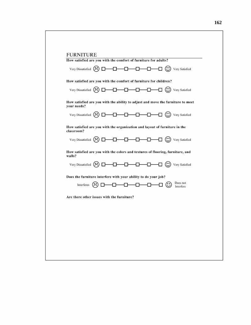
162

163

164