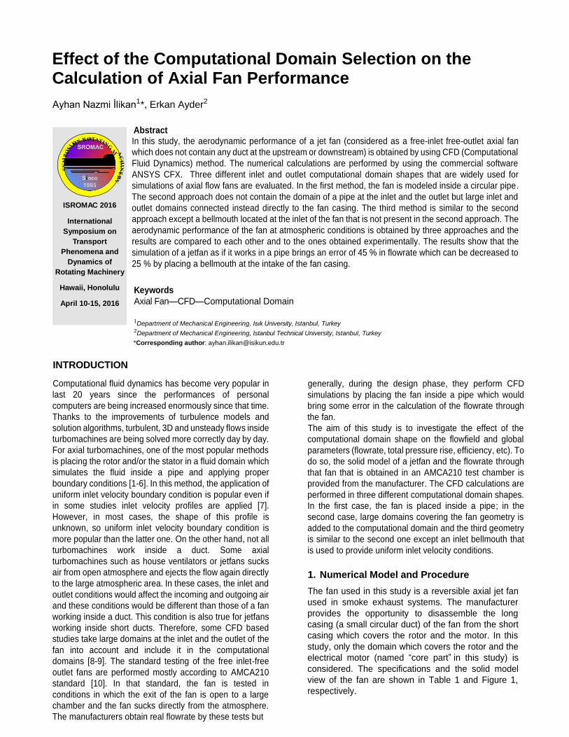
Effect of the Computational Domain Selection on the Calculation of Axial Fan Performance

Ayhan Nazmi İlikan1*, Erkan Ayder2

ISROMAC 2016

International

Symposium on

Transport

Phenomena and

Dynamics of

Rotating Machinery

Hawaii, Honolulu

April 10-15, 2016

Abstract In this study, the aerodynamic performance of a jet fan (considered as a free-inlet free-outlet axial fan

which does not contain any duct at the upstream or downstream) is obtained by using CFD (Computational

Fluid Dynamics) method. The numerical calculations are performed by using the commercial software

ANSYS CFX. Three different inlet and outlet computational domain shapes that are widely used for

simulations of axial flow fans are evaluated. In the first method, the fan is modeled inside a circular pipe.

The second approach does not contain the domain of a pipe at the inlet and the outlet but large inlet and

outlet domains connected instead directly to the fan casing. The third method is similar to the second

approach except a bellmouth located at the inlet of the fan that is not present in the second approach. The

aerodynamic performance of the fan at atmospheric conditions is obtained by three approaches and the

results are compared to each other and to the ones obtained experimentally. The results show that the

simulation of a jetfan as if it works in a pipe brings an error of 45 % in flowrate which can be decreased to

25 % by placing a bellmouth at the intake of the fan casing.

Keywords

Axial Fan—CFD—Computational Domain

1Department of Mechanical Engineering, Isık University, Istanbul, Turkey 2Department of Mechanical Engineering, Istanbul Technical University, Istanbul, Turkey

*Corresponding author: ayhan.ilikan@isikun.edu.tr

INTRODUCTION

Computational fluid dynamics has become very popular in

last 20 years since the performances of personal

computers are being increased enormously since that time.

Thanks to the improvements of turbulence models and

solution algorithms, turbulent, 3D and unsteady flows inside

turbomachines are being solved more correctly day by day.

For axial turbomachines, one of the most popular methods

is placing the rotor and/or the stator in a fluid domain which

simulates the fluid inside a pipe and applying proper

boundary conditions [1-6]. In this method, the application of

uniform inlet velocity boundary condition is popular even if

in some studies inlet velocity profiles are applied [7].

However, in most cases, the shape of this profile is

unknown, so uniform inlet velocity boundary condition is

more popular than the latter one. On the other hand, not all

turbomachines work inside a duct. Some axial

turbomachines such as house ventilators or jetfans sucks

air from open atmosphere and ejects the flow again directly

to the large atmospheric area. In these cases, the inlet and

outlet conditions would affect the incoming and outgoing air

and these conditions would be different than those of a fan

working inside a duct. This condition is also true for jetfans

working inside short ducts. Therefore, some CFD based

studies take large domains at the inlet and the outlet of the

fan into account and include it in the computational

domains [8-9]. The standard testing of the free inlet-free

outlet fans are performed mostly according to AMCA210

standard [10]. In that standard, the fan is tested in

conditions in which the exit of the fan is open to a large

chamber and the fan sucks directly from the atmosphere.

The manufacturers obtain real flowrate by these tests but

generally, during the design phase, they perform CFD

simulations by placing the fan inside a pipe which would

bring some error in the calculation of the flowrate through

the fan.

The aim of this study is to investigate the effect of the

computational domain shape on the flowfield and global

parameters (flowrate, total pressure rise, efficiency, etc). To

do so, the solid model of a jetfan and the flowrate through

that fan that is obtained in an AMCA210 test chamber is

provided from the manufacturer. The CFD calculations are

performed in three different computational domain shapes.

In the first case, the fan is placed inside a pipe; in the

second case, large domains covering the fan geometry is

added to the computational domain and the third geometry

is similar to the second one except an inlet bellmouth that

is used to provide uniform inlet velocity conditions.

1. Numerical Model and Procedure

The fan used in this study is a reversible axial jet fan

used in smoke exhaust systems. The manufacturer

provides the opportunity to disassemble the long

casing (a small circular duct) of the fan from the short

casing which covers the rotor and the motor. In this

study, only the domain which covers the rotor and the

electrical motor (named “core part” in this study) is

considered. The specifications and the solid model

view of the fan are shown in Table 1 and Figure 1,

respectively.

Effect of the Computational Domain Selection on the Calculation of Axial Fan Performance — 2

Table1.Specifications of the Jet Fan

Dshroud [mm] 310

Dhub/Dtip [ - ] 0.3

Tip clearance [mm] 3

Number of blades [ - ] 6

Rotational speed [rpm] 2930

Thrust (Catalogue) [N] 14

Φ (Catalogue) [ - ] 0.266

Figure1. Jet Fan

1.1 Computational Domain and Grid Generation

The first computational domain (namely 1st case in this

study) consists of the core part of the fan and the axial

extensions that represent pipes at the upstream and the

downstream of the fan. The axial lengths of these pipes

are chosen as 1D where D refers to the tip diameter of the

fan (Figure 2).

(a)

(b)

Figure2.The computational grid composed of the fan and

the pipes by (a) internal (b) external view (1st case)

The second computational domain (namely 2nd case in

this study) consists of large domains that cover the core

part of the fan. These domains are thought to represent

the physics of the flow at the opening regions of the fan

to the atmosphere, more realistically. The axial lengths

and the diameters of these large domains are chosen this

time as 2.5D and 4D, respectively (Figure 3).

Figure3.The computational grid composed of the large

domains (2nd and 3rd cases)

The third approach (namely 3rd case in this study) is

similar to the second case. The only difference is the

presence of a bellmouth shaped geometry at the inlet of

the casing of the fan. The bell mouth region in the third

approach and the sharp entrance region in the second

approach are shown in a closer view in Figure 4.

(a)

(b)

Figure4.The comparisons of the entrance regions of the

second (a) and third (b) approaches

In all the calculations, only one rotor blade and one motor

support plate passages are modeled since the flow is

axisymmetric in the direction of the rotation. These

support plates are kept in the numerical study for

comparison with experimental results and should not be

confused with stator blades. Since they are not designed

as stator blades which follow the absolute flow at the exit

of the rotor blades and orient it to the axial direction in

order to convert excess kinetic energy due to swirl in to

the pressure head. As the number of the rotor and support

plates are different (6 rotor blades and 4 motor support

plates), the extents of the inlet and rotor domains in theta

direction cover sectors of 60°, while the motor support

plates and the outlet domains, 90°. The difference of the

thickness of the sectors is carried out by the “stage”

Effect of the Computational Domain Selection on the Calculation of Axial Fan Performance — 3

interface that will be explained in the further sections.

The computational grid is generated by ANSYS Mesh.

Hexahedral and tetrahedral elements are both used

where applicable. In the core part of the fan, tetrahedral

elements are chosen due to the complexity of the

geometry. The generated mesh for this part of the model

is kept the same in all the three computational domain

configurations. The rest of the domains (inlet and outlet

pipes for the first case and large domains for the second

and third cases) are meshed by hexahedral elements to

decrease the computational time. Inflation layers are

added to all solid surfaces (hub, shroud and the blades of

the rotor and the electrical motor; pipe walls) and kept the

maximum y+ values of these surfaces around 1 to capture

the flow physics inside the boundary layers. A section that

shows the mesh around the blade and a list of the number

of elements related to different domains are shown in

Figure 5 and Table 2, respectively.

Table 2.Mesh information

Element type # of elements

Rotor Tetrahedral 2469224

Electrical Motor Support

Plates

Tetrahedral 2750409

Inlet & Outlet pipes

(1st case)

Hexahedral 955410

Inlet & Outlet

large domains (2nd case)

Hexahedral 2022140

Inlet & Outlet

large domains (3rd case)

Hexahedral 2199370

1st case (total) Both 6175043

2nd case (total) Both 7241773

3rd case (total) Both 7419003

Figure5.The mesh around the rotor blade

1.2 The Numerical Algorithm

The flow is modeled as 3D, incompressible, steady and

fully turbulent. The finite volume solver ANSYS CFX [11]

is used for the calculations of the flowfield. A second order

accurate scheme is chosen for the convection equations.

k-ω SST turbulent model [12] is used for the closure

problem during RANS calculations since it is known as

powerful to predict the flow separation [13]. y+ values are

kept around 1 near the solid walls to benefit from the near

wall treatment for low-Re number computation of the

turbulence model. Air at 25°C is used in all the

calculations as the working fluid.

1.3 Boundary Conditions

The frame change at the interface between the rotational

domain and the stationary domain is chosen as the

“stage” model which performs a circumferential averaging

of the fluxes through bands on the interface. Since the

angle of the section of the rotor and the support are not

the same (60° and 90°, respectively), an intersection

algorithm provided by the “stage” option provided by the

code, called “specified pitch angles” is used at this

interface. This option provides to specify the pitch angles

on two sides of the domain interface. The pitch change

adjustment is performed by applying average values

obtained from the upstream side of the interface to the

downstream side. The rotational speed of the fan is

imposed to the rotational domain and the rest of the

domains are kept stationary. The solid surfaces which

belong to the stationary and rotational domains are

modeled as stationary and rotating walls, respectively.

Counter rotating wall boundary condition with the same

magnitude but the opposite direction to the rotation of the

blades is imposed to the shroud surface of the rotating

domain to make this surface fixed in stationary frame. In

the first case, the “uniform inlet total pressure” boundary

condition is imposed to the inlet of the pipe. The total

pressure value in this surface is set as zero since the fan

in consideration works in atmospheric conditions. The

“opening pressure” boundary condition is imposed to the

outlet boundary of the pipe of this case and also to the

external surfaces of the outlet large domains of the

second and third cases. The reason of the usage of the

opening type boundary condition instead of outlet static

pressure option is about the direction of flow. Static

pressure option in CFX does not allow reverse flow at

outlet boundaries. If the code calculates reverse flow at

these boundaries, it imposes artificial walls which are not

physically true. This problem is solved by opening

pressure boundary condition which allows bidirectional

flow. During the calculations, this opening pressure is

kept at atmospheric conditions (0 Pa gage pressure).

The conditions that define turbulence properties at the

“inlet” and “outlet” surfaces are set as “zero gradient” that

is recommended by the code when opening boundary

condition is used in one of the boundaries. Since the flow

is modeled as periodic, periodic boundary conditions are

imposed to side surfaces.

2. RESULTS AND DISCUSSION

In this section, the results obtained from the calculations

will be presented by means of charts, contours and tables

obtained at the inlet and outlet of the fan, as well as the

passage domain.

Effect of the Computational Domain Selection on the Calculation of Axial Fan Performance — 4

Table 3 shows flow coefficient Φ, total pressure rise

coefficient Ψ, thrust T, total efficiency ηt values obtained

from the simulations realized under atmospheric

conditions. The flow coefficient and thrust values are

compared to the experimental ones that are already

shown in Table 1, obtained by the manufacturer in an

AMCA210 test chamber.

Table 3. Performance Parameters

Φ ΔΦ

(%) Ψ T [N] ΔT(%) ηt (%)

1st case 0.381 +43.2 0.229 28.2 +101.4 63.2

2nd case 0.262 - 1.5 0.169 13.3 -5.0 39.8

3rd case 0.305 +14.7 0.226 18.2 +30.0 52.0

The flow coefficient of the 2nd case has an error of 1.5 %

only since the physical modeling of this case is the closest

one to the experimented working conditions of the fan. On

the other hand, the unrealistic uniform entry conditions at

the upstream of the 1st case cause the prediction of the

flowrate to be almost 45 % higher than the one obtained

by the experiment. The third case shows that the

bellmouth shaped geometry at the inlet provides to

increase the flowrate by 16 % compared to the 2nd case.

This ratio is in accordance with Bleier’s claim [14] that is

the possibility of increase of flowrate up to 15 % owing to

the inlet bellmouth. The second important conclusion is

related to the magnitude of the error in case of a

simulation of a fan with bellmouth by using the first

approach (modeling the jetfan with a bellmouth in a pipe).

A comparison of the flow coefficients of 1st and 3rd cases

in Table 3 shows that in such a case, that type of a

simulation would over predict the flowrate by 25 %.

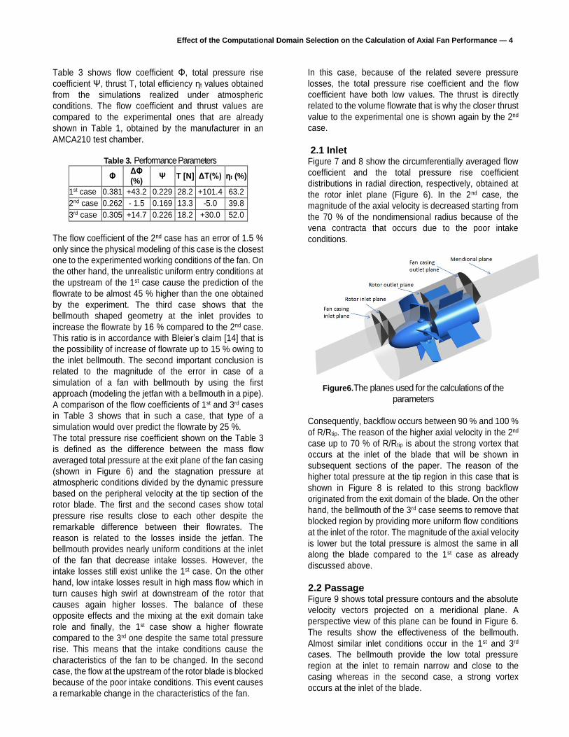
The total pressure rise coefficient shown on the Table 3

is defined as the difference between the mass flow

averaged total pressure at the exit plane of the fan casing

(shown in Figure 6) and the stagnation pressure at

atmospheric conditions divided by the dynamic pressure

based on the peripheral velocity at the tip section of the

rotor blade. The first and the second cases show total

pressure rise results close to each other despite the

remarkable difference between their flowrates. The

reason is related to the losses inside the jetfan. The

bellmouth provides nearly uniform conditions at the inlet

of the fan that decrease intake losses. However, the

intake losses still exist unlike the 1st case. On the other

hand, low intake losses result in high mass flow which in

turn causes high swirl at downstream of the rotor that

causes again higher losses. The balance of these

opposite effects and the mixing at the exit domain take

role and finally, the 1st case show a higher flowrate

compared to the 3rd one despite the same total pressure

rise. This means that the intake conditions cause the

characteristics of the fan to be changed. In the second

case, the flow at the upstream of the rotor blade is blocked

because of the poor intake conditions. This event causes

a remarkable change in the characteristics of the fan.

In this case, because of the related severe pressure

losses, the total pressure rise coefficient and the flow

coefficient have both low values. The thrust is directly

related to the volume flowrate that is why the closer thrust

value to the experimental one is shown again by the 2nd

case.

2.1 Inlet Figure 7 and 8 show the circumferentially averaged flow

coefficient and the total pressure rise coefficient

distributions in radial direction, respectively, obtained at

the rotor inlet plane (Figure 6). In the 2nd case, the

magnitude of the axial velocity is decreased starting from

the 70 % of the nondimensional radius because of the

vena contracta that occurs due to the poor intake

conditions.

Figure6.The planes used for the calculations of the

parameters

Consequently, backflow occurs between 90 % and 100 %

of R/Rtip. The reason of the higher axial velocity in the 2nd

case up to 70 % of R/Rtip is about the strong vortex that

occurs at the inlet of the blade that will be shown in

subsequent sections of the paper. The reason of the

higher total pressure at the tip region in this case that is

shown in Figure 8 is related to this strong backflow

originated from the exit domain of the blade. On the other

hand, the bellmouth of the 3rd case seems to remove that

blocked region by providing more uniform flow conditions

at the inlet of the rotor. The magnitude of the axial velocity

is lower but the total pressure is almost the same in all

along the blade compared to the 1st case as already

discussed above.

2.2 Passage Figure 9 shows total pressure contours and the absolute

velocity vectors projected on a meridional plane. A

perspective view of this plane can be found in Figure 6.

The results show the effectiveness of the bellmouth.

Almost similar inlet conditions occur in the 1st and 3rd

cases. The bellmouth provide the low total pressure

region at the inlet to remain narrow and close to the

casing whereas in the second case, a strong vortex

occurs at the inlet of the blade.

Effect of the Computational Domain Selection on the Calculation of Axial Fan Performance — 5

Figure7.Flow coefficient distributions in radial direction at

the rotor inlet plane

Figure8.Total pressure coefficient distributions in radial

direction at the rotor inlet plane

This vortex blocks the upper part of the blade that causes

the flow to accelerate near midspan of the rotor blade.

The flow conditions at the position of the fan casing outlet

plane (shown in Figure 6) are also remarkable. At the

position of that plane, unlike the results up to now, the 2nd

and the 3rd cases show similar contours in Figure 9. This

time the results of the 1st case is quite different since the

casing of this case is elongated in axial direction that

prevent the mixing of the flow leaving the jetfan with the

atmosphere.

In Figure 10, the pressure contours combined with the

relative velocity vectors projected on a blade-to-blade

surface are shown. This surface is close to the tip region

of the rotor blade corresponding to R/Rtip=0.95 (93 % of

the span starting from the blade root). Most of the relative

velocity vectors in 2nd case seem to be directed to inlet of

the fan that means backflow. Because of this backflow-

swirl combination, the fluid does not flow around the

pressure and suction surfaces of the blade but it hits the

pressure surface somewhere far away from the leading

edge. This stagnation point divides the flow into two

regions. The one which is directed to the exit plane flows

around the pressure surface while the other one is

separated near the leading edge. This results in the

loading of the blade to be decreased in this section of the

blade (Figure 11b). The stagnation points of the 1st and

3rd cases do not occur on the leading edge but are on the

pressure side at a position closer to the leading edge than

the one of the 2nd case. The contours and velocity vectors

are similar in 1st and 3rd cases which have both massive

separations in the suction side. The attached region on

the suction side of the 1st case seems to be larger than

the one of the 3rd case which can be also seen in the Cp

distribution chart in Figure 11b. It is well known that the

area enclosed by the pressure curves of the suction and

pressure sides give the magnitude of the work done by

the blade. Thus, from the charts given in Figure 11b, one

can conclude that the work done by the blade is much

more in 1st and 3rd cases compared to the one of the 2nd

case.

(a)

(b)

(c)

Figure9.Total pressure contours and absolute velocity

vectors projected on a meridional plane: (a) 1st case, (b) 2nd

case, (c) 3rd case.

Effect of the Computational Domain Selection on the Calculation of Axial Fan Performance — 6

(a) (b) (c)

Figure10.Pressure contours and relative velocity vectors on a blade-to-blade plane: (a) 1st case, (b) 2nd case, (c) 3rd case.

(a)

(b)

Figure11. Cp distributions on the blade at (a) R/Rtip=0.7and

(b) R/Rtip=0.95

On the other hand, Figure 11a shows the pressure distribution on the suction and pressure sides of the blade at R/Rtip=0.7 corresponding to 57 % of the blade span starting from the blade root. In this region, the loading of the three cases are more similar compared to the ones of the R/Rtip=0.95. However, one can notice that the suction side of the 2nd case is less loaded which is again a consequence of the vortex at the inlet region and the related backflow at the upper part of the blade that affects the upper-mid span of the blade as well.

2.3 Outlet In Figure 12 and 14, circumferentially averaged flow coefficient and total pressure coefficient in radial direction are shown. The charts on Figure 12 and 14 are obtained behind the rotor and behind the exit of the fan casing, respectively. The results show that the poor inlet conditions affect the loading of the blade which in turn cause the total pressure rise and the axial velocity to be decreased in all along the span.

Figure 13 shows the axial velocity contours just behind the

rotor. A separated region is found in the suction surfaces

near hub region of all the three cases. The axial velocity

contours are similar in that region (can be seen also in

Figure 6) which means that the inlet conditions studied in

this paper do not affect the flow regime near hub region.

However, at the upper radii, low axial velocity values can

obviously be seen in the 2nd case that affects the flow in

midspan region as well. The 3rd case shows that the axial

velocity distribution in upper radii is improved so that low

velocity region is confined to the region near casing.

Effect of the Computational Domain Selection on the Calculation of Axial Fan Performance — 7

(a)

(b)

Figure12. (a) Flow coefficient and (b) total pressure coefficient distributions in radial direction at rotor outlet plane

(a)

(b)

(c)

Figure13.Axial velocity contours at the rotor outlet plane: (a) 1st case (b) 2nd case (c) 3rd case

Figure 14a and 14b shows that in all the three cases, nearly uniform axial velocity distribution in radial direction is provided at the exit plane of the jetfan. Negative total pressure at the wake region of the fan motor of the 1st case in Figure14b differs from that of the 2nd and 3rd cases. This is a consequence of the mixing of the fluid with large domains in 2nd and 3rd cases whereas there is no such a mixing in the 1st case.

(a)

Effect of the Computational Domain Selection on the Calculation of Axial Fan Performance — 8

(b)

Figure14. (a) Flow coefficient and (b) total pressure

coefficient distributions in radial direction behind the fan

casing outlet plane.

CONCLUSION The effect of the computational domain shape on the

aerodynamic performance of a jetfan is investigated.

Three popular domain configurations are studied and the

global parameters as well as the flowfields of these

configurations are investigated and the differences of the

results are discussed. The results show that simulating a

jetfan as if it works in a pipe would bring a considerable

amount of error because of the modified inlet conditions

as well as the lack of the mixing with the atmospheric air

at the exit of the fan. On the other hand, if the jetfan

possess a bellmouth at the inlet to provide uniform inlet

conditions, the error when a simulation is performed as if

the fan works in a pipe is decreased considerably from 45

% to 25 %.

ACKNOWLEDGMENTS The authors would like to thank to Bahçıvan Elektrik Motor

San. ve Tic. Ltd. Şti. for providing the geometry and the

experimental data of the axial flow fan.

NOMENCLATURE

D Diameter, [m] Φ Flow coefficient, [-] Ψ Total pressure rise coefficient, [-] ηt Total-to-total efficiency, [-] Cp Pressure coefficient, [-] T Thrust, [N]

REFERENCES

[1]C. H. Huang and C. W. Gau. An optimal design for axial-flow fan blade: theoretical and experimental studies, Journal of mechanical science and technology, 26(2):427-436, 2012.

[2]G. V. Shankaran, M. B. Dogruoz. Validation of an Advanced Fan Model With Multiple Reference Frame Approach. ITherm2010,Las Vegas, Nevada, USA, 2010. [3]A. Sahili, B. Zogheib, R.M. Barron. 3-D Modeling of Axial Fans. Ima J. Appl. Math, 4:632–651, 2013. [4]M. L. F. Fogal, A. Padilha and V. L. Scalon. Theoretical and experimental study of agricultural spraying using CFD. Journal of the Brazilian Society of Mechanical Sciences and Engineering, 36:125-138, 2014. [5]D. Dwivedi, D. S. Dandotiya. CFD Analysis of Axial Flow Fans with Skewed Blades. International Journal of Emerging Technology and Advanced Engineering, 3(10):741-752, 2013. [6]T. Zhu, T. H. Carolus. Experimental and Unsteady Numerical Investigation of the Tip Clearance Noise of an Axial Fan. Proceedings of ASME 2013 Turbine Blade Tip Symposium & Course Week TBTS2013, Hamburg, Germany, September 30 - October 3, 2013. [7]G. Rábai and J. Vad. Validation of a computational fluid dynamics method to be applied to linear cascades of twisted-swept blades. Periodica Polytechnica, Mechanical Engineering, 49(2): 163–180, 2005. [8]A. Guedel, M. Robitu and V. Chaulet. Energy Efficiency of an Axial Fan for Various Casing Configurations. Journal of Engineering for Gas Turbines and Power, 135(7):074501-1-074501-5, 2013. [9]A. Akturk, C. Camci. A computational and experimental analysis of a ducted fan used in VTOL UAV systems European Turbomachinery Conference, Istanbul, Turkey, March 21-25, 2011. [10]AMCA. Laboratory Methods of Testing Fans for Certified Aerodynamic Performance Rating. Air Movement and Control Association, Arlington Heights,IL, Standard No. ANSI/AMCA 210-07, ANSI/ASHRAE 51/07, 2007.

[11]ANSYS. ANSYS CFX-Solver Theory Guide Release 14.0, ANSYS Inc., Canonsburg, PA, 2011. [12]F. R. Menter. Two-Equation Eddy-Viscosity Turbulence Models for Engineering Application. AIAA J., 32(8):1598–1605, 1994. [13]J. E. Bardina, P. G. Huang, and T. J. Coakley. Turbulence Modeling, Validation, Testing and Development. NASA Technical Memorandum 110446, 1997. [14]F. P. Bleier. Fan handbook: Selection, application, and design. New York: McGraw-Hill, 1998.