Embed Size (px)
Citation preview

Effect of Soil Replacement Option on Surface Deflections for Expansive Clay Profiles
by
Anushree Bharadwaj
A Dissertation Presented in Partial Fulfillment of the Requirements for the Degree
Doctor of Philosophy
Approved April 2013 by the Graduate Supervisory Committee:
Sandra Houston, Co-Chair
Bruno Welfert, Co-Chair Claudia Zapata
ARIZONA STATE UNIVERSITY
May 2013

i
ABSTRACT
Urbanization and infrastructure development often brings dramatic changes in
the surface and groundwater regimes. These changes in moisture content may be
particularly problematic when subsurface soils are moisture sensitive such as
expansive soils. Residential foundations such as slab-on ground may be built on
unsaturated expansive soils and therefore have to resist the deformations associated
with change in moisture content (matric suction) in the soil. The problem is more
pronounced in arid and semi arid regions with drying periods followed by wet season
resulting in large changes in soil suction. Moisture content change causes volume
change in expansive soil which causes serious damage to the structures. In order to
mitigate these ill effects various mitigation are adopted. The most commonly
adopted method in the US is the removal and replacement of upper soils in the
profile. The remove and replace method, although heavily used, is not well
understood with regard to its impact on the depth of soil wetting or near-surface
differential soil movements. In this study the effectiveness of the remove and
replace method is studied. A parametric study is done with various removal and
replacement materials used and analyzed to obtain the optimal replacement depths
and best material. The depth of wetting and heave caused in expansive soil profile
under climatic conditions and common irrigation scenarios are studied for arid
regions. Soil suction changes and associated soil deformations are analyzed using
finite element codes for unsaturated flow and stress/deformation, SVFlux and
SVSolid, respectively. The effectiveness and fundamental mechanisms at play in
mitigation of expansive soils for remove and replace methods are studied, and
include (1) its role in reducing the depth and degree of wetting, and (2) its effect in
reducing the overall heave potential, and (3) the effectiveness of this method in
pushing the seat of movement deeper within the soil profile to reduce differential soil

ii
surface movements. Various non-expansive replacement layers and different surface
flux boundary conditions are analyzed, and the concept of optimal depth and soil is
introduced. General observations are made concerning the efficacy of remove and
replace as a mitigation method.

iii
DEDICATION
This thesis is dedicated to my dear husband Ajatshatru who showed great strength
and support during all these years.

iv
ACKNOWLEDGMENTS
I express my deepest sense of gratitude and reverence towards Dr. Sandra
L. Houston who introduced me to the importance of the subject of Unsaturated Soil
Mechanics and gave valuable guidance and suggestions at all stages of the work
embodied in the present thesis. She critically reviewed and evaluated the whole draft
of the thesis and made valuable inputs in spite of her busy schedule. It was a
rewarding and enlightening experience to have worked under her supervision at all
levels in the fruitful culmination of this endeavor.
I would like to thank Dr. Bruno Welfert for helping me understand the
mathematical implications of the unsaturated soil problem issues and adding value to
my thesis by introducing the numerical aspects of the problem. He also provided his
valuable inputs to this thesis document while reviewing it.
I wish to thank Dr. Claudia Zapata for serving on my committee and providing
insightful suggestions and comments.
I also wish to thank Dr. Kenneth Walsh for providing helpful guidance in the
times of need.
Special thanks to Rob Thode, and Murray Fredlund from SoilVision for their
continuous support with the software.
Last but not the least, I owe a great debt of gratitude towards my parents,
Mrs. Anjali and Dr. S.K. Bharadwaj , a rare blend of kindness, compassion and lofty
virtues for their perseverance, forbearance and endurance during these years of my
absence from home for the acquisition of this knowledge. I am grateful to my elder
brother, Apoorva, who taught me the value of hard work and patience. I also would

v
like to express my love to my younger brother, Anant, for keeping my spirits high
during all these years.
There is a long list of my well wishers to whom I want to extend my sincere
regards and appreciation for helping me learn and accomplish various tasks involved
while working on this research.
A part of this study related to the stability and convergence issues for the
unsaturated finite element solutions was supported by the National Science
Foundation (NSF) under grant number CMMI-0825089. The opinions, conclusions,
and interpretations expressed in this dissertation are those of the author, and not
necessarily of NSF.

vi
TABLE OF CONTENTS
Page
LIST OF TABLES ............................................................................................... x
LIST OF FIGURES ............................................................................................ xi
CHAPTER
1 INTRODUCTION ................................................................................ 1
1.1 Overview................................................................................ 1
1.2 Research Objectives ................................................................ 5
1.3 Scope of the Study .................................................................. 6
1.4 Methodology Adopted .............................................................. 7
1.5 Outline of Thesis ..................................................................... 8
2 REMOVE AND REPLACE MITIGATION SOLUTIONS - A LITERATURE REVIEW
.................................................................................................. 9
2.1 Remove and Replace Mitigation Technique ................................. 9
2.1.1 Depth of Wetting and Active Zone ...................................... 18
2.2 Volume Change Dynamics of Soil and Lightly Loaded Structures
Like Slab-On-Ground ............................................................. 23
3 MOISTURE FLOW AND STRESS-DEFORMATION PDE’S .......................... 26
3.1 Introduction ......................................................................... 26
3.2 Moisture Flow in Unsaturated Soils .......................................... 26
3.3 Head vs. Mixed Formulation .................................................... 28
3.4 Soil Water Characteristic Curve ............................................... 28

vii
CHAPTER Page
3.5 Hydraulic Conductivity Function .............................................. 30
3.6 SVFlux ................................................................................. 32
3.7 Volume Change in Unsaturated Expansive Soils ........................ 34
3.8 Stress-Deformation PDE Solved in SVSolid ............................... 34
4 PROBLEM STATEMENT & BACKGROUND ............................................. 39
4.1 Introduction ......................................................................... 39
4.2 Boundary Value Problems ....................................................... 40
4.2.1 Procedure Adopted to Conduct the Remove & Replace Stress
Deformation Analyses of this Study .................................... 41
4.2.2 Coupling of SVFlux and SVSolid ......................................... 45
4.2.3 General Methodology ........................................................ 46
4.3 Preliminary Problem Set Up .................................................... 47
4.3.1 Mesh Size Selection .......................................................... 49
4.3.2 Time Step Selection .......................................................... 51
4.3.3 Selection of Position of Domain Boundaries ......................... 53
4.4 Final Remove and Replace Problem Set Up ............................... 53
4.4.1 Initial and Final Condition for SVSolid Runs ......................... 56
4.4.2 Mesh Size and Time Steps Used in Final Remove and Replace Study Analyses ................................................................ 56
4.5 Replacement Soils ................................................................. 60

viii
CHAPTER Page
4.5.1 Replacement Layer SWCC and Kunsat Curves ......................... 63
4.5.1.1 Kunsat Function Used .................................................. 64
4.5.2 Soil Properties ................................................................. 66
4.5.3 Degree of Saturation and Suction Values for Replacement Layer
................................................................................. 68
4.6 Climatic Input Data ............................................................... 70
4.6.1 Actual Evaporation Analyses .............................................. 78
4.7 Volume Change Properties in SVSolid ...................................... 84
4.7.1 Plots for Cm variation ........................................................ 85
5 RESULTS & DISCUSSION ................................................................. 89
5.1 Presentation of Results and Discussion ..................................... 89
5.2 Climatic Data Inputs for Roof Runoff Case ................................ 89
5.3 SVFlux and SVSolid Results for Roof Runoff Case ...................... 92
5.3.1 6th Year Results for Lower Ksat Replacement Layer Case ........ 92
5.3.2 6th Year Results for Same Ksat Replacement Layer Case ......... 99
5.3.3 6th Year Results for Higher Ksat Replacement Layer Case ...... 107
5.4 Climatic Data Inputs for Turf Landscape Case ......................... 115
5.5 SVFlux and SVSolid Results for Turf Case ............................... 117
5.5.1 6th Yr Results for Lower Ksat Replacement Layer Case .......... 117
5.5.2 6th Yr Results for 2m Same Ksat Replacement Layer Case ..... 121

ix
CHAPTER Page
5.6 Cm Variation Results ............................................................ 125
5.7 Piecewise Coupled Runs (Turf Case No Replacement Soil) ........ 129
5.8 Implications and Impact of Lateral Flow of Water .................... 132
5.9 Discussion .......................................................................... 138
6 CONCLUSIONS AND FUTURE WORK ................................................. 146
6.1 General .............................................................................. 146
6.2 Recommendation for Future Work ......................................... 147
REFERENCES ............................................................................................... 149
APPENDIX
A CONVERGENCE STUDY RESULTS ..................................................... 156
B 5TH YR CLIMATIC CONDITIONS RESULTS .......................................... 166
C IC AND FC SUCTION PROFILES FOR DIFFERENT DISTANCES FROM SLAB
CENTERLINE ................................................................................. 172
D 1ST PANAM CONFERENCE: EFFECT OF SOIL REPLACEMENT OPTION ON
SURFACE DEFLECTIONS FOR EXPANSIVE CLAY PROFILES .................. 225

x
LIST OF TABLES
Table Page
2.1. Reduction of heave for different cushions (Rao et.al, 2007) – CNS is cohesive
non-expansive soil. ........................................................................................ 12
4.1. Expansive clay properties ......................................................................... 67
4.2. Replacement soil properties ...................................................................... 67
4.3. Placement saturation and suction values for the replacement layer soils ......... 69
4.4. Average Precipitation Data from Phoenix Airport Metrological Station (From
NCDC) (Dye, 2008) ........................................................................................ 72
4.5. Correction factor for different soil types ...................................................... 83
4.6. Typical values for the coefficients of lateral earth pressure (Lytton, 1994) ...... 85
4.7. Volume change Indices for Replacement soils .............................................. 85
4.8. Cm values for each layer ........................................................................... 87
5.1. Heave reduction for different soil and depths of removal and replacement for
Roof Runoff Surface Flux Conditions ............................................................... 140
5.2. Heave reduction for different soil and depths of removal and replacement for
Turf Surface Flux conditions. ......................................................................... 141

xi
LIST OF FIGURES
Figure Page
1.1. Occurrence and Distribution of Potentially Expansive Soil in the United States
(US Army Corps of Engineers, TM 5-878-7, 1977) ................................................ 2
2.1. Plot between swelling potential and thickness of fly ash cushion for different dry densities with 10% cement content (Rao, et al, 2007) ........................................ 11
2.2. Heave –time plots for pavement slabs with cohesive soil cushion (Murthy and
Praveen, 2008) .............................................................................................. 12
2.3. Vertical displacement measures of various depths of inert material at Fort Worth N loop (Lytton et.al, 2004) .............................................................................. 14
2.4. Vertical Displacement Measures of various depths of inert material at Atlanta
US271 (Lytton et.al, 2004) .............................................................................. 14
2.5. Structural distortion of structure resulting from over excavation (Maxwell, 2011).................................................................................................................... 17
2.6. Active zone profile (Nelson and Miller, 1992) ............................................... 19
2.7. Heave occurring in the active zone (Nelson and Miller, 1992) ........................ 19
2.8. Example predevelopment and post development profiles of total suction and the
shifted profiles at three different sites (Walsh et al, 2009) ................................... 22
2.9. Illustration of the soil response to external loads and changes in matric suctions
(PTI, 1996) ................................................................................................... 24
3.1. Typical SWCC curve (after Fredlund and Rahardjo, 1994) ............................. 29
3.2. Relationships between water permeability and matric suction for different soils (Zhan and Ng, 2004) & (Shackelford and Nelson, 1996)...................................... 32
3.3. A typical void ratio constitutive surface plotted in semi logarithmic scale
(Fredlund et al., 2001) .................................................................................... 37
3.4. The total suction is divided into increments and one load increment is applied (Vu and Fredlund, 2001) ................................................................................. 38

xii
Figure Page
4.1. Definition and meaning of a boundary value problem (Fredlund 2006) ........... 41
4.2. em and ym in slab-on-ground foundations .................................................... 45
4.3. Steps to obtain final displacement in SVSolid .............................................. 46
4.4. Initial problem setup ................................................................................ 49
4.5. Suction variation at vertical section X = 10m for various grid sizes (below slab edge) ........................................................................................................... 50
4.6. Roof runoff case boundary condition .......................................................... 54
4.7. Turf case boundary condition .................................................................... 54
4.8. Suction variation below slab edge after 5yr climatic condition run (Initial condition for the Final no replacement profile runs, blow up profile)...................... 55
4.9. 1-D suction variation for different size for no- replacement layer (blow up
profile).......................................................................................................... 57
4.10. 1-D suction variation for different size for Lower Ksat replacement layer (blow up profile) ..................................................................................................... 58
4.11. 1-D suction variation for different size for Higher Ksat replacement layer (blow
up profile) ..................................................................................................... 58
4.12. Suction Time-History plot at 1m depth at various X .................................... 59
4.13. Depth of replacement (cap) for lower conductivity soil ................................ 61
4.14. Depths for different replacement for same and higher conductivity soils ....... 61
4.15. Matrix of runs ........................................................................................ 62
4.16. SWCC for different soils .......................................................................... 64
4.17. Kunsat Curves for different soils ................................................................. 66

xiii
Figure Page
4.18. Initial (IC) and Final condition (FC) suction variation at X=10m, edge of slab (2m same Ksat replacement case) for the roof run-off surface flux condition ........... 69
4.19. Average rainfall ..................................................................................... 73
4.20. PE Data ................................................................................................ 73
4.21. Roof runoff data .................................................................................... 74
4.22. Turf + precipitation data ......................................................................... 74
4.23. Turf data based on daily flux ................................................................... 75
4.24. Turf data based on hourly flux ................................................................. 75
4.25. Temperature data .................................................................................. 77
4.26. RH data ................................................................................................ 77
4.27. Data on the same plot ............................................................................ 78
4.28. The ratio of AE to PE for different soils (Wilson et al. 1997) ......................... 80
4.29. Ratio of AE/PE versus water availability (Holmes, 1961) ............................. 80
4.30. Relationship between relative humidity and total suction using Edlefsen and
Anderson equation, 1943 ................................................................................ 82
4.31. Boundary Conditions in SVSolid ............................................................... 84
4.32. Profile divided into 6 layers ..................................................................... 87
4.33. Cm variation with depth for expansive soil ................................................. 88
5.1. Input Roof Runoff Flux data ...................................................................... 90
5.2. Input Potential Evaporation (PE) and Rainfall data ....................................... 90

xiv
Figure Page
5.3.(a) Initial Condition (IC )and Final Condition (FC) suction profile right below slab edge (see Figure 5.4) - no replacement expansive clay case and roof runoff
conditions. .................................................................................................... 91
5.3.(b) Initial Condition (IC )and Final Condition (FC) suction profile right below slab
edge (see Figure 5.4) - no replacement expansive clay case and roof runoff conditions. .................................................................................................... 91
5.4. Section below slab edge ........................................................................... 92
5.5 (a) Initial Condition (IC )and Final Condition (FC) suction profile right below slab
edge (see Figure 5.4) - for 0.5m lower Ksat replacement case and roof runoff conditions. .................................................................................................... 93
5.5 (b) Initial Condition (IC )and Final Condition (FC) suction profile right below slab
edge (see Figure 5.4) - for 0.5m lower Ksat replacement case and roof runoff
conditions. .................................................................................................... 93
5.6.(a) End of 6th yr suction variation profile below slab edge (see Figure 5.4) for no
replacement expansive clay case and 0.5m lower Ksat replacement material - roof
runoff conditions. ........................................................................................... 94
5.6.(b) End of 6th yr suction variation profile below slab edge (see Figure 5.4) for no
replacement expansive clay case and 0.5m lower Ksat replacement material - roof runoff conditions. ........................................................................................... 95
5.7. (a) Final Displacement results right below slab edge (see Figure 5.4) for no
replacement expansive clay case and 0.5m lower Ksat replacement material - roof
runoff conditions. ........................................................................................... 96
5.7. (b) Final Displacement results right below slab edge (see Figure 5.4) for no
replacement expansive clay case and 0.5m lower Ksat replacement material - roof
runoff conditions. ........................................................................................... 96
5.8. Section at the Ground Surface ................................................................... 97
5.9. Final Displacement variation at the ground surface (see Figure 5.8) for no
replacement expansive clay case and 0.5m lower Ksat replacement material - roof
runoff conditions. ........................................................................................... 98
5.10.(a) Initial Condition (IC )and Final Condition (FC) suction profile right below slab
edge (see Figure 5.4) - 0.75m same Ksat replacement material and roof runoff conditions. .................................................................................................... 99

xv
Figure Page
5.10.(b) Initial Condition (IC )and Final Condition (FC) suction profile right below slab edge (see Figure 5.4) - 0.75m same Ksat replacement material and roof runoff
conditions. .................................................................................................. 100
5.11.(a) Initial Condition (IC )and Final Condition (FC) suction profile right below slab
edge (see Figure 5.4)- 2m same Ksat replacement material and roof runoff conditions................................................................................................................... 100
5.11.(b) Initial Condition (IC )and Final Condition (FC) suction profile right below slab
edge (see Figure 5.4)- 2m same Ksat replacement material and roof runoff conditions.
.................................................................................................................. 101
5.12.(a) Initial Condition (IC )and Final Condition (FC) suction profile right below slab
edge (see Figure 5.4)- 4m same Ksat replacement material and roof runoff conditions.
.................................................................................................................. 101
5.12.(b) Initial Condition (IC )and Final Condition (FC) suction profile right below slab edge (see Figure 5.4)- 4m same Ksat replacement material and roof runoff conditions.
.................................................................................................................. 102
5.13.(a) End of 6th yr suction variation right below slab edge (see Figure 5.4) for no
replacement expansive clay case and replacement cases – same Ksat replacement
material and roof runoff conditions. ................................................................ 103
5.13.(b) End of 6th yr suction variation right below slab edge (see Figure 5.4) for no
replacement expansive clay case and replacement cases – same Ksat replacement
material and roof runoff conditions. ................................................................ 104
5.14.(a) Final Displacement results right below slab edge for no replacement expansive clay case and replacement cases (see Figure 5.4) – same Ksat material and
roof runoff conditions. ................................................................................... 106
5.14.(b) Final Displacement results right below slab edge for no replacement
expansive clay case and replacement cases (see Figure 5.4) – same Ksat material and roof runoff conditions. ................................................................................... 106
5.15 . Final Displacement variation at the ground surface (see Figure 5.8) for no
replacement expansive clay case and replacement cases– same Ksat material and roof
runoff conditions. ......................................................................................... 107
5.16.(a) Initial Condition (IC )and Final Condition (FC) suction profile right below slab edge (see Figure 5.4) - 0.75m higher Ksat replacement case and roof runoff
conditions. .................................................................................................. 108

xvi
Figure Page
5.16.(b) Initial Condition (IC )and Final Condition (FC) suction profile right below slab edge (see Figure 5.4) - 0.75m higher Ksat replacement case and roof runoff
conditions. .................................................................................................. 108
5.17.(a) Initial Condition (IC )and Final Condition (FC) suction profile right below slab
edge (see Figure 5.4) - 2m higher Ksat replacement material and roof runoff conditions. .................................................................................................. 109
5.17.(b) Initial Condition (IC )and Final Condition (FC) suction profile right below slab
edge (see Figure 5.4) - 2m higher Ksat replacement material and roof runoff
conditions. .................................................................................................. 109
5.18.(a) Initial Condition (IC )and Final Condition (FC) suction profile right below slab
edge (see Figure 5.4) - 4m higher Ksat replacement material and roof runoff
conditions ................................................................................................... 110
5.18.(b) Initial Condition (IC )and Final Condition (FC) suction profile right below slab edge (see Figure 5.4) - 4m higher Ksat replacement material and roof runoff
conditions ................................................................................................... 110
5.19.(a) End of 6th yr suction variation right below slab edge (see Figure 5.4) for no
replacement expansive clay and replacement cases - higher Ksat replacement
material and roof runoff conditions. ................................................................ 111
5.19.(b) End of 6th yr suction variation right below slab edge (see Figure 5.4) for no
replacement expansive clay and replacement cases - higher Ksat replacement
material and roof runoff conditions. ................................................................ 112
5.20.(a) Final Displacement results right below slab edge (see Figure 5.4) for no replacement expansive clay case and replacement cases – higher Ksat replacement
material and roof runoff conditions. ................................................................ 113
5.20.(b) Final Displacement results right below slab edge (see Figure 5.4) for no
replacement expansive clay case and replacement cases – higher Ksat replacement material and roof runoff conditions. ................................................................ 113
5.21 . Final Displacement variation at the ground surface (see Figure 5.8) for no
replacement expansive clay case and replacement cases – higher Ksat material and
roof runoff conditions. ................................................................................... 114
5.22. Input Roof Runoff Flux data................................................................... 115
5.23. Input Potential Evaporation and Rainfall data .......................................... 116

xvii
Figure Page
5.24.(a) Initial Condition (IC )and Final Condition (FC) suction profile right below slab edge (see Figure 5.4) - no replacement expansive clay case and turf conditions... 116
5.24.(b) Initial Condition (IC )and Final Condition (FC) suction profile right below slab
edge (see Figure 5.4) - no replacement expansive clay case and turf conditions... 117
5.25.(a) Initial Condition (IC )and Final Condition (FC) suction profile right below slab edge (see Figure 5.4) - 0.5m lower Ksat replacement case and turf conditions. ..... 118
5.25.(b) Initial Condition (IC )and Final Condition (FC) suction profile right below slab
edge (see Figure 5.4) - 0.5m lower Ksat replacement case and turf conditions. ..... 118
5.26.(a) End of 6th yr suction variation below slab edge (see Figure 5.4) for no replacement expansive clay and 0.5m lower Ksat replacement material - turf
conditions. .................................................................................................. 119
5.26.(b) End of 6th yr suction variation below slab edge (see Figure 5.4) for no
replacement expansive clay and 0.5m lower Ksat replacement material - turf conditions. .................................................................................................. 119
5.27.(a) Final Displacement results right below slab edge (see Figure 5.4) for no
replacement expansive clay case and 0.5m lower Ksat replacement material – turf
conditions. .................................................................................................. 120
5.27.(b) Final Displacement results right below slab edge (see Figure 5.4) for no replacement expansive clay case and 0.5m lower Ksat replacement material – turf
conditions. .................................................................................................. 120
5.28. Final Displacement variation at the ground surface (see Figure 5.8) for no
replacement expansive clay case and 0.5m lower Ksat replacement material - turf conditions. .................................................................................................. 121
5.29.(a) Initial Condition (IC )and Final Condition (FC) suction profile right below slab
edge (see Figure 5.4) - 2m same Ksat replacement case and turf conditions. ........ 122
5.29.(b) Initial Condition (IC )and Final Condition (FC) suction profile right below slab edge (see Figure 5.4) - 2m same Ksat replacement case and turf conditions. ........ 122
5.30.(a) End of 6th yr suction variation vertical profile right below slab edge (see
Figure 5.4) - no replacement expansive clay and 2m same Ksat replacement material
and turf conditions. ...................................................................................... 123

xviii
Figure Page
5.30.(b) End of 6th yr suction variation vertical profile right below slab edge (see Figure 5.4) - no replacement expansive clay and 2m same Ksat replacement material
and turf conditions. ...................................................................................... 123
5.31.(a) Final Displacement results right below slab edge (see Figure 5.4) for no
replacement expansive clay case and 2m same Ksat replacement material – turf conditions. .................................................................................................. 124
5.31.(b) Final Displacement results right below slab edge (see Figure 5.4) for no
replacement expansive clay case and 2m same Ksat replacement material – turf
conditions. .................................................................................................. 124
5.32. Final Displacement variation at the ground surface (see Figure 5.4) for no
replacement expansive clay case and 2m same Ksat replacement case – turf
conditions. .................................................................................................. 125
5.33. Cm variation with depth......................................................................... 126
5.34 . Final Displacement variation right below slab edge for no replacement case
(Cm values shown are those at the top of the clay layer only – see Figure 5.33) ... 126
5.35 . Final Displacement variation at the ground surface for no replacement case
(Cm values shown are maximum cm values at the ground surface only – Cm varies
with depth in all cases) ................................................................................. 127
5.36 . Final Displacement variation right below slab edge (see Figure 5.4) for 0.5m
replacement case (Cm values shown are those at the top of the clay layer only – see
Figure 5.33) ................................................................................................ 127
5.37 . Final Displacement variation at the ground surface for 0.5m replacement case (Cm values shown are the maximum Cm values at the ground surface only). ........ 128
5.38. Sequence of run to show piecewise coupled approach to obtain heave results.
.................................................................................................................. 130
5.39. Comparison of suction Variation below slab edge for uncoupled and piecewise coupled runs for 6th yr - no replacement and turf conditions. ............................. 130
5.40. Comparison of displacement variation below slab edge obtained from
uncoupled and piecewise coupled runs - no replacement and turf conditions. ....... 131

xix
Figure Page
5.41. Comparison of displacement variation at the ground surface obtained from uncoupled and piecewise coupled runs - no replacement and turf conditions. ....... 132
5.42. Final Displacement vs. time plot for uncoupled and piecewise coupled runs for
6th yr - no replacement and turf conditions. ..................................................... 132
5.43. Vertical profiles of wetting at 5m, 10m (slab edge), 19m, and 27m from the slab centerline - 0.75m same Ksat replacement material and roof runoff conditions
(blow up profile). ......................................................................................... 134
5.44. Vertical profiles of wetting at 5m, 10m (slab edge), 19m, and 27m from the
slab centerline - 2m same Ksat replacement material and roof runoff conditions (blow up profile). .................................................................................................. 134
5.45. Vertical profiles of wetting at 5m, 10m (slab edge), 19m, and 27m from the
slab centerline - 2m higher Ksat replacement material and roof runoff conditions (blow
up profile). .................................................................................................. 136
5.46. Bathtub effect ..................................................................................... 136
5.47. Vertical profiles of wetting at 5m, 10m (slab edge), 19m, and 27m from the
slab centerline – 0.5m lower Ksat replacement material and turf conditions (blow up
profile). ...................................................................................................... 137

1
1 INTRODUCTION
1.1 Overview
Expansive soils are present all over the world, including the United States. For
decades engineering problems related to expansive soils in many parts of the world
have been reported in the literature (Bao and Ng, 2000), but are generally most
serious in the arid and semi-arid regions. Australia, Britain, Canada, China, India,
Mexico, Spain and United States are some of the countries which must cope with
expansive clays (Fredlund, 1995). Damage to structures in the United States is
commonly related to soil characteristics, with expansive (swell) soils generally
causing the most severe problems. Severe or recurring damage can lower the value
of a house or property. According to the American Society of Civil Engineers, about
half of the houses built each year in the United States are situated on unstable soil,
and about half of these will eventually suffer some soil related damage. According to
Krohn and Slossom (1980), about 20% of the surface soils in United States exhibit
shrink-swell behavior. According to Holtz and Hart (1978), 60% of 250,000 newly
constructed homes built on expansive soils each year in United States experience
minor damage and 10% experience significant damage, some beyond repair. Despite
improvements in performance statistics for new houses built today, expansive soils
remain a significant problem (Coduto, 1999). States like Arizona, California, Colorado
and Texas have a significant extent of expansive soil and, due to the increasing
maintenance costs, a reevaluation of construction and mitigation methods is needed
(Hammerberg, 2006). Figure 1.1 shows the distribution of expansive soil in United
States in 1977.

2
Figure 1.1. Occurrence and Distribution of Potentially Expansive Soil in the United States (US Army Corps of Engineers,
TM 5-878-7, 1977)

3
Local or regional maps showing even more expansive soils region have been
constructed since then (Dye, et al, 2009).
The principal cause of expansive clays is the presence of clay mineral called
Montmorillonite. The presence of Montmorillonite in clay imparts them high swell-
shrink potentials (Chen, 1988). These colloid-sized clay particles have a very large
specific surface area per unit volume and carry negative charge on the surface and
edge. These properties give expansive clays the capability to retain large amounts of
water. Expansive soils are also called moisture sensitive soils because they undergo
substantial volume changes associated with swelling process when subjected to
wetting. As a result, many structures suffer severe damage and distress. The
differential change in expansive soil’s natural water content affects the engineering
property of structures. Therefore, the biggest problem for all the constructed
facilities built on expansive soil is the moisture content change that is associated
with matric suction change.
Residential foundations such as slab-on ground are generally built on
unsaturated soils including expansive soils and have to resist the deformations
associated with change in matric suction in the soil. Matric suction change occurs due
to excessive water exposure over a small area or in a localized fashion due to poor
surface drainage, under pipe leakage or pipe break, heavy irrigation and
infringement of a surface impoundment into joint or bedding features. The amount of
heave occurring in an expansive soil can be represented in a differential form as a
combination of relative changes in suction and net normal stress with appropriate
factors called the volume change indices. Generally, during the swelling process, the
net normal stress state variable remains constant while the matric suction stress
state variable changes due to the wetting process.

4
The hazard posed by expansive soils is greatest in regions with pronounced
wet and dry seasons (Fredlund and Rahardjo, 1993). The swelling phenomenon is
considered as one of the most serious challenges which the foundation engineer
faces, because of the potential danger of unpredictable upward movements of
structures founded on such soils (e.g. Seed et al., 1962; Komornik and David, 1969).
Geotechnical engineering strategies for unsaturated soil zones often incorporate high
degrees of conservatism resulting from assumption of saturated soil properties. On
the other hand, assuming the soil dry throughout the life cycle of design would be
unconservative. Such extreme assumptions in the degree of wetting during the
lifetime of structure have negative implications for design, construction, functionality,
safety and structural longevity (Houston, 2002).
There are various methods/techniques to reduce swelling in soils at the
ground surface to prevent the damage caused to structures. Mitigation measures
may be broadly defined as any actions or designs that lessen or solve moisture
sensitive soil problems (Houston et.al, 2001). Mitigation measures for expansive soil
have been summarized and described by several authors (Clemence and Finbarr,
1981; Chen 1988; Damon P Coppola, 2007; Fredlund and Rahardjo, 1993; Pengelly,
et al., 1997; Nelson and Miller, 1992; Robert W Day, 1999). Among the various
techniques of expansive soil mitigation, remove and replace technique has become
prominent for lightly loaded structures and footings on expansive clays due to its
effectiveness and adoptability. Removal of the upper expansive soil and replacing it
with a non-expansive soil is one such method (IBC, 2006 & IRC, 2006). To
determine whether the option is economical or not, the depth of “active zone” is
determined before the replacement process. However, determination of “active
depth/zone” can be quite challenging, generally requiring some empirical correlations

5
developed for a specific region, perhaps coupled with unsaturated flow analyses.
Engineering practitioners still follow empirical approaches and local experience to
handle the issues related to foundations over expansive clays (Fityus et al., 2004;
Nelson and Miller, 1992; Lytton 1994; Wray 1997; Bratton 1991; Holland and
Richards, 1984; Fredlund and Rahardjo, 1993).
Remove and Replace is widely used in construction practices and people have
proved that it can be an effective technique. Further, several researchers have
considered the mechanisms of remove and replace mitigation in the past. This study
represents a unique investigation on the efficacy of remove and replace methods for
mitigation of expansive soils in that the analyses are based on fundamental
unsaturated flow and stress-deformation principles. These analyses provide a
detailed look into the complexities of the mitigation mechanisms at play for remove
and replace options.
The focus of the study is on the mitigation method of remove and replace and
on the question of effective depth of wetting which will require coupled/uncoupled
flow-deformation analyses using the finite element codes SVFlux and SVSolid using
boundary flux conditions for arid region. This work includes a parametric study of the
characteristics of the replacement (thickness and hydraulic conductivity) to assess
the importance of the replacement soil characteristics on the optimal remove and
replace solution.
1.2 Research Objectives
The intent of this study is to perform a parametric study using uncoupled
flow-deformation analyses to evaluate the effectiveness of the remove and replace
mitigation method for reducing surface deformations in moisture sensitive soils

6
The primary objectives of this study for two different surface flux conditions
(Roof Ponding & Turf) are:
1. To evaluate effectiveness of remove and replace method for reducing
differential heave at ground surface.
2. To study the relative effectiveness of the upper material properties and their
thickness on the depth of wetting and reduction of surface heave of expansive
soils.
3. To better understand best (optimal) replacement materials and depth of
replacement for various surface flux conditions and replacement soil types.
1.3 Scope of the Study
The scope of this study is limited to providing an insight into the impact of
subsurface wetting of expansive soils on surface-reflection deformation through the
use of the finite element solvers SVFlux and SVSolid.
In brief, the scope of the study is:
1. To study the depth and extent of wetting for three different replacement soils
and different replacement depths using SVFlux. Two different surface flux
boundary conditions are considered: roof run-off ponded at the edge of the
structure, and irrigated lawn (turf) conditions.
2. To use stress-deformation finite element analyses (SVSolid) to study the
impact of remove and replace on differential surface heave for three different
replacement soils and different depths using the soil suction changes obtained
from the SVFlux analyses as input.

7
1.4 Methodology Adopted
In order to achieve the objectives of this project, the response of a slab-on-
ground is studied by using finite element software SVFlux for unsaturated flow
analyses and SVSolid for stress-deformation analyses. Two-dimensional stress
deformation analyses of a slab placed on an unsaturated swelling soil using SVFlux
and SVSolid were performed, following the decoupled analysis approach proposed by
Fredlund and Vu (2002). Deformation on the ground surface due to swelling in the
soil was obtained for two different applied flux conditions (ponding of roof run-off
water and irrigated lawn (turf) condition). The upper few meters of the swelling soil
was subsequently replaced by non-expansive soil until a depth of replacement to
study the impact of remove and replace on ground surface movements. SVSolid uses
the soil suction results from SVFlux to determine deformations in soil. It is a
decoupled approach, wherein the time-dependent part of the problem is done using
SVFlux, and then the results are fed into SVSolid to obtain the stresses and
deformations that occur between the initial and final soil suction conditions. In these
analyses the net normal stresses (confining stresses) were held constant. Further,
the slab-on-ground foundation was modeled simply as a flexible impermeable
surface, which does not resist differential heave changes.
The three different replacement layer soil properties for this study were
obtained from the SoilVision database which includes the SWCC and Kunsat data. The
relevant volume change replacement soil properties are based on a literature review
for expansive soils, and on properties determined by others on Arizona expansive
clay (Dye, 2008). The replacement soils are all assumed and modeled to be non-
moisture sensitive (non-expansive), but feature three different saturated hydraulic
conductivity values. Thus 3 different replacement soil types are considered, with (1)

8
same, (2) lesser, and (3) greater saturated hydraulic conductivity compared to the
underlying expansive clay saturated hydraulic conductivity.
1.5 Outline of Thesis
Chapter 1 includes the introduction of the research subject, objective and
scope of the study and outline of the thesis.
Chapter 2 is focused on the literature review of remove and replace technique
and its working mechanism. The theory of active zone and active depth is then
explained, based on definitions presented by different authors in the literature. A
short discussion is included on the volume change dynamics of soil and slab-on-
ground.
Chapter 3 presents the PDE solved by SVFlux and SVSolid. A very brief
summary of moisture flow and volume change in unsaturated soil is also included.
Chapter 4 is a discussion of this research, including the procedure adopted to
conduct this study, coupling of the flow and stress-deformation software and the
problem set up for the remove and replace cases analyzed. Later sections cover
different replacement soil properties, boundary conditions and input fluxes used in
the computer simulations.
Chapter 5 includes results and a discussion of the remove and replace cases
analyzed in the research project, and is followed by conclusions and suggestions for
future study in Chapter 6.

9
2 REMOVE AND REPLACE MITIGATION SOLUTIONS - A LITERATURE
REVIEW
It is a well-known fact that unsaturated expansive soil causes a lot of damage
to earth supported structures due to their shrink/swell behavior in response to soil
moisture (suction) changes. Lightly loaded structures are the worst affected because
the stresses due to structural load do little to prevent heave. There are various
remediation techniques available to mitigate the adverse effects of expansive soils.
Non-structural solutions are aimed at bringing down the swelling potential and the
volume changes in the expansive soil.
Removal of expansive soil and replacement with non-expansive soils is one
method used to mitigate expansive soil foundation materials for slab-on-ground
structures. The most appropriate type of replacement material and its thickness
depend on the climatic factors for a particular region. This chapter includes a
literature review of the remove and replace mitigation technique and its mechanism
in mitigating expansion potential. A brief discussion on the interaction of lightly
loaded structures like slab-on- ground is included at the end.
2.1 Remove and Replace Mitigation Technique
Mitigation of expansive soils can be accomplished in several ways. One of the
ways to avoid the negative effects of expansive soils is to remove some thickness of
expansive soil and replace it with non-expansive soil. Removal of expansive soils and
replacement with non-expansive soils is one method to improve expansive soil
profiles for support of structures (Nelson and Miller, 1992). In some cases, the
expansive strata may be entirely removed. It becomes uneconomical to remove the
entire depth of expansive soil when it extends to a great depth. It then becomes

10
necessary to determine what depth of excavation and fill that is required to reduce
total and differential movements to an acceptable level. Advantages of the remove
and replace are discussed at the end of this section.
The non-expansive soil layer placed over the expansive soil after removal can
provide increased confinement, and thus reduce swell for any expansive soil that
does get wet. Katti (1979) found that if expansive soil layers are covered with a
relatively thin layer of plastic non-expansive soil (clay soil) that the amount of heave
is greatly reduced. He found a clay cap can reduce heave occurring below a depth of
1 to 1.2 m. Furthermore, researchers found that if a layer of expansive soil is
replaced with a soil which does not swell but exhibits some amount of plasticity,
heave at greater depths is reduced. The remove and replace method, using a
relatively thin placement of a clay cap, also reduces the differential heave at ground
due to the reduced hydraulic conductivity of the cohesive soil. Satyanarayana (1969)
and Aly Ahmed (2008) suggested that the entire depth of the expansive soil, or just
a part of the expansive soil in the profile, may be removed and replaced with a “sand
cushion” compacted to some particular dry density, moisture state, and thickness.
However, the “sand cushion method” has several problems if the entire expansive
soil layer is not removed. “The high permeability of sand creates conditions
conducive to easy entry of water from the surface runoff” (Rao et. al, 2007). Rao
et.al, 2007 do not recommend a sand for replacement soil. Figure 2.1 shows the
swelling potential for an expansive soil profile with a fly ash cushion layer varied in
thickness. Thicker replacement layers are more effective in reducing the swelling
potential of the expansive soil (Figure 2.2). Table 2.1 presents the results of the
experiments done by Rao et.al, (2007) comparing the efficacy of different “cushion”
layers in counteracting heave in expansive soils. It was also reported that clay

11
(plastic) replacement soils helps to stabilize expansive soil profiles (Murthy and
Praveen, 2008). Moreover, they concluded that the replacement of upper expansive
soil by cohesionless soils “breaks the cohesive bonds at the interface due to their
different surface properties,” resulting in reduced swell of the profile.
Figure 2.1. Plot between swelling potential and thickness of fly ash cushion for
different dry densities with 10% cement content (Rao, et al, 2007)

12
Figure 2.2. Heave –time plots for pavement slabs with cohesive soil cushion
(Murthy and Praveen, 2008)
Table 2.1. Reduction of heave for different cushions (Rao et.al, 2007) – CNS
is cohesive non-expansive soil.

13
Figure 2.2 shows the decrease in heave with time in the pavement slabs with
different thickness of the cushion layer. It was found that the thickness of the
cushion layer is an important factor influencing the degree of decrease of heave. It is
evident from Figure 2.2 that as the cushion thickness is increased the total amount
of heave is reduced.
Among other remedial techniques, the use of replacement soils below
footings, pavements, linings, and other lightly loaded facilities has been recognized
as an effective and economical approach (Burov, 1977; Katti and Katti, 1994). This
method of mitigation for expansive soils is also mentioned in section 1805.8 of the
International Building Code” (IBC)(2006) for design of foundations on expansive
clay. The IBC document states that the removal of expansive soils should be done to
a depth sufficient to ensure a constant moisture content in the remaining soil profile.
IBC (2006) section R401.4.2 states that the top or subsoils should be removed to a
depth and width sufficient to assure stable moisture content: “The soils removed
may not be used as fill. Instead of a complete geotechnical evaluation, when top or
subsoils are compressible or shifting, they shall be removed to a depth and width
sufficient to assure stable moisture content in each active zone and shall not be used
as fill or stabilized within each active zone by chemical, dewatering or presaturation”.
Lytton et. al (2004) did research on the evaluation of effectiveness of various
design/mitigation procedures for reducing swell and minimizing damage to
pavements. The Lytton study was an evaluation of the effectiveness of replacement
of in-situ subgrade soils with non-expansive soils. Lytton found that replacing the
subgrade with inert (non-expansive) material is effective in reducing the pavement
vertical movement. Figure 2.3 and Figure 2.4 shows how replacing the natural
subgrade can reduce the vertical movement to a considerable degree.

14
Figure 2.3. Vertical displacement measures of various depths of inert material
at Fort Worth N loop (Lytton et.al, 2004)
Figure 2.4. Vertical Displacement Measures of various depths of inert material
at Atlanta US271 (Lytton et.al, 2004)
The remove and replace method has been used for mitigation of expansive
soils in different states like California, Texas and Colorado (California residential code
2010, Texas industrialized building code council 2010, Benson and Associates PC
2005). Removal and replacement of expansive material have been successful in the

15
repair of some hydraulic structures to reduce uplift pressures. Repairs were made on
the Friant-Kearn canal (Holtz and Gibbs, 1956) and the Mohawk and Welton canals
by over excavating the subgrade and replacing the expansive material with sand and
lightly compacted gravel (Holtz, 1959). This remove and replace method also was
also used to reduce expansion of clay by using a thick layer of the remove and
replaced material to increase stress levels on underlying expansive clay. Hotlz (1959)
noted that the differential movement was reduced by the presence of the
replacement gravel layer.
Remove and replace techniques can reduce swelling in expansive soil by four
different mechanisms.
1. First, replacing the upper layer of expansive soil with a lower conductivity soil
will reduce the amount of water infiltrating the soil profile, thereby minimizing
moisture content (suction) change within the profile. As the active zone is
affected by climatic changes and is the region where swelling occurs in
expansive soil, the main objective of this method is to stop water from
entering the profile so that the moisture content remains unchanged due to
the climatic variations.
2. Second, removing the expansive material in the region of wetting reduces the
swelling below the foundation. If the clay exhibits a moderate to low
expansion potential the reduced volume of expansive clay in upper, high
moisture variation layer may be sufficient to prevent large movements at the
surface. However,” if there is a high potential for volume change in the
underlying soil the reduced volume of expansive material may not adequately
prevent surface heave or shrinkage “ (Nelson and Miller, 1992).

16
3. The third mechanism of the mitigating effect of remove and replace is that
heave and differential heave are reduced by moving /pushing the seat of
movement to a deeper depth in the soil profile.
4. Lastly (fourth), the volume change in expansive soil due to wetting gets
reduced by the increased confinement provided by the non-expansive soil
layer, if the thickness of the replacement layer is greater than the removed
layer.
Nelson and Miller also mention the following advantages of the remove and
replace technique:
1. Nonexpansive soils can be compacted at higher densities, yielding higher
bearing capacities than can be produced by prewetting the expansive clay or
compacting it at low densities.
2. The cost of soil replacement can be more economical that other stabilization
procedures since it do not require special construction equipment such as
discs, harrows, mixers or spreaders.
3. Removal and replacement require less delay to construction than some other
procedures such as prewetting.
However, despite all the merits explained above, the remove and replace
strategy can sometimes fail, either because of insufficient removal depth of the
expansive soil or because the replacement soil is highly pervious and causes
structural damage. Non-uniform depths of replacement underneath a structure can
also cause differential movements and increase heave at the ground surface (see
Figure 2.5), (Maxwell, 2011)

17
It is known that pushing the “seat” of wetting deeper into the soil reduces the
swelling feature on the surface (Walsh et.al, 2009). But the effect of remove and
replace mitigation on the depth, degree and rate of wetting is less clear. One reason
is that flow in unsaturated soils, including the determination of soil properties and
characteristics, and their impact on soil deformation is a complex mechanism, which
depends on local soil and climatic conditions.
Figure 2.5. Structural distortion of structure resulting from over excavation
(Maxwell, 2011)
Nelson and Miller (1992) state: “It is very important to recognize the effect of
soil removal, replacement and application of a surcharge on soil microclimate” .When
using granular/sandy soils as replacement layer caution should be exercised as these
are highly permeable soils. Such soils provide access to water for seepage into lower

18
underlying expansive soil layers which could result in heave. It is a general
conception that very low permeability, nonexpansive soils are more satisfactory and
works best as replacement layers. However, there should an optimal soil material
depending on the region climate and other factors which could work as best to
prevent heave.”
2.1.1 Depth of Wetting and Active Zone
Expansive soils swells upon wetting. An important aspect of estimating heave
in soils is the determination of the active depth of wetting. There are different views
and concepts presented by various authors in the literature on depth of wetting
(Walsh, et al, 2009, and associated Journal Discussions). In semi-arid areas
evaporation exceeds the precipitation events or takes place simultaneously. This
balancing process also limits the depth to which pore-water pressure changes can
reasonably occur. The depth of wetting is defined by Nelson et al (2001) as “The
depth to which water contents have increased due to the introduction of water from
external sources, or due to capillarity after the elimination of evapo-transpiration.
The external sources include irrigation, seepage from ponds and others”.
Figure 2.6 shows a general soil profile depicting the various climatic
conditions and active depth. Figure 2.7 illustrates the active zone in an expansive
soil and how heave affects the foundation.

19
Figure 2.6. Active zone profile (Nelson and Miller, 1992)
Figure 2.7. Heave occurring in the active zone (Nelson and Miller, 1992)
Active zone (depth of wetting within the region of the profile where the soil is
expansive) could be only a 2 to 3 ft (0.6 or 0.9 m) deep or could be 15 ft (4.6 m) or
deeper, depending on the climate (Wray, 1995). The active zone thickness is
influenced by the location of groundwater table. If the groundwater table is shallow
(i.e., near the surface), it will tend to keep soil near the surface wetter that it would

20
be if only the climate were influencing the surface soil moisture conditions (Wray,
1995). Conversely, if the groundwater table is deep, it will have a negligible effect on
the active zone and the climate will govern the depth of the active zone. The active
zone depth was found to vary between 1.2 m to 12 m (4 feet to 39 feet) depending
on location (McKeen, 1980, 1981, 1985; O’Neill, 1980; O’Neill and Poormoayed,
1980; Thompson, 1992; Thompson and McKeen, 1995; Wray, 1989, 1997; Wray and
Ellepola, 1991; Durkee, 2000, Chao et al., 2006, Walsh, et al 2009).
“In arid regions like Phoenix, it appears to be the prevailing opinion, that the
top 1.2 to 1.5 m (4 to 5 feet) of soil are the most important for the slab design, with
the active zone depth commonly assumed to be within the upper 1 to 3 m (3 to 9
feet) of the soil profile” (Houston et.al, 2011). The Colorado Association of
Geotechnical Engineers (CAGE) has prescribed a depth of wetting of approximately 6
meters in their guidelines (CAGE, 1996). However, in addition to the findings from
the theories described above, experience indicates that many sites exist where depth
of wetting has greatly exceeded 6 meters (Overton, et al., 2006, and Chao, et al.,
2006). Diewald (2003) evaluated post-construction data from 133 investigations and
determined that the depth of wetting for 7-to-10-year-old residences is
approximately 12 meters. Chen, 1988 recommends a minimum depth of 3 to 4 ft for
remove and replace. Usually sub excavation can be applied practically to a The active
depth is the depth up to which changes in the pore-water pressure are likely to occur
under given climatic conditions (Fredlund et al. 1993). Generally most of the heave
occurs in near ground where maximum change in pore pressure occurs under no
confinement. Precipitation or infiltration events cause a lowering of suction levels in
the soils. However swelling soils have high clay content and as a result have low

21
hydraulic conductivity which limits the ability of the soil to transfer excess water to
lower depths.
Nelson et al (2001) ; Nelson, Durkee and Bonner(1998); Durkee (2000)
define the active zone as the zone of soil that contributes to heave due to soil
expansion at any particular time and it varies with time. Wetting depth due to
climatic conditions is shown in Figure 2.6.
Walsh et al. (2009) developed a site specific approach for the Denver
metropolitan area to assess the depth of wetting. In this method the average pre-
development suction trend line and post-development suction profile of the region is
obtained first and then the trend line is shifted to obtain a best fit with the lower
portion of the post-development profile. The depth of wetting is then defined as the
depth to which the post-development suctions are significantly lower than the shifted
suction profiles (Figure 2.8).
McOmber and Thompson (2000) method to estimate wetting depth is based
on the difference between the post development and predevelopment suction
profiles. Below that profile, an equilibrium suction exists. In the same study done in
Denver region, the depth of wetting estimated by varies authors is different
according to the approach adopted by them. McOmber and Thompson (2000)
estimated a depth of wetting for that area around 6-9m, while of Nelson et al.
(2001) estimated it to be about 15-28m.
Thompson (1997) and McKeen (2001) assume that an equilibrium suction
profile exists below the depth of wetting. At the surface the suction fluctuates due to
the climatic conditions. This approach has been used in their methods to evaluate
heave below foundations.

22
Figure 2.8. Example predevelopment and post development profiles of total
suction and the shifted profiles at three different sites (Walsh et al, 2009)
Thompson (1997) developed two approaches, swell testing and suction
measurement, to calculate potential future heave. McKeen (2001) mentioned that
the plot of suction versus depth is the direct method to estimate the active zone
depth which has been used in his method to calculate heave.
The climatic conditions of a region usually are the controlling factors of the
active zone. In particular the maximum possible soil moisture seasonal changes
impacts the suction profiles during wet and dry seasons. The expected swelling
pressures as well as differential soil movement are dictated by these seasonal
changes in suction or moisture content of the soil. Hence, for a geotechnical engineer
dealing with expansive soil, it is very important to have knowledge of the soil suction
distribution in the soil. Therefore, the engineering behavior (i.e., heave and

23
shrinkage) of the soil is easier to manage if the seasonal soil suction distribution for
a site with expansive soil is known. Consequently, there is a need for a proper basis
to obtain an optimum replacement depth, based on flow-deformation analyses. Also,
the actual wetting depth and active zone required in the design of slab-on-
ground/foundations for lightly loaded structures should be identified and evaluated to
avoid such failures.
2.2 Volume Change Dynamics of Soil and Lightly Loaded Structures Like
Slab-On-Ground
The interaction between a slab-on-ground foundation and soil volume
changes in expansive soil is quite complex. This whole system can be viewed as
consisting of interactions between the soil and the structure.
The assessment of the variables, maximum ground surface movement in the
absence of the slab, ym, and horizontal distance of moisture movement beneath the
slab, em are commonly reported parameters used in structural design of slab-on-
ground foundation. A typical example of edge lift and center lift (edge drop) on a
slab on ground under various climatic factors and external load is shown in Figure
2.9.

24
Figure 2.9. Illustration of the soil response to external loads and changes in
matric suctions (PTI, 1996)
Evaluation of slab on grade performance on expansive soils profiles can be
studied using unsaturated flow and unsaturated soil stress- deformation analyses.
Several finite element codes are available to solve the governing partial differential
equations for flow/deformation, including SVFlux and SVSolid used in this study.
Remove and Replace technique is very commonly used in foundation and
other construction practices. Several authors have reported in the literature about its

25
effectiveness and adaptability. However, the efficacy of this method has not been
analyzed extensively from a fundamental unsaturated soil moisture flow and stress-
deformation perspective. This is an investigation on the remove and replacement
method for mitigation of expansive soils in which the analyses are based on
fundamental unsaturated flow and stress-deformation principles. Thus, this research
represents a new and unique contribution to the state of knowledge on remove and
replace methods.

26
3 MOISTURE FLOW AND STRESS-DEFORMATION PDE’S
3.1 Introduction
This chapter presents a brief overview of the theory of moisture flow in
unsaturated soil and the partial differential equation (PDE) solved in SVFlux. The
next section includes a general theory on volume change in unsaturated expansive
soil and the stress-deformation PDE solved by SVSolid for modeling suction and net
normal stress induced deformation in unsaturated expansive soils.
3.2 Moisture Flow in Unsaturated Soils
As with the flow of water through saturated soils, flow of water through
unsaturated soils is governed by gradients in total fluid potential (hydraulic head).
In general, the hydraulic head consists of three components: gravitational
head, pressure head, and kinetic head. The total hydraulic head can be written
3.1
where
= elevation [m]
= pore water pressure [kPa]
= flow velocity [m/s]
= specific weight of water [kN/m3]
= acceleration due to gravity [m/s2]

27
In the present study is small and only the first two components (elevation
and pressure heads) are used.
The governing PDE for moisture flow through unsaturated soils for 2D
unsaturated flow is given by Richard’s equation (Equation 3.2)
3.2
where
x and y are the horizontal and vertical directions, respectively,
Θ is the volumetric water content [dimensionless],
kw (Θ) is the two dimensional hydraulic conductivity function which provides the
relationship between the hydraulic conductivity or volumetric water content and the
matric suction [m/day]. The hydraulic conductivity is generally a function of the
suction or, equivalently, the head.
Similarly kvd represents a scalar vapor conductivity function for the vapor phase. This
term only contributes at relatively large suctions.
The dependent variable Θ is related to the suction ua-uw difference between
air and pore water pressures) via the soil water characteristic curve (SWCC), which
depends on the soil characteristics. The suction ua-uw is itself related to the head H
via Equation 3.1.
Both SWCC and hydraulic conductivity functions are discussed in more detail
below.

28
The SWCC, hydraulic conductivity, and the vapor conductivity of soil tend to
change with suction and therefore make the unsaturated flow equation nonlinear.
3.3 Head vs. Mixed Formulation
The moisture flow equation involves moisture content, total head and,
implicitly, pore water pressure. Because these quantities are related to each other
Richard’s equation (Equation 3.2) can be written in terms of any single one of them
exclusively. The head-based form is most commonly used but suffers poor mass
balance in transient problems. This problem becomes even worse in problems with
highly nonlinear soil water characteristic curves. For this study, the mixed form
Equation 3.2 (Celia, 1990) involving both water content and pressure head is used.
It has the advantage of improved mass-balance errors over head- based form.
3.4 Soil Water Characteristic Curve
One of the property functions required for unsaturated flow modeling is the
soil water characteristic curve (SWCC), which describes the relationship between soil
water content () and soil suction ua - uw.
A typical SWCC is shown below in Figure 3.1.

29
Figure 3.1. Typical SWCC curve (after Fredlund and Rahardjo, 1994)
The various material properties that affect the general shape of SWCC for
various soils include pore size distribution, grain size distribution, density, organic
material content, clay content and mineralogy.
The several defining features of the SWCC curves are shown in the
Figure 3.1 above. The most important of these are the saturated volumetric
water content, air entry value (AEV), and residual water content. At zero suction the
soil is fully saturated. As suction increases water content remains about constant
until the air manages to penetrate the soil pores. So the corresponding suction value
is the air entry value (AEV). As suction continues to increase the water content
decreases until it reaches a residual value corresponding to a residual film
surrounding soil particles. SVFlux provides different fits to estimate the SWCC for
soils. For this study, the Fredlund and Xing (1994) fit was used for all soils. The fit is
given by the equation

30
3.3
where
Θw = volumetric water content at any soil suction
Θs = saturated volumetric water content
a = a material parameter which is primarily a function of air entry value of the soil in
kPa
n = a material parameter which is primarily a function of rate of water extraction
from the soil once the air entry value has been exceeded
m = a material parameter which is primarily a function of the residual water content
uw = ua-uw = soil suction
uwr = suction at which residual water content occurs (kPa)
When cycling through wetting and drying conditions possible hysteresis can
occur but has not been considered in this study.
3.5 Hydraulic Conductivity Function
The other important soil property is its hydraulic conductivity which is also a
function of either head, water content, pore water pressure, or suction. Saturated
and unsaturated hydraulic conductivity are both related to the degree of resistance
from soil particles when water flows in the soil pores. It is also a function of material
variables describing pore structure i.e., void ratio and porosity; pore fluid properties
i.e., density and viscosity. The hydraulic conductivity of an unsaturated soil can vary

31
considerably during a transient process as a result of changes in the volume-mass
properties.
A typical plot of unsaturated hydraulic conductivity for different soils as a
function of suction is shown below in Figure 3.2. It can be observed that the
hydraulic conductivities are different for different soils at the same volumetric water
content. This difference is due to the differences in water configurations in individual
soils.
Near saturation (at low suction) the coarse grained soils have higher
conductivity than fine grained soil. However, when destaurated, the conductivity in
the coarse grained soils decreases faster than in fine grained soil, resulting in a
cross-over point. Beyond that point the hydraulic conductivity of the coarse grained
soil remains lower than the fine grained soil. Such cross-over did in particular occur
in our remove and replace strategy between the higher conductivity replacement soil
and the original clay.
As the soil dries, there is less water in the voids and the hydraulic
conductivity decreases. This effect also affects the rate of evaporation occurring
across the soil surface.

32
Figure 3.2. Relationships between water permeability and matric suction for
different soils (Zhan and Ng, 2004) & (Shackelford and Nelson, 1996)
3.6 SVFlux
The commercial software package SVFlux was used for the analysis of the
“remove and replace problem” considered in this study. SVFlux (Soil Vision Ltd.2009)
is a seepage analysis package which is capable of solving 2D and 3D problems under
either steady state or transient conditions. SVFlux implements both head based and
mixed formulations of the Richard’s equation (Equation 3.2).
SVFlux is based on the general purpose PDE solver FlexPDE, which can handle
highly nonlinear PDE problem, such as water flow in unsaturated soils. FlexPDE
allows piecewise linear or quadratic finite element spatial discretization. It has a
feature for automatic mesh generation and adaptive grid refinement.

33
Time integration of the time dependent Richard’s Equation 3.2 is typically
performed using an implicit scheme based on backward differentiation (BDF). This
results in a system of nonlinear equations which are solved using a Newton-Krylov
type iteration. The software also includes adaptive time stepping.
SVFlux allows application of both natural (Neumann/Flux) and essential
(Dirichlet/Head) boundary conditions. Dye (2008) performed various sensitivity
studies to evaluate the stability performance of solutions for fixed time steps and
reported that tighter mesh spacing reduces the magnitude of oscillations induced in
the results for applied Neumann boundary conditions (infiltration flux problems).
Appropriate time steps and mesh sizes should be selected to obtain stable and
converged solution. She also found that in case of problems involving runoff at the
surface should be solved using tighter mesh sizes, as runoff induces oscillations in
the simulations.
Dye also found that the numerical solutions are sensitive to the variability in
the hydraulic conductivity functions in unsaturated soils. Therefore the hydraulic
conductivity of soils, especially for lower conductivity soils, can have impacts on the
stability and convergence of the problem solution. To ascertain convergence of the
solution, global error parameters of the solver would be varied to check the
sensitivity of the results to these variations. This is discussed in detail in Chapter 4
for the analyses performed in this research.
SVFlux offers various fits to estimate the kunsat curve for soils. The Leong and
Rahardjo fit (1996) was used to define the kunsat curves for all the replacement soils
in this study.

34
3.7 Volume Change in Unsaturated Expansive Soils
Generally in a volume change analysis, both the net normal stress and matric
suction must be considered.” There are three primary factors that affect the total
heave prediction, namely, the volume change indices and the present and the future
stress state variables” (Fredlund, 1993). The amount of volume change in an
expansive soil can be written as function of the difference between the present stress
state and the future stress state and the volume change indices for the soil.
Generally the net normal stress state variable remains constant while the matric
suction stress state variable changes during the swelling or shrinkage process. For
the different surface flux cases analyzed in this study, an uncoupled approach was
used which involves the coupling between SVFlux and SVSolid. The details of how
SVFlux and SVSolid are combined to obtain deformations resulting from unsaturated
flow analyses for unsaturated expansive soils are discussed in Chapter 4.
3.8 Stress-Deformation PDE Solved in SVSolid
SVSolid Standard 6.0, used in this study, is a finite element package capable
of solving stress-strain models for unsaturated soils (SVSolid manual, 2008). Like
SVFlux, it also has the feature of automatic mesh generation to solve highly
nonlinear problems. As in SVFlux, SVSolid also implements a Newton type iteration
for solving the nonlinear PDE’s for stress-deformation (SVSolid manual, 2008).
SVSolid offers different stress strain constitutive models like linear elastic
model, anisotropic model, hyperbolic model and unsaturated model. SVSolid can
perform both total stress and effective stress analysis depending upon the type of
problem.

35
The governing PDE relates the displacements u and v in the x and y direction
respectively to the pore water ua –uw obtained from SVFlux according to the
isotropic, nonlinear elastic soil model (Vu and Fredlund, 2004):
3.4
3.5
where
bx and by are body forces in x and y directions respectively
by is the body load in vertical direction to incorporate the effect of gravity or
overburden load
bx is the body force in horizontal direction and are calculated based on the coefficient
of earth pressure at rest
3.6
3.7
3.8
3.9
For a 2D plane strain case, Elasticity parameters are given by:

36
3.10
3.11
where
E is the elasticity parameter for the soil structure with respect to a change in net
normal stress
H is an elasticity parameter for the soil structure with respect to a change in matric
suction
μ is the Poisson’s ratio for the soil structure and
eo is the initial void ratio
Equations 3.4 and 3.5 are used to compute the displacements in horizontal
and vertical directions due to a change in matric suction obtained from SVFlux. Cm
and Cs are the swelling indices, i.e. the slopes of the void ration versus logarithm of
net normal stress and logarithm matric suction respectively. Figure 3.3 shows the
variation of Cm and Cs as used in SVSolid.

37
Figure 3.3. A typical void ratio constitutive surface plotted in semi logarithmic
scale (Fredlund et al., 2001)
The elastic moduli E and H are calculated based on the Cs and Cm. Lower Cm
values result in an increase of the elastic modulus (H) with respect to suction,
resulting in a reduction in final displacement value obtained from the PDE. In
general, the Cm value decreases with increasing confinement because increased
confining stresses act to “hold the soil down” and reduce swell upon wetting.
The unsaturated model option in SVSolid is used in this study to solve for the
problems involving stress-deformation analyses. An initial suction profile is obtained
by running a transient simulation with SVFlux until the solution stabilizes. Next a
final suction profile is obtained by another transient simulation using desired
boundary conditions for a number of years (6 years for this study using climatic
conditions). The initial and final suction profiles are provided directly to SVSolid. The
software interpolates between these two profiles at a number of stages (see Figure
3.4) from which it obtains small variations in suction profiles. Corresponding

38
incremental deformations are then obtained from Equations 3.4 and 3.5. “During
each incremental step, the elastic moduli are assumed to be unchanged” (Vu and
Fredlund, 2001). Then, “new moduli are selected at the beginning of each new
incremental step depending upon the stress level and the displacements from each
incremental step are accumulated to give total displacement” (Vu and Fredlund,
2001). The overall strategy can be interpreted as continuation technique via
linearization and accumulation of incremental deformations.
Figure 3.4. The total suction is divided into increments and one load
increment is applied (Vu and Fredlund, 2001)

39
4 PROBLEM STATEMENT & BACKGROUND
4.1 Introduction
The objective of the research is to study the effect of remove and replace
options for mitigation of expansive soil profiles for shallow foundation structures.
Removal of expansive soils and replacement with non-expansive soils is one method
to reduce expansion potential of a clay profile. In some cases, the expansive strata
may be entirely removed. It becomes uneconomical to remove the entire depth of
expansive soil when it extends to a great depth. It then becomes necessary to
determine the optimal depth of excavation and fill required to reduce heave to an
acceptable level. The details of different remove and replace cases, whose strategies
were outlined in chapter 2, are presented in Section 4.5 of this chapter. The study of
optimal replacement depth and material is accomplished using two commercial
softwares, SVFlux and SVSolid (SVOffice 2009). Dye (2008) performed a detailed
study on moisture flow through expansive soil, including a study of the effect of time
and space discretization on the numerical stability and convergence of the problem
of infiltration into expansive clays. Since the Dye study, several revisions have been
added to the SVOffice software to improve the stability of numerical solutions in
particular for stiff problems. In this study, the solutions presented for the remove
and replace problem were evaluated for stability and convergence, and iterations on
discretization in time and space were done for 1D models in obtaining and
appropriate finite element solutions; then these discretizations were checked for the
2-D case. Only the final stable and converged solutions are presented in the body of
this dissertation, although several iterations on discretization were required to obtain
satisfactory solutions. The 2D problem analyzed is described in the sections below,
including initial conditions, and various boundary conditions considered. The Soil-

40
Water Characteristic Curve (SWCC) and Kunsat functions used for the expansive and
replacement soils are also presented and discussed. Overall this chapter describes
the problem setup and the various soil properties considered for the replacement soil
layers, as well as properties selected to represent the natural expansive clay profile
to be mitigated.
4.2 Boundary Value Problems
The finite element analysis for swelling problems in unsaturated soil
mechanics is done by solving stress-strain partial differential equations (PDE’s) for
soil equilibrium using unsaturated flow PDE’s (Richards Equation) solutions. This may
be done in a coupled or uncoupled manner. The governing partial differential
equations used in this study for both fluid flow and stress deformation are based on
the general theory of unsaturated soils using two independent stress-strain variables
(Vu and Fredlund 2002). As discussed by Fredlund (2006), the solution to the flow
and stress-deformation equations for specific site conditions can be viewed as a
boundary value problem, as shown in Figure 4.1. When a head value is specified for
flow type problems it is called a Dirichlet boundary condition. The specification of
flow rate across a boundary results in Neuman type boundary condition. Both types
of boundary conditions must be considered in the study of expansive soils for field-
appropriate conditions.
The volume changes associated with expansive clays can be predicted as the
solution of a stress-deformation analysis using the fluid flow analyses for
determination of soil suction changes (Vu and Fredlund 2002). In the analysis
proposed by Vu and Fredlund for expansive soils, and used in the SVSolid software,
the soil properties are generally nonlinear but are converted to equivalent,

41
incremental elastic parameters. The swelling index is converted to an equivalent
variable elasticity function for the unsaturated soil (Vu and Fredlund, 2002). For
expansive soils, the volume change occurs in response to changes in soil suction,
typically for constant, or essentially constant, net normal stress conditions.
Figure 4.1. Definition and meaning of a boundary value problem (Fredlund
2006)
4.2.1 Procedure Adopted to Conduct the Remove & Replace Stress
Deformation Analyses of this Study
The methodology adopted in this study is summarized as below:
1. A decoupled analysis is performed, wherein the unsaturated flow analysis is
first solved and then used as input to the stress-deformation analysis of the
expansive clay. In the SVSolid software there is a piecewise one-way coupling
such that the changes in soil suction associated with the fluid flow analysis
are used to compute deformations that result in changes in net normal stress.
The changes in net normal stress are not used to compute changes in soil
suction.

42
2. The conditions for climate conditions plus development-induced flow (e.g.
irrigation, roof run-off, etc) on the unmitigated expansive soil profile
condition, in the absence of removal and replacement, are evaluated to
establish a baseline condition for comparison to remove and replace options.
An unsaturated fluid flow analysis model (i.e., SVFlux) is prepared
for the expansive clay soil profile to obtain the pore water pressure (soil
suction) conditions for natural climatic conditions. To establish the initial
conditions the soil profile is subjected to 5 years of natural climatic conditions,
which was found to provide essentially pseudo-steady-state conditions for the
profile (steady other than seasonal fluctuations). These analyses establish the
initial condition for the no replacement case. Next, transient (e.g. irrigated
lawn conditions, or roof runoff ponding conditions) are analyzed to establish
the final boundary condition for the deformation analyses (SVSolid) for the no
replacement case. The stress-deformation model using SVSolid provides
deformations associated with the changes in matric suction. The soil profile is
divided into different layers to incorporate the variation of matric suction
volume change index, Cm, with depth (see Figure 4.33). The soil properties
for the native clay are for an actual expansive soil, although the variation of
Cm with depth is estimated based on experience and literature values. Cm is
the slope of the void ratio vs. suction plot on a semi logarithmic scale (see
Figure 3.3). The entire deformation pattern is determined in the finite
element analyses, but deformation below the slab edge and ground surface is
captured for plotting in this study for comparison of the efficacy of various
remove & replacement depths, as described briefly in Chapter 3 and
discussed in detail in the subsequent sections of this chapter.

43
3. After the soil deformation pattern is obtained for the natural, unmitigated soil
profile, the fluid flow model is rerun but with the top layer of the expansive
soil profile removed and replaced with non-expansive soils. For each run, the
replacement layer for this study consists of one of three different artificial
non-expansive soils with varying hydraulic conductivities compared to that
native clay – higher than, lower than, or equal to the native clay conductivity.
For the non-expansive soils, reasonable volume change properties are
estimated based on the literature values on compacted soils. Details are
provided in subsequent sections of this chapter. The unsaturated flow analysis
(SVFlux) is performed for the two layered soil model with the top layer of the
natural clay profile replaced with various non-expansive soils. The flow
analyses conducted using SVFlux are followed by a 2D deformation analyses
using SVSolid for each remove and replace case.
The soil suction variation and changes in degree of saturation are obtained
from the unsaturated analysis (SVFlux). Time history plots for saturation and
suction are captured and saved for subsequent evaluation at various defined
points along the x and y axes within the domain of the soil profile. These
points lie on a grid and are spaced at a distance equal to the grid size,
concentrated mostly in the region near to the surface where suction changes
occur. The grid points are distanced more sparsely as the depth below ground
surface increases. Also, plots for suction and saturation are obtained for
various depths below the slab edge for subsequent evaluation of the model
results. Thus, horizontal and vertical profiles of soil suction and degree of
saturation may be plotted for comparison between the various remove and
replace options and for the two selected surface boundary conditions (roof
run-off or turf (lawn).

44
Finally, results are plotted in terms of vertical profiles of displacement below
slab edge, horizontal profiles of displacement on the ground surface to
estimate the differential settlement occurring across the slab. The slab itself is
not modeled, except to serve as a flexible impermeable member. Thus, the
displacements represent soil movements and do not consider soil-structure
interaction effects.
4. Comparisons are made between the various remove and replace options. A
matrix showing all of the conditions considered and compared in this study is
shown in Figure 4.15, later in this chapter.
5. Finally displacement (primarily heave) results are interpreted in terms edge
moisture distance (em) and differential movement (ym) for slab (see Figure
4.2). The magnitude of ym refers to soil movements that would occur in the
absence of the slab. The edge moisture variation distance refers to the
distance inward from the edge of the slab that the soil moisture content can
be expected to vary.

45
Figure 4.2. em and ym in slab-on-ground foundations
4.2.2 Coupling of SVFlux and SVSolid
The primary cause of volume change in the current problem is the change in
soil suction. The fluid flow analysis is the initial and most important step to
determining the overall volume change. The initial and final conditions (from SVFlux
analyses) are selected each time manually for input into SVSolid depending at what
time the final displacement value is needed. The manual iteration method involves
steps (explained below) to arrive at the final displacement using SVFlux and SVSolid
software packages. These software packages utilize the FlexPDE generic finite
element solver to solve the partial differential equations for flow and stress-
deformation. The steps are described as below:
1. Initial SVFlux seepage analysis
2. Final SVFlux transient seepage analysis
3. SVSolid Stress/deformation analysis

46
The purpose of the initial seepage analysis in SVFlux is to get 2 outputs:
1. A head profile to use as initial conditions for the final transient seepage
analysis
2. To obtain a suction profile to use as initial conditions for the SVSolid analysis.
The Final Transient SVFlux analysis provides an output of suction variation
within the profile at a given time, which becomes the final condition input into
SVSolid. SVSolid then uses these initial and final suction profiles to compute the
deformations induced due the change in suction.
The flow chart (Figure 4.3) below explains the process to obtain the final
displacement values for the moisture change problems.
Figure 4.3. Steps to obtain final displacement in SVSolid
4.2.3 General Methodology
In order to achieve the objectives of this project the response of a slab-on-
ground by using SVFlux for seepage analysis and SVSolid for stress-deformation
analyses is studied. A two dimensional stress deformation analysis of a slab placed
on an unsaturated swelling soil is performed using SVFlux and SVSolid packages is
done which follows the decoupled analysis approach proposed by Fredlund and Vu

47
(2002). Deformation on the ground surface due to swelling and/or shrinkage in the
natural, unmitigated soil was obtained for two different applied surface flux
conditions, roof run-off ponded at the slab edge or turf (lawn) landscape conditions.
Then the upper few meters of the swelling soil was replaced by non-expansive soil to
a given depth of replacement, to determine the impact of the remove and replace
mitigation scheme. SVSolid uses the seepage analysis results from SVFlux to
determine stress and deformation in soil. It is a decoupled approach where the time
dependent part of the problem is done using SVFlux and then the initial and final soil
suction results are fed into SVSolid to obtain the stresses and deformations after a
particular time (final condition).
The three different replacement layer soil properties for this study were
obtained from the SoilVision database. This database includes the SWCC and Kunsat
data for various soils. The relevant replacement soil volume change properties are
based on a literature review. The volume change index with respect to suction, Cm,
varies with depth for the expansive clay layer, and the variation with depth was
estimated primarily from oedometer test results on compacted soils presented by
Miller, 1992) (see Figure 4.33).
4.3 Preliminary Problem Set Up
A preliminary study was conducted to obtain optimal space and time
discretization values and to study appropriate placement of edge and base
boundaries so as to not affect the solution in the zone of interest around the slab.
The preliminary problem consisted of a 2D soil profile 7 meters deep and 20m wide.
The initial condition for the problem was a head of -153m applied over the entire soil
profile. The initial condition head value used in the analyses is based on the desert

48
region suction values typical of the Phoenix, Arizona region, as reported by Dye
(2008). With this initial condition, steady state analysis was done in SVFlux for the
problem to obtain a hydrostatic head profile and a suction profile. The head profile
obtained from this run was used as an initial condition for the subsequent transient
analysis in SVFlux. The subsequent transient run in SVFlux is done with roof runoff
data applied on the top boundary of the soil profile (over a region of 1m), allowing
for approximately 5 inches of ponding to occur, with the remainder run off. This
transient SVFlux run also generates a suction profile. The suction profile obtained
from the steady state run was used as the initial condition for the SVSolid analysis
and the final condition for SVSolid is obtained from the subsequent transient SVFlux
run. For the transient analysis in SVFlux, the boundary value consists of a head -
153m applied at the bottom boundary of the domain, and a zero (no) flux condition
is applied on both lateral sides. On the top boundary, a slab-on-ground covers half
the boundary length and a flux consisting of average yearly roof runoff data (Figure
4.21) was applied over a concentrated area of length of 1 meter as shown in the
Figure 4.4 below. The details of the climatic data are given in Section 4.6. For the
preliminary stability and convergence studies an average flux was used, although for
the final analyses hourly flux steps were used to obtain a more accurate description
of the surface flow conditions as averaging of surface flux has been found to over-
estimate depth and extent of wetting (Dye, et al., 2008)
Once the change between initial and final suction is obtained for the soil
profile, it is used to obtain the data required for plots of the vertical movement (or
the amount of swelling at the surface) and profiles of suction below slab edge using
SVSolid. The coupling between the two softwares is explained in Section 4.2.2.

49
Figure 4.4. Initial problem setup
The problem set up presented in this study is geometrically axisymmetric and
therefore only half of the soil profile was analyzed.
4.3.1 Mesh Size Selection
Boundary flux modeling with different flux conditions is complex and
challenging from numerical and convergence perspectives. Therefore an optimum
mesh size is necessary in order to obtain stable solutions that run in a reasonable
length of time. The number of nodes/mesh density, and Δt (time), was varied using
different mesh spacing in SVFlux so as to compare the results and check for
convergence. “In a given numerical problem the number, shape and density of
elements used effects the computational expense and accuracy of solution” (Vu,
2002). The accuracy of finite element solution depends on the choice of the finite
element mesh. As the size of the finite element mesh gets smaller, in general, the
accuracy of the solution increases. Because a finer mesh size adds to the solution
times of the problem, the selection of mesh size and time discretization is an
important part in the optimization process. For the initial problem set up, different

50
mesh sizes were used on the “no replacement” expansive soil profile in order to
obtain stable results in SVFlux. A separate convergence study was done to find out
the appropriate Δx and Δt for the expansive clay profile runs. A result for suction
variation for a vertical profile at the edge of the slab, for various different grid sizes,
is shown below in Figure 4.5. Additional saturation and suction results for different
grid size are included in Appendix A. The software code gives the option to the user
to manually control the mesh density or use the regrid option. If the regrid option is
chosen the PDE solver implements adaptive mesh refinement. The solver
automatically refines the mesh (produces more nodes) in the region where the
specified error limit is exceeded. This process allows a specified accuracy to be
achieved. This option can be turned off and a fixed mesh can be chosen. In this
section the effect of the adaptive mesh and fixed mesh on the suction results are
discussed.
Figure 4.5. Suction variation at vertical section X = 10m for various grid sizes
(below slab edge)
-7
-6
-5
-4
-3
-2
-1
0
-1600 -1400 -1200 -1000 -800 -600 -400 -200 0
De
pth
be
low
sla
b e
dge
m
Suction Kpa
Regrid 0.5m 0.25m 0.1m

51
In the case of final remove and replacement runs analyzed in this research, a
finer mesh size was used in the top regions where maximum moisture activity
occurs, and a coarser mesh size was used in the remainder of the domain. In Section
4.4.2 additional details about the mesh size used in the replaced soil layers are
provided.
4.3.2 Time Step Selection
The solution accuracy and solution stability is sensitive to the size of time
steps. To select the time steps for the remove and replace study, a small
convergence/stability study was undertaken by varying Δt to find out its effect on
output results. The smallest time steps were not chosen, as bigger time steps gave
satisfactory results with shorter run times. However, Δt was selected for which
convergence and stability were demonstrated. Tables and figures of the analyses
performed in the selection of Δt are included in Appendix A.
In the convergence study where average roof runoff data was applied, a fixed
Δt could not be used, because the step error obtained was too large for the given
required accuracy. Reducing the fixed Δt did not resolve the problem, a sign that the
software needed to take extremely small steps at some point during the computation
(discontinuity or large variation in the solution). Therefore the (Δt)max was varied
along with the grid size to obtain an optimum solution (run time and grid space). It
was observed that as the time step and grid space decreases the run time increases,
and the run times can become prohibitive if very small discretization of space and
time is selected. Based on these studies, Δt=0.5 day and Δx=0.25m were chosen for
initial/trial set of runs as the runtime was the least and gave the same result as that
of smaller time step and grid size. Although adaptive grid refinement is designed to

52
address local spatial oscillations and instabilities in the solution, using the option in
our run did not resolve apparent oscillations in the output of the pore water pressure
(pwp) /suction as evident in the plots included in Appendix A (Figure A.1 to A.4).
In another exercise, the global error parameter, ERRLIM, was also changed
for different grid size to check if the results show any sensitivity to this change.
ERRLIM is the primary accuracy control in the finite element code. It is an estimate
of the relative error in the dependent variables. Since the solution is not guaranteed
to lie within this error a finer mesh density was applied other than regrid in order to
make sure that a converged solution is achieved. The spatial accuracy and temporal
controls are set to the ERRLIM values by default in the software. But the output
results did not change, which is further evidence of a converged solution for the
discretization selected. Finally, a default ERRLIM value of 0.002 was used for the
runs.
In SVFlux, the maximum Δt increment cannot be greater than 20% of a day
when using climate boundary conditions because the irrigation and rainy periods
must be represented in a fairly accurate manner to obtain accurate subsurface
suction profiles (Dye. et al., 2008). However, when the value of Δt was changed to
0.5 day directly in the FlexPDE code, the results obtained were the same,
demonstrating that the Δt of 0.2 days was more than adequate. Another exercise
was done on a layered (replacement layer) 1D model to obtain an appropriate Δx
and Δt for the “Final Remove and replacement” problem. This study was performed
in addition to the single layer study discussed above because of the discontinuity
resulting from the replacement layer, which could affect convergence/stability
results. Details of the 2-layer 1D model are included in the Section 4.4.2 below.

53
4.3.3 Selection of Position of Domain Boundaries
An initial 2-D soil profile set up was chosen to be 20m wide and 7m deep for
this exercise consisting of no replacement expansive clay, as discussed above. The
soil modeled is expansive clay classified as a CH. The size of the problem domain
was determined by an iterative process, wherein the bottom and right boundaries
were moved in and out from the slab location. Bottom and right domain boundaries
were moved one at a time. The output suction result from each iteration was
compared to make sure that the boundaries do not significantly affect the final
result. A final domain size was selected to be 35m wide x 30m deep, for which the
final suction results in the region of interest were found satisfactory. The horizontal
and vertical extension of the soil profile must be evaluated in order to cover the
entire active zone.
All the different remove and replace scenarios were analyzed for a 35m wide
and 30m deep domain. As a preliminary study, the roof runoff was averaged over
the entire year and applied next to the slab edge; a set of runs was done for
different depths of higher Ksat replacement soil. The details of the study are included
in Appendix D.
4.4 Final Remove and Replace Problem Set Up
For the final set of runs used to assess the impact of remove and replace on
expansive soil deformation, the “no replacement” expansive soil profile was treated
as a layered system. The 30m deep profile was divided into six different layers, each
5m deep. Each layer has soil properties for the selected natural expansive clay, with
decreasing expansion index with depth. The layered profile allows incorporating the

54
values of volume change index as a function of depth when doing the stress-
deformation analyses.
Final runs for the “no removal and replacement” and “remove and replaced”
soil profiles were performed for two different surface flux conditions, as discussed
above and in Chapter 2. The schematic of the profile for the two different boundary
conditions applied at the top surface are shown in Figure 4.6 and Figure 4.7 below.
The flux boundary conditions are discussed in more detail under the climatic data
section below.
Figure 4.6. Roof runoff case boundary condition
Figure 4.7. Turf case boundary condition
Turf data
Expansive
Clay
Suction head -
153m
Zero
Flu
x
Zero
Flu
x
Expansive Clay
Suction head -
153m
No F
lux
No F
lux
Roof runoff Climatic Condition
Expansiv
e soil
Suction head -153m
No flu
x
No flu
x
Expansive Clay

55
For the final set of remove and replace runs, a more realistic initial condition
was used for the head profile. A run in SVFlux was done for climatic surface
boundary conditions for 5 years. The suction profile at the end of 5 years of analyses
was judged to be a good approximation of the pseudo-equilibrium condition in the
field. A no replacement expansive soil profile problem was run in SVFlux under
Phoenix-region climatic conditions until “steady state” suction profile was reached,
which occurred after the first five years. This provided a more appropriate initial
condition for the problem to be analyzed further. The results for the 5 year
expansive clay, climatic surface flux condition runs are included in the Appendix B,
and these results were used for initial conditions on all subsequent runs for
evaluation of the remove and replace option.
Figure 4.8. Suction variation below slab edge after 5yr climatic condition run
(Initial condition for the Final no replacement profile runs, blow up profile)
The final set of transient runs for different replacement depths were done
with initial condition input as the head profile from the 5 year equilibrium profile. The
-5
-4.5
-4
-3.5
-3
-2.5
-2
-1.5
-1
-0.5
0
-70000 -60000 -50000 -40000 -30000 -20000 -10000 0
De
pth
be
low
sla
b e
dge
m
Suction kPa
1 yr 2 yr 3yr 4yr 5 yr

56
replacement layer however, was placed at a different suction head, as discussed in
Section 4.5.3. Where removal and replacement conditions were run, the upper
portion of the steady-state suction profile was “scalped” to the removal depth, and
the suction profile in the upper region was replaced with suction conditions
consistent with field compaction practices (i.e., suction values consistent with
placement at approximately optimum moisture content).
These analyses for the remove and replace options and the non-replacement
layer options were run for 6 years, for roof runoff and turf landscape flux data
surface flux conditions, and suction conditions at the end of the 6 year period were
used as the final suction condition for the SVSolid analysis.
4.4.1 Initial and Final Condition for SVSolid Runs
To obtain the final displacement that occurs in an expansive soil due to
suction variation, an initial suction and a final suction profile is required. When doing
the stress-deformation analyses, the changes in suction values with time is needed
to obtain the displacement that occurs in the soil. These suction profiles are obtained
from the seepage analyses done using SVFlux. For these final runs, the initial suction
condition in the native clay is obtained from the 5 year climatic data (Phoenix area)
run, as discussed above. The final condition suction profile was obtained from the
final set of SVFlux runs under roof runoff and turf boundary conditions – at the end
of 6 years, as discussed above.
4.4.2 Mesh Size and Time Steps Used in Final Remove and Replace Study
Analyses
Before starting the final condition transient runs for different replacement
depths, a 1D no replacement expansive clay model and replaced layer model was

57
analyzed with a 1 yr climatic boundary condition at the top under different mesh
sizes to obtain convergence. This was necessary as the set of final runs had more
complicated suction conditions at the interface of replacement layer, compared to the
initial runs performed to study convergence and stability issues. A finer mesh was
used in the upper region of the remove and replace soil profile as maximum suction
gradient occurs in this region. For no replacement case a mesh size of 0.25m was
used as shown in Figure 4.9. A mesh size of 0.125m was finally used in the upper
replacement region for higher and same Ksat replacement case (see Figure 4.10). A
finer mesh size of 0.083m was used for the lower Ksat case. For the remaining profile,
a mesh size of 0.25m was used (Figure 4.11). Figure 4.9, Figure 4.10 and Figure
4.11 show the results of 1-D analyses for no replacement, lower Ksat and higher Ksat
replacement layer.
Figure 4.9. 1-D suction variation for different size for no- replacement layer
(blow up profile)
-4
-3.5
-3
-2.5
-2
-1.5
-1
-0.5
0
-70000 -60000 -50000 -40000 -30000 -20000 -10000 0
De
pth
be
low
sal
b e
dge
m
Suction Kpa
0.25m 0.5m

58
Figure 4.10. 1-D suction variation for different size for Lower Ksat replacement
layer (blow up profile)
Figure 4.11. 1-D suction variation for different size for Higher Ksat
replacement layer (blow up profile)
-0.75
-0.65
-0.55
-0.45
-0.35
-0.25
-0.15
-0.05
0.05
-4000 -3500 -3000 -2500 -2000 -1500 -1000 -500 0
De
pth
be
low
sla
b e
dge
m
suction Kpa
dx=0.25 dx=0.125 dx=0.083
-3
-2.5
-2
-1.5
-1
-0.5
0
-3000 -2500 -2000 -1500 -1000 -500 0
De
pth
m
Suction kPa
dx=0.083 dx=0.125 dx=0.25

59
For the final 2-D runs a total of 78329 nodes were formed for the no
replacement expansive clay profile run. A maximum of 182596 nodes were created
for the lower conductivity Ksat replacement case as the mesh spacing used for the top
two layers was smallest in this case. Figure 4.12 shows the time-history of suction
plot for a horizontal section at a depth of 1 m (Y= 1m) after the 5 yr climatic run for
“no replacement” case. Suction time-history plots for other depths are included in
the Appendix B.
Figure 4.12. Suction Time-History plot at 1m depth at various X
Points 1 through 7 are the points located at different distance from the center
of the slab (see figure above). Point 1 is located at 5m away from the center of the
slab, point 2 is at 8 m away from the center of slab, point 3 is at 9 m away from the
center of slab, point 4 is at 10 m away from the center, point 5 is at 11 m away from
the center of slab, point 6 is at 19 m away from the center of slab, point 7 is at 27 m
away from the center of slab.
-2,100.00
-2,000.00
-1,900.00
-1,800.00
-1,700.00
-1,600.00
-1,500.00
-1,400.00
0.00 200.00 400.00 600.00 800.00 1,000.00 1,200.00 1,400.00
pw
p k
Pa
Time days
1 2 3 4 5 6 7
1 2 3 4 5 6 7
Su
cti
on
kP
a

60
A smaller Δt of 0.2 day was used for all the final runs. As compared to the
initial (preliminary) runs (coarser mesh size of 0.5m) these runs were longer run
times. The longer run times are a result of the finer grid/mesh size in the upper
regions and the smaller Δt. The lower Ksat replacement soil case took the longest,
about 149 days to complete!
4.5 Replacement Soils
As mentioned in Chapter 1, three different depths of replacement for higher
and same conductivity soil were used for the final runs for the roof runoff climatic
conditions case. For the lower conductivity case, only the upper 0.5m of the
expansive clay was removed and then lower conductivity 0.5 m clay cap of
replacement soil was considered (see Figure 4.13 below). For the replacement soils
with same and higher conductivity, three different depths of replacement were
chosen based on the literature review and knowledge of commonly used replacement
depths.
Figure 4.14 shows the various depths of removal and replacement for the
same Ksat and higher Ksat replacement soil. The matrix of total runs can be seen in
Figure 4.15.

61
Figure 4.13. Depth of replacement (cap) for lower conductivity soil
Figure 4.14. Depths for different replacement for same and higher
conductivity soils
In case of turf landscape conditions only two different depths of removal and
replacement were analyzed.
Expansive clay
0.5m Cap Replaced Layer
Expansive Clay
Replaced Layer
0.75
m 2 m 4m

62
Figure 4.15. Matrix of runs
Matrix of Runs
Roof Ponding Case
Lower Ksat
Depths of Replacement
0.5m
Same Ksat
Depths of Replacement
0.75m,2m, 4m
Higher Ksat
Depths of Replacement
0.75m,2m, 4m
Intact Clay- No Replacement
Turf Landscape Case
Lower Ksat
Depths of Replacement
0.5m
Same Ksat
Depths of Replacement 2m
Intact Clay- No Replacement

63
4.5.1 Replacement Layer SWCC and Kunsat Curves
The three different conductivity soils, and associated properties, were
obtained from the SoilVision data source to represent the replacement layer soils.
The soils were chosen primarily on the basis of the saturated hydraulic conductivity
property. The first soil chosen was a lower conductivity soil with saturated hydraulic
conductivity one order of magnitude lower than the expansive soil. The second
replacement soil has saturated hydraulic conductivity nearly the same as the
expansive soil. The third replacement soil has saturated hydraulic conductivity of
nearly two orders of magnitude higher than the expansive soil.
4.5.1.1 SWCC Fit
The soil water characteristic curve for the expansive clay and replacement
soils are plotted together in Figure 4.16. The SWCC for the soil in this problem is
defined by using the Fredlund and Xing fit (1994) which is given by Equation 4.1
below:
4.1
where
Θw = volumetric water content at any soil suction
Θs = saturated volumetric water content
a = a material parameter which is primarily a function of air entry value of the soil in
kPa

64
n = a material parameter which is primarily a function of rate of water extraction
from the soil once the air entry value has been exceeded
m = a material parameter which is primarily a function of the residual water content
uw = ua-uw = soil suction
uwr = suction at which residual water content occurs (kPa)
Figure 4.16. SWCC for different soils
4.5.1.1 Kunsat Function Used
Leong and Rahardjo fit (1997) is used to describe the unsaturated hydraulic
conductivity for this problem. The fit is given by Equation 4.2.
4.2
0
0.1
0.2
0.3
0.4
0.5
0.6
1.00E-02 1.00E-01 1.00E+00 1.00E+01 1.00E+02 1.00E+03 1.00E+04 1.00E+05 1.00E+06
VW
C
Suction kPa
Expansive clay higher Ksat same Ksat lower Ksat

65
where
n = controls the slope at the inflection point, and
m = residual water content in the soil.
p = different constant soil parameters
ks = saturated hydraulic conductivity
As explained in Section 3.3.2, coarser grained soils have a cross-over on the
hydraulic conductivity curves when compared to fine grained soil. The higher
conductivity replacement soil also has a cross over with expansive soil and lower
conductivity soil. Coarse grained soils have higher conductivity than fine grained soil
at low suctions near saturation. However, the unsaturated conductivity curves cross
at a particular suction value and beyond that point the hydraulic conductivity of fine
grained soil remains higher than the coarse grained soil. The Kunsat curves for all the
soils are plotted in Figure 4.17.

66
Figure 4.17. Kunsat Curves for different soils
4.5.2 Soil Properties
The Expansive soil properties are shown in Table 4.1. The replacement soil
properties are tabulated in Table 4.2. The expansive soil is a CH soil, highly
expansive in nature. The higher conductivity soil is a sandy loam which is categorized
as SM-ML soil with low plasticity index (less than 10). The lower Ksat replacement
soils can be described as clay loam and is classified as CL soil. The same Ksat
replacement soil can be classified as CL-ML soil. The replacement layer is well
compacted and homogenized and laid at optimum moisture content.
These replacement soils are insensitive to moisture change (i.e. they do not
change volume significantly when soil suction is changed). Thus, as mentioned

67
Chapter 1, the replacement soils are non-expansive in nature. The volume change
properties for the replacement soils are included in the following sections.
Table 4.1. Expansive clay properties
LL 85
PI 53
Gs 2.79
ρd 1.36 g/cm3
Fredlund & Xing , a 140
n 0.6
m 0.9
h 2000
θw 0.512
Ksat 2.42 x 10 -9 m/s
2.09 x 10⁻⁴ m/day
P 12
Table 4.2. Replacement soil properties
Soil Density Higher Ksat
Lower Ksat
Same Ksat
Dry density 1770 Kg/m3 1799 Kg/m3 1803 Kg/m3
Total unit weight 20.6 KN/m3 20.99 KN/m3 21.01 KN/m3
Sat. VWC 0.33 0.34 0.34
Ksat 7.2 x 10⁻²
m/day
2.09 x 10⁻⁵
m/day
1.11 x 10⁻⁴
m/day
AEV 15kPa 60 kPa 22 kPa
Leong &
Rahardjo P
11 12 10

68
4.5.3 Degree of Saturation and Suction Values for Replacement Layer
The degree of saturation of the replacement layer was based on typical values
for compacted soil presented by Benson (1995) for 13 different compacted soils. He
reports values for optimum dry density and water content for different compactive
efforts. For soils which are close in properties to the lower Ksat replacement layer, the
saturation at optimum is in the range of 78% and for some it is even as low as 42%.
Based on this, a value of 75% was chosen to be a good estimate (within the range)
for lower Ksat replacement layer. Also for the higher Ksat replacement layer, Maud
(1960) has reported values as low as 51.8% for sandy loams. This provided a
reasonable estimate for the higher Ksat replacement soil. A non-expansive soil is
usually considered to be a soil that has a plasticity index less than 20.
The suction values were estimated from the SWCC curves of the replacement
soils based on their respective saturation values. The goal in selection of
replacement layer soil properties was to have reasonable properties as well as
consistency in properties for a given soil type.
Table 4.3 below shows the values of suction and optimum saturation (Sopt)
used for the different replacement layer runs.

69
Table 4.3. Placement saturation and suction values for the replacement layer
soils
Replacement
Soil
PI P200, %
fines
Sopt Suction
Higher Ksat 5 30 51.8 % 70 kPa
Same Ksat 11 62 65.9 % 300 kPa
Lower Ksat 18 74 74.8 % 490 kPa
Figure 4.18 shows the initial and final condition suction curves for 2m same
Ksat replacement case. The initial condition curve is obtained from the 5 yr climatic
equilibrium run with the top 2m depth scalped and replaced with same Ksat soil and
placed at -300 kPa suction. The final condition suction profile is obtained from the
end of the 6yr transient run for the roof-run off surface flux case.
Figure 4.18. Initial (IC) and Final condition (FC) suction variation at X=10m,
edge of slab (2m same Ksat replacement case) for the roof run-off surface flux
condition
-30
-25
-20
-15
-10
-5
0
-2500 -2000 -1500 -1000 -500 0
De
pth
m
pwp kPa
IC FC

70
The initial and final condition suction profiles for other replacement cases for
the roof run-off runs and turf runs are included in Chapter 5, with an emphasis on
vertical profiles beneath the slab edge. The initial and final condition suction profiles
at various distances beneath and outside of the slab edge, for both roof runoff and
turf cases are included in Appendix C.
4.6 Climatic Input Data
The average precipitation data applied as the climatic boundary conditions for
establishment of initial condition (5 yr run) was obtained from Phoenix airport
metrological station (Dye, 2008). Statistical analyses show that Phoenix receives an
average of 8.04 in/yr (0.2 m/yr) rainfall with a standard deviation of 3 in/yr. Table
4.4 shows the precipitation input flux and the potential evaporation for each month
in the Phoenix region. Potential evaporation is applied using daily time steps with
higher evaporation rates during summer months and lower evaporation rates during
winters.
Dye (2008) did a study of how the yearly average precipitation flux and daily
steps scheme precipitation flux affects the final suction results computed from
unsaturated flow analyses. It was found that for the Phoenix region the amount of
precipitation flux is small enough that all rainfall tends to infiltrate into the soil and
therefore averaging the rainfall flux does not affect the final output suction variation.
The actual scheme consisted of rainfall application only on the number of rainy days.
Therefore an average precipitation flux was used for the analyses (Figure 4.19) for
the open surface outside of the roof run-off ponded region. Figure 4.20 shows the
potential evaporation applied each day of the month.

71
A simulation of slab-on-ground problem was performed to access the impact
of ponded roof runoff drainage conditions on moisture flow through unsaturated soil
in 2D domain for three different replacement soil types, namely SM-ML and CL-ML
and expansive soil. The amount of roof runoff was calculated based on assumed 10
meter wide total roof area (Dye, 2008). Figure 4.21 shows the variation of applied
roof runoff flux. The spikes in the roof runoff flux data show that it is applied only on
those days of each month when rainfall occurs. The runoff data is applied at the start
of rainy day each month and ends at the last day of precipitation. A pond 0.13 m
deep is allowed to occur, and any excess is run-off. Eventually, when rain stops, the
pond water either evaporates or infiltrates. Another 2D simulation was done with the
turf landscape irrigation data as the boundary condition. Dye (2008) did a study to
find out the typical irrigation pattern in the Phoenix, AZ region for the turf landscape.
It was determined that the most common irrigation pattern is to water each day
throughout the year. There are two different irrigation seasons namely summer and
winter irrigation and therefore the flux applied to the turf landscape also varies. More
water is needed to irrigate the landscape during summer season and less is needed
during the winter season. The summer irrigation season begins from May and ends in
October. The magnitude of flux applied is 0.4in/hr for 1hr every day. The winter
irrigation month is from November to April and the magnitude of applied flux is
0.2in/hr for 0.5 hr every day.
For analyses purpose the hourly flux was simply converted to daily flux. It
was then applied on a daily basis for each day of the month.
Figure 4.22 shows the applied irrigation turf flux + precipitation data. The
runoff function was invoked in SVFlux in order to let the excess water flow off.

72
Figure 4.25 and Figure 4.26 shows the applied temperature and relative
humidity data for a year. Figure 4.27 shows all the applied flux data on the same
plot.
Table 4.4. Average Precipitation Data from Phoenix Airport Metrological
Station (From NCDC) (Dye, 2008)
Month
Average
Precipitation
Average
Number of Rainy
Desert Input [m/h]
Precipitation applied
as per PE
[in/mo]
Days Hours
Prec.
Scheme
Ave. flux
per mo.
1 0.98 6 7 7.20E-04 4.00E-05 -1.16E-04
2 0.90 6 8 6.40E-04 4.44E-05 -1.46E-04
3 1.10 7 8 7.30E-04 5.45E-05 -2.26E-04
4 0.32 4 5 7.00E-04 1.98E-05 -3.07E-04
5 0.15 3 1 1.65E-03 6.73E-06 -4.00E-04
6 0.03 2 1 7.80E-04 2.23E-06 -4.20E-04
7 1.02 8 5 1.06E-03 5.82E-05 -4.35E-04
8 0.82 9 2 1.45E-03 3.67E-05 -3.62E-04
9 0.70 5 3 1.49E-03 3.11E-05 -3.06E-04
10 0.58 4 4 1.17E-03 2.48E-05 -2.32E-04
11 0.69 4 6 9.00E-04 2.93E-05 -1.50E-04
12 0.78 5 6 7.70E-04 3.06E-05 -9.80E-05

73
Figure 4.19. Average rainfall
Figure 4.20. PE Data

74
Figure 4.21. Roof runoff data
Figure 4.22. Turf + precipitation data
-0.005
0
0.005
0.01
0.015
0.02
0.025
0.03
0 50 100 150 200 250 300 350 400
Flu
x m
/day
Days
Actual Average

75
Figure 4.23. Turf data based on daily flux
Figure 4.24. Turf data based on hourly flux
0
0.002
0.004
0.006
0.008
0.01
0.012
0 50 100 150 200 250 300 350 400
Flu
x m
/day
Time days
0
0.002
0.004
0.006
0.008
0.01
0.012
0 1000 2000 3000 4000 5000 6000 7000 8000
Flu
x m
/hr
Time hours
Summer
Flux
Winter Flux

76
Figure 4.23 and Figure 4.24 shows the daily and hourly turf flux variation.
It should be noted that, although the amount of water applied to soil is the
same in both the cases, all of the applied water infiltrates into the soil profile when
the amount of water applied during irrigation is spread out over the entire day.
Therefore, spreading out the irrigation over the entire day provides a reasonable
simulation for poorly sloped ground surface conditions wherein all of the applied
water is forced to infiltrate into the soil profile. Hourly flux, when used together with
the run-off simulator in SVFlux, allows for simulation of a good drainage condition.
This is because any water that cannot infiltrate during the actual irrigation time
period of approximately 1 hour is forced to run-off rather than to infiltrate into the
soil profile. In case of hourly flux, evaporation occurs from the ground surface during
non-irrigation periods when there is no rainfall (a common case in arid climatic
conditions).
Turf flux when applied on a daily basis does not produce the amount of runoff
as compared to hourly flux and thus simulates a poor drainage condition. Since the
flux is concentrated for each day instead of hours, the soil is not allowed to drain off
the actual amount of water that it should otherwise. There is more water being
forced into the soil than the actual infiltration rate. Due to this, the results of daily
flux are expected to show somewhat higher depth of wetting as compared to hourly
results (Heather et.al, 2008). The turf cases analyzed in this study are more relevant
to a condition with poor drainage conditions.

77
Figure 4.25. Temperature data
Figure 4.26. RH data

78
Figure 4.27. Data on the same plot
4.6.1 Actual Evaporation Analyses
It is difficult to measure actual evaporation directly. Various procedures can
be found in the literature to estimate the actual evaporative flux (Wilson-Penman
1994, Wilson et al. 1994). SVFlux implements several methods to evaluate the actual
evaporation values based on potential evaporation values. The “limiting function”
proposed by Wilson et al. (1997) is used for the seepage analysis done for the
problems in this study.
The boundary condition for moisture flow can be defined as
4.3
where
is the downward moisture flow rate at the soil surface [m/day]

79
is the precipitation flux [m/day]
is the water runoff [m/day]
AE is the actual evaporation [m/day]
Actual evaporation AE is obtained from potential evaporation PE using a
limiting factor:
4.4
where
AE is the actual evaporative flux [m/day]
PE is the Potential evaporation [m/day]
is the actual vapor pressure at the soil surface [kPa]
is the saturated vapor pressure in the soil at the ground surface [kPa]
is the vapor pressure in the air above the soil surface [KPa]
The above equation is based on the assumption that temperature of air and
soil are the same in the entire domain. Also, actual soil evaporation is approximately
equal to the potential rate of evaporation until the value of matric suction reaches
approximately 3000 kPa. AE then declines with increasing value of suction shown in
Figure 4.28.

80
Figure 4.28. The ratio of AE to PE for different soils (Wilson et al. 1997)
Holmes (1961) suggested that the actual evaporation rate as a ratio of
potential evaporation is a function of soil moisture availability. Figure 4.29 shows the
ratio of AE/PE as a function of moisture availability for a typical sand and clay. Figure
4.28 and Figure 4.29 are related through SWCC.
Figure 4.29. Ratio of AE/PE versus water availability (Holmes, 1961)

81
The air temperature and relative humidity inputs are required to calculate
vapor diffusion near the surface of the soil. The actual evaporation is the amount of
moisture that will evaporate from a bare soil. It is required to calculate infiltration
and runoff for atmospheric models.
In order to improve the accuracy and stability of evaporative and atmospheric
modeling, SVFlux provides three options based on the method to calculate the actual
evaporation. A suction correction factor is applied based on the type of soil being
modeled. The following values are suggested for different soil types in conjunction
with Wilson’s “limiting equation” (Equation 4.4).
The option of surface suction correction is recommended. The following is
general suggestion for the value of correction factor:
1. For sand: correction factor = -1.8
2. For silt: correction factor = -1.0
3. For clay correction factor = 0
Figure 4.30 shows the values of corresponding correction factors for different
types of soils.

82
Figure 4.30. Relationship between relative humidity and total suction using
Edlefsen and Anderson equation, 1943
Using this option invokes an empirical correction factor (Alvenas and Jansson,
1997) to adjust the total suction used to calculate the humidity at the soil surface.
The Relative humidity at soil surface is modified with following expression:
4.5
where
Ψ= (ua-uw) + Π
Ψ = total suction [kPa]
Wv = molecular weight of water [0.018 kg/mol]
γw = unit weight of water [9.807 KN/m3]
g = gravity acceleration [m/s2]

83
R = universal gas constant [8.314 J/(mol.K)]
Ts = soil surface temperature [⁰C]
Ta = air temperature obtained from weather station [⁰C]
Ua = the pore-air pressure [kPa]
Uw = the pore-water pressure [kPa]
∏ = osmotic pressure [kPa]
δ corr =10 –(fcorr) =correction factor of soil surface suction which varies from 1 to 100
f corr = empirical number changing from 0 to -2, default fcorrr = -1.2
Figure 4.30 has different curves for various soils and a correction factor value
associated with it. Based on it a soil type close to the replacement layer was chosen
and a value was then assumed. The following values were used for the replacement
layer soils:
Table 4.5. Correction factor for different soil types
Soil Type Fcorr
Expansive 0
Higher conductivity -1.4
Same conductivity -1.2
Lower Conductivity -1.2

84
4.7 Volume Change Properties in SVSolid
The boundary conditions for the problem in SVSolid are shown in the Figure
4.31 below.
Figure 4.31. Boundary Conditions in SVSolid
Table 4.6 shows the coefficients of lateral earth pressure suggested by Lytton
(1994) for different soil conditions. The K0 used for the soils in this case was
assumed to be 0.5. A Poisson’s ration value of 0.35 was used for the different soils in
all the runs.
Table 4.7 summarizes the some key properties used for analyzing the
different replacement soil models.
Cover 10m
Free
Fixed X and Y
30 m
35m
Fixed
X
Fixed
X

85
Table 4.6. Typical values for the coefficients of lateral earth pressure (Lytton,
1994)
Ko Field Condition
0 When soil is dry and cracked
0.333 When soil is dry and cracks are opening
0.5 When cracks are closed and suction is in steady state
condition
0.667 When cracks are closed and soil is wetting
1 When soil is wetting and in hydrostatic stress condition
2-3 Passive earth pressure
Table 4.7. Volume change Indices for Replacement soils
Soil Poisson’s
ratio
Cm eo
Lower Ksat 0.35 0.0001 0.52
Same Ksat 0.35 0.0003 0.51
Higher Ksat 0.35 0.0005 0.49
Expansive clay 0.35 0.3 1
A non-expansive soil should be such that it has negligible volume change
properties (≈0). The final remove and replacement soil runs were done using the
revised values of Cm. (see Table 4.7)
4.7.1 Plots for Cm variation
The Expansive soil profile is shown below (Figure 4.32). The whole profile was
divided into 6 layers, 5m each and the overburden is calculated at the centre of each

86
layer. The swelling pressure is assumed based on the values reported by Heather
(2008) for high plasticity clays.
The Volume change index with respect to suction is a function of net normal
stress. As the overburden increases the Cm goes down. For the problems analyzed,
the Cm is input as a function of depth. Cm is not a constant but a linear function
approximated as constant within a layer (Figure 4.33).
Nelson and Miller (1992) suggested a general equation to obtain heave based
on oedometer test. Equation 4.6 was used to obtain the variation of Cm for different
depths. The corrected Cm for each layer is a percentage of the top layer which is
calculated based on the ratio of overburden and selling pressure.
4.6
where
ρ= free-field heave [m]
Cρ = heave index
zi = layer thickness [m]
e0 = initial void ratio
σ’f = final effective stress state [kPa]
σ’s = swelling pressure from the constant-volume oedometer test [kPa]
Corrected Cm = Cm (σcv –σv)/ σcv, , σcv = swelling pressure of the expansive soil
(700KPa) , σv = overburden at the center of each layer.

87
Figure 4.32. Profile divided into 6 layers
Table 4.8. Cm values for each layer
Layer no. Corrected
Cm
1 0.30
2 0.24
3 0.20
4 0.16
5 0.12
6 0.08
5m 1
2
3
4
5
6

88
Figure 4.33. Cm variation with depth for expansive soil
0
5
10
15
20
25
30
0 0.05 0.1 0.15 0.2 0.25 0.3 0.35
De
pth
m
Corrected Cm

89
5 RESULTS & DISCUSSION
5.1 Presentation of Results and Discussion
The final SVFlux results for the analyses of this study of the remove and
replace option for mitigation of expansive soils are presented in this chapter.
Selected profiles of matric suction versus depth are provided to illustrate the
performance of the various removal and replacement scenarios described in Chapter
4. The final SVSolid results are presented in terms of displacement/heave at the
ground surface, from which total heave and differential heave can be compared for
the various remove and replace options studied. Comparisons are made between the
various remove and replace options on the basis of extent and degree of wetting as
well as on ground surface total and differential movements. The efficacy of remove
and replace as a mitigation alternative for expansive soil is discussed in view of the
numerical results, and observations and recommendations on selection of depth and
replacement soil type (the same, more, or less permeable than underlying expansive
clay) are presented in the context of unsaturated flow and stress/deformation
principles.
5.2 Climatic Data Inputs for Roof Runoff Case
The roof runoff input flux for the runs is presented below in Figure 5.1. Figure
5.2 shows the rainfall and evaporation input for these set of runs. Additional details
on the selection of surface flux condition were provided in Chapter 4. Figure 5.3
shows the initial and final condition suction variation for the no replacement case.
The variation is shown for the vertical profile located immediately below slab edge.

90
Figure 5.1. Input Roof Runoff Flux data
Figure 5.2. Input Potential Evaporation (PE) and Rainfall data
-0.005
0
0.005
0.01
0.015
0.02
0.025
0.03
0 50 100 150 200 250 300 350 400
Flu
x m
/day
Days
0
0.002
0.004
0.006
0.008
0.01
0.012
0 50 100 150 200 250 300 350 400
Flu
x m
/day
Time days
Rainfall PE

91
Figure 5.3.(a) Initial Condition (IC )and Final Condition (FC) suction profile
right below slab edge (see Figure 5.4) - no replacement expansive clay case and roof
runoff conditions.
Figure 5.3.(b) Initial Condition (IC )and Final Condition (FC) suction profile
right below slab edge - no replacement expansive clay case and roof runoff
conditions (blow up profile).
-30
-25
-20
-15
-10
-5
0
-60000 -50000 -40000 -30000 -20000 -10000 0
De
pth
m
Suction kPa
IC FC
-10
-9
-8
-7
-6
-5
-4
-3
-2
-1
0
-3000 -2500 -2000 -1500 -1000 -500 0
De
pth
m
Suction kPa
IC FC

92
5.3 SVFlux and SVSolid Results for Roof Runoff Case
All the results of the unsaturated flow and deformation analyses for all the
different replacement depths and replacement material types are presented in the
following sections one by one.
5.3.1 6th Year Results for Lower Ksat Replacement Layer Case
Presented below are the 6th yr results of the roof runoff runs for the lower Ksat
replacement depth case. This section includes the results obtained from SVFlux and
SVSolid analyses. Although the soil suction variations within the entire domain are
computed from the finite element unsaturated flow analyses, for comparison of
various cases, plots of soil suction and degree of saturation are presented for a
vertical profile located immediately below the slab edge, as shown in Figure 5.4.
Figure 5.5 shows the initial and final condition suction variation (below slab edge) for
0.5m lower Ksat case.
Figure 5.4. Section below slab edge

93
Figure 5.5 (a) Initial Condition (IC )and Final Condition (FC) suction profile
right below slab edge (see Figure 5.4) - for 0.5m lower Ksat replacement case and
roof runoff conditions.
Figure 5.5.(b) Initial Condition (IC )and Final Condition (FC) suction profile
right below slab edge - for 0.5m lower Ksat replacement case and roof runoff
conditions (blow up profile).
-30.0
-25.0
-20.0
-15.0
-10.0
-5.0
0.0
-5000 -4000 -3000 -2000 -1000 0
De
pth
m
Suction kPa
IC FC
-5.0
-4.5
-4.0
-3.5
-3.0
-2.5
-2.0
-1.5
-1.0
-0.5
0.0
-5000 -4000 -3000 -2000 -1000 0
De
pth
m
Suction kPa
IC FC

94
The initial and final condition (IC and FC) suction plots (Figure 5.5) show that
the water does not go deeper than about 2m for the clay cap option and roof runoff
surface flux conditions. Figure 5.6 below shows a plot which compares the 6th yr
suction results for no replacement and 0.5m cap case. The 0.5 m cap results in less
wetting of the soil in the upper 5 meters, compared to the no replacement case, as
expected.
Figure 5.6.(a) End of 6th yr suction variation profile below slab edge (see
Figure 5.4) for no replacement expansive clay case and 0.5m lower Ksat replacement
material - roof runoff conditions.
-30
-25
-20
-15
-10
-5
0
-3000 -2500 -2000 -1500 -1000 -500 0
De
pth
m
Suction kPa
no replacement 0.5m replaced

95
Figure 5.6.(b) End of 6th yr suction variation profile below slab edge for no
replacement expansive clay case and 0.5m lower Ksat replacement material - roof
runoff conditions (blow up profile).
Figure 5.7 show the displacement profile obtained from SVSolid for the 0.5 m
clay cap case and the no replacement expansive clay case for roof runoff surface flux
conditions. The presence of the clay cap dramatically reduced heave.
-10
-9
-8
-7
-6
-5
-4
-3
-2
-1
0
-3000 -2500 -2000 -1500 -1000 -500 0
De
pth
m
Suction kPa
no replacement 0.5m replaced

96
Figure 5.7. (a) Final Displacement results right below slab edge (see Figure
5.4) for no replacement expansive clay case and 0.5m lower Ksat replacement
material - roof runoff conditions.
Figure 5.7.(b) Final Displacement results right below slab edge for no
replacement expansive clay case and 0.5m lower Ksat replacement material - roof
runoff conditions (blow up profile).
-30
-25
-20
-15
-10
-5
0
0 0.05 0.1 0.15 0.2 0.25 0.3
De
pth
m
Displacement m
no replacement 0.5m replaced
-5
-4.5
-4
-3.5
-3
-2.5
-2
-1.5
-1
-0.5
0
0 0.05 0.1 0.15 0.2 0.25 0.3
De
pth
m
Displacement m
no replacement 0.5m replaced

97
The ground surface movements obtained for all the cases at section shown
below in Figure 5.8. Ground surface movements are plotted from the center of the
slab to a distance 35 m away from the center of the slab (the RHS domain
boundary). The edge of the slab is located 10 m from the center of the slab.
Figure 5.8. Section at the Ground Surface
Figure 5.9 shows the soil movements at the ground surface for the 0.5 clay
cap case and the no replacement case for roof runoff conditions. Because arid-region
climatic conditions are applied outside of the slab, other than in the ponded region,
the expansive clay actually dries in this region due to evaporation. The clay cap of
0.5m minimizes both wetting and drying of the underlying expansive clay, greatly
reducing the ground surface total and differential movements.
The peak swell (heave) on the ground for the no replacement case occurs, as
expected, right below the slab edge where the water is ponded. When a replacement
layer of 0.5m lower conductivity soil is used, the peak movement (total heave) is
greatly reduced. Figure 5.9 also shows that the differential movements at the ground
surface are greatly reduced by placement of the clay cap. The clay cap, at suction
value corresponding to placement at optimum moisture conditions (490 kPa), has a
lower conductivity than the relatively drier underlying native expansive clay. The
lower conductivity of the clay cap serves to reduce the infiltration of roof runoff

98
water, and also reduces the amount of evaporation that can occur outside of the slab
and ponded water region. The net effect is a dramatic decrease in both total and
differential heave compared to the no replacement case. It can also be seen from
Figure 5.9 that the presence of the clay cap results is zero ground surface
deformation for distances greater than 10 m from the slab edge (20 m from slab
center). This is because the clay cap controls the amount of infiltration into the soil
profile to the extent that lateral spreading of water beneath the slab is minimal and
essentially no subsurface wetting occurs beyond about 20 m away from the slab
edge when the cap is present. Additional discussion on the impacts of lateral flow of
water is presented in Section 5.8 below.
Figure 5.9. Final Displacement variation at the ground surface (see Figure
5.8) for no replacement expansive clay case and 0.5m lower Ksat replacement
material - roof runoff conditions.
-0.15
-0.1
-0.05
0
0.05
0.1
0.15
0.2
0.25
0.3
0 5 10 15 20 25 30 35
Dis
pla
cem
en
t m
Horizontal Distance from the centre of Slab m
no replacement 0.5m replaced

99
5.3.2 6th Year Results for Same Ksat Replacement Layer Case
The analyses for the same Ksat replacement material types are presented
below. Several depths of removal and replacement were considered. In Figure 5.10,
the suction profiles results for the 0.75 m depth replacement, same Ksat material are
shown for a vertical profile immediately below the slab edge. Figure 5.11 and Figure
5.12 show results for the 2m and 4m replacement depths for same Ksat material and
roof runoff surface flux conditions.
Figure 5.10.(a) Initial Condition (IC )and Final Condition (FC) suction profile
right below slab edge (see Figure 5.4) - 0.75m same Ksat replacement material and
roof runoff conditions.
-30.00
-25.00
-20.00
-15.00
-10.00
-5.00
0.00
-3500 -3000 -2500 -2000 -1500 -1000 -500 0
De
pth
m
Suction kPa
IC FC

100
Figure 5.10.(b) Initial Condition (IC )and Final Condition (FC) suction profile
right below slab edge - 0.75m same Ksat replacement material and roof runoff
conditions (blow up profile).
Figure 5.11.(a) Initial Condition (IC )and Final Condition (FC) suction profile
right below slab edge (see Figure 5.4)- 2m same Ksat replacement material and roof
runoff conditions.
-5.00
-4.50
-4.00
-3.50
-3.00
-2.50
-2.00
-1.50
-1.00
-0.50
0.00
-3500 -3000 -2500 -2000 -1500 -1000 -500 0
De
pth
m
Suction kPa
IC FC
-30.00
-25.00
-20.00
-15.00
-10.00
-5.00
0.00
-2500 -2000 -1500 -1000 -500 0
De
pth
m
Suction kPa
IC FC

101
Figure 5.11.(b) Initial Condition (IC )and Final Condition (FC) suction profile
right below slab edge - 2m same Ksat replacement material and roof runoff conditions
(blow up profile).
Figure 5.12.(a) Initial Condition (IC )and Final Condition (FC) suction profile
right below slab edge (see Figure 5.4)- 4m same Ksat replacement material and roof
runoff conditions.
-10.00
-9.00
-8.00
-7.00
-6.00
-5.00
-4.00
-3.00
-2.00
-1.00
0.00
-2500 -2000 -1500 -1000 -500 0
De
pth
m
Suction kPa
IC FC
-30.00
-25.00
-20.00
-15.00
-10.00
-5.00
0.00
-2000 -1500 -1000 -500 0
De
pth
m
Suction kPa
IC FC

102
Figure 5.12.(b) Initial Condition (IC )and Final Condition (FC) suction profile
right below slab edge - 4m same Ksat replacement material and roof runoff conditions
(blow up profile).
Presented below are results at the end of 6th yr for the roof runoff runs all the
same Ksat replacement depth cases. This section includes the results obtained from
SVFlux and SVSolid analyses. The no replacement case is also shown for comparison.
As shown in Figure 5.13, the water infiltrates deeper for 2m and 4m replacement
cases compared to the 0.75 m replacement depth for the same Ksat replacement
material and roof runoff conditions. Further, the 0.75 m option results in a reduced
depth of wetting compared to the no replacement case, in spite of this replacement
material having a higher conductivity at its optimum water content placement
moisture condition (300 kPa) when compared to the relatively drier underlying native
clay. The reason that the 0.75 m option minimizes the depth of wetting is that it is
serving as a store and release layer, functioning similarly to evapo-transpirative
covers used in waste containment systems. Often this is referred to as a “sponge
-10.00
-9.00
-8.00
-7.00
-6.00
-5.00
-4.00
-3.00
-2.00
-1.00
0.00
-2000 -1500 -1000 -500 0
De
pth
m
Suction kPa
IC FC

103
effect” because the water enters the upper soil layer where it is stored until a non-
rain period during which evaporation acts to pull the soil moisture upward. Because
the conductivity of the underlying expansive clay is lower than the conductivity of the
replacement layer, water tends to stay in the upper replacement layer longer rather
than moving quickly into the underlying expansive clay material (i.e. a pseudo-
perching of water occurs on top of the expansive clay layer). The deeper wetting for
the 2 m and 4 m replacement with same Ksat material is due to this replacement soil
(as placed at optimum water content) having a relatively higher hydraulic
conductivity than the native expansive clays. In the case of the 2 m and 4m
replacement layer the infiltrating roof runoff water goes deeper into the profile,
compared to the shallower 0.75m replacement case, where it cannot be as readily
evaporated during dry days.
Figure 5.13.(a) End of 6th yr suction variation right below slab edge (see
Figure 5.4) for no replacement expansive clay case and replacement cases – same
Ksat replacement material and roof runoff conditions.
-30
-25
-20
-15
-10
-5
0
-3000 -2500 -2000 -1500 -1000 -500 0
De
pth
m
Suction kPa
no replacement 0.75m replaced 2m replaced 4m replaced

104
Figure 5.13.(b) End of 6th yr suction variation right below slab edge for no
replacement expansive clay case and replacement cases – same Ksat replacement
material and roof runoff conditions (blow up profile).
Figure 5.14 shows a vertical profile beneath the slab edge which compares
the 6th yr deformation results obtained from SVSolid for the roof runoff case and
same Ksat replacement material case, together with the no replacement case. Figure
5.15 shows the ground surface deformations for the same Ksat analyses for roof
runoff, along with the ground surface deformations for the no replacement case. The
0.75m same Ksat replacement depth has a significant effect on the surface heave.
There is about 75% reduction in the maximum vertical displacement near the slab
edge point for the 0.75 m replacement option. The 2m and 4m replacement depths
have almost the same effect on reducing the vertical heave. However, the differential
movement is least in case of higher depths of replacement. The differential
movements are reduced in spite of the greater depths of wetting for the 2m and 4m
replacement cases because the seat of movement is pushed deeper within the soil
profile, dramatically affecting the differential heave at the ground surface. In
-10
-8
-6
-4
-2
0
-3000 -2500 -2000 -1500 -1000 -500 0
De
pth
m
Suction kPa
no replacement 0.75m replaced
2m replaced 4m replaced

105
addition, the 2m and 4m replacement depth result in removal of a greater depth of
native expansive clay, and the remaining clay at higher confinement also has a
reduced Cm value. The net effect is that both total and differential movements are
reduced for the 2m and 4m replacement options compared to the no replacement
condition. However, for these surface flux boundary conditions, the 4m replacement
option does not result in much improvement in either total movement or differential
movement at the ground surface compared to the 2m replacement option.
It can also be observed from Figure 5.15 and Figure 5.21 that the same Ksat
and higher Ksat replacement options do not reduce the surface deformation to zero
even at 25 m distant from the slab edge (35m from slab centerline). The
deformations at 25 m from the slab edge are small (about 0.05m), but not zero, as a
result of lateral movement of water through the relatively higher conductivity
replacement layer that allows for some subsurface wetting of the underlying
expansive clay. This phenomenon is discussed in greater detail in a subsequent
section of this chapter, Section 5.8.

106
Figure 5.14.(a) Final Displacement results right below slab edge for no
replacement expansive clay case and replacement cases (see Figure 5.4) – same Ksat
material and roof runoff conditions.
Figure 5.14.(b) Final Displacement results right below slab edge for no
replacement expansive clay case and replacement cases – same Ksat material and
roof runoff conditions (blow up profile).
-30
-25
-20
-15
-10
-5
0
0 0.05 0.1 0.15 0.2 0.25 0.3
De
pth
m
Displacement m
no replacement 0.75m replaced
2m replaced 4m replaced
-10
-8
-6
-4
-2
0
0 0.05 0.1 0.15 0.2 0.25 0.3
De
pth
m
Displacement m
no replacement 0.75m replaced
2m replaced 4m replaced

107
Figure 5.15 . Final Displacement variation at the ground surface (see Figure
5.8) for no replacement expansive clay case and replacement cases– same Ksat
material and roof runoff conditions.
5.3.3 6th Year Results for Higher Ksat Replacement Layer Case
Presented below are the 6th yr results of the roof runoff runs for all the higher
Ksat replacement depth cases. This section includes the results obtained from SVFlux
and SVSolid analyses.
-0.15
-0.1
-0.05
0
0.05
0.1
0.15
0.2
0.25
0.3
0 5 10 15 20 25 30 35
Dis
pla
cem
rnt
m
Horizontal Distance from the centre of Slab m
no replacement 0.75m replaced
2m replaced 4m replaced

108
Figure 5.16.(a) Initial Condition (IC )and Final Condition (FC) suction profile
right below slab edge (see Figure 5.4) - 0.75m higher Ksat replacement case and roof
runoff conditions.
Figure 5.16.(b) Initial Condition (IC )and Final Condition (FC) suction profile
right below slab edge - 0.75m higher Ksat replacement material and roof runoff
conditions (blow up profile).
-30.00
-25.00
-20.00
-15.00
-10.00
-5.00
0.00
-3500 -3000 -2500 -2000 -1500 -1000 -500 0
De
pth
m
Suction kPa
IC FC
-8.00
-7.00
-6.00
-5.00
-4.00
-3.00
-2.00
-1.00
0.00
-3500 -3000 -2500 -2000 -1500 -1000 -500 0
De
pth
m
Suction kPa
IC FC

109
Figure 5.17 shows the initial and final condition suction variation (below slab
edge) for the 2 m higher Ksat case for roof runoff conditions.
Figure 5.17.(a) Initial Condition (IC )and Final Condition (FC) suction profile
right below slab edge (see Figure 5.4) - 2m higher Ksat replacement material and roof
runoff conditions.
Figure 5.17.(b) Initial Condition (IC )and Final Condition (FC) suction profile
right below slab edge - 2m higher Ksat replacement material and roof runoff
conditions (blow up profile).
-30.00
-25.00
-20.00
-15.00
-10.00
-5.00
0.00
-2000 -1500 -1000 -500 0
De
pth
m
Suctionn kPa
IC FC
-8.00
-7.00
-6.00
-5.00
-4.00
-3.00
-2.00
-1.00
0.00
-1800 -1600 -1400 -1200 -1000 -800 -600 -400 -200 0
De
pth
m
Suction kPa
IC FC

110
Figure 5.18 shows the initial and final condition suction variation (below slab
edge) for the 4 m higher Ksat case.
Figure 5.18.(a) Initial Condition (IC )and Final Condition (FC) suction profile
right below slab edge (see Figure 5.4) - 4m higher Ksat replacement material and roof
runoff conditions
Figure 5.18.(b) Initial Condition (IC )and Final Condition (FC) suction profile
right below slab edge - 4m higher Ksat replacement material and roof runoff
conditions (blow up profile).
-30.00
-25.00
-20.00
-15.00
-10.00
-5.00
0.00
-2000 -1500 -1000 -500 0
De
pth
m
Suction kPa
IC FC
-12.00
-11.00
-10.00
-9.00
-8.00
-7.00
-6.00
-5.00
-4.00
-3.00
-2.00
-1.00
0.00
-1800 -1600 -1400 -1200 -1000 -800 -600 -400 -200 0
De
pth
m
Suction kPa
IC FC

111
A summary of the suction profiles beneath slab edge for the roof runoff case
and higher Ksat replacement material is show in Figure 5.19. Because the
replacement layer has significantly higher hydraulic conductivity than the underlying
native clay, placement of this higher conductivity material type results in
substantially greater depth and degree of wetting compared to the no replacement
case. The ponded water at the edge of the slab easily enters the replacement layer
material and the storage capacity of this soil is inadequate to provide any “sponge
effect” like that observed for the same Ksat replacement material at 0.75 m depth of
replacement.
Figure 5.19.(a) End of 6th yr suction variation right below slab edge (see
Figure 5.4) for no replacement expansive clay and replacement cases - higher Ksat
replacement material and roof runoff conditions.
-30
-25
-20
-15
-10
-5
0
-1600 -1400 -1200 -1000 -800 -600 -400 -200 0
De
pth
m
Suction kPa
no replacement 0.75m replaced
2m replaced 4m replaced

112
Figure 5.19.(b) End of 6th yr suction variation right below slab edge for no
replacement expansive clay and replacement cases - higher Ksat replacement
material and roof runoff conditions (blow up profile).
The SVSolid analyses for the higher Ksat replacement, roof runoff case are
summarized in Figure 5.20 and Figure 5.21below. While the remove and replace
option results in some mitigation of total and differential heave, due to the deeper
wetting and higher degree of wetting that occurs, the higher Ksat material is not as
effective in mitigating the expansive soil movements as the same Ksat or lower Ksat
replacement materials. The water easily enters the higher Ksat material and the
replacement layer serves more or less as a “bathtub” for collecting water as a source
for deeper wetting within the native expansive clay below. The primary mitigation
mechanisms for replacement with higher Ksat material are pushing the seat of
movement deeper within the soil profile and removal of expansive soil material
(replacing with non-expansive material). However, higher Ksat replacement materials
do not decrease the degree and depth of wetting, and thus a very important
-15
-13
-11
-9
-7
-5
-3
-1
-1600 -1400 -1200 -1000 -800 -600 -400 -200 0
De
pth
m
Suction kPa
no replacement 0.75m replaced
2m replaced 4m replaced

113
mechanism of mitigation for removal and replacement is lacking when higher
conductivity soils are used as replacement material.
Figure 5.20.(a) Final Displacement results right below slab edge (see Figure
5.4) for no replacement expansive clay case and replacement cases – higher Ksat
replacement material and roof runoff conditions.
Figure 5.20.(b) Final Displacement results right below slab edge for no
replacement expansive clay case and replacement cases – higher Ksat replacement
material and roof runoff conditions (blow up profile).
-30
-25
-20
-15
-10
-5
0
0 0.05 0.1 0.15 0.2 0.25 0.3
De
pth
m
Displacement m
no replacement 0.75m replaced
2m replaced 4m replaced
-12
-10
-8
-6
-4
-2
0
0 0.05 0.1 0.15 0.2 0.25 0.3
De
pth
m
Displacement m
no replacement 0.75m replaced
2m replaced 4m replaced

114
Figure 5.21 . Final Displacement variation at the ground surface (see Figure
5.8) for no replacement expansive clay case and replacement cases – higher Ksat
material and roof runoff conditions.
Figure 5.20 and Figure 5.21 shows the variation of heave below slab edge and
at the ground surface. It is evident from Figure 5.20 that there is a reduction in
vertical heave right below the slab edge. Also, the differential heave is reduced at
the ground surface in all the different cases of higher Ksat replacement case (Figure
5.21). The higher conductivity case is analyzed to simulate the sand cushions
commonly used in pavement and foundation constructions on expansive soil. The
higher Ksat replacement soil used for these runs has a saturated conductivity two
orders of magnitude higher than the expansive clay. Due to its property, it lets the
water infiltrate easily into the profile. The percentage reduction is much lower as
compared to the other replacement soil type cases. A maximum reduction of only
38.4% occurs for the 4m replacement case.
-0.15
-0.1
-0.05
0
0.05
0.1
0.15
0.2
0.25
0.3
0 5 10 15 20 25 30 35
Dis
pla
cem
en
t m
Horizontal Distance from the centre of slab m
no replacement 0.75m replaced
2m replaced 4m replaced

115
5.4 Climatic Data Inputs for Turf Landscape Case
The turf input flux for the runs is presented below in Figure 5.22. Figure 5.23
shows the rainfall and evaporation input for these set of runs. Additional details on
the selection of surface flux condition were provided in Chapter 4. The turf surface
flux boundary condition simulates an over-irrigated lawn for a site with poor drainage
conditions. Figure 5.24 shows the initial and final condition suction variation for no
replacement case. The variation is for the section located right below slab edge.
Figure 5.22. Input Roof Runoff Flux data
0
0.002
0.004
0.006
0.008
0.01
0.012
0 50 100 150 200 250 300 350 400
Flu
x m
/day
Time days

116
Figure 5.23. Input Potential Evaporation and Rainfall data
Figure 5.24.(a) Initial Condition (IC )and Final Condition (FC) suction profile
right below slab edge (see Figure 5.4) - no replacement expansive clay case and turf
conditions.
0
0.002
0.004
0.006
0.008
0.01
0.012
0 50 100 150 200 250 300 350 400
Flu
x m
/day
Time days
Rainfall PE
-30.00
-25.00
-20.00
-15.00
-10.00
-5.00
0.00
-60000 -50000 -40000 -30000 -20000 -10000 0
De
pth
m
Suction kPa
IC FC

117
Figure 5.24.(b). Initial Condition (IC )and Final Condition (FC) suction profile
right below slab edge - no replacement expansive clay case and turf conditions (blow
up profile).
5.5 SVFlux and SVSolid Results for Turf Case
All the results of the unsaturated flow and deformation analyses for all the
different replacement depths are presented in the following sections one by one.
5.5.1 6th Yr Results for Lower Ksat Replacement Layer Case
Presented below are the 6th yr results of the turf runs for the lower Ksat
replacement depth case. This section includes the results obtained from SVFlux and
SVSolid analyses. Although the soil suction variations within the entire domain are
computed from the finite element unsaturated flow analyses, for comparison of
various cases, plots of soil suction are presented for a vertical profile located
immediately below the slab edge, as shown in Figure 5.4.
-5.00
-4.50
-4.00
-3.50
-3.00
-2.50
-2.00
-1.50
-1.00
-0.50
0.00
-3000 -2500 -2000 -1500 -1000 -500 0
De
pth
m
Suction kPa
IC FC

118
Figure 5.25.(a) Initial Condition (IC )and Final Condition (FC) suction profile
right below slab edge (see Figure 5.4) - 0.5m lower Ksat replacement case and turf
conditions.
Figure 5.25.(b) Initial Condition (IC )and Final Condition (FC) suction profile
right below slab edge - 0.5m lower Ksat replacement case and turf conditions (blow
up profile).
Figure 5.25 shows the initial and final condition suction variation (below slab
edge) for 0.5m lower Ksat case. The infiltration depth in this case is about 3.5m deep.
-30.00
-25.00
-20.00
-15.00
-10.00
-5.00
0.00
-5000 -4000 -3000 -2000 -1000 0
De
pth
m
Suction kPa
IC FC
-5.00
-4.50
-4.00
-3.50
-3.00
-2.50
-2.00
-1.50
-1.00
-0.50
0.00
-5000 -4000 -3000 -2000 -1000 0
De
pth
m
Suction kPa
IC FC

119
Figure 5.26 shows a plot which compares the 6th yr suction results for no
replacement and 0.5m cap case.
Figure 5.26.(a) End of 6th yr suction variation below slab edge (see Figure
5.4) for no replacement expansive clay and 0.5m lower Ksat replacement material -
turf conditions.
Figure 5.26.(b) End of 6th yr suction variation below slab edge for no
replacement expansive clay and 0.5m lower Ksat replacement material - turf
conditions (blow up profile).
-30
-25
-20
-15
-10
-5
0
-1,600 -1,400 -1,200 -1,000 -800 -600 -400 -200 0
De
pth
m
Suction kPa
no replacement 0.5m replaced
-10
-9
-8
-7
-6
-5
-4
-3
-2
-1
0
-1,600 -1,400 -1,200 -1,000 -800 -600 -400 -200 0
De
pth
m
Suction kPa
no replacement 0.5m replaced

120
Figure 5.27.(a) Final Displacement results right below slab edge (see Figure
5.4) for no replacement expansive clay case and 0.5m lower Ksat replacement
material – turf conditions.
Figure 5.27.(b) Final Displacement results right below slab edge for no
replacement expansive clay case and 0.5m lower Ksat replacement material – turf
conditions (blow up profile).
-30
-25
-20
-15
-10
-5
0
0 0.05 0.1 0.15 0.2 0.25 0.3 0.35
De
pth
m
Displacement m
no replacement 0.5m replaced
-10
-9
-8
-7
-6
-5
-4
-3
-2
-1
0
0 0.05 0.1 0.15 0.2 0.25 0.3 0.35
De
pth
m
Displacement m
no replacement 0.5m

121
Figure 5.28. Final Displacement variation at the ground surface (see Figure
5.8) for no replacement expansive clay case and 0.5m lower Ksat replacement
material - turf conditions.
5.5.2 6th Yr Results for 2m Same Ksat Replacement Layer Case
Presented below are the 6th yr results of the turf runs for the same Ksat
replacement depth case. This section includes the results obtained from SVFlux and
SVSolid analyses. Figure 5.29 shows the initial and final condition suction variation
(below slab edge) for 2m same Ksat case. Figure 5.30 shows a plot which compares
the 6th yr suction results for no replacement with the 2m cap case.
0
0.1
0.2
0.3
0.4
0.5
0.6
0 5 10 15 20 25 30 35
Dis
pla
cem
en
t m
Horizontal Distance from the centre of the slab m
no replacement 0.5m Replaced

122
Figure 5.29.(a) Initial Condition (IC )and Final Condition (FC) suction profile
right below slab edge (see Figure 5.4) - 2m same Ksat replacement case and turf
conditions.
Figure 5.29.(b) Initial Condition (IC )and Final Condition (FC) suction profile
right below slab edge - 2m same Ksat replacement case and turf conditions (blow up
profile).
-30.00
-25.00
-20.00
-15.00
-10.00
-5.00
0.00
-2000 -1500 -1000 -500 0
De
pth
m
Suction kPa
IC FC
-8.00
-7.00
-6.00
-5.00
-4.00
-3.00
-2.00
-1.00
0.00
-1800 -1600 -1400 -1200 -1000 -800 -600 -400 -200 0
De
pth
m
Suction kPa
IC FC

123
Figure 5.30.(a) End of 6th yr suction variation vertical profile right below slab
edge (see Figure 5.4) - no replacement expansive clay and 2m same Ksat
replacement material and turf conditions.
Figure 5.30.(b) End of 6th yr suction variation vertical profile right below slab
edge - no replacement expansive clay and 2m same Ksat replacement material and
turf conditions (blow up profile).
-30
-25
-20
-15
-10
-5
0
-1,600 -1,400 -1,200 -1,000 -800 -600 -400 -200 0
De
pth
m
pwp kPa
no replacement 2m replaced
-10
-9
-8
-7
-6
-5
-4
-3
-2
-1
0
-1,600 -1,400 -1,200 -1,000 -800 -600 -400 -200 0
De
pth
m
pwp kPa
no replacement 2m replaced

124
Figure 5.31.(a) Final Displacement results right below slab edge (see Figure
5.4) for no replacement expansive clay case and 2m same Ksat replacement material
– turf conditions.
Figure 5.31.(b) Final Displacement results right below slab edge for no
replacement expansive clay case and 2m same Ksat replacement material – turf
conditions (blow up profile).
-30
-25
-20
-15
-10
-5
0
0 0.05 0.1 0.15 0.2 0.25 0.3 0.35
De
pth
m
Displacement m
no replacement 2m replaced
-10
-9
-8
-7
-6
-5
-4
-3
-2
-1
0
0 0.05 0.1 0.15 0.2 0.25 0.3 0.35
De
pth
m
Displacement m
no replacement 2m

125
Figure 5.32. Final Displacement variation at the ground surface (see Figure
5.4) for no replacement expansive clay case and 2m same Ksat replacement case –
turf conditions.
5.6 Cm Variation Results
Another investigation was done in which Cm function was varied for the
expansive (native) soil profile and two cases were run; the no replacement case and
0.5m cap case with Turf boundary condition on the top. The three different Cm value
profiles were used with the maximum values at the top of the layer of native clay
being 0.3, 0.15 and 0.1 to do the above mentioned runs. The plots of varying Cm
with depth are shown below (Figure 5.33).
0
0.1
0.2
0.3
0.4
0.5
0.6
0 5 10 15 20 25 30 35
De
pth
m
Horizontal Distance from the centre of the slab m
no replacement 2m Replaced

126
Figure 5.33. Cm variation with depth.
Figure 5.34. Final Displacement variation right below slab edge for no
replacement case (Cm values shown are those at the top of the clay layer only – see
Figure 5.33)
0
5
10
15
20
25
30
0 0.05 0.1 0.15 0.2 0.25 0.3 0.35
De
pth
m
Corrected Cm
Cm = 0.3 Cm = 0.15 Cm = 0.1
-30
-25
-20
-15
-10
-5
0
0 0.05 0.1 0.15 0.2 0.25 0.3 0.35
De
pth
m
Displacement m
Cm=0.3 Cm=0.15 Cm=0.1

127
Figure 5.35. Final Displacement variation at the ground surface for no
replacement case (Cm values shown are maximum cm values at the ground surface
only – Cm varies with depth in all cases)
Figure 5.36. Final Displacement variation right below slab edge (see Figure
5.4) for 0.5m replacement case (Cm values shown are those at the top of the clay
layer only – see Figure 5.33)
0
0.1
0.2
0.3
0.4
0.5
0.6
0 5 10 15 20 25 30 35
Dis
pla
cem
en
t m
Distance from the centre of the slab m
Cm=0.3 Cm=0.15 Cm=0.1
-30
-25
-20
-15
-10
-5
0
0 0.02 0.04 0.06 0.08 0.1 0.12 0.14 0.16
De
pth
m
Displacement m
Cm=0.3 Cm=0.15 Cm=0.1

128
Figure 5.37. Final Displacement variation at the ground surface for 0.5m
replacement case (Cm values shown are the maximum Cm values at the ground
surface only).
Figure 5.34 and Figure 5.35 shows the attenuating effect on surface heave as
Cm is reduced for native clay. The curve with smallest magnitude of vertical heave
below slab edge is the one representing the smallest Cm in Figure 5.34. The lowest
displacement curve corresponds to the lowest value of Cm in Figure 5.35, as
expected.
Similar trend can be observed for 0.5m cap in Figure 5.36 and Figure 5.37.
The reduced swell potential of the lower layers due to a relatively lower Cm results in
diminished heave. Because the unsaturated flow analyses were not modified for the
study of varying Cm values of the native clay layer, the reduction in ground surface
movements is directly proportional to the ratio of the Cm values in the zone of
wetting, as expected. Clearly, when the underlying soil is less expansive, a given
change in soil suction results in less differential movement.
0
0.05
0.1
0.15
0.2
0.25
0.3
0 5 10 15 20 25 30 35
Dis
pla
cem
en
t m
Distance from the centre of the slab m
Cm=0.3 Cm=0.15 Cm=0.1

129
The results indicate that as the value of Cm is lowered for a soil, the heave
value decreases as well at the ground surface and at sections below slab edge. In
this study of effect of Cm, the unsaturated flow results were not altered, which is the
same as keeping the Ksat value the same, regardless of the magnitude of heave
index. This is therefore not entirely realistic. In fact, the decrease in heave, when
conductivity values are not adjusted, is exactly proportional to the ratio of the Cm
values in the zone of wetting.
5.7 Piecewise Coupled Runs (Turf Case No Replacement Soil)
As a part of this study piecewise-coupled analysis was done for no
replacement turf case in order to compare the heave results from piecewise coupled
analysis to uncoupled analysis. For piecewise coupled analysis, SVFlux runs were
made in sequence of 6 different stages. First a 1year run was made with Turf
condition on the top (See Figure 5.38). The head obtained after 1st year run was
used to do second year run and so forth. Then heave is obtained in SVSolid at
different times (1st year, 2nd year, 3rd year etc.). See Figure 5.39 below. The initial
condition to start these is also obtained from the 5-year climatic conditions run as
done for all other cases.

130
Figure 5.38. Sequence of run to show piecewise coupled approach to obtain
heave results.
Figure 5.39. Comparison of suction Variation below slab edge for uncoupled
and piecewise coupled runs for 6th yr - no replacement and turf conditions.
1st Yr SV Flux
2nd Yr SV Flux
3rd Yr SV Flux
4th Yr SV Flux
5th Yr SV Flux
6th Yr SV Flux
1st Yr SV Solid
2nd Yr SV Solid
3rd Yr SV Solid
4th Yr SV Solid
5th Yr SV Solid
6th Yr SV Solid
1st Yr Heave
2nd Yr Heave
3rd Yr Heave
4th Yr Heave
5th Yr Heave
6th Yr Heave
-30
-25
-20
-15
-10
-5
0
-1600 -1400 -1200 -1000 -800 -600 -400 -200 0
De
pth
m
Suction kPa
Uncoupled Piecewise coupled
Head
Head
Head
Head
Head
PWP/Suction
PWP/Suction
PWP/Suction
PWP/Suction
PWP/Suction
PWP/Suction

131
Figure 5.40. Comparison of displacement variation below slab edge obtained
from uncoupled and piecewise coupled runs - no replacement and turf conditions.
Figure 5.39 shows a comparison of the 6th yr suction variation below slab edge
obtained by the two types of coupling. Figure 5.40 and
Figure 5.41Figure 5.41 is a comparison plot of displacement below slab edge
and at the ground surface obtained by the two approaches.
0.00E+00
1.00E-01
2.00E-01
3.00E-01
4.00E-01
5.00E-01
6.00E-01
0 5 10 15 20 25 30 35
Dis
pla
cem
en
t m
Distance from the center of the slab m
uncoupled Piecewise coupled

132
Figure 5.41. Comparison of displacement variation at the ground surface
obtained from uncoupled and piecewise coupled runs - no replacement and turf
conditions.
The piecewise coupled and uncoupled displacement results show comparable
results. The uncoupled analyses were used throughout this research.
Figure 5.42. Final Displacement vs. time plot for uncoupled and piecewise
coupled runs for 6th yr - no replacement and turf conditions.
Figure 5.42 shows heave vs. time plot for uncoupled and piecewise coupled
runs. The displacement curve obtained by using both approaches compares well.
5.8 Implications and Impact of Lateral Flow of Water
The performance of a given remove and replace option is affected by the
lateral movement of water within the surface, which is itself affected by the thickness
and type of replacement material as well as the surface flux boundary conditions.
Consider Figure 5.15 showing the ground surface deformation patterns for the roof
0
0.05
0.1
0.15
0.2
0.25
0.3
0.35
0 500 1000 1500 2000 2500
He
ave
m
Time days
Uncoupled Piecewise coupled

133
runoff condition and same Ksat replacement material type. The 0.75m replacement
layer arrests ground surface movement entirely 10 m away from the slab edge (20m
from slab center), whereas the 2m replacement layer results in some surface
displacement (0.05m) at 10m and 25m away from the slab edge. The surface heave
observed away from the slab, in the open climate region of the domain, is a result of
water moving laterally through the soil profile, primarily through the wetter (and
therefore higher conductivity) replacement soil layer. However, the 0.75m
replacement layer and the 2m replacement layer cases, for the same Ksat
replacement material, behave differently with respect to surface heave because the
depth and degree of wetting within the different thickness replacement layers differs
both vertically and laterally.
Figure 5.43 shows vertical profiles of wetting for the 0.75m same Ksat
replacement layer for roof runoff conditions at 5m, 10m (slab edge), 19m, and 27m
from the slab centerline. For the 0.75m same Ksat replacement case, ponding of roof
runoff at the slab edge results in some wetting of the expansive clay soil beneath the
slab and out to about 10m beyond the slab edge, but the suction profile 17m from
the slab edge (27m from slab centerline) shows that the replacement layer does not
transmit water laterally to this distance, and this is largely a result of the store and
release (sponge effect) discussed previously. Figure 5.44 shows vertical profiles of
suction for the 2m same Ksat replacement soil case, roof runoff conditions, at 5m,
10m, 19m, and 27m from the slab centerline.

134
Figure 5.43. Vertical profiles of wetting at 5m, 10m (slab edge), 19m, and
27m from the slab centerline - 0.75m same Ksat replacement material and roof runoff
conditions (blow up profile).
Figure 5.44. Vertical profiles of wetting at 5m, 10m (slab edge), 19m, and
27m from the slab centerline - 2m same Ksat replacement material and roof runoff
conditions (blow up profile).
-5.00
-4.50
-4.00
-3.50
-3.00
-2.50
-2.00
-1.50
-1.00
-0.50
0.00
-4500 -4000 -3500 -3000 -2500 -2000 -1500 -1000 -500 0
De
pth
m
Suction kPa
IC 5m 10m 19m 27m
-8
-7
-6
-5
-4
-3
-2
-1
0
-4000 -3500 -3000 -2500 -2000 -1500 -1000 -500 0
De
pth
m
Suction kPa
IC 5m 10m 19m 27m

135
It can be seen that lateral flow through the relatively wetter same Ksat
replacement soil material provides a source of water (“bathtub” of water) that moves
downward into the expansive clay soil. The evaporative flux is ineffective in removing
much of the water that enters into this deeper replacement soil layer (i.e. any
sponge effect is minimal).
Figure 5.21 shows the ground surface displacement for the roof runoff
condition and higher Ksat replacement soil. For this case, the 2m replacement
thickness results in about 0.1m surface displacement even 25m away from the slab
edge (35m from slab center). Figure 5.45 shows the vertical profiles of suction for
the 2m replacement and higher Ksat replacement material for roof runoff conditions
at 5m, 10m, 19m, and 27m from the slab centerline. Comparing this plot to the 2m
replacement layer with same Ksat soil, it can be seen that the higher conductivity
replacement material results is higher degree and extent of wetting both vertically
and laterally, and the replacement layer provides a source of water that moves
deeper into the expansive soil layer. This is the classic “bathtub” effect wherein
higher conductivity replacement soils result is deeper wetting of the moisture
sensitive soil compared to even the no replacement case. A schematic drawing of the
bathtub effect is provided in Figure 5.46.

136
Figure 5.45. Vertical profiles of wetting at 5m, 10m (slab edge), 19m, and
27m from the slab centerline - 2m higher Ksat replacement material and roof runoff
conditions (blow up profile).
Figure 5.46. Bathtub effect
-8
-7
-6
-5
-4
-3
-2
-1
0
-2500 -2000 -1500 -1000 -500 0
De
pth
m
Suction kPa
IC 5m 10m 19m 27m
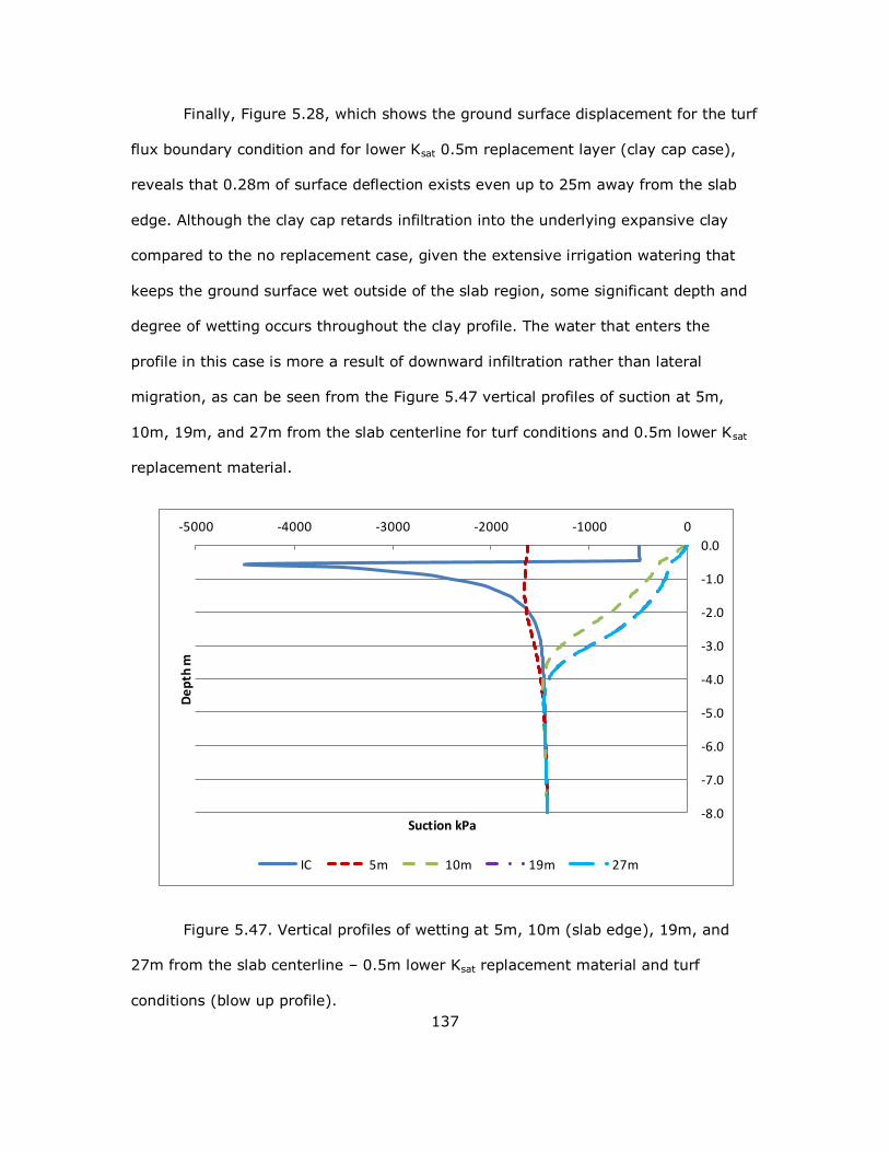
137
Finally, Figure 5.28, which shows the ground surface displacement for the turf
flux boundary condition and for lower Ksat 0.5m replacement layer (clay cap case),
reveals that 0.28m of surface deflection exists even up to 25m away from the slab
edge. Although the clay cap retards infiltration into the underlying expansive clay
compared to the no replacement case, given the extensive irrigation watering that
keeps the ground surface wet outside of the slab region, some significant depth and
degree of wetting occurs throughout the clay profile. The water that enters the
profile in this case is more a result of downward infiltration rather than lateral
migration, as can be seen from the Figure 5.47 vertical profiles of suction at 5m,
10m, 19m, and 27m from the slab centerline for turf conditions and 0.5m lower Ksat
replacement material.
Figure 5.47. Vertical profiles of wetting at 5m, 10m (slab edge), 19m, and
27m from the slab centerline – 0.5m lower Ksat replacement material and turf
conditions (blow up profile).
-8.0
-7.0
-6.0
-5.0
-4.0
-3.0
-2.0
-1.0
0.0
-5000 -4000 -3000 -2000 -1000 0
De
pth
m
Suction kPa
IC 5m 10m 19m 27m

138
5.9 Discussion
This study represents a unique investigation on the efficacy of remove and
replacement methods for mitigation of expansive soils in that the analyses are based
on fundamental unsaturated flow and stress-deformation principles. These analyses
provide a detailed look into the complexities of the mitigation mechanisms at play for
remove and replace options. The unsaturated flow/deformation analyses performed
show that the remove and replace technique can be very effective in mitigating both
total and differential deformation resulting from suction changes within expansive
soil profiles. However, the processes by which the remove and replace method
serves to mitigate expansive soil movements are complex and inter-related, and it is
clearly possible, based on findings from this study, for a user of this mitigation
method to select a remove and replace option that worsens the expansive soil
problem (e.g. high conductivity replacement soils can result in deep and high degree
of wetting). On the other hand, for many scenarios of removal and replacement and
surface flux conditions, the remove and replace method can be highly successful in
mitigating total and differential heave, which likely explains why this method has
been widely used in practice.
There are several aspects of the remove and replace method that must be
considered: (1) The effect of removal and replacement on depth and degree of
wetting within the soil profile, which is a function of both the replacement material
type and the depth (thickness) of the replacement layer. In addition, the
performance of the replacement material depends on the placement conditions
because placement moisture condition affects the conductivity of the layer. In the
end, depending on the replacement option selected, it is possible to increase or
decrease the depth and degree of wetting within the underlying clay profile. (2) To

139
the extent that the replacement soil is non-expansive (non-moisture sensitive or
“inert”) the remove and replace method gets rid of shrink/swell materials
immediately below the foundation. For a given depth and degree of wetting, removal
of expansive clay decreases total wetting-induced heave. In addition, because the
seat of movement is pushed deeper within the soil profile, differential heave is
reduced. However, the depth and degree of wetting cannot be guaranteed to
decrease (or even remain the same) when using the remove and replace method,
and thus the effect of the replacement of expansive soil with inert material has
highly variable impact on total and differential heave depending on the replacement
depth and replacement soil conductivity characteristics. Further, even if there is a
reduction in total and differential heave, the amount of reduction may not be
adequate to ensure good performance of the structure. (3) If the thickness of the
replacement layer is greater than the removed layer the confining pressure within
the underlying expansive soil layer will be increased, which decreases the swell
potential of clay. Although this is a known effect, this mechanism of increased
confinement was not studied in this research.
The impact of pushing the “seat” of wetting deeper into the soil reduces the
swelling feature on the surface (Walsh et.al, 2009). But the effect of remove and
replace mitigation on the depth, degree and rate of wetting is less clear. This study
sheds some light on the complexity of the unsaturated flow aspects of the remove
and replace mitigation technique. The complexities are primarily due to the highly
nonlinear nature of the unsaturated soil storage function (SWCC) and hydraulic
conductivity function. The hydraulic conductivity of an unsaturated soil varies over
several orders of magnitude, depending on the value of soil suction. Further, the
unsaturated hydraulic conductivity of granular soils can be lower than the

140
unsaturated hydraulic conductivity of a fine-grained soil, depending on the value of
soil suction. The net result is that the impact of various remove and replace options
is not always intuitive. Following are the key findings from this research study on
remove and replace mitigation wherein two very different surface flux conditions
were considered for various replacement depths and use of three differing hydraulic
conductivity function replacement materials were studied. The findings are based on
sound unsaturated soil principles incorporated into 2-D unsaturated flow and
unsaturated soil stress-deformation finite element code. Table 5.1 and Table 5.2
provide a summary of the various scenarios considered in this study. Table 5.1
includes the results obtained for the roof runoff surface flux condition and Table 5.2
includes the results obtained for the turf surface flux conditions.
Table 5.1. Heave reduction for different soil and depths of removal and
replacement for Roof Runoff Surface Flux Conditions
Replacement Soil
Type
Max .Depth of
Replacement m
Max. Total
Heave m
% Reduction
in Heave at
surface
(X=10m)
Differential
Heave
m
Lower Ksat 0.5 0.028 89 0.03
Same Ksat
0.75 0.063 75 0.01
2 0.058 77 ≈0
4 0.055 78 ≈0
Higher Ksat
0.75 0.195 22 0.1
2 0.165 34 0.01
4 0.153 39 ≈0
No Replacement - 0.25 - 0.23
The heave pattern obtained for turf flux conditions is different from the roof
runoff case. Unlike the roof runoff case the flux is evenly applied all over the top
exposed region of the profile. As a result of this the heave pattern is uniform below
and beyond the slab edge. However, the heave values are higher in turf as the final
suction values are much smaller in this as compared to the roof runoff. This is a

141
direct result of application of a surface flux condition consistent with poorly graded
surface conditions that do not provide for runoff of excess irrigation water. There is a
net wetting effect of the soil in this case. However, the removal and replacement
results follow the same trend in terms of reduction of wetting and reduction of heave
as for the roof runoff case. In all cases, removal and replacement of the upper
expansive soils shows a reduction in heave. However, it can be seen that there is
likely some optimal (i.e. most cost-effective) remove and replace option.
The 2m same Ksat replacement case works as well as the 0.5m cap to reduce
subsurface wetting and ground surface heave. The vertical heave reduction is only
slightly better in 2m same Ksat case. The initial and final suction and saturation
variation plot for 2m same Ksat shows the top region reaches to condition close to
saturation after 6 years.
A comparison between two replacement soils and depth for turf case is
presented in Table 5.2.
Table 5.2. Heave reduction for different soil and depths of removal and
replacement for Turf Surface Flux conditions.
Replacement
Soil Type
Max .Depth of
Replacement m
Max. Total
Heave at
surface m(X=10m)
Depth of
wetting%
Reduction in Heave at
surface
(X=10m)
Differential
heave
m
Lower Ksat 0.5 0.145 56 0.07
Same Ksat 2 0.119 64 ≈0
No Replacement - 0.33 - 0.32
There has to be a tradeoff between the depth up to which the seat of
movement is pushed down and depth of removal and replacement. For example,
when replacing the expansive soil with higher conductivity replacement soil a caution

142
should be exercised since the water tends to push down into the expansive clay
region due to its higher conductivity.
It can be observed that after a certain depth of removal there is no significant
decrease in the heave at the ground. Therefore it is very important to understand
that getting rid of the expansive soil in the entire depth of wetting might not be the
best solution economically. When removing the few upper meters of expansive soil
results are as effective in reducing heave as removing and replacing greater depths
with non-expansive soil, the opportunity for cost-saving/optimal design is available.
It is evident from the results of the cases analyzed in this study that pushing
the seat of wetting/movement deeper into the soil curbs the heave/shrinkage
movements and differential movements at the ground surface. The best choice
however, for replacement materials is expected to be site-specific, and dependent on
climatic and irrigation conditions, as a minimum.
Following is a brief summary of conclusions from this study:
1. The remove and replace option can be an effective technique for reducing
suction-change induced total and differential movements associated with
expansive soil profiles.
2. Placement of a low conductivity “clay cap” is effective in reducing the depth
and degree of wetting as well as total and differential movements resulting
from suction changes in expansive clay soils. The clay cap serves to retard
downward infiltration and upward evaporation from the soil profile, thus
reducing differential movements at the ground surface by providing for more
uniform subsurface moisture conditions. In this study the clay cap was
assumed to remain uncracked even during drying. Methods to minimize

143
cracking of a clay cap, such as covering with a relatively impermeable layer of
pavement, should be considered for field applications of the clay cap option.
While deeper layers of low conductivity clay would further reduce depth and
degree of moisture content change and serve to push the seat of movement
deeper within the soil profile, for practical applications there is a limit to the
thickness of clay replacement layer that can be used.
3. There is, conceptually, an optimal depth of removal and replacement that will
provide for acceptable total and differential movements. The optimal
thickness of replacement is a function of the surface flux boundary conditions
and the hydraulic conductivity characteristics and storage characteristics of
the replacement material. For example, when significant evaporation occurs
between wetting events, intermediate conductivity materials (such as silt and
low plasticity clays, perhaps) may provide a “sponge-type” effect wherein
water enters the replacement layer where it tends to be stored on top of the
higher conductivity expansive soil layer until an evaporation event removes
most of the applied water from the profile. If the removed layer thickness
becomes too great, however, infiltrating water may reach a depth such that
evaporation from the ground surface is not effective in removing the water –
so that the water continues into the underlying expansive clay over time.
4. In this study, as with actual field conditions, the expansion potential of the
expansive clay was reduced with depth as confinement due to overburden
pressures increased. In addition, presence of the replacement layer serves to
push the seat of movement deeper into the profile. However, if the underlying
clay layer is deep and deep wetting occurs, movements may still be
intolerable.

144
5. In this study it was shown that higher conductivity replacement layers result
in deeper wetting within the soil profile and therefore high conductivity
replacement soils, such as granular soils (sand cushions) are not a good
option, in general. In addition, higher conductivity replacement layer allow
greater lateral movement of water which can result in wetting of the
expansive clay and ground surface heave considerable distances away from
the source of wetting. The deeper wetting associated with lateral movement
of water also suggests that any sources of water that could move laterally
through the soil profile (either on-site or off-site) should be taken into
consideration in selection of the mitigation solution. In this study, the source
of wetting was restricted to downward infiltration only from on-site sources.
6. Given the tendency to compact replacement materials at or wet of optimum
(at relatively low suction values), the fact that hydraulic conductivity of soil
increases with decreasing suction must be considered in the evaluation of the
performance of a given replacement material type. For example, in this study
replacement material having the same saturated hydraulic conductivity as the
underlying expansive clay was found to have a sufficiently high hydraulic
conductivity at optimum moisture content placement conditions to allow
substantial lateral movement of water and rather deep wetting into the
underlying relatively dry expansive clay. This means that if a replacement soil
is placed very wet, it may, for certain surface flux conditions where
evaporation is minimal, perform similarly to a higher conductivity replacement
soil with regard to resulting depth, degree, and extent of wetting.
7. Given the complexities of the processes involved in remove and replace
mitigation solutions, it is difficult to intuitively know what is the optimal
solution for a given surface flux condition. Still, certain generalizations can be

145
made from the findings of this study. While it is difficult to know the optimal
replacement depth for any given surface flux or replacement layer thickness,
it is clear that extremely large replacement depths (e.g. the 4 m replacement
considered here) are unlikely to be optimal as one reaches a point of
diminishing return on total and differential ground surface movements. Also,
there are certain designs that are not expected to work well, such as use of
high conductivity replacement material type because of the tendency towards
deeper and greater degree of wetting when water enters the high conductivity
replacement material. The higher conductivity material placed on top of the
expansive clay can serve as a “bathtub” to collect water which then
penetrates to considerable depth within the underlying clay layer.

146
6 CONCLUSIONS AND FUTURE WORK
6.1 General
It has been long established that mitigation techniques are very important for
construction on expansive soils. The remove and replace technique is a very good
alternative when compared to other expensive mitigation methods. Although the
remove and replace option has been studied by several researchers in the past,
there is no comprehensive analytical study available to evaluate a reasonable
replacement material type and depth of removal and replacement when foundation is
constructed on expansive soil. The depth is removed and replaced either based on
past experience or some empirical data set. This study represents a unique
investigation on the efficacy of remove and replaces methods for mitigation of
expansive soils in that the analyses are based on fundamental unsaturated flow and
stress-deformation principles. These analyses provide a detailed look into the
complexities of the mitigation mechanisms at play for remove and replace options,
and demonstrate that the most appropriate and cost-effective depth of replacement
and replacement material type are not intuitively obvious. The results of this study
show that the remove and replace method can be highly successful in mitigating
total and differential heave, which likely explains why this method has been widely
used in practice. However, the processes involved are complex and inter-related,
resulting in the possibility of selection of a remove and replace option that worsens
the expansive soil problem (e.g. high conductivity replacement soils can result in
deep and high degree of wetting).

147
The study sets the stage for sound application of remove and replace
mitigation methods. However, in consideration of the complexities involved, and in
consideration of the wide-spread use of remove and replace methods in practice,
further study is warranted.
6.2 Recommendation for Future Work
This study provides a significant contribution to the understanding of remove
and replace methods for mitigation of moisture sensitive soil profiles such as
expansive clays and collapsible soil. However, there remain research questions that
should be addressed by future studies. Following is recommended for future work:
1. Longer simulations of remove and replace cases should be run in order to
assess the efficacy of removal depths and material under long term wetting.
2. Actual replacement soils and their volume change properties should be tested
in the laboratory and used in the unsaturated flow/deformation analyses. In
this study the replacement material properties were assumed such that the
replacement material had very low volume change in response to suction
changes.
3. Hypothetical cases were used in this study. To the extent possible, the
findings from this work should be validated for actual field case histories. This
is particularly important given the complex interactions at play in this
mitigation method.
4. The impact of distributed load on the slab should be studied to know how
much it helps to prevent heave, and the slab stiffness and soil-structure
interaction effects should be studied.

148
5. Three-dimensional volume change problems should be analyzed in future
when 3D modeling becomes less challenging.
6. Other surface flux boundary conditions should be studied, including in
particular, the study of turf conditions for a well-graded site where excess
irrigation water is run-off rather than allowed to infiltrate into the profile.

149
REFERENCES
Ahmed, A. 2009. Evaluation of Drying and Wetting Cycles with Soil Cushion to Mitigate the Potential of Expansive Soil in Upper Egypt. Department of Civil
Engineering, Beni-Suef University, Beni-Suef, Egypt
Bao, C. G., and Ng, C. W. W. 2000. Keynote lecture: Some thoughts and
studies on the prediction of slope stability in expansive soils. Proceedings of 2nd int. conf. on unsaturated soils and slope stability for expansive soils Vol (2):71-98.
Benson, C. H. and, Trast, J. M. 1995. Hydraulic Conductivity of Thirteen
Compacted Clays, STS Consultants Ltd., Clay and Clay Minerals Society Vol. 43,
no.6:669-681.
Bratton, Wesley L. Slab-On-Ground Foundations Constructed Over Expansive
Clay: Parameters to Predict Volume Change Potential by Dissertation In Civil
Engineering, Submitted to the Graduate Faculty of Texas Tech University. 1991
Burov, E. S. 1977. Using compensating cushions in the construction of structures on expansive soils. Proc., 1st National Symp. on Expansive Soils:166-169.
Harcourt-Butler Technological Institute, Kanpur, India.
California Building Standards and Codes for Residential Structures. 2010.
Celia, M. A., and Bouloutas, E. T. July 1990. A General Mass- Conservative
Numerical Solution for the Unsaturated Flow Equation. Water Resources Research Vol. 26(7):1483-1496.
Chen, F. H. 1988. Foundations on Expansive Soils, 2nd ed.: 463. Amsterdam:
Elsevier.
Chen, F. H. 1988. Foundations on Expansive Soils. Development in Geotechnical Engineering 54. Elsevier Science Publishers B. V.
Clemence, S. and Finbarr, A. 1981. Design Considerations for Collapsible
Soils. Journal of Geotechnical Engineering, ASCE 107(3): 305-318.
Coduto, P.D. 1999. Foundation Design – Principles and Practices. 54th edition. New Jersey: Prentice Hall.
Coppola, D. G. 2007. Introduction to International Disaster Management
Amsterdam: Elsevier Publication.

150
Day, R. W. June 2, 2006. Expansive Soils: Recent Advances in
Characterization and Treatment 1st edition, Taylor & Francis.
Dye, H. 2008. Moisture Movement through Expansive Soil and Impact on Performance of Residential Structures, PhD Dissertation, Arizona State University.
Dye, H.B., Houston, S.L., and Houston, W.N. July 2-4, 2008. Surface flux
boundary simplifications for flow through clay under landscaped conditions.
Unsaturated Soils: Advances in Geo-Engineering. Proceedings of the First European Conference on Unsaturated Soils, E-Unsat.: 805-810. Durham, UK. (ed. Toll, D.G.,
Augarde, C.E., Gallipoli, D. & Wheeler,S.J.), Leiden: CRC Press/Balkema.
Edlefsen , N. E., and Anderson, A. B. C. 1943. Thermodynamics of Soil
Moisture 15:31- 298. Hilgardi.
Fredlund, D. G, 2006. Unsaturated Soil Mechanics in Engineering Practice.
Journal of Geotechnical and Geotechnical Engineering 132(3):286-321.
Fredlund, D. G, Hung, Vu, Fredlund, M., and Thode, R. Oct 1st, 2004.
Modeling soil-structure interaction of slabs on expansive soils, Soilvision Systems Ltd.
Fredlund, D. G. 1979. Second Canadian Geotechnical Colloquium: Appropriate
Concepts and Technology for Unsaturated Soils. Canadian Geotechnical Journal
Vol.16, no.1:121-139.
Fredlund, D. G. May 18-19, 2000. Historical Developments and Milestones in unsaturated Soils, UNSAT ASIA, Keynote Address: 53-68. Singapore.
Fredlund, D. G., and Rahardjo, H. 1993. Soil Mechanics for Unsaturated soils.
New York:John Wiley & Sons.
Fredlund, D. G., and Rahardjo, H. 1994. Equations for the Soil-Water Characteristic Curve. Canadian Geotechnical Journal 31(3):521-532.
Fredlund, D. G. August 22-23, 1995. The Prediction of Heave in Expansive
Soils - Canada-Kenya Symposium on Unsaturated Soil Behaviour and Applications:
105-119. University of Nairobi, Nairobi, Kenya.
Fredlund, D. G., and Xing, A. 1994. Equations for the Soil Water
Characteristic Curve. Canadian Geotechnical Journal Vol.31:521-532.

151
Goode, J. C., Hamberg, D. J., and Nelson, J. D. 1984. Moisture Content and
Heave beneath Slabs on Grade. Fifth International Conference on Expansive Soils
1984:Preprints of Papers International Conference on Expansive Soils. Adelaide, S. Australia.
Hamberg, D. J. 1985. A Simplified Method for Predicting Heave in Expansive
Soils. M.Sc. thesis: 275, Colorado State Univ., Fort Collins.
Hamberg, D. J., and Nelson, J. D. 1984. Prediction of Floor Slab Heave. Proc. 5th Int. Conf. Expansive Soils: 137-140. Adelaide, Australia.
Hammel, J. E., Papendick, R. I., and Campbell, G. S. 1981. Fallow Tillage
Effects on Evaporation and Seedzone Water Content in a Dry Summer Climate. Soil
Science Society of America Journal 45:1016-1022.
Holland, J. E., and Richards, J. 1984. The Practical design of foundations for
light structures on expansive clays. Proceedings, 5th Int. Conf. on Expansive Soils,
ACT. Institution of Engineers, Australia.
Ho, D. Y. F., Fredlund, D. G., and Rahardjo, H. 1992. Volume Change Indices during loading and unloading of an unsaturated soil. Canadian Geotechnical Journal
Vol.29, No.2:195-207.
Holmes, R. M., 1961. Estimation of Soil Moisture Content Using Evaporation
Data. Proceedings of Hydrology Symposium, No. 2 Evaporation: 184-196. Ottawa:
Queen’s Printer.
Holtz, R. D., and Kovacs, W. D. 1981. An Introduction to Geotechnical
Engineering. Prentice-Hall, Inc.
Holtz, W. G., and Gibbs, G. J. 1956. Engineering Properties of Expansive
Clays. Trans. Am. Soc. Civ. Engrs. 121:641-677.
Holtz, W. G., and Hart, S. S. 1978. Home Construction On Shrinking And
Swelling Soils. American Society of Civil Engineers. Denver : Colorado Geological
Survey
Horton, R. E. 1940. An approach towards a physical interpretation of infiltration capacity, Soil Sci. Soc. Am.Proc. 5:399-417.
Houston, S. L. 1996. Foundations and pavements on unsaturated soils – Part
one: Collapsible soils. Proceedings of the 1st International Conference on Unsaturated
Soils, UNSAT ’95. 14211440. Paris, France.

152
Houston, S. L., Dye, H. B., Zapata, C. E., Walsh, K. D., and Houston, W. N.
February 1, 2011. Study of Expansive Soils and Residential Foundations on
Expansive Soils in Arizona. Journal of Performance of Constructed Facilities Vol. 25:No. 1.
Houston, S. L., Houston, W. N., Zapata, C. E., and Lawrence, C. 2001,
Geotechnical engineering practice for collapsible soils. Department of Civil and
Environmental Engineering, Arizona State University, Tempe, Arizona, 85287-5306.
Hung, Q. Vu, and Fredlund, D.G. 2000. Implementation of soil Property
Functions in Volume Change Analysis in Unsaturated Soils.
Hung, Q. Vu, and Fredlund, D.G. 2004. The prediction of one, two and three
dimensional heave in expansive soils, Canadian Geotechnical Journal Vol.41:713-737.
Hung, Q. Vu. Uncoupled and Coupled Solutions of Volume Change Problems in
Expansive Soils, Ph D. Dissertation: 319. Department of Civil Engineering, University
of Saskatchewan, Saskatoon, Saskatchewan, Canada.
International Building Code (IBC) 2006 & International Residential Code
(IRC), 2006.
Katti, R. K. 1979. Search for solutions to problems in black cotton soils. First
Indian Geotechnical Society Annual Lecture, Indian Geotechnical Journal 9-1:1–88.
Kerrane, J. P. What are Expansive Soils? Benson & Associates PC.
Komornick, A. K., and David D. 1969. Prediction of Swelling Pressure of Clays.
Proceedings ASCE, Journal of soil mechanics and Foundation Engineering Division
Vol.25, No. SM1:209-225. New York.
Komornik, A., Wiseman, G., and Ben-Yaacob, Y. 1969. Studies of In-Situ Moisture and Swelling Potential Profiles. Proc. 2nd Int. Conf. Unsaturated Expansive
Soils: 348-361. Texas.
Krohn, J. P., and Slosson, J. E. 1980. Assessment of Expansive Soils in the
United States. Proceedings of 4th International Conference on Expansive Soils:596-608. Denver, Colorado.
Lytton, R. 1994. Prediction of movement of expansive clay: Proceeding of
vertical and horizontal deformation of foundations and embankments. Geotechnical
Special Publication 2:1827–1845.

153
Lytton, R. L. 1977. Foundation on Expansive Soils. Desai, C. S., and Christian,
J. T. (Editors), Numerical Methods in Geotechnical Engineering: 427-458. New York:
McGraw-Hill.
Lytton, R. L. 1977. The Characterization of Expansive Soils in Engineering
Soils in Engineering, Presentation at the Symposium on Water Movement and
Equilibrum in Swelling Soils. American Geophysical Union. San Francisco, CA.
Lytton, R., Aubeny, C., and Bulut, R. 2004. Design procedures for pavements on expansive soils (Project Number 0-4518) Report 0-4518-1 Vol 1.
McKeen, R. G. 1992. A model for predicting expansive soil behavior.
Proceedings of the 7th International Conference on Expansive Soils: 1-6. Dallas,
Texas.
McKeen, R. G. 2001. Investigating field behavior of expansive clay soils.
Proc., Expansive Clay Soils and Vegetative Influence on Shallow Foundations, ASCE
82–94. Reston, VA.
McKeen, R. G., and Johnson, L. D. 1990. Climate-controlled soil design parameters for mat foundations. Journal of Geotechnical Engineering 116-7:1073–
1094.
McOmber, R. M., and Thompson R.W. 2000. Verification of Depth of Wetting
for Potential Heave Calculations. Advances in Unsaturated Geotechnics, ed.
Shackelford et al., ASCE Geotechnical Special Publication no. 99:409-422.
McWhorter, D. B, and Nelson, J. D, Nov. 1979. Unsaturated Flow Beneath
Tailings Impoundments, Journal of Geotechnical engineering Division, ASCE Vol
(105), No. GT11:1317-1334.
Murthy, V. R., and Praveen, G. V. 2008. Use of chemically stabilized soil as cushion material below light weight structures founded on expansive soil. Journal of
materials in civil and materials, ASCE 0899-1561(2008)20:5(392).
NAVFAC. 1971. Soil Mechanics, Foundation and Earth Structures, Design
Manual, NAVFACDM-7, Naval Facilities Engineering Command. Department of the Navy, Bureau of Yards and Docks, Washington, DC.
Nelson, J. D., Overton, D., and Durkee, D. B. 2001. Depth of wetting and
active zone. Proceedings of Geo-Institute Shallow Foundation and Soil Properties
Committee: 95-109.

154
Nelson, J. D. and Miller, D. J. 1992. Expansive Soils: Problems and Practice in
Foundation and Pavement Engineering. New York: John Wiley & Sons.
O'Neill, M. W., and Poormoayed, N. 1980. Methodology for foundations on expansive clays. ASCE Journal of Geotechnical Engineering Division: 1345-1364.
Richards, L. A. 1931. Capillary Conduction of Liquids through Porous Mediums
1:318-333. Physics, NY.
Rollins, K. and Rogers, G. W., 1994. Mitigation Measures for Small Structures on Collapsible Alluvial Soils, Journal Geotechnical Engineering, ASCE 120 (9).
Seed, H. B., Woodward, R. K., and Lundgren, R. 1962. Prediction if swelling
Potential for compacted Clays. Journal of Soil Mechanics division, ASCE Vol.88, SM3:
53-87.
Shackelford, C. D., Chiu, T. F., Young, R. N., and Thomas, H. R. 1997. The
influence of the capillary barrier effect on the use of sand under drains in waste
disposal practice. Geoenvironmental engineering, contaminated ground: Fate of
pollutants and remediation: 357-364. London: Thomas Telford.
SoilVision Systems Ltd. 2008. SVFlux & SVSolid User’s Manual. Saskatoon,
SK.
SoilVision Systems Ltd. 2009. SVOffice User’s Manual. Saskatoon, SK.
Thompson, R. W, 1997. Evaluation Protocol for Repair of Residences
Damaged by Expansive Soils. Proceedings of Sessions on Unsaturated Soils at Geo-Logan, The Geo-Institute, Special Publication No. 68, ASCE. Logan, Utah.
Vu, H. Q. 2000. Finite Element Method for The Prediction of Volume Change in
Expansive Soils. M.Sc. Thesis: 314. Department of Civil Engineering, University of
Saskatchewan, Saskatoon, Sask. Canada.
Walsh, K. D, Colby, C. A, Houston, W. N., and Houston, S. L. 2009. Method
for evaluation of depth of wetting in residential areas, Journal of Geotechnical and
Geoenvironmental Engineering Vol.135 (2):169-176.
Walsh, K. D, Houston, S. L., Houston, W. N., and Harraz, A. M. Nov, 2009. Finite Element Evaluation of Deep-Seated Swell. Proceedings of 4th Asia-Pacific
Conference on unsaturated Soils 23-25. Newcastle, Australia.
Warren, W. 1995. So your home is built on expansive soil. ASCE.

155
Wilson, G. W., Fredlund, D. G., and Barbour, S. L. 1994. Coupled Soil
Atmosphere Modeling For Soil Evaporation. Canadian Geotechnical Journal 31: 151-
161.
Wray, W. K, and Meyer, K. T. 2004. Expansive Clay Soil-A Widespread and
Costly Geohazard. Geo-Strata, ASCE Geo Institute 24-28.
www.azgs.az.gov/HomeOwners-OCR/HG4_problemsoils.pdf.
Zhan, L. T., and Ng, C. W. W. 2004. Analytical Analysis of Rainfall Infiltration Mechanism in Unsaturated Soils. International Journal of Geomechanics, ASCE. Vol.
4, No.4:273-284.

156
APPENDIX A
CONVERGENCE STUDY RESULTS

157
Table A1. Convergence study for the Initial trial Runs
Max Increment Grid size Avg. Dt Nodes Runtime (SV Flux)
0.5 Regrid 0.44045 520 1:54
0.5m 0.44669 2685 18:20
0.25m 0.41132 10545 58:47
0.1m 0.44668 62273 2:21:45
Max Increment Grid size Avg. Dt Nodes Runtime (SV Flux)
0.2 Regrid 0.17123 512 4:12
0.5m 0.17783 2685 21:14
0.25m 0.17783 10545 1:22:08
0.1m 0.17783 62273 3:45:12
Max Increment Grid size Avg. Dt Nodes Runtime (SV Flux)
0.1 Regrid 0.0895 550 20:41
0.5m 0.08887 2685 3:51:40
0.25m 0.08887 10545 8:55:36
0.1m 0.08887 62273 12:37:52
Max Increment Grid size Avg. Dt Nodes Runtime (SV Flux)
0.01 Regrid 0.00869 550 45:36
0.5m 0.00889 2685 6:57:30
0.25m 0.00889 10545 18:34:55
0.1m 0.00889 62273 25:34:45
0.001 Regrid 0.00869 550 8:45:37
0.5m 0.00889 2685 38:47:50
0.25m 0.00889 10545 55:30:16
0.1m 0.00889 62273 -

158
A.1 Suction Results for Different Δx and Constant Δt (Initial
Preliminary/Trial Runs)
Figure A.1. Suction variation below slab edge (X=10m) for Δt=0.01
Figure A.2. Suction variation below slab edge (X=10m) for Δt=0.1

159
Figure A.3. Suction variation below slab edge (X=10m) for Δt=0.2
Figure A.4. Suction variation below slab edge (X=10m) for Δt=0.5

160
A.2 Suction Results Different Δt and Constant Δx (Initial Trial Runs)
Figure A.5. Suction variation below slab edge (X=10m) for Regrid
Figure A.6. Suction variation below slab edge (X=10m) for Δx = 0.5m

161
Figure A.7. Suction variation below slab edge (X=10m) for Δx = 0.25m
Figure A.8. Suction variation below slab edge (X=10m) for Δx = 0.1m

162
A.3 Saturation Results for Different Δx and Constant Δt (Initial Trial Runs)
Figure A.9.Saturation variation below slab edge (X=10m) for Δt = 0.01m
Figure A.10. Saturation variation below slab edge (X=10m) for Δt = 0.1m
-8
-7
-6
-5
-4
-3
-2
-1
0
0 0.2 0.4 0.6 0.8 1
Dep
th b
elow
sla
b ed
ge m
Saturation
regrid 0.5m 0.25m 0.1m
-8
-7
-6
-5
-4
-3
-2
-1
0
0 0.2 0.4 0.6 0.8 1
De
pth
be
low
sla
b e
dge
m
Saturation
regrid 0.5m 0.25m 0.1m

163
Figure A.11. Saturation variation below slab edge (X=10m) for Δt = 0.2m
Figure A.12. Saturation variation below slab edge (X=10m) for Δt = 0.5m
-8
-7
-6
-5
-4
-3
-2
-1
0
0 0.2 0.4 0.6 0.8 1
De
pth
be
low
sla
b e
dge
m
Saturation
regrid 0.5m 0.25m 0.1m
- 8
- 7
- 6
- 5
- 4
- 3
- 2
- 1
0
0 0.2 0.4 0.6 0.8 1
Saturation
regrid 0.5m 0.25m

164
A.4 Saturation Results for Different Δt and Constant Δx (Initial Trial Runs)
Figure A.13. Saturation variation below slab edge (X=10m) for Regrid
Figure A.14. Saturation variation below slab edge (X=10m) for Δx = 0.5m
-8
-7
-6
-5
-4
-3
-2
-1
0
0 0.2 0.4 0.6 0.8 1
De
pth
be
low
sla
b e
dge
m
Degree of saturation
dt=0.1 dt=0.2 dt=0.5 dt=0.01
-8
-7
-6
-5
-4
-3
-2
-1
0
0 0.2 0.4 0.6 0.8 1
Dep
th b
elow
sla
b ed
ge m
Degree of saturation
dt=0.1 dt=0.2 dt=0.5 dt=0.01

165
Figure A.15. Saturation variation below slab edge (X=10m) for Δx = 0.25m
Figure A.16. Saturation variation below slab edge (X=10m) for Δx = 0.1m
-8
-7
-6
-5
-4
-3
-2
-1
0
0 0.2 0.4 0.6 0.8 1
Dep
th b
elow
sla
b ed
ge m
Degree of saturation
dt=0.1 dt=0.2 dt=0.5 dt=0.01
-8
-7
-6
-5
-4
-3
-2
-1
0
0 0.2 0.4 0.6 0.8 1
De
pth
be
low
sla
b e
dge
m
Degree of saturation
dt=0.1 dt=0.2 dt=0.5 dt=0.01

166
APPENDIX B
5TH YR CLIMATIC CONDITIONS RESULTS

167
B.1 5 Yr Climatic Condition Runs for Intact Soil (Initial Condition for Final
Remove and Replacement SV Flux Runs)
Figure B.1. Section below slab edge
Figure B.2. Vertical profile below slab edge (see Figure B.1)

168
Figure B.3. Horizontal section at the ground surface
Figure B.4. History pwp plot at the ground surface (see Figure B.3)

169
Figure B.5. History pwp plot at the Y=0.25m below surface
Figure B.6. History pwp plot at the Y= 0.5m below surface

170
Figure B.7. History pwp plot at Y = 1m below ground surface
Figure B.8. History pwp plot at Y = 1.5m below ground surface

171
Figure B.9. History pwp plot at Y= 2m below ground surface

172
APPENDIX C
IC AND FC SUCTION PROFILES FOR DIFFERENT DISTANCES FROM SLAB CENTERLINE

173
C.1 Roof Runoff Boundary Conditions Case
The suction plots included in this section are for the vertical sections of the
soil profile as shown in the sketch below. The plots shown below are for all the
replacement cases and no replacement case.
0m 5m 8m
11m 19m 27m 35m
1m 8m 8m 8m
9m 10m

174
C.1.1 IC and FC Suction Plots for No Replacement Expansive Clay Case
Figure C.1. - Vertical suction profile at 0m
Figure C.2. Vertical suction profile at 5m
-30
-25
-20
-15
-10
-5
0
-60000 -50000 -40000 -30000 -20000 -10000 0D
ep
th m
Suction kPa
IC FC
-30
-25
-20
-15
-10
-5
0
-60000 -50000 -40000 -30000 -20000 -10000 0
De
pth
m
Suction kPa
IC FC

175
Figure C.3. Vertical suction profile at 8m
Figure C.4. Vertical suction profile at 9m
-30
-25
-20
-15
-10
-5
0
-60000 -50000 -40000 -30000 -20000 -10000 0
De
pth
m
Suction kPa
IC FC
-30
-25
-20
-15
-10
-5
0
-60000 -50000 -40000 -30000 -20000 -10000 0
De
pth
m
Suction kPa
IC FC

176
Figure C.5. Vertical suction profile at 10m
Figure C.6. Vertical suction profile at 11m
-30
-25
-20
-15
-10
-5
0
-60000 -50000 -40000 -30000 -20000 -10000 0
De
pth
m
Suction kPa
IC FC
-30
-25
-20
-15
-10
-5
0
-60000 -50000 -40000 -30000 -20000 -10000 0
De
pth
m
Suction kPa
IC FC

177
Figure C.7. Vertical suction profile at 19m
Figure C.8. Vertical suction profile at 27m
-30
-25
-20
-15
-10
-5
0
-60000 -50000 -40000 -30000 -20000 -10000 0
De
pth
m
Suction kPa
IC FC
-30
-25
-20
-15
-10
-5
0
-60000 -50000 -40000 -30000 -20000 -10000 0
De
pth
m
Suction kPa
IC FC

178
Figure C.9. Vertical suction profile at 35m
C.1.2 IC and FC Suction Plots for 0.5m Lower Ksat Replacement Layer Case
Figure C.10. Vertical suction profile at 0m
-30
-25
-20
-15
-10
-5
0
-60000 -50000 -40000 -30000 -20000 -10000 0
De
pth
m
Suction kPa
IC FC
-30.0
-25.0
-20.0
-15.0
-10.0
-5.0
0.0
-5000 -4000 -3000 -2000 -1000 0
De
pth
m
Suction kPa
IC FC

179
Figure C.11. Vertical suction profile at 5m
Figure C.12. Vertical suction profile at 8m
-30.0
-25.0
-20.0
-15.0
-10.0
-5.0
0.0
-5000 -4000 -3000 -2000 -1000 0
De
pth
m
Suction kPa
IC FC
-30.0
-25.0
-20.0
-15.0
-10.0
-5.0
0.0
-5000 -4000 -3000 -2000 -1000 0
De
pth
m
Suction kPa
IC FC

180
Figure C.13. Vertical suction profile at 9m
Figure C.14. Vertical suction profile at 10m
-30.0
-25.0
-20.0
-15.0
-10.0
-5.0
0.0
-5000 -4000 -3000 -2000 -1000 0
De
pth
m
Suction kPa
IC FC
-30.0
-25.0
-20.0
-15.0
-10.0
-5.0
0.0
-5000 -4000 -3000 -2000 -1000 0
De
pth
m
Suction kPa
IC FC

181
Figure C.15. Vertical suction profile at 11m
Figure C.16. Vertical suction profile at 19m
-30.0
-25.0
-20.0
-15.0
-10.0
-5.0
0.0
-5000 -4000 -3000 -2000 -1000 0
De
pth
m
Suction kPa
IC FC
-30.0
-25.0
-20.0
-15.0
-10.0
-5.0
0.0
-5000 -4000 -3000 -2000 -1000 0
De
pth
m
Suction kPa
IC FC

182
Figure C.17. Vertical suction profile at 27m
Figure C.18. Vertical suction profile at 35m
-30.0
-25.0
-20.0
-15.0
-10.0
-5.0
0.0
-5000 -4000 -3000 -2000 -1000 0
De
pth
m
Suction kPa
IC FC
-30.0
-25.0
-20.0
-15.0
-10.0
-5.0
0.0
-5000 -4000 -3000 -2000 -1000 0
De
pth
m
Suction kPa
IC FC

183
C.1.3 IC and FC Suction Plots for 0.75m Same Ksat Replacement Case
Figure C.19. Vertical suction profile at 0m section
Figure C.20. Vertical suction profile at 5m section
-30
-25
-20
-15
-10
-5
0
-3500 -3000 -2500 -2000 -1500 -1000 -500 0
De
pth
m
Suction kPa
IC FC
-30.00
-25.00
-20.00
-15.00
-10.00
-5.00
0.00
-3500 -3000 -2500 -2000 -1500 -1000 -500 0
De
pth
m
Suction kPa
IC FC

184
Figure C.21. Vertical suction profile at 8m section
Figure C.22. Vertical suction profile at 9m section
-30.00
-25.00
-20.00
-15.00
-10.00
-5.00
0.00
-3500 -3000 -2500 -2000 -1500 -1000 -500 0
De
pth
m
Suction kPa
-30.00
-25.00
-20.00
-15.00
-10.00
-5.00
0.00
-3500 -3000 -2500 -2000 -1500 -1000 -500 0
De
pth
m
Suction kPa
-IC --- FC

185
Figure C.23. Vertical suction profile at 10m section
Figure C.24. Vertical suction profile at 11m section
-30.00
-25.00
-20.00
-15.00
-10.00
-5.00
0.00
-3500 -3000 -2500 -2000 -1500 -1000 -500 0
De
pth
m
pwp kPa
IC FC
-30.00
-25.00
-20.00
-15.00
-10.00
-5.00
0.00
-5000 -4000 -3000 -2000 -1000 0
De
pth
m
Suction kPa
IC FC

186
Figure C.25. Vertical suction profile at 19m section
Figure C.26. Vertical suction profile at 27m section
-30.00
-25.00
-20.00
-15.00
-10.00
-5.00
0.00
-5000 -4000 -3000 -2000 -1000 0
De
pth
m
SuctionkPa
IC FC
-30.00
-25.00
-20.00
-15.00
-10.00
-5.00
0.00
-5000 -4000 -3000 -2000 -1000 0
De
pth
m
Suction kPa
IC FC

187
Figure C.27. Vertical suction profile at 35m section
C.1.4 IC and FC Suction Plots for 2m Same Ksat Replacement Layer Case
Figure C.28. Vertical suction profile at 0m
-30.00
-25.00
-20.00
-15.00
-10.00
-5.00
0.00
-5000 -4000 -3000 -2000 -1000 0
De
pth
m
Suction kPa kPa
IC FC
-30
-25
-20
-15
-10
-5
0
-2000 -1500 -1000 -500 0
De
pth
m
Suction kPa
IC FC

188
Figure C.29. Vertical suction profile at 5m
Figure C.30. Vertical suction profile at 8m
-30
-25
-20
-15
-10
-5
0
-2000 -1500 -1000 -500 0
De
pth
m
Suction kPa
IC FC
-30
-25
-20
-15
-10
-5
0
-2000 -1500 -1000 -500 0
De
pth
m
Suction kPa
IC FC

189
Figure C.31. Vertical suction profile at 9m
Figure C.32. Vertical suction profile at 10m
-30
-25
-20
-15
-10
-5
0
-2000 -1500 -1000 -500 0
De
pth
m
Suction kPa
IC FC
-30.00
-25.00
-20.00
-15.00
-10.00
-5.00
0.00
-2500 -2000 -1500 -1000 -500 0
De
pth
m
Suction kPa
IC FC

190
Figure C.33. Vertical suction profile at 11m
Figure C.34. Vertical suction profile at 19m
-30
-25
-20
-15
-10
-5
0
-5000 -4000 -3000 -2000 -1000 0
De
pth
m
Suction kPa
IC FC
-30
-25
-20
-15
-10
-5
0
-4000 -3500 -3000 -2500 -2000 -1500 -1000 -500 0
De
pth
m
Suction kPa
IC FC

191
Figure C.35. Vertical suction profile at 27m
Figure C.36. Vertical suction profile at 35m
-30
-25
-20
-15
-10
-5
0
-4000 -3500 -3000 -2500 -2000 -1500 -1000 -500 0
De
pth
m
Suction kPa
IC FC
-30
-25
-20
-15
-10
-5
0
-4000 -3500 -3000 -2500 -2000 -1500 -1000 -500 0
De
pth
m
Suction kPa
IC FC

192
C.1.5 IC and FC Suction Plots for 4m Same Ksat Replacement Layer Case
Figure C.37. Vertical suction profile at 0m
Figure C.38. Vertical suction profile at 5m
-30
-25
-20
-15
-10
-5
0
-2000 -1500 -1000 -500 0
De
pth
m
Suction kPa
IC FC
-30.00
-25.00
-20.00
-15.00
-10.00
-5.00
0.00
-2000 -1500 -1000 -500 0
De
pth
m
Suction kPa
IC FC

193
Figure C.39. Vertical suction profile at 8m
Figure C.40. Vertical suction profile at 9m
-30.00
-25.00
-20.00
-15.00
-10.00
-5.00
0.00
-2000 -1500 -1000 -500 0
De
pth
m
Suction kPa
IC FC
-30.00
-25.00
-20.00
-15.00
-10.00
-5.00
0.00
-2000 -1500 -1000 -500 0
De
pth
m
Suction kPa
IC FC

194
Figure C.41. Vertical suction profile at 10m
Figure C.42. Vertical suction profile at 11m
-30.00
-25.00
-20.00
-15.00
-10.00
-5.00
0.00
-2000 -1500 -1000 -500 0
De
pth
m
Suction kPa
IC FC
-30.00
-25.00
-20.00
-15.00
-10.00
-5.00
0.00
-5000 -4000 -3000 -2000 -1000 0
De
pth
m
Suction kPa
IC FC

195
Figure C.43. Vertical suction profile at 19m
Figure C.44. Vertical suction profile at 27m
-30.00
-25.00
-20.00
-15.00
-10.00
-5.00
0.00
-4000 -3500 -3000 -2500 -2000 -1500 -1000 -500 0
De
pth
m
Suction kPa
IC FC
-30.00
-25.00
-20.00
-15.00
-10.00
-5.00
0.00
-4000 -3500 -3000 -2500 -2000 -1500 -1000 -500 0
De
pth
m
Suction kPa
IC FC

196
Figure C.45. Vertical suction profile at 35m
E.1.6 IC and FC Suction Plots for 0.75m Higher Ksat Replacement Case
Figure C.46. Vertical suction profile at 0m
-30.00
-25.00
-20.00
-15.00
-10.00
-5.00
0.00
-4000 -3500 -3000 -2500 -2000 -1500 -1000 -500 0
De
pth
m
Suction kPa
IC FC
-30
-25
-20
-15
-10
-5
0
-3500 -3000 -2500 -2000 -1500 -1000 -500 0
De
pth
m
Suction kPa
IC FC

197
Figure C.47. Vertical suction profile at 5m
Figure C.48. Vertical suction profile at 8m
-30
-25
-20
-15
-10
-5
0
-3500 -3000 -2500 -2000 -1500 -1000 -500 0
De
pth
m
Suction kPa
IC FC
-30
-25
-20
-15
-10
-5
0
-3500 -3000 -2500 -2000 -1500 -1000 -500 0
De
pth
m
Suction kPa
IC FC

198
Figure C.49.Vertical suction profile at 9m
Figure C.50. Vertical suction profile at 10m
-30
-25
-20
-15
-10
-5
0
-3500 -3000 -2500 -2000 -1500 -1000 -500 0
De
pth
m
Suction kPa
IC FC
-30.00
-25.00
-20.00
-15.00
-10.00
-5.00
0.00
-3500 -3000 -2500 -2000 -1500 -1000 -500 0
De
pth
m
Suction kPa
IC FC

199
Figure C.51. Vertical suction profile at 11m
Figure C.52. Vertical suction profile at 19m
-30
-25
-20
-15
-10
-5
0
-3500 -3000 -2500 -2000 -1500 -1000 -500 0
De
pth
m
Suction kPa
IC FC
-30
-25
-20
-15
-10
-5
0
-3500 -3000 -2500 -2000 -1500 -1000 -500 0
De
pth
m
Suction kPa
IC FC

200
Figure C.53. Vertical suction profile at 27m
Figure C.54. Vertical suction profile at 35m
-30
-25
-20
-15
-10
-5
0
-3500 -3000 -2500 -2000 -1500 -1000 -500 0
De
pth
m
Suction kPa
IC FC
-30
-25
-20
-15
-10
-5
0
-3500 -3000 -2500 -2000 -1500 -1000 -500 0
De
pth
m
Suction kPa
IC FC

201
C.1.7 IC and FC Suction Plots for 2m Higher Ksat Replacement Case
Figure C.55. Vertical suction profile at 0m
Figure C.56. Vertical suction profile at 5m
-30
-25
-20
-15
-10
-5
0
-2000 -1500 -1000 -500 0
De
pth
m
Suction kPa
IC FC
-30
-25
-20
-15
-10
-5
0
-2000 -1500 -1000 -500 0
De
pth
m
Suction kPa
IC FC

202
Figure C.57. Vertical suction profile at 8m
Figure C.58. Vertical suction profile at 9m
-30
-25
-20
-15
-10
-5
0
-2000 -1500 -1000 -500 0
De
pth
m
Suction kPa
IC FC
-30
-25
-20
-15
-10
-5
0
-2000 -1500 -1000 -500 0
De
pth
m
Suction kPa
IC FC

203
Figure C.59. Vertical suction profile at 10m
Figure C.60. Vertical suction profile at 11m
-30.00
-25.00
-20.00
-15.00
-10.00
-5.00
0.00
-2000 -1500 -1000 -500 0
De
pth
m
Suctionn kPa
IC FC
-30
-25
-20
-15
-10
-5
0
-2000 -1500 -1000 -500 0
De
pth
m
Suction kPa
IC FC

204
Figure C.61. Vertical suction profile at 19m
Figure C.62. Vertical suction profile at 27m
-30
-25
-20
-15
-10
-5
0
-2500 -2000 -1500 -1000 -500 0
De
pth
m
Suction kPa
IC FC
-30
-25
-20
-15
-10
-5
0
-2500 -2000 -1500 -1000 -500 0
De
pth
m
Suction kPa
IC FC

205
Figure C.63. Vertical suction profile at 35m
C.1.8 IC and FC Suction Plots for 4m higher Ksat Replacement Layer Case
Figure C.64. Vertical suction profile at 0m
-30
-25
-20
-15
-10
-5
0
-2500 -2000 -1500 -1000 -500 0
De
pth
m
Suction kPa
IC FC
-30.0
-25.0
-20.0
-15.0
-10.0
-5.0
0.0
-2000 -1500 -1000 -500 0
De
pth
m
Suction kPa
IC FC

206
Figure C.65. Vertical suction profile at 5m
Figure C.66. Vertical suction profile at 8m
-30.0
-25.0
-20.0
-15.0
-10.0
-5.0
0.0
-2000 -1500 -1000 -500 0
De
pth
m
Suction kPa
IC FC
-30.00
-25.00
-20.00
-15.00
-10.00
-5.00
0.00
-2000 -1500 -1000 -500 0
De
pth
m
Suction kPa
IC FC

207
Figure C.67. Vertical suction profile at 9m
Figure C.68. Vertical suction profile at 10m
-30.0
-25.0
-20.0
-15.0
-10.0
-5.0
0.0
-2000 -1500 -1000 -500 0
De
pth
m
Suction kPa
IC FC
-30.00
-25.00
-20.00
-15.00
-10.00
-5.00
0.00
-2000 -1500 -1000 -500 0
De
pth
m
Suction kPa
IC FC

208
Figure C.69. Vertical suction profile at 11m
Figure C.70. Vertical suction profile at 19m
-30.0
-25.0
-20.0
-15.0
-10.0
-5.0
0.0
-2000 -1500 -1000 -500 0
De
pth
m
Suction kPa
IC FC
-30.0
-25.0
-20.0
-15.0
-10.0
-5.0
0.0
-2500 -2000 -1500 -1000 -500 0
De
pth
m
Suction kPa
IC FC

209
Figure C.71. Vertical suction profile at 27m
Figure C.72. Vertical suction profile at 35m
-30.0
-25.0
-20.0
-15.0
-10.0
-5.0
0.0
-2500 -2000 -1500 -1000 -500 0
De
pth
m
Suction kPa
IC FC
-30.0
-25.0
-20.0
-15.0
-10.0
-5.0
0.0
-2500 -2000 -1500 -1000 -500 0
De
pth
m
Suction kPa
IC FC

210
C.2 Turf Landscape Boundary Conditions Case
The suction plots included in this section are for the vertical sections of the
soil profile as shown in the sketch below. The plots shown below are for all the
replacement cases and no replacement case.
5m
8m
11m 19m 27m 35m
9m 10m
0m
1m 8m 8m 8m

211
C.2.1 IC and FC PWP Plots for No Replacement Expansive Clay Case
Figure C.73. Vertical suction profile at 0m
Figure C.74. Vertical suction profile at 5m
-30
-25
-20
-15
-10
-5
0
-60000 -50000 -40000 -30000 -20000 -10000 0
De
pth
m
Suction kPa
IC FC
-30
-25
-20
-15
-10
-5
0
-60000 -50000 -40000 -30000 -20000 -10000 0
De
pth
m
Suction kPa
IC FC

212
Figure C.75. Vertical suction profile at 8m
Figure C.76. Vertical suction profile at 9m
-30
-25
-20
-15
-10
-5
0
-60000 -50000 -40000 -30000 -20000 -10000 0
De
pth
m
Suction kPa
IC FC
-30
-25
-20
-15
-10
-5
0
-60000 -50000 -40000 -30000 -20000 -10000 0
De
pth
m
Suction kPa
IC FC

213
Figure C.77.Vertical suction profile at 10m
Figure C.78. Vertical suction profile at 11m
-30.00
-25.00
-20.00
-15.00
-10.00
-5.00
0.00
-60000 -50000 -40000 -30000 -20000 -10000 0
De
pth
m
Suction kPa
IC FC
-30
-25
-20
-15
-10
-5
0
-60000 -50000 -40000 -30000 -20000 -10000 0
De
pth
m
Suction kPa
IC FC

214
Figure C.79. Vertical suction profile at 19m
Figure C.80. Vertical suction profile at 27m
-30
-25
-20
-15
-10
-5
0
-60000 -50000 -40000 -30000 -20000 -10000 0
De
pth
m
Suction Kpa
IC FC
-30
-25
-20
-15
-10
-5
0
-60000 -50000 -40000 -30000 -20000 -10000 0
De
pth
m
Suction kPa
IC FC

215
Figure C.81. Vertical suction profile at 35m
C.2.2 IC and FC Suction Plots 0.5m Lower Ksat Replacement Layer Case
Figure C.82. Vertical suction profile at 0m
-30
-25
-20
-15
-10
-5
0
-60000 -50000 -40000 -30000 -20000 -10000 0
De
pth
m
Suction kPa
IC FC
-30.0
-25.0
-20.0
-15.0
-10.0
-5.0
0.0
-5000 -4000 -3000 -2000 -1000 0
De
pth
m
Suction kPa
IC FC

216
Figure C.83. Vertical suction profile at 5m
Figure C.84. Vertical suction profile at 8m
-30.0
-25.0
-20.0
-15.0
-10.0
-5.0
0.0
-5000 -4000 -3000 -2000 -1000 0
De
pth
m
Suction Kpa
IC FC
-30.0
-25.0
-20.0
-15.0
-10.0
-5.0
0.0
-5000 -4000 -3000 -2000 -1000 0
De
pth
m
Suction kPa
IC FC

217
Figure C.85. Vertical suction profile at 9m
Figure C.86. Vertical suction profile at 10m
-30.0
-25.0
-20.0
-15.0
-10.0
-5.0
0.0
-5000 -4000 -3000 -2000 -1000 0
De
pth
m
Suction kPa
IC FC
-30.00
-25.00
-20.00
-15.00
-10.00
-5.00
0.00
-5000 -4000 -3000 -2000 -1000 0
De
pth
m
Suction kPa
IC FC

218
Figure C.87. Vertical suction profile at 11m
Figure C.88. Vertical suction profile at 19m
-30.0
-25.0
-20.0
-15.0
-10.0
-5.0
0.0
-5000 -4000 -3000 -2000 -1000 0
De
pth
m
Suction kPa
IC FC
-30.0
-25.0
-20.0
-15.0
-10.0
-5.0
0.0
-5000 -4000 -3000 -2000 -1000 0
De
pth
m
Suction kPa
IC FC

219
Figure C.89. Vertical suction profile at 27m
Figure C.90. Vertical suction profile at 35m
-30.0
-25.0
-20.0
-15.0
-10.0
-5.0
0.0
-4000 -3500 -3000 -2500 -2000 -1500 -1000 -500 0
De
pth
m
Suction kPa
IC FC
-30.0
-25.0
-20.0
-15.0
-10.0
-5.0
0.0
-5000 -4000 -3000 -2000 -1000 0
De
pth
m
Suction kPa
IC FC

220
C.2.3 IC and FC Suction Plots 2m Same Ksat Replacement Layer Case
Figure C.91. Vertical suction profile at 0m
Figure C.92. Vertical suction profile at 5m
-30
-25
-20
-15
-10
-5
0
-2000 -1500 -1000 -500 0
De
pth
m
Suction kPa
IC FC
-30
-25
-20
-15
-10
-5
0
-2000 -1500 -1000 -500 0
De
pth
m
Suction kPa
IC FC

221
Figure C.93. Vertical suction profile at 8m
Figure C.94. Vertical suction profile at 9m
-30
-25
-20
-15
-10
-5
0
-2000 -1500 -1000 -500 0
De
pth
m
Suction kPa
IC FC
-30
-25
-20
-15
-10
-5
0
-2000 -1500 -1000 -500 0
De
pth
m
SuctionkPa
IC FC

222
Figure C.95. Vertical suction profile at 10m
Figure C.96. Vertical suction profile at 11m
-30.00
-25.00
-20.00
-15.00
-10.00
-5.00
0.00
-2000 -1500 -1000 -500 0
De
pth
m
Suction kPa
IC FC
-30
-25
-20
-15
-10
-5
0
-2000 -1500 -1000 -500 0
De
pth
m
Suction kPa
IC FC

223
Figure C.97. Vertical suction profile at 19m
Figure C.98. Vertical suction profile at 27m
-30
-25
-20
-15
-10
-5
0
-2000 -1500 -1000 -500 0
De
pth
m
Suction kPa
IC FC
-30
-25
-20
-15
-10
-5
0
-2000 -1500 -1000 -500 0
De
pth
m
Suction kPa
IC FC

224
Figure C.99. Vertical suction profile at 35m
-30
-25
-20
-15
-10
-5
0
-2000 -1500 -1000 -500 0
De
pth
m
Suction kPa
IC FC

225
APPENDIX D
1ST PANAM CONFERENCE: EFFECT OF SOIL REPLACEMENT OPTION ON SURFACE DEFLECTIONS FOR EXPANSIVE CLAY PROFILES

226
INTRODUCTION Expansive soils are associated with shrink and swell behavior and may cause serious damage to structures. Residential foundations such as slab-on ground are generally built on unsaturated soils including expansive soils and are subject to deformations associated with changes in matric suction/ moisture content in the soil. The problem of expansive soils is more pronounced in arid regions where changes in soil suction as a result of development can be much greater than in humid regions. Expansive soils are also called moisture sensitive soils because when subjected to wetting, they undergo substantial volume changes associated with the swelling process. Various methods are available and practiced to reduce swelling in soils at the ground surface to prevent the damage caused to structures. Mitigation measures may be broadly defined as any actions or designs that lessen or solve moisture sensitive soil problems (Houston et al. 2001). Among the various techniques for expansive soil
mitigation, the removal and replacement technique
(remove-and-replace) is very popular for lightly
loaded structures and shallow foundations. The
heave reducing effect of replacement of expansive
soil with a non expansive layer has been studied by
various authors (Katti 1979, Walsh et al 2009,
Murthy & Praveen 2008) in the past. A large volume
of intact soil when replaced with non expansive soil
can attenuate the surface heave feature. The
mechanisms for reduction of heave are: (1) removal
of expansive soil with non-expansive soil results in a
zone of no-heave where the expansive soils are
replaced, thereby reducing surface heave, (2) the
replacement soil may change the degree and depth
of wetting in the native expansive clay profile by
increasing, decreasing, or having only minimal
effect on the amount of surface and near-surface
water that infiltrates into the soil, (3) the placement
of a non-expansive soil layer pushes the seat of
movement deeper into the profile, thereby reducing
the differential movements at the ground surface,
and (4) the non-expansive soil layer may provide
Effect of Soil Replacement Option on Surface Deflections for Expansive Clay Profiles
A. Bharadwaj, S.L. Houston, W.N. Houston & B. Welfert Arizona State University, Tempe, AZ, USA
K.D. Walsh San Diego State University, San Diego, CA, USA
ABSTRACT: In this paper the results of a stress-deformation parametric analysis are presented to show the effect of an artificial non-expansive replacement layer over an intact expansive soil on the heave at the surface. Finite element code SV Flux and SV Solid are used to perform the stress-deformation analysis. Climatic boundary conditions for a semi arid region are used. Significant decreases in the heave amount were noted, depending on the thickness and soil type of the replacement soil.

227
increased confinement for any expansive soil that
does get wet, thereby reducing volume change
In general, the non-expansive soil layer could have a
saturated hydraulic conductivity the same as, higher
than, or lower than the underlying expansive soil. As
a part of an on-going study at Arizona State
University, the full range of hydraulic properties of
the replacement layer is being evaluated. In this
paper, preliminary findings are presented for the
case of remove-and-replace mitigation where the
replacement layer has a higher hydraulic
conductivity than the underlying clay. This
represents, for example replacement of expansive
soil with a non-expansive granular fill.
ANALYSIS OF SLAB-ON-GROUND FOUNDATION ON EXPANSIVE CLAY PROFILE WITH REMOVE-AND-REPLACEMENT MITIGATION The problem that was analyzed is described schematically in figure 1. In these analyses the problem is analyzed as a two-dimensional (2D) problem for both fluid flow and deformation. The soil properties of clay typical of highly plastic clays in the Phoenix, Arizona, region were used. The clay is classified as CH, has a LL of 85 and a PI of 53 and a swell pressure of 700 kPa. The basic soil properties of the expansive clay are tabulated below in Table 1. In the simulation performed, roof runoff from the residential house falls directly on the edge of the foundation of the house. A pond of 150mm (6 inches) depth is allowed to occur a during rain event, and any additional roof runoff is allowed to run off of the site. The surface flux conditions outside of the region of ponding correspond to natural climatic conditions. The surface flux simulates desert landscaping conditions with some degree of ponding of rain water next to the structure. This has been observed to be a fairly common condition for residential structures in the Phoenix, AZ area (Dye 2008). The concentration of water next to the structure can cause differential heave which can damage the structure. The position of the domain boundaries (depth and width of the modeled soil profile) was determined iteratively by moving the boundaries for various SV Flux runs until position of boundaries had negligible effect on pore pressure and saturation variations in
the vicinity of the slab-on-ground region. A separate analysis was performed to determine the optimum grid size (dx) and time step (dt) to obtain numerically stable results for this problem. A smaller dx was chosen for the upper layers since changes in soil moisture content are concentrated in the upper region of the profile. Deep down in the profile a larger grid size was used. The dx used for the expansive clay profile was 0.5m globally. For the replaced soil profile a dx of 0.25m was applied at the top (near surface) and the rest is kept at 0.5m. These are preliminary runs and more investigation is ongoing with even smaller grid size. The maximum time increment (dt) used for the analyses was 0.5 days.
Figure 1. Schematics of the Example Problem
Table 1. Soil Properties for Expansive and Replacement soil
PROBLEM SETUP
Seepage deformation analyses can be performed
using either a coupled or uncoupled approach. For
these analyses an uncoupled approach was used
wherein unsaturated flow was modeled separately
from stress-deformation (heave) analyses. The
results from the SV Flux flow analyses were used as
input to the heave analyses performed using SV
Solid. Initial (preconstruction) soil suction profiles
were determined through a simulated 30 yr period of
Soil Property Higher Ksat Expansive Clay _________________________________________________ Dry Density 1770 kg/m
3
1360 kg/m3
Total unit weight 20.6 kN/m3
18.41 kN/m3
Sat. VWC 0.33 0.512 Ksat 7.2 x 10
-2 m/day 2.09 x 10
-4 m/day
Gs 2.64 2.8
________________________________________________
Roof runoff Climatic Condition
Expansive clay
Constant head
Zero
flux
Zero
flux

228
application of a surface flux condition corresponding
to Phoenix, AZ, climatic conditions as determined
by Dye (2008). A steady state run was done to
obtain the initial condition for stress-deformation
analyses. Once the initial suction profile was
determined for the natural expansive clay profile, a
replacement layer of a certain depth (Figure. 2) is
placed, and surface flux conditions associated with
the roof runoff condition are applied. After several
years of simulation of ponding of roof runoff next to
the structure, the final (post construction) suction
profile is obtained. The initial (preconstruction) and
final (post construction) soil suction profiles are
used as input into the stress-deformation analyses
performed using SV Solid. Three different depths of
top native expansive clay are removed and replaced
with non expansive soil having a hydraulic
conductivity two orders of magnitude higher than
the native clay.
The different replacement depths are shown in
Figure 2.
Figure 2. Replaced soil Profile
A mixed formulation (Celia 1990) of the seepage
equation was used for the SV Flux analyses:
t
ky
hkk
y
x
hkk
x
vdvdw
y
vdw
x
(1)
The SWCC for the soil in this problem is defined by
using the Fredlund and Xing fit (1994) which is
given by the equation below:
m
nsw
ae
C
ln
1)( (2)
r
r
h
hC
10000001ln
1ln
1)(
(3)
where θw = volumetric water content at soil suction
Ψ; θs = saturated volumetric water content; a = a
material parameter which is primarily a function of
air entry value of the soil in kPa; n = a material
parameter which is primarily a function of rate of
water extraction from the soil once the air entry
value has been exceeded; m = a material parameter
which is primarily a function of the residual water
content; hr = suction at which residual water content
occurs, kPa; Ψ = soil suction
The SWCC curves for the native soil and
replacement soil are shown in Figure 3.
A Leong and Rahardjo fit (1997) is used to describe
the unsaturated hydraulic conductivity for this
problem. The hydraulic conductivity curves (Fig 4)
show a cross-over effect (Shackelford & Nelson
1996).
pmn
sa
ekk
ln (4)
where n = controls the slope at the inflection point;
m = residual water content in the soil; p = different
constant soil parameters; Ks = saturated hydraulic
conductivity
Wilson’s limiting equation (1997) was used to
obtain the actual evaporation. In order to avoid
instability due to high spikes in evaporation from
occurring, a gradient limit was applied.
air
v
soil
vo
air
v
soil
v
uu
uuPEAE (5)
Intact Clay Layer
Replaced Layer
0.5
m 2 m
4m
Expansive Clay

229
where is the actual vapor pressure at the soil
surface, kPa; is the saturated vapor pressure in
the soil at the ground surface, kPa; is the vapor
pressure in the air above the soil surface, kPa.
HEAVE ANALYSIS
The soil heave was modeled using a suction volume
change index. The equation showing the relationship
Figure 3. SWCC for Expansive and replacement soil
Figure 4. Kunsat curves for Expansive and replacement soil
between volumetric heave and the suction volume
change index follows (Fredlund & Rahardjo 1993).
wa
s
amean
s
v uudmudm 21 (6)
where σmean is the mean net normal stress (σ1+ σ2+ σ3) / 3; (ua-uw ) is the matric suction; m1s, m2s are volume change coefficients with respect to change in net normal stress and matric suction respectively. Similarly, the volume change can be obtained by associating the volume change indices
with void ratio surface for different loading conditions, given by (Fredlund & Rahardjo 1993)
wamas uudCudCde loglog (7)
The matric suction volume change index was input
as a function of depth. As can be seen from Figure 5
where Cm (Volume change index with respect to
matric suction) goes down with depth. This
reduction in Cm with depth is due to reduced
expansion potential as the confining stress
approaches the swell pressure of the clay.
For the upper layer (low confinement), the swelling
index for the expansive clay is 0.13 and the swelling
index for the replacement layer is 0.05 (negligible
since non expansive).A value of 0 cannot be used
due to numerical instability in the results. Table 2- Swelling Soil Properties for Expansive and Replacement soil
Figure 5. Variation of Cm with depth for the natural expansive clay profile
For a 2D plane strain loading, the governing
deformation Equations 8 and 9 are given by Hung &
Fredlund (2000). These PDE’s are solved in SV
Solid to obtain the final deformations in a stress
deformation analyses.
0
0.1
0.2
0.3
0.4
0.5
0.6
1.00E-02 1.00E-01 1.00E+00 1.00E+01 1.00E+02 1.00E+03 1.00E+04 1.00E+05 1.00E+06
VW
C
Suction kPa
Expansive Clay Replacement Soil
1.00E-12
1.00E-11
1.00E-10
1.00E-09
1.00E-08
1.00E-07
1.00E-06
1.00E-05
1.00E-04
1.00E-03
1.00E-02
1.00E-01
1.00E+00
1.00E-02 1.00E-01 1.00E+00 1.00E+01 1.00E+02 1.00E+03 1.00E+04 1.00E+05 1.00E+06
Hy
dra
uli
c c
on
du
cti
vit
y m
/da
y
Suction kPa
Expansive Clay Replacement Soil

230
(8)
(9)
where bx and by are body forces in the x- and y-
directions respectively.
(10)
(11)
(12)
(13)
where E is the elasticity parameter for the soil
structure with respect to a change in net normal
stress; H is an elasticity parameter for the soil
structure with respect to a change in matric suction;
and μ is the Poisson’s ratio for the soil structure.
RESULTS
The pore pressure (Figure. 6) and saturation (Figure.
7) results show that in arid regions the soil remains
on the dry side even after a wetting event. . The
higher conductivity replacement layer retard water
infiltration by storing it during wetting and
evaporating it during drying event.
Figure 6. Pore pressure variation below slab edge
Figure 7. Saturation variation below slab edge
Figure 8. Displacement below slab edge
Suction increase due
to water
storage
Increase in
degree of saturation
due to water
storage

231
Figure 9. Heave at ground surface
CONCLUSIONS
It is evident from the displacement plots that there is
a substantial decrease in heave at the surface
(Figure. 8) with increases in the thickness of the
upper portion of the soil profile replaced with a
higher conductivity, less expansive soil. There is a
significant reduction in the heave occurring on the
ground and at the surface right next to the slab edge
(Figure. 9) with increasing thickness of the
replacement layer. This can lead to reduced
differential movement and therefore less cracking
and damage to the foundations of the structure. The
higher conductivity layer at the top of the natural
expansive clay is behaving like a sponge, due to its
relatively high storage capacity, to hold onto water
applied during rainfall events until it can be
evaporated out from the replacement layer. The
“sponge effect” of the non expansive layer traps the
water while it is infiltrating and stores it for future
evaporation during long non-rain periods. The
function of the replacement layer can be compared
to evapotranspirative (ET) covers used for landfills.
The purpose of putting covers on landfills is to keep
off water from infiltrating so that there is minimal
leachate generation. The same principle applies to
this case. The swelling is reduced in expansive soils
because the surface layer can act to resist deep
movement of water into the underlying clay profile
for certain conditions of storage capacity,
conductivity of replacement layer, and surface flux
conditions.
In the case of arid and semi-arid climates, ET covers
are superior to other cover systems. The typical
thickness of ET covers used for landfill is 1.2 m to
1.8 m. Typical values of saturated hydraulic
conductivity for the storage layer of an ET cover are
1x10⁻⁴ and 1x10⁻⁵ cm/s (Kavazanjian Jr 2001).
Sandy silt and silty sand have been found to be
optimal soils for ET covers. Clayey soil however,
does not give up water easily but it is also difficult
for water to get into the tiny pores of clay material.
Studies at Yucaipa landfill and Gaffey street landfill
have shown that ET covers perform better than
prescriptive covers for landfills (Evans et al. 2000).
The higher conductivity replacement appears to be a
good option to reduce heave in arid regions. As
mentioned before that this is an ongoing project,
further cases are being studied. A comparative study
is being done with different types of replacement
soil options to obtain the optimal soil type. The best
choice for replacement materials is expected to be
site-specific, and dependent on climatic and
irrigation conditions, as a minimum.
ACKNOWLEDGEMENT
This study was supported, in part, by the National
Science Foundation (NSF) under grant number
CMMI-0825089. The opinions, conclusions, and
interpretations expressed in this paper are those of
the authors, and not necessarily of NSF.
REFERENCES Celia, M.A. & Bouloutas, E.T. 1990. A General Mass-
Conservative Numerical Solution for the Unsaturated Flow Equation. Water Resources Research Vol. 26(7): 1483-1496.
Dye, H., Moisture Movement through Expansive Soil and Impact on Performance of Residential Structures, PhD Dissertation, Arizona State University, 2008.
Evans, T.M., Meyers, D.K., Gharios, K.M., Hadj-Hamou, H. & Kavazanjian Jr, E. The use of a capillary barrier final cover for reclamation of a closed municipal solid waste landfill. Proceedings of the 3rd annual arid climate symposium, SWANA, New Mexico Chapter, 12-14 April 2000 Albuquerque.
Fredlund, D.G, & Xing, A., (1994), Equations for the soil-water characteristics curve, Canadian Geotechnical Journal 31 (3): 521-532.

232
Houston, S.L., Houston, W.N., Zapata, C.E. & Lawrence, C. 2001. Geotechnical engineering practice for collapsible soils, Department of Civil and Environmental Engineering, Arizona State University, Tempe, Arizona, 85287-5306.
Katti, R.K. 1979. Search for solutions to problems in black cotton soils. First Indian Geotechnical Society Annual Lecture, Indian Geotechnical Journal 9-1: 1–88.
Kavazanjian Jr, K. Design and Performance of evapotranspirative cover systems for arid region landfills. 36
th Annual Western States Engineering Geology and
Geotechnical Engineering Symposium, 28-30 March 2001 pp. 11-26l, University of Nevada, Las Vegas: Nevada.
Leong, E.C. & Rahardjo, H. 1997, Permeability Functions for unsaturated soils. Journal of Geotechnical and Geoenvironmental Engineering. ASCE 1118-1126.
Murthy, V.R. & Praveen, G.V. 2008. Use of chemically stabilized soil as cushion material below light weight structures founded on expansive soil. Journal of materials in civil and materials, ASCE, May, Vol. ASCE0899-1561(2008)20:5(392).
Shackelford, C.D & Chiu, T.F. The influence of the capillary barrier effect on the use of sand underdrains in waste disposal practice. R.N.Young and H.R. Thomas, Thomas Telford (ed.), Geoenvironmental engineering, contaminated ground: Fate of pollutants and remediation 357-364. London.
SoilVision Systems Ltd. 2008. SVFlux User’s Manual. SoilVision Systems Ltd., Saskatoon: SK.
Vu, H.Q. & Fredlund D.G. 2000. Implementation of soil Property Functions in Volume Change Analysis in Unsaturated Soils.
Walsh, K. D., Houston, S. L. & Harraz, A. M. Finite Element Evaluation of Deep-Seated Swell. Proceedings, 4th Asia-Pacific Conference on Unsaturated Soils, Nov. 2009 23-25. Newcastle: Australia.
Wilson, G.W., Fredlund, D.G., Barbour, S.L., 1997. The effect of soil suction on evaporative fluxes from soil surfaces, Canadian Geotechnical Journal 34(4): 145-155.