Effect of signal intensity and camera quantization on ... · Effect of signal intensity and camera quantization on laser speckle contrast analysis ... using laser speckle contrast

Effect of signal intensity and camera quantization on laser speckle contrast analysis

Lipei Song and Daniel S. Elson* Department of Surgery and Cancer and Hamlyn Centre for Robotic Surgery, Imperial College London, Exhibition

Road, SW7 2AZ, London, UK *[email protected]

Abstract: Laser speckle contrast analysis (LASCA) is limited to being a qualitative method for the measurement of blood flow and tissue perfusion as it is sensitive to the measurement configuration. The signal intensity is one of the parameters that can affect the contrast values due to the quantization of the signals by the camera and analog-to-digital converter (ADC). In this paper we deduce the theoretical relationship between signal intensity and contrast values based on the probability density function (PDF) of the speckle pattern and simplify it to a rational function. A simple method to correct this contrast error is suggested. The experimental results demonstrate that this relationship can effectively compensate the bias in contrast values induced by the quantized signal intensity and correct for bias induced by signal intensity variations across the field of view. © 2012 Optical Society of America OCIS codes: (030.6140) Speckle; (170.3880) Medical and biological imaging.

References and links 1. Z. Luo, Z. Yuan, M. Tully, Y. Pan, and C. Du, “Quantification of cocaine-induced cortical blood flow changes

using laser speckle contrast imaging and Doppler optical coherence tomography,” Appl. Opt. 48(10), D247–D255 (2009).

2. N. Li, X. F. Jia, K. Murari, R. Parlapalli, A. Rege, and N. V. Thakor, “High spatiotemporal resolution imaging of the neurovascular response to electrical stimulation of rat peripheral trigeminal nerve as revealed by in vivo temporal laser speckle contrast,” J. Neurosci. Methods 176(2), 230–236 (2009).

3. Z. C. Luo, Z. J. Yuan, Y. T. Pan, and C. W. Du, “Simultaneous imaging of cortical hemodynamics and blood oxygenation change during cerebral ischemia using dual-wavelength laser speckle contrast imaging,” Opt. Lett. 34(9), 1480–1482 (2009).

4. R. Bezemer, M. Legrand, E. Klijn, M. Heger, I. C. J. H. Post, T. M. van Gulik, D. Payen, and C. Ince, “Real-time assessment of renal cortical microvascular perfusion heterogeneities using near-infrared laser speckle imaging,” Opt. Express 18(14), 15054–15061 (2010).

5. A. B. Parthasarathy, S. M. S. Kazmi, and A. K. Dunn, “Quantitative imaging of ischemic stroke through thinned skull in mice with Multi Exposure Speckle Imaging,” Biomed. Opt. Express 1(1), 246–259 (2010).

6. R. C. Bray, K. R. Forrester, J. Reed, C. Leonard, and J. Tulip, “Endoscopic laser speckle imaging of tissue blood flow: applications in the human knee,” J. Orthop. Res. 24(8), 1650–1659 (2006).

7. C. J. Stewart, R. Frank, K. R. Forrester, J. Tulip, R. Lindsay, and R. C. Bray, “A comparison of two laser-based methods for determination of burn scar perfusion: laser Doppler versus laser speckle imaging,” Burns 31(6), 744–752 (2005).

8. D. D. Duncan and S. J. Kirkpatrick, “Can laser speckle flowmetry be made a quantitative tool?” J. Opt. Soc. Am. A 25(8), 2088–2094 (2008).

9. P. Zakharov, A. Völker, A. Buck, B. Weber, and F. Scheffold, “Quantitative modeling of laser speckle imaging,” Opt. Lett. 31(23), 3465–3467 (2006).

10. J. W. Goodman, Speckle Phenomena in Optics: Theory and Applications (Ben Roberts & Company, 2007). 11. S. J. Kirkpatrick, D. D. Duncan, and E. M. Wells-Gray, “Detrimental effects of speckle-pixel size matching in

laser speckle contrast imaging,” Opt. Lett. 33(24), 2886–2888 (2008). 12. S. Yuan, A. Devor, D. A. Boas, and A. K. Dunn, “Determination of optimal exposure time for imaging of blood

flow changes with laser speckle contrast imaging,” Appl. Opt. 44(10), 1823–1830 (2005). 13. J. A. Zadnik and J. W. Beletic, “Effect of CCD Readout Noise in Astronomical Speckle Imaging,” Appl. Opt.

37(2), 361–368 (1998). 14. T. L. Alexander, J. E. Harvey, and A. R. Weeks, “Average speckle size as a function of intensity threshold level:

comparisonof experimental measurements with theory,” Appl. Opt. 33(35), 8240–8250 (1994). 15. J. C. Dainty, Laser Speckle and Related Phenomena (Springer-Verlag, 1975).

(C) 2012 OSA 1 January 2013 / Vol. 4, No. 1 / BIOMEDICAL OPTICS EXPRESS 89#176358 - $15.00 USD Received 17 Sep 2012; revised 5 Nov 2012; accepted 28 Nov 2012; published 13 Dec 2012

16. R. Bandyopadhyay, A. S. Gittings, S. S. Suh, P. K. Dixon, and D. J. Durian, “Speckle-visibility spectroscopy: A tool to study time-varying dynamics,” Rev. Sci. Instrum. 76(9), 093110 (2005).

17. T. Smausz, D. Zölei, and B. Hopp, “Real correlation time measurement in laser speckle contrast analysis using wide exposure time range images,” Appl. Opt. 48(8), 1425–1429 (2009).

18. A. B. Parthasarathy, W. J. Tom, A. Gopal, X. J. Zhang, and A. K. Dunn, “Robust flow measurement with multi-exposure speckle imaging,” Opt. Express 16(3), 1975–1989 (2008).

19. H. Zhang, P. Li, N. Feng, J. Qiu, B. Li, W. Luo, and Q. Luo, “Correcting the detrimental effects of nonuniform intensity distribution on fiber-transmitting laser speckle imaging of blood flow,” Opt. Express 20(1), 508–517 (2012).

20. P. Li, S. Ni, L. Zhang, S. Zeng, and Q. Luo, “Imaging cerebral blood flow through the intact rat skull with temporal laser speckle imaging,” Opt. Lett. 31(12), 1824–1826 (2006).

21. H. Zhang, P. Li, N. Feng, J. Qiu, B. Li, W. Luo, and Q. Luo, “Correcting the detrimental effects of nonuniform intensity distribution on fiber-transmitting laser speckle imaging of blood flow,” Opt. Express 20(1), 508–517 (2012).

22. J. W. Goodman, Statistical Optics (Wiley, 1985). 23. A. M. S. Maallo, P. F. Almoro, and S. G. Hanson, “Quantization analysis of speckle intensity measurements for

phase retrieval,” Appl. Opt. 49(27), 5087–5094 (2010). 24. D. D. Duncan, S. J. Kirkpatrick, and R. K. Wang, “Statistics of local speckle contrast,” J. Opt. Soc. Am. A 25(1),

9–15 (2008).

1. Introduction

Laser speckle contrast analysis (LASCA) is a full-field imaging method for measuring changes in blood flow speed [1,2]. It has been applied to detect the change in circulation induced by drugs [1], cortical ischemia [2–4], stroke [5], and has also been used to monitor the recovery of tissue after surgery [6] and burns [7]. Compared to scanning techniques for detecting hemodynamics such as Doppler OCT, laser Doppler perfusion imaging and Doppler ultrasound, LASCA is a single shot imaging technique that produces a blood flow map with a large field of view, a crucial advantage for in vivo clinical applications. The signal changes with the flow speed, which is calculated by determining the local image contrast, since scatterers that move on the time scale of the camera integration time induce a blurring of the speckle pattern and decrease the image contrast. However the assumptions made for LASCA, particularly concerning the velocity distribution and the contribution to the signal from fixed scatterers, often limits it to be a qualitative method rather than indicating absolute blood flow speeds [8,9]. In addition to the sensitivity to scatterer motion, the LASCA signal also changes depending on a number of experimental parameters, for instance the polarization state of the illuminated and detected light [10], the number of speckles per camera pixel [11] and the integration time of the detector [12]. There are also sources of noise such as the readout noise of the digital camera and the dark current or background signal, which also affects the final contrast values [13,14].

A further factor that affects LASCA values is the change in the speckle intensity caused by the quantization of the electronic signal into digital grayscale levels during the digital read out process of the camera. During the measurement of the speckle pattern with a digital camera, two types of sampling occur. The first is the spatial integration of the intensity within each pixel area which results in a modified recorded speckle pattern that has a Gamma intensity probability density function (PDF) instead of a negative exponential form [15]. The second type of sampling is the intensity quantization into a range of digital gray levels, which depends on the digitization process, gain, full well depth and the readout noise of the camera. In this paper, when we refer to the bit depth of the camera, we mean the number of gray levels available after digitization. For instance, for an 8 bit digital camera, the digitization process results in only 28 gray levels, whereas a 12 bit camera can more accurately represent the real signals using 212 gray levels, provided there are enough photons and the noise is sufficiently low. The use of a lower number of gray levels results in a higher error in the calculated contrast. Furthermore, we refer to the maximum intensity (Imax) of an individual pixel, and any pixel receiving more photons than Imax is saturated, inducing lower contrast values.


Although these issues have previously been noted in the literature [16] and some methods have attempted to maintain a stable illumination level during LASCA measurements by using a range of neutral density filters (NDF) [17] or acousto-optic modulators (AOM) [18], these methods are not able to cope with images that have a large variation in mean intensity. Temporal laser speckle contrast analysis is believed to be insensitive to uneven illumination [19], but it was only shown to be insensitive to saturation, not uneven illumination [20], and the temporal contrast still changes with the variation of the mean. Recently Zhang et al. published a method which uses the ratio of the raw speckle image to the averaged speckle pattern over ten sequential frames to correct the detrimental error from sharp intensity changes, such as from a fiber bundle structure [21]. This method can also increase the signal to noise rate (SNR) of the contrast, but it does not correct the contrast bias that results from nonuniform illumination.

In this paper we explore the influence of digitization on the contrast for different intensity levels, which results in an apparently higher contrast value for low intensity signals that do not fill many gray levels (or low bit depth systems). The mathematical expressions for the relationship between the quantized signal intensity and contrast values based on the PDF of speckle patterns are deduced. The deduction of the relationship is on the condition that there is no significant saturation in the CCD recorded speckle pattern. The simulation and experimental results for both stationary and moving targets demonstrate that a simplified relationship can effectively compensate the intensity induced contrast bias, therefore allowing contrast values from in vivo experiments to be corrected.

2. Methods

The speckle contrast (C) is an experimentally measurable parameter that indicates blood flow speed and is defined as the ratio of the standard deviation (σ) of the intensity to the mean intensity μ of the local speckle pattern [10]:

.C σµ

= (1)

Statistically the standard deviation and the mean of intensity can be calculated from the first moment and second moment of the intensity distribution based on its PDF [22]. For an intensity image, the square of the contrast can be calculated as

( )2 2

22 0 0

2 2 2

0 0

( ) ( )1,

( ) ( )

I P I dI I P I dIC

IP I dI IP I dI

µσµ

∞ ∞

∞ ∞

−= = = −

∫ ∫

∫ ∫ (2)

where P(I) denotes the PDF of the intensity variable I. When the speckle pattern is recorded by a digital camera, the intensity is quantized into a

discrete number of gray levels according to the camera properties. When the quantization efficiency is 100% and the camera noise is ignored, according to reference [23] the gray level of the intensity recorded by a CCD is given as

max

,

2 1K

I II INT INTII

′ = = ∆ −

(3)

where I′ is the grayscale value (also referred to gray level or gray level of the quantized intensity), Imax is the maximum of the raw intensity I that can be recorded by the system, INT


is the digitizing function to truncate the decimal number, and K is the bit depth. ( )max 2 1KI I∆ = − denotes the step size between adjacent grayscales. Equation (2) for

discrete intensities, that is gray levels, becomes

2 12

22 ' 0

2 22 1

' 0

( )1,

( )

K

K

I

I

I P IC

I P I

σµ

−

=

−

=

′ ′= = −

′ ′ ′

∑

∑ (4)

where µ′ is the mean gray level of the quantized intensity and P(I′) is the PDF of the quantized speckle pattern. Therefore from the PDF of the quantized speckle pattern, the contrast can be calculated.

Based on Eq. (4) we begin this analysis by considering the PDFs of the quantized speckle patterns for the following four types of speckle pattern: fully developed speckle with and without photon noise, and Gamma distributed speckle with and without photon noise. Most real speckle patterns have a Gamma distributed PDF with noise of Poissonian and Gaussian forms.

2.1. Fully developed speckle pattern without noise

When the speckle pattern is “fully developed” and with no noise present, the PDF of a non-quantized fully developed speckle pattern is a negative exponential function [10] due to the summation of the statistically normally distributed random phasors of the detected photons (ignoring the effect of finite pixel size for now). After quantization, the continuous intensity is effectively digitized into 0, 1, 2 2 1KI ....′ = − values. The PDF of the quantized speckle pattern is the integration of the PDF of the raw speckle pattern into the range of intensity levels:

( )

( )

( 1)( ') ( )

1exp exp

1exp exp ,

I I

I IP I P I dI

I II I

II

µ µ

µ µ

′+ ∆

′∆=

′ + ∆ ′ ∆= − − −

′ + ′

= − − − ′ ′

∫

(5)

where I I I′ = ∆ is the quantized pixel intensity for raw intensity I. Since µ is the mean intensity before quantization, the mean quantized intensity is Iµ µ′ = ∆ .

Substituting Eq. (5) into Eq. (4) and rearranging produces

2 12

0222 2 1

0

1 11 exp exp'

1.1 11 exp exp

'

K

K

I

I'

I

I'

IC

I

µ µ

µ µ

′−

=

′−

=

′− − − ′ = − ′− − − ′

∑

∑ (6)

Carrying out a Taylor expansion for both summations, assuming that

( )( )exp 2 1 ' 0K µ− − ≈ and simplifying, the square of the contrast can be expressed as

2 1exp .Cµ

= ′

(7)


This assumption is valid because when the PDF follows negative exponential distribution, the mean intensity is small compared to the maximum intensity. This approximation also applies in the experimental work described later in this paper.

Finally, by expanding the exponential function, ( )exp 1 µ′ can be approximated as

( )1 1 µ′+ when 1 1µ′ << , and the final expression of fully developed speckle contrast squared and the quantized mean intensity is approximated by

2 1 1exp 1 .Cµ µ

= ≈ + ′ ′

(8)

This expression presents the squared value of the measured speckle contrast after quantization, which may be greater than 1, and it can be observed from this equation that there is a variation in this value with the average quantized intensity of the speckle pattern.

A further correction factor must be applied to Eq. (8) because the contrast is also impacted in simulation and experiment by the speckle size-pixel size ratio, and therefore the contrast can be slightly different from unity. In real situations the contrast values are also determined by various experimental parameters which result in the raw contrast differing from unity. We therefore introduce a scaling factor C0 to account for the difference from unity of the speckle contrast before quantization, and Eq. (8) becomes

2 20

11 .C Cµ

= + ′

(9)

The measured speckle contrast value corresponding to a particular average intensity can then be corrected by rearranging the equations:

2 2 20

1 1 ,c m

c m

C C CI I

= − + ′ ′

(10)

where mI ′ and Cm are the gray value and the measured (uncorrected) contrast, and Cc is the

contrast value corrected for an assumed intensity cI ′ . The value of cI ′ can be set to a particular gray level, e.g., the gray level of the brightest region of the image to allow images to be corrected for uneven illumination, or to infinity for finding the true contrast value before quantization. For instance mI ′ and cI ′ could be two local gray levels from within the same field of view, in which case the contrast bias in one region of the image could be corrected so that the contrast can be compared with another region of the image.

2.2. Gamma distributed speckle pattern without noise

When the speckle image is a sum of several individual speckle patterns, the PDF is Gamma distributed [10]. Using the same approach as for the fully developed speckle pattern given above, the quantized PDF of the Gamma distribution is expressed as

1

exp 1 exp( ) ,

( )

MM M MI I

P IM

µ µ µ

− ′ ′− − − ′ ′ ′ ′ ≈Γ

(11)

where M is the number of individual speckle patterns in the speckle image and Γ is the gamma function. Substituting Eq. (11) into Eq. (4) and taking the first three items in the exponential function expansion, on the condition that the mean intensity is low compared to


Imax, the relationship between the contrast and the mean gray value recorded can be derived and simplified as follows using the same assumptions as in Subsection 2.1:

2 20

1 1 11 1 .C CM µ µ

≈ + ≈ + ′ ′

(12)

In this equation the value of the scaling factor C0, which accounts for variations from the ideal static contrast of 1, includes the contribution to the contrast value from the factor M.

Since Eq. (12) is the same as Eq. (9), the contrast of this type of speckle pattern can also be corrected with Eq. (10).

2.3. Negative exponential distributed speckle pattern with Poisson noise

When considering a real speckle image with noise, the following analysis assumes that the noise is Poisson distributed and limited by the photon statistics. The PDF of this type of speckle pattern can be calculated from the compound PDF of the Poisson distribution and of the quantized negative exponential distribution shown in Eq. (5). The resulting PDF is given by

( )0

' 1

1( ) exp exp 1 exp!

1 1 exp 1 .1

IN

L

I

L LP I LIµ µ

µµ µ

′

=

+

′ = − − − ′ ′ ′

′ ≈ − − ′ ′ +

∑ (13)

Here L is the gray level of fully developed speckle pattern without noise and N is the maximum gray level. Using the same procedure and the same conditions as followed for the previous two cases, the relationship between the contrast and the intensity is then given by

2 20

21 .C Cµ

≈ + ′

(14)

The correction equation can be expressed as

2 2 20

2 2 .c m

c m

C C CI I

= − + ′ ′

(15)

2.4. Gamma distributed speckle pattern with Poisson noise

The PDF of quantized Gamma distributed speckle pattern with Poisson noise can be calculated from the compound PDF of these two distributions and represented by the following:

1

0

exp 1 exp( ) exp( ).

( ) !

M

IN

L

M M ML LLP I L

M Iµ µ µ

−

′

=

− − − ′ ′ ′ ′ = −

′Γ∑ (16)

Supposing that M is an integer, then

1

1 exp ( 1)! 1( ) .

( ) !

M I MM M MI M P I

M Iµ µ µ

− ′− − − − ′ + − + ′ ′ ′ ′ ≈′Γ

(17)

When 'M µ<< and the mean intensity is low, the contrast expression can be simplified as


2 1 11 .MCM µ

+≈ + ′

(18)

Taking the original contrast C0 into consideration, Eq. (18) becomes

2 20

11 .MC Cµ

+≈ + ′

(19)

For the same reason as mentioned in Subsection 2.1, C0 is inserted to represent the unquantized contrast which differs from the ideal value of 1 M [10] due to the various simulation or experimental effects. The correction equation can be expressed as

2 2 20

1 1 .c m

c m

M MC C CI I

+ + = − + ′ ′

(20)

2.5. Correction procedure

For the speckle images taken in the experiment, C0 and M are unknown, therefore it is necessary to identify C0 and M first. If a pair of calibration measurements are made for a particular sample that have different mean intensities (µ1′ and µ2′ ) and therefore different contrast values (C1 and C2), the parameters C0 and M can be calculated using

( )

( )

2 21 2 1 2

2 22 2 1 1

21

0

1

1

,

11

C CM

C CCC

M

µ µ

µ µ

µ

′ ′− = − ′ ′−

= + + ′

(21)

which is deduced from Eq. (19). In this case the contrast within a subsequently recorded LASCA image can be corrected for varying intensity of each pixel using the following equation:

( )2 20

1 1 1 ,c m

c m

C sqrt C M CI I

= + − +

′ ′ (22)

where Cm and Cc are again the measured and corrected contrast values. In the imaging domain, the correction procedure is summarized in Fig. 1(a), which shows

how M and Cm, and hence Cc can be calculated using two speckle images recorded with different intensities.

2.6. Contrast versus bit depth

From Eq. (9) and the definition of I∆ , the contrast for a quantized fully developed speckle pattern can be calculated:

2 2 2 max0 0

11 1 .(2 1)K

IC C C

µ µ

≈ + ≈ + ′ − (23)

Therefore the square of the contrast has a negative relationship with the bit depth by means of 2K − 1 subject to the assumptions made in the preceding sections.


3. Simulation

Speckle patterns were computationally synthesized using the Fourier transform of a randomly distributed input phase matrix [24]. A simulation of a series of speckle images was made under the assumption that the cameras simulated with different bit depths all had the same maximum intensity. In this simulation, the maximum intensity was set to correspond to a full well depth (FWD) of 18000 based on the FWD of a particular 12 bit CCD used in the experiments (Retiga Exi, QImaging). The speckle size was set equal to three pixels to satisfy the Nyquist sampling theorem. Poisson noise was added to some of the images using a Matlab function to simulate shot noise. The intensity of the synthesized speckle image was scaled to keep the maximum pixel value before quantization to be equal to the FWD before further processing to avoid saturation.

Firstly to compare the influence of the bit depth on the contrast, a fully developed speckle pattern was generated and the intensity of the raw (unquantized) speckle image was scaled by a factor of 0.1 to 1 with an increment of 0.1. Then the speckle pattern was quantized into 2K (K = 8, 10, 12, 16) grayscale levels to simulate detection with different bit depth cameras. The contrast was calculated over all the pixels using Eq. (1).

Then, with the same procedure as mentioned above the original unquantized speckle image was scaled by 10 different factors to allow the intensity to be quantized into 9 different bit depths ranging from 8 to 16 with an increment of 1 bit. The quantization error was calculated using Eq. (24). CU and CQ are the contrast of the unquantized speckle image and the quantized speckle image respectively. The contrast values were then corrected according to Eq. (10) with Ic′ equal to infinity, and the error figure was recalculated:

( ) / *100%.Q U UError C C C= − (24)

Finally to examine the four analytic models of the contrast as a function of mean intensity, all four types of speckle pattern were synthesized and analyzed. To generate the Gamma distributed speckle pattern, three fully developed speckle patterns were merged so that M was equal to three. The intensity was reduced by a factor of 10-D (D = 0, 0.1, 0.2, … 1) to match the set of neutral density filters (NDF) which were used in the experiment. Poisson noise was added using a Matlab function (imnoise).

4. Experiment

The experimental setup is show in Fig. 1(b). A laser beam (LD, 660 nm laser diode, ML101J27, Thorlabs) was delivered to the sample by a single mode polarization maintaining fiber (SPMF) and a lens (lens 1, 8f = mm) which expanded the laser beam to fill the field of view. The scattered light was collected by a lens (lens 2, 30f = mm) and recorded by a CCD (Retiga Exi, QImaging) after a polarizer and a band pass filter (BPF) to eliminate the background light.

The first sample used was a reflectance standard (USRS-99-010, Ocean Optics) which was fixed on a translation stage (P1T-Z8, Thorlabs). The experiment contained two parts. Experiment 1 was for a stationary target with different signal intensities: A series of NDFs with a range from 0 to 1 with an increment of 0.1 were added in the illumination path to change the signal intensity, and ten frames were recorded for each filter. The mean intensity and the contrast were then calculated according to Eq. (1) from an area of interest (AOI) and the contrast values were averaged over the ten frames. Afterwards the contrast as a function of mean intensity was fitted with Eq. (19) to determine the values of C0 and M that could then be used to correct the contrast values using Eq. (22).

Experiment 2 was for testing a moving target. The reflectance standard was translated at speeds ranging from 0 to 0.5 mm/s with an increment of 0.1 mm/s. Two NDFs were used during this experiment (ND = 0.3, and ND = 1) to change the intensity of the speckle images.


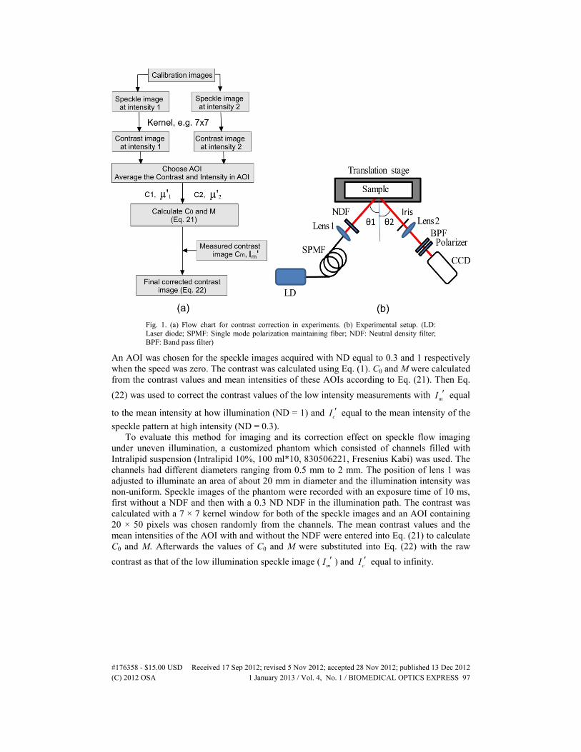
Fig. 1. (a) Flow chart for contrast correction in experiments. (b) Experimental setup. (LD: Laser diode; SPMF: Single mode polarization maintaining fiber; NDF: Neutral density filter; BPF: Band pass filter)

An AOI was chosen for the speckle images acquired with ND equal to 0.3 and 1 respectively when the speed was zero. The contrast was calculated using Eq. (1). C0 and M were calculated from the contrast values and mean intensities of these AOIs according to Eq. (21). Then Eq. (22) was used to correct the contrast values of the low intensity measurements with mI ′ equal

to the mean intensity at how illumination (ND = 1) and cI ′ equal to the mean intensity of the speckle pattern at high intensity (ND = 0.3).

To evaluate this method for imaging and its correction effect on speckle flow imaging under uneven illumination, a customized phantom which consisted of channels filled with Intralipid suspension (Intralipid 10%, 100 ml*10, 830506221, Fresenius Kabi) was used. The channels had different diameters ranging from 0.5 mm to 2 mm. The position of lens 1 was adjusted to illuminate an area of about 20 mm in diameter and the illumination intensity was non-uniform. Speckle images of the phantom were recorded with an exposure time of 10 ms, first without a NDF and then with a 0.3 ND NDF in the illumination path. The contrast was calculated with a 7 × 7 kernel window for both of the speckle images and an AOI containing 20 × 50 pixels was chosen randomly from the channels. The mean contrast values and the mean intensities of the AOI with and without the NDF were entered into Eq. (21) to calculate C0 and M. Afterwards the values of C0 and M were substituted into Eq. (22) with the raw contrast as that of the low illumination speckle image ( mI ′ ) and cI ′ equal to infinity.


5. Results

5.1. Simulation

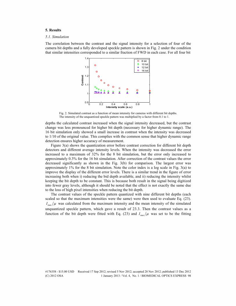
The correlation between the contrast and the signal intensity for a selection of four of the camera bit depths and a fully developed speckle pattern is shown in Fig. 2 under the condition that similar intensities corresponded to a similar fraction of FWD in each case. For all four bit

Fig. 2. Simulated contrast as a function of mean intensity for cameras with different bit depths. The intensity of the unquantized speckle pattern was multiplied by a factor from 0.1 to 1.

depths the calculated contrast increased when the signal intensity decreased, but the contrast change was less pronounced for higher bit depth (necessary for higher dynamic range). The 16 bit simulation only showed a small increase in contrast when the intensity was decreased to 1/10 of the original value. This complies with the common sense that higher dynamic range detection ensures higher accuracy of measurement.

Figure 3(a) shows the quantization error before contrast correction for different bit depth detectors and different average intensity levels. When the intensity was decreased the error increased to a maximum of 32% for the 8 bit simulation, but the error only increased to approximately 0.3% for the 16 bit simulation. After correction of the contrast values the error decreased significantly as shown in the Fig. 3(b) for comparison. The largest error was approximately 1% for the 8 bit simulation. Note the color index is a log scale in Fig. 3(a) to improve the display of the different error levels. There is a similar trend in the figure of error increasing both when i) reducing the bid depth available, and ii) reducing the intensity whilst keeping the bit depth to be constant. This is because both result in the signal being digitized into fewer gray levels, although it should be noted that the effect is not exactly the same due to the loss of high pixel intensities when reducing the bit depth.

The contrast values of the speckle pattern quantized with nine different bit depths (each scaled so that the maximum intensities were the same) were then used to evaluate Eq. (23).

maxI µ was calculated from the maximum intensity and the mean intensity of the simulated unquantized speckle pattern, which gave a result of 23.3. Then the contrast values as a function of the bit depth were fitted with Eq. (23) and maxI µ was set to be the fitting

0 0.2 0.4 0.6 0.8 10.9

1

1.1

1.2

1.3

1.4

Intensity scale (a.u.)

Con

trast

8 bit10 bit12 bit16 bit


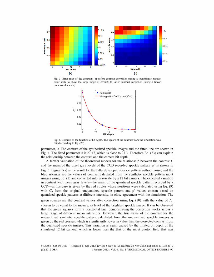
Fig. 3. Error map of the contrast: (a) before contrast correction (using a logarithmic pseudo color scale to show the large range of errors); (b) after contrast correction (using a linear pseudo color scale).

Fig. 4. Contrast as the function of bit depth. The square of the contrast from the simulation was fitted according to Eq. (23).

parameter, a. The contrast of the synthesized speckle images and the fitted line are shown in Fig. 4. The fitted parameter a is 27.47, which is close to 23.3. Therefore Eq. (23) can explain the relationship between the contrast and the camera bit depth.

A further validation of the theoretical models for the relationship between the contrast C and the mean of the pixel gray levels of the CCD recorded speckle pattern µ′ is shown in Fig. 5. Figure 5(a) is the result for the fully developed speckle pattern without noise, and the blue asterisks are the values of contrast calculated from the synthetic speckle pattern input images using Eq. (1) and converted into grayscale by a 12 bit camera. The expected variation in contrast with mean gray levels—the mean of the quantized speckle pattern recorded by a CCD—in this case is given by the red circles whose positions were calculated using Eq. (9) with C0 from the original unquantized speckle pattern and µ′ values chosen based on quantized speckle patterns at different intensity, in close agreement with the simulation. The green squares are the contrast values after correction using Eq. (10) with the value of cI ′ chosen to be equal to the mean gray level of the brightest speckle image. It can be observed that the green squares form a horizontal line, demonstrating the correction works across a large range of different mean intensities. However, the true value of the contrast for the unquantized synthetic speckle pattern calculated from the unquantized speckle images is given by the red crosses, which is significantly lower in value than the corrected contrast from the quantized speckle images. This variation is again caused by the limited bit depth of the simulated 12 bit camera, which is lower than the that of the input photon field that was

8 10 12 14 16

1.02

1.04

1.06

1.08

1.1

Bit depth

C2

SimulationFitting with C2=C02(1+a/(2N-1)


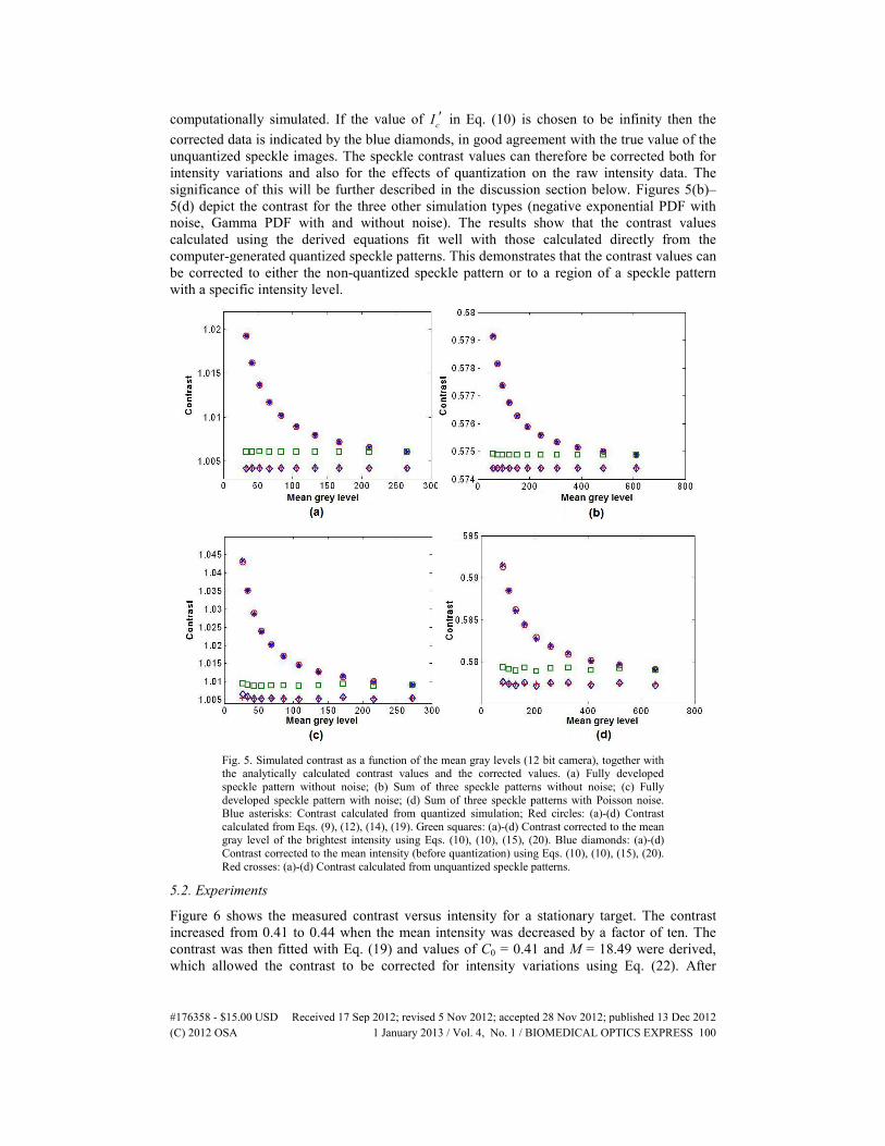
computationally simulated. If the value of cI ′ in Eq. (10) is chosen to be infinity then the corrected data is indicated by the blue diamonds, in good agreement with the true value of the unquantized speckle images. The speckle contrast values can therefore be corrected both for intensity variations and also for the effects of quantization on the raw intensity data. The significance of this will be further described in the discussion section below. Figures 5(b)–5(d) depict the contrast for the three other simulation types (negative exponential PDF with noise, Gamma PDF with and without noise). The results show that the contrast values calculated using the derived equations fit well with those calculated directly from the computer-generated quantized speckle patterns. This demonstrates that the contrast values can be corrected to either the non-quantized speckle pattern or to a region of a speckle pattern with a specific intensity level.

Fig. 5. Simulated contrast as a function of the mean gray levels (12 bit camera), together with the analytically calculated contrast values and the corrected values. (a) Fully developed speckle pattern without noise; (b) Sum of three speckle patterns without noise; (c) Fully developed speckle pattern with noise; (d) Sum of three speckle patterns with Poisson noise. Blue asterisks: Contrast calculated from quantized simulation; Red circles: (a)-(d) Contrast calculated from Eqs. (9), (12), (14), (19). Green squares: (a)-(d) Contrast corrected to the mean gray level of the brightest intensity using Eqs. (10), (10), (15), (20). Blue diamonds: (a)-(d) Contrast corrected to the mean intensity (before quantization) using Eqs. (10), (10), (15), (20). Red crosses: (a)-(d) Contrast calculated from unquantized speckle patterns.

5.2. Experiments

Figure 6 shows the measured contrast versus intensity for a stationary target. The contrast increased from 0.41 to 0.44 when the mean intensity was decreased by a factor of ten. The contrast was then fitted with Eq. (19) and values of C0 = 0.41 and M = 18.49 were derived, which allowed the contrast to be corrected for intensity variations using Eq. (22). After


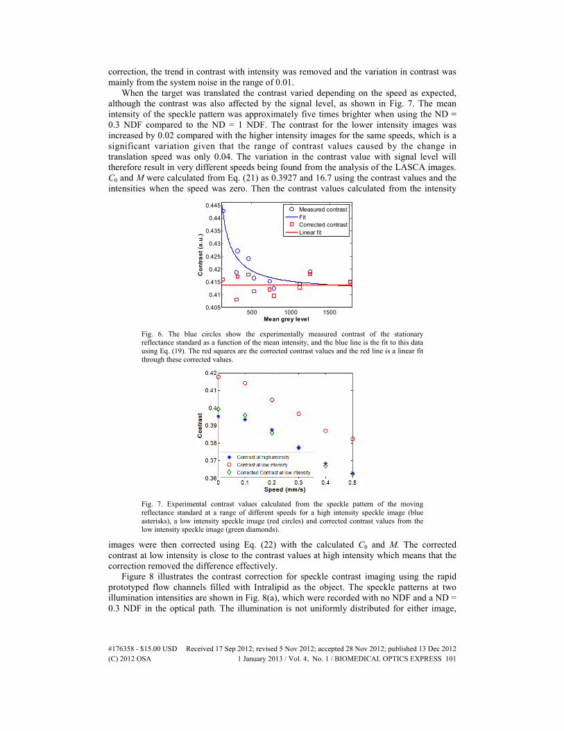
correction, the trend in contrast with intensity was removed and the variation in contrast was mainly from the system noise in the range of 0.01.

When the target was translated the contrast varied depending on the speed as expected, although the contrast was also affected by the signal level, as shown in Fig. 7. The mean intensity of the speckle pattern was approximately five times brighter when using the ND = 0.3 NDF compared to the ND = 1 NDF. The contrast for the lower intensity images was increased by 0.02 compared with the higher intensity images for the same speeds, which is a significant variation given that the range of contrast values caused by the change in translation speed was only 0.04. The variation in the contrast value with signal level will therefore result in very different speeds being found from the analysis of the LASCA images. C0 and M were calculated from Eq. (21) as 0.3927 and 16.7 using the contrast values and the intensities when the speed was zero. Then the contrast values calculated from the intensity

Fig. 6. The blue circles show the experimentally measured contrast of the stationary reflectance standard as a function of the mean intensity, and the blue line is the fit to this data using Eq. (19). The red squares are the corrected contrast values and the red line is a linear fit through these corrected values.

Fig. 7. Experimental contrast values calculated from the speckle pattern of the moving reflectance standard at a range of different speeds for a high intensity speckle image (blue asterisks), a low intensity speckle image (red circles) and corrected contrast values from the low intensity speckle image (green diamonds).

images were then corrected using Eq. (22) with the calculated C0 and M. The corrected contrast at low intensity is close to the contrast values at high intensity which means that the correction removed the difference effectively.

Figure 8 illustrates the contrast correction for speckle contrast imaging using the rapid prototyped flow channels filled with Intralipid as the object. The speckle patterns at two illumination intensities are shown in Fig. 8(a), which were recorded with no NDF and a ND = 0.3 NDF in the optical path. The illumination is not uniformly distributed for either image,

500 1000 15000.405

0.41

0.415

0.42

0.425

0.43

0.435

0.44

0.445

Mean grey level

Con

trast

(a.u

.)

Measured contrastFitCorrected contrastLinear fit


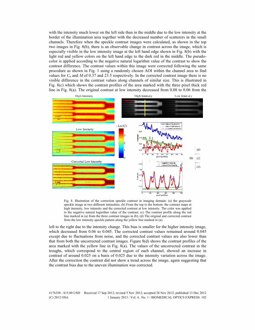
with the intensity much lower on the left side than in the middle due to the low intensity at the border of the illumination area together with the decreased number of scatterers in the small channels. Therefore when the speckle contrast images were calculated, as shown in the top two images in Fig. 8(b), there is an observable change in contrast across the image, which is especially visible in the low intensity image at the left hand edge shown in Fig. 8(b) with the light red and yellow colors on the left hand edge to the dark red in the middle. The pseudo-color is applied according to the negative natural logarithm value of the contrast to show the contrast difference. The contrast values within this image were corrected following the same procedure as shown in Fig. 1 using a randomly chosen AOI within the channel area to find values for C0 and M of 0.37 and 23.5 respectively. In the corrected contrast image there is no visible difference in the contrast values along channels of similar size. This is illustrated in Fig. 8(c) which shows the contrast profiles of the area marked with the three pixel thick red line in Fig. 8(a). The original contrast at low intensity decreased from 0.08 to 0.06 from the

Fig. 8. Illustration of the correction speckle contrast in imaging domain: (a) the grayscale speckle image at two different intensities; (b) From the top to the bottom: the contrast maps at high intensity, low intensity and the corrected contrast at low intensity. The color was applied to the negative natural logarithm value of the contrast. (c) The contrast profile along the red line marked in (a) from the three contrast images in (b); (d) The original and corrected contrast from the low intensity speckle pattern along the yellow line marked in (a).

left to the right due to the intensity change. This bias is smaller for the higher intensity image, which decreased from 0.06 to 0.045. The corrected contrast values remained around 0.045 except due to fluctuations from noise, and the corrected contrast values are also lower than that from both the uncorrected contrast images. Figure 8(d) shows the contrast profiles of the area marked with the yellow line in Fig. 8(a). The values of the uncorrected contrast in the troughs, which correspond to the central region of each channel, showed an increase in contrast of around 0.025 on a basis of 0.025 due to the intensity variation across the image. After the correction the contrast did not show a trend across the image, again suggesting that the contrast bias due to the uneven illumination was corrected.


6. Discussion

The influence of the mean intensity of the speckle pattern on the contrast comes from the quantization of the intensity, which is digitized with limited bit depth. The lower the number of bits filled, the less accurately the intensity is sampled, affecting the contrast of the quantized speckle pattern. Therefore choosing a high bit depth camera, such as 16 bit, can effectively remove the contrast bias from the change of the mean intensity, provided the signal level is high enough to make use of the additional gray levels. When the bit depth of the camera is low, it is important to take the influence of the mean gray level into consideration when calculating the contrast. It should also be noted that the effect of reducing the signal for one particular bit depth camera is similar to reducing the bit depth of the camera. However, the high intensity pixels are still better sampled in the case of reducing the average signal intensity, whereas this information would be lost if reducing the bit depth.

The significance of correcting the contrast bias from the variation of the intensity in biophotonics applications is to get a better estimate of the change in the estimated speed from the contrast, since LASCA is mainly used to measure the blood flow speed. The importance of this is illustrated by Fig. 7, where the estimated speed from the same contrast at two different intensity levels can be significantly different. In the clinical application, the intensity variation is inevitable due to the uneven illumination, and the different absorption and scattering properties of different types of tissue. Therefore the flow speed should be calculated or compared using the corrected contrast values.

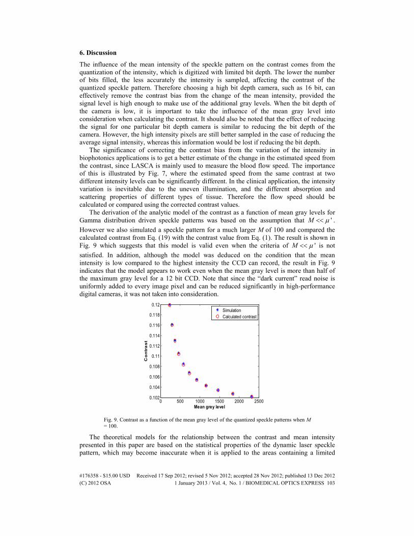
The derivation of the analytic model of the contrast as a function of mean gray levels for Gamma distribution driven speckle patterns was based on the assumption that 'M µ<< . However we also simulated a speckle pattern for a much larger M of 100 and compared the calculated contrast from Eq. (19) with the contrast value from Eq. (1). The result is shown in Fig. 9 which suggests that this model is valid even when the criteria of 'M µ<< is not satisfied. In addition, although the model was deduced on the condition that the mean intensity is low compared to the highest intensity the CCD can record, the result in Fig. 9 indicates that the model appears to work even when the mean gray level is more than half of the maximum gray level for a 12 bit CCD. Note that since the “dark current” read noise is uniformly added to every image pixel and can be reduced significantly in high-performance digital cameras, it was not taken into consideration.

Fig. 9. Contrast as a function of the mean gray level of the quantized speckle patterns when M = 100.

The theoretical models for the relationship between the contrast and mean intensity presented in this paper are based on the statistical properties of the dynamic laser speckle pattern, which may become inaccurate when it is applied to the areas containing a limited

0 500 1000 1500 2000 25000.102

0.104

0.106

0.108

0.11

0.112

0.114

0.116

0.118

0.12

Mean grey level

Co

ntr

as

t

SimulationCalculated contrast


number of speckles. Therefore in the imaging domain a large number of pixels are required to calculate the parameters for the correction.

7. Conclusions

Based on the PDF of the speckle pattern and the quantization procedure of a camera, a simplified mathematical model for the relation between contrast value and signal intensity for four types of speckle pattern has been deduced. Both the simulation and the experiments proved that this method can also be used to compensate for the contrast bias during LASCA since the contrast values found are dependent on the local mean intensity level within the sampling window. This method allows the simple correction of the contrast error induced by uneven illumination which could improve the visualization of blood flows in vascular imaging studies.

Acknowledgments

Funding for this work was provided by ERC grant 242991, and UK EPSRC and Technology Strategy Board grants EP/E06342X/1 and DT/E011101/1.


Documents

Effect of signal intensity and camera quantization on ... · Effect of signal intensity and camera quantization on laser speckle contrast analysis ... using laser speckle contrast