Embed Size (px)
Citation preview
APPROVED: Samuel Atkinson, Major Professor Kenneth Dickson, Committee Member Irene Klaver, Committee Member Ken Steigman, Committee Member W. Richard Teague, Committee Member Urs Kreuter, Committee Member Art Goven, Chair of the Department of
Biological Sciences James D. Meernik, Acting Dean of the
Toulouse Graduate School
EFFECT OF RANCHERS' MANAGEMENT PHILOSOPHY, GRAZING PRACTICES,
AND PERSONAL CHARACTERISTICS ON SUSTAINABILITY INDICES
FOR NORTH CENTRAL TEXAS RANGELAND
Wayne Becker, B.S., M.S.
Dissertation Prepared for the Degree of
DOCTOR OF PHILOSOPHY
UNIVERSITY OF NORTH TEXAS
December 2011
Becker, Wayne. Effect of ranchers’ management philosophy, grazing practices, and
personal characteristics on sustainability indices for north central Texas rangeland. Doctor of
Philosophy (Environmental Science), December 2011, 216 pp., 45 tables, 24 figures, references,
92 titles.
To assess sustainability of privately owned rangeland, a questionnaire was used to
gathered data from ranches in Cooke, Montague, Clay, Wise, Parker, and Jack counties in North
Central Texas. Information evaluated included: management philosophy, economics, grazing
practices, environmental condition, quality of life, and demographics. Sustainability indices
were created based on economic and land health indicator variables meeting a minimum
Cronbach‘s alpha coefficient (α = 0.7). Hierarchical regression analysis was used to create
models explaining variance in respondents’ indices scores. Five predictors explained 36% of the
variance in rangeland economic sustainability index when respondents: 1) recognized
management inaction has opportunity costs affecting economic viability; 2) considered forbs a
valuable source of forage for wildlife or livestock; 3) believed governmental assistance with
brush control was beneficial; 4) were not absentee landowners and did not live in an urban area
in Texas, and; 5) valued profit, productivity, tax issues, family issues, neighbor issues or weather
issues above that of land health. Additionally, a model identified 5 predictors which explained
30% of the variance for respondents with index scores aligning with greater land health
sustainability. Predictors indicated: 1) fencing cost was not an obstacle for increasing livestock
distribution; 2) land rest was a component of grazing plans; 3) the Natural Resource
Conservation Service was used for management information; 4) fewer acres were covered by
dense brush or woodlands, and; 5) management decisions were not influenced by friends.
Finally, attempts to create an index and regression analysis explaining social sustainability was
abandoned, due to the likely-hood of type one errors.
These findings provide a new line of evidence in assessing rangeland sustainability,
supporting scientific literature concerning rangeland sustainability based on ranch level
indicators. Compared to measuring parameters on small plots, the use of indices allows for
studying replicated whole- ranch units using rancher insight. Use of sustainability indices may
prove useful in future rangeland research activities.

ii
Copyright 2011
by
Wayne Becker
iii
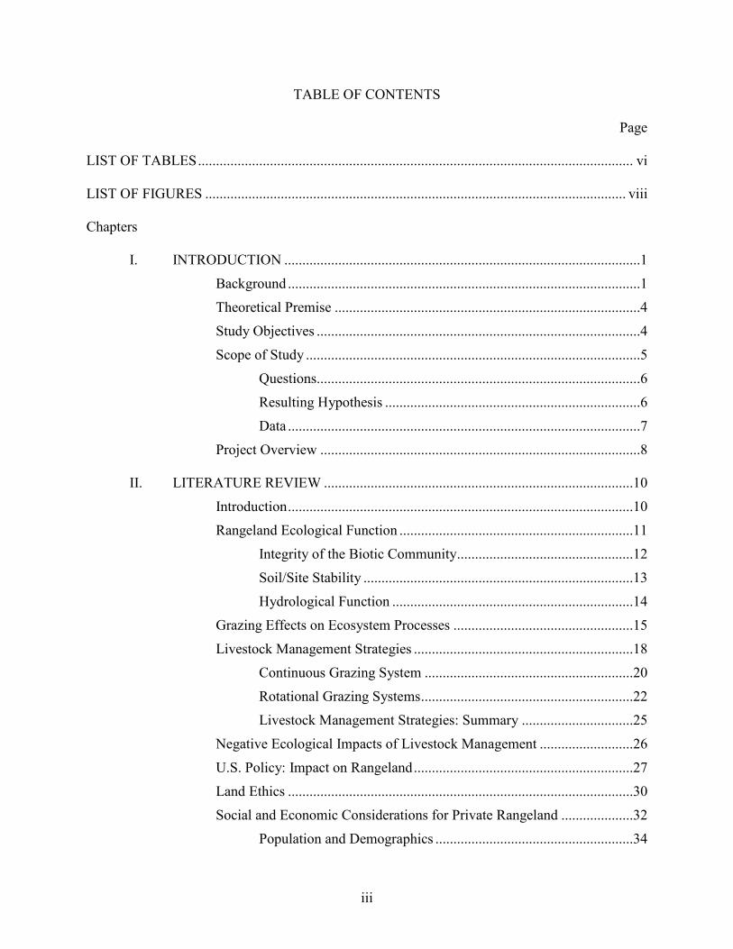
TABLE OF CONTENTS
Page LIST OF TABLES ......................................................................................................................... vi LIST OF FIGURES ..................................................................................................................... viii Chapters
I. INTRODUCTION ...................................................................................................1
Background ..................................................................................................1
Theoretical Premise .....................................................................................4
Study Objectives ..........................................................................................4
Scope of Study .............................................................................................5
Questions..........................................................................................6
Resulting Hypothesis .......................................................................6
Data ..................................................................................................7
Project Overview .........................................................................................8 II. LITERATURE REVIEW ......................................................................................10
Introduction ................................................................................................10
Rangeland Ecological Function .................................................................11
Integrity of the Biotic Community .................................................12
Soil/Site Stability ...........................................................................13
Hydrological Function ...................................................................14
Grazing Effects on Ecosystem Processes ..................................................15
Livestock Management Strategies .............................................................18
Continuous Grazing System ..........................................................20
Rotational Grazing Systems ...........................................................22
Livestock Management Strategies: Summary ...............................25
Negative Ecological Impacts of Livestock Management ..........................26
U.S. Policy: Impact on Rangeland .............................................................27
Land Ethics ................................................................................................30
Social and Economic Considerations for Private Rangeland ....................32
Population and Demographics .......................................................34
iv
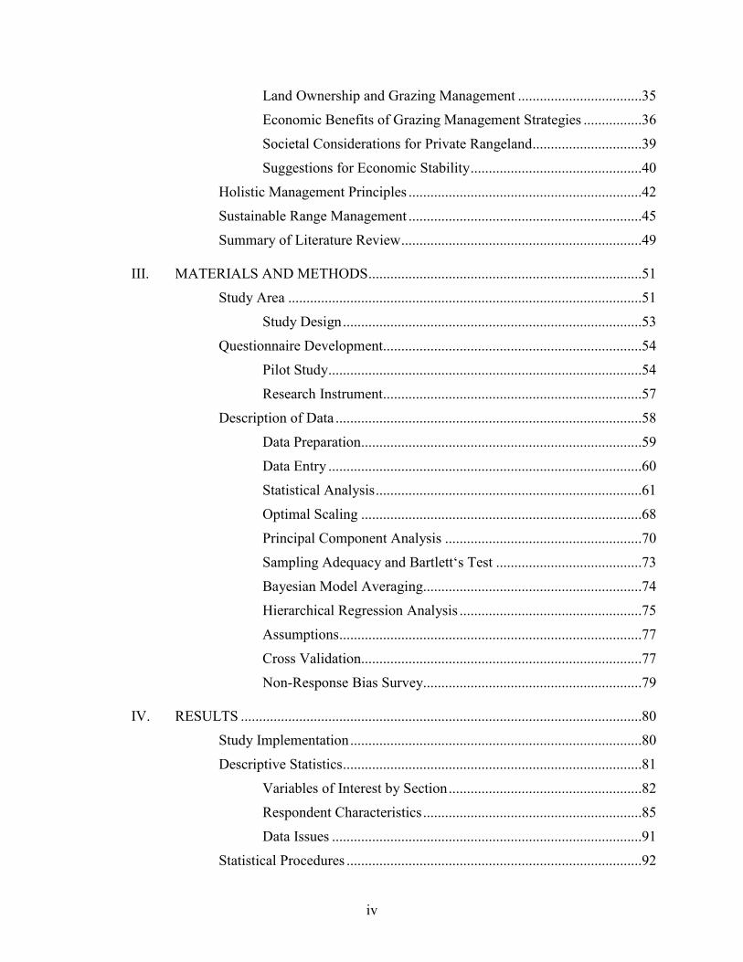
Land Ownership and Grazing Management ..................................35
Economic Benefits of Grazing Management Strategies ................36
Societal Considerations for Private Rangeland ..............................39
Suggestions for Economic Stability ...............................................40
Holistic Management Principles ................................................................42
Sustainable Range Management ................................................................45
Summary of Literature Review ..................................................................49 III. MATERIALS AND METHODS ...........................................................................51
Study Area .................................................................................................51
Study Design ..................................................................................53
Questionnaire Development.......................................................................54
Pilot Study ......................................................................................54
Research Instrument.......................................................................57
Description of Data ....................................................................................58
Data Preparation.............................................................................59
Data Entry ......................................................................................60
Statistical Analysis .........................................................................61
Optimal Scaling .............................................................................68
Principal Component Analysis ......................................................70
Sampling Adequacy and Bartlett‘s Test ........................................73
Bayesian Model Averaging............................................................74
Hierarchical Regression Analysis ..................................................75
Assumptions ...................................................................................77
Cross Validation.............................................................................77
Non-Response Bias Survey............................................................79 IV. RESULTS ..............................................................................................................80
Study Implementation ................................................................................80
Descriptive Statistics ..................................................................................81
Variables of Interest by Section .....................................................82
Respondent Characteristics ............................................................85
Data Issues .....................................................................................91
Statistical Procedures .................................................................................92
v
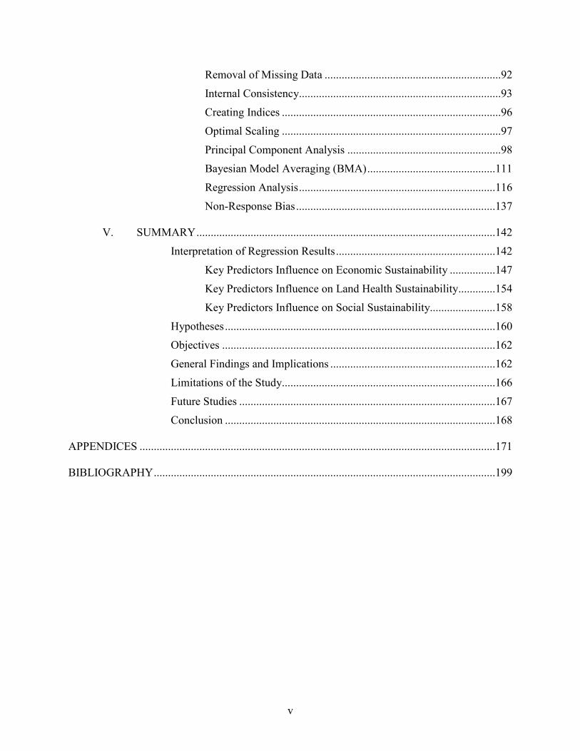
Removal of Missing Data ..............................................................92
Internal Consistency.......................................................................93
Creating Indices .............................................................................96
Optimal Scaling .............................................................................97
Principal Component Analysis ......................................................98
Bayesian Model Averaging (BMA) .............................................111
Regression Analysis .....................................................................116
Non-Response Bias ......................................................................137 V. SUMMARY .........................................................................................................142
Interpretation of Regression Results ........................................................142
Key Predictors Influence on Economic Sustainability ................147
Key Predictors Influence on Land Health Sustainability .............154
Key Predictors Influence on Social Sustainability.......................158
Hypotheses ...............................................................................................160
Objectives ................................................................................................162
General Findings and Implications ..........................................................162
Limitations of the Study...........................................................................166
Future Studies ..........................................................................................167
Conclusion ...............................................................................................168 APPENDICES .............................................................................................................................171 BIBLIOGRAPHY ........................................................................................................................199
vi
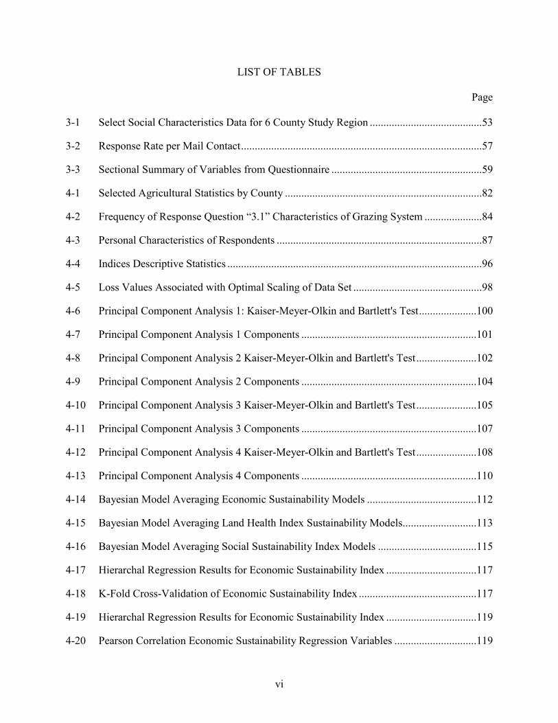
LIST OF TABLES
Page 3-1 Select Social Characteristics Data for 6 County Study Region .........................................53
3-2 Response Rate per Mail Contact ........................................................................................57
3-3 Sectional Summary of Variables from Questionnaire .......................................................59
4-1 Selected Agricultural Statistics by County ........................................................................82
4-2 Frequency of Response Question “3.1” Characteristics of Grazing System .....................84
4-3 Personal Characteristics of Respondents ...........................................................................87
4-4 Indices Descriptive Statistics .............................................................................................96
4-5 Loss Values Associated with Optimal Scaling of Data Set ...............................................98
4-6 Principal Component Analysis 1: Kaiser-Meyer-Olkin and Bartlett's Test .....................100
4-7 Principal Component Analysis 1 Components ................................................................101
4-8 Principal Component Analysis 2 Kaiser-Meyer-Olkin and Bartlett's Test ......................102
4-9 Principal Component Analysis 2 Components ................................................................104
4-10 Principal Component Analysis 3 Kaiser-Meyer-Olkin and Bartlett's Test ......................105
4-11 Principal Component Analysis 3 Components ................................................................107
4-12 Principal Component Analysis 4 Kaiser-Meyer-Olkin and Bartlett's Test ......................108
4-13 Principal Component Analysis 4 Components ................................................................110
4-14 Bayesian Model Averaging Economic Sustainability Models ........................................112
4-15 Bayesian Model Averaging Land Health Index Sustainability Models ...........................113
4-16 Bayesian Model Averaging Social Sustainability Index Models ....................................115
4-17 Hierarchal Regression Results for Economic Sustainability Index .................................117
4-18 K-Fold Cross-Validation of Economic Sustainability Index ...........................................117
4-19 Hierarchal Regression Results for Economic Sustainability Index .................................119
4-20 Pearson Correlation Economic Sustainability Regression Variables ..............................119
vii
4-21 Collinearity Statistics Economic Sustainability Regression Variables ............................120
4-22 K-Fold Cross-Validation of Economic Sustainability Index ...........................................121
4-23 Hierarchal Regression Results for Land Health Sustainability Index .............................122
4-24 DFFit Statistic for Land Health Mahalaboni’s Distance Scores ......................................123
4-25 Hierarchal Regression Results for Land Health Sustainability Index .............................125
4-26 Correlations Land Health Index .......................................................................................125
4-27 Collinearity Statistics Land Health Sustainability Index .................................................126
4-28 K-Fold Cross-Validation of Land Health Sustainability Index .......................................127
4-29 Hierarchal Regression Results for Social Sustainability Index .......................................128
4-30 DFFit Statistic for Land Health Mahalaboni’s Distance Scores ......................................130
4-31 DFFit Statistic for Land Health Mahalaboni’s Distance Scores-2 ...................................131
4-32 Hierarchal Regression Results for Social Sustainability Index .......................................134
4-33 Hierarchal Regression Results for Social Sustainability Index-2 ....................................135
4-34 Pearson Correlation Social Sustainability Index..............................................................136
4-35 Collinearity Statistics Social Sustainability Index ...........................................................136
4-36 K-Fold Cross-Validation of Social Sustainability Index .................................................137
4-37 Non-Response Descriptive Statistics for Select Variables ..............................................140
4-38 Percentages Non-Respondents vs. Respondents ..............................................................140
4-39 Non-Response Hypothesis Test Summary.......................................................................141
5-1 Predictors Relationship with the Economic Sustainability Index ....................................144
5-2 Predictors Relationship with the Land Health Sustainability Index ................................145
5-3 Predictors Relationship with the Land Health Sustainability Index ................................146
viii
LIST OF FIGURES
Page
3-1 Location of study area, in relation to Texas and the West Cross Timbers ........................52
4-1 Land location by county.....................................................................................................88
4-2 Way respondent is associated with the land ......................................................................88
4-3 Respondent level of education ...........................................................................................89
4-4 Respondent source of continuing education ......................................................................89
4-5 Years living on ranch .........................................................................................................90
4-6 If not living on ranch, location of home ............................................................................90
4-7 Respondent income by category ........................................................................................91
4-8 Scree plot Principal Component Analysis 1 ......................................................................99
4-9 Scree plot Principal Component Analysis 2 ....................................................................102
4-10 Scree plot Principal Component Analysis 3 ....................................................................105
4-11 Scree plot Principal Component Analysis 4 ....................................................................108
4-12 Economic index standardized residual values .................................................................120
4-13 Economic index normal probability plot .........................................................................120
4-14 Economic index Mahalaboni’s distance plot ...................................................................121
4-15 Box plot of Mahalaboni’s distance scores for land health index .....................................123
4-16 Standardized residuals histogram for land health sustainability index ............................126
4-17 Normal probability plot for land health sustainability index residuals ............................126
4-18 Box plot for Mahalanobi’s distance scores of land health sustainability index ...............127
4-19 Box plot for Mahalaboni’s distance scores of social sustainability index .......................129
4-20 Box plot for Mahalanobi’s distance scores of social sustainability index .......................131
4-21 Mahalaboni’s distance score (Q-Q) plot for social sustainability index ..........................133
4-22 Standardized residual histogram for social sustainability index ......................................137

ix
4-23 Box plot for Mahalanobi’s distance scores of social sustainability index .......................137
1
CHAPTER I
INTRODUCTION
Background
The present state of health of U.S. rangelands is a matter of sharp debate, even for
government agencies working with rangeland assessments. Valuable products are associated
with these grasslands, including forage for domestic and wild animals, species habitat, water
storage and filtration, carbon sequestration, recreation, open space, and a way of life for
rangeland-dependent rural communities. These products are aligned with economic, ecological.
and social parameters (Maczko et al., 2004).
Lands designated as ―grazing land‖ encompass 25.9% of all land in the U.S. (Lubowiski
et al., 2006). These grazing lands are a result of the anthropocentric shift of free-range wild
herbivores to a system which is sometimes characterized by overgrazing and loss of ecological
function caused by domesticated livestock. The relationship between the ecosystem and
livestock grazing is often the primary reason for the concern about rangeland health (Belsky et
al., 1999; Centeri et al., 2009). The concern over animal impact on the environment is one of the
major reasons for the debate concerning rangeland. The opposite belief is that grazing by
ungulates was instrumental in the evolutionary history of grassland ecosystems (Michunas et al.,
1988; Knapp et al., 1999) and grazing of indigenous rangeland is one of the most sustainable
forms of agriculture known (Frank and McNaughton , 2002; Heitschmidt et al., 2004).
The interaction of livestock with the environment is very complex. Different scientists
looking at the same data have come to different conclusions. Additional problems are incurred
when reconciling grazing land management results from experimental studies, with commonly
2
held beliefs and perceptions. This is especially true regarding outcomes derived from
implementation of various grazing strategies (Briske et al., 2008).
A primary issue with reconciliation of experimental evidence and perceived rangeland
management outcomes has been the scale of field experiments. Generally, scientific studies have
not conformed to the scale of grazing operations because of the importance of replicating
treatments in experimental research and the limited availability of land and other resources for
conducting such research. It is impossible to capture, in small-scale research trials, the
complexity of rangeland resources in operational scale grazing systems (Teague et al., 2008;
Laca, 2009).
Furthermore, managers must adapt to changing biophysical and socio-economic
conditions. These include variables that are extremely difficult or impossible to address in short-
term and small scale grazing experiments, such as, changing weather conditions and variations in
grazing behavior of animals. As a result, the high number of variables affecting ranch-scale
management makes it virtually impossible to use traditional experimental protocols to compare
alternative management schemes at real-world operational scales. Even though pastoralist
knowledge is more focused on productivity than on maintaining ecosystem processes (Bollig and
Schulte, 1999), Knapp and Fernandez-Gimenez (2009) concluded that ranchers in the West have
gained insight about natural systems through daily interaction and management of landscapes.
Through interviews, they found that ranch managers‘ knowledge complemented scientific
knowledge, especially concerning active knowledge applied to management decisions,
embedded knowledge from living in place, and integrative knowledge that links ecological,
economic, and social aspects of rangeland systems.
As Maczko et al. (2004) indicated economic, ecologic, and social elements may be
visualized as one leg of a 3-legged stool, with each aspect of sustainability representing a leg.
3
Understanding the complex interactions that occur between grazing management and each of
these three elements will ultimately lead to conclusions concerning the sustainability of
rangelands.
Perception is the process of attaining an understanding of information and is a result of
interplays between past experiences and personal interpretation (Pomerantz, 2003). While
experimental studies are vital, management‘s perception of benefits associated with grazing
systems are even more crucial for successful implementation of sustainable ranch management
practices; only ranch-level, adaptable grazing system management is capable of addressing all of
the variables associated with sustainability of mid to tall-grass prairie ecosystems.
Overgrazing, drought, erosion, and other human and naturally induced stressors have
caused severe degradation in the past. In many areas, rangeland remnants are all that remain of
vast sections of mid to tall-grass prairies. These remnants are very much at risk of damage due to
the mismanagement of livestock and increasing human population. Costa and Reham (2005)
have shown that the traditional decisions to retain livestock, even at the expense of the
environment, may be as philosophic as they are economic. Deliberate, high-stocking rate
decisions appear paradoxical, even irrational given the state of knowledge regarding the
consequences of overgrazing. The phenomenon appears to be linked with objectives of livestock
managers. Indications are that producers view cattle ownership as a means to ensure they are
able to continue land ownership, as a source of security and liquidity, and as a way of life worthy
of passing to the next generation.
Sustainable resource management has evolved as the logical extension of the application
of sustainable development principles to land management (Shields and Bartlett, 2002).
Implementation of sustainable grazing practices is of value to protect vital natural resources such
as rivers, streams and aquifers as well as to increase productivity of agricultural practices without
4
increasing use of non-renewable resources. The application of appropriate grazing management
systems has been widely found to be critical for the continued ecological health and agricultural
sustainability of rangelands around the world (Klipple & Costello, 1960; Holechek, 1994; Ward,
1999).
Theoretical Premise
The theoretic premise put forward by this study is a direct response to the issues
described in the background. The specific premise is that a method which investigates each
aspect of rangeland sustainability separately (economic, land health, and social) is necessary.
Doing so will be useful when land owners and agency personnel are assessing different
perspectives known to be factors affecting the ability of mankind to utilize this natural resource
sustainably; benefitting from its goods and services today, while preserving these goods and
services so that future generations can benefit also. Additionally, when investigating aspects of
rangeland sustainability, a study must be conducted on the whole-ranch level; whereas, small
scale studies have proven to further divide the opinions within the scientific community.
The difficult task of assessing rangeland sustainability can be addressed by questioning
ranch managers about their economic situation, rangeland physical properties, social satisfaction,
management philosophy, grazing practices and personal characteristics. The economic
information, rangeland physical properties, and social satisfaction could be the basis for
indicators of sustainability. The questions concerning philosophy, grazing management and
personal characteristics could be used to assess impact on sustainability.
Study Objectives
Range professionals have assigned various degrees of importance to different processes
in nature (Naeem, 2002). ―Applied management sciences bridge the gap between ecological
5
information and the achievement of desired management goals by integrating knowledge from
diverse disciplines. They evaluate management consequences within a research-based theoretical
framework of ecological processes and how they affect ecological, economic, and social factors
important to management‖ (Teague et al,. 2008). This analogy links closely with Sydorovych
and Wossink (2008) and Calker (2005), who identified sustainability for agricultural systems in
terms of economics, internal social, external social and ecological parameters. ―As competing
demands contend for increasingly limited rangeland resources, consistent, comparable economic,
social and ecological data is necessary for informed decision-making regarding tradeoffs among
goods and services derived from rangelands‖ (Maczko et al., 2004). The research reported here
contributes new data that should be useful in this decision-making arena.
The specific objectives of the study were to contribute to the knowledge and
understanding of some of the key grazing management elements essential to sustainable
rangeland management as described by the 2003 SRR Executive Summary (West and Herrick,
2003), specifically:
1. Contribute to the knowledge base for research by agencies, universities, and
organizations focused on developing methods to address data gaps and research
needs associated with criteria and indicators,
2. Aid in improved accountability for rangelands stakeholders through multi-scale,
coordinated data reporting.
3. Provide a basis for stakeholder dialogue at local, regional, and national scales and
expanded understanding of rangeland sustainability.
4. Gain an understanding of range management philosophy, practices, and personal
characteristics that are indicators of sustainable management at the whole-ranch
scale.
Scope of Study
This study sought to understand the relationship between grazing management decisions
and perception regarding long-term rangeland sustainability in whole-ranch enterprises.
6
Information was gathered, via a formal survey instrument, on a large number of variables related
to perceptions of land health, rangeland productivity, economic viability, quality of life, and
cultural experiences from the study group, which was comprised from rangeland scientists in the
north Texas area. The variables were reduced to a set of factors that aid in understanding
motivation concerning implementation of rangeland sustainability practices. The results of these
surveys should be useful for the following reasons:
1. Important indices of critical factors affecting perceptions have been developed
and could be used to develop further models that explain variations in grazing
system perceptions.
2. Results can be utilized to develop effective marketing tools to promote the
adoption of grazing management systems that enhance ecosystem sustainability.
3. The results comprehensively inform conflicting viewpoints regarding the benefits
of planned, rotational grazing practices.
Questions
Specifically the study attempted to answer the following questions:
1. What are land managers perceptions of sustainable grazing strategies based on whole-
ranch observations?
2. What management practices are ranch managers implementing?
3. What are the obstacles for land managers to implement perceived sustainable range
management practices?
4. How do management practices relate to sustainability measures? 1. Economic; 2.
Social and; 3. Ecological?
5. What is the relationship between rangeland management practices that are perceived
as sustainable and rangeland management practices that are being implemented?
6. Do managers using any particular grazing strategy, identified as contributing to the
sustainability of rangeland, have any identifying characteristics? (e.g. live on their
land, are long term residents, depend on their land for a significant amount of their
total household income, operate livestock enterprises with multiple classes of animals
(e.g. breeding cows, heifers, stokers, small stock, etc) or, operate both livestock and
wildlife enterprises more likely to use rotational grazing systems?)
Resulting Hypotheses
The questions above have led to the following hypotheses:
7
1. Land manager perceptions of sustainability, based on whole-ranch observations will
center on productivity and profit.
2. Management practices being implemented will vary widely.
3. Land managers will limit implementation of grazing strategies perceived as sustainable
based on labor and cash flow.
4. Rangeland Sustainability will be predicted by grazing management practices, philosophy,
and land owner characteristics.
5. Findings concerning landowner grazing management, via the survey instrument, will
compliment physical, experimental studies, solidifying whole-ranch assessment of
ecological sustainability.
Data
A survey of livestock managers, operating an enterprise consisting of 500 acres or more
of native rangeland, was conducted. Managers in Cooke, Montague, Clay, Jack, Wise, and
Parker Counties in north central Texas were the targeted population. Data collected included:
Demographic data; Personal philosophy on sustainability; Management practices being
implemented; Personal perception of identified components of ecosystem functionality for
respondent ranch; personal perception of economic viability for respondent ranch; Personal
perception of social issues for the respondent ranch.
These data were organized into questionnaires based on a series of strategic processes.
Initially a preliminary study was conducted, especially designed around the livestock managers‘
survey. The questionnaire was developed based on information reported in current grazing
management literature and range management text books. Conducting the preliminary study was
beneficial for several reasons. It helped to evaluate the survey instrument for comprehension by
the reader, response rate, duplication, and usefulness of answers. Also, the application of
statistical methods helped to identify interrelationships among the large number of variables.
A focus group was conducted in an effort to fully understand predominant whole-ranch
grazing management perceptions pertaining to economic, social, and ecological outcomes. As
suggested by Briske et al. (2008), this circumstantial evidence, derived from successful grazing
8
manager experiences, may be compared with experimental research to gain valuable insight and
develop a more robust approach to understanding and implementing successful grazing
management. Qualitative data collected from our focus group were documented and used to
develop the questionnaire for thorough assessment of whole-ranch management.
A formal survey was conducted to identify grazing management strategies that are
perceived by ranchers to best achieve whole-ranch business objectives and ecosystem enhancing
practices for mid to tall-grass rangelands in the USA. Data collected were used to evaluate
perceptions regarding the effect of planned grazing systems on sustainable agricultural
production in mid to tall-grass rangelands. Surveys addressed issues of sustainability questions
concerning land health; rangeland productivity and economic viability; and quality of life and
cultural experiences.
Finally, there was a test for non-response bias. This was conducted by sending a second,
but short non-response survey. Especially, of interest was demographic data, to test if non-
respondents were a representative section of the population, or if non-respondents were biased in
one direction or another.
Data were collected and evaluated for statistical methodology. SPSS and R-2.13.0
computer software were used to perform multivariate analysis. Information was reduced to
create indices from perception data. These data was compared with management practice and
with respondent characteristics. Statistical analysis served to identify key variables that are
indicators of perceived sustainable rangeland livestock management.
Project Overview
The overall goal of this research was to identify grazing management strategies that
promote the long-term productivity and ecological health of grazing land as identified from the
9
whole-ranch perspective. Technical information obtained can be used to improve awareness by
the ranch manager and the public concerning grazing management strategies that best correlate
with enhanced rangeland sustainability.
The study was submitted for approval to UNT‘s Institutional Review Board (IRB) for
approval (Human Subjects Application No.10-235). It was determined to qualify for an
exemption from further review.
The remainder of this document is divided into four main sections. The first is an in depth
look at the scientific literature available concerning rangeland grazing management strategies
and rangeland sustainability principles especially within the context of private land management
in the United States. Second there is an overview of the materials and methods involved in
developing and implementing this study. The third section is a presentation of the results and an
analysis of the data collected. Finally, the findings of the study are summarized in accordance
with the stated objectives which are listed above; future study needs are suggested.
10
CHAPTER II
LITERATURE REVIEW
Introduction
Forty to fifty percent of the terrain in the United States is rangeland. More than half is
privately owned (Buckhouse et al., 1994; Lubowski et al., 2006). A large percentage of
rangelands consist primarily of native plant communities managed, typically for livestock
production, with 587 million acres, 25.9% of the land in the U.S. being implicated as ―grazing
land‖ (Lubowiski et al., 2006).
It is easy to see that private management of such a large portion of land in the U.S. has a
very significant impact on many environmental concerns. Grazing of livestock is extremely
important to the majority of the land management issues concerning rangeland. This literature
review will attempt to explore the issues related to managing livestock on rangeland in the U.S.
To explore this topic thoroughly, one must investigate the ecological and philosophic
literature that contributes to an understanding of livestock management. The major sections of
this review are as follows:
1. Introduction
2. Rangeland Ecological Function
3. Grazing Effects on Ecosystem Function
4. Livestock Management Strategies
5. Negative Ecological Impacts of Livestock Management
6. U.S. Policy: Impact on Rangeland
7. Land Ethics
8. Social and Economic Considerations for Private Rangeland
9. Holistic Management Principles
10. Sustainable Range Management
11. Conclusion
11
Select literature that is sited helps the reader gain an understanding of range management in
the U.S. It will investigate issues and impacts associated with private land management that are
necessary to fully understand the concepts related to ongoing debate concerning preferable
grazing strategies. Finally, it will review concepts that go beyond the debate, reviewing
literature that is trying to put the pieces of land management concepts together: ecological,
social, and economic.
Rangeland Ecological Function
Rangeland ―health‖ is a term that is used by range managers to assess the environmental
integrity of the land. The Natural Resource Conservation Service (NRCS) (2000) states there are
three main attributes of rangeland that collectively define rangeland health. They are closely
related, yet separate. These are biological and physical attributes which are often used as
indicators of functional status of ecological processes and site integrity:
Integrity of the biotic community – The capacity of the site to support
characteristic functional and structural communities in the context of normal
variability; to resist loss of this function and structure due to disturbance; and to
recover following disturbance.
Soil/site stability – The capacity of the site to limit redistribution and loss of soil
resources (including nutrients and organic matter) by wind and water.
Hydrologic function - The capacity of the site to capture, store, and safely release
water from rainfall, run-on, and snow melt, to resist a reduction in this capacity,
and to recover this capacity following degradation.
The attributes are susceptible to changes caused by disturbance in climate and
precipitation patterns, or disturbance caused associated with land use.
12
Integrity of the Biotic Community
The central assertion of a relationship between biodiversity and ecosystem function is
that greater diversity is associated with higher ecosystem stability. Heterogeneity is the
precursor to biological diversity at most levels of ecological organization and should serve as the
foundation for conservation and ecosystem management (Christensen, 2003). Rangelands have
been described as inherently heterogeneous because composition, productivity, and diversity are
highly variable across multiple scales (Ludwig and Tongway, 1995; Fuhlendorf and Smeins,
1998). Mac Arthur (1972) suggested that with increases of alternative pathways for energy flow
within an ecosystem, the less likely that pathway destruction or disruption would unsettle the
system. Supporting these claims McCann (2000), notes that decreasing biodiversity will be
accompanied by less but stronger interactions within ecosystems and a decrease in ecosystem
stability (Deregibus et al., 2001).
A heterogeneous patchwork on rangelands can result from differential timing of
disturbances and corresponding out-of-phase succession among patches, spatial variability of
resources associated with topographic and edaphic patterns, or competitive interactions among
plant species (Fuhlendorf and Smeins, 1998; Fuhlendorf and Engle, 2001). Further, plant species
diversity and richness are affected by grazing management. Grazing enhances diversity at low
rates but reduces it at high rates (Mariott et al., 2009). The duration of agricultural intensification
appears to set the rate of recovery, with high variability between situations (Bakker and
Berendse, 1999).
It is also important to consider observations of the impacts of grazing on species diversity
associated with non-plant species. Sward structure usually changes rapidly after a reduction in
management intensity. Reduction of agriculture-use intensity generally results in more dead
material and more height heterogeneity (Vickery et al., 2001). Reduction in sward height caused
13
by intensive grazing negatively affects some insects and arachnids, especially the smaller and
more sedentary species, however, abundance of arthropods increased more substantially in
relation to tussocks than swards (Dennis et al., 1998). Vegetation structure is also important to
birds. It has been shown that shorter swards favor birds foraging on soil invertebrates, but taller
swards favor those feeding on seeds or foliage (Atkinson et al., 2005; Buckingham et al., 2006).
Soil/Site Stability
Grass steppe represented the most desirable state in term of livestock production and soil
stability, while shrub steppe represented the most degraded and least productive state (Beeskow
et al., 1995). According to Wilson and Tupper (1982), range condition should be based
primarily on soil stability as soil degradation is the most serious manifestation of a decline in
range condition. Wind erosion of soils is likely to play an important role in the desert grasslands
of the southwestern United States, which have experienced dramatic vegetation changes
including extensive encroachment by shrublands over the past 150 years (Buffington and Herbel,
1965; Allred, 1996; Gibbens et al., 2005). Li et al. (2007) suggests that shrubs are relatively
ineffective at reducing wind erosion and nutrient loss compared to grasses. Vegetation changes
and soil degradation processes are closely related and may be site specific. Bosch and Kellner
(1991) emphasized the importance of understanding the process of rangeland degradation before
assessing the range condition of any area.
Soil erosion and sediment delivery from agricultural areas are responsible for the supply
of sediment-associated nutrients, pesticides and heavy-metal contaminants in many rivers and
streams (Steegen et al., 2001; Verstaeten and Poesen, 2002; and Lal., 2003). Sediment transport
capacity is 10 times greater for degraded pasture than pasture in that is not degraded (Verstraeten
et al., 2007).
14
Hydrological Function
Scientific studies documenting hydrologic changes in rangelands are most often
associated with heavy grazing intensities, although these changes do not increase linearly with
grazing intensity (Naeth and Chanasyk, 1995). Increased stocking rates negatively affected
water infiltration into the soil (Abdel-Magid et al., 1987) and increased stream sedimentation
(Knight and Heightschmidt, 1987). The cause of the negative hydrological effect, as described
by Knight and Heightschmidt (1987), is changing surface factors such as aggregate stability,
surface roughness, litter cover, total grass and standing crop, combined with soil properties.
Likewise, Warren et al. (1986), found that increased stocking rates have negative effects on soil
properties (increased bulk density, disruption of biotic crust, reduced aggregate stability and
aggregate size distribution) due to physical effects on the soil and changes in the vegetation
towards dominance by lower seral plants. These effects are positively correlated with the
distribution and frequency of animal trampling. The same study indicated that managing for
grassland dominated by high seral plants improves hydrological function. Similarly, Pluhar et al.
(1987) found that infiltration increased and sediment production declined as vegetation standing
crop and cover increased.
Rest appears to be the key to soil hydrologic stability. In order to avoid long-term
progressive degradation, rest periods must be of sufficient length to allow full recovery of the
soil hydrologic condition prior to the reoccurrence of livestock impact. It seems logical that any
increase in stocking rate must, therefore, be accompanied by an increase in the length of the rest
period in order to compensate for the greater impact (Warren et al., 1986).
15
Grazing Effects on Ecosystem Processes
The relationship between the ecosystem and the anthropogenic practice of livestock
grazing is very complex. In addition to affecting the three ecological functions of rangeland,
defoliation, trampling, and mineral deposition have varied affects on rangeland health and
rangeland processes. Grazing affects multiple rangeland characteristics including biomass, soil
nutrients, soil carbon, plant species composition, and forage quality (Teague et al., 2004).
Grazing alters plant physiological processes and nutrient cycling (Booth et al., 2003).
Rangeland ecologists generally accept that grazing by ungulates was instrumental in the
evolutionary history of grassland ecosystems (Milchunas et al., 1988, Knapp et al., 1999, Frank
and McNaughton, 2002). Because of this belief and other factors, to be discussed later, several
scientists have proposed that grazing of indigenous rangeland is one of the most sustainable
forms of agriculture known (Heitschmidt et al., 2004, Frank and McNaughton, 2002). At the
same time, there are many studies that implicate grazing as a very detrimental factor affecting
rangeland (Centeri et al., 2009; Belsky et al., 1999). Another controversial hypothesis is that
herbivory may, in some situations, increase range productivity (Belsky, 1986; McNaughton,
1989; Verkaar, 1986; Crawley, 1987; Hobbs and Swift, 1988; Westoby, 1989).
Natural rangeland communities are constantly responding to the effects of the most recent
disturbance, in most cases, never achieving a steady-state or climax stage. The absence of these
disturbances in grassland ecosystems results in a decline in species diversity and deterioration of
physical structure (Picket and White, 1985). Once disturbances cause damage beyond threshold
levels, it may never be possible to restore ecosystem functionality. Thresholds represent a
transition boundary which, when crossed, results in a new, degraded, stable state that is not
easily reversed without significant inputs of resources (NRCS, 2000). Severely degraded
16
rangelands have the propensity to shift to a stable, shrub-dominated state that will not return their
original composition even with elimination of further grazing (Christensen et al., 2003).
Due to the complexity of ecological processes and their interrelationships, it is usually
difficult and/or expensive to directly measure site integrity and the status of ecological processes.
Therefore, biological and physical attributes are often used to indicate the functional status of
ecological processes and site integrity (USGS, 2002). Complicating the relationship between
grazing and the ecosystem still further is the variability between sites in relation to disturbance
response levels. This indicates that rangeland management will necessarily vary from one
location to the next.
Grazing management is the manipulation of grazing and browsing animals to accomplish
desired results, which generally include both plant and animal performance. Critical factors with
grazing management include the amount of plant material remaining after defoliation and the
timing interval between defoliations. The most basic analysis of grazing management
acknowledges management decisions are contingent on stocking rates and rotation timing
(Hanselka et al., 2009). Additionally, grazing science and management need to incorporate
heterogeneity and nonlinear scaling of spatially and temporally distributed ecological
interactions such as diet selection, defoliation, and plant growth (Laca, 2009).
Defoliation by grazers significantly affects individual plants morphologically and
physiologically. This in turn affects their vigor and productivity, as well as recruitment and
survival through the indirect effects on competitive relationships among plants (Briske and
anderson, 1990). The detrimental effects of defoliation are increased with greater intensity or
frequency of defoliation (Briske and anderson, 1990) and can lead to mortality of plants,
particularly if environmental conditions deteriorate. Seedlings and juveniles of palatable species
are particularly vulnerable. In an early and classic study, Crider (1955) found that a single
17
defoliation removing 50% or more of the shoot volume retarded root growth in 7 of 8 perennial
species examined. This observation, among others, prompted the often used term, ―take half -
leave half,‖ as a saying for grazing management that emphasizes stocking rate. However,
Hormay (1956) observed that preferred plants in preferred sites are utilized closely and
repeatedly even when the entire management unit is lightly or moderately stocked on average.
Other study results refute the notion that grassland herbivory leads to a reduction in root
productivity, and a decline in soil carbon content. Frank et al. (2002) insists that grazers
stimulated aboveground, belowground and whole-grassland productivity. They found the major
effect of herbivory was a positive feedback on root growth. It is reported that grazers are
important regulators of carbon and nitrogen ecosystem processes (Frank and Groffman, 1998).
Grazers can increase forage nutrient concentrations and aboveground plant production (Frank
and McNaughton, 2002). Grazers also enhance mineral availability for soil microbial and
rhizospheric processes that ultimately feedback positively to plant nutrition and photosynthesis
(Hamilton and Frank, 2001), in addition to increasing nutrient cycling within patches of their
urine and excrement (Holland et al., 1992). However, the positive feedbacks from grazers on the
ecosystem are contingent on suitable climatic conditions. During drought, these feedbacks are
diminished (Wallace et al., 1984; Coughenour et al., 1985; Louda, 1990).
A plant can produce leaves only at an intact growing point. The lower that point is to the
ground, the more grazing tolerant the plant. Destruction of that point will prevent the production
of seeds and new seedlings. Thus grasses need to be rested periodically to allow for production
of leaf material to feed the plant and produce seeds (Hanselka et al., 2009).
Livestock prefer to consume certain plants compared to others. In the context of
rangeland evolution and ungulate migration, these preferred plants have probably always been
severely grazed when encountered. It is suggested that the intermittent nature of the severe
18
grazing prevented chronic defoliation (McNaughton et al., 1989). Overgrazing occurs on
individual plants as a result of multiple, severe defoliations without sufficient physiological
recovery between defoliations. Variables including site location, stock density, time-specificity,
and diet selection of grazing animals which can put palatable and actively growing plants in
preferred areas at a disadvantage (Earl and Jones, 1996). Stocking rate affects only the
proportion of plants likely to be used heavily. Therefore, while conservative stocking is an
important first step in sustainable management, it must be applied in conjunction with other
management practices like short grazing periods at high stock density (O‘Connor, 1992) and
periodic deferment to mitigate the effects of selective grazing (O‘Reagain et al., 2003).
Increasing differences in palatability and abundance among different plants in a pasture,
decreasing stock density, or increasing the graze period will tend to increase the likelihood of
overgrazing the more palatable plants (Earl and Jones, 1996). Supplemental feeding, and other
management practices that artificially sustain herbivores, break the negative feedback that
promotes good range productivity and maintains long-term system stability. In general, strategies
to increase cattle production in semi-arid rangelands should be based on the improvement of
natural forage production (Diaz-Solis et al., 2006).
Vegetation dynamics on a landscape emerge from interactions among plant autecology,
community processes, climate, and disturbance, as modified by grazing animal preferences and
distribution in response to plant species, topographic and ecological site diversity (Walker,
1988).
Livestock Management Strategies
Grazing management systems were developed in an attempt to manage grazers and
grazing lands in a manner that maintains or improves ecosystem structure and function while
19
achieving social and economic goals (Heitschmidt and Taylor, 1991). In the recent past we have
largely restrained the movements of domestic animals and in the process inadvertently trained
herbivores to become sedentary, largely with the use of fences in continuous and conventional
rotational grazing systems, and with the suppression of fire and large predators (Provenza,
2003a). Responsible rangeland stocking rate should match forage availability in both wet and
dry years by allowing for adequate plant residual biomass to enable rapid regrowth following
grazing, and by having buffer areas available (Teague et al., 2004). ―Since the range has been
domesticated, forage availability and thus production, has become dependent on stocking rates,
rest, and rainfall‖ (Texas Parks and Wildlife, 2007).
Grazing management is defined as the manipulation of livestock to accomplish a desired
result. Watson et al. (1996) claim that effective vegetation management will enable managers to
―condition the resource‖. This will allow for maximum advantage to be made of favorable
rangeland events, possibly even increasing the frequency at which favorable events occur, by
lowering response thresholds of the system. In Rangeland ecosystems, vegetation management
will typically involve grazing. Hormay (1956) asserted that there are only four factors that can
be manipulated to influence desired management goals on rangelands with grazing: stocking
rate, season of grazing, livestock distribution, and frequency of grazing. These factors are
generally acknowledged by many range managers and scientists alike (Briske et al., 2008; Laca,
2009).
There are many types of grazing systems which utilize some component of the four
grazing management factors listed above. However all grazing systems involve continuous use
of a pasture or rotation of livestock. There are multiple strategies, with the use of rotational
grazing, one of the most notable being intensive grazing (Holechek et al., 1989; Hanselka et al.,
2009). When discussing specialized grazing systems it is important to understand the terms
20
deferment, rest and rotation. Deferment is delaying grazing until seed maturity of key forage
species. Rest is deferment of a pasture for a full year, rather than just part of the growing season.
Rotation is the movement of livestock from one pasture to another on a scheduled basis
(Holechek et al., 1989).
Continuous Grazing System
Continuous grazing is the use of livestock on a pasture, leaving the herd in the pasture
permanently. The basic concept is one herd, one pasture, let the animals migrate and consume
forage at will, within a given area, throughout the year (Holechek et al., 1989). It is the simplest
form of grazing management.
This type of grazing system has some distinct advantages. It requires less labor and time,
requires minimal capital. and allows animals to select the best plants (if not overstocked)
(Hanselka et al., 2009). Numerous studies indicate that rangeland productivity and condition can
be maintained under moderate stocking rates and continuous grazing (Klipple and Costello,
1960; Kothmann et al., 1971; Pieper et al., 1978). Holechek et al. (1989) suggests a grazing
pressure of only 10-20% to allow adequate forage to sustain livestock during the dormant season.
Continuously grazed rangelands in poor condition lack the plant community to reproduce
because of the pressure applied by livestock, less production per acre, and uneven or patchy
pasture use (Hanselka et al., 2009). Areas near water and cover will often receive excessive e
use (Holechek et al., 1989). In ecosystems with a short evolutionary history of grazing,
repeatedly grazed patches represent the initial stages of rangeland deterioration and
desertification as a result of decreased water infiltration and increased runoff (Buckhouse et al.,
1994). Grazing management strategies that facilitate patch degradation increase pressure on
desirable plants already weakened by heavy use (Norton, 1998).
21
Under continuous, moderately-stocked, grazing livestock tend to select local areas that
lack accumulations of biomass from previous years. This behavior produces small, heavily
grazed patches interspersed within avoided or lightly grazed patches. In effect, this creates a
pattern of small-scale structural heterogeneity (Bailey et al., 1996). At a larger scale, livestock
concentrate near water, thus increasing grazing pressure on vegetation near water and reducing
grazing pressure on vegetation distant from water. The result is larger-scale heterogeneity. This
gradient of grazing pressure associated with distance to water masks the small-scale
heterogeneity both close to and distant from watering points.
This heterogeneity has some advantages and disadvantages. Failure to consider the
spatial components of herbivory in carrying capacity calculations and assessments of ecosystem
persistence can contribute to overgrazing, failed economic development efforts, and declines of
wildlife populations (Coughenour, 1994). Grazing under enclosed conditions does not occur
uniformly over time or over a landscape (Ash and Stafford-Smith, 1996; Bailey et al., 1996;
Witten et al., 2005) and selective use of plants and landscape components under continuous
grazing can cause a gradually widening area of degradation under, even at light to moderate
stocking rates (Ash and Stafford-Smith, 1996).
Livestock grazing large paddocks exhibit spatial patterns of repetitive use, heavily using
preferred patches and avoiding or lightly using others. The process of patch-selective grazing
results in the effective stocking rate on heavily used patches being much higher than that
intended for the area as a whole. Alternatively, the intended goal of the manager may alter the
desirability for rangeland patch dynamics. Greater spatial heterogeneity in vegetation provided
greater variability in the grassland bird community. Fuhlendorf et al. (2006) demonstrated that
increasing spatial and temporal heterogeneity of disturbance in grasslands increases variability in
vegetation structure that results in greater variability at higher trophic levels. Thus, management
22
that creates a shifting mosaic using spatially and temporally discrete disturbances in grasslands
can be a useful tool in conservation.
Rotational Grazing Systems
Rotational grazing is pasture management in which animals are rotated through a series
of paddocks, generally on some flexible basis (Butterfield et al., 2006). Rotational grazing is
more complex than continuous to understand. In fact, there are many specialized rotational
grazing strategies. Land rest is the critical feature of any specialize grazing system. Some
examples of specific systems are: Deferred Rotation, Merril Three-herd/Four Pasture, Season-
Suitability, The Best Pasture, High Intensity-Low Frequency, and Short Duration (Holechek et
al., 1989). This literature review will not address each system, but mentioning them is necessary
to understand the complicated nature of rotational grazing.
Native grazing ecosystems evolved while being dominated by large, migratory ungulate
herbivores. These ungulates would often graze selected sites very intensely. But the duration of
the intense grazing was short and defoliated plants were afforded time and usually suitable
conditions for re-growth (McNaughton et al., 1989). Nomadic pastoral systems that mimic these
grazing patterns of wild ungulates seem to have less detrimental effects on vegetation than more
sedentary grazing management (Danckwerts et al., 1993). However, with rotational systems, the
grazing load on other pastures must be increased during the critical growing period (Holecheck
et al., 1989).
Teague et al. (2008) explains that significant range improvement can occur by providing
periodic, adequate growing season deferment. Around the world, observations have noted an
increasing proportion of desired plant species and increased plant vigor following growing
season deferment. Growing season rest improved range conditions when stocking rates were
23
similar or higher to comparisons of season long grazing or rotational grazing with shorter
recovery periods. (Smith 1895; Sampson, 1913; Rogler, 1951; Scott, 1953; Matthews, 1954;
Merrill, 1954; Hormay, 1956; Hormay and Evanko, 1958; Hormay and Talbot, 1961; Hormay,
1970; Reardon and Merrill, 1976; Booysen and Tainton, 1978; Taylor et al., 1980; Thurow et al.,
1988; Taylor et al., 1993; Tainton et al., 1999; Snyman, 1998; Teague et al., 2004; Müller et al.,
2007). This is possible if adequate water and nutrients are available (Lee and Bazzaz, 1980;
Wallace et al., 1984; Coughenour et al., 1985; Polley and Detling, 1989). More arid rangelands
require longer recovery periods (Heitschmidt and Taylor, 1991). Additionally, Warren et al.
(1986) noted at a heavy stocking rate, water infiltration into the soil was much higher in an
intensively run, multi-paddock rotational grazing system than in a continuously grazed treatment
at the same stocking rate.
Rangeland provided with a long rest period or low grazing pressure decreases in forage
quality because of increased plant maturity. McNaughton (1979) compared grazed to non-
grazed rangeland. When adequate nutrients and moisture are available, multi-paddock grazing
managed at optimal grazing intensity, increased primary production. Grazing intensities greater
than optimal will decrease primary productivity. Evidence supports the grazing optimization
hypothesis at both the plant and community level (Belsky1986; Milchunas and Lauenroth,,
1993). The grazing pattern required to increase primary production mimics migratory herbivores
because there is a period of intensive grazing, followed by a long period of little or no grazing
(Frank and McNaughton, 1993). To maximize plant regrowth with intensive grazing systems,
plants must have access to adequate moisture, nutrients, and recovery time. Continuous grazing
does not allow for recovery on heavily grazed patches (Teague and Dowhower, 2003).
Grazing distribution is more even under intensive than extensive management. This depends on
how well the aspects of timing and frequency of grazing are managed. (Barnes et al., 2008),
24
Derner et al. (1994) noted that: 1) Rotational grazing provided greater managerial control over
the frequency and uniformity of tiller defoliation and ; 2)intensity of tiller defoliation was similar
between the rotational and continuous grazing systems. Thus higher range condition will be
maintained over the long-term in rotational system pastures; little bluestem will remain more
competitive and productive resulting from fewer defoliation events throughout the grazing
season (Derner et al., 1994). Also, rotational resting and rotational grazing should ensure
improved forage plant composition and productive potential so the effects of drought are
decreased and there is speedy recovery after drought (Teague et al., 2004).
Herbivores still express diet selectivity and thus patchy grazing to greater or lesser
degrees when managed under rotational grazing (Hunt et al., 2007). There is often a period of
time when rotational grazing performance lags behind that of continuously grazed animals as
herbivores better learn which plants to consume (Provenza, 2003a). Therefore, grazing periods
should be kept short enough so that the animals can maintain sufficient diet quality to meet
performance goals (Teague et al., 2008).
Successful grazing managers must optimize several ecological goals to attain sustainable
production goals (Heitschmidt and Taylor, 1991; Briske et al., 2008). Teague et al. (2008) argue
that these goals cannot be accomplished with continuous, season-long grazing in environments
that receive enough moisture to have growing periods of more than a few days. They further
suggest these goals should include: (1) Planned grazing and financial planning to reduce costs,
improve work efficiency, enhance profitability, and achieve environmental goals; (2) Providing
sufficient growing season deferment to maintain or improve range condition; (3) Grazing grasses
and forbs moderately during the growing season for a short period to allow adequate recovery;
(4) Timing grazing to mitigate detrimental effects of defoliation at critical points in the life cycle
of preferred species inter- and intra-annually; (5) Where significant regrowth is likely, grazing
25
the area again before the forage has matured too much; (6) Flexible stocking to match forage
availability and animal numbers in wet and dry years or having a buffer areas that can be grazed;
(7) Using fire and other tools to manage livestock distribution and increase the total plants
harvested; and (8) Using multiple livestock species.
Specialized grazing systems usually lead to improved livestock management. With these
systems, concentration and handling of animals by the manager is increased. The results can be
better health, better breeding and better supplemental feeding programs and notably tamer
animals. Pastures receiving rest are available for burning, seeding and other management
practices (Holechek, 1989).
Livestock Management Strategies: Summary
Grazing systems are management tools designed to balance the conflicting relationships
between energy capture, harvest, and conversion efficiencies. They are designed firstly to
enhance livestock production over time by either improving and/or stabilizing the quantity and/or
quality of forage produced and/or consumed. Production improves if the benefits of rest or
deferment exceed the detrimental impacts of grazing. Stabilization results if the benefits of rest
exactly equal the detrimental impacts of grazing. Degradation results when the benefits of rest
are less than the detrimental impacts of grazing (Heidschmidt and Taylor, 1991).
For communities to move from one stable state to another, some external force is
required. Management should be aware of which stable state or states have the greatest chance
of fulfilling objectives and what combination of events is required to cause or prevent success
(Westoby et al., 1989; Danckwerts et al., 1993). Forage type and climate appear to be factors
that determine system productivity advantages. Especially in more humid areas (> 500mm
precipitation), and on seeded rangelands, short duration grazing appears to have a productivity
advantage (Daugherty et al., 1982; Heitschmidt et al., 1982; Sharrow, 1983; Jung et al., 1985).
26
In areas of lower rainfall, and with annual grasses, studies have shown advantages for better
animal performance with continuous grazing systems (McIlvain and Savage, 1951; Hoelechek et
al., 1987; Reece, 1986).
Negative Ecological Impacts of Livestock Management
Taking a look inward, at a targeted portion of American agriculture practices, it is not
hard to find instances of overlooking our environmental impact. When examining management
on U.S. grazingland which is a use that encompasses nearly 587 million acres or 25.9% of land
in the United States (Lubowiski et al., 2006), we find flawed policy, philosophy and
management. These flaws all have helped to increase the instance of overgrazing, which can
cause a profound change to the ecological function and productivity of rangeland. This is
especially true for native flora and fauna, as Samson et al. (2004) suggest that few grassland
landscapes remain adequate in area and distribution to sustain diversity sufficient to include biota
and ecological drivers native to the landscape.
Historically, profits were realized by depleting the range. Today, the range must be
sustained at a healthy level for ranching to be profitable. Rangeland degradation reduces the
diversity and amount of the values and commodities that rangelands provide, and severe
rangeland degradation can be irreversible. Overgrazing, drought, erosion, and other human and
naturally induced stresses have caused severe degradation in the past. (NRCS, 2000)
Overgrazing is not caused simply because livestock are present. Instead, it is a problem caused
by having too many herbivores grazing on a particular area, given the climatic, soil and
vegetative conditions, in a given timeframe. Or it may be caused because extensive grazing or
poorly managed rotational grazing of domestic animals by humans does not emulate the
movements of wild ungulates, whereby managed herds during dry seasons are held at stocking
rates higher than the land can support (Teague et al., 2008). Feeding and compaction by
27
herbivores can cause a change in vegetative structure of an area. This action causes a
detrimental effect to land. Some associated negative effects are loss of plant and animal species,
invasion of exotic plants, erosion, desertification, loss of hydrologic function, and spread of
disease (Fleischner, 1994). For rangeland managers, this can mean a decrease in productivity
and health of livestock, as well as the loss of land available for future practices (Mowry, 2007).
Overstocking with livestock and drought has caused great ecological harm on the
rangeland. This, of course, is not sustainability; it is also in contrast to native grazing
ecosystems (Provenza, 2003b). Conditions that caused this problem include ignorance, apathy,
policy and desperation. ―Ranching can be sustainable if it can convert to a self reproducing
resource into a profitable commodity without undermining the long-term viability of the
resource‖ (Sayre, 2001). Generally, the more sedentary and concentrated animal use of the
vegetation under human management removes the key revitalizing element of periodic dererment
and natural response to climate variation (Teague et al., 2008). The rangeland must renew itself
every year, and be harvested by livestock in an economical fashion. The common practice of
maintenance of artificially high animal numbers with supplementary feed during less productive
periods promotes degradation (Oesterheld et al., 1992; Milchunas and Lauenroth,, 1993).
U.S. Policy: Impact on Rangeland
A close look the cattle boom years of American history (70 years between the Civil War
and the Dust Bowl) indicates that rangeland deterioration began to occur because of personal
philosophy and government policy surrounding cattle and land. These seven decades saw land
use change from Spanish/Mexican pastoralism to modern ranching, with a hybrid (open range)
period in between. Combinations of factors were necessary to have caused the devastation
28
experienced in that time frame. These factors were the cattle themselves, the railroad, and the
culture – all driven by outside capital investment (Sayre, 2002).
The origins of range management in the United States are usually traced to a critical
situation in the late 1880s and 1890s, when severe drought and harsh winters led to heavy cattle
losses, thereby forcing livestock producers to respond to problems of uncontrolled overgrazing
(Brunson, 2003). This educational era, which was aided by the passage of the Morrill Act in
1862 and the formation of the land-grant colleges (Holechek, 1989; Sayre, 2002), led to several
management practices that helped to promote overall land health. This era also produced a sense
of ―man can do better than nature‖, an attitude leading to the planting of ―improved‖ grasses and
other management practices that may not have been in the ecological best interest of certain
regions. Most importantly, this era was unable to solve all of the problems caused by past land-
management practices (Sayre, 2002).
The passage of the Homestead Act in 1862 paved the way for the settlement of the west,
and thus the beginning of managed livestock grazing over most of the United States. This act
allowed anyone who had not taken up arms against the U.S. to lay claim to government land if
they filed an application, improved the land, and filed for deed of title.
Initially this caused a cattle boom in the west in the 1870‘s and 80‘s. Men wanted to
make the most of the situation while it lasted. They held the belief that there was more grass
than his cows could eat. They bought cattle in a time of rising cattle prices and high interest.
Soon drought and economic down-turn resulted in range degradation, cattle death and economic
loss. Responding to pressure by special interests and to developing circumstances a series of
congressional acts aimed at expanding the economic contributions of the west were passed.
Each helped to promote some aspect of the livestock industry and came with its own unintended
side effect. Some of the important congressional acts prior to the dust bowl years include: The
29
Transcontinental Railroad Act of 1862; the Forest Reserves Act of 1891; the Enlarged
Homestead Act of 1909; the Stockraising Homestead Act of 1916 (Holechek et al., 1989).
Because of governmental policy, individuals settled on the productive land and used the
surrounding government land (open range) freely. In 1934 came the Taylor Grazing Act, which
ended open range. This act was a result of a realization that private lands in the West were
typically too small to support a household. This led to private lands near natural waters and
floodplains, where homesteaders managed to carve out a living long enough to perfect the title;
with government lands and Indian reservation getting the rest of the land. (Sayre, 2005).
These acts defined the formation of the ranching industry. They encompassed 70 years
that ―produced by far the worst ecological damage ever done to western rangelands‖ (Sayre,
2002). Since that time several congressional acts have been passed which try to address
environmental concerns of rangeland use in the United States. These include: the Soil Erosion
Act of 1935; the Multiple Use Act of 1964; and the National Environmental Policy Act of 1969
(Holechek et al., 1989).
Recent years have seen a gradual shift from economic policies and practices furthering
productive capacity to those encouraging ecosystem health and restoration. For example, the
policies of the Conservation Reserve Program, contained in multiple Farm Bills of the past 20
years, have provided new and increased emphasis on improving soil stability, water quality and
wildlife habitat, along with a reduction in crop production (Maczko and Hidinger, 2008).
Trends for today surrounding grazing lands are equally disturbing to those interested in
preserving the original ecosystem. Sayre (2002) tells us that by the 1970‘s an urban boom was
under way in the United States, especially in the West. This was because of post war prosperity,
improved infrastructure, air-conditioning and automobile ownership. These developments
30
helped urban land area quadruple from roughly 15 million acres in 1945 to an estimated 60
million acres in 2002 (Lubowski et al., 2006).
In areas on the fringe of urbanization, non-traditional overgrazing issues are arising.
Many suburbanites have moved to the country, seeking a more rural home site. When people
purchase land, they often desire a ranchette, a place where they can maintain a few livestock, for
the sheer enjoyment of having them. This recent trend has added a different twist to the old
problem. Often owners of ranchettes may fail to manage the vegetation on their land due to
status and lack of land management education. Ranchette subdivisions may increase overgrazing
impacts locally in areas where livestock are kept as pets or status ornaments on small holdings
(Dudley, 1997). The problem is advanced further because economics may not be an issue, and
supplemental feed costs may be of no concern to the landowner. Land around cities, national
parks, attractive scenery, and good climate are experiencing faster rural growth rates than urban
growth. This can be explained by an increase in land fragmentation. Ranchettes can cause
serious ecological changes (Sayre, 2005).
Land Ethics
It is evident that agriculture is the first front in a conflict between man and the
environment, between natural succession and technologically enhanced land usage. Mankind
has continuously sought to provide for himself a more comfortable existence. In doing so,
history has shown that he has often overlooked his impact on the world in his quest to change
and improve his plight in life. ‖ Before agriculture was midwifed in the Middle East, humans
were in the wilderness. We had no concept of ―wilderness‖ because everything was wilderness
and we were a part of it. But with irrigation ditches, crop surpluses, and permanent villages, we
became apart from the natural world…‖ (Foreman, 1991).
31
This phenomenon of overlooking our ecological impact is typical in many cultures, in
geographic locations all around the globe. Even in North America, it is believed that some
Native Americans negatively affected nature through their primitive domesticated livestock
rearing, farming, hunting and gathering techniques. Some primitive cultures practiced land use
principles that were solely anthropocentric, without regard to environmental degradation
(Nabhan, 1995). It is very possible that these practices along with region-wide drought helped to
bring about the demise of some of these native cultures.
Aldo Leopold (1949) wrote about land ethics. He believed that when we view something
as property, it is ours; we do with it what we wish. When we see something as part of a
community we tend to feel responsibility to at least consider the impacts we will have on others.
Leopold takes this philosophic concept and applies it to land; he concludes that the forces that
are out there in 1948 are not likely to bring about the change that is necessary to instill the
feelings needed to bring land out of the realm of ―property‖ and into the concept of community
cooperation and responsibility. In particular, he was disillusioned with the education system for
the lack of ecological ethics being taught in agronomic course work.
When land is stocked to capacity, drought causes temporary reduction of productivity in
rangeland. Unless a land manager recognizes the threat and de-stocks, rangeland degradation
will occur. Research by Costa and Reham (2005) shows traditional decisions to retain livestock,
even at the expense of the environment may be as physiological as they are economic. High
stocking rates are deliberate and crucial decisions taken by the farmers. These decisions appear
paradoxical even irrational given the state of knowledge regarding the consequences of
overgrazing. The phenomenon appears to be linked with objectives of livestock managers.
Indications are that producers view cattle ownership as a means to ensure they are able to
continue land ownership, as a source of security and liquidity, and as a way of life worthy of
32
passing to the next generation. Leopold (1949) believed the problem was with management
system that was in place, which is driven by governmental policy and by economics. Without
being able to suggest economic gains, it is nearly impossible for many land managers to
implement more ecologically sound practices.
Social and Economic Considerations for Private Rangeland
Social and economic infrastructures provide the context in which rangeland use occurs
and continues (Tanaka et al., 2003). Most agricultural land in modern societies is used in the
production of marketable products. In areas where climatic, topographic and/or soil
characteristics, or desires of the owner, render the land unsuited for cultivation, it is used to
produce livestock and/or wildlife and related products through grazing. These livestock/wildlife
production operations, or ranches, are generally operated as businesses. In the ranching business
the forage grown on the land supplies a significant portion, if not all, of the feed for the animals.
The grazing land and animals are used in conjunction with labor, capital, management, expertise,
etc. to induce animal reproduction and/or growth which can be sold for currency. The currency
can then be used to maintain and/or replace the resources used in the production process and
provide income to the rancher which he can then use to meet his personal goals (Conner, 1991).
Rangeland ecosystem goods and services have value because they satisfy human needs
which can be personal and/or subjective. These needs may include eating a good steak or lamb
chop, watching a sunset from a high butte, galloping a horse over open range, meditating in
wilderness and fishing in a mountain stream (Tanaka et al., 2003).
Economic Processes include demand, household production, recreation, manufacturing
production, trading, investment and consumption or use of goods and services (Becker, 1974;
Lancaster, 1966). Social processes include management and social regulation, reflecting social
33
policies pertaining to natural resource use and management. Human population processes on the
socio-economic side of the framework include birth, migration, aging and morbidity. Other
elements occurring on the right side of the framework include cultural resources, education,
governance structures, markets, legal system, social interaction and family. These processes
determine the organization of society. Taken together, economic and social processes act on
existing conditions and result in Social Capacity & Economic Capital and Current Human
Condition in the next time period (Maczko and Hidinger, 2008).
Economic dividends of ecosystem services are a subset of social dividends. The two are
necessarily linked. These economic dividends are merely particular outcomes of ecosystem
functions that are used to result in specific interactions and transactions in an economy (Maczko
and Hidinger, 2008). When the resulting transactions or interactions occur at levels capable of
economically supporting a given purpose, the purpose is economically viable.
Economic viability is affected by many external forces. Drought is a natural force that,
almost without exception, has negative economic repercussions relative to grazing pressure (Hart
et al., 1988; Valentine, 1990; Conner, 1991). Costs such as fossil fuel prices and land prices
have effects on economic viability for rangeland management (Heidschmidt et al., 2004). The
same is true for prices of goods produced, which are predominantly driven by supply and
demand.
Maslow (1954) argues that there is a hierarchy of psychological needs common to all
humans. In his conceptual model, biological survival is the most basic goal and spiritual
tranquility the most advanced goal. He theorizes attainment of higher goals is only attempted
after the more basic goals have been met. In highly developed societies with sophisticated
institutions and technologies, man's biological survival becomes more certain and its place as his
34
predominate goal is overtaken by needs for financial security, social prominence and intellectual
stimulation.
Social acceptance or rejection of any social process, event, or phenomena is based upon
perceived truths, all of which are subject to emotional and political manipulation. In fact, man is
better able to survive temporary ecological imbalances in developed societies because of the
existence of sophisticated institutions and technology. Therefore man's suffering is expressed in
the form of financial losses and reduced social status and self esteem instead of loss of life, as is
common in primitive societies (Conner, 1991).
At the local ranch level, production strategies commonly employ goals of profit
maximization; however, this is not always the case. Important ranch outputs are not easily
incorporated into conventional economic analyses (Maczko and Hidinger, 2008). Surveys show
that ranchers tend to value lifestyle over economic well-being (Torell et al., 2001). This
indicates that aesthetic and cultural dividends, such as family, tradition and rural way of life, are
of equal or greater value to sustainability than are economic well-being (Smith, 1972; Torell,
2001; Maczko and Hidinger, 2008).
Population and Demographics
Potential impacts of an aging farm and ranch population is not well known. The average
age of farmers and ranchers is about 55 years (versus 37 years for all Americans) and it
continues to climb, while the percentage of young (< 35 years) farm and ranch operators has
declined from 15 % to 5 % since 1982 (Allen and Harris, 2005). One possible outcome from an
inverted population pyramid is the consolidation of ranches from family operations into larger
corporate ones (Maczko and Hidinger, 2008).
35
Land Ownership and Grazing Management
Land use is closely interlinked with land ownership, and these proportions reflect historic
land management priorities. Over 60 % of the land in the United States is privately owned. The
federal government is the second largest landowner with more than 28 %, mostly in the Western
United States. State and local governments own nearly 9 % and Indian trust land accounts for
over 2 % (Lubowski et al., 2006).
If the land is privately owned it may be used, with few restrictions, as its owner wishes to
satisfy his or her goals and objectives. If it is publicly owned, the land must be used to satisfy the
goals of society (Conner, 1991). Property rights and the way different landowners interpret them,
can influence social factors affecting sustainability. The classic 1968 paper by Garrett Hardin,
The Tragedy of the Commons, sounded a warning that the sustainable management of rangelands
is unattainable without some consideration of property rights.
Values and perspectives about property rights may differ between existing landowners
and newcomers or neighboring communities. Two common property right issues include water
pollution and endangered species (Maczko and Hidinger, 2008). In the context of a business
firm, ranches included, the major goal is continuous survival of the business enterprise. This
goal predicates other goals for the property owner (Conner, 1984). While survival of the
business, may be the primary goal of property owners of rangeland, they also express a strong
agreement that they had obligations to be good environmental stewards of their land based on
their individual morals, not because of a belief that proper land management would be beneficial
to society as a whole (Kreuter et al., 2006).
Private land is America's working land. It includes 99 % of the Nation's cropland, 61 %
of the grassland pasture and range, 56 % of the forest-use land, and 30 % of the special-use,
urban, and miscellaneous land (Lubowski et al., 2006). With privately owned land, business
36
survival is necessary for retaining ownership. To survive, a ranch must produce a profit in most
years and in years when losses occur, they must not be of sufficient magnitude to eliminate the
ranch owner's net worth. Over the long term then, the goal of firm survival requires that the
rancher also achieve the goals of obtaining profits and avoiding catastrophic losses. Generally,
the land is used to produce a product or service for which current markets exist, even if the
process results in irreversible degradation of the resource (Conner, 1991).
Publicly owned grazing land is characterized by its intended role in meeting non-market
goals of conservation, preservation and equity of opportunity to enjoy unique recreational and
aesthetic experiences. Dual use is common, with grazing being the major economical use
applied. The role of grazing management is expanded to include facilitating many simultaneous
but different land uses and users and usually amounts to keeping livestock from damaging the
resource or from impinging on the other uses and users (Conner, 1991)
Economic Benefits of Grazing Management Strategies
The desired result derived from grazing management varies depending on one‘s view of
acceptable ecosystem use. As sophisticated institutions are established and expanded knowledge
bases are developed, more complex livestock production practices are adopted, such as those
incorporating use of supplemental feeds and cultivated forages, feed grains in finishing yards and
grazing systems. Desired results of rangeland ecosystem use are a function of many social
factors of which economics is usually dominant (Conner, 1991). Grazing patterns are rarely
spatially uniform and extrinsic economic factors vary through time in ways which are not under
the control of the individual manager (Pickup and Stafford-Smith, 1993).
The Effect of Number of Animals on Economic Goals
37
Stocking rate is the major factor affecting the potential profits for ranching enterprises.
As stocking rate increases, production per animal decreases, at the same time production per land
area increases to a maximum point and then declines (Peiper et al., 1978; Heitschmidt et al.,
1990). Thus, as stocking rate is increased beyond a moderate level, profit levels begin to decline
(Holechek, 1994). Heitschmidt et al. (1990) further identified that optimal stocking rates vary
dramatically among years and that catastrophic loss potential is much greater with heavy
stocking rates compared to moderate. Moreover, it is anticipated that over time the production
potential of the heavily stocked treatment will continue to decline as range condition declines.
Thus, economic stability will decline and financial risks will increase substantially (Conner,
1991).
The Effects of Species and Class of Animals on Economic Goals
Many sources (Holechek et al., 1989; Conner, 1991, Hanselka et al., 2009) implicate the
importance of selecting both the species and class of grazing animal that can best affect the
manager‘s ability to meet financial goals. This is most often influenced by the species of forage
that is available. Combinations of livestock species, such as cattle and goats, and combinations
of classes of livestock such as mother cows and stocker cattle may be difficult to manage, but
offer reduced risk because of increased diversity.
Effects of Spatial Distribution of Livestock on Economic Goals
Conner (1991) rationalizes the effects of spatial distribution of livestock on profits and
risk avoidances are difficult to assess because the potential impact varies tremendously among
enterprises. Although it is believed that an increase in livestock production can be attained
through enhanced livestock distributional patterns (Frank and McNaughton, 1993) increased
costs may limit or totally eliminate profit potentials (Holechek, 1989; Conner, 1991).
Effects of Temporal Distribution of Animals on Economic Goals
38
Launchbough (1986) reports greater net returns/hectare when a grazing strategy was
implemented in an effort to graze at the optimum time of plant production. Seasonality may play
an important role in designing economically advantages grazing strategies. Sims and Singh
(1978) suggest that the positive results observed by Launchbough may be related to temporal
patterns of forage growth; the rate of forage production in the region studied is consistently
greatest in spring and early summer. A major factor affecting the relative success of any grazing
strategy used in rangeland environments must be related to climatic rainfall patterns particularly
with regards to the temporal distribution of animals (Conner, 1991).
Effects of Grazing System on Economic Goals
From a rancher‘s perspective, there is little incentive t o implement a specialized grazing
system unless it can be shown that the additional livestock and/or wildlife production will more
than repay the cost of installation (Holechek, 1989). Economic documentation of specialized
grazing systems is limited. Much practical experience indicates that they have been
economically successful in a variety of range types. Information collected by Gray and Fowler
(1980) shows that well over 50% of ranches in New Mexico use specialized systems. Fowler
and Gray (1986) reported a case study of economic impact of specialized grazing systems on
New Mexico ranches. With only a few exceptions, on 26 ranches, deferred-rotation, rest-
rotation, and short-duration grazing systems all increased net annual monetary returns over those
prior to system implementation. This was true in both drought and nondrought years. Calving
rates and calf market weights almost always increased after specialized grazing systems were
established. Stocking rates were generally increased by about 4% after grazing systems were
installed. Stocking rates declined 18% from nondrought to drought years, both with and without
grazing systems. This study reflects the fact that management skills of the individual rancher
have much to do with the success or failure of a specialized grazing system. Similar results were
39
derived from a study conducted by Heitschmidt et al. (1990) in Texas. Specialized systems
economically outperformed continuous grazing.
The effects of any given grazing system on the attainment of economic goals, is complex
and difficult to assess. The complexity arises because there is essentially an infinite number of
grazing systems and their effects on economic goals vary as a function of current numbers and
configuration of pastures, labor constraints, managerial ability and personal preference (Conner,
1991). It is known that by using grazing management to better control where and when livestock
graze, the manager can achieve modest ecological impacts by shortening the grazing period. At
the same time he can favor animal production by improving distribution and increasing exposure
to forage resources over the landscape, and by preventing exposure to heavily used areas with
depleted forage. The degree of such control over timing of occupancy of any part of the ranch,
and the potential for production benefits is a function of the number of paddocks at the manager's
disposal for an individual rotation cycle (Teague et al., 2004).
Societal Considerations for Private Rangeland
The ecological aspects of a grazed ecosystem are functionally constant regardless of the
socio-cultural aspects of the human population interacting with it. Thus, regardless of how
sophisticated his society, manipulation of temporal and spatial distribution and kinds and
numbers of grazing animals are the only means by which man to can manage grazing land to
achieve his desired goals (Conner, 1991).
Perceived benefits of a particular ecosystem will vary from person to person or from time to
time based on individual and social values (Maczko and Hidinger, 2008). In general the
public‘s perception of the actual act of ranching is negative. The public recognizes pasture
degradation when driving down the highway and concludes that the livestock in the pasture have
contributed to the demise of the landscape (Knight et al., 2002). On the other hand, it is a
40
nationally recognized, even romanticized national symbol. Knight (2002) also sites a Farm
Bureau Federation survey finding 85% of citizens rate farmers and ranchers as contributing
greatly to society.
Perceptions of individual managers are different than those of society at large. When
examining stocking rate considerations, Rowan et al. (1994) identified ranchers‘ decisions for
stocking rate adjustments as being influenced by rainfall or drought. Other factors with
significant influences on stocking rate change were age, grazing rights (owned vs. leased),
traditional stocking rate factors, traditional grazing program factors, and weed/brush information
factors. Livestock performance was perceived as the goal.
Interactions between the ecological and social/economic systems can lead to both positive
and negative consequences. Human use of rangelands may produce benefits such as food and
fiber, recreation and a sense of well-being. Human use can also result in alterations of the
ecosystem and its processes so that rangelands no longer provide the desired goods and services.
Feedbacks between ecosystem goods and services and ecological and social/economic processes
are usually complex and nonlinear (Maczko and Hidinger, 2008).
Suggestions for Economic Stability
The functional aspects of grazed ecosystems remain constant regardless of social and
economic factors (Conner, 1991). It has been theorized that high stocking rates and overgrazing
have occurred because land managers have chosen short term economic gains over long-term
stability (Costa and Reham, 2005). This does not have to occur; lighter stocking rates may
actually give higher financial returns. Several studies have shown that light stocking will benefit
land managers with a higher financial return and will minimize financial risk compared to
moderate or heavy stocking rates (Holechek, 1992). The improved financial returns are a result
41
of enhanced environmental conditions like soil stability and watershed health. Improving
environmental conditions increases forage yield in time on most rangelands (Ward, 1999).
Economics is the study of how humans, individually and collectively, use scarce
resources to satisfy their wants and needs (Samuelson, 1964). Thus, sustainability demands
positive economic returns. It is impossible to persuade the masses not to impede on the ability of
tomorrows citizens to thrive, if they themselves cannot thrive. Butterfield et al. (2006) devote
the first section of the book to planning for success. They note there is no simple step by step
process and every situation is different due to numerous variations in climate, management,
goals and economics.
Callicott (1991) points out that some economic activity could enhance ecosystems and
then he quotes Leopold speaking about agriculture: ―When land does well for its owner, and the
owner does well by his land; when both end up better by reason of their partnership, we have
conservation‖. Research, technology and education of land managers all have a role to play to
help swing the pendulum the other way, in the direction of sustainable use.
Diversification
Diversification means to reduce economic risk by using a greater variety of investments.
This is the same with ranch management. Having a greater number of income bearing
enterprises on a ranch reduces the potential for failure based on weather or markets. Butterfield
et al. (2006) states, ―Diversity of enterprises is generally wise as a hedge against changing
conditions in the market place.‖ It then goes on to say biological diversity is important too, if
one wishes to have a sustainable farming or ranching enterprise. As environmental concerns and
the need for open space increases opportunities for increased ranch diversification abound.
Urban residents are hungry for the experiences that rural residents take for granted. Selling the
experience is one way to diversify.
42
Knight et al. (2002) explain other ways to diversify. They suggest that diversification
may come thru development of enterprises that increase goods, services, or experiences produced
or created. Finding niche markets that cater to high-end users is a way to diversify. Grass-fed
beef, organic food production, and specialized textile production could be examples of this.
Diversification through combinations of livestock may also enhance a rancher's ability to
avoid catastrophic losses because the probability of simultaneously suffering economic losses in
any given year in two or more diverse enterprises is usually much less than the probability of
experiencing losses in any given year for a single enterprise. This risk management strategy,
known as investment diversification, has long been an accepted business practice (Conner,
1991).
Holistic Management Principles
There is a dichotomy that exists between those interested in preserving the ecosystem
surrounding grazing lands. Scholars (Belsky, 1986; Briske et al., 2008) along with
environmental activists (Raether, 2002) site articles that show that livestock have promoted
invasive species of plants, that rotational grazing does not increase animal or plant productivity,
or that absence of livestock does not lead to reduction of rangeland productivity. Others believe
that the rangeland is best managed for diversity and ecological function under the watchful eye
of the conscious agrarian (Hughes, 1983; Dagget, 1995).
One philosophy concerning rangeland management that began to draw interest in the late
1970‘s and early 1980‘s is ―Holistic Resource Management‖ (HRM). This movement continues
to have a strong following today. ―The holistic decision-making process incorporates values-
based goal setting, the appropriate use of tools, financial planning, land planning, biological
planning, and careful monitoring of effects. All these aspects are managed as a whole unit. The
benefits are higher quality of life, financial stability, consistent profitability, and the confidence
43
of knowing that your decisions are improving the environment and the community you live in. It
provides people with a means to make decisions that more accurately mirror the way nature
functions (in wholes), and thereby ensure that our civilization is truly sustainable over time‖
(Sullivan, 2001).
This management style addresses the fact that everything is interconnected; altering one
part of an ecosystem will necessarily alter something else, possibly unintentionally. Benefits of
holistic resource management in ranching include increased likely-hood of continued ecological
function, increased profitability and improved way of life. Holistic principles involve a great
deal of time in planning. Ranch managers are using practices like high density, rapid rotation
grazing and multiple species grazing. Fertilizers and herbicides are not generally used. Choosing
grazing systems and management practices that mimic nature will reduce pollution, erosion, and
consumption of nonrenewable resources (Hanselka, 2007).
In practice much planning is necessary to establish a predetermined goal for the land in
question. The goal will always rest on four fundamental foundation blocks or ecological
concepts. These are: 1) succession of plants, animals and soils together as one entity; 2) water
cycle in the ecosystem; 3) mineral cycle in the ecosystem, and; 4) energy flow through the
ecosystem (Savory, 1983). Ranching is a biological process, not an industrial process. The
objective is to promote life and turn it into dollars (Davis, 1996).
Holistic management is a movement that strives to merge environmentalism with
anthropocentric use. If this movement can be truly viewed as an effort to mimic the natural
processes, such as those of animal migration with rotational grazing, the movement could
actually make environmentalists into ranching advocates. The complexity of this system has
resulted in various incorrect perceptions of how it behaves, both by managers themselves, and by
those who make and enforce policy in the rangelands. ―Developing an understanding of the
44
system is the key to developing risk management strategies, in both economic and ecological
spheres‖ (Pickup and Stafford-Smith, 1993).
HRM has been reported as a way to decrease societal tension between ―cows,
recreationists and rangers‖ in a National Forest Wilderness (Bradford, 1998). The Holistic
Management movement and Rotational grazing do contribute to a better image of ranching as
evidenced by Forging a West that Works: An Invitation to the Radical Center (Johnson, 2003).
This publication is ―dedicated to building bridges between ranchers, environmentalists,
scientists, state and federal land managers and a concerned public‖.
Dagget and Dusard (1995) offer a solution to environmental conflict occurring in the
West. Government officials, environmentalists and ranchers coming together to develop range
management plans may be able to find a way to all get what they need individually. Careful
livestock rotation has improved the health of riparian areas, rangeland and increased wildlife
numbers. Successful ranches are a vital component of the west if open space is to remain a part
of the landscape. These ranches compliment the government‘s land holdings. When it is all put
together we preserve a large portion of the country where we can allow the land to function as it
once did. This allows future generations the opportunity to experience a truly unique, American
treasure.
The problem of rangeland mismanagement must be attacked through improved education
about long-term effects of overgrazing. The land manager needs to understand that
environmental and the economic ramifications of pushing rangeland past its recovery threshold.
The primary concern for the present should be not only the development of responsible grazing
practices, but also the education of ranchers to ensure that such practices are used more often, to
prevent future problems with overgrazing. (Ward, 1999; Mowry, 2007). It is possible that many
managers have no understanding of the ecological indicators: soil stability, hydrological
45
function, and integrity of biotic community. Instead their sole focus is on the condition of the
livestock.
Environmental restoration is possible through livestock manipulation. Dagget (1995) and
Sayre (2001, 2002 and 2005) explain the process in detail. However, ecological processes do
not necessarily return if livestock grazing is curtailed or eliminated (Butterfield et al., 2006).
Focusing on good land management, as opposed to strictly livestock production allows a
landowner to adjust the presence or absence of livestock as well as a grazing time and intensity
level that is beneficial for plant health and diversity (Mowry, 2007). Elimination of grazing does
not provide an acceptable alternative because it does not maintain ecological balance or function.
When properly utilized, grazing can be a useful tool to promote range health. Proper grazing
practices will help maintain vegetation that is conducive to soil retention and even will even be
beneficial to wildlife habitat. ―When the livestock management system is superimposed on the
landscape, it can exacerbate or reduce the effects of variability in the natural system‖ (Pickup
and Stafford-Smith, 1993).
Sustainable Range Management
Ecological systems and processes provide the biological interactions underlying
ecosystem health and viability. Socio-economic infrastructures and processes serve as the
context in which rangeland use and management occurs and rangeland health improves or
deteriorates. These systems and processes interact across time and space. Integration of
ecological and socio-economic processes within a conceptual framework provides a holistic
means for ―seeing through the complexity to the underlying structures generating change‖
(Senge, 1990).
A recent analysis of the United States‘ natural resource trends by Cordell and Overdevest
(2001) reports that an overwhelming majority of survey respondents indicate they care deeply
46
about the environment, global ecosystems, and a sustaining future for natural lands. This survey
reflects and increasing national and international interest in public concern over irreversible
environmental degradation and depletion of finite natural resource reserves.
Sydorovych and Wossink (2008) identified sustainability for agricultural systems in
terms of economics, internal social, external social and ecological. As did Calker et al. (2005),
when identifying and ranking dairy farm sustainability. A brief overview of these three
sustainability issues for U.S. rangelands follows:
Beginning with social concerns related to rangeland in the U.S., Mazcko and Hidinger.
(2008) point out that we have moved from a primitive society prior to the year, 1700, to a much
more complex society by 1970. Originally, land was synonymous with life. It provided the
basics for life, food from plants and animals, shelter, and water. Now, we have evolved as a
society to a point where the rangeland is viewed as providing
1. Value of open space, where livestock are to be used as an ecosystem management tool
2. Water for functioning riparian systems, protecting endangered species
3. Private lands as natural capital society desires sustainable management of rangelands
Economically, it is noted that tangible and intangible products are currently derived from
rangeland, providing a diverse array of economic and social benefits. Commodities, such as
forage for livestock, wildlife habitat, water, minerals, energy, recreational opportunities, some
wood products, and plant and animal genes, are important economic goods. Rangelands also
produce intangible products such as natural beauty and wilderness that satisfy important societal
values and that can be as economically important as more tangible commodities (Buckhouse et
al., 1994).
47
Across the globe, there is an ongoing need for production increases of tangible products.
Opening comments at the World Food Prize 2009 Norman Borlaug Dialogue in Des Moines,
Iowa, indicated the world‘s farmers must double their production of food between now and 2050
if the world‘s population is to avoid widespread famine. (Law, 2009). With this realization, the
concerns for food security, optimum production, technological innovation and preservation of
environmental functions increase simultaneously. Therefore, ecologists are often investigating
agricultural systems. In fact, over 20% of recent papers in the Journal of Applied Ecology
represent a pre-eminent area of agriculture such as: the effects of pesticides, fertilization,
drainage, crop choices and habitat modifications on farmland organisms and agro-ecosystems
(Ormerod et al., 2003).
Finally, rangeland is of value because it provides important ecological function. A
healthy rangeland ecosystem supports a diverse mixture of plant and animal communities. These
communities promote three key cycles:
Water cycle—the capture, storage, and redistribution of precipitation;
Energy flow—conversion of sunlight to plant and animal matter;
Nutrient cycles—the cycle of nutrients such as nitrogen and phosphorus through the
physical and biotic components of the environment. (USGS, 2002)
Ecologists recognize the need for productive, yet sustainable system. Responsible natural
resource management demands that mankind use resources in a manner that does impede on the
ability of future generations to thrive. Looking for sustainable solutions should involve finding a
cure for the cause of a problem, not reacting to a symptom (White, 2003).
Aldo Leopold (1949) was one of the first to challenge us to live in a manner that did not
spoil the land. Since that time, many have followed his challenge and have generally accepted
the principle that sustainable agriculture seeks to sustain economic viability, environmental
48
stewardship, and social responsibility (FAO, 1991; Heitschmidt et al., 2004; Maczko et al.,
2004). Therefore, landowner decisions concerning a sustainable agriculture should then enhance
the environment and the farmer‘s economic situation and benefit the regional society (Sullivan,
2001). In agreement with this principle Larry Butler (2002) wrote, ―A workable economic
solution must be a sound ecological solution and an acceptable cultural solution. Any solution
that fails this test will be short lived.‖
Sustainable agriculture is linked to one‘s value system (Clark and Wiese, 1993) and thus
is a matter of much debate, (MacRae et al., 1993). Ecologic, economic, and social interactions
are intertwined and drive rangeland management decisions. Long term ecological sustainability
is necessary for long-term economic viability and economic and social sustainability are tied to
social perceptions (Heidschmidt et al., 2004).
The Sustainable Rangeland Roundtable (SRR) acknowledges the fact that the
environmental, social, and economic attributes of rangeland are all connected by goods and
services provided by normal ecological function. Sustainability of rangelands implies
availability of a full suite of goods and services for future generations, which requires that we
ensure the proper functioning of core ecosystem processes. The linkage of management actions
and policy decisions to effects on ecological processes and functions is of critical importance
(West and Herrick, 2003).
According to Bartlett et al. (2003) the SRR participants concluded that the sustainability
puzzle has 64 pieces, or indicators, that can be assembled to describe progress toward sustainable
rangeland management. These indicators are categorized under five overarching criteria:
1. Conservation and maintenance of soil and water resources on rangelands: Human
civilization declines over the past 7000 years can be contributed to soil erosion
(Lowdermilk, 1953). This is because soils provide a medium for water capture, retention,
and release (Whisenant, 1999). Soil and water also support primary production processes
49
such as energy capture and flow (Committee on Rangeland Classification, 1994). Thus,
soil and water indicators provide valuable information on rangeland sustainability status
and associated human communities.
2. Conservation and maintenance of plant and animal resources on range-lands:
Assessment and monitoring methods and protocols are needed to describe structure and
functional dynamics of plant and animal communities on U.S. range-lands.
3. Maintenance of productive capacity on rangelands: Sustainable Rangelands Roundtable
participants defined productive capacity to include forage-based products, such as
livestock, as well as non-forage goods, such as wildlife habitat, open space, medicinal
plants, and wood products. It is important to look at maintenance of rangeland
productivity over time and within local and eco-region scales.
4. Maintenance and enhancement of multiple economic and social benefits to current and
future generations: Social systems are the least studied component of rangeland science
and management (Vavra, 1995), and few range-specific measures of social and economic
attributes exist (Tanaka et al., 2002). Bartlet et al. (2003) explains that socioeconomic
indicators illustrate how changes in ecological, legal, and political systems are manifested
in economic systems. They say, ―Three groupings of indicators offer a more complete
view of rangelands and rangeland use within the larger social and economic context:
‗National Economic Benefits‘ indicators define the types of products derived from
rangelands; ‗Community Well-Being and Capacity‘ indicators measure community health
and welfare in range-land-dominated areas; and, "Community Level Explanatory
Indicators‖.
5. Legal, institutional, and economic frameworks for rangeland conservation and
management: Issues of equity, economic efficacy, cultural traditions, legal rights and
obligations, and advancing management theories and skills greatly influence long term
rangeland sustainability. These issues are influenced by U.S. laws, regulations,
guidelines, and policy framework. Local-level data is important for regional and national
assessments, and require collection and integration of county, state or regional, and
national information.
Summary of Literature Review
Since we all depend directly on the landscape for our very existence (food, clothes, water,
etc.), we benefit greatly from gaining a complete understanding of how the landscape functions
(Sullivan, 2001). We are continuously modifying our environment because of dependence upon
50
it. Therefore, ecological damage is continually levied on it. Man, with a burgeoning population
and an exorbitant appetite for consumable products, is necessarily charged with the task of
modifying his behavior to protect and preserve the ecosystems of the earth.
Traditional grazing methods have been based on a paradigm that is static, assumes
equilibrium conditions, and does not consider scaling issues, neither in time nor in space.
Operant conditioning of foraging behavior, conditioned aversions, plant spatial pattern, pasture
size and shape, timing and duration of grazing periods, and number of animals are precision tools
to manage grazing systems (Laca, 2009). Grazing management with careful manipulation of
these principles may soften ecological impacts caused by livestock.
Still, grazing certainly should not be practiced everywhere, as there are conflicts between
predators and domestic species, and problems with land prone to erosion and land fragmentation.
As discussed earlier, holistic resource management of grazingland practiced with ecological
function in mind can increase species biodiversity and environmental preservation. The land and
the flora can help filter nutrients and sediment from run-off water, aid in the peculation of water
to the aquifers, and provide habitat for a vast assortment of wild fauna. Properly managed
rangeland can provide these worthwhile functions while it continues to provide a productive
forage source for livestock which provides food for a growing global population.
Certainly, one can see civilization‘s maturity as being contingent on meeting the needs of
earth‘s population while preserving its systems. The focus on agriculture coexisting with nature
puts man as steward of the land. This makes us ―plain members or fellow citizens of the
community of life, permitting us to do our increasingly sophisticated thing as a species, while
respecting the opportunity of all other species to do theirs‖ (Nash, 2001).
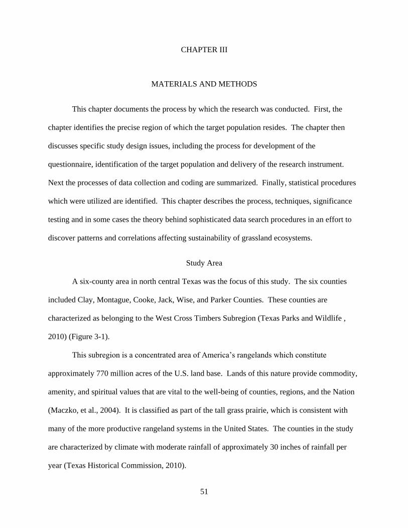
51
CHAPTER III
MATERIALS AND METHODS
This chapter documents the process by which the research was conducted. First, the
chapter identifies the precise region of which the target population resides. The chapter then
discusses specific study design issues, including the process for development of the
questionnaire, identification of the target population and delivery of the research instrument.
Next the processes of data collection and coding are summarized. Finally, statistical procedures
which were utilized are identified. This chapter describes the process, techniques, significance
testing and in some cases the theory behind sophisticated data search procedures in an effort to
discover patterns and correlations affecting sustainability of grassland ecosystems.
Study Area
A six-county area in north central Texas was the focus of this study. The six counties
included Clay, Montague, Cooke, Jack, Wise, and Parker Counties. These counties are
characterized as belonging to the West Cross Timbers Subregion (Texas Parks and Wildlife ,
2010) (Figure 3-1).
This subregion is a concentrated area of America‘s rangelands which constitute
approximately 770 million acres of the U.S. land base. Lands of this nature provide commodity,
amenity, and spiritual values that are vital to the well-being of counties, regions, and the Nation
(Maczko, et al., 2004). It is classified as part of the tall grass prairie, which is consistent with
many of the more productive rangeland systems in the United States. The counties in the study
are characterized by climate with moderate rainfall of approximately 30 inches of rainfall per
year (Texas Historical Commission, 2010).
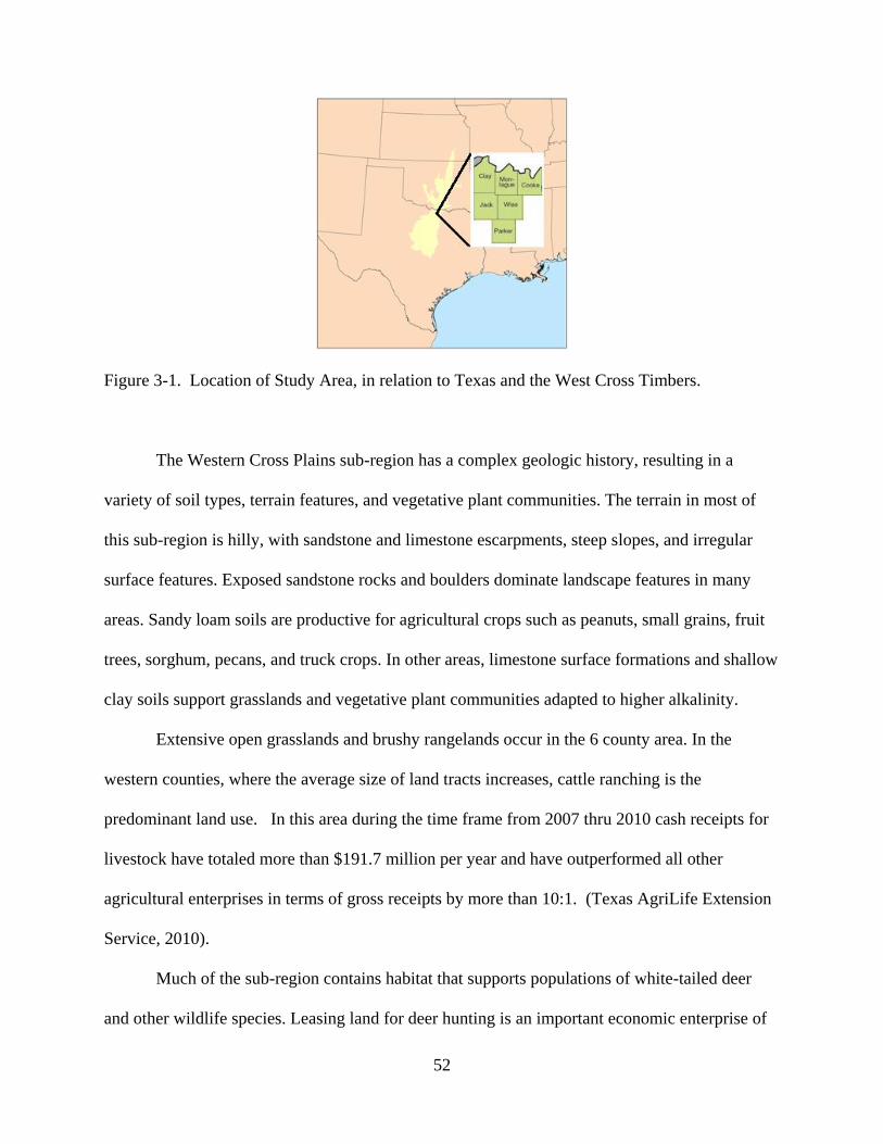
52
Figure 3-1. Location of Study Area, in relation to Texas and the West Cross Timbers.
The Western Cross Plains sub-region has a complex geologic history, resulting in a
variety of soil types, terrain features, and vegetative plant communities. The terrain in most of
this sub-region is hilly, with sandstone and limestone escarpments, steep slopes, and irregular
surface features. Exposed sandstone rocks and boulders dominate landscape features in many
areas. Sandy loam soils are productive for agricultural crops such as peanuts, small grains, fruit
trees, sorghum, pecans, and truck crops. In other areas, limestone surface formations and shallow
clay soils support grasslands and vegetative plant communities adapted to higher alkalinity.
Extensive open grasslands and brushy rangelands occur in the 6 county area. In the
western counties, where the average size of land tracts increases, cattle ranching is the
predominant land use. In this area during the time frame from 2007 thru 2010 cash receipts for
livestock have totaled more than $191.7 million per year and have outperformed all other
agricultural enterprises in terms of gross receipts by more than 10:1. (Texas AgriLife Extension
Service, 2010).
Much of the sub-region contains habitat that supports populations of white-tailed deer
and other wildlife species. Leasing land for deer hunting is an important economic enterprise of
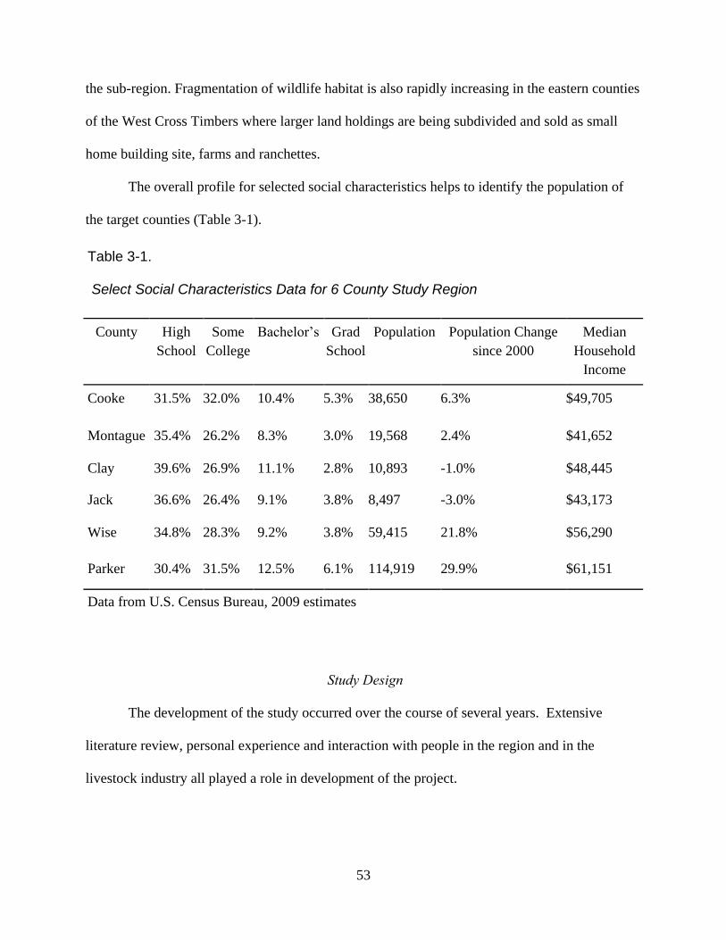
53
the sub-region. Fragmentation of wildlife habitat is also rapidly increasing in the eastern counties
of the West Cross Timbers where larger land holdings are being subdivided and sold as small
home building site, farms and ranchettes.
The overall profile for selected social characteristics helps to identify the population of
the target counties (Table 3-1).
Table 3-1.
Select Social Characteristics Data for 6 County Study Region
County High
School
Some
College
Bachelor‘s Grad
School
Population Population Change
since 2000
Median
Household
Income
Cooke 31.5% 32.0% 10.4% 5.3% 38,650 6.3% $49,705
Montague 35.4% 26.2% 8.3% 3.0% 19,568 2.4% $41,652
Clay 39.6% 26.9% 11.1% 2.8% 10,893 -1.0% $48,445
Jack 36.6% 26.4% 9.1% 3.8% 8,497 -3.0% $43,173
Wise 34.8% 28.3% 9.2% 3.8% 59,415 21.8% $56,290
Parker 30.4% 31.5% 12.5% 6.1% 114,919 29.9% $61,151
Data from U.S. Census Bureau, 2009 estimates
Study Design
The development of the study occurred over the course of several years. Extensive
literature review, personal experience and interaction with people in the region and in the
livestock industry all played a role in development of the project.
54
Questionnaire Development
Pilot Study
Initially, a preliminary study was conducted in the spring of 2009, designed to help
develop the livestock manager‘s survey. This questionnaire was developed based on information
reported in current peer-reviewed grazing management articles and range management text
books.
The instrument for this pilot study was focused on land managers in Cooke and
Montague Counties in north Texas, but it was not an attempt to get an all-inclusive list of range
managers in the study area. Instead, this preliminary study was given to range managers that
have a relationship with the researcher or with Texas AgriLife Extension in Cooke County.
Specifically, members of the Cooke County Farm Bureau Board of Directors (17 total), the
Cooke County Beef Cattle Improvement Association Board of Directors (10 total), and select
persons associated with Cooke and Montague County Farm Service Agencies (20 total). This
resulted in polling of 47 individuals. The response rate was 45%, with 21 surveys being
returned.
Data were collected in person and through the mail. Surveys were hand delivered. No
formal scientific method or procedure was used for contacting possible respondents to improve
response rate. Instead the response rate was dependent on affiliation of respondents with the
researcher. It is noteworthy that this collection method could skew the data collected. Once
again, a comprehensive scientific study was not the goal of the pilot study. The study was
implemented to improve the quality of the final survey instrument and to formalize some of the
analytic procedures that would ultimately be used. Study population was not random, nothing
more than procedural ―practice‖ and research refinement could be obtain from the data collected.
55
Focus Group
A Focus group was conducted during February of 2010. The focus group was made up
of key stakeholders from the north Texas cross timbers area. Identification of focus group
members occurred with the help of the Natural Resource Conservation Service‘s (NRCS)
management and the research team. Criteria for inclusion was management of a ranching
enterprise, which NRCS management or research team members perceive as superior for
ecosystem, economic or social outcomes. These perceived superior outcomes may have been
identified by received awards garnered by ranchers, or by physical evidence. Once identified,
selected focus group members were invited to participate by telephone, and then formally invited
by mailed invitation. It included 1 rangeland researcher, 2 rangeland educators, and 3 ranchers.
This focus group was conducted with the intent to more fully understand predominant whole-
ranch grazing management perceptions pertaining to economic, social, and ecological outcomes.
As suggested by Briske et al. (2008), this circumstantial evidence derived from successful
grazing managers experiences may be compared with experimental research to gain valuable
insight and develop a more robust approach to understanding and implementing successful
grazing management. Qualitative data collected from our focus group was documented and used
to develop questionnaires necessary for thorough assessment of whole-ranch management.
A summary of the focus group discussion was compiled and the information was used
along with the information gathered in the pilot survey to compile a second pilot survey. This
survey was sent to focus group participants. They were asked to evaluate the instrument. The
only suggestions that were received from their evaluation were in regards to typos and question
wording, rather than the substance or intent of the questions.
56
Target Population
Initially, the group to be targeted was native range livestock producers from Cooke,
Montague, Clay, Wise, Jack, and Parker counties in TX, who received benefits under the 2005-
2007 Livestock Disaster Program. This represented the most comprehensive, known listing of
cow/calf producers in the given area.
The request for the list was sent to Juan Garcia, acting Texas State Executive Director for
the USDA Farm Service Agency. The request was processed under the Freedom of Information
Act on Feb 9, 2009. At that time the request was determined to fall within the jurisdiction of the
Kansas City Admnistrative Services Branch of FSA and was reffered to them. The list was
received in spring of 2009. Because USDA limits compensation under government programs to
individuals with gross earnings under $250,000, the survey population may have omitted
managers with more available resources or those who were qualified but chose not to participate
in the government‘s disaster program. Therefore, it was decided to utilize information from the
tax appraisal district for each of the 6 counties identified earlier.
The final decision was made that the population to be evaluated would be defined as all
landowners in the Cooke, Jack, Montague, Wise, Parker, and Clay county areas with 500 acres of
native grass land with agricultural use property tax evaluations. The designation of 500 acres
was set because the objective of the research is to reconcile experimental studies and ―ranch-
scale‖ evidence. This criterion requires limiting survey population to include only those with
―ranch-scale‖ experience rather than ―hobby ranchers.‖
The list of the individuals, in the target population, was obtained by request from the
county appraisal districts of each respective county. Original lists included much duplication of
families or ranches due to ownership of multiple parcels of land with slight variations in listed
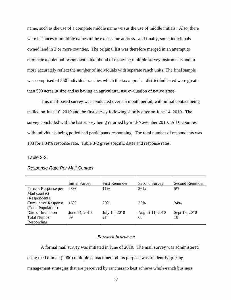
57
name, such as the use of a complete middle name versus the use of middle initials. Also, there
were instances of multiple names to the exact same address. and finally, some individuals
owned land in 2 or more counties. The original list was therefore merged in an attempt to
eliminate a potential respondent‘s likelihood of receiving multiple survey instruments and to
more accurately reflect the number of individuals with separate ranch units. The final sample
was comprised of 550 individual ranches which the tax appraisal district indicated were greater
than 500 acres in size and as having an agricultural use evaluation of native grass.
This mail-based survey was conducted over a 5 month period, with initial contact being
mailed on June 10, 2010 and the first survey following shortly after on June 14, 2010. The
survey concluded with the last survey being returned by mid-November 2010. All 6 counties
with individuals being polled had participants responding. The total number of respondents was
188 for a 34% response rate. Table 3-2 gives specific dates and response rates.
Table 3-2. Response Rate Per Mail Contact
Initial Survey
First Reminder
Second Survey
Second Reminder
Percent Response per
Mail Contact
(Respondents)
48% 11% 36% 5%
Cumulative Response
(Total Population)
16% 20% 32% 34%
Date of Invitation June 14, 2010 July 14, 2010 August 11, 2010 Sept 16, 2010
Total Number
Responding
89 21 68 10
Research Instrument
A formal mail survey was initiated in June of 2010. The mail survey was administered
using the Dillman (2000) multiple contact method. Its purpose was to identify grazing
management strategies that are perceived by ranchers to best achieve whole-ranch business
58
objectives and ecosystem enhancing practices for mid to tall-grass rangelands in the USA.
Surveys addressed the same issues as identified in the previous pilot survey and focus group
analysis: management philosophy; economic indicators; land health; management practices;
quality of life and cultural experiences, and personal characteristics.
Finally, non-response bias was tested. This was accomplished by sending a second, but
short non-response survey. Bias was determined by statistically significant differences in
demographic make-up of the two groups.
Questionnaire Design
The questionnaire (Appendix A) was an 8 ½ x 11 inch booklet printed front and back on
white paper. The instrument was 11 pages in length and had 5 sections. Page 1 was the cover;
page 2 was survey instructions; pages 3-4 were the first section, Management Philosophy; page
4-5 contained section 2, Economic Considerations; page 6-7 had section 3, Native Rangeland
Management; page 8-9 included section 4, Land Health. Section 5, Quality of Life, began on
page 9 and concluded on page 10. Finally, section 6, Personal Characteristics began on page 11.
The entire questionnaire consisted of 118 separate questions.
Questionnaire Implementation
Manager data were collected using a four-wave mailing (Dillman, 2000) multiple contact
method. A tracking code was included on all mailings, to facilitate follow up mailings. One
month after the initial mailing, a reminder post card was mailed to all potential respondents.
Responses were tracked over time. Four weeks after the reminder post card was mailed another
cover letter, questionnaire and business reply envelope was mailed to all non-respondents. One
more reminder post card was sent to all non-respondents.
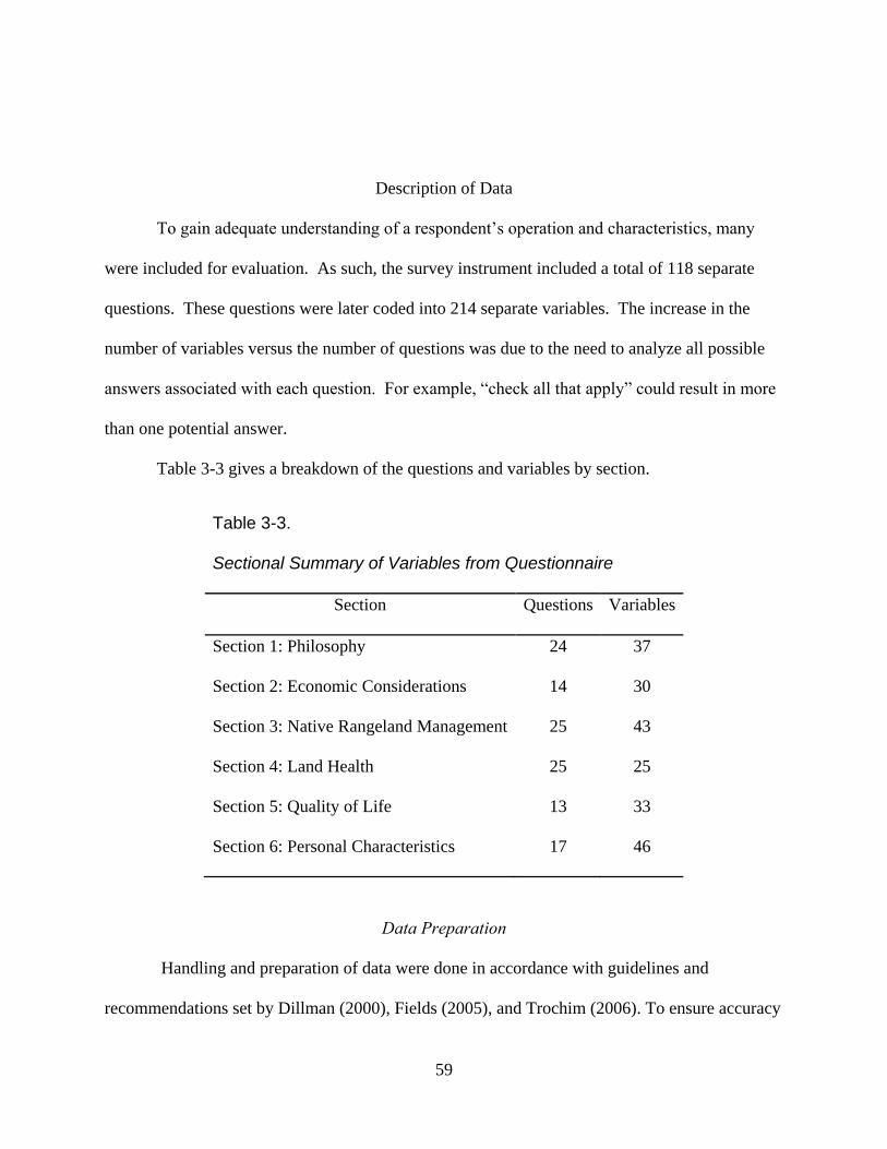
59
Description of Data
To gain adequate understanding of a respondent‘s operation and characteristics, many
were included for evaluation. As such, the survey instrument included a total of 118 separate
questions. These questions were later coded into 214 separate variables. The increase in the
number of variables versus the number of questions was due to the need to analyze all possible
answers associated with each question. For example, ―check all that apply‖ could result in more
than one potential answer.
Table 3-3 gives a breakdown of the questions and variables by section.
Table 3-3.
Sectional Summary of Variables from Questionnaire
Section Questions Variables
Section 1: Philosophy 24 37
Section 2: Economic Considerations 14 30
Section 3: Native Rangeland Management 25 43
Section 4: Land Health 25 25
Section 5: Quality of Life 13 33
Section 6: Personal Characteristics 17 46
Data Preparation
Handling and preparation of data were done in accordance with guidelines and
recommendations set by Dillman (2000), Fields (2005), and Trochim (2006). To ensure accuracy
60
during sampling, all surveys were coded with a unique letter and number sequence to allow for
documentation of respondent‘s return of the survey, either with a completed questionnaire or
with a refusal to reply.
Data were initially entered into a Microsoft Excel spreadsheet. Then, each of the 214
variables were entered into SPSS 18.0 and coded as numeric, given values, and identified as
ordinal, scale, or nominal. Variable names were given to all variables, based on the position it
occurred in the survey. The first number in the variable relates to the section in which it was
located. The second number relates to the question number on the survey. Further numbers
were assigned when individual questions required additional variable names, such as cases where
the question asked ―check all that apply‖, e.g. 3.3.1 or 6.14.5 etc.
Data Entry
Seven point Likert scale data was entered exactly as recorded by the respondent, with
numeric, ordered rankings of 1 through 7: 1 = strongly agreed; 2 = agree; 3 = somewhat agree;
4 = neutral; 5 = somewhat disagree; 6 = disagree; and 7 = strongly disagree. Section 4
included a 4 point Likert scale. These data were entered as ordered data, 1 through 4: 1 =
increased; 2 = remained constant; 3 = decreased; 4 = unknown. All other ordered data were
entered with the first listed category = 1 and sequentially increasing until all additional
categorical options were exhausted. These questions were found in Section 1, Question 5;
Section 3, Native Rangeland Management, Questions 1, 5, 6, and 7; Section 5, Quality of Life,
Question 2; and Section 6, Personal Characteristics, Questions 1, 5, 7, 8, and 17.
True/False data were coded as 1 = True, 2 = False
61
Other categorical questions were coded as yes/no dichotomous variables, with 0 = no and
1 = yes. These questions were found in Section 1, Questions 1, 2, 3, and 4; Section 2, Economic
Considerations, Question 1 and 2; Section 3, Native Rangeland Management, Questions 3 and 4;
Section 5, Quality of Life, Questions 1, 3, and 4 ; and Section 6, Personal Characteristics,
Questions 10, 11, and 12.
Finally, continuous data were entered with actual values. These included section 3,
Native Rangeland Management, Question 2; and Section 6, Personal Characteristics, Questions
2, 3, 4, 9, 13, 14, 15, and 16.
Missing values were coded as 99. Questions where the respondent marked ―DK‖,
indicating ―Don‘t Know‖, were coded as 98. Data were analyzed initially with SPSS (SPSS,
2009).
Statistical Analysis
Statistical analyses were conducted using a combination of statistical software. SPSS 18.0
(SPSS, 2009) was used whenever possible. When procedures called for methods not supported
by SPSS, statistical packages which were available in R-version 2.13.0 (R-2.13.0, 2011) software
was utilized. An analysis of descriptive statistics including N, mean, sum, standard deviation,
variance, range, minimum, maximum, standard error of the mean, kurtosis, kurtosis standard
error, skewness, and skewness standard error was conducted using SPSS.
Missing Data
The complexity of the desired analysis and the small size of the data set, made it
imperative to retain all cases available, therefore, missing data needed to be addressed. One
common solution is omission of variables or cases in the study with many instance of missing
data (Starkweather, 2011a).
62
There are numerous ways to deal with missing data. Wayman (2003) stated, ―It is
important to understand that once data are missing, it is impossible not to treat them –once data
are missing, any subsequent procedure with that data set represents a response in some form to
the missing data problem. As a result, there are many different methods of managing missing
data‖. Abrams (2007) suggested, ―If there are missing values for several cases on different
variables, omission of the variable or the case would lead to data being lost.‖ He then implied
that some form of analysis would be recommended to impute missing values. Imputation of
missing values can be done by several methods. According to Gelman and Hill (2006) the last
value could be carried forward, information from related observations could be used, indicator
variables for ―missingness‖ of categorical or continuous predictors is an option, or imputation
could be done based on logical rules. However, when more than just a ―trivial fraction‖ of data
contains missing information, it is preferred to use some form of random imputation.
Garson (2011e) recommends checking for data missing completely at random (MCAR)
versus missing at random (MAR). He states most often data is (MAR). Additionally he states,
―If data are MCAR, then the researcher may choose listwise or pairwise deletion of cases. If data
are not MCAR, missing values should be imputed.‖
MCAR can be confirmed by dividing respondents into those with and without missing
data, then using t-tests of mean differences on income, age, gender, and other key variables to
establish that the two groups do not differ significantly (Garson, 2011e). Therefore, an
independent t-test was used to check for differences between groups of respondents with missing
information and those without.
The random imputation approach was taken during this analysis. Variables and cases
were subjected to analysis by the R package ‗seqKnn‘ in version 2.13.0. This package estimates
missing values sequentially from the gene, that has least missing rate in microarray data, using
63
weighted mean of k nearest neighbors, where 1 row (case) is represented as one gene (Kim et al.,
2004).
While much of the literature implies the use of ‗seqKNN‘ with the use of missing data
concerning gene expression (Hastie et al., 1999; Kim et al., 2004; Kim et al., 2009), the package
‗seqKNN‘ uses Euclidean distance to impute missing data and is applicable for many situations.
This method is quite simple in principle but is effective and often preferred over other methods
Nearest neighbors are records that have similar completed data patterns; the average of the k-
nearest neighbor‘s completed data are used to impute the value for a variable that is missing its
value (where k can be set by the analyst or R user) (Kim and Yi, 2008; Starkweather, 2010b).
Hastie, et al. (1999) have shown choosing k ranging from 5 to 10 is adequate.
The advantage of the knn approach is that it missing data only depends on the observed
data. This package assumes data are missing at random. This then allows the knn approach to
take advantage of multivariate relationships in the completed data. The disadvantage of this
approach is it does not include a component to model random variation; consequently
uncertainty in the imputed value is underestimated (Starkweather 2011a).
Imputation of missing values was conducted using package ‗SeqKnn‘ in R version 2.13.0
(Kim and Yi, 2009). Imputed values were used throughout all analyses during inferential
statistical procedures. For the purposes of these analyses, 5 was chosen as k.
Rounding
Data imputed with the R package ‗SeqKnn‘ was not necessarily a whole number. In order to
have these values fit into the ordered and nominal data categories insuring consistency with other
data, these values were rounded to the nearest whole number. This task was accomplished using
the ‗round‘ function which is available with the ‗base‘ package of R version 2.13.0. (R-2.13.0,
2011).
64
Internal Consistency
Sections 2, 4, and 5 of the questionnaire were designed to gather information about ranch
level indicators to assess the degree of sustainability associated with economic, ecological and
social elements of rangeland management as indicated by literature (West and Herrick, 2003;
Maczko et al., 2004; Heitschmidt et al., 2004). These sections were used for creation of three
indices which implicate the degree of sustainability which can be assigned to each respondent‘s
ranch concerning each of the three sustainability elements.
One of the stated objectives of this research is to assess the impact of grazing
management philosophy, land management practices, and respondent‘s personal characteristics
on grassland sustainability (which the survey attempts to capture in Sections 1, 3, and 6). There
must be a way to measure the impact. Creating a metric from responses to Sections 2, 3, and 5
will allow for these critical comparisons. When creating the metric, which referred to as the
sustainability indices,‖ the extent to which questions within each section assessed the same
characteristic needed to be measured to reduce the number of ambiguous variables.
Also, there is a need to demonstrate the testing instrument is reliable. Internal
consistency is a gauge of the relationship between each item and each other item. It may help
researchers interpret data and predict the limits of the relationship among variables (Howell et
al., 2005).
Furthermore, Garson (2011a) states that indices are sets of items which are thought to
measure a latent variable. Items in an index will normally be more intercorrelated with each
other than with other items. Cronbach's alpha is a common test of whether items are sufficiently
interrelated to justify their combination in an index (Starkweather, 2011b) and is a useful
coefficient for assessing internal consistency (Cronbach, 1951; Bland and Altman, 1997).
Likewise, when attempting to measure a construct with multiple indicator variables, as done
65
here, it must be demonstrated that the items measure the same thing because lack of
unidimensionality is a form of measurement error (Garson, 2011c). For this reasoning, internal
consistency of variables was very important to the sustainability sections.
As a result, the first step in creating sustainability indices for inferential purposes was the
identification of variables which maximized Cronbach‘s Alpha coefficient. This analysis was
conducted using SPSS 18.0. This procedure was much the same as those preformed by Doll and
Jackson (2009), in their effort to understand farmer attitudes.
Derived Scales
Scaling is the branch of measurement that measures what is originally an ―unmeasurable"
construct. Trochim (2006) gives examples of these constructs like authoritarianism and self
esteem. In the context of this study the ―unmeasurable‖ construct is sustainability.
Trochim, (2006) also acknowledges, ―On some scales, you will have items that are
reversed in meaning from the overall direction of the scale. These are called reversal items. You
will need to reverse the response value for each of these items before summing for the total. That
is, if the respondent gave a 1, you make it a 5; if they gave a 2 you make it a 4; 3 = 3; 4 = 2; and,
5 = 1.‖ This is the case with some of the variables to be included in the sustainability indices.
All variables were transformed so that scale scores would align consistently within each index.
A summation of the selected variables from section 2, ―Economic Considerations‖ was
identified as a good metric for sustainability of economic indicators. Scale scores were
calculated by simply adding each respondents selection of 1 through 7 from Likert scale
information; the lower the sum, the greater the sustainability.
The Likert scale for section 4 ―Land Health‖ was a 4 point scale. Variables were
measured on the scale as 1= increase; 2 = constant; 3 = decrease; and 4= unknown. Some of the
66
variables would tend toward sustainability if they were increasing, some if they were decreasing.
For example, an increase in brush does not align with sustainable rangeland indicators (West and
Herrick, 2003), while an increase in wildlife would. Transformation of values for increasing and
decreasing was applied to some variables in the index so all were consistent with respect to
sustainability. Ultimately, 3 was a value indicating greater sustainability, 1 lesser; 4 (unknown
categories were replaced using software available in the R environment, package ‗seqKNN‘).
In section 5, ―Quality of Life‖ all variables included in the sustainability index were 7
point Likert scale questions. Simple summation of respondent answers was used for creation of
this Social Sustainability Index. All questions aligned so that the lower the score, the more
sustainable the case.
Economic Considerations
Prior to maximizing for Cronbach‘s alpha coefficient, transformations to select variables
were necessary. Preliminary analysis may reveal inconvenient coding schemes or coding errors,
or data transformations may be required in order to expose the true relationship between
variables (SPSS, 2009a).
Section 2, Economic Considerations, originally was composed of 14 questions and 30
variables. The last questions, 2.1 and 2.2 were questions asking the respondent to ―check all that
apply.‖ These were originally coded into SPSS with each possible response being a single,
dichotomous, yes/no variable, resulting in 18 total variables. When analyzing for Cronbach‘s
alpha using SPSS 18.0, without transformation of these variables, the determinant of the
covariance matrix was zero. Therefore, statistics based on its inverse matrix could not be
computed. This causes questionable output in SPSS 18.
67
Transformation of the problem variables to a single categorical variable was
accomplished by simply adding the number of selections with a ―yes‖ per question, per
respondent. The questions were, 2.1:―I measure economic success on the ranch by: (Check all
that apply)‖ and 2.2: ―My ranch uses diversification of enterprises to reduce risk or increase
income. If yes, I diversify by: (Check all that apply)‖.
Question 2.1 became the number of economic measures used to detect economic success
and 2.2 became the number of diversified enterprises used on the respondent‘s ranch. It was
theorized that the greater the number of measures for economic success, or the greater the
diversification, the more sustainable the operation may be. The end result was a reduction of 30
original variables to 14, one per question. These were evaluated for internal consistency.
SPSS version 18.0 was used to evaluate the Cronbach‘s alpha coefficient. The analysis
was computed consecutively with reduction of variables as suggested by the item to correlation
score, until Cronbach‘s Alpha Coefficient was maximized. Desired outcome to variables as
unidimensional for confirmatory purposes was set at a critical value of alpha as 0.7(α = .7)
(Nunnaly & Bernstein, 1994; Starkweather, 2011b; Garson, 2011c).
Land Health
Section 4, ―Land Health‖, was comprised of 25 ordered questions which resulted in an
equal number of 25 ordered variables. All variables were evaluated for internal consistency
using SPSS version 18.0 and evaluating for the Cronbach's alpha coefficient greater than 0.7.
SPSS version 18.0 was used to evaluate the Cronbach‘s alpha coefficient. The analysis was
computed consecutively with reduction of variables as suggested by the item to correlation score.
Quality of Life
68
Finally, Section 5, ―Quality of Life‖, was evaluated for internal consistency. All thirty-
three variables were analyzed . SPSS version 18.0 was used to evaluate the Cronbach‘s alpha
coefficient. The analysis was computed consecutively with reduction of variables as suggested
by the item to correlation score, until Cronbach‘s Alpha Coefficient was maximized.
Optimal Scaling
Nominal and ordinal variables, relative to interval variables, are less amenable to
analysis. Garson (2011a) states that retaining categorical data when utilizing inferential
statistical procedures could lead to the presence of empty cells and can undermine traditional
regression. He also reports, the presence of empty factor cells in the model will undermine the
validity of the ensuing goodness of fit tests and model validity will be uncertain. To deal with
this problem, nominal and ordinal variables can be converted to interval variables through one of
several techniques known as optimal scaling (Moss, 2008). Certain statistical software packages
such have been developed to implement data conversion by optimal scaling (SPSS Inc, 2009b;
de Leeuw and Mair, 2010).
The optimal scaling process turns qualitative variables into quantitative. How this occurs
is dependent on the data set and the criterion for optimization. Various methods exist for creation
of optimality. These include discrimination among objects, maximization of homogeneity or
internal consistency among variables, making pairwise relationships as linear as possible,
maximization of variance accounted for (in the analysis of interdependence), and transformations
toward additivity, maximization of r2, canonical correlation, and the ratio of between to total
dispersion; in the optimal scaling process an appropriate quantification level has to be chosen
(Meulman, J., 1988)
69
Mair and de Leeuw (2010) describe a general framework for multivariate analysis with
optimal scaling whereby, multivariate data are collected into a multivariable ―aspect‖. This
aspect of a multivariable is a function that is used to measure how well the multivariable satisfies
some criterion. Two different families of aspects exist: non-correlational and correlational. It is
quite possible that the two will give the same transformations. If the goal is to achieve
bilinearization, then the non-correlational aspect, LINEALS, should be chosen. ―A function of
two variables is bilinear if it is linear with respect to each of its variables. The simplest example
is f(x, y) = x y” (Weisstein, 2011).
Many parametric statistical routines, like regression assume that the effects of each
variable on the target are linear; if the effects are non-linear, transformation of data are
recommended (Field, 2005). Therefore, because binearization was desirable, the R package
‗aspect‘ and the non-correlational aspect, LINEALS was chosen for use in optimal scaling of
data obtained during the study.
When using the R package ‗aspect‘, the LINEALS function makes transformations of the
variables such that all bivariate regressions are exactly linear. This is a function combining
elements of two vector spaces (consisting of an ordered collection of numbers) to yield an
element of a third vector space that is linear in each of its arguments. In the case of LINEALS
this is rjl of the Pearson correlation matrix and the Pearson correlation ratio. A matrix of these
quantifications is available in the R output. After optimization, asymptotic tests and estimates
can still be used on the transformed data (de Leeuw and Mair, 2010)
To assess the relative success of the imputation, part of the output is characterized as
―loss‖. Loss of information occurs when discretizing (grouping) variables and then performing
optimal scaling (Mair and de Leeuw, 2010). They do not quantify loss, but simply state, ―the
lower, the better‖. They explain further by reporting that eventually, the value of the LINEALS
70
loss function can be used as total discrepancy index or criteria for determining acceptability of
cases. Smaller loss equates to more closely achieving bilinearizability a discrepancy index of 0
would be perfect. This is not realistic for real-life applications. In fact, de Leeuw et al. (1999)
mention that we may be able to successfully approximate bilinearizability in ordinal data but it is
very unlikely in purely nominal variables. Still, minimization using LINEALS, even with
nominal data leads to a lower discrepancy compared to other optimal scaling techniques.
Therefore, if the aim is to achieve bilinearization, LINEALS should be considered (Mair and de
Leeuw, 2010).
Continuous variables were not optimally scaled. Instead these were removed from the
data set prior to optimization. The discretized variables and the continuous variables were then
recombined into a data set and used for further the analysis. Handling of the continuous data in
this manner is similar to ordinal regression as carried out by SPSS (SPSS Inc, 2009b).
Principal Component Analysis
With 214 original variables, it was necessary to methodically select a subset of variables,
based on which original variables have the highest correlations with the principal component
factors within each section of the survey. The subsets retain only those variables with
meaningful relationships to the structure of the survey (Garson, 2011b).
When attempting to measure a construct with multiple predictors, the items must measure
the same thing or measurement error will be present. Also, measurement error would increase
standard error in subsequent regression analysis (Garson, 2011c). Because of this, some form of
variable reduction must occur. This can be accomplished with principal component analysis
(PCA), which is a preferred method for data reduction, (StatSoft Inc., 2011).
71
Traditional PCA is a variable reduction technique which maximizes the amount of
variance accounted for in the observed variables by identifying a smaller group of variables
called components (Starkweather, 2010a).
Principle component analysis was used as a means of identifying a subset of variables
based on which original variables have the highest correlation with the principal components,
also known as component loadings (Garson, 2011b; StatSoft Inc., 2011). The analysis was run
using SPSS 18.0. Data was loaded into SPSS after optimal scaling. Sections, 1, 3, and 6 were
analyzed with PCA separately. An extra, fourth PCA was also conducted using variables that
did not help to maximize Crobach‘s Alpha and were therefore not used in resulting sustainability
indexes.
Selection of Components
According to Field (2005) a scree plot should be used to determine number of factors in
instances where the number of variables is between 30 and 250, which is consistent with the data
derived from the questionnaire. However, he also explains that the sample size needs to be
greater than 200, which is not consistent with this study.
Another method beginning to gain popularity for determining the number of principal
components is the use of ―Parallel Engine Analysis‖. This analysis is based on parameters
provided by the researcher. It calculates eigenvalues from randomly generated correlation
matrices. These can be then compared with eigenvalues extracted from the researcher's dataset.
The number of factors to retain will be the number of eigenvalues that are larger than the
corresponding random eigenvalues (Horn, 1965). A parallel analysis engine to aid determining
number of factors to retain is available online at: http://ires.ku.edu/~smishra/parallelengine.htm/.
The engine utilizes a SAS-based code written by O'Connor (2000).
72
Scree plot analysis is extremely reliable, even compared to parallel engine analysis (Patil
et al., 2007). A scree plot is a graphical method first proposed by Cattell (1966). The object is to
plot the eigenvalues for each additional component and connect them with a line. As the amount
of variance explained in each component decreases, the line will level off to the right of the plot.
To the right of this point, presumably, you find only meaningless components. The problem is
that this techinque is very subjective (Turner, 1988).
Still a third criterion is Kaiser‘s criterion, simply stated this is retaining all components
with eigenvalues greater than 1 (Field, 2005). Therefore, an approach using more than one
technique is preferred to a single approach for factor selection. This multiple approach, reduces
subjectivity yet allows for greater discernment by the researcher (Patil et al., 2007).
This study followed those guidelines and determined the number of principle components
to extract by a combined analysis using both Parallel Engine Analysis and Scree Plot Analysis
and additionally, Kaiser‘s criterion. Determination of the number of components to be used was
done initially, with no rotation procedure applied to the principle component analysis.
Rotation
The goal of rotating components is to a determine pattern of loadings identifying the
variables of interest. After considering various rotation strategies, Varimax rotaion was
selected. If fit best with the purpose of the study. The goal is to maximize the variance
(variability) of the "new" variable (factor), while minimizing the variance around the new
variable. This should obtain a pattern of loadings on each factor that is as diverse as possible,
lending itself to easier interpretation (StatSoft, 2011; Field, 2005).
Communalities
Communality is the squared multiple correlation for the variable as dependent using the
factors as predictors. Generally, they help to identify the measured variables for which the factor
73
analysis is working best. Likewise, low communalities may indicate that a predictor is not
working well and should be removed from the model. However, this is not always necessarily
so. Communalities must be interpreted in relation to the interpretability of the
factors/components. A communality of 0.75, which seems high, could actually be meaningless if
the component is not interpretable. On the other hand, a low communality may be meaningful if
it contributes to a well defined factor. Therefore, what is most important, more so than the actual
value, is the extent to which it contributes to the interpretation of the factor (Garson, 2011b).
Communalities are reported in this section of the results, so as to not lose sight of that fact, and
to aid in interpretation of variables.
Component Identification
Once the number of components, to be accepted as relevant is determined, component
loadings must be interpreted. Interpretation involves selecting variables which contribute to each
component‘s identity. There is some subjectivity involved when interpreting component
loadings. Various researches follow different rules of thumb. In confirmatory factor analysis, as
opposed to PCA, loadings should be 0.7 or higher to confirm that independent variables
identified a priori are represented by a particular factor. Reasoning is such that the 0.7 level
corresponds to about half of the variance in the indicator being explained by the factor. With
many data sets, the .7 standard is a high one and often data cannot meet this criterion. Often,
especially for exploratory purposes (PCA), researchers will use a lower level such as .4 for the
central factor and .25 for other factors (Raubenheimer, 2004). One example, Hair et al. (1998),
call loadings above 0.6 "high" and those below 0.4 "low". Factor/component loadings must be
interpreted in the light of theory, not by arbitrary cutoff levels (Garson, 2011b).
74
For the purpose of this study, loading equal to, or more extreme than + or - 0.6 are
described as high; loadings (both positive and negative between 0.6 and 0.4 are considered
moderate, and those less than + or – 0.4 are considered low.
Sampling Adequacy and Bartlett’s Test
Recommended procedures for accepting that the PCA has yielded reliable factors are a
check of Kaiser-Meyer-Olkin (KMO) measure of sampling adequacy and Bartlett‘s test of
sphericity. Kaiser (1974) recommends accepting values greater than 0.5. If values are found to
be lower, then rethinking which variables to include or collection more data may be a good idea
(Field, 2005).
Bartlettt‘s Test of sphericity tests the null hypothesis that the original correlation matrix
is an identity matrix. A significant result (p < .05) indicates the matrix is not an identity matrix,
and thus factor analysis would be appropriate (Field, 2005).
Bayesian Model Averaging
Bayesian model averaging (BMA) is a robust statistical technique which was useful for
selecting regression models (Raftery, 1995). It is the most appropriate model for comparison and
model fit statistics (Schwarz, 1978; Moore 2008). The BMA package/library (Raftery et al.,
2011) was used to select variables, as predictors for input into ordinary least squares regression.
These variables originated from Sections 1, 3, 6, and also included the variables from Sections 2,
4, and 5 which did not become part of the sustainability indices. These potential sustainability
predictors addressed respondents land management philosophy, native rangeland management
practices, and personal characteristics.
Specifically, the ―bicreg‖ function was used. This function accounts for the model
uncertainty, which is inherent in the variable selection process. It does this by first selecting
75
models that are likely to be the best, using ―approximate posterior model probability.‖ This
means finding the post regression probability that each variable is non-zero (Raftery et al., 2011).
It then averages variables, over the best models in the model class (Raftery, 1995; Raftery et al.,
2011).
This function is capable of selecting the best set of predictor variables for a linear
prediction model by building a normal curve distribution of how frequently a predictor is coming
up in a significant model. The model with the best fit is determined by the model with the
largest posterior probability and the lowest Bayesian information criterion (BIC) (Starkweather,
2011d). When estimating model parameters, it is possible to ―overfit‖, or superficially improve
the outcome, by continually adding additional parameters. This method of model selection
protects against the possibility of ―overfitting‖ by introducing a penalty for additional parameters
as opposed to simply maximizing for the amount of variance explained (McQuarrie, 1998).
To determine predictors impact on the sustainability indexes created from sections 2, 4,
and 5, impact was assessed from each set of predictors (variables) in section 1, 3, 6 and ―other
variables‖. Whereas, the sustainability index from section 2 becomes the first dependent
variable, all variables identified in prior PCA computations are then inputted into the ―bicreg‖
function using the BMA package in R version 2.13.0. The same holds true for section 4, and
then section 5. This necessarily means that 3 separate analyses must be run, one for each
dependent variable: the sustainability indices. Output indicated which variables should be
inserted into ordinary least squares regression. The variables which have been identified as
returning the best model was accepted (Raftery, 1995).
Hierarchical Regression Analysis
76
Multiple regression analysis was employed to account for the variance in the derived
sustainability indexes (sections 2, 4 and 5) based on predictors which were indicative of
respondents land philosophy, land management, or personal characteristics (sections 1, 3, and 6).
The goal is to gain insight concerning the amount of variance explained by the independent
variables identified through BMA, which is the most appropriate model for comparison and
model fit statistics (Schwarz, 1978).
In order to minimize predictors being selected purely by chance, hierarchical regression
analysis, a specific form of ordinary least squares, multiple regression analysis, was chosen as a
means of relating management philosophy, native rangeland management, and personal
characteristics to the sustainability indexes of economic considerations, land health, and quality
of life. Hierarchical regression predictors are entered into the analysis one block at a time, with
the researcher, not the computer, determines the order of entry of the variables. F-tests are used
to compute the significance of each added variable (or set of variables) to the explanation
reflected in R-square. The order they are entered should be selected based on past work (Field,
2005). Known predictors should be entered first, also known as covariates; followed by new
predictors, together or one at a time. Distinction between a covariate and a predictor is often
simply a matter of semantics (Starkweather, 2011c). The reason for the use of hierarchical
regression and the use of predictor entry in blocks is that this method isolates the effects caused
by specific variables in terms of both the predictive model and the relative contribution of
variables in each block. Essentially, variables that are conceptually linked to each other were
entered together in a block. Those variables which literature identified as most important were
entered first, while those which were more abstract concerning their role as a predictor, were
entered later.
77
After the regression analysis, the relative predictive importance of the independent
variables will be established by comparing beta weights. All predictor and dependent variables
were interval due to the optimal scaling process that was employed earlier in the analysis. This
analysis was conducted using SPSS 18.0.
Assumptions
Garson (2011c) explains that all statistical procedures have underlying assumptions.
Sometimes violations of these assumptions can be tolerated without changing substantive
research conclusions. In other cases, violation of assumptions is critical to meaningful research.
Every effort was made to adhere to relevant assumptions in order to assure the ability to draw
accurate conclusions.
Error was checked for normal distribution, using histograms and (P-P) plots.
Residual analysis was undertaken to check for lack of homoscedasticity and presence of
outliers, ensuring stability across the accepted model.
Multicollinearity was assessed to ensure that it is not present. Correlations were visually
assessed; VIF and Tolerance test were employed.
Robust techniques were employed to ensure that all data would fit with linearity
assumption (see section on optimal scaling).
Leaving variables out of the model when literature suggests they should be included is a
serious deviation from data assumptions. When constructing the most parsimonious
model, literature was has implicated independent variables of importance far beyond
those in the model. The regression model is, in part, an attempt to discern which
areas/variables are, in fact the most important for obtain sustainable rangeland
production.
Cross Validation
Careful application of multiple regression methods requires that the regression weights be
cross-validated on a different population (Stockburger, 2006). Field (2005) explains cross
78
validation as a useful tool to identify if the model derived from the study can be used to predict
the outcome in a different sample. Two methods can be used to do this: Shrinkage and Data
Splitting.
Shrinkage
The manner in which regression weights are computed guarantee that they will provide
an optimal fit with respect to the least square criterion for the existing set of data. Prediction
using a different data set leads to regression weights that are no longer optimal. This loss in
predictive power is referred to as shrinkage (Stockburger, 2006).
In SPSS adjusted R2 indicates shrinkage when variance is applied to other populations,
while R2 explains the variance in Y accounted for from the sample in the study. SPSS uses
Wherry‘s formula to derive at the adjusted R2. A much better indication of cross validation is
Steins‘s formula (Yin and Fan, 2001). Because of this fact, all adjusted R2 were recalculated by
hand then inserted in place of Wherry‘s formula for the most parsimonious block of the
hierarchical regression analysis. Whereas, Stein‘s formula is as follows, where n = number of
cases, and k is the number of predictors:
adjusted R2 = 1 – [(n – 1/n – k – 1) (n - 2/n – k – 2) (n + 1/n)] (1 – R
2)
Data Splitting
Data splitting is a good technique, but Field (2005) explains that researchers rarely have
enough cases t make splitting the data set practical. The procedure would be simply splitting the
cases in the study, computing a regression equation on two halves and comparing the results.
An alternative cross-validation method to simple data splitting is K-fold cross-validation.
With this method k – folds are randomly removed from the data set. (Starkweather, 2011e) The
original data set is randomly divided into K subsamples. A single subsample is retained as the
79
validation data for testing the model, and the remaining K − 1 subsamples are used as training
data. The number of folds selected (K) determine the number of times the cross-validation
process is repeaed (Moore, 2008).
Software provided by R version 12.13.0. package ‗DAAG‘ and the function ―CVlm‖
perform K-fold cross-validation analysis (Maindonald, 2011). This function gives internal and
cross-validation measures of predictive accuracy for multiple linear regressions. Therefore, it
was used in all cross-validation statistical procedures in this study.
Non-Response Bias Survey
Using SPSS 18.0, non-respondents returning the non-response bias questionnaire were
evaluated for differences in demographics, grazing patterns, and source used to obtain
management information (Appendix B).
80
CHAPTER IV
RESULTS
Chapter 4 provides the results of the study. It is divided into 3 parts. First, results
concerning the response rate and related agricultural statistics concerning the amount of land
from the six counties polled were discussed. Next and overview of the descriptive statistics is
given for sections 1, 2, 3, 4, and 5. A question by question description of section 6, ―Personal
Characteristics‖ is given. Finally, results from each of nine statistical procedures are given.
Seven of these procedures lead up to hierarchical regression analysis. After the regression,
results from the non-response bias survey are given.
Study Implementation
Of the 188 respondents, 124 indicated that they managed livestock on native rangeland
and went on to answer most questions in the survey. The remaining 64 respondent indicated that
they either did not own native rangeland, that they did not manage livestock on their land, or that
they simply lacked the knowledge of the land to answer the survey. Essentially, when
discounting the 64 unintentionally sampled respondents who indicated they were unable to
complete the questionnaire because they did not fit the target population, the total population
would have been 486. With 124 responding from this population, response rate would be 25.5%.
While this response rate is not ideal, it is in line with other studies seeking the opinion of
agricultural producers. Greiner et al. (2008) conducted a survey of farmer‘s motivations, polling
685 producers. They were able to gather 114 responses, or 16.6%. Similarly, Sydoravych and
Wossink (2008) polled a mixed group of agricultural producers, scientists and agriculture
industry employees; of that group they were only able to get a response rate of 25%. They
―believed that response rate was adequate, given no reward was offered‖. It is possible that
81
agriculture industry professionals, especially those in production agriculture are extremely
adverse to disclosure of personal information and perceptions.
Respondents with acreage completely within the 6 county area were in control of a total
of 327,017 acres, ranging from the smallest acreage of around 80 acres, to the largest ranch
comprising 18,000 acres. The area represented by respondents is approximately 13.65 % of the
acreage in pasture and rangeland in the 6 counties. When including respondents with acreage
outside of the 6 county area, the total number of acres being represented were 358,717. USDA
only reports the single category ―pasture and rangeland‖ and there is no single category
recognized as only ―rangeland‖. The term ―pasture‖ would include all types of improved and
introduced grasses such as bermudagrass (Cynodon dactylon), kleingrass (Panicum coloratum),
and improved bluestems (Bothriochloa ischaemum and Bothriochloa bladhii) (Table 4-1). The
first question in the survey asks perspective respondents, ―Do you own and/or manage native
rangeland that is utilized for livestock grazing?‖ If the answer was ―No‖, the potential
respondent was asked to ―Please stop here and return questionnaire in the attached postage-paid
envelope.‖ No was selected by 64 of the respondents as indicated earlier.
Descriptive Statistics
Because of its complex, muti-dimensional nature, agricultural sustainability is most often
assessed using numerous indicators, (Sydorovych and Wossink, 2008). This fact is reflected by
the large number of questions and variables included in the survey. Because of this each variable
will not be discussed by itself. Appendix C records the descriptive statistics for each variable. A
brief discussion concerning general characteristics of each section will follow.
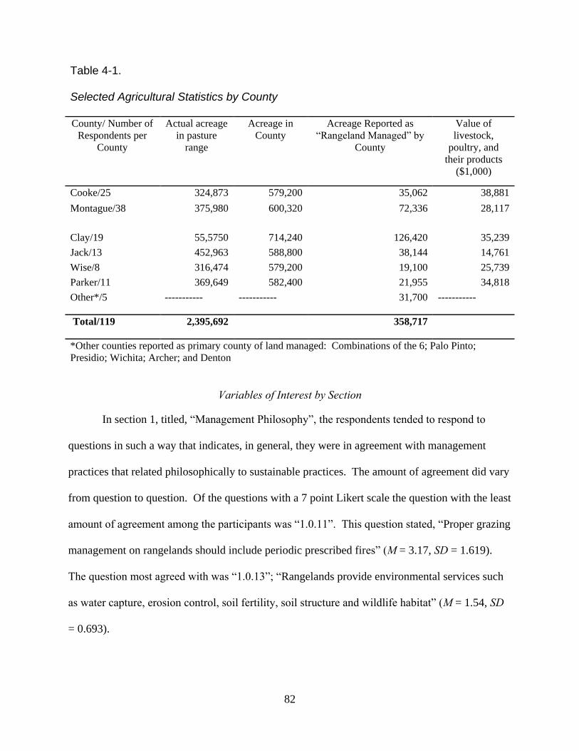
82
Table 4-1. Selected Agricultural Statistics by County County/ Number of
Respondents per
County
Actual acreage
in pasture
range
Acreage in
County
Acreage Reported as
―Rangeland Managed‖ by
County
Value of
livestock,
poultry, and
their products
($1,000)
Cooke/25 324,873 579,200 35,062 38,881
Montague/38 375,980 600,320 72,336 28,117
Clay/19 55,5750 714,240 126,420 35,239
Jack/13 452,963 588,800 38,144 14,761
Wise/8 316,474 579,200 19,100 25,739
Parker/11 369,649 582,400 21,955 34,818
Other*/5 ----------- ----------- 31,700 -----------
Total/119 2,395,692 358,717
*Other counties reported as primary county of land managed: Combinations of the 6; Palo Pinto;
Presidio; Wichita; Archer; and Denton
Variables of Interest by Section
In section 1, titled, ―Management Philosophy‖, the respondents tended to respond to
questions in such a way that indicates, in general, they were in agreement with management
practices that related philosophically to sustainable practices. The amount of agreement did vary
from question to question. Of the questions with a 7 point Likert scale the question with the least
amount of agreement among the participants was ―1.0.11‖. This question stated, ―Proper grazing
management on rangelands should include periodic prescribed fires‖ (M = 3.17, SD = 1.619).
The question most agreed with was ―1.0.13‖; ―Rangelands provide environmental services such
as water capture, erosion control, soil fertility, soil structure and wildlife habitat‖ (M = 1.54, SD
= 0.693).
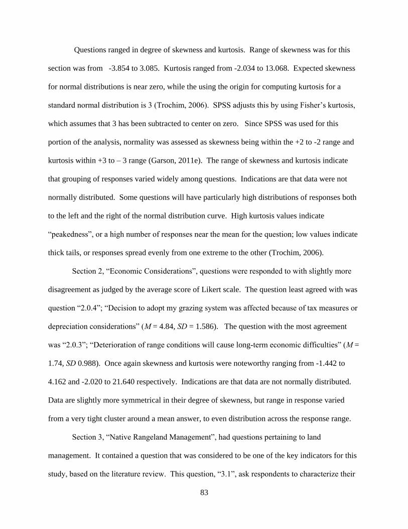
83
Questions ranged in degree of skewness and kurtosis. Range of skewness was for this
section was from -3.854 to 3.085. Kurtosis ranged from -2.034 to 13.068. Expected skewness
for normal distributions is near zero, while the using the origin for computing kurtosis for a
standard normal distribution is 3 (Trochim, 2006). SPSS adjusts this by using Fisher‘s kurtosis,
which assumes that 3 has been subtracted to center on zero. Since SPSS was used for this
portion of the analysis, normality was assessed as skewness being within the +2 to -2 range and
kurtosis within +3 to – 3 range (Garson, 2011e). The range of skewness and kurtosis indicate
that grouping of responses varied widely among questions. Indications are that data were not
normally distributed. Some questions will have particularly high distributions of responses both
to the left and the right of the normal distribution curve. High kurtosis values indicate
―peakedness‖, or a high number of responses near the mean for the question; low values indicate
thick tails, or responses spread evenly from one extreme to the other (Trochim, 2006).
Section 2, ―Economic Considerations‖, questions were responded to with slightly more
disagreement as judged by the average score of Likert scale. The question least agreed with was
question ―2.0.4‖; ―Decision to adopt my grazing system was affected because of tax measures or
depreciation considerations‖ (M = 4.84, SD = 1.586). The question with the most agreement
was ―2.0.3‖; ―Deterioration of range conditions will cause long-term economic difficulties‖ (M =
1.74, SD 0.988). Once again skewness and kurtosis were noteworthy ranging from -1.442 to
4.162 and -2.020 to 21.640 respectively. Indications are that data are not normally distributed.
Data are slightly more symmetrical in their degree of skewness, but range in response varied
from a very tight cluster around a mean answer, to even distribution across the response range.
Section 3, ―Native Rangeland Management‖, had questions pertaining to land
management. It contained a question that was considered to be one of the key indicators for this
study, based on the literature review. This question, ―3.1‖, ask respondents to characterize their
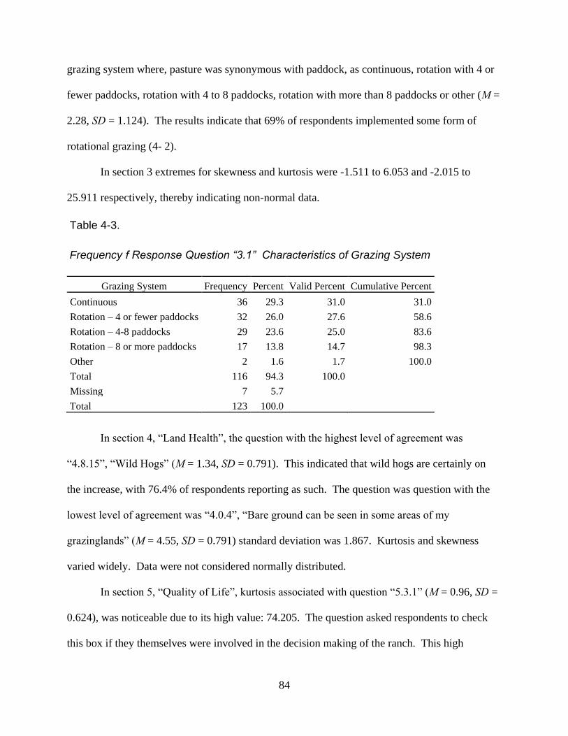
84
grazing system where, pasture was synonymous with paddock, as continuous, rotation with 4 or
fewer paddocks, rotation with 4 to 8 paddocks, rotation with more than 8 paddocks or other (M =
2.28, SD = 1.124). The results indicate that 69% of respondents implemented some form of
rotational grazing (4- 2).
In section 3 extremes for skewness and kurtosis were -1.511 to 6.053 and -2.015 to
25.911 respectively, thereby indicating non-normal data.
Table 4-3.
Frequency f Response Question “3.1” Characteristics of Grazing System
Grazing System Frequency Percent Valid Percent Cumulative Percent
Continuous 36 29.3 31.0 31.0
Rotation – 4 or fewer paddocks 32 26.0 27.6 58.6
Rotation – 4-8 paddocks 29 23.6 25.0 83.6
Rotation – 8 or more paddocks 17 13.8 14.7 98.3
Other 2 1.6 1.7 100.0
Total 116 94.3 100.0
Missing 7 5.7
Total 123 100.0
In section 4, ―Land Health‖, the question with the highest level of agreement was
―4.8.15‖, ―Wild Hogs‖ (M = 1.34, SD = 0.791). This indicated that wild hogs are certainly on
the increase, with 76.4% of respondents reporting as such. The question was question with the
lowest level of agreement was ―4.0.4‖, ―Bare ground can be seen in some areas of my
grazinglands‖ (M = 4.55, SD = 0.791) standard deviation was 1.867. Kurtosis and skewness
varied widely. Data were not considered normally distributed.
In section 5, ―Quality of Life‖, kurtosis associated with question ―5.3.1‖ (M = 0.96, SD =
0.624), was noticeable due to its high value: 74.205. The question asked respondents to check
this box if they themselves were involved in the decision making of the ranch. This high
85
number is not unexpected, given the questionnaire requested, ―We are asking that this
questionnaire be completed by the person who is currently most involved in making decisions
about land management on the property.‖ It is an indicator that the correct person was filling in
the survey. Overall mean scores for the 7 point Likert scale indicated a more neutral position
than with the previous sections as indicated by the mean scores being nearer to ―4‖ and the
skewness (at least for the likert scale questions) indicating a more normal distribution.
Implications are that respondents are more neutral in their beliefs that their rangeland affects
their quality of life in either a positive or a negative way.
Respondent Characteristics
Section 6 was ―Personal Characteristics‖. This is the section where demographic
information was compiled. A closer look at the descriptive statistics revealed certain
characteristics of our respondents (Table 4-4). These data help to describe the basic
demographic information about the respondents, such as: ―Acres Owned‖; ―Years Land Has
Been in Family; ―Years Experience Ranching‖; ―Year Born/Age‖; ―Hours/year Self Study‖; and
―Percent Income from Ranching‖. They also describe the ranch the respondent manages,
including enterprises used for income: ―Cow/Calf‖; ―Stockers‖; ―Sheep‖; ―Goats‖; ―Hunting‖;
―Exotic Animals‖; ―Hay/Crop‖; ―Recreation‖; ―Mineral Production‖; ―Other‖ and ―No Income
from Land‖ . Statistics reveal ―Investment in Property Over Past 5 Years‖; ―Planning to Sell
Property‖ and ―Male/Female‖. Also table 4-3 describes the type of terrain/plant cover
associated with their ranch: ―Short Grass‖; ―Mid Grass‖; ―Tall Grass‖; ―Grass/Tree Mix‖;
―Dense Brush‖; ―Water‖; and ―Other‖.
Other personal characteristics were best understood through visualization. Figures 4-1
through 4-7 aid in understanding of non-numeric characteristics, including: Figure 4-1 ―Study
area response by county‖; Figure 4-2, ―Respondent‘s Association with the Land‖; Figure 4- 3,

86
―Respondent Level of Education‖; Figure 4-4, ―Respondents‘ Source of Continuing
Education‖; Figure 4-5, ― Years Living on Ranch‖ (if living on ranch); Figure 4-6, ―Home for
Respondents if Not on Ranch‖; Figure 4-7, ―Respondent Income by Category‖.
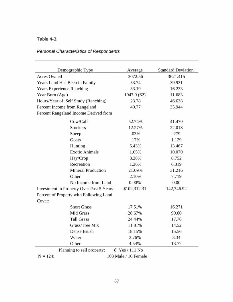
87
Table 4-3.
Personal Characteristics of Respondents
Demographic Type
Average
Standard Deviation
Acres Owned 3072.56 3621.415
Years Land Has Been in Family 53.74 39.931
Years Experience Ranching 33.19 16.233
Year Born (Age) 1947.9 (62) 11.683
Hours/Year of Self Study (Ranching) 23.78 46.638
Percent Income from Rangeland 40.77 35.944
Percent Rangeland Income Derived from
Cow/Calf 52.74% 41.470
Stockers 12.27% 22.018
Sheep .03% .279
Goats .17% 1.129
Hunting 5.43% 13.467
Exotic Animals 1.65% 10.070
Hay/Crop 3.28% 8.752
Recreation 1.26% 6.319
Mineral Production 21.09% 31.216
Other 2.10% 7.719
No Income from Land 0.00% 0.00
Investment in Property Over Past 5 Years $102,312.31 142,746.92
Percent of Property with Following Land
Cover:
Short Grass 17.51% 16.271
Mid Grass 28.67% 90.60
Tall Grass 24.44% 17.76
Grass/Tree Mix 11.81% 14.52
Dense Brush 18.15% 15.56
Water 3.76% 3.34
Other 4.54% 13.72
Planning to sell property: 8 Yes / 111 No
N = 124: 103 Male / 16 Female
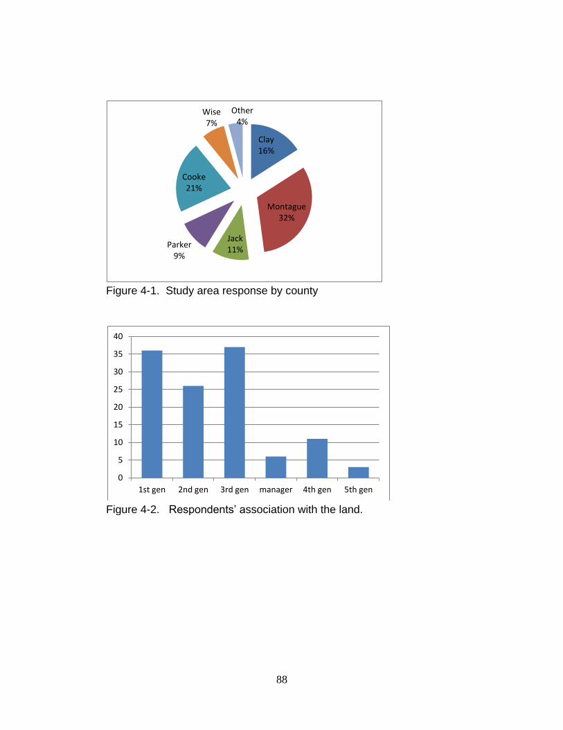
88
Figure 4-1. Study area response by county
Figure 4-2. Respondents’ association with the land.
Clay 16%
Montague 32%
Jack 11%
Parker 9%
Cooke 21%
Wise 7%
Other 4%
0
5
10
15
20
25
30
35
40
1st gen 2nd gen 3rd gen manager 4th gen 5th gen
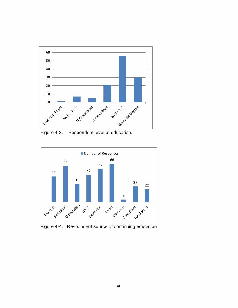
89
Figure 4-3. Respondent level of education.
Figure 4-4. Respondent source of continuing education
44
62
31
47
57
66
4
27 22
Number of Responses
0
10
20
30
40
50
60
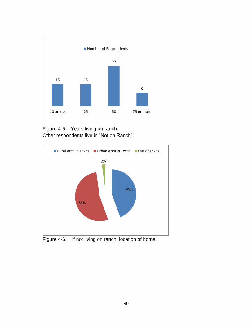
90
Figure 4-5. Years living on ranch.
Other respondents live in “Not on Ranch”.
Figure 4-6. If not living on ranch, location of home.
15 15
27
9
10 or less 25 50 75 or more
Number of Respondents
45%
53%
2%
Rural Area in Texas Urban Area in Texas Out of Texas
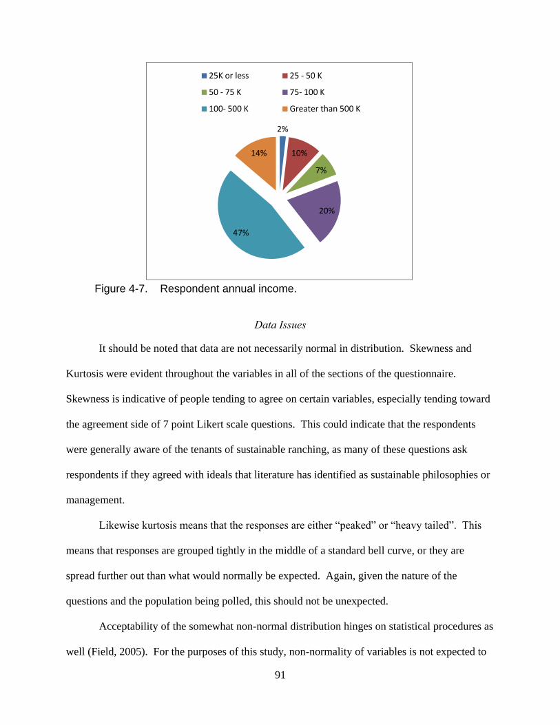
91
Data Issues
It should be noted that data are not necessarily normal in distribution. Skewness and
Kurtosis were evident throughout the variables in all of the sections of the questionnaire.
Skewness is indicative of people tending to agree on certain variables, especially tending toward
the agreement side of 7 point Likert scale questions. This could indicate that the respondents
were generally aware of the tenants of sustainable ranching, as many of these questions ask
respondents if they agreed with ideals that literature has identified as sustainable philosophies or
management.
Likewise kurtosis means that the responses are either ―peaked‖ or ―heavy tailed‖. This
means that responses are grouped tightly in the middle of a standard bell curve, or they are
spread further out than what would normally be expected. Again, given the nature of the
questions and the population being polled, this should not be unexpected.
Acceptability of the somewhat non-normal distribution hinges on statistical procedures as
well (Field, 2005). For the purposes of this study, non-normality of variables is not expected to
Figure 4-7. Respondent annual income.
2%
10%
7%
20%
47%
14%
25K or less 25 - 50 K
50 - 75 K 75- 100 K
100- 500 K Greater than 500 K
92
present a problem. Regression models make no distributional assumptions about the
independent variables themselves. However, residual error must be normally distributed for
smaller samples sizes. Where error is not normally distributed, t-tests of regression coefficients
are not accurate. (Garson, 2011b) and PCA only requires normality for certain significance test;
when performing PCA merely to gain factor scores, ―significance testing is beside the point‖
(Garson, 2011d).
Statistical Procedures
The ultimate goal of the data analysis was to analyze the set of variables to determine
relationship to sustainability. Statistical procedures are carried out in nine steps. Seven steps are
in preparation for multiple regression analysis. One step is the regression and the last step is
checking for non-response bias.
Removal of Missing Data
The number of respondents multiplied by the number of variables (124 x 218) made it
possible to have values in 27,032 cells. The raw data contained 1211 missing values in those
cells. Of those 1108 were simply not filled in, 103 were coded as don‘t know (DK) by the
respondent.
Independent samples t-test was used to check for significant differences in characteristics
between those respondents with missing data, and those without to test if data are Missing
Completely at Random (MCAR). It was found that there was a significant difference (p = < .01)
in percent income derived from the ranch land between the groups. Levene's Test for Equality of
Variances confirmed equality of variance between the groups (F = 6.346; p = .017. This
indicates the ―missingness‖ is not MCAR, therefore data imputation is appropriate. Application
of software available in the R environment, package ‗seqKNN‘, replaced all missing data.
93
Internal Consistency
Economic Sustainability
The initial computation for Cronbach‘s alpha coefficient, using all 14 variables in section
2, ―Economic Considerations‖, did not meet minimum critical value (α = .484). SPSS computed
"Cronbach's Alpha if Item Deleted". This was the estimated value of alpha if the variable were
removed from the model. If "alpha if deleted" was lower for all items than for the computed
overall alpha, then no further removal of variables was necessary. Variables were systematically
removed using this procedure, until Cronbach‘s alpha was maximized by retaining 6 variables (α
= .722). This exceeds the critical value (α = .70).
The six variables which maximize Cronbach‘s Alpha for ―Economic Considerations‖ are
identified as:
1. Financial risk can be reduced by implementation of proper grazing practices.
2. Proper grazing management of rangeland will positively influence the long-term
profitability of a ranch.
3. Deterioration of range conditions will cause log-term economic difficulties.
4. When compared to other ranches, I perceive the rate of return that I receive from grazing
rangeland as being above average.
5. I consciously plan for long-term economic sustainability (5 or more years).
6. I know my production costs.
Land Health Sustainability
The initial computation for Cronbach‘s alpha coefficient, using all 25 variables from
section 4, ―Land Health‖, did not meet minimum critical value (α = .649). Variables were
systematically removed until Cronbach‘s alpha was maximized by retaining 18 variables (α =
.730). This exceeds the critical value (α = .70).
The 18 variables were all were related to self-assessments of change in land
characteristics. Respondents were instructed, ―Change in the environment is certain‖. They
were then asked, ―In relation to your property, please indicate your perception of the change
94
noticed for each issue over the past 10 years. The items may have increased, remained constant,
decreased, or unknown.
The validity of each variable identified when maximizing Cronbach‘s Alpha was
assessed. Two variables indicating a change in the population of quail and a change in the
population of wild hogs were removed from the index. This is because of the extreme
widespread reduction of quail and the rampant invasion of wild hogs noticed across the state. It
was hypothesized that these two variables were indicators of a phenomena that exists regardless
of philosophy, management or personal characteristics. Selection of only the 16 remaining
variables maintained an Alpha coefficient of α = .71, which is still above the critical value.
‖ The 16 variables which used in the Land Health Sustainability Index were:
Mesquite
Juniper
Other Brush
Bare Ground
Invasive Weed Species (thistle, cacti, greenbriar, etc.)
Livestock Trails
Gullies
Soil Compaction
Small Pedestals (rocks or plants that appear elevated)
Evidence of plant litter around obstructions like grass clumps and stones.
Other evidence of non-gully water flow patterns
Tall grasses
Short grasses
Turkey
Other birds
Deer
Social Sustainability
The initial computation for Cronbach‘s alpha coefficient, using all 33 variables in section
2, ―Economic Considerations‖, did not meet minimum critical value (α = .224). Variables were
95
systematically removed until Cronbach‘s alpha was maximized by retaining 6 variables (α =
.656). This did not exceed the critical value (α = .70).
With the variables used in section 5, ―Quality of Life‖, the critical value for Cronbach‘s
Alpha was not met, because the highest alpha achievable was 0.656, which is less than the
critical value of 0.70 (Nunnaly and Bernstein, 1994; Starkweather, 2011b).
Other sources have indicated instances exist where a ―moderate‖ value for Cronbach‘s
alpha (α = .6) can be accepted as meeting the critical value necessary for creation of a
meaningful scale, instead of strictly adhering to a more stringent value (α = .7 or α = .8)
(Karahoca et al., 2010; Winter et al., 2004; Leontitits and Pagge, 2007). Specifically, Winter et
al. (2004) accepted as relevant the moderate Cronbach alpha coefficient (α = .670) and Leontitis
and Pagge (2007) even proved that lower levels were highly significant and resulting scales
could be accepted. Therefore, the maximum Cronbach‘s alpha coefficient possible (α = .655)
was considered to meet critical levels necessary for creation of a scale.
This may seem arbitrary, given the prior standard of acceptance for Cronbach‘s alpha of
α = .7. The reason for the change was to prevent possible loss of information. In the context of
this dissertation, it is desirable to investigate the index further in order to fully understand all
methods and possible associations between variables and indices.
To increase the similarity of the derived quality of life, or social sustainability index to
relevant literature (West and Herrick, 2003), the variable indicating personal satisfaction of the
manager was re-introduced, because it was deemed useful in the derived quality of life index and
it affected the Cronbach‘s alpha minimally (α = .655). Seven variables from section 5 suggested
respondent‘s perceptions of key factors in relation to their quality of life. They are explained by
statements from the questionnaire as follows:
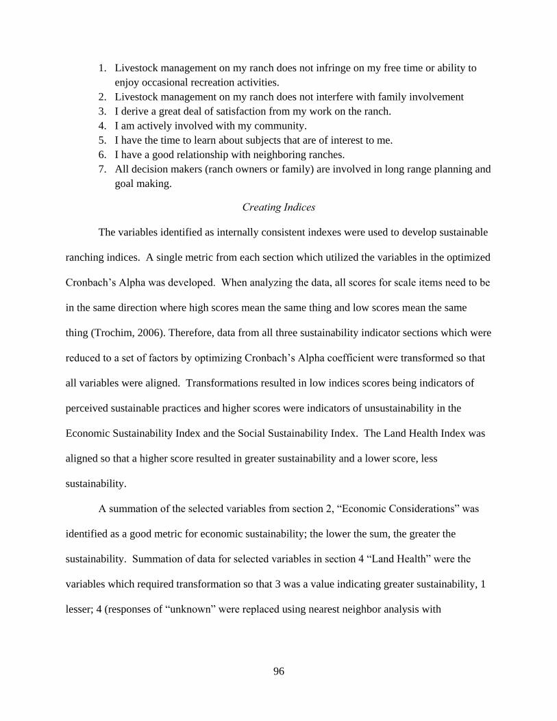
96
1. Livestock management on my ranch does not infringe on my free time or ability to
enjoy occasional recreation activities.
2. Livestock management on my ranch does not interfere with family involvement
3. I derive a great deal of satisfaction from my work on the ranch.
4. I am actively involved with my community.
5. I have the time to learn about subjects that are of interest to me.
6. I have a good relationship with neighboring ranches.
7. All decision makers (ranch owners or family) are involved in long range planning and
goal making.
Creating Indices
The variables identified as internally consistent indexes were used to develop sustainable
ranching indices. A single metric from each section which utilized the variables in the optimized
Cronbach‘s Alpha was developed. When analyzing the data, all scores for scale items need to be
in the same direction where high scores mean the same thing and low scores mean the same
thing (Trochim, 2006). Therefore, data from all three sustainability indicator sections which were
reduced to a set of factors by optimizing Cronbach‘s Alpha coefficient were transformed so that
all variables were aligned. Transformations resulted in low indices scores being indicators of
perceived sustainable practices and higher scores were indicators of unsustainability in the
Economic Sustainability Index and the Social Sustainability Index. The Land Health Index was
aligned so that a higher score resulted in greater sustainability and a lower score, less
sustainability.
A summation of the selected variables from section 2, ―Economic Considerations‖ was
identified as a good metric for economic sustainability; the lower the sum, the greater the
sustainability. Summation of data for selected variables in section 4 ―Land Health‖ were the
variables which required transformation so that 3 was a value indicating greater sustainability, 1
lesser; 4 (responses of ―unknown‖ were replaced using nearest neighbor analysis with
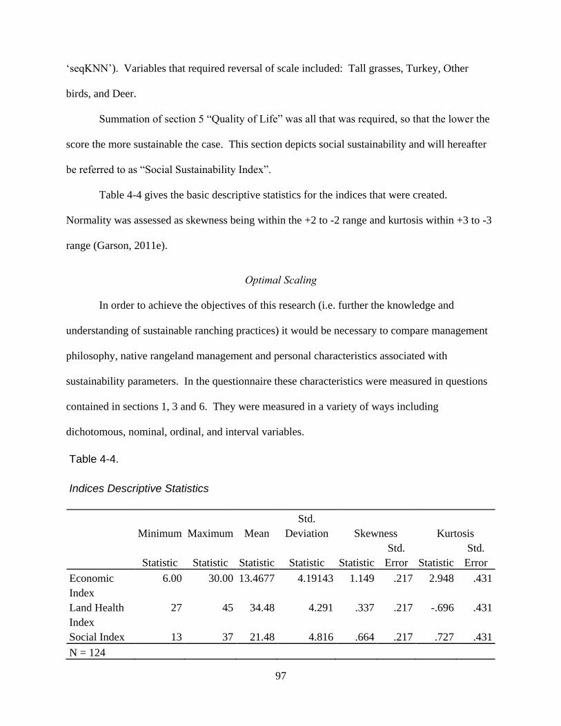
97
‗seqKNN‘). Variables that required reversal of scale included: Tall grasses, Turkey, Other
birds, and Deer.
Summation of section 5 ―Quality of Life‖ was all that was required, so that the lower the
score the more sustainable the case. This section depicts social sustainability and will hereafter
be referred to as ―Social Sustainability Index‖.
Table 4-4 gives the basic descriptive statistics for the indices that were created.
Normality was assessed as skewness being within the +2 to -2 range and kurtosis within +3 to -3
range (Garson, 2011e).
Optimal Scaling
In order to achieve the objectives of this research (i.e. further the knowledge and
understanding of sustainable ranching practices) it would be necessary to compare management
philosophy, native rangeland management and personal characteristics associated with
sustainability parameters. In the questionnaire these characteristics were measured in questions
contained in sections 1, 3 and 6. They were measured in a variety of ways including
dichotomous, nominal, ordinal, and interval variables.
Table 4-4.
Indices Descriptive Statistics
Minimum Maximum Mean
Std.
Deviation Skewness Kurtosis
Statistic Statistic Statistic Statistic Statistic
Std.
Error Statistic
Std.
Error
Economic
Index
6.00 30.00 13.4677 4.19143 1.149 .217 2.948 .431
Land Health
Index
27 45 34.48 4.291 .337 .217 -.696 .431
Social Index 13 37 21.48 4.816 .664 .217 .727 .431
N = 124
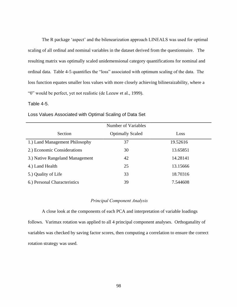
98
The R package ‗aspect‘ and the bilenearization approach LINEALS was used for optimal
scaling of all ordinal and nominal variables in the dataset derived from the questionnaire. The
resulting matrix was optimally scaled unidemensional category quantifications for nominal and
ordinal data. Table 4-5 quantifies the ―loss‖ associated with optimum scaling of the data. The
loss function equates smaller loss values with more closely achieving bilineraizability, where a
―0‖ would be perfect, yet not realistic (de Leeuw et al., 1999).
Table 4-5.
Loss Values Associated with Optimal Scaling of Data Set
Section
Number of Variables
Optimally Scaled Loss
1.) Land Management Philosophy 37 19.52616
2.) Economic Considerations 30 13.65851
3.) Native Rangeland Management 42 14.28141
4.) Land Health 25 13.15666
5.) Quality of Life 33 18.70316
6.) Personal Characteristics 39 7.544608
Principal Component Analysis
A close look at the components of each PCA and interpretation of variable loadings
follows. Varimax rotation was applied to all 4 principal component analyses. Orthoganality of
variables was checked by saving factor scores, then computing a correlation to ensure the correct
rotation strategy was used.
99
PCA 1: Land Management Philosophy (4 components)
Section 1, Land Management Philosophy, contained 37 separate variables. The parallel
engine analysis (Patil, 2008) eigenvalues for random data coincided with eigenvalues from
section 1, when 3 components were accepted, percentile values of 2.018843 and 2.457
respectively, then dropping to eigenvalues of 1.814744 and 1.786 on the 4th
component. The
scree plot on the other hand identified either 4 or 5 components (Figure 4-8). A compromise
seemed logical and 4 components were selected which explained 40.131% of the variance in the
unrotated model. Varimax rotation was applied, the variance explained remained at 40.131%.
Figure 4-8. Scree Plot Principal Component Analysis 1.
The KMO statistic is well within the specified range for sample adequacy (0.74). The
Bartlett‘s Test of Sphericity is highly significant (p < .001) that the correlation matrix is not an
identity matrix (Table 4-6); indicating variables in the population correlation matrix are
uncorrelated. Therefore it may be assumed multicollinearity is not a problem. The observed
significance level here allows rejection of the null hypothesis. It is concluded that the strength of
the relationship among variables is strong, but not multicollinear.
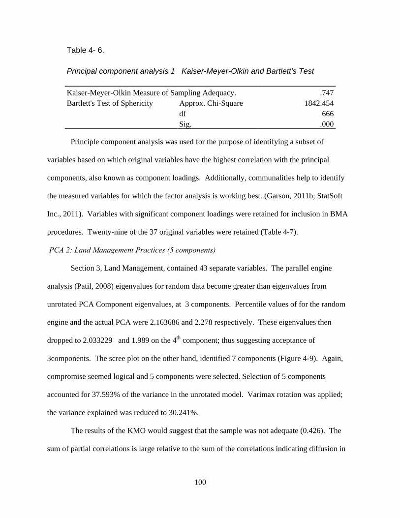
100
Principle component analysis was used for the purpose of identifying a subset of
variables based on which original variables have the highest correlation with the principal
components, also known as component loadings. Additionally, communalities help to identify
the measured variables for which the factor analysis is working best. (Garson, 2011b; StatSoft
Inc., 2011). Variables with significant component loadings were retained for inclusion in BMA
procedures. Twenty-nine of the 37 original variables were retained (Table 4-7).
PCA 2: Land Management Practices (5 components)
Section 3, Land Management, contained 43 separate variables. The parallel engine
analysis (Patil, 2008) eigenvalues for random data become greater than eigenvalues from
unrotated PCA Component eigenvalues, at 3 components. Percentile values of for the random
engine and the actual PCA were 2.163686 and 2.278 respectively. These eigenvalues then
dropped to 2.033229 and 1.989 on the 4th
component; thus suggesting acceptance of
3components. The scree plot on the other hand, identified 7 components (Figure 4-9). Again,
compromise seemed logical and 5 components were selected. Selection of 5 components
accounted for 37.593% of the variance in the unrotated model. Varimax rotation was applied;
the variance explained was reduced to 30.241%.
The results of the KMO would suggest that the sample was not adequate (0.426). The
sum of partial correlations is large relative to the sum of the correlations indicating diffusion in
Table 4- 6.
Principal component analysis 1 Kaiser-Meyer-Olkin and Bartlett's Test
Kaiser-Meyer-Olkin Measure of Sampling Adequacy. .747
Bartlett's Test of Sphericity Approx. Chi-Square 1842.454
df 666
Sig. .000
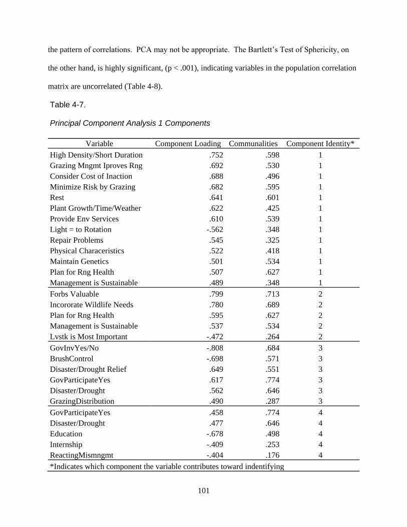
101
the pattern of correlations. PCA may not be appropriate. The Bartlett‘s Test of Sphericity, on
the other hand, is highly significant, (p < .001), indicating variables in the population correlation
matrix are uncorrelated (Table 4-8).
Table 4-7. Principal Component Analysis 1 Components
Variable Component Loading Communalities Component Identity*
High Density/Short Duration .752 .598 1
Grazing Mngmt Iproves Rng .692 .530 1
Consider Cost of Inaction .688 .496 1
Minimize Risk by Grazing .682 .595 1
Rest .641 .601 1
Plant Growth/Time/Weather .622 .425 1
Provide Env Services .610 .539 1
Light = to Rotation -.562 .348 1
Repair Problems .545 .325 1
Physical Characeristics .522 .418 1
Maintain Genetics .501 .534 1
Plan for Rng Health .507 .627 1
Management is Sustainable .489 .348 1
Forbs Valuable .799 .713 2
Incororate Wildlife Needs .780 .689 2
Plan for Rng Health .595 .627 2
Management is Sustainable .537 .534 2
Lvstk is Most Important -.472 .264 2
GovInvYes/No -.808 .684 3
BrushControl -.698 .571 3
Disaster/Drought Relief .649 .551 3
GovParticipateYes .617 .774 3
Disaster/Drought .562 .646 3
GrazingDistribution .490 .287 3
GovParticipateYes .458 .774 4
Disaster/Drought .477 .646 4
Education -.678 .498 4
Internship -.409 .253 4
ReactingMismngmt -.404 .176 4
*Indicates which component the variable contributes toward indentifying
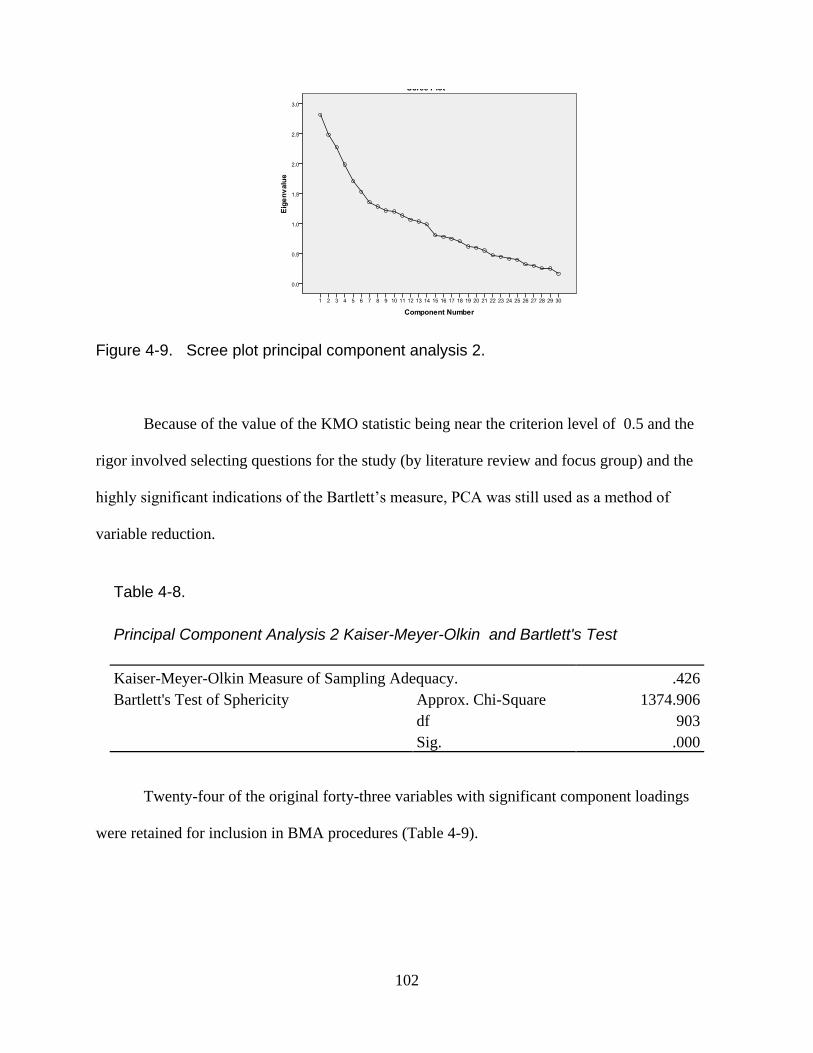
102
Figure 4-9. Scree plot principal component analysis 2.
Because of the value of the KMO statistic being near the criterion level of 0.5 and the
rigor involved selecting questions for the study (by literature review and focus group) and the
highly significant indications of the Bartlett‘s measure, PCA was still used as a method of
variable reduction.
Table 4-8.
Principal Component Analysis 2 Kaiser-Meyer-Olkin and Bartlett's Test
Kaiser-Meyer-Olkin Measure of Sampling Adequacy. .426
Bartlett's Test of Sphericity Approx. Chi-Square 1374.906
df 903
Sig. .000
Twenty-four of the original forty-three variables with significant component loadings
were retained for inclusion in BMA procedures (Table 4-9).
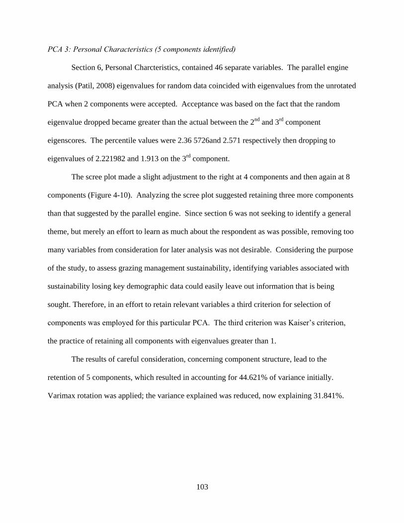
103
PCA 3: Personal Characteristics (5 components identified)
Section 6, Personal Charcteristics, contained 46 separate variables. The parallel engine
analysis (Patil, 2008) eigenvalues for random data coincided with eigenvalues from the unrotated
PCA when 2 components were accepted. Acceptance was based on the fact that the random
eigenvalue dropped became greater than the actual between the 2nd
and 3rd
component
eigenscores. The percentile values were 2.36 5726and 2.571 respectively then dropping to
eigenvalues of 2.221982 and 1.913 on the 3rd
component.
The scree plot made a slight adjustment to the right at 4 components and then again at 8
components (Figure 4-10). Analyzing the scree plot suggested retaining three more components
than that suggested by the parallel engine. Since section 6 was not seeking to identify a general
theme, but merely an effort to learn as much about the respondent as was possible, removing too
many variables from consideration for later analysis was not desirable. Considering the purpose
of the study, to assess grazing management sustainability, identifying variables associated with
sustainability losing key demographic data could easily leave out information that is being
sought. Therefore, in an effort to retain relevant variables a third criterion for selection of
components was employed for this particular PCA. The third criterion was Kaiser‘s criterion,
the practice of retaining all components with eigenvalues greater than 1.
The results of careful consideration, concerning component structure, lead to the
retention of 5 components, which resulted in accounting for 44.621% of variance initially.
Varimax rotation was applied; the variance explained was reduced, now explaining 31.841%.
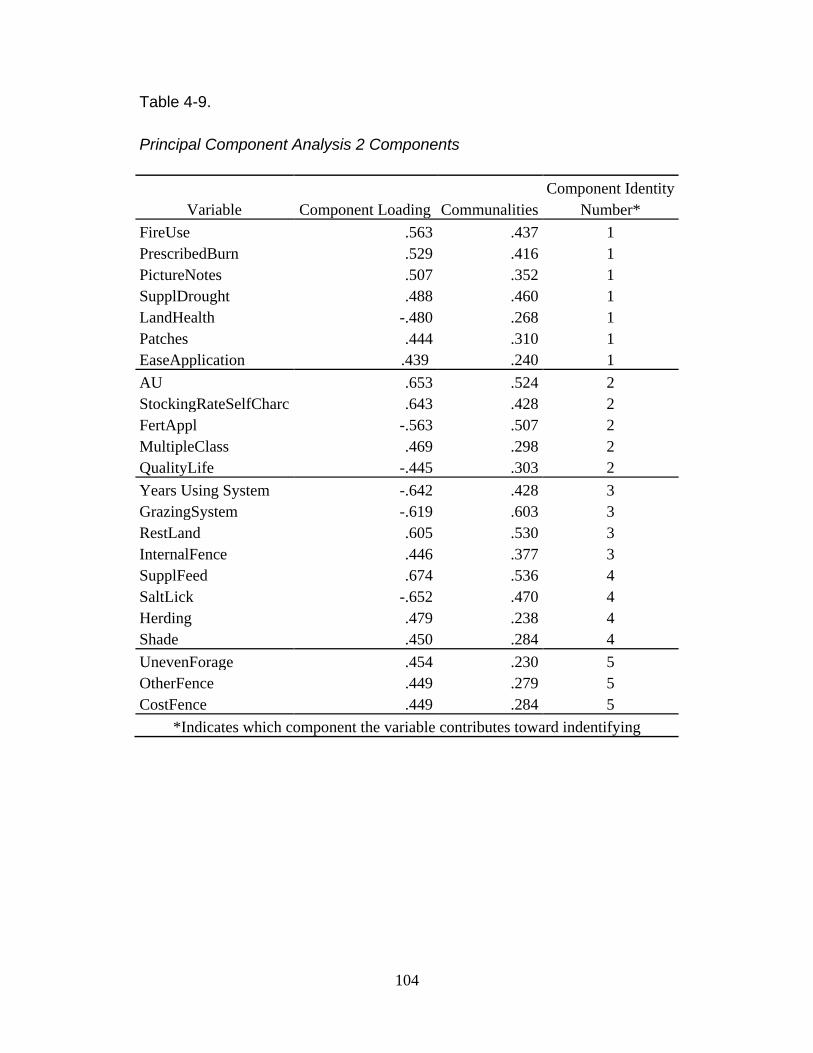
104
Table 4-9.
Principal Component Analysis 2 Components
Variable Component Loading Communalities
Component Identity
Number*
FireUse .563 .437 1
PrescribedBurn .529 .416 1
PictureNotes .507 .352 1
SupplDrought .488 .460 1
LandHealth -.480 .268 1
Patches .444 .310 1
EaseApplication .439 .240 1
AU .653 .524 2
StockingRateSelfCharc .643 .428 2
FertAppl -.563 .507 2
MultipleClass .469 .298 2
QualityLife -.445 .303 2
Years Using System -.642 .428 3
GrazingSystem -.619 .603 3
RestLand .605 .530 3
InternalFence .446 .377 3
SupplFeed .674 .536 4
SaltLick -.652 .470 4
Herding .479 .238 4
Shade .450 .284 4
UnevenForage .454 .230 5
OtherFence .449 .279 5
CostFence .449 .284 5
*Indicates which component the variable contributes toward indentifying
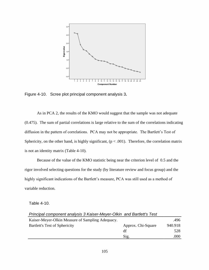
105
Figure 4-10. Scree plot principal component analysis 3.
As in PCA 2, the results of the KMO would suggest that the sample was not adequate
(0.475). The sum of partial correlations is large relative to the sum of the correlations indicating
diffusion in the pattern of correlations. PCA may not be appropriate. The Bartlett‘s Test of
Sphericity, on the other hand, is highly significant, (p < .001). Therefore, the correlation matrix
is not an identity matrix (Table 4-10).
Because of the value of the KMO statistic being near the criterion level of 0.5 and the
rigor involved selecting questions for the study (by literature review and focus group) and the
highly significant indications of the Bartlett‘s measure, PCA was still used as a method of
variable reduction.
Table 4-10.
Principal component analysis 3 Kaiser-Meyer-Olkin and Bartlett's Test
Kaiser-Meyer-Olkin Measure of Sampling Adequacy. .496
Bartlett's Test of Sphericity Approx. Chi-Square 940.918
df 528
Sig. .000
106
Twenty-six of the original forty-six variables with significant component loadings were
retained for inclusion in BMA procedures (Table 4-11).
PCA 4: Other Variables (8 components identified)
The PCA which was run on ―Other variables‖ was use as a means of retaining variables
that were left behind from section 2, 4, and 5 during the creation of scales to create indices.
This resulted in the inclusion of 55 separate variables. The parallel engine analysis (Patil, 2008)
identified 7components as important. Comparison of eigenvalues between the random data and
the actual data between the 7th
and the 8th
component were 1.998811 and 2.041 then dropping to
eigenvalues of 1.926439 and 1.821 respectively.
The scree plot developed a crook at 7 components, but clearly trailed to the right at 8
components (Figure 4-11). Also, there were 21 components with eigenvalues greater than 1.
Therefore, 8 components were selected to retain in the analysis. The initial variance explained
by the 8 components was 39.341%; after varimax rotation the variance explained remained at
39.341%.
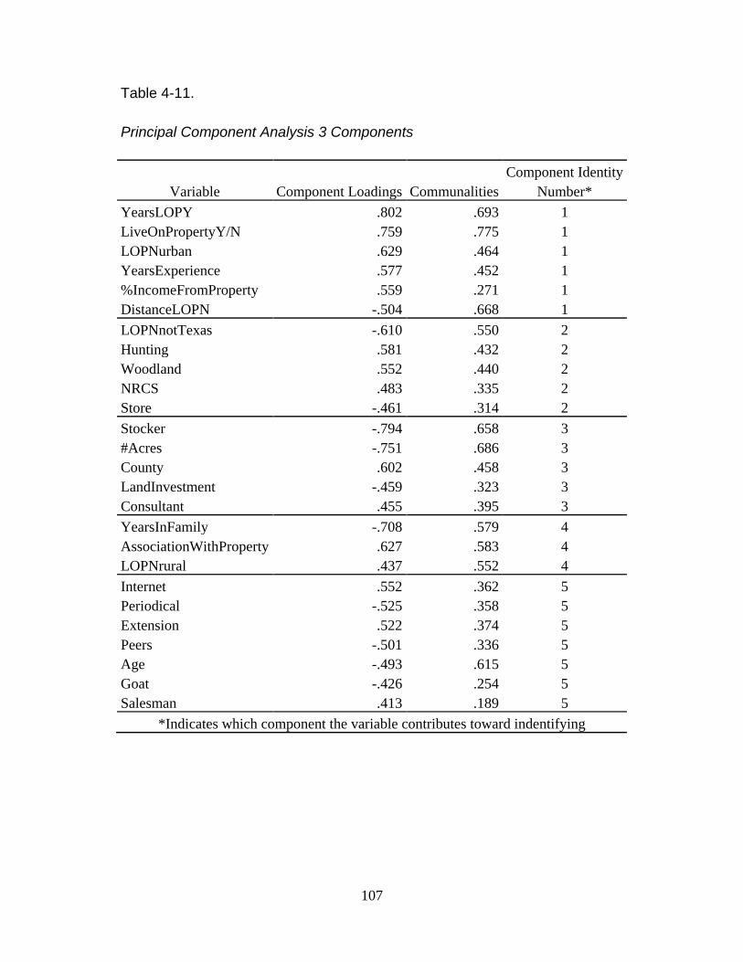
107
Table 4-11.
Principal Component Analysis 3 Components
Variable Component Loadings Communalities
Component Identity
Number*
YearsLOPY .802 .693 1
LiveOnPropertyY/N .759 .775 1
LOPNurban .629 .464 1
YearsExperience .577 .452 1
%IncomeFromProperty .559 .271 1
DistanceLOPN -.504 .668 1
LOPNnotTexas -.610 .550 2
Hunting .581 .432 2
Woodland .552 .440 2
NRCS .483 .335 2
Store -.461 .314 2
Stocker -.794 .658 3
#Acres -.751 .686 3
County .602 .458 3
LandInvestment -.459 .323 3
Consultant .455 .395 3
YearsInFamily -.708 .579 4
AssociationWithProperty .627 .583 4
LOPNrural .437 .552 4
Internet .552 .362 5
Periodical -.525 .358 5
Extension .522 .374 5
Peers -.501 .336 5
Age -.493 .615 5
Goat -.426 .254 5
Salesman .413 .189 5
*Indicates which component the variable contributes toward indentifying
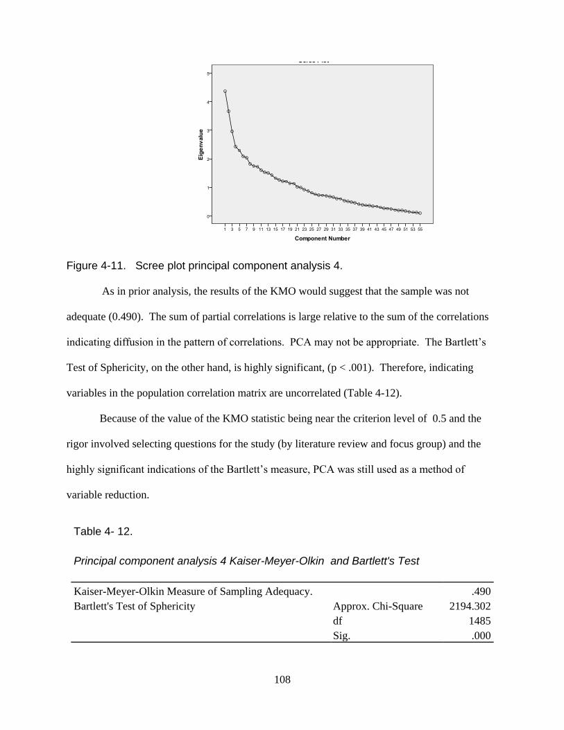
108
Figure 4-11. Scree plot principal component analysis 4.
As in prior analysis, the results of the KMO would suggest that the sample was not
adequate (0.490). The sum of partial correlations is large relative to the sum of the correlations
indicating diffusion in the pattern of correlations. PCA may not be appropriate. The Bartlett‘s
Test of Sphericity, on the other hand, is highly significant, (p < .001). Therefore, indicating
variables in the population correlation matrix are uncorrelated (Table 4-12).
Because of the value of the KMO statistic being near the criterion level of 0.5 and the
rigor involved selecting questions for the study (by literature review and focus group) and the
highly significant indications of the Bartlett‘s measure, PCA was still used as a method of
variable reduction.
Table 4- 12.
Principal component analysis 4 Kaiser-Meyer-Olkin and Bartlett's Test
Kaiser-Meyer-Olkin Measure of Sampling Adequacy. .490
Bartlett's Test of Sphericity Approx. Chi-Square 2194.302
df 1485
Sig. .000
109
Thirty-seven of the original fifty-five variables with significant component loadings were
retained for inclusion in BMA procedures (Table 4-13).
In all the results of 4 principal component analyses have reduced the total number of
variables from 193 to 110. The total variables could have been reduced to a greater extent if a
more stringent parameter had been employed for deletion of variables.
The PCA was conducted primarily to help reduce the number of variables for
consideration using regression analysis. An alternative to using the PCA would have been
arbitrarily choosing variables based on the literature review and on the focus group session. The
greatest threat to the PCA successfully reducing the number of variables was the fact that the
KMO statistic is based on correlation and partial correlation. KMO did not indicate that data
were likely to load on factors well. In the past the conclusion was that a factor analysis should
be run. This was extremely useful before computers, allowing researchers to save much
unnecessary work. Now, with the relative ease of computing multiple PCA or factor analyses
quickly, KMO is more useful for assessing issues with multicollinearity (Garson 2011b).
KMO values range between 0 and 1. A value closer to 1 indicates that patterns of
correlations are relatively compact and so far as factor analysis should yield distinct and reliable
factors; whereas values above .5 are acceptable. ―Values below that should cause one to rethink
which variables to include‖ (Field, 2005). Garson (2011b) also indicates that variables may be
removed prior to factor analysis based on low individual KMO scores, which will make PCA or
factor analysis more amiable. Considering this study chose to retain variables with high
component loadings, which are the correlation coefficients between the variables and the
components, it is unlikely that these would be variables removed in order to increase KMO.
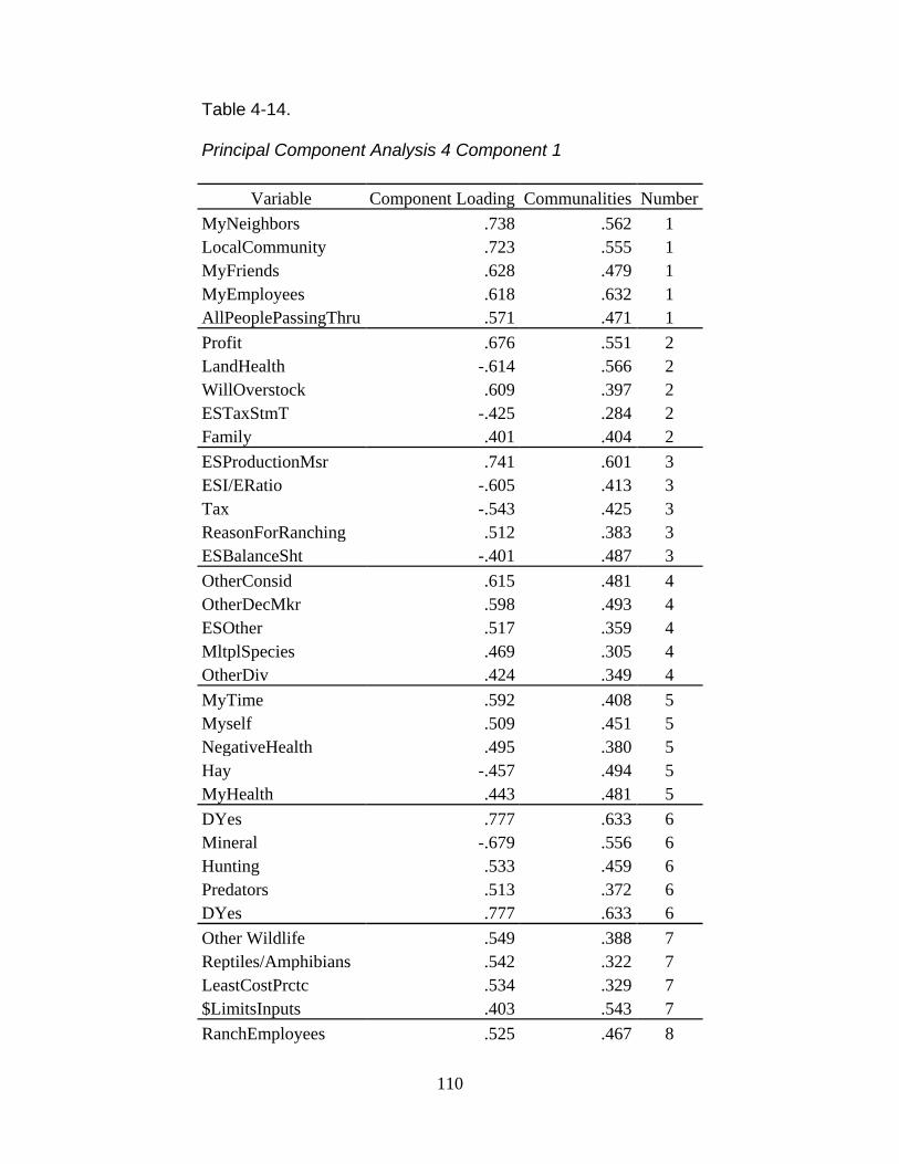
110
Table 4-14. Principal Component Analysis 4 Component 1
Variable Component Loading Communalities Number
MyNeighbors .738 .562 1
LocalCommunity .723 .555 1
MyFriends .628 .479 1
MyEmployees .618 .632 1
AllPeoplePassingThru .571 .471 1
Profit .676 .551 2
LandHealth -.614 .566 2
WillOverstock .609 .397 2
ESTaxStmT -.425 .284 2
Family .401 .404 2
ESProductionMsr .741 .601 3
ESI/ERatio -.605 .413 3
Tax -.543 .425 3
ReasonForRanching .512 .383 3
ESBalanceSht -.401 .487 3
OtherConsid .615 .481 4
OtherDecMkr .598 .493 4
ESOther .517 .359 4
MltplSpecies .469 .305 4
OtherDiv .424 .349 4
MyTime .592 .408 5
Myself .509 .451 5
NegativeHealth .495 .380 5
Hay -.457 .494 5
MyHealth .443 .481 5
DYes .777 .633 6
Mineral -.679 .556 6
Hunting .533 .459 6
Predators .513 .372 6
DYes .777 .633 6
Other Wildlife .549 .388 7
Reptiles/Amphibians .542 .322 7
LeastCostPrctc .534 .329 7
$LimitsInputs .403 .543 7
RanchEmployees .525 .467 8
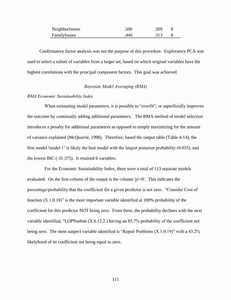
111
NeighborIssues .500 .309 8
FamilyIssues .446 .313 8
Confirmatory factor analysis was not the purpose of this procedure. Exploratory PCA was
used to select a subset of variables from a larger set, based on which original variables have the
highest correlations with the principal component factors. This goal was achieved.
Bayesian Model Averaging (BMA)
BMA Economic Sustainability Index
When estimating model parameters, it is possible to ―overfit‖; or superficially improves
the outcome by continually adding additional parameters. The BMA method of model selection
introduces a penalty for additional parameters as opposed to simply maximizing for the amount
of variance explained (McQuarrie, 1998). Therefore, based the output table (Table 4-14), the
first model 'model 1‘ is likely the best model with the largest posterior probability (0.035), and
the lowest BIC (-31.375). It retained 6 variables.
For the Economic Sustainability Index, there were a total of 113 separate models
evaluated. On the first column of the output is the column 'p!=0'. This indicates the
percentage/probability that the coefficient for a given predictor is not zero. ―Consider Cost of
Inaction (X.1.0.18)‖ is the most important variable identified at 100% probability of the
coefficient for this predictor NOT being zero. From there, the probability declines with the next
variable identified, ―LOPNurban (X.6.12.2.) having an 85.7% probability of the coefficient not
being zero. The most suspect variable identified is ―Repair Problems (X.1.0.19)‖ with a 43.2%
likelyhood of its coefficient not being equal to zero.
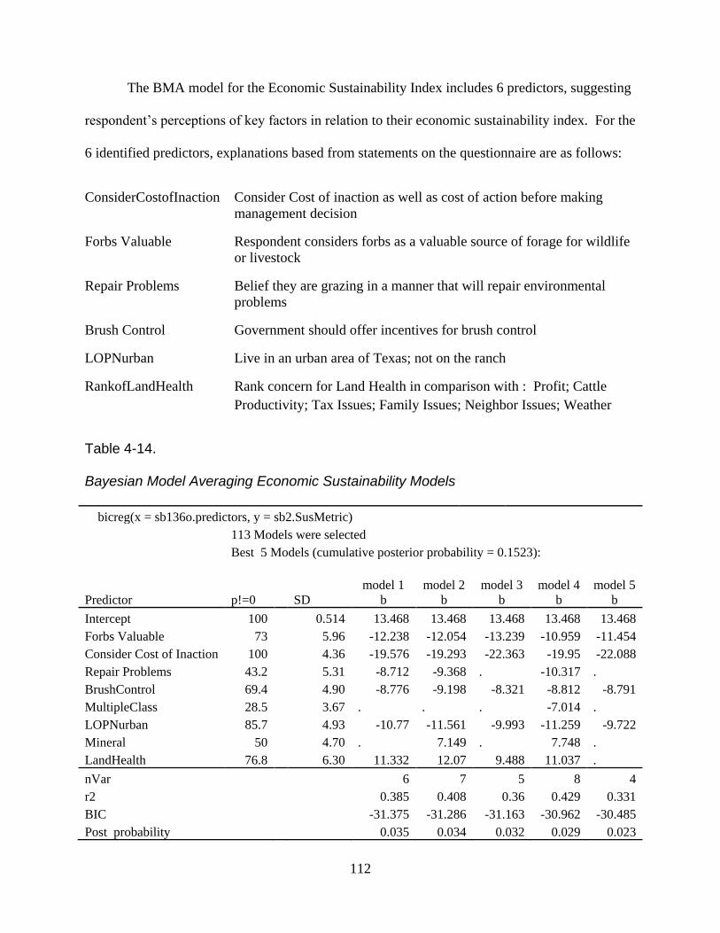
112
The BMA model for the Economic Sustainability Index includes 6 predictors, suggesting
respondent‘s perceptions of key factors in relation to their economic sustainability index. For the
6 identified predictors, explanations based from statements on the questionnaire are as follows:
ConsiderCostofInaction Consider Cost of inaction as well as cost of action before making
management decision
Forbs Valuable Respondent considers forbs as a valuable source of forage for wildlife
or livestock
Repair Problems Belief they are grazing in a manner that will repair environmental
problems
Brush Control Government should offer incentives for brush control
LOPNurban Live in an urban area of Texas; not on the ranch
RankofLandHealth Rank concern for Land Health in comparison with : Profit; Cattle
Productivity; Tax Issues; Family Issues; Neighbor Issues; Weather
Table 4-14. Bayesian Model Averaging Economic Sustainability Models
bicreg(x = sb136o.predictors, y = sb2.SusMetric)
113 Models were selected
Best 5 Models (cumulative posterior probability = 0.1523):
Predictor p!=0 SD
model 1
b
model 2
b
model 3
b
model 4
b
model 5
b
Intercept 100 0.514 13.468 13.468 13.468 13.468 13.468
Forbs Valuable 73 5.96 -12.238 -12.054 -13.239 -10.959 -11.454
Consider Cost of Inaction 100 4.36 -19.576 -19.293 -22.363 -19.95 -22.088
Repair Problems 43.2 5.31 -8.712 -9.368 . -10.317 .
BrushControl 69.4 4.90 -8.776 -9.198 -8.321 -8.812 -8.791
MultipleClass 28.5 3.67 . . . -7.014 .
LOPNurban 85.7 4.93 -10.77 -11.561 -9.993 -11.259 -9.722
Mineral 50 4.70 . 7.149 . 7.748 .
LandHealth 76.8 6.30 11.332 12.07 9.488 11.037 .
nVar 6 7 5 8 4
r2 0.385 0.408 0.36 0.429 0.331
BIC -31.375 -31.286 -31.163 -30.962 -30.485
Post probability 0.035 0.034 0.032 0.029 0.023
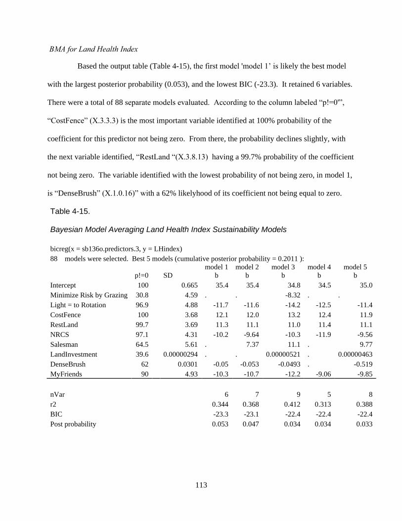
113
BMA for Land Health Index
Based the output table (Table 4-15), the first model 'model 1‘ is likely the best model
with the largest posterior probability (0.053), and the lowest BIC (-23.3). It retained 6 variables.
There were a total of 88 separate models evaluated. According to the column labeled ―p!=0'‖,
―CostFence‖ (X.3.3.3) is the most important variable identified at 100% probability of the
coefficient for this predictor not being zero. From there, the probability declines slightly, with
the next variable identified, ―RestLand ―(X.3.8.13) having a 99.7% probability of the coefficient
not being zero. The variable identified with the lowest probability of not being zero, in model 1,
is ―DenseBrush‖ (X.1.0.16)‖ with a 62% likelyhood of its coefficient not being equal to zero.
Table 4-15. Bayesian Model Averaging Land Health Index Sustainability Models
bicreg(x = sb136o.predictors.3, y = LHindex)
88 models were selected. Best 5 models (cumulative posterior probability = 0.2011 ):
p!=0
SD
model 1
b
model 2
b
model 3
b
model 4
b
model 5
b
Intercept 100
0.665 35.4 35.4 34.8 34.5 35.0
Minimize Risk by Grazing 30.8
4.59 . . -8.32 . .
Light = to Rotation 96.9
4.88 -11.7 -11.6 -14.2 -12.5 -11.4
CostFence 100
3.68 12.1 12.0 13.2 12.4 11.9
RestLand 99.7
3.69 11.3 11.1 11.0 11.4 11.1
NRCS 97.1
4.31 -10.2 -9.64 -10.3 -11.9 -9.56
Salesman 64.5
5.61 . 7.37 11.1 . 9.77
LandInvestment 39.6
0.00000294 . . 0.00000521 . 0.00000463
DenseBrush 62
0.0301 -0.05 -0.053 -0.0493 . -0.519
MyFriends 90
4.93 -10.3 -10.7 -12.2 -9.06 -9.85
nVar
6 7 9 5 8
r2
0.344 0.368 0.412 0.313 0.388
BIC
-23.3 -23.1 -22.4 -22.4 -22.4
Post probability
0.053 0.047 0.034 0.034 0.033
114
The 6 predictors, from model 1, suggest respondent‘s perceptions of key factors in
relation to their economic sustainability index. For the 6 identified predictors, explanations
based from statements on the questionnaire are as follows:
Light = to Rotation Degree which respondents believe lightly or moderately stocked,
continuous grazing has ecological benefits equal to rotation of
livestock to different pastures.
CostFence Fence cost is an obstacle to increasing grazing distribution
RestLand Respondents rest the land for a portion of the growing season as a
critical component of my grazing plan.
NRCS Respondent uses the NRCS as a source of grazing management
information
DenseBrush Percent of respondent‘s native grassland currently covered by dense
brush or woodlands
My Freinds Respondents consider their friends when making management
decisions.
BMA for Social Sustainability Index
Based the output table, the first model 'model 1' is likely the best model with the
largest posterior probability (0.228), and the lowest BIC (-3.0872). This model retained six
variables (Table 4-16).
There were a total of 117 separate models evaluated. According to the column labeled
―p!=0'‖, ―Salesman (X.6.10.7)‖ is the most important variable identified at 97.9% probability of
the coefficient for this predictor NOT being zero. From there, the probability declines with the
next variable identified, ―Patches (X.3.8.8)‖ having an 87.2% probability of the coefficient not
being zero. The most suspect variable identified is ―Herding (X.3.4.1)‖ with a 38.5% likelyhood
of its coefficient not being equal to zero.
The six predictors, identified as having the best model fit, suggest respondent‘s
perceptions of key factors in relation to their social sustainability index. For the six identified
predictors, explanations based from statements on the questionnaire are as follows:
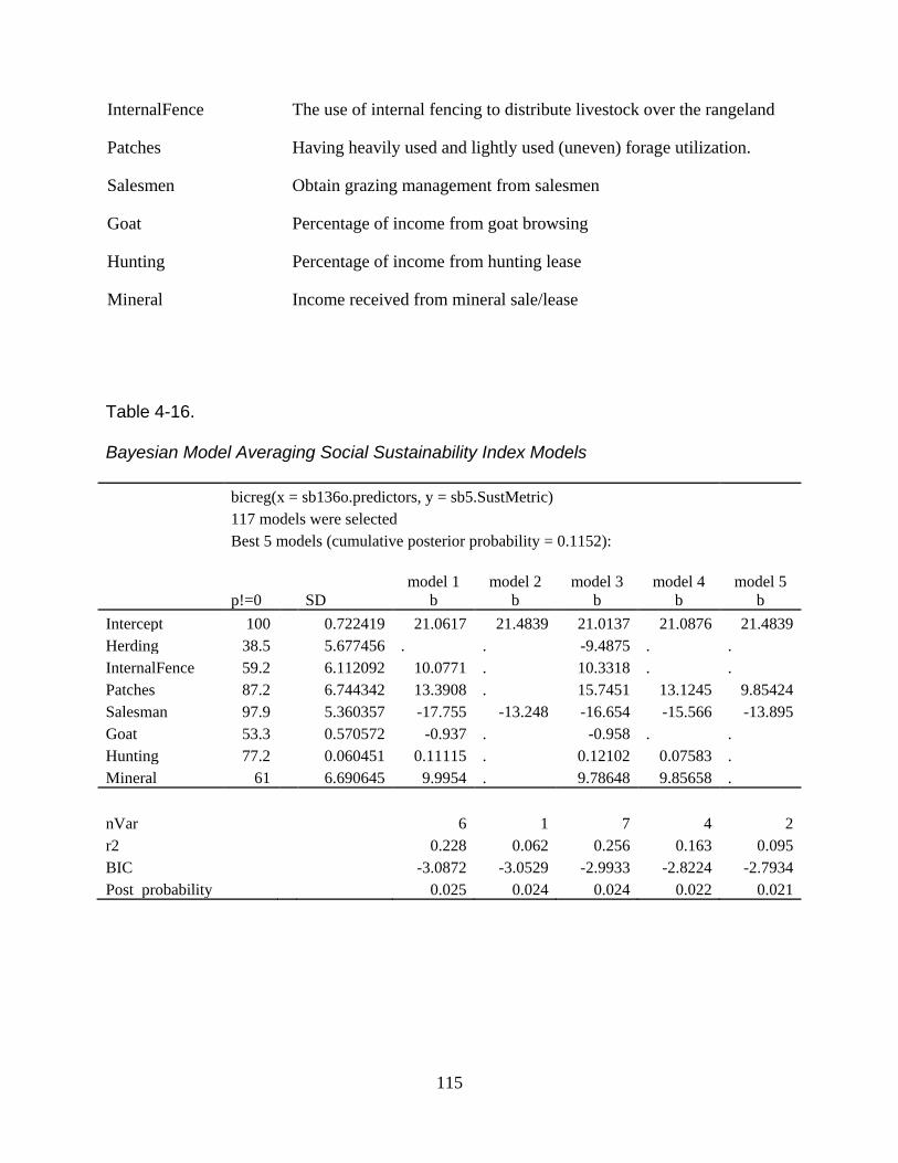
115
InternalFence The use of internal fencing to distribute livestock over the rangeland
Patches Having heavily used and lightly used (uneven) forage utilization.
Salesmen Obtain grazing management from salesmen
Goat Percentage of income from goat browsing
Hunting Percentage of income from hunting lease
Mineral Income received from mineral sale/lease
Table 4-16. Bayesian Model Averaging Social Sustainability Index Models
bicreg(x = sb136o.predictors, y = sb5.SustMetric)
117 models were selected
Best 5 models (cumulative posterior probability = 0.1152):
p!=0 SD
model 1
b
model 2
b
model 3
b
model 4
b
model 5
b
Intercept 100 0.722419 21.0617 21.4839 21.0137 21.0876 21.4839
Herding 38.5 5.677456 . . -9.4875 . .
InternalFence 59.2 6.112092 10.0771 . 10.3318 . .
Patches 87.2 6.744342 13.3908 . 15.7451 13.1245 9.85424
Salesman 97.9 5.360357 -17.755 -13.248 -16.654 -15.566 -13.895
Goat 53.3 0.570572 -0.937 . -0.958 . .
Hunting 77.2 0.060451 0.11115 . 0.12102 0.07583 .
Mineral 61 6.690645 9.9954 . 9.78648 9.85658 .
nVar 6 1 7 4 2
r2 0.228 0.062 0.256 0.163 0.095
BIC -3.0872 -3.0529 -2.9933 -2.8224 -2.7934
Post probability 0.025 0.024 0.024 0.022 0.021
116
Regression Analysis
Regression for Economic Sustainability Index
Economic sustainability index scores were regressed on land management philosophy
variables identified as the best model by Bayesian Model Averaging, using hierarchical
regression analysis (Table 4-17). The six predictors from BMA Economic Sustainability Index,
model 1, accounted for just under over 1/3 of the variance in economic sustainability index
scores in the final model (R2 = .385; adjusted R2
= .354; F(6,117) = 12.212; p < .001), which was
highly significant. Even though the best model only account for approximately 39% of the
variability in the respondents data, the model is considered significantly better than would be
expected by chance, and therefore the null hypothesis of no linear relationship of y to the
independents is rejected.
Model Validation
General assumptions for regression were met with block three from the original
model for Economic Sustainability Index. Cross-validation of the model was computed using R-
version 12.13.0 software, package ‗DAAG‘, which uses the K – fold method. In this procedure
K was selected as 4 to maintain a 5:1 ratio of cases to predictors for each fold. It was noted that
―Repair Problems‖ did not significantly contribute to the model (p = .2152) (Table 4-18).
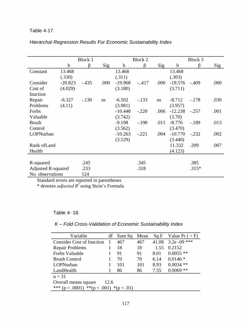
117
Table 4-17.
Hierarchal Regression Results For Economic Sustainability Index
Block 1 Block 2 Block 3
b β Sig b β Sig b β Sig
Constant 13.468
(.330)
13.468
(.311)
13.468
(.303)
Consider
Cost of
Inaction
-20.823
(4.029)
-.435
.000 -19.968
(3.180)
-..417
.000 -19.576
(3.711)
-.409
.000
Repair
Problems
-6.327
(4.11)
-.130
ns -6.502
(3.981)
-.133
ns -8.712
(3.957)
-.178
.030
Forbs
Valuable
-10.448
(3.742)
-.220
.006 -12.238
(3.70)
-.257
.001
Brush
Control
-9.198
(3.562)
-.198
.011 -8.776
(3.470)
-.189
.013
LOPNurban -10.263
(3.529)
-.221
.004 -10.770
(3.440)
-.232
.002
Rank ofLand
Health
11.332
(4.123)
.209
.007
R-squared .245 .345 .385
Adjusted R-squared .233 .318 .315*
No. observations 124
Standard errors are reported in parentheses
* denotes adjusted R2 using Stein‘s Formula
Table 4- 18. K – Fold Cross-Validation of Economic Sustainability Index
Variable df Sum Sq Mean Sq F Value Pr ( > F)
Consider Cost of Inaction 1 467 467 41.08 3.2e -09 ***
Repair Problems 1 18 18 1.55 0.2152
Forbs Valuable 1 91 91 8.01 0.0055 **
Brush Control 1 70 70 6.14 0.0146 *
LOPNurban 1 101 101 8.93 0.0034 **
LandHealth 1 86 86 7.55 0.0069 **
n = 31
Overall means square 12.6
*** (p < .0001) **(p < .001) *(p < .01)
118
Economic sustainability index scores were regressed on land management philosophy
variables identified as the best model after cross-validation, using hierarchical regression
analysis (Table 4-19). The five predictors from BMA Economic Sustainability Index, model 1,
accounted for just under over 1/3 of the variance in economic sustainability index scores in the
final model (R2 = .360; adjusted R2
= .304; F(5,118) = 12.212; p < .001), which was significant
(p < .05). Therefore, the model is considered significantly better than would be expected by
chance thus the null hypothesis of no linear relationship of y to the independents is rejected.
The hierarchical regression model was checked for correlations between the predictors
(Table 4-20). Finding none, Variance Inflation Factor (VIF) values were found to be below 10
as well as noticing tolerance values well above .2; ranging from .882through .989 (Table 4-21).
These facts indicate that multicollinearity is not an issue. Neither was homoscedasticity, as
indicated by the Durban-Watson test (2009). Values less than 1 or greater than 3 are cause for
concern (Field, 2005).
The histogram of the standardized residual values was produced (Figure 4-12). It is as
expected, close to normally distributed around a mean of zero. Also the The Normal Probability
Plot (Figure 4-13) of Regression Standardized Residual values was computed. The plotting of
points very near the reference line indicates little deviation of expected values from observed
values.
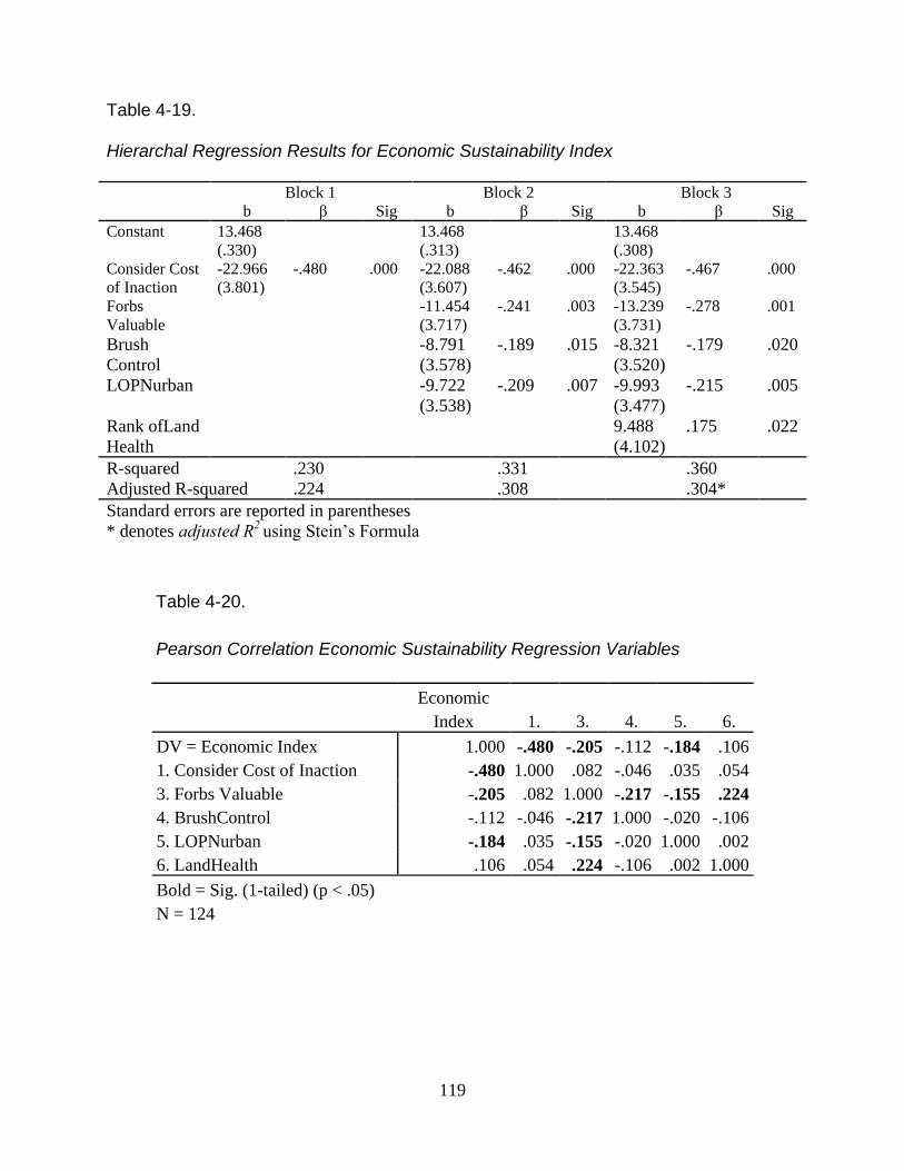
119
Table 4-19. Hierarchal Regression Results for Economic Sustainability Index Block 1 Block 2 Block 3
b β Sig b β Sig b β Sig
Constant 13.468
(.330)
13.468
(.313)
13.468
(.308)
Consider Cost
of Inaction
-22.966
(3.801)
-.480
.000 -22.088
(3.607)
-.462
.000 -22.363
(3.545)
-.467
.000
Forbs
Valuable
-11.454
(3.717)
-.241
.003 -13.239
(3.731)
-.278
.001
Brush
Control
-8.791
(3.578)
-.189
.015 -8.321
(3.520)
-.179
.020
LOPNurban -9.722
(3.538)
-.209
.007 -9.993
(3.477)
-.215
.005
Rank ofLand
Health
9.488
(4.102)
.175
.022
R-squared .230 .331 .360
Adjusted R-squared .224 .308 .304*
Standard errors are reported in parentheses
* denotes adjusted R2 using Stein‘s Formula
Table 4-20.
Pearson Correlation Economic Sustainability Regression Variables
Economic
Index 1. 3. 4. 5. 6.
DV = Economic Index 1.000 -.480 -.205 -.112 -.184 .106
1. Consider Cost of Inaction -.480 1.000 .082 -.046 .035 .054
3. Forbs Valuable -.205 .082 1.000 -.217 -.155 .224
4. BrushControl -.112 -.046 -.217 1.000 -.020 -.106
5. LOPNurban -.184 .035 -.155 -.020 1.000 .002
6. LandHealth .106 .054 .224 -.106 .002 1.000
Bold = Sig. (1-tailed) (p < .05)
N = 124
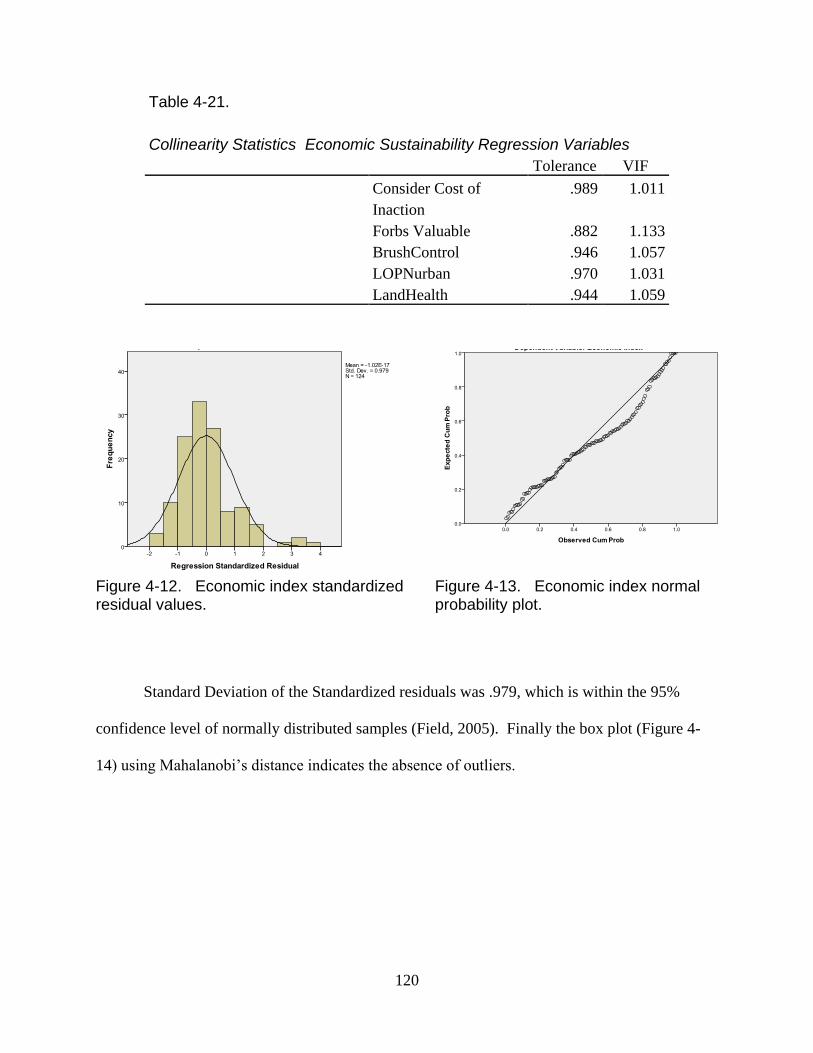
120
Table 4-21.
Collinearity Statistics Economic Sustainability Regression Variables Tolerance VIF
Consider Cost of
Inaction
.989 1.011
Forbs Valuable .882 1.133
BrushControl .946 1.057
LOPNurban .970 1.031
LandHealth .944 1.059
Figure 4-12. Economic index standardized residual values.
Figure 4-13. Economic index normal probability plot.
Standard Deviation of the Standardized residuals was .979, which is within the 95%
confidence level of normally distributed samples (Field, 2005). Finally the box plot (Figure 4-
14) using Mahalanobi‘s distance indicates the absence of outliers.
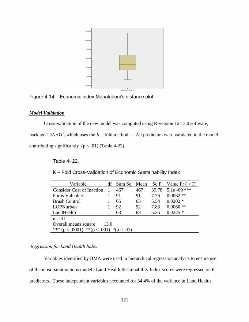
121
Figure 4-14. Economic index Mahalaboni’s distance plot.
Model Validation
Cross-validation of the new model was computed using R-version 12.13.0 software,
package ‗DAAG‘, which uses the K – fold method. . All predictors were validated in the model
contributing significantly (p < .01) (Table 4-22).
Table 4- 22. K – Fold Cross-Validation of Economic Sustainability Index
Variable df Sum Sq Mean Sq F Value Pr ( > F)
Consider Cost of Inaction 1 467 467 39.78 5.1e -09 ***
Forbs Valuable 1 91 91 7.76 0.0062 **
Brush Control 1 65 65 5.54 0.0202 *
LOPNurban 1 92 92 7.83 0.0060 **
LandHealth 1 63 63 5.35 0.0225 *
n = 31
Overall means square 13.0
*** (p < .0001) **(p < .001) *(p < .01)
Regression for Land Health Index
Variables identified by BMA were used in hierarchical regression analysis to ensure use
of the most parsimonious model. Land Health Sustainability Index scores were regressed on 6
predictors. These independent variables accounted for 34.4% of the variance in Land Health
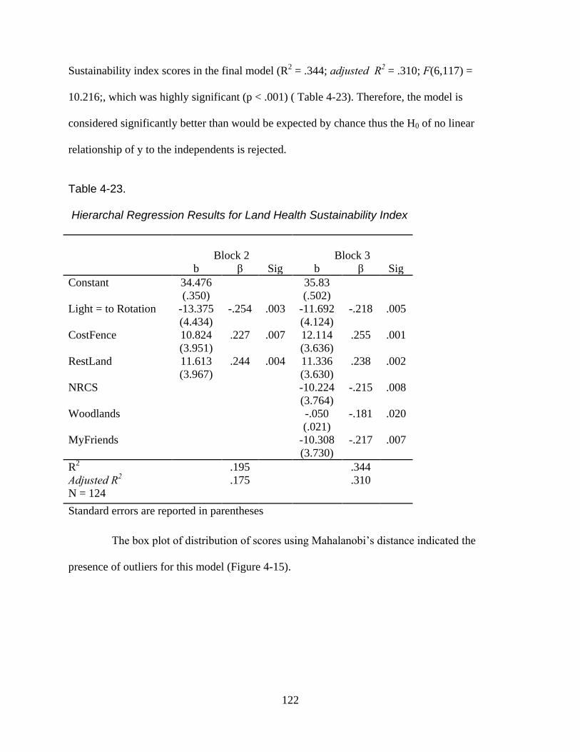
122
Sustainability index scores in the final model (R2 = .344; adjusted R2
= .310; F(6,117) =
10.216;, which was highly significant (p < .001) ( Table 4-23). Therefore, the model is
considered significantly better than would be expected by chance thus the H0 of no linear
relationship of y to the independents is rejected.
Table 4-23. Hierarchal Regression Results for Land Health Sustainability Index
Block 2 Block 3
b β Sig b β Sig
Constant 34.476
(.350)
35.83
(.502)
Light = to Rotation -13.375
(4.434)
-.254
.003 -11.692
(4.124)
-.218
.005
CostFence 10.824
(3.951)
.227
.007 12.114
(3.636)
.255
.001
RestLand 11.613
(3.967)
.244
.004 11.336
(3.630)
.238
.002
NRCS -10.224
(3.764)
-.215
.008
Woodlands -.050
(.021)
-.181 .020
MyFriends -10.308
(3.730)
-.217
.007
R2 .195 .344
Adjusted R2 .175 .310
N = 124
Standard errors are reported in parentheses
The box plot of distribution of scores using Mahalanobi‘s distance indicated the
presence of outliers for this model (Figure 4-15).
123
Figure 4-15. Box Plot of Mahalaboni’s distance scores for land health index.
In an effort to determine the severity of the outliers, the criterion suggested by Field
(2005) was enacted. Seven outliers were identified. Severity of influence was analyzed using
DFFit statistics DFFit statistics (Table 4-24) which should tend toward zero if outliers are not a
significant threat. DFFit is the difference between the predicted value for a case when the model
is calculated including that case and when the model is calculated excluding that case (Field,
2005).
Table 4-24. Dffit Statistic For Land Health Mahalaboni’s Distance Scores
Case DFFit Standardized DFFit
108 -.33582 -.27260
96 .21959 .14435
79 .02889 .01862
67 .22950 .18063
22 -.64889 -.50695
11 .36757 .27565
9 .17838 .13599
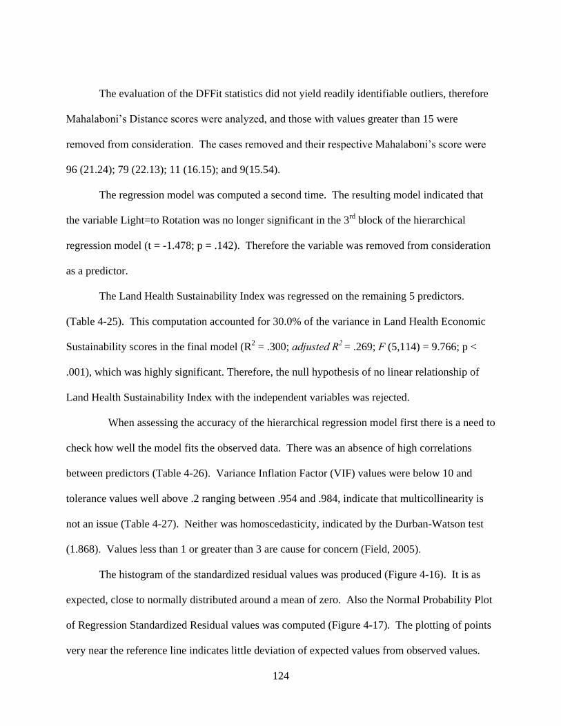
124
The evaluation of the DFFit statistics did not yield readily identifiable outliers, therefore
Mahalaboni‘s Distance scores were analyzed, and those with values greater than 15 were
removed from consideration. The cases removed and their respective Mahalaboni‘s score were
96 (21.24); 79 (22.13); 11 (16.15); and 9(15.54).
The regression model was computed a second time. The resulting model indicated that
the variable Light=to Rotation was no longer significant in the 3rd
block of the hierarchical
regression model (t = -1.478; p = .142). Therefore the variable was removed from consideration
as a predictor.
The Land Health Sustainability Index was regressed on the remaining 5 predictors.
(Table 4-25). This computation accounted for 30.0% of the variance in Land Health Economic
Sustainability scores in the final model (R2 = .300; adjusted R2
= .269; F (5,114) = 9.766; p <
.001), which was highly significant. Therefore, the null hypothesis of no linear relationship of
Land Health Sustainability Index with the independent variables was rejected.
When assessing the accuracy of the hierarchical regression model first there is a need to
check how well the model fits the observed data. There was an absence of high correlations
between predictors (Table 4-26). Variance Inflation Factor (VIF) values were below 10 and
tolerance values well above .2 ranging between .954 and .984, indicate that multicollinearity is
not an issue (Table 4-27). Neither was homoscedasticity, indicated by the Durban-Watson test
(1.868). Values less than 1 or greater than 3 are cause for concern (Field, 2005).
The histogram of the standardized residual values was produced (Figure 4-16). It is as
expected, close to normally distributed around a mean of zero. Also the Normal Probability Plot
of Regression Standardized Residual values was computed (Figure 4-17). The plotting of points
very near the reference line indicates little deviation of expected values from observed values.
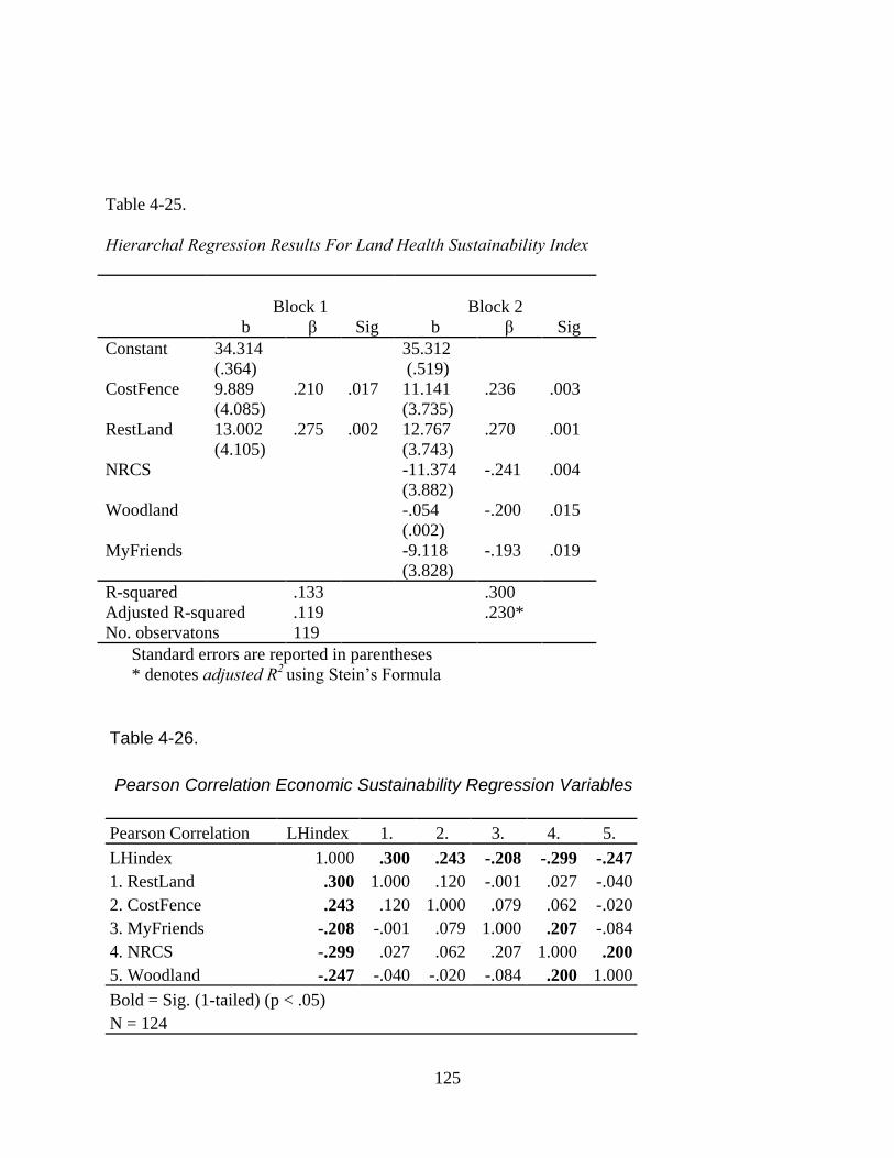
125
Table 4-25.
Hierarchal Regression Results For Land Health Sustainability Index
Block 1 Block 2
b β Sig b β Sig
Constant 34.314
(.364)
35.312
(.519)
CostFence 9.889
(4.085)
.210
.017 11.141
(3.735)
.236
.003
RestLand 13.002
(4.105)
.275
.002 12.767
(3.743)
.270
.001
NRCS -11.374
(3.882)
-.241
.004
Woodland -.054
(.002)
-.200 .015
MyFriends -9.118
(3.828)
-.193 .019
R-squared .133 .300
Adjusted R-squared .119 .230*
No. observatons 119
Standard errors are reported in parentheses
* denotes adjusted R2 using Stein‘s Formula
Table 4-26.
Pearson Correlation Economic Sustainability Regression Variables
Pearson Correlation LHindex 1. 2. 3. 4. 5.
LHindex 1.000 .300 .243 -.208 -.299 -.247
1. RestLand .300 1.000 .120 -.001 .027 -.040
2. CostFence .243 .120 1.000 .079 .062 -.020
3. MyFriends -.208 -.001 .079 1.000 .207 -.084
4. NRCS -.299 .027 .062 .207 1.000 .200
5. Woodland -.247 -.040 -.020 -.084 .200 1.000
Bold = Sig. (1-tailed) (p < .05)
N = 124
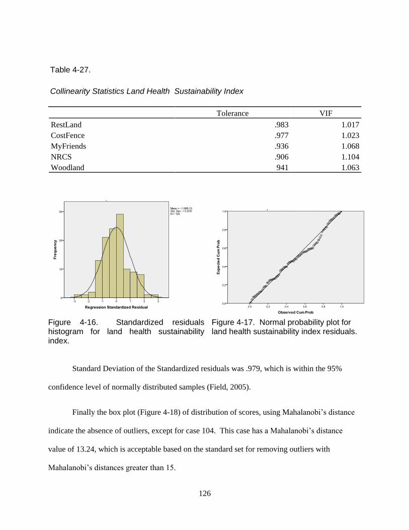
126
Table 4-27.
Collinearity Statistics Land Health Sustainability Index
Tolerance VIF
RestLand .983 1.017
CostFence .977 1.023
MyFriends .936 1.068
NRCS .906 1.104
Woodland 941 1.063
Figure 4-16. Standardized residuals histogram for land health sustainability index.
Figure 4-17. Normal probability plot for land health sustainability index residuals.
Standard Deviation of the Standardized residuals was .979, which is within the 95%
confidence level of normally distributed samples (Field, 2005).
Finally the box plot (Figure 4-18) of distribution of scores, using Mahalanobi‘s distance
indicate the absence of outliers, except for case 104. This case has a Mahalanobi‘s distance
value of 13.24, which is acceptable based on the standard set for removing outliers with
Mahalanobi‘s distances greater than 15.
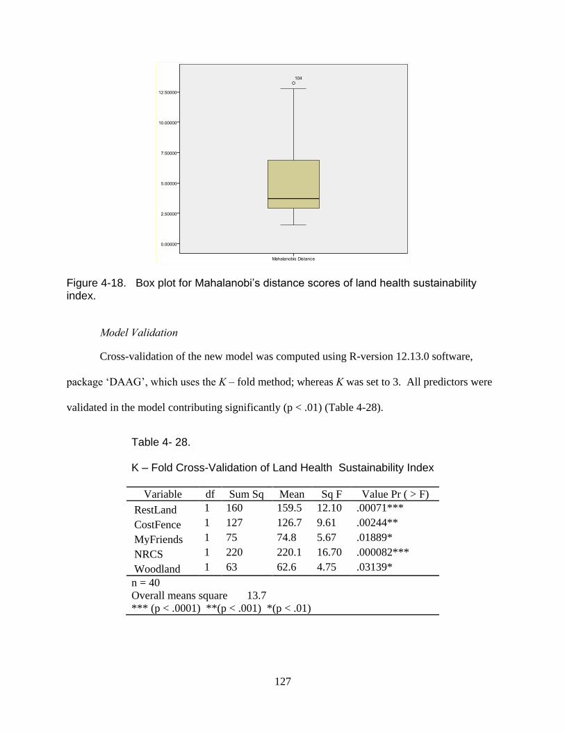
127
Figure 4-18. Box plot for Mahalanobi’s distance scores of land health sustainability index.
Model Validation
Cross-validation of the new model was computed using R-version 12.13.0 software,
package ‗DAAG‘, which uses the K – fold method; whereas K was set to 3. All predictors were
validated in the model contributing significantly (p < .01) (Table 4-28).
Table 4- 28. K – Fold Cross-Validation of Land Health Sustainability Index
Variable df Sum Sq Mean Sq F Value Pr ( > F)
RestLand 1 160 159.5 12.10 .00071***
CostFence 1 127 126.7 9.61 .00244**
MyFriends 1 75 74.8 5.67 .01889*
NRCS 1 220 220.1 16.70 .000082***
Woodland 1 63 62.6 4.75 .03139*
n = 40
Overall means square 13.7
*** (p < .0001) **(p < .001) *(p < .01)
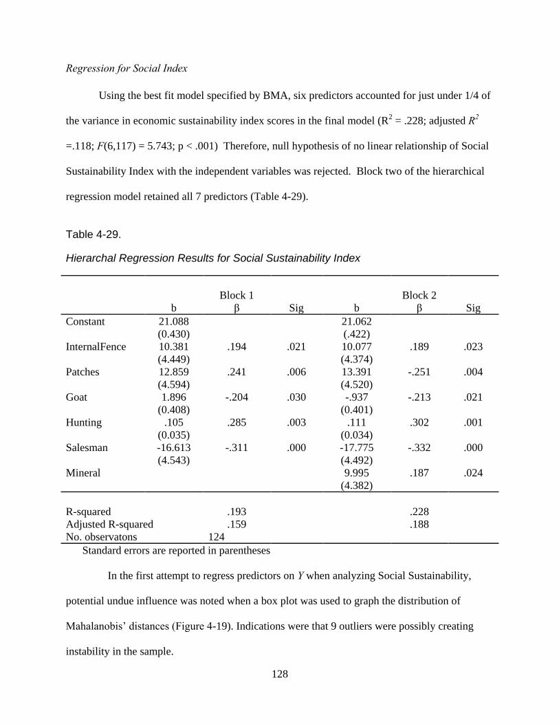
128
Regression for Social Index
Using the best fit model specified by BMA, six predictors accounted for just under 1/4 of
the variance in economic sustainability index scores in the final model (R2 = .228; adjusted R2
=.118; F(6,117) = 5.743; p < .001) Therefore, null hypothesis of no linear relationship of Social
Sustainability Index with the independent variables was rejected. Block two of the hierarchical
regression model retained all 7 predictors (Table 4-29).
Table 4-29.
Hierarchal Regression Results for Social Sustainability Index
Block 1 Block 2
b β Sig b β Sig
Constant 21.088
(0.430)
21.062
(.422)
InternalFence 10.381
(4.449)
.194
.021 10.077
(4.374)
.189
.023
Patches 12.859
(4.594)
.241
.006 13.391
(4.520)
-.251
.004
Goat 1.896
(0.408)
-.204
.030 -.937
(0.401)
-.213
.021
Hunting .105
(0.035)
.285
.003 .111
(0.034)
.302
.001
Salesman -16.613
(4.543)
-.311
.000 -17.775
(4.492)
-.332
.000
Mineral 9.995
(4.382)
.187
.024
R-squared .193 .228
Adjusted R-squared .159 .188
No. observatons 124
Standard errors are reported in parentheses
In the first attempt to regress predictors on Y when analyzing Social Sustainability,
potential undue influence was noted when a box plot was used to graph the distribution of
Mahalanobis‘ distances (Figure 4-19). Indications were that 9 outliers were possibly creating
instability in the sample.
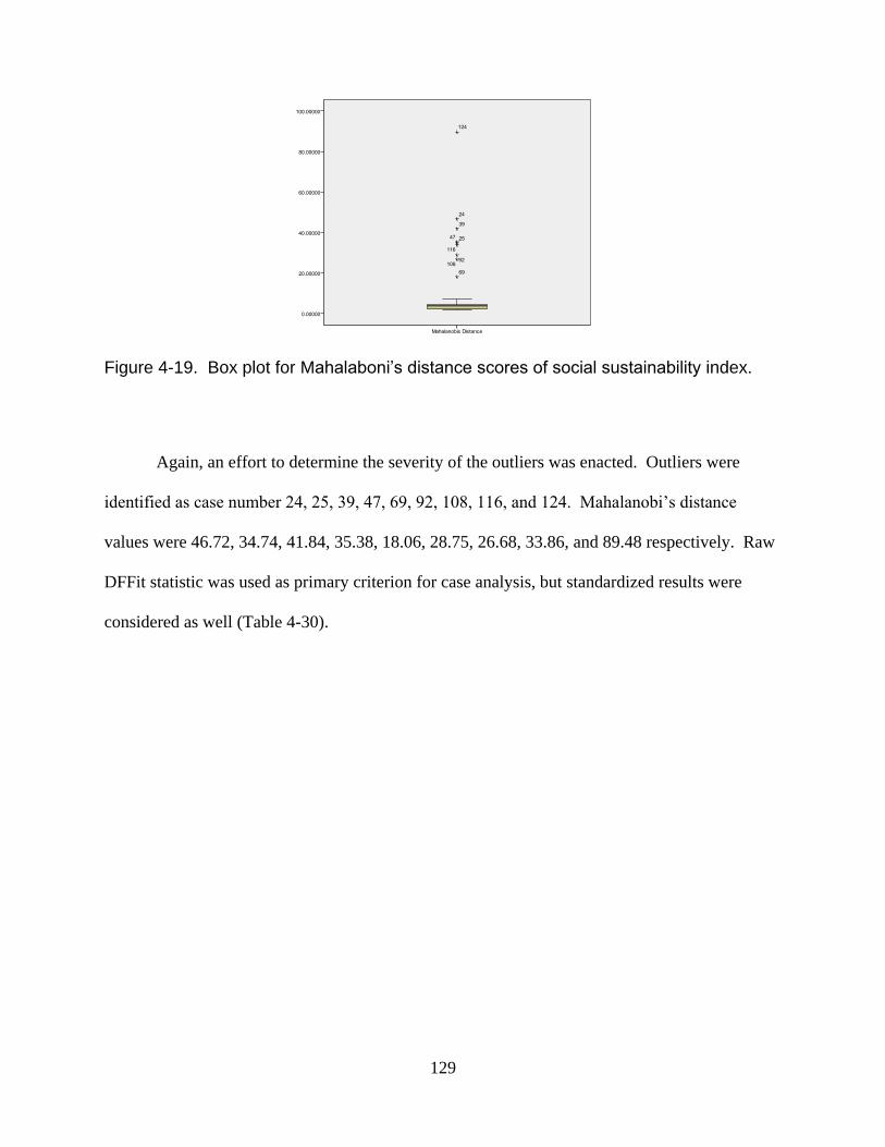
129
Figure 4-19. Box plot for Mahalaboni’s distance scores of social sustainability index.
Again, an effort to determine the severity of the outliers was enacted. Outliers were
identified as case number 24, 25, 39, 47, 69, 92, 108, 116, and 124. Mahalanobi‘s distance
values were 46.72, 34.74, 41.84, 35.38, 18.06, 28.75, 26.68, 33.86, and 89.48 respectively. Raw
DFFit statistic was used as primary criterion for case analysis, but standardized results were
considered as well (Table 4-30).
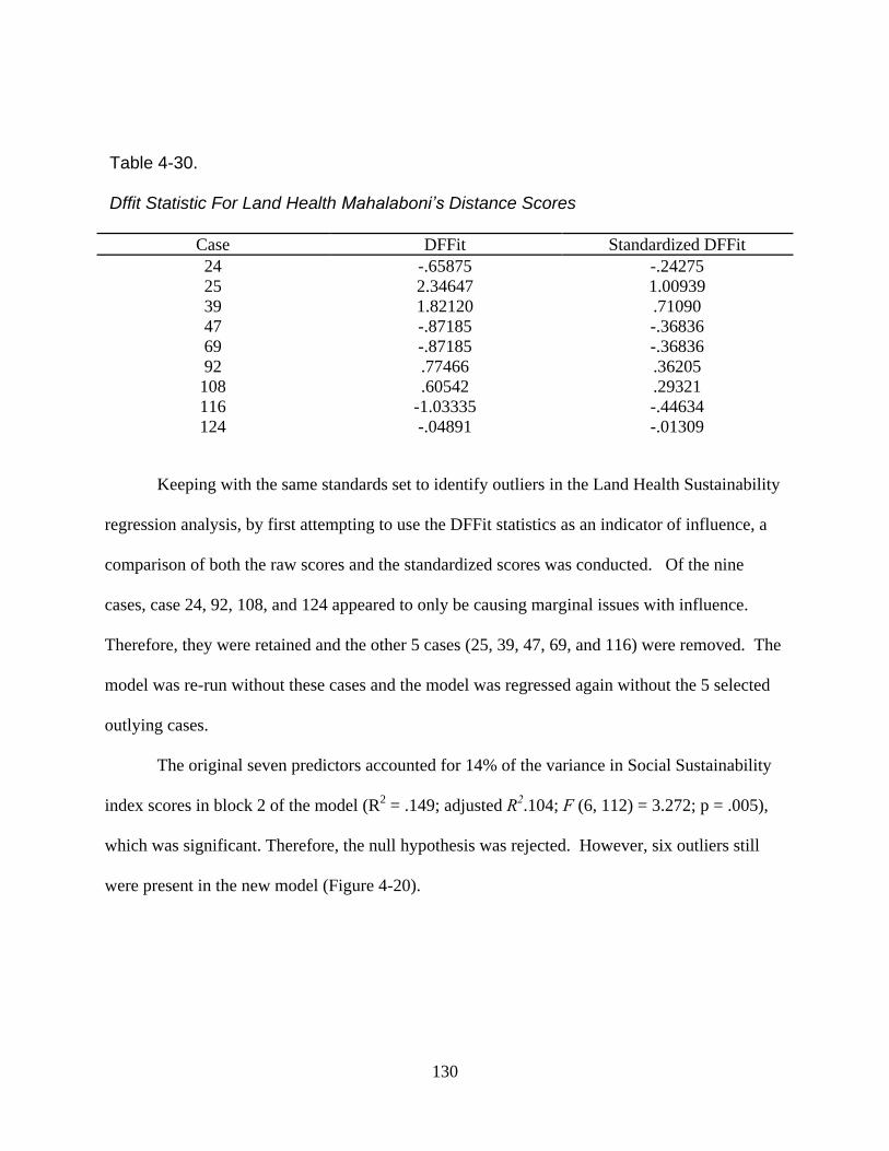
130
Table 4-30. Dffit Statistic For Land Health Mahalaboni’s Distance Scores
Case DFFit Standardized DFFit
24 -.65875 -.24275
25 2.34647 1.00939
39 1.82120 .71090
47 -.87185 -.36836
69 -.87185 -.36836
92 .77466 .36205
108 .60542 .29321
116 -1.03335 -.44634
124 -.04891 -.01309
Keeping with the same standards set to identify outliers in the Land Health Sustainability
regression analysis, by first attempting to use the DFFit statistics as an indicator of influence, a
comparison of both the raw scores and the standardized scores was conducted. Of the nine
cases, case 24, 92, 108, and 124 appeared to only be causing marginal issues with influence.
Therefore, they were retained and the other 5 cases (25, 39, 47, 69, and 116) were removed. The
model was re-run without these cases and the model was regressed again without the 5 selected
outlying cases.
The original seven predictors accounted for 14% of the variance in Social Sustainability
index scores in block 2 of the model (R2 = .149; adjusted R2
.104; F (6, 112) = 3.272; p = .005),
which was significant. Therefore, the null hypothesis was rejected. However, six outliers still
were present in the new model (Figure 4-20).
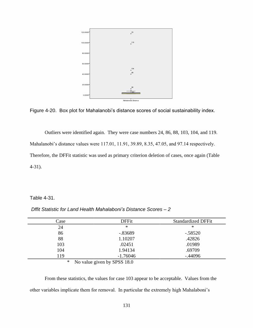
131
Figure 4-20. Box plot for Mahalanobi’s distance scores of social sustainability index.
Outliers were identified again. They were case numbers 24, 86, 88, 103, 104, and 119.
Mahalanobi‘s distance values were 117.01, 11.91, 39.89, 8.35, 47.05, and 97.14 respectively.
Therefore, the DFFit statistic was used as primary criterion deletion of cases, once again (Table
4-31).
Table 4-31. Dffit Statistic for Land Health Mahalaboni’s Distance Scores – 2
Case DFFit Standardized DFFit
24 * *
86 -.83689 -.58520
88 1.10207 .42826
103 .02451 .01989
104 1.94134 .69709
119 -1.76046 -.44096
* No value given by SPSS 18.0
From these statistics, the values for case 103 appear to be acceptable. Values from the
other variables implicate them for removal. In particular the extremely high Mahalaboni‘s
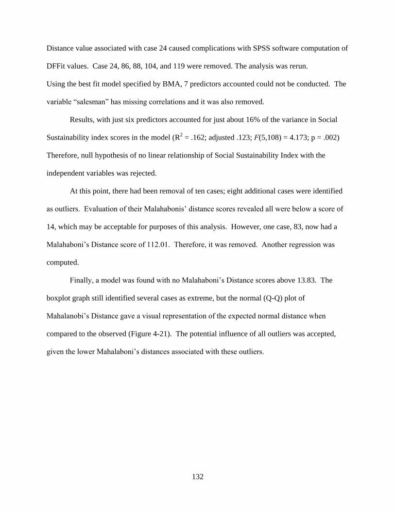
132
Distance value associated with case 24 caused complications with SPSS software computation of
DFFit values. Case 24, 86, 88, 104, and 119 were removed. The analysis was rerun.
Using the best fit model specified by BMA, 7 predictors accounted could not be conducted. The
variable ―salesman‖ has missing correlations and it was also removed.
Results, with just six predictors accounted for just about 16% of the variance in Social
Sustainability index scores in the model (R2 = .162; adjusted .123; F(5,108) = 4.173; p = .002)
Therefore, null hypothesis of no linear relationship of Social Sustainability Index with the
independent variables was rejected.
At this point, there had been removal of ten cases; eight additional cases were identified
as outliers. Evaluation of their Malahabonis‘ distance scores revealed all were below a score of
14, which may be acceptable for purposes of this analysis. However, one case, 83, now had a
Malahaboni‘s Distance score of 112.01. Therefore, it was removed. Another regression was
computed.
Finally, a model was found with no Malahaboni‘s Distance scores above 13.83. The
boxplot graph still identified several cases as extreme, but the normal (Q-Q) plot of
Mahalanobi‘s Distance gave a visual representation of the expected normal distance when
compared to the observed (Figure 4-21). The potential influence of all outliers was accepted,
given the lower Mahalaboni‘s distances associated with these outliers.
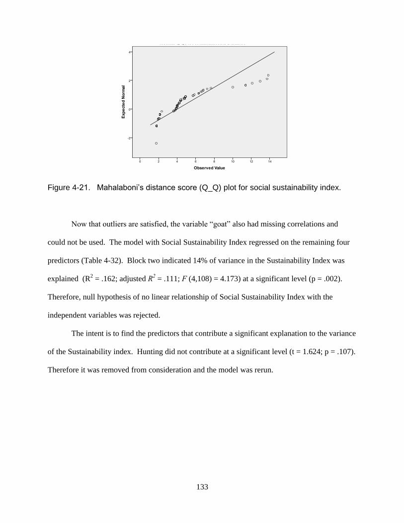
133
Figure 4-21. Mahalaboni’s distance score (Q_Q) plot for social sustainability index.
Now that outliers are satisfied, the variable ―goat‖ also had missing correlations and
could not be used. The model with Social Sustainability Index regressed on the remaining four
predictors (Table 4-32). Block two indicated 14% of variance in the Sustainability Index was
explained (R2 = .162; adjusted R2
= .111; F (4,108) = 4.173) at a significant level (p = .002).
Therefore, null hypothesis of no linear relationship of Social Sustainability Index with the
independent variables was rejected.
The intent is to find the predictors that contribute a significant explanation to the variance
of the Sustainability index. Hunting did not contribute at a significant level (t = 1.624; p = .107).
Therefore it was removed from consideration and the model was rerun.
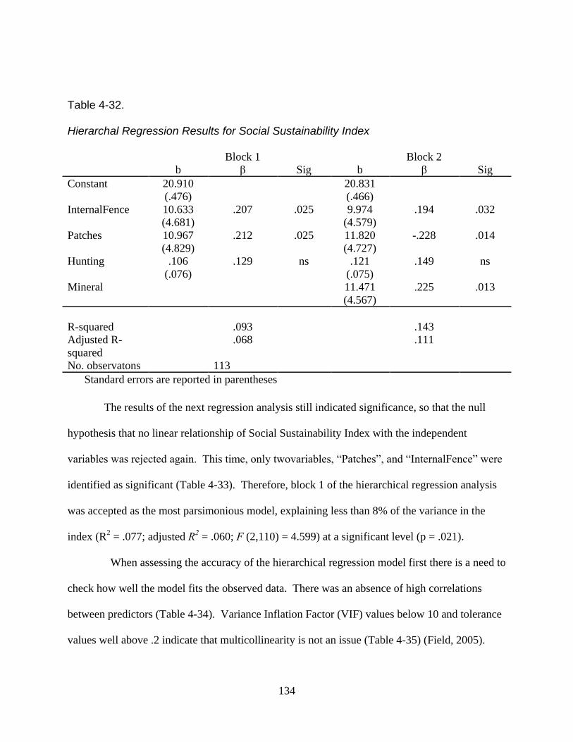
134
Table 4-32. Hierarchal Regression Results for Social Sustainability Index Block 1 Block 2
b β Sig b β Sig
Constant 20.910
(.476)
20.831
(.466)
InternalFence 10.633
(4.681)
.207
.025 9.974
(4.579)
.194
.032
Patches 10.967
(4.829)
.212
.025 11.820
(4.727)
-.228
.014
Hunting .106
(.076)
.129
ns .121
(.075)
.149
ns
Mineral 11.471
(4.567)
.225
.013
R-squared .093 .143
Adjusted R-
squared
.068 .111
No. observatons 113
Standard errors are reported in parentheses
The results of the next regression analysis still indicated significance, so that the null
hypothesis that no linear relationship of Social Sustainability Index with the independent
variables was rejected again. This time, only twovariables, ―Patches‖, and ―InternalFence‖ were
identified as significant (Table 4-33). Therefore, block 1 of the hierarchical regression analysis
was accepted as the most parsimonious model, explaining less than 8% of the variance in the
index (R2 = .077; adjusted R2
= .060; F (2,110) = 4.599) at a significant level (p = .021).
When assessing the accuracy of the hierarchical regression model first there is a need to
check how well the model fits the observed data. There was an absence of high correlations
between predictors (Table 4-34). Variance Inflation Factor (VIF) values below 10 and tolerance
values well above .2 indicate that multicollinearity is not an issue (Table 4-35) (Field, 2005).
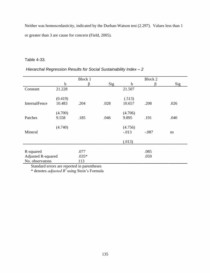
135
Neither was homoscedasticity, indicated by the Durban-Watson test (2.297). Values less than 1
or greater than 3 are cause for concern (Field, 2005).
Table 4-33.
Hierarchal Regression Results for Social Sustainability Index – 2
Block 1 Block 2
b β Sig b β Sig
Constant 21.228
(0.419)
21.507
(.513)
InternalFence 10.483
(4.700)
.204
.028 10.657
(4.706)
.208
.026
Patches 9.558
(4.740)
.185
.046 9.895
(4.756)
.191
.040
Mineral -.013
(.013)
-.087
ns
R-squared .077 .085
Adjusted R-squared .035* .059
No. observatons 113
Standard errors are reported in parentheses
* denotes adjusted R2 using Stein‘s Formula
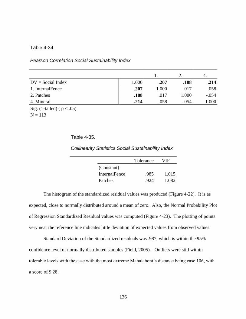
136
Table 4-35.
Collinearity Statistics Social Sustainability Index
Tolerance VIF
(Constant)
InternalFence .985 1.015
Patches .924 1.082
The histogram of the standardized residual values was produced (Figure 4-22). It is as
expected, close to normally distributed around a mean of zero. Also, the Normal Probability Plot
of Regression Standardized Residual values was computed (Figure 4-23). The plotting of points
very near the reference line indicates little deviation of expected values from observed values.
Standard Deviation of the Standardized residuals was .987, which is within the 95%
confidence level of normally distributed samples (Field, 2005). Outliers were still within
tolerable levels with the case with the most extreme Mahalaboni‘s distance being case 106, with
a score of 9.28.
Table 4-34.
Pearson Correlation Social Sustainability Index
1. 2. 4.
DV = Social Index 1.000 .207 .188 .214
1. InternalFence .207 1.000 .017 .058
2. Patches .188 .017 1.000 -.054
4. Mineral .214 .058 -.054 1.000
Sig. (1-tailed) ( p < .05)
N = 113
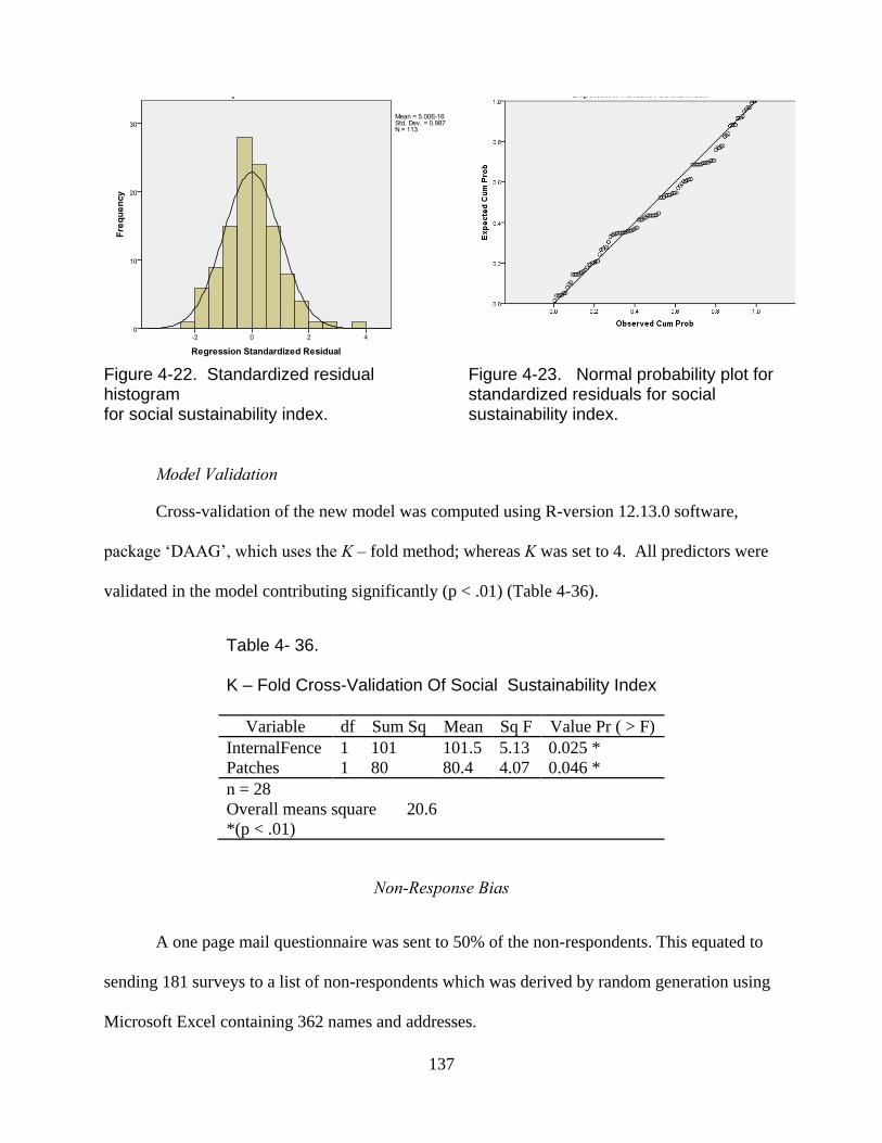
137
Figure 4-22. Standardized residual histogram for social sustainability index.
Figure 4-23. Normal probability plot for standardized residuals for social sustainability index.
Model Validation
Cross-validation of the new model was computed using R-version 12.13.0 software,
package ‗DAAG‘, which uses the K – fold method; whereas K was set to 4. All predictors were
validated in the model contributing significantly (p < .01) (Table 4-36).
Table 4- 36. K – Fold Cross-Validation Of Social Sustainability Index
Variable df Sum Sq Mean Sq F Value Pr ( > F)
InternalFence 1 101 101.5 5.13 0.025 *
Patches 1 80 80.4 4.07 0.046 *
n = 28
Overall means square 20.6
*(p < .01)
Non-Response Bias
A one page mail questionnaire was sent to 50% of the non-respondents. This equated to
sending 181 surveys to a list of non-respondents which was derived by random generation using
Microsoft Excel containing 362 names and addresses.
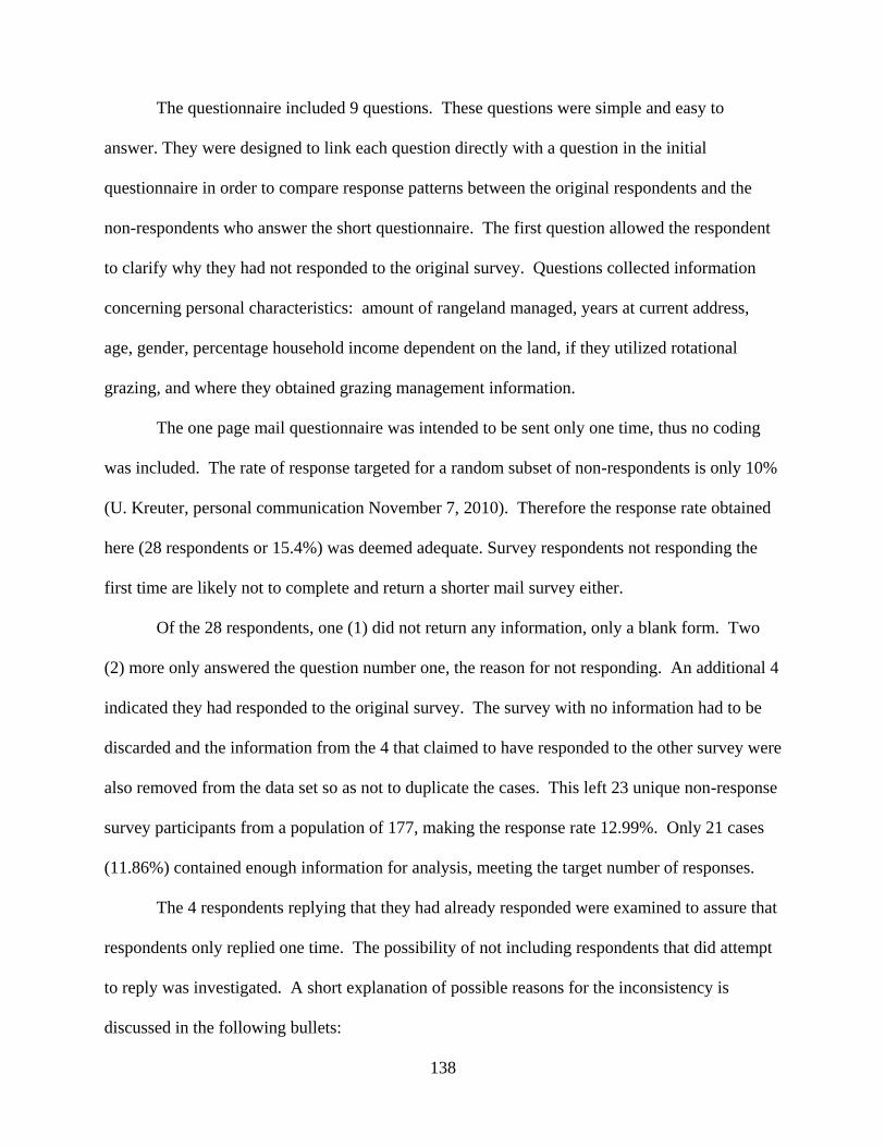
138
The questionnaire included 9 questions. These questions were simple and easy to
answer. They were designed to link each question directly with a question in the initial
questionnaire in order to compare response patterns between the original respondents and the
non-respondents who answer the short questionnaire. The first question allowed the respondent
to clarify why they had not responded to the original survey. Questions collected information
concerning personal characteristics: amount of rangeland managed, years at current address,
age, gender, percentage household income dependent on the land, if they utilized rotational
grazing, and where they obtained grazing management information.
The one page mail questionnaire was intended to be sent only one time, thus no coding
was included. The rate of response targeted for a random subset of non-respondents is only 10%
(U. Kreuter, personal communication November 7, 2010). Therefore the response rate obtained
here (28 respondents or 15.4%) was deemed adequate. Survey respondents not responding the
first time are likely not to complete and return a shorter mail survey either.
Of the 28 respondents, one (1) did not return any information, only a blank form. Two
(2) more only answered the question number one, the reason for not responding. An additional 4
indicated they had responded to the original survey. The survey with no information had to be
discarded and the information from the 4 that claimed to have responded to the other survey were
also removed from the data set so as not to duplicate the cases. This left 23 unique non-response
survey participants from a population of 177, making the response rate 12.99%. Only 21 cases
(11.86%) contained enough information for analysis, meeting the target number of responses.
The 4 respondents replying that they had already responded were examined to assure that
respondents only replied one time. The possibility of not including respondents that did attempt
to reply was investigated. A short explanation of possible reasons for the inconsistency is
discussed in the following bullets:
139
Obvious complications could arise from returns being lost in the mail, or lost during
transport. Returned questionnaires were handled by the University post office, the
administrative personnel at the Institute of Applied Science at UNT and by this
researcher.
There were two (2) instances of returned questionnaires with the unique coding
removed. This action could have been intentional or an inadvertent result from the
respondent removing the cover page during their response or prior to returning. One
of these cases was received after the first mailing of the questionnaire and one after
the second mailing of the questionnaire. Therefore, they were visually evaluated for
similarities. Finding none, they were both used during the analysis.
A potential respondent could have filled in the survey and not remembered that they
had not mailed it.
A final explanation for respondents to the original survey receiving a nonresponse
questionnaire would be sending multiple surveys to the same household. This is
possible, while every effort was made to eliminate the possibility of sending multiple
surveys to the same person, one must consider the original data set. The set was
obtained from the local tax appraisal offices. One person, or household, with
separate land holdings greater than 500 acres would be returned as two or more cases
as long as the name on the tax offices list had any differences at all. This included
different addresses (e.g. a post office box vs. a rural mailbox), different names (e.g. a
land holding owned by one spouse vs. a land holding in both spouses names; or a
landholding listing the same owner with different versions of the same name – one
using the middle initial. one without the middle initial or one holding in the
individuals name and one in a farm name).
Of the 21 remaining surveys, the reasons for not responding varied. One person checked 4
reasons for not responding. Everyone else checked only 1. Reason for not responding, with the
number choosing that reason, is as follows:
Did not receive survey – 0
Did not believe the survey was really anonymous – 1
Did not pertain to me – 1
Lack of time – 8
Survey was too long – 2
Chose not to participate – 5
Other – 6
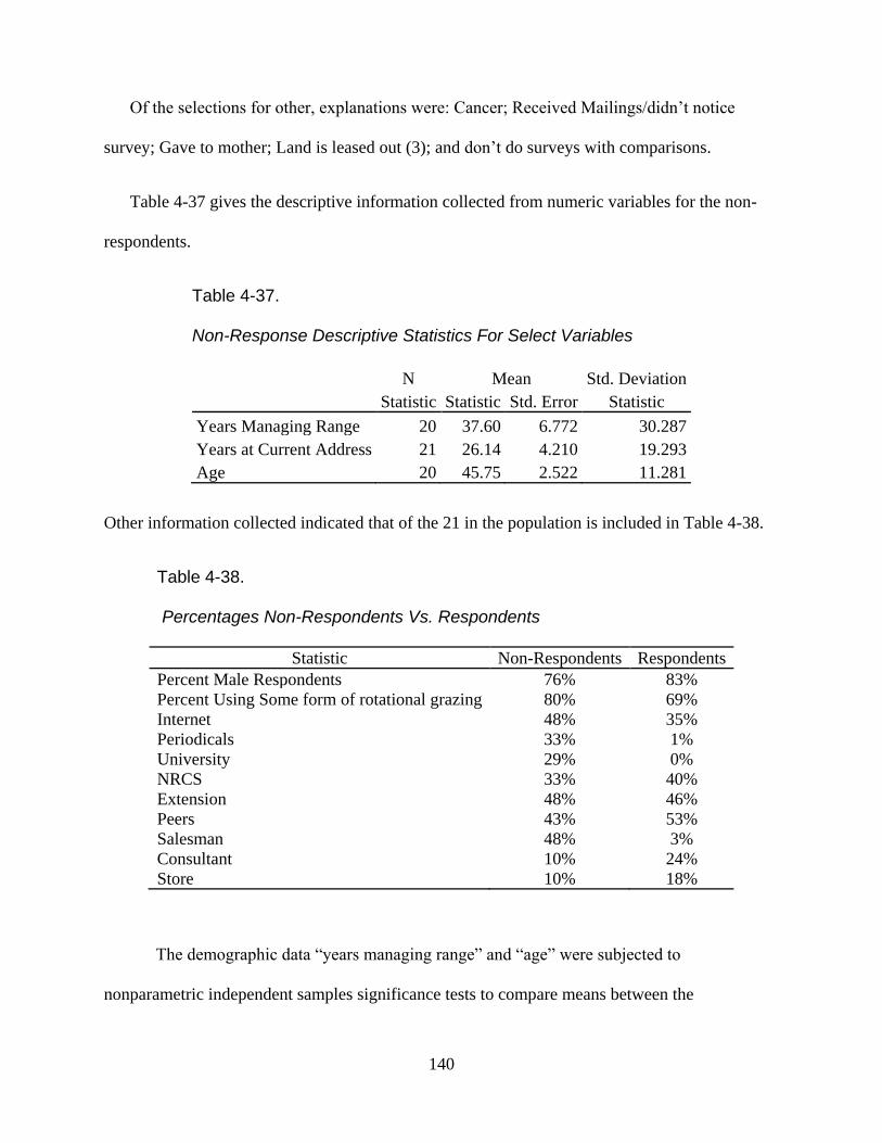
140
Of the selections for other, explanations were: Cancer; Received Mailings/didn‘t notice
survey; Gave to mother; Land is leased out (3); and don‘t do surveys with comparisons.
Table 4-37 gives the descriptive information collected from numeric variables for the non-
respondents.
Table 4-37. Non-Response Descriptive Statistics For Select Variables
N Mean Std. Deviation
Statistic Statistic Std. Error Statistic
Years Managing Range 20 37.60 6.772 30.287
Years at Current Address 21 26.14 4.210 19.293
Age 20 45.75 2.522 11.281
Other information collected indicated that of the 21 in the population is included in Table 4-38.
Table 4-38. Percentages Non-Respondents Vs. Respondents
Statistic Non-Respondents Respondents
Percent Male Respondents 76% 83%
Percent Using Some form of rotational grazing 80% 69%
Internet 48% 35%
Periodicals 33% 1%
University 29% 0%
NRCS 33% 40%
Extension 48% 46%
Peers 43% 53%
Salesman 48% 3%
Consultant 10% 24%
Store 10% 18%
The demographic data ―years managing range‖ and ―age‖ were subjected to
nonparametric independent samples significance tests to compare means between the
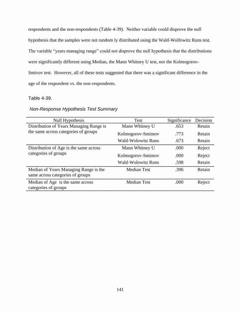
141
respondents and the non-respondents (Table 4-39). Neither variable could disprove the null
hypothesis that the samples were not random ly distributed using the Wald-Wolfowitz Runs test.
The variable ―years managing range‖ could not disprove the null hypothesis that the distributions
were significantly different using Median, the Mann Whitney U test, nor the Kolmogorov-
Smivov test. However, all of these tests suggested that there was a significant difference in the
age of the respondent vs. the non-respondents.
Table 4-39. Non-Response Hypothesis Test Summary
Null Hypothesis Test Significance Decision
Distribution of Years Managing Range is
the same across categories of groups
Mann Whitney U .653 Retain
Kolmogorov-Smimov .773 Retain
Wald-Wolowitz Runs .673 Retain
Distribution of Age is the same across
categories of groups
Mann Whitney U .000 Reject
Kolmogorov-Smimov .000 Reject
Wald-Wolowitz Runs .598 Retain
Median of Years Managing Range is the
same across categories of groups
Median Test .396 Retain
Median of Age is the same across
categories of groups
Median Test .000 Reject
142
CHAPTER V
SUMMARY
This summary begins with useful information for interpretation of the results. Then three
separate sections discuss the findings from the regression analyses. The sections are separated
based on results which aid in assessing economic, environmental and social sustainability for
rangeland in North Central Texas. Each section first describes the indices which is the
dependent variable for the regression analysis and is representative of one part of rangeland
sustainability. Then the meaning of the relationship of each predictor is discussed. Finally,
conclusions are drawn about the results of each model.
After the statistical conclusions, the findings are compared to the original hypotheses
formulated prior to initiation of the study. Then there is a discussion of how these findings
compare to the general study objectives and what implications they may have in effecting
rangeland sustainability. Continuing next, there are acknowledgements of study limitations and
implications for future research. Finally, a conclusion is drawn.
Interpretation of Regression Results
A thorough understanding of the predictors and the direction of the relationship with the
sustainability indices is key to understanding the results of this study. It is important to
remember that the original data, used for the predictors, was transformed using optimal scaling
with the LINEALS approach, using the R package ‗aspect‘. With this approach, transformations
occurred which changed the interpretation of the results. These transformations reversed the
direction of the original coding for some predictors. This was caused because the LINEALS
approach may ―flip‖ the original variable input when it transforms the data to make it more
linearly related (Starkweather, personal communication, July 18, 2011).
143
The LINEALS approach makes transformations which minimize the sum of differences
between the correlation ratios and the squared correlation coefficients on each variable
separately. The LINEALS output was a data matrix, which was optimally scored and could be
used for subsequent analysis (Mair, and de Leeuw, 2008). The computed data matrix made
comparisons between differing types of variables achievable (e.g. dichotomous and Likert
Scale). Since such a re-expression is better suited for further analysis than the original data, that
re-expression was used (de Leeuw, 1988).
Because of the ability of the optimal scaling process to flip the original variable scores,
interpretation of the subsequent analysis must be done carefully. Optimal scaling to achieve
bilinearization with LINEALS will have the effect of transposing the direction of the original
coding for some of the variables, but not all; whereas ―aspect-based techniques
“unstrain" the distribution by finding the inverse transformations, for some families of data, which
makes the distribution of the variables multinormal (Mair, and de Leeuw, 2008). It is apparent
that the transformation must be examined in relation to the original variable coding to understand
the direction (positive or negative) of the relationship between predictors and the dependent
variable with multivariate regression analysis. Therefore, optimal scaling transformations will
be examined for each predictor of the 3 sustainability models investigated in this study. Category
scores, which are available as output from LINEALS, reveals this relationship.
Table 5-1, 5-2, and 5-3 identify each of the predictors, indicate positive or negative
association with the applicable index, describe the original question, the effect of the optimal
scaling process on the original variables and offers rationale suggested by the direction of the
relationship with the index.
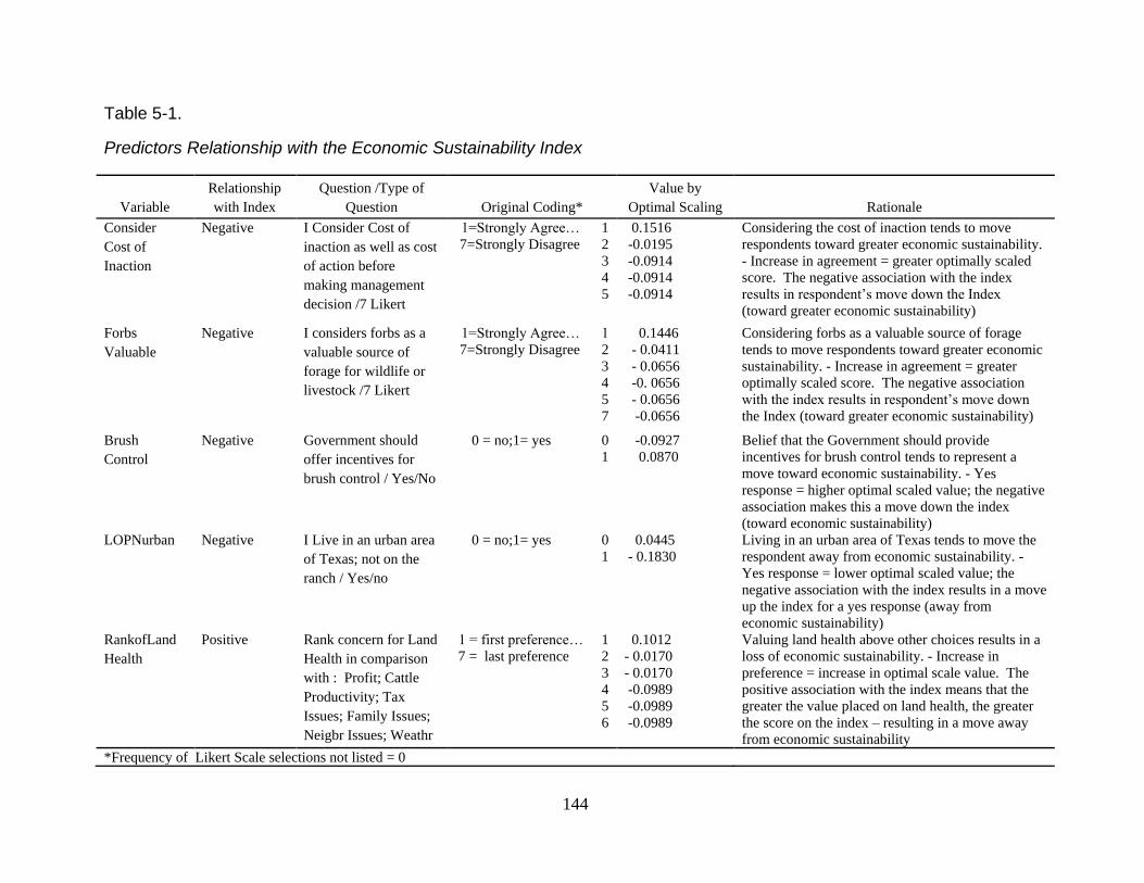
144
Table 5-1.
Predictors Relationship with the Economic Sustainability Index
Variable
Relationship
with Index
Question /Type of
Question Original Coding*
Value by
Optimal Scaling Rationale
Consider
Cost of
Inaction
Negative I Consider Cost of
inaction as well as cost
of action before
making management
decision /7 Likert
1=Strongly Agree… 1
7=Strongly Disagree 2
3
4
5
0.1516
-0.0195
-0.0914
-0.0914
-0.0914
Considering the cost of inaction tends to move
respondents toward greater economic sustainability.
- Increase in agreement = greater optimally scaled
score. The negative association with the index
results in respondent‘s move down the Index
(toward greater economic sustainability)
Forbs
Valuable
Negative I considers forbs as a
valuable source of
forage for wildlife or
livestock /7 Likert
1=Strongly Agree… 1
7=Strongly Disagree 2
3
4
5
7
0.1446
- 0.0411
- 0.0656
-0. 0656
- 0.0656
-0.0656
Considering forbs as a valuable source of forage
tends to move respondents toward greater economic
sustainability. - Increase in agreement = greater
optimally scaled score. The negative association
with the index results in respondent‘s move down
the Index (toward greater economic sustainability)
Brush
Control
Negative Government should
offer incentives for
brush control / Yes/No
0 = no;1= yes 0
1
-0.0927
0.0870
Belief that the Government should provide
incentives for brush control tends to represent a
move toward economic sustainability. - Yes
response = higher optimal scaled value; the negative
association makes this a move down the index
(toward economic sustainability)
LOPNurban Negative I Live in an urban area
of Texas; not on the
ranch / Yes/no
0 = no;1= yes 0
1
0.0445
- 0.1830
Living in an urban area of Texas tends to move the
respondent away from economic sustainability. -
Yes response = lower optimal scaled value; the
negative association with the index results in a move
up the index for a yes response (away from
economic sustainability)
RankofLand
Health
Positive Rank concern for Land
Health in comparison
with : Profit; Cattle
Productivity; Tax
Issues; Family Issues;
Neigbr Issues; Weathr
1 = first preference… 1
7 = last preference 2
3
4
5
6
0.1012
- 0.0170
- 0.0170
-0.0989
-0.0989
-0.0989
Valuing land health above other choices results in a
loss of economic sustainability. - Increase in
preference = increase in optimal scale value. The
positive association with the index means that the
greater the value placed on land health, the greater
the score on the index – resulting in a move away
from economic sustainability
*Frequency of Likert Scale selections not listed = 0
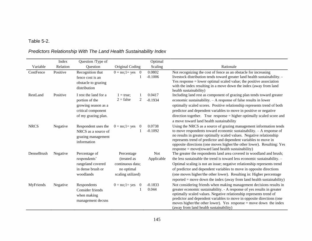
145
Table 5-2.
Predictors Relationship With The Land Health Sustainability Index
Variable
Index
Relation
Question /Type of
Question Original Coding
Optimal
Scaling Rationale
CostFence Positive Recognition that
fence cost is an
obstacle to grazing
distribution
0 = no;1= yes 0
1
0.0802
-0.1006
Not recognizing the cost of fence as an obstacle for increasing
livestock distribution tends toward greater land health sustainability. -
Yes response = lower optimal scaled value; the positive association
with the index resulting in a move down the index (away from land
health sustainability)
RestLand Positive I rest the land for a
portion of the
growing season as a
critical component
of my grazing plan.
1 = true; 1
2 = false 2
0.0417
-0.1934
Including land rest as component of grazing plan tends toward greater
economic sustainability. – A response of false results in lower
optimally scaled scores. Positive relationship represents trend of both
predictor and dependent variables to move in positive or negative
direction together. True response = higher optimally scaled score and
a move toward land health sustainability
NRCS Negative Respondent uses the
NRCS as a source of
grazing management
information
0 = no;1= yes 0
1
0.0738
-0.1092
Using the NRCS as a source of grazing management information tends
to move respondents toward economic sustainability. – A response of
no results in greater optimally scaled values. Negative relationship
represents trend of predictor and dependent variables to move in
opposite directions (one moves higher/the other lower). Resulting: Yes
response = move(toward land health sustainability)
DenseBrush Negative Percentage of
respondents‘
rangeland covered
in dense brush or
woodlands
Percentage
(treated as
continuous data;
no optimal
scaling utilized)
Not
Applicable
The greater the respondents land area covered in woodland and brush;
the less sustainable the trend is toward less economic sustainability. –
Optimal scaling is not an issue; negative relationship represents trend
of predictor and dependent variables to move in opposite directions
(one moves higher/the other lower). Resulting in: Higher percentage
reported = move down the index (away from land health sustainability)
MyFriends Negative Respondents
Consider friends
when making
management decsns
0 = no;1= yes 0
1
-0.1833
0.044
Not considering friends when making management decisions results in
greater economic sustainability. - A response of yes results in greater
optimally scaled values. Negative relationship represents trend of
predictor and dependent variables to move in opposite directions (one
moves higher/the other lower). Yes response = move down the index
(away from land health sustainability)
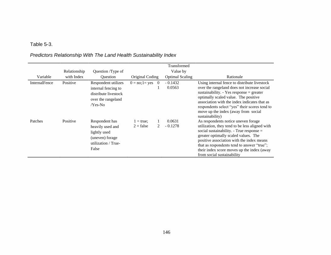
146
Table 5-3.
Predictors Relationship With The Land Health Sustainability Index
Variable
Relationship
with Index
Question /Type of
Question Original Coding
Transformed
Value by
Optimal Scaling Rationale
InternalFence Positive Respondent utilizes
internal fencing to
distribute livestock
over the rangeland
/Yes-No
0 = no;1= yes 0
1
- 0.1432
0.0563
Using internal fence to distribute livestock
over the rangeland does not increase social
sustainability. - Yes response = greater
optimally scaled value. The positive
association with the index indicates that as
respondents select ―yes‖ their scores tend to
move up the index (away from social
sustainability)
Patches Positive Respondent has
heavily used and
lightly used
(uneven) forage
utilization / True-
False
1 = true; 1
2 = false 2
0.0631
- 0.1278
As respondents notice uneven forage
utilization, they tend to be less aligned with
social sustainability. - True response =
greater optimally scaled values. The
positive association with the index means
that as respondents tend to answer ―true‖;
their index score moves up the index (away
from social sustainability
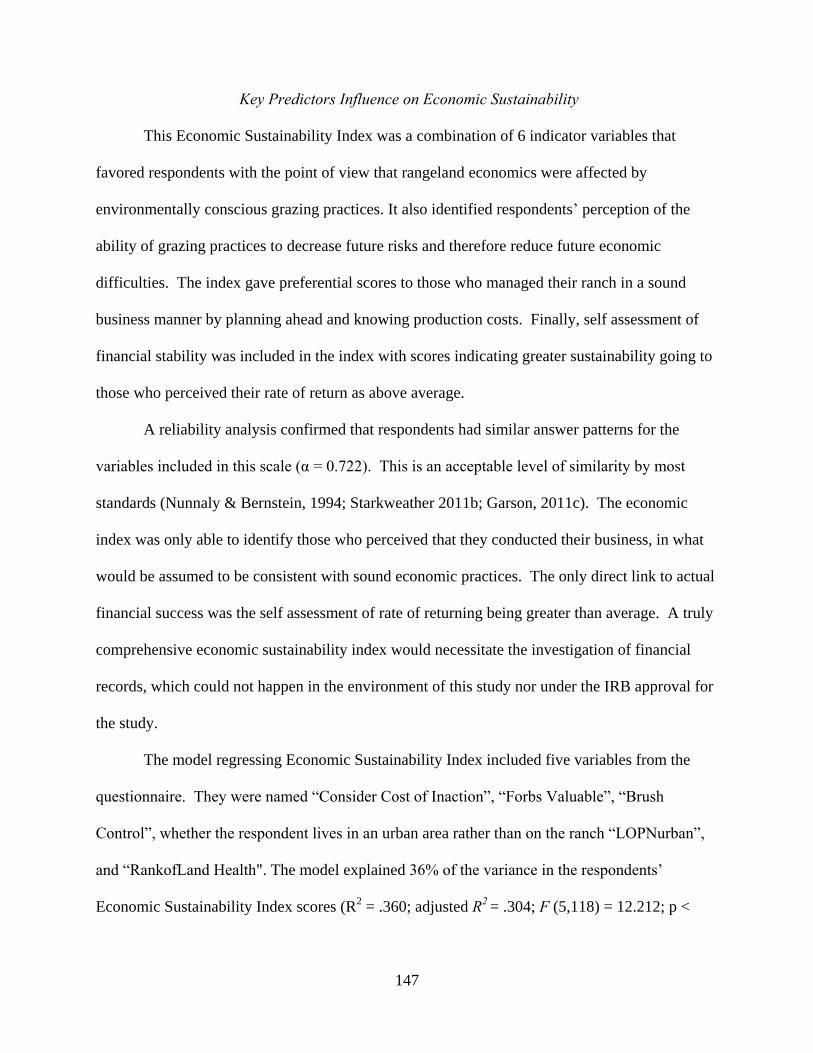
147
Key Predictors Influence on Economic Sustainability
This Economic Sustainability Index was a combination of 6 indicator variables that
favored respondents with the point of view that rangeland economics were affected by
environmentally conscious grazing practices. It also identified respondents‘ perception of the
ability of grazing practices to decrease future risks and therefore reduce future economic
difficulties. The index gave preferential scores to those who managed their ranch in a sound
business manner by planning ahead and knowing production costs. Finally, self assessment of
financial stability was included in the index with scores indicating greater sustainability going to
those who perceived their rate of return as above average.
A reliability analysis confirmed that respondents had similar answer patterns for the
variables included in this scale (α = 0.722). This is an acceptable level of similarity by most
standards (Nunnaly & Bernstein, 1994; Starkweather 2011b; Garson, 2011c). The economic
index was only able to identify those who perceived that they conducted their business, in what
would be assumed to be consistent with sound economic practices. The only direct link to actual
financial success was the self assessment of rate of returning being greater than average. A truly
comprehensive economic sustainability index would necessitate the investigation of financial
records, which could not happen in the environment of this study nor under the IRB approval for
the study.
The model regressing Economic Sustainability Index included five variables from the
questionnaire. They were named ―Consider Cost of Inaction‖, ―Forbs Valuable‖, ―Brush
Control‖, whether the respondent lives in an urban area rather than on the ranch ―LOPNurban‖,
and ―RankofLand Health". The model explained 36% of the variance in the respondents‘
Economic Sustainability Index scores (R2 = .360; adjusted R2
= .304; F (5,118) = 12.212; p <
148
.001). The results show that all predictors in the model were statistically significant in assessing
the variance in economic sustainability for the study population (p < .05).
The standardized model predicting outcome of the Economic Sustainability Index
(adjusted R2 = .195; p < .001) is as follows:
Economic Sustainability Index = -.467(Consider Cost of Inaction) - .278 (Forbs
Valuable) -.179 (Brush Control) -.215(LOPNurban) + .175(Rank ofLand Health)
The economic sustainability index had a negative relationship with variables ―Consider
Cost of Inaction‖. The negative association with the index is explained by the investigating the
relationship between the optimally scaled variable score and the original coding with the index.
The closer to ―1‖ or ―Strongly Agree‖ a respondent‘s answer, the greater the optimal scaling
score. Therefore, as a land manager more strongly agreed with the fact that they considered the
cost of inaction as well as action the negative association with the index resulted in respondent‘s
move down the index (toward greater economic sustainability). In essence when respondents
more strongly agreed with the statement that they considered both the cost of action and the cost
of inaction when making management decisions, they tended to move their economic index score
toward sustainability. These results are consistent with what one may assume a conscientious
land management philosophy may be. Considering inaction equally, with action, would align
with pasture deferment from use at times of greater stress, such as during a drought, which has
land health benefits (Teague et al., 2004). Sullivan (2001) noted that holistic resource
management provides people with a means to make decisions that more accurately mirror the
way nature functions, and thereby ensure that our civilization is truly sustainable over time‖
(Sullivan, 2001). In this case, ―Consider Cost of Inaction‖ also indicates willingness to accept
149
natural processes as a part of the management scheme. Disagreement with this would indicate a
philosophy whereby man can adjust for nature.
Also ―Forbs Valuable‖ had a negative association with the economic index. The
relationship between the optimally scaled score and the original Likert Scale coding are the same
as in the prior example. Therefore, this association is affirmation that respondents who did
consider forbs as a valuable source of forage for livestock and wildlife tended to have more
sustainable scores on the economic index. This indicates that economic sustainability is at least
somewhat aligned with use of diverse enterprises, as domestic goats and sheep are greater
consumers of forbs than cattle (Holechek, 1984). Diverse enterprises could also be described as
multiple species of livestock, wildlife production, wildflower viewing, etc. In general
biodiversity is desirable, and would indicate ecological conscientiousness. This is evident with
findings that indicate the rangeland is best managed for diversity and ecological function under
the watchful eye of the conscious agrarian (Hughes, 1983; Dagget, 1995).
The relationship identified may indicate optimizing opportunity, especially in that of
capitalizing from wildlife resources and recreation whereas hunting, exotic animals, and
recreation resulted in 8.34% of respondent‘s income. However, the use of multiple species of
livestock to enhance sustainability and diversity still appears to be an untapped economic
opportunity. Respondents utilizing sheep or goats enterprises only comprise 0.2% of
respondent‘s income.
A negative relationship was noticed with the variable ―Brush Control‖ and the economic
sustainability index. Optimally scaled values were greater for respondents choosing ―yes‖,
meaning a negative relationship to ―Brush Control‖ would indicate greater Economic
Sustainability; as the optimally scaled value moved up, the index score moved down (toward
sustainability). Therefore, greater economic sustainability was obtained by those agreeing with
150
government providing incentives for brush control. This relationship may be an indication that
government assistance in areas of critical concern, such as brush encroachment, adds stability to
rangeland enterprises, thus moving the respondent toward economic sustainability. It is known
that brush encroachment is expensive in both the cost of control and the cost of lost productivity
(Towne and Ohlenbusch , 1992). This variable being identified as a predictor for economic
sustainability, leads to the belief that the problem of brush encroachment is one that presents
economic strain to ranch managers. Implications are that managers do not have the resources, on
their own accord, to fully deal with this problem. There obviously exists a desire to eliminate
brush from the rangeland. This is also aligned with the native ecological state of the tall grass
prairie. Bakker and Berendse (1999) suggest that the current intensity of agricultural use sets the
rate of recovery for rangeland which has been encroached upon by brush.
The variable ―NOPNurban‖ was a demographic variable added to separate the urban
respondents from rural respondents. Living in an urban area of Texas predicted a less
sustainable index score. A respondent indicating that they lived in an urban area corresponded
with a lower optimal scaled value. Because of the negative association with the index this meant
a response of ―yes‖ caused a move up the index (away from economic sustainability). There are
several theories that could explain this phenomenon. Living in an urban setting would suggest
that ranching may not be the primary source of income for the respondent. Economic
sustainability may not be as important to these respondents as there may be additional income
sources. Without economic incentive an urban resident may be less proactive in their business
procedure, possibly less likely to implement a long-range plan, or know production costs, or hold
a lesser degree of belief that grazing management is influential on economic risk and long-term
economic performance of the ranch. In addition to these theories, Beem (2010) suggests that
151
absentee landowners would incur economic difficulties because they lack knowledge concerning
tenants care for the land.
Valuing land health above 6 other choices resulted in a decline of economic
sustainability. An increase in preference was similarly met with an increase in optimal scale
value. The positive association with the index means that the greater the value placed on land
health, the greater the score on the index – resulting in a move away from economic
sustainability. The positive relationship between the Economic Sustainability index and the
variable ―RankofLand Health‖ indicates a lack of desire for the economically sustainable ranch
to maintain a healthy landscape. Respondents were asked to rank seven things in order of
importance. These were: profit, productivity, land health, tax issues, family issues, neighbor
issues, and weather. The choice of land health was denoted as ―RankofLand Health‖. The
relationship of this predictor with the index indicates that conscious, environmental stewardship
choices and economic sustainability are not aligned in the mind of the respondents.
Most of the predicting variables are philosophic in nature; in fact, three of the variables
came directly from the section 1 of the questionnaire, titled ―Management Philosophy‖. The
other variables identified as predictors are also philosophic in their nature. ―RankofLand
Health‖, which originated in section 5, ―Quality of Life‖, suggests respondents‘ values. It can be
hypothesized that living in an urban area would lead to different values and resulting philosophy
from respondents living in a more rural setting, as indicated by the predictor ―LOPNurban, a
demographic variable from section 6. These facts result in the conclusion that the Economic
Sustainability Index, as calculated within this study is a function of ranchers‘ philosophy, or
mind set.
The results presented here also agree with research that has shown that the traditional
management regarding livestock is as philosophic as it is economic. Attaining philosophic and
152
economic goals outweigh expenses incurred to the environment. Indications are that producers
view cattle ownership as a means to: (1) ensure they are able to continue land ownership; (2) as a
source of security and liquidity, and; (3) as a way of life worthy of passing to the next generation
(Costa and Reham, 2005). These findings are also in alignment with Chouinard et al. (2008),
who found profit-maximizing motivations coincided with valuing environment only to the extent
that it provided direct personal benefits for farmers in Washington State. If nothing else, one
can begin to understand the dilemma between the ―sustainability movement‖ and the rancher.
The sustainability movement tends to focus on land health, where the economically successful
rancher doesn‘t readily recognize the connection. This realization is a confirmation of the
traditional rancher stereotype.
Even with confirmation of the stereotype, the predictors ―Consider Cost of Inaction‖ and
―Forbs Valuable‖ may be identifying the beginning of a shift from these historic trends. Even
though ranchers have not embraced land health has a means of economic sustainability
(indicated by ―Rank of Land Health‖), this study provides a means of qualifying diversity and
natural processes as aligning with economic sustainability. Obviously some ranchers have
begun to recognize this and are implementing these philosophies in their management practices.
Comparison of these philosophies has now revealed alignment with economic benefits. Further
evidence that some adoption of land friendly management has occurred is supported by the
Sustainable Rangeland Roundtable (2005). They stated an examination of rangeland health and
productive capacity, showed that rangeland health, although measured differently over the 20
years, had clearly improved during this time in most regions.
Kreuter et al. (2006) hypothesized that land owners in states with significant areas of
public land might be less resistant to managing land in ways that enhance the delivery of socially
desirable ecosystem services compared to landowners in private land states (such as Texas). The
153
implication was that land managers might be need assurances that private property rights will not
erode as a result of adoption of land management practices that enhance delivery of ecosystem
services on privately owned rangelands. This hypothesis could be expanded to combine the
notion that private land ownership may indirectly include profit maximizing motivations. In
order to motivate landowners to adopt ecosystem friendly practices, it must be demonstrated how
placing value in the environment could provide direct personal benefits like profit maximization.
Again, evidence that this is beginning to occur is reiterated by this study as two predictors
(―Forbs Valuable‖ and ―Brush Control‖) indicating concern for natural processes, and increased
interest in biodiversity are significant predictors for economic sustainability
Rangeland economic sustainability does not appear to be a motivator which would result
in adoption of different management purely for the broad sense of societal or ecological needs.
Instead, in order to motivate landowners to adopt ecosystem friendly practices, it must be
demonstrated how placing value in the environment could provide direct personal benefits like
profit maximization.
The objectives of this study stated a desire to address data gaps and research needs
associated with rangeland sustainability indicators. The predictors for economic sustainability
indicate that valuing land health is not indicative of economic sustainability. Historically, profits
were realized by depleting the range (NRCS, 2000). Further, Leopold (1938) believed over 60
years ago, that the overall societal management system in place was a problem. It was then
driven by governmental policy and by economics. In that atmosphere, it was impossible for
many land managers to implement more ecologically sound practices without the notion of
economic gains. The findings of this study cannot dispute this notion.
This model emphasizes the need for research to address ecology and/or social satisfaction
as an economic resource; specifically there are two suggested actions. First, target education to
154
ranchers where sustainability is addressed in a manner which fosters recognition of direct
benefits to their economic well-being. Secondly, continued investigation of interactions between
land rest and other grazing management variables is necessary to fully understand how to best
deliver education concerning ecological benefits it offers.
Key Predictors Influence on Land Health Sustainability
The Land Health Sustainability index was composed of a series of 16 questions that
asked respondents to identify changes in characteristics of their rangeland as evaluated by the
plant community, the native animal community, land erosion and water infiltration. The 16
questions are assessments of land health indicators which ask for the direction of change, rather
than a direct measurement. This is important given that ecological sites are constantly changing.
Self assessment of land health in this manner is relevant as revealed by Knapp and Fernandez-
Gimenez (2009) when they found that rancher knowledge complemented scientific knowledge in
its ability to provide site-specific information on management practices and ecological responses,
and insight regarding potential indicators of rangeland health. Therefore, this index should be
capable of gauging ecological attributes of a ranch as assessed by Cronbach‘s alpha (α =.710).
The Land Health Sustainability scores were calculated so that greater sustainability was
aligned with a decrease in level of mesquite, juniper, other brush, bare ground, invasive weeds,
livestock trails, gullies, soil compaction, short grass, evidence of elevated rocks or clumps,
evidence of plant litter clinging to grass clumps and stones, and other water flow patterns.
Greater sustainability was indicated by an increase in tall grasses, turkey, quail, other birds, wild
hogs, and deer.
The Land Health Sustainability Index was regressed on 5 predictors CostFence,
RestLand, NRCS, DenseBrush, and MyFriends. This model explained 30% of the variance in
155
Land Health Sustainability Index scores in the final model (R2 = .300; adjusted R2
= .23; (5,114)
= 9.766; p < .001), which was highly significant.
The standardized model predicting outcome of the Economic Sustainability Index is as
follows:
Land Health Sustainability Index =.238(RestLand) - .215(NRCS) + .255(CostFence) -
.181(Woodland) -.217(MyFriends)
When investigating the relationship of the predictors to the Land Health Index, the
predictor ―RestLand‖ had a positive relationship with the index. Given that the optimally scaled
values align with a higher value being place on a response of ―true‖ by the respondents; this
relationship indicates that respondents who are including pasture rest in their grazing
management plan obtain more sustainable scores on the Land Health Sustainability index. This
observation is supported by overwhelming evidence from literature (Smith 1895; Sampson 1913;
Rogler 1951; Scott 1953; Matthews 1954; Merrill 1954; Hormay 1956; Hormay and Evanko
1958; Hormay and Talbot 1961; Hormay 1970; Reardon and Merrill, 1976; Booysen and Tainton
1978; Taylor et al., 1980; Thurow et al., 1988; Taylor et al., 1993; Tainton et al., 1999; Snyman
1998; Teague et al., 2004; Müller et al., 2007;Teague et al., 2011, in press) .
The variable ―CostFence‖ describes the respondent‘s view of the cost of fencing as an
obstacle to increasing livestock distribution on their property. Since the optimally scaled score
is greater for those respondents who indicate that the cost of fence was not an obstacle to
livestock distribution, the positive association with the land health index indicates that a
respondent believing cost of fence is an obstacle is less likely to have a high score on the land
health sustainability index. It would be intuitive that those seeking to rest pastures would
consider additional fencing to increase livestock distribution across their rangeland. This
variable compliments the predictor ―RestLand‖. Not considering the cost of building the fence
156
as an obstacle would indicate that the respondent had the notion that additional fencing was a
management practice they could implement. Therefore, respondents who were able to utilize
more fencing were able to afford each pasture more rest, and therefore, they noticed a change in
their land that is in agreement with greater land sustainability.
The variable ―NRCS is an indicator of where respondents obtain information concerning
grazing management. The Natural Resource Conservation Service (NRCS) is a branch of the
USDA that is designed to recommend management practice that would be in accordance with
grazing management which would conserve natural resources. Investigation of prescribed
grazing guidelines for NRCS personnel are revealed in Section 5.1-2 of the National Range and
Pasture Handbook, (NRCS, 2003). This is a resource for NRCS personnel that addresses
prescribed grazing. It states ―The management objective must meet the needs of the landowner,
the resource, and the grazing animals.‖ The negative relationship observed in this study
indicates that they are accomplishing their purpose. Where one may expect the relationship
between ―NRCS‖ and the land health sustainability index to be positive, the process of optimal
scaling has clouded the issue somewhat. Optimally scaled scores are lower when respondents
indicated they utilized the NRCS as a source of grazing information. As a result the negative
association between the predictor and the index actually indicate that as respondents tended to
utilize information from the NRCS, their resulting Land Health Index moved toward
sustainability.
The negative association with the variable ―DenseBrush‖ and the land health
sustainability index is to be expected. This negative association can be taken at face value, as the
nature of the original coding for the variable ―DenseBrush‖ did not require optimal scaling
procedures. One of the threats to the rangelands includes encroachment of woody plant species
(Maczko and Hidinger, 2008). Specifically, past land use practices have created a landscape that
157
has experienced invasion and domination, in some areas, by problematic brush species (Texas
Parks and Wildlife, 2010). It has been shown that severely degraded rangelands have the
propensity to shift to a stable, shrub-dominated state that will not return their original
composition even with elimination of further grazing (Christensen et al., 2003).
The final variable under consideration is ―MyFriends‖ had a negative relationship with
the Land Health Sustainability Index. Optimal scaling resulted in scores which were greater
when respondents did favor consideration of their friends when making management decisions.
The finding tends to suggest that consideration of one‘s friends would move the respondent‘s
index score away from land health sustainability. While it is difficult to develop a rational
connection between sustainability and this variable, there is more than one possible explanation
for consideration of friends in decision making. First, this consideration may be indicative of a
hobby rancher, or of a ranch manager with little experience and a need for suggestions from a
neighbor. This analysis would be consistent with the predictor ―NRCS‖ being identified earlier.
It is logical that this predictor may be an extension of where information is obtained. Another
explanation would be that the ranch is recreational; ranch management and the ranching
experience are desired to be shared with friends. Yet another explanation could be that it
indicates pride in manager‘s land and therefore, desire to include those close to the manager in
the ranching experience.
It can be ascertained that ―CostFence‖, ―RestLand‖, ―NRCS‖, ―DenseBrush‖ and
―MyFriends‖ are predictors for the land health sustainability index. Results have been shown to
be in agreement with many other sources of literature. The only predictor that leaves any
uncertainty as to understanding the basis of its contribution is ―MyFriends‖, yet an explanation
has been offered. The findings suggest whole-ranch assessment of land health sustainability is
aligned with management philosophies where NRCS recommendations are utilized and friends
158
are not included in the decision making process; where management practices such as additional
fencing is not an obstacle and resting land is a component of the management plan; and where
woody plants are not a major percentage of land characteristics.
Key Predictors Influence on Social Sustainability
The Social Sustainability Index was developed like the others, by maximizing the
variables in the relevant section of the questionnaire for Cronbach‘s alpha coefficient. This
index was derived from Section 5, which was titled Quality of Life. The index scores were
calculated on the summation of the variables that were identified. The result of summing the
question is that lower index scores indicated greater social sustainability.
Ultimately this index was made of seven questions, six of them resulting from the
maximization for Cronbach‘s alpha, plus inclusion of one additional variable because of its
perceived relevance to the index and minimal reducing impact on the overall coefficient. The
procedure was only marginally successful (α = .655). The variables making the index were
indicators of work not infringing on free time; lack of interference with family; measure of
satisfaction from ranch work; activity in the community; time to learn; existence of good
relationships with neighbors; and involving stakeholders in the decision-making process. At face
value these seem to be good indicators of social sustainability. But the Cronbach‘s coefficient
score is never reached the critical value of (α = .70). This low value is certainly cause for extra
consideration concerning validity.
Two predictors were significant when the model for Social Sustainability Index was
regressed. These two predictors were InternalFence and Patches. Results indicated that the
model explained approximately 8% of the variance in the sample (R2 = .077; adjusted R2
= .035;
F (2,110) = 4.599; p = .021). The standardized model predicting outcome of the Social
Sustainability Index is as follows.
159
Sustainability Index = .185(Patches) + .204(InternalFence)
―Patches‖ had a positive association with the Social Sustainability Index, meaning that
respondents noticing pasture utilization with heavily used and lightly used (uneven) forage
tended to have Land Health Index scores that were indicative of less social sustainability.
Patchiness is often a phenomenon associated with continuous grazing, or at least with long
durations of animal herbivory without recovery time. Having patchiness was aligned with the
social sustainability index in this study.
A positive relationship was noted between ―InternalFence‖ and Social Sustainability
scores. The variable was indicative of those who use internal fencing to distribute livestock; this
is a measure that is consistent with rotational grazing. The more likely fencing was to be
utilized, the less sustainable the index score. Grazing systems without internal fencing are
typically continuous grazing.
Both of these variables come from section 3 in the questionnaire, ―Native Rangeland
Management‖. It is logical that management practices would directly relate to the social
sustainability index. Positive relationship between the index and both variables implicates
continuous grazing as a socially sustainable management practice. Of the 7 questions included
in the index, 5 of them included a component that could identify time as an issue as it relates to
the respondents ability to do other things. A possible explanation for the association of the
predictor with the sustainability index could be continuous grazing has an advantage in that
requires less labor and time (Hanselka et al., 2009).
The resulting conclusion is that the Social Sustainability Index model had several critical
complications. First, the index had a very marginal score for internal consistency. Next outliers
in the data were a great concern when working to discern the most parsimonious regression
model. Finally, the best model that can be defended as accurately identifying the variability in
160
the sample can only account for 8% of the variance. Even though, when carefully considering
the relationship of the predictors with the independent variable, they do implicate continuous
grazing as an easier means of managing grazing, the final conclusion is that acceptance of the
model presented here would be a mistake because of the likelyhood of committing a type one
error. Therefore, not much can be learned from this portion of the study.
Hypotheses
Five hypotheses were formulated prior to the onset of the study. In relation to these
hypotheses, 4 out of the 5 were confirmed during the analyses. The 1 that was not confirmed
was partially found to be correct. A discussion of each of these hypotheses follows.
First land manager perceptions of sustainability based on whole-ranch observations were
only partially confirmed as centering on productivity and profit. Whole-ranch observations
concerning sustainability of rangeland did not specifically identify a predictor that pin-pointed
these motivations. However, analysis of the economic sustainability did reveal tendencies
towards profit and production motivators. Specifically, it implicated philosophic values which
aligned with, 1) consideration for natural processes; 2) diversity; 3) ready acceptance of
government assistance; 4) lower esteem for land health than productivity, profit, and other
concerns; and 5) not living in an urban area of Texas. These predictors seem to indicate profit
motivation above concern for land health.
Next management practices being implemented did vary widely. Looking at section 3,
―Native Rangeland Management‖, most questions were dichotomous. The results indicated
answers of ―true‖ and answers of ―false‖ for every question. Frequency of responses were nearly
equal for most variables, indicating a range of management practices. Further, the question,
―3.1‖, ask respondents to characterize their grazing system where, pasture was synonymous with
161
paddock, as continuous, rotation with 4 or fewer paddocks, rotation with 4 to 8 paddocks,
rotation with more than 8 paddocks or other (M = 2.28, SD = 1.124). The results were that 69%
of respondents implemented some form of rotational grazing. The distribution of the number of
paddocks utilized varied near what would normally be expected indicating a variety of
management practices being utilized.
Land managers did limit implementation of grazing strategies perceived as sustainable
based on cash flow but not labor. Cash flow was indentified in two separate instances by
regression models. The analysis of the economic sustainability index identified ―Brush Control‖
as predictor, indicating a need for government financial assistance to manage brush. Similarly,
the analysis of the land health sustainability index identified ―CostFence‖ as a possible obstacle
in distributing livestock, indicating that a lack of cash flow available to build fence could limit
the distribution of livestock on respondents‘ land.
Another hypothesis was that rangeland sustainability will be predicted by grazing
management practices, philosophy, and land owner characteristic. Indeed, rangeland
sustainability was predicted by these latent concepts. Variables from all sections of the
questionnaire were implicated as predictors of varying sustainability indices.
Finally in regards to hypotheses, findings concerning landowner grazing management,
via the survey instrument, did compliment physical, experimental studies, solidifying whole-
ranch assessment of ecological sustainability. In the north Texas area, Teague et al. (2011)
found positive results for long-term maintenance of resources and economic viability by ranchers
who use adaptive management and multi-paddock grazing relative compared to those who
practice continuous season-long stocking. The land health sustainability model indicated land
rest as a critical component of respondents‘ grazing plan does move respondents toward
unsustainable land health.
162
Objectives
Beyond the hypotheses, in accordance with study objectives, the study contributed to the
knowledge base which can be used by agencies, universities, and organizations that are focused
on developing methods to address data gaps and research needs associated with rangeland
indicators. Specifically, using indices for whole-ranch assessment of rangeland indicators allows
self assessment of rangeland by ranch managers. Self assessment is accomplished through the
use of a questionnaire which was used to create sustainability indices by which to compare ranch
manager‘s philosophies, economic condition, management practices, land health, quality of life,
and personal characteristics. Using indices as indicators in this manner was a novel method.
The study also improved accountability for rangeland stakeholders by using the sections
pertaining to philosophy, management practices, and personal characteristics, to quantify
sustainability. This helped improve muti-scale, coordinated data reporting. Once the data are
reported in peer reviewed journals, the study will aid in providing a basis for stakeholder
dialogue at local, regional and national scales to further understanding of rangeland
sustainability.
General Findings and Implications
In this study, the average respondent was 62 years old, had 33 years of ranching
experience, and was working with land that had been in the family for an average of 53 years.
Using a survey instrument empowered the researcher to utilize land mangers to help assess
whole-ranch sustainability measures. Results may help separate solid producer evidence from
activist based testimonials and speculation. This notion is supported by Knapp and Fernandez-
Gimenez (2009). They found ranchers consider experience as being one of the most important
factors in understanding how to manage landscapes.
163
What is novel about this study are not the findings. In fact the study findings are
somewhat in line with past research. The greater contribution comes from the approach that was
taken. While there were only 124 respondents in the study, the scope of the study represents 124
whole ranch assessments of sustainability indicators. This is quite a significant number in the
context of physical grazing studies. Much of the literature cited as implicating sustainable
management was limited by some prevailing complication. Some were limited by the size of the
study, only assessing small plots; others were limited by the number of replications, as whole
ranch comparisons are difficult to measure; finally others could only measure one aspect of
sustainability, be that the effect on economics, the environment, or social implications. The use
of sustainability indices may prove useful in future rangeland research activities.
It is known that ecological systems and processes provide the biological interactions
underlying ecosystem health and viability. Socio-economic infrastructures and processes serve as
the context in which rangeland use and management occurs and rangeland health improves or
deteriorates. These systems and processes interact across time and space (Senge, 1990). Still,
this study indicated ranchers did not recognize a philosophic link between the importance of land
health and economic sustainability.
Even though it is useful to measure each aspect of rangeland sustainability separately,
true sustainability is a dependent on all three aspects of sustainability (economic, ecological, and
social) working together. Overall rangeland sustainability cannot be separated so that the various
elements of sustainability are at odds with each other. Methods which can help producers make
the connection between land health and economic viability are already being developed, but
current manager philosophy and resulting perceptions are not entirely aligned with this fact.
Therefore, education of producers concerning the connection of all three aspects of rangeland
sustainability has not been accomplished and should be pursued.
164
Findings from this study would agree with Doll and Jackson (2009) as they maintain that
understanding farmer attitudes at the local level should help to build successful, incentive-based
conservation programs and inform research projects and policy initiatives aimed at blending
natural resource management and agronomic goals. Therefore, further investigation concerning
the interactions of anthropocentric land utilization and natural phenomena occurring in our
landscapes is certainly warranted. The challenge is, as suggested by Aldo Leopold (1938), to
live on a piece of land without spoiling it. It is evident that agriculture is the first front in a
conflict between humans and enhanced land usage. Providing range managers with tools and
education that helps keep them prosperous, maintain land health, meet the needs of society,
ensures the survival of open space, and at the same time provides for the physical needs of a
growing population is challenging.
Implications from this study revolve around increasing economic sustainability. All
avenues for this means should be investigated. The possibilities are numerous. Social values
have begun to have economic incentives for land managers. Natural resource ―experiences‖ are
able to be sold. Examples of these can be birding, wildflower viewing, hiking, hunting, riding,
biking, wildlife viewing, organic production, and many more. Also, traditional agricultural
practices for rangeland can be improved upon. The study identified that respondents garnered
only 0.2% of rangeland income from small animal production. Benefits realized by increasing
the diversity of livestock enterprises to include sheep and goat production, thus adding to an
agricultural business, may be very substantial. Overall, the most readily identifiable implication
is that researching and then educating producers on avenues for economic viability that
compliment social and ecological rangeland sustainability.
Landowner decisions concerning a sustainable agriculture should enhance the
environment and the farmer‘s economic situation and benefit the regional society (Sullivan,
165
2001). In agreement with this principle Larry Butler (2002) wrote, ―A workable economic
solution must be a sound ecological solution and an acceptable cultural solution. Any solution
that fails this test will be short lived.‖ There is a need of further investigation and/or promotion
of identified best management practices as opportunity to land managers. The examples given
above offer a good place to begin the investigation and promotion.
The results point to a need for agency personnel, policy makers and producers to take
action. There is a need for agency personnel to further investigate the relationships with
economic viability which compliments societal and environmental values. Policy makers need
to provide rules and/or incentives that promote ecological stewardship. Finally, producers need
to investigate methods of diversifying income. There is a great amount of opportunity to move
forward with efforts to motivate rangeland managers to adopt first a philosophy, and then
management practices that place importance on all aspects of sustainability.
It is important to begin with a philosophic shift as noted by Aldo Leopold (1949) who
wrote about land ethics. He believed that when we view something as property, it is ours; we do
with it what we wish. When we see something as part of a community we tend to feel
responsibility to consider the impacts we will have on others. Leopold takes this philosophic
concept and applies it to land; he concludes that the forces that are out there in 1948 are not
likely to bring about the change that is necessary to instill the feelings needed to bring land out of
the realm of ―property‖ and into the concept of community cooperation and responsibility. In
particular, he was disillusioned with the education system for the lack of ecological ethics being
taught in agronomic course work. To begin the desired philosophic shift, the immediate addition
of a land ethics course work to traditional agronomic curriculum should be implemented.
Also, Leopold (1938) was one of the first to identify that both governmental policy and
economics provided the atmosphere where land managers can implement more ecologically
166
sound practices. The governmental policy has historically provided the stimulus to motivate
ranchers (Sayre, 2002). Recent years have seen a gradual shift from economic policies and
practices furthering productive capacity to those encouraging ecosystem health and restoration.
For example, the policies of the Conservation Reserve Program, contained in multiple Farm Bills
of the past 20 years, have provided new and increased emphasis on improving soil stability,
water quality and wildlife habitat, along with a reduction in crop production (Maczko and
Hidinger, 2008). Governmental programs rewarding carbon sequestration are being investigated
as well as new implementation of programs providing environmental quality incentives.
Limitations of the Study
As in any study, there are limitations. The primary limitation here may have to do with
funding. The sample population was limited to 6 counties primarily because of funding. While
the overall expense of the survey process was not too great, mail surveys do come with a price.
This research garnered $3000 from the Grazing Lands Conservation Initiative, plus a small
amount (< $200) from the University of North Texas, resulting in a fairly narrow scope. How
many participants as could be afforded was the determining factor in the number of counties to
include in the study. This in turn, limited the number of cases in the data set which was more
than likely the complication causing poor performance of the Kaiser-Meyer-Olkin (KMO)
Measure of Sampling Adequacy statistic during the variable reduction phase of the statistical
work.
Another limitation of the study included the length of the questionnaire. The document
was 11 pages, 6 sections, and 118 questions. Reducing the document to only a couple pages
would likely increase the response rate. The number one reason that non-respondents gave for
not returning the survey instrument, was lack of time, additional reasoning by 2 others was ―too
long‖.
167
In particular, the length of the study may have been a greater impediment to younger
ranchers. The non-response bias survey indicated that there was a significant difference between
the study population and the non-respondents when using both the Man-Whitney U and the
Kolmogorov-Smimov significance test. Further investigation reveals that the non-respondents
also implemented rotational grazing a higher percentage of the time (80% vs. 69%). These
results would be consistent with Greiner et al. (2009) who noticed self identified risk takers
showed higher levels of implementation of rotational grazing, whereas Wang and Poutziouris
(2010) show age and risk taking in business are positively associated.
Future Studies
Much work has been conducted which suggests the benefits of ecological management
back to society, but little has been done that can quantify economic benefits of ecologically
conscientious land management. Future studies of interest should include rangeland studies that
focus intently on the effects of environmental stewardship and relate those effects to specific
benefits which the land owner may desire, especially economic. Agreement with this analysis is
indicated as Sayre (2001) said, ―Ranching can be sustainable if it can convert a self reproducing
resource into a profitable commodity without undermining the long-term viability of the
resource‖.
Land rest is the critical feature of any specialized grazing system of which there are many
specific types with alterations to each type (Holechek et al., 1989). Grazing selectivity,
described as patchy vegetation, is a function of contained livestock grazing. It is affected by
topography, distribution of water, mineral licks, livestock cover, and other interactions
(Coughenour, 1991; Bailey and Provenza, 2008). These factors combine to increase vegetative
heterogeneity and the impact of selective grazing as paddock size increases. Respondents within
168
this study utilized less than 8 paddocks 83.6% of the time. Recognizing that the average ranch
unit was 3073 acres, resulting paddock size would generally be greater than 680 acres. At this
scale, the effect of grazing deferment minimizing selectivity of vegetation by livestock would be
questionable, even if respondents were considering land rest as a critical component of their
grazing plan. Designing a questionnaire to differentiate between intensive grazers and those
merely with the notion of pasture deferment as a beneficial component of grazing systems would
be very useful for investigation of maximum achievable results in accordance with rangeland
sustainability.
Additionally, more could be ascertained from the data already collected within the realm
of this study. Investigation of data for differences with causal-comparative research would help
describe conditions that exist. Specifically, how is urbanization impacting management
practices, land health, or management philosophy. Investigation of data with that intent is
certainly a possibility.
Finally, future studies seeking to identify management practices for whole ranch business
enterprises may utilize various sections detailed within this study to further eliminate questions
from consideration, thereby reducing the overall length of the questionnaire and possibly
improving upon response rate.
Conclusion
This research has investigated management philosophy and grazing practices which have
been a source of debate among scientists and rangeland managers for nearly a century. This
debate has escalated in the recent past due to conflicting findings based on small scale research.
The relationship between grazing management decisions and perception regarding long-term
rangeland sustainability is relevant only as it pertains to whole-ranch enterprises due to the fact
169
that small scale comparisons cannot account for the amount of variability that is present between
various locations, and over various years. Sustainability of rangeland has been identified as
being dependent on economic viability for ranches, maintaining ecological function of the land,
and providing desired goods and services to society as a whole.
This study gathered data from ranches in Cooke, Montague, Clay, Wise, Parker, and Jack
counties in North Central Texas. The data were gathered using mail questionnaires that
investigated a wide variety of factors: philosophic, economic, management, environmental,
quality of life, and demographic. These data were subjected to rigorous statistical procedures to
assess the whole-ranch units; thereby discovering linkage between management philosophy,
grazing practices and personal characteristics to rangeland sustainability.
This research added to the body of knowledge by identifying predictors of rangeland
sustainability indices. Identification of these predictors and the knowledge of the variance they
explain as it relates to different aspects of sustainability will be useful for targeted education to
ranchers and to agency personnel alike. Conclusion drawn from prediction of economic
sustainability, in this study, are that greater consideration of diversity of rangeland goods and
services should be incorporated into business plans in order to further increase economic
sustainability while preserving social and ecological sustainability.
In addition to providing practical information, projects like this study bring a social
component to range research. We should not lose sight of the fact there is a need to focus on
understanding the whole farm, not simply isolated aspects. Therefore, combining social
components with production oriented research should be seen as very useful. This combination
will help to understand ranch manager‘s perceptions which are based on interplays between past
experiences and personal interpretation. While experimental studies are vital, management‘s
170
perception of benefits associated with sound grazing management and strategies are just as
crucial for successful implementation of sustainable ranch management practices.

APPENDIX A
STUDY QUESTIONNAIRE
171
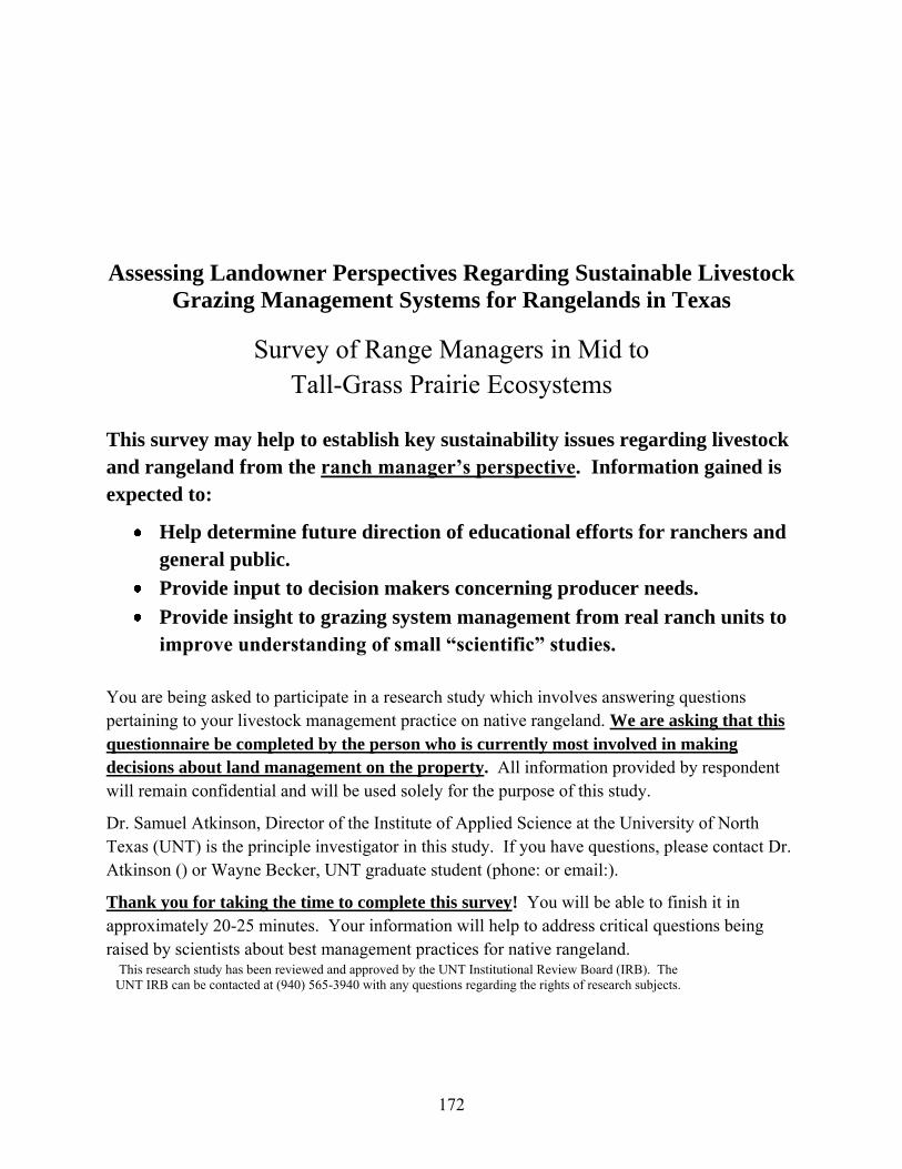
Assessing Landowner Perspectives Regarding Sustainable Livestock
Grazing Management Systems for Rangelands in Texas
Survey of Range Managers in Mid to Tall-Grass Prairie Ecosystems
This survey may help to establish key sustainability issues regarding livestock
and rangeland from the ranch manager’s perspective. Information gained is
expected to:
Help determine future direction of educational efforts for ranchers and
general public.
Provide input to decision makers concerning producer needs.
Provide insight to grazing system management from real ranch units to
improve understanding of small “scientific” studies.
You are being asked to participate in a research study which involves answering questions pertaining to your livestock management practice on native rangeland. We are asking that this
questionnaire be completed by the person who is currently most involved in making
decisions about land management on the property. All information provided by respondent will remain confidential and will be used solely for the purpose of this study.
Dr. Samuel Atkinson, Director of the Institute of Applied Science at the University of North Texas (UNT) is the principle investigator in this study. If you have questions, please contact Dr. Atkinson () or Wayne Becker, UNT graduate student (phone: or email:).
Thank you for taking the time to complete this survey! You will be able to finish it in approximately 20-25 minutes. Your information will help to address critical questions being raised by scientists about best management practices for native rangeland.
This research study has been reviewed and approved by the UNT Institutional Review Board (IRB). The UNT IRB can be contacted at (940) 565-3940 with any questions regarding the rights of research subjects.
172
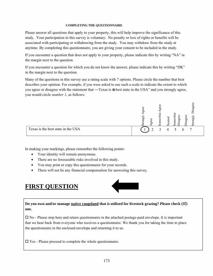
COMPLETING THE QUESTIONNAIRE
Please answer all questions that apply to your property, this will help improve the significance of this study. Your participation in this survey is voluntary. No penalty or loss of rights or benefits will be associated with participating or withdrawing from the study. You may withdraw from the study at anytime. By completing this questionnaire, you are giving your consent to be included in the study.
If you encounter a question that does not apply to your property, please indicate this by writing ―NA‖ in
the margin next to the question.
If you encounter a question for which you do not know the answer, please indicate this by writing ―DK‖ in the margin next to the question.
Many of the questions in this survey use a rating scale with 7 options. Please circle the number that best describes your opinion. For example, if you were asked to use such a scale to indicate the extent to which you agree or disagree with the statement that ―Texas is the best state in the USA‖ and you strongly agree, you would circle number 1, as follows:
Texas is the best state in the USA 1 2 3 4 5 6 7
In making your markings, please remember the following points: Your identity will remain anonymous. There are no foreseeable risks involved in this study. You may print or copy this questionnaire for your records. There will not be any financial compensation for answering this survey.
FIRST QUESTION
Do you own and/or manage native rangeland that is utilized for livestock grazing? Please check ()
one.
No - Please stop here and return questionnaire in the attached postage-paid envelope. It is important that we hear back from everyone who receives a questionnaire. We thank you for taking the time to place the questionnaire in the enclosed envelope and returning it to us.
Yes - Please proceed to complete the whole questionnaire.
Stro
ngly
Agr
ee
Agr
ee
Som
ewha
t Agr
ee
Neu
tral
Som
ewha
t D
isag
ree
Dis
agre
e
Stro
ngly
Dis
agre
e
173
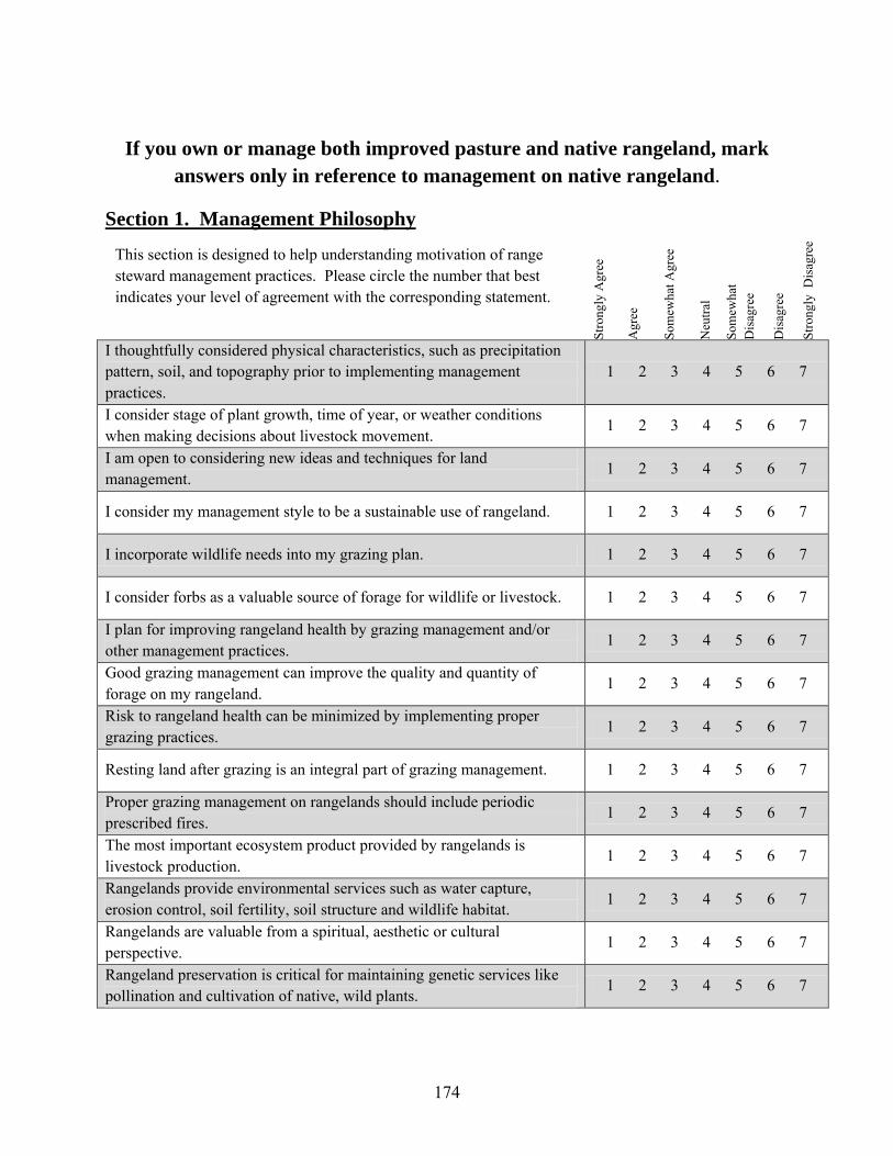
If you own or manage both improved pasture and native rangeland, mark
answers only in reference to management on native rangeland.
Section 1. Management Philosophy
I thoughtfully considered physical characteristics, such as precipitation pattern, soil, and topography prior to implementing management practices.
1 2 3 4 5 6 7
I consider stage of plant growth, time of year, or weather conditions when making decisions about livestock movement.
1 2 3 4 5 6 7
I am open to considering new ideas and techniques for land management.
1 2 3 4 5 6 7
I consider my management style to be a sustainable use of rangeland. 1 2 3 4 5 6 7
I incorporate wildlife needs into my grazing plan. 1 2 3 4 5 6 7
I consider forbs as a valuable source of forage for wildlife or livestock. 1 2 3 4 5 6 7
I plan for improving rangeland health by grazing management and/or other management practices.
1 2 3 4 5 6 7
Good grazing management can improve the quality and quantity of forage on my rangeland.
1 2 3 4 5 6 7
Risk to rangeland health can be minimized by implementing proper grazing practices.
1 2 3 4 5 6 7
Resting land after grazing is an integral part of grazing management. 1 2 3 4 5 6 7
Proper grazing management on rangelands should include periodic prescribed fires.
1 2 3 4 5 6 7
The most important ecosystem product provided by rangelands is livestock production.
1 2 3 4 5 6 7
Rangelands provide environmental services such as water capture, erosion control, soil fertility, soil structure and wildlife habitat.
1 2 3 4 5 6 7
Rangelands are valuable from a spiritual, aesthetic or cultural perspective.
1 2 3 4 5 6 7
Rangeland preservation is critical for maintaining genetic services like pollination and cultivation of native, wild plants.
1 2 3 4 5 6 7
Stro
ngly
Agr
ee
Agr
ee
Som
ewha
t Agr
ee
Neu
tral
Som
ewha
t D
isag
ree
Dis
agre
e
Stro
ngly
Dis
agre
e
This section is designed to help understanding motivation of range steward management practices. Please circle the number that best indicates your level of agreement with the corresponding statement.
174
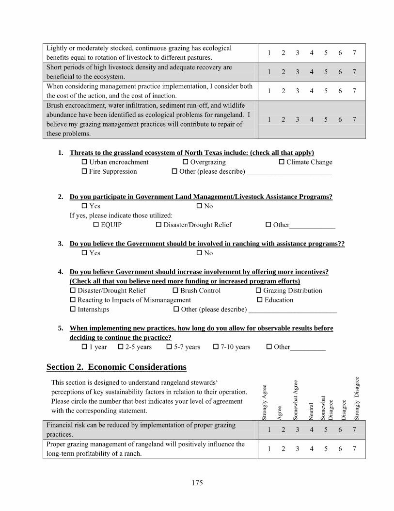
Lightly or moderately stocked, continuous grazing has ecological benefits equal to rotation of livestock to different pastures.
1 2 3 4 5 6 7
Short periods of high livestock density and adequate recovery are beneficial to the ecosystem.
1 2 3 4 5 6 7
When considering management practice implementation, I consider both the cost of the action, and the cost of inaction.
1 2 3 4 5 6 7
Brush encroachment, water infiltration, sediment run-off, and wildlife abundance have been identified as ecological problems for rangeland. I believe my grazing management practices will contribute to repair of these problems.
1 2 3 4 5 6 7
1. Threats to the grassland ecosystem of North Texas include: (check all that apply)
Urban encroachment Overgrazing Climate Change Fire Suppression Other (please describe) ________________________
2. Do you participate in Government Land Management/Livestock Assistance Programs?
Yes No If yes, please indicate those utilized:
EQUIP Disaster/Drought Relief Other_____________
3. Do you believe the Government should be involved in ranching with assistance programs??
Yes No
4. Do you believe Government should increase involvement by offering more incentives?
(Check all that you believe need more funding or increased program efforts)
Disaster/Drought Relief Brush Control Grazing Distribution Reacting to Impacts of Mismanagement Education Internships Other (please describe) _________________________
5. When implementing new practices, how long do you allow for observable results before
deciding to continue the practice?
1 year 2-5 years 5-7 years 7-10 years Other__________
Section 2. Economic Considerations
Financial risk can be reduced by implementation of proper grazing practices.
1 2 3 4 5 6 7
Proper grazing management of rangeland will positively influence the long-term profitability of a ranch.
1 2 3 4 5 6 7
Stro
ngly
Agr
ee
Agr
ee
Som
ewha
t Agr
ee
Neu
tral
Som
ewha
t D
isag
ree
Dis
agre
e
Stro
ngly
Dis
agre
e
This section is designed to understand rangeland stewards‘ perceptions of key sustainability factors in relation to their operation. Please circle the number that best indicates your level of agreement with the corresponding statement.
175
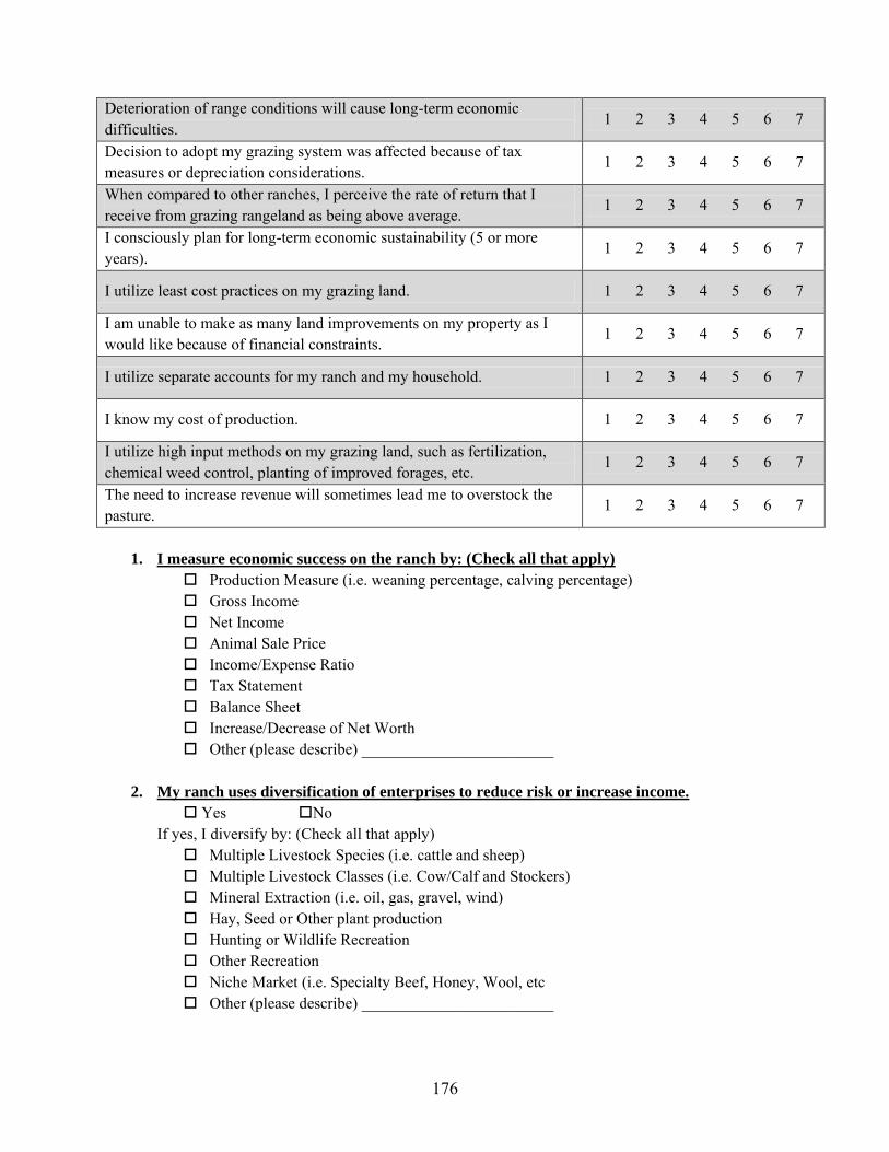
Deterioration of range conditions will cause long-term economic difficulties.
1 2 3 4 5 6 7
Decision to adopt my grazing system was affected because of tax measures or depreciation considerations.
1 2 3 4 5 6 7
When compared to other ranches, I perceive the rate of return that I receive from grazing rangeland as being above average.
1 2 3 4 5 6 7
I consciously plan for long-term economic sustainability (5 or more years).
1 2 3 4 5 6 7
I utilize least cost practices on my grazing land. 1 2 3 4 5 6 7
I am unable to make as many land improvements on my property as I would like because of financial constraints.
1 2 3 4 5 6 7
I utilize separate accounts for my ranch and my household. 1 2 3 4 5 6 7
I know my cost of production. 1 2 3 4 5 6 7
I utilize high input methods on my grazing land, such as fertilization, chemical weed control, planting of improved forages, etc.
1 2 3 4 5 6 7
The need to increase revenue will sometimes lead me to overstock the pasture.
1 2 3 4 5 6 7
1. I measure economic success on the ranch by: (Check all that apply)
Production Measure (i.e. weaning percentage, calving percentage) Gross Income Net Income Animal Sale Price Income/Expense Ratio Tax Statement Balance Sheet Increase/Decrease of Net Worth Other (please describe) ________________________
2. My ranch uses diversification of enterprises to reduce risk or increase income.
Yes No If yes, I diversify by: (Check all that apply)
Multiple Livestock Species (i.e. cattle and sheep) Multiple Livestock Classes (i.e. Cow/Calf and Stockers) Mineral Extraction (i.e. oil, gas, gravel, wind) Hay, Seed or Other plant production Hunting or Wildlife Recreation Other Recreation Niche Market (i.e. Specialty Beef, Honey, Wool, etc Other (please describe) ________________________
176
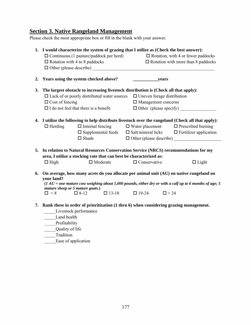
Section 3. Native Rangeland Management Please check the most appropriate box or fill in the blank with your answer.
1. I would characterize the system of grazing that I utilize as (Check the best answer):
Continuous (1 pasture/paddock per herd) Rotation, with 4 or fewer paddocks Rotation with 4 to 8 paddocks Rotation with more than 8 paddocks Other (please describe) ______________________________________________________
2. Years using the system checked above? ___________years
3. The largest obstacle to increasing livestock distribution is (Check all that apply):
Lack of or poorly distributed water sources Uneven forage distribution Cost of fencing Management concerns I do not feel that there is a benefit Other (please specify) ________________
4. I utilize the following to help distribute livestock over the rangeland (Check all that apply):
Herding Internal fencing Water placement Prescribed burning Supplemental feeds Salt/mineral licks Fertilizer application Shade Other (please describe) _____________________
5. In relation to Natural Resources Conservation Service (NRCS) recommendations for my
area, I utilize a stocking rate that can best be characterized as:
High Moderate Conservative Light
6. On average, how many acres do you allocate per animal unit (AU) on native rangeland on
your land? (1 AU = one mature cow weighing about 1,000 pounds, either dry or with a calf up to 6 months of age; 5
mature sheep or 5 mature goats.)
< 8 8-12 13-18 19-24 > 24
7. Rank these in order of prioritization (1 thru 6) when considering grazing management.
_____Livestock performance _____Land health _____Profitability _____Quality of life _____Tradition _____Ease of application
177
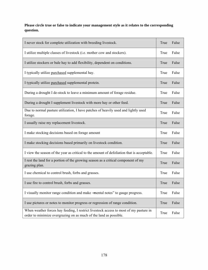
Please circle true or false to indicate your management style as it relates to the corresponding
question.
I never stock for complete utilization with breeding livestock. True False
I utilize multiple classes of livestock (i.e. mother cow and stockers). True False
I utilize stockers or bale hay to add flexibility, dependent on conditions. True False
I typically utilize purchased supplemental hay. True False
I typically utilize purchased supplemental protein. True False
During a drought I de-stock to leave a minimum amount of forage residue. True False
During a drought I supplement livestock with more hay or other feed. True False
Due to normal pasture utilization, I have patches of heavily used and lightly used forage.
True False
I usually raise my replacement livestock. True False
I make stocking decisions based on forage amount True False
I make stocking decisions based primarily on livestock condition. True False
I view the season of the year as critical to the amount of defoliation that is acceptable. True False
I rest the land for a portion of the growing season as a critical component of my grazing plan.
True False
I use chemical to control brush, forbs and grasses. True False
I use fire to control brush, forbs and grasses. True False
I visually monitor range condition and make ―mental notes‖ to gauge progress. True False
I use pictures or notes to monitor progress or regression of range condition. True False
When weather forces hay feeding, I restrict livestock access to most of my pasture in order to minimize overgrazing on as much of the land as possible.
True False
178
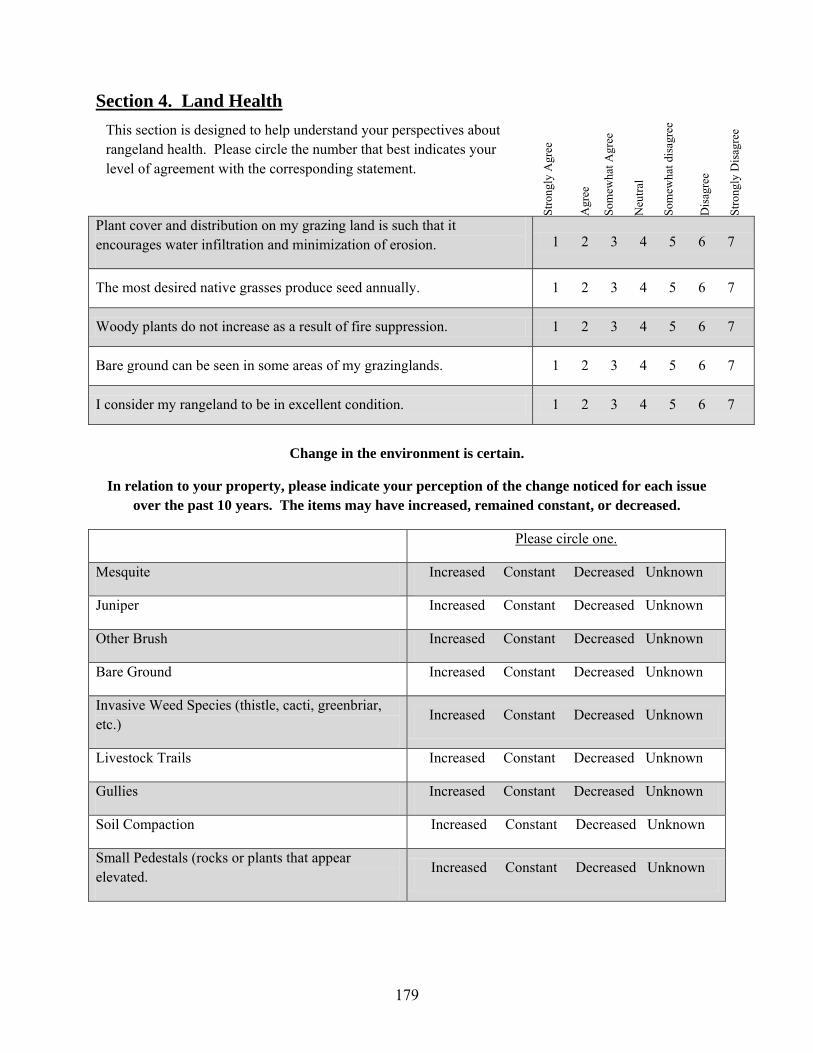
Section 4. Land Health
Plant cover and distribution on my grazing land is such that it encourages water infiltration and minimization of erosion. 1 2 3 4 5 6 7
The most desired native grasses produce seed annually. 1 2 3 4 5 6 7
Woody plants do not increase as a result of fire suppression. 1 2 3 4 5 6 7
Bare ground can be seen in some areas of my grazinglands. 1 2 3 4 5 6 7
I consider my rangeland to be in excellent condition. 1 2 3 4 5 6 7
Change in the environment is certain.
In relation to your property, please indicate your perception of the change noticed for each issue
over the past 10 years. The items may have increased, remained constant, or decreased.
Please circle one.
Mesquite Increased Constant Decreased Unknown
Juniper Increased Constant Decreased Unknown
Other Brush Increased Constant Decreased Unknown
Bare Ground Increased Constant Decreased Unknown
Invasive Weed Species (thistle, cacti, greenbriar, etc.)
Increased Constant Decreased Unknown
Livestock Trails Increased Constant Decreased Unknown
Gullies Increased Constant Decreased Unknown
Soil Compaction Increased Constant Decreased Unknown
Small Pedestals (rocks or plants that appear elevated.
Increased Constant Decreased Unknown
Stro
ngly
Agr
ee
Agr
ee
Som
ewha
t Agr
ee
Neu
tral
Som
ewha
t dis
agre
e
Dis
agre
e
Stro
ngly
Dis
agre
e This section is designed to help understand your perspectives about rangeland health. Please circle the number that best indicates your level of agreement with the corresponding statement.
179
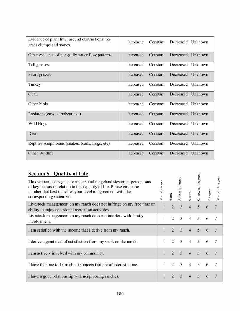
Evidence of plant litter around obstructions like grass clumps and stones.
Increased Constant Decreased Unknown
Other evidence of non-gully water flow patterns. Increased Constant Decreased Unknown
Tall grasses Increased Constant Decreased Unknown
Short grasses Increased Constant Decreased Unknown
Turkey Increased Constant Decreased Unknown
Quail Increased Constant Decreased Unknown
Other birds Increased Constant Decreased Unknown
Predators (coyote, bobcat etc.) Increased Constant Decreased Unknown
Wild Hogs Increased Constant Decreased Unknown
Deer Increased Constant Decreased Unknown
Reptiles/Amphibians (snakes, toads, frogs, etc) Increased Constant Decreased Unknown
Other Wildlife Increased Constant Decreased Unknown
Section 5. Quality of Life
This section is designed to understand rangeland stewards‘ perceptions of key factors in relation to their quality of life. Please circle the number that best indicates your level of agreement with the corresponding statement.
Livestock management on my ranch does not infringe on my free time or ability to enjoy occasional recreation activities.
1 2 3 4 5 6 7
Livestock management on my ranch does not interfere with family involvement.
1 2 3 4 5 6 7
I am satisfied with the income that I derive from my ranch. 1 2 3 4 5 6 7
I derive a great deal of satisfaction from my work on the ranch. 1 2 3 4 5 6 7
I am actively involved with my community. 1 2 3 4 5 6 7
I have the time to learn about subjects that are of interest to me. 1 2 3 4 5 6 7
I have a good relationship with neighboring ranches. 1 2 3 4 5 6 7
Stro
ngly
Agr
ee
Agr
ee
Som
ewha
t Agr
ee
Neu
tral
Som
ewha
t dis
agre
e
Dis
agre
e
Stro
ngly
Dis
agre
e
180
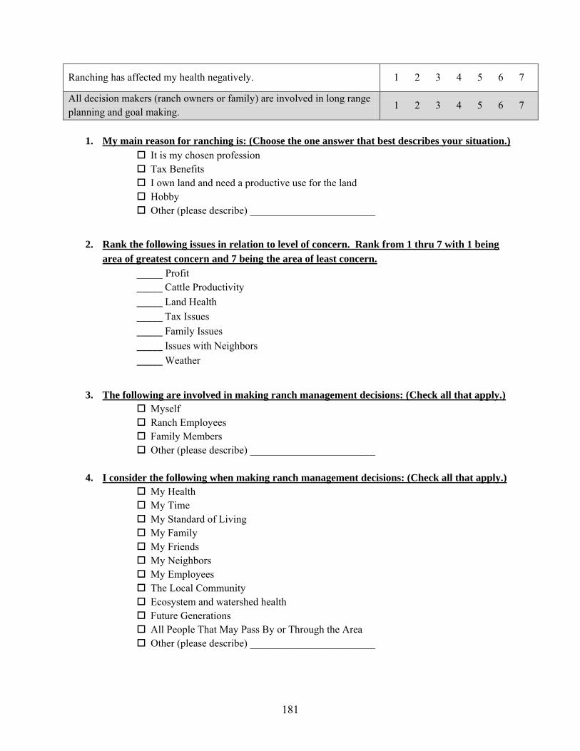
Ranching has affected my health negatively. 1 2 3 4 5 6 7
All decision makers (ranch owners or family) are involved in long range planning and goal making.
1 2 3 4 5 6 7
1. My main reason for ranching is: (Choose the one answer that best describes your situation.)
It is my chosen profession Tax Benefits I own land and need a productive use for the land Hobby Other (please describe) ________________________
2. Rank the following issues in relation to level of concern. Rank from 1 thru 7 with 1 being
area of greatest concern and 7 being the area of least concern.
_____ Profit _____ Cattle Productivity _____ Land Health _____ Tax Issues _____ Family Issues _____ Issues with Neighbors _____ Weather
3. The following are involved in making ranch management decisions: (Check all that apply.)
Myself Ranch Employees Family Members Other (please describe) ________________________
4. I consider the following when making ranch management decisions: (Check all that apply.)
My Health My Time My Standard of Living My Family My Friends My Neighbors My Employees The Local Community Ecosystem and watershed health Future Generations All People That May Pass By or Through the Area Other (please describe) ________________________
181
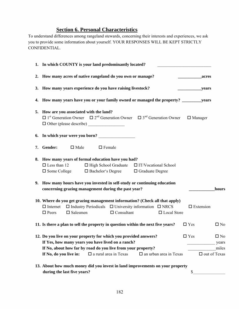
Section 6. Personal Characteristics To understand differences among rangeland stewards, concerning their interests and experiences, we ask you to provide some information about yourself. YOUR RESPONSES WILL BE KEPT STRICTLY CONFIDENTIAL.
1. In which COUNTY is your land predominantly located? _________________________ 2. How many acres of native rangeland do you own or manage? ___________acres 3. How many years experience do you have raising livestock? ___________years
4. How many years have you or your family owned or managed the property? _________years
5. How are you associated with the land?
1st Generation Owner 2nd Generation Owner 3nd Generation Owner Manager Other (please describe) _________________
6. In which year were you born? _________________
7. Gender: Male Female
8. How many years of formal education have you had?
Less than 12 High School Graduate IT/Vocational School Some College Bachelor‘s Degree Graduate Degree
9. How many hours have you invested in self-study or continuing education
concerning grazing management during the past year? ____________hours
10. Where do you get grazing management information? (Check all that apply)
Internet Industry Periodicals University information NRCS Extension Peers Salesmen Consultant Local Store
11. Is there a plan to sell the property in question within the next five years? Yes No
12. Do you live on your property for which you provided answers? Yes No
If Yes, how many years you have lived on a ranch? _____________ years
If No, about how far by road do you live from your property? _____________miles If No, do you live in: a rural area in Texas an urban area in Texas out of Texas
13. About how much money did you invest in land improvements on your property during the last five years? $_______________
182
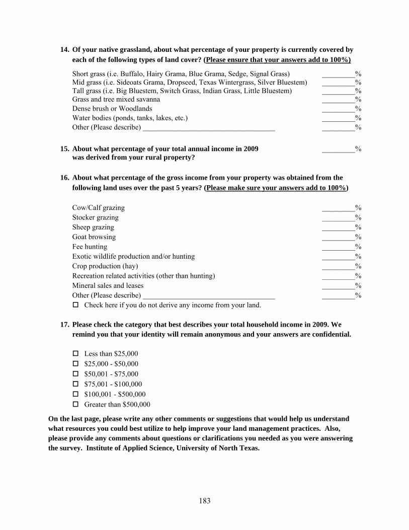
14. Of your native grassland, about what percentage of your property is currently covered by
each of the following types of land cover? (Please ensure that your answers add to 100%)
Short grass (i.e. Buffalo, Hairy Grama, Blue Grama, Sedge, Signal Grass) _________% Mid grass (i.e. Sideoats Grama, Dropseed, Texas Wintergrass, Silver Bluestem) _________% Tall grass (i.e. Big Bluestem, Switch Grass, Indian Grass, Little Bluestem) _________% Grass and tree mixed savanna _________% Dense brush or Woodlands _________% Water bodies (ponds, tanks, lakes, etc.) _________% Other (Please describe) ____________________________________ _________%
15. About what percentage of your total annual income in 2009 _________%
was derived from your rural property?
16. About what percentage of the gross income from your property was obtained from the
following land uses over the past 5 years? (Please make sure your answers add to 100%)
Cow/Calf grazing _________% Stocker grazing _________% Sheep grazing _________% Goat browsing _________% Fee hunting _________% Exotic wildlife production and/or hunting _________% Crop production (hay) _________% Recreation related activities (other than hunting) _________% Mineral sales and leases _________% Other (Please describe) ____________________________________ _________% Check here if you do not derive any income from your land.
17. Please check the category that best describes your total household income in 2009. We
remind you that your identity will remain anonymous and your answers are confidential.
Less than $25,000 $25,000 - $50,000 $50,001 - $75,000 $75,001 - $100,000 $100,001 - $500,000 Greater than $500,000
On the last page, please write any other comments or suggestions that would help us understand
what resources you could best utilize to help improve your land management practices. Also,
please provide any comments about questions or clarifications you needed as you were answering
the survey. Institute of Applied Science, University of North Texas.
183

Your participation is greatly appreciated. Please send the questionnaire back to us in the enclosed postage-paid envelope. Feel free to offer any addition comments or
thoughts on native range grazing management that you may have.
Thank You!
Optional:
Name: __________________________________________
Address: ________________________________________
City, State, Zip: __________________________________
Email: __________________________________________
184

APPENDIX B
NON-RESPONSE BIAS QUESTIONNAIRE
185
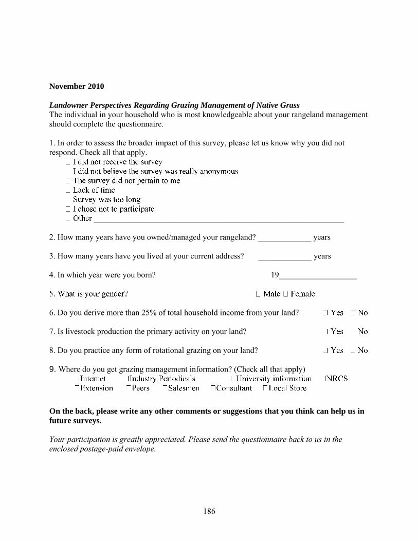
November 2010
Landowner Perspectives Regarding Grazing Management of Native Grass
The individual in your household who is most knowledgeable about your rangeland management should complete the questionnaire. 1. In order to assess the broader impact of this survey, please let us know why you did not respond. Check all that apply.
r _____________________________________________________________ 2. How many years have you owned/managed your rangeland? _____________ years 3. How many years have you lived at your current address? _____________ years 4. In which year were you born? 19___________________
6. Do you derive more than 25% of total household income from your land? 7. Is livestock production the primary activity on your land? 8. Do you practice any form of rotational grazing on your land? 9. Where do you get grazing management information? (Check all that apply)
On the back, please write any other comments or suggestions that you think can help us in
future surveys.
Your participation is greatly appreciated. Please send the questionnaire back to us in the enclosed postage-paid envelope.
186
APPENDIX C
DESCRIPTIVE STATISTICS
187
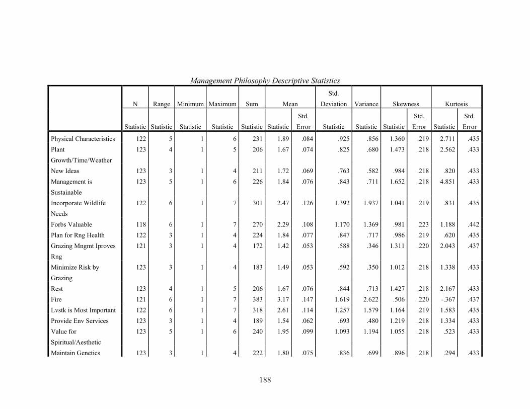
Management Philosophy Descriptive Statistics
N Range Minimum Maximum Sum Mean
Std. Deviation Variance Skewness Kurtosis
Statistic Statistic Statistic Statistic Statistic Statistic Std.
Error Statistic Statistic Statistic Std.
Error Statistic Std.
Error
Physical Characteristics 122 5 1 6 231 1.89 .084 .925 .856 1.360 .219 2.711 .435 Plant Growth/Time/Weather
123 4 1 5 206 1.67 .074 .825 .680 1.473 .218 2.562 .433
New Ideas 123 3 1 4 211 1.72 .069 .763 .582 .984 .218 .820 .433 Management is Sustainable
123 5 1 6 226 1.84 .076 .843 .711 1.652 .218 4.851 .433
Incorporate Wildlife Needs
122 6 1 7 301 2.47 .126 1.392 1.937 1.041 .219 .831 .435
Forbs Valuable 118 6 1 7 270 2.29 .108 1.170 1.369 .981 .223 1.188 .442 Plan for Rng Health 122 3 1 4 224 1.84 .077 .847 .717 .986 .219 .620 .435 Grazing Mngmt Iproves Rng
121 3 1 4 172 1.42 .053 .588 .346 1.311 .220 2.043 .437
Minimize Risk by Grazing
123 3 1 4 183 1.49 .053 .592 .350 1.012 .218 1.338 .433
Rest 123 4 1 5 206 1.67 .076 .844 .713 1.427 .218 2.167 .433 Fire 121 6 1 7 383 3.17 .147 1.619 2.622 .506 .220 -.367 .437 Lvstk is Most Important 122 6 1 7 318 2.61 .114 1.257 1.579 1.164 .219 1.583 .435 Provide Env Services 123 3 1 4 189 1.54 .062 .693 .480 1.219 .218 1.334 .433 Value for Spiritual/Aesthetic
123 5 1 6 240 1.95 .099 1.093 1.194 1.055 .218 .523 .433
Maintain Genetics 123 3 1 4 222 1.80 .075 .836 .699 .896 .218 .294 .433
188
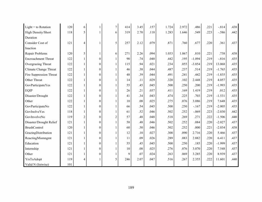
Light = to Rotation 120 6 1 7 414 3.45 .157 1.724 2.972 .486 .221 -.814 .438 High Density/Short Duration
118 5 1 6 319 2.70 .118 1.283 1.646 .549 .223 -.586 .442
Consider Cost of Inaction
121 4 1 5 257 2.12 .079 .871 .760 .677 .220 .361 .437
Repair Problems 120 5 1 6 271 2.26 .094 1.033 1.067 .810 .221 .738 .438 Encroachment Threat 122 1 0 1 90 .74 .040 .442 .195 -1.094 .219 -.816 .435 Overgrazing Threat 122 1 0 1 115 .94 .021 .234 .055 -3.854 .219 13.068 .435 Climate Change Threat 122 1 0 1 46 .38 .044 .487 .237 .514 .219 -1.765 .435 Fire Suppression Threat 122 1 0 1 48 .39 .044 .491 .241 .442 .219 -1.835 .435 Other Threat 122 1 0 1 14 .11 .029 .320 .102 2.448 .219 4.057 .435 GovParticipateYes 122 1 0 1 55 .45 .045 .500 .250 .200 .219 -1.993 .435 EQIP 122 1 0 1 26 .21 .037 .411 .169 1.419 .219 .012 .435 Disaster/Drought 122 1 0 1 41 .34 .043 .474 .225 .703 .219 -1.531 .435 Other 122 1 0 1 10 .08 .025 .275 .076 3.086 .219 7.648 .435 GovParticipateNo 122 1 0 1 66 .54 .045 .500 .250 -.167 .219 -2.005 .435 GovInolveYes 118 1 0 1 61 .52 .046 .502 .252 -.069 .223 -2.030 .442 GovInvolveNo 119 2 0 2 57 .48 .048 .518 .269 .271 .222 -1.506 .440 Disaster/Drought Relief 121 1 0 1 58 .48 .046 .502 .252 .084 .220 -2.027 .437 BrushControl 120 1 0 1 60 .50 .046 .502 .252 .000 .221 -2.034 .438 GrazingDistribution 121 1 0 1 12 .10 .027 .300 .090 2.716 .220 5.466 .437 ReactingMismngmt 121 1 0 1 11 .09 .026 .289 .083 2.882 .220 6.411 .437 Education 121 1 0 1 55 .45 .045 .500 .250 .185 .220 -1.999 .437 Internship 121 1 0 1 10 .08 .025 .276 .076 3.070 .220 7.548 .437 Other 121 1 0 1 9 .07 .024 .263 .069 3.285 .220 8.939 .437 YrsToAdopt 119 4 1 5 246 2.07 .047 .516 .267 2.355 .222 11.601 .440 Valid N (listwise) 101
189
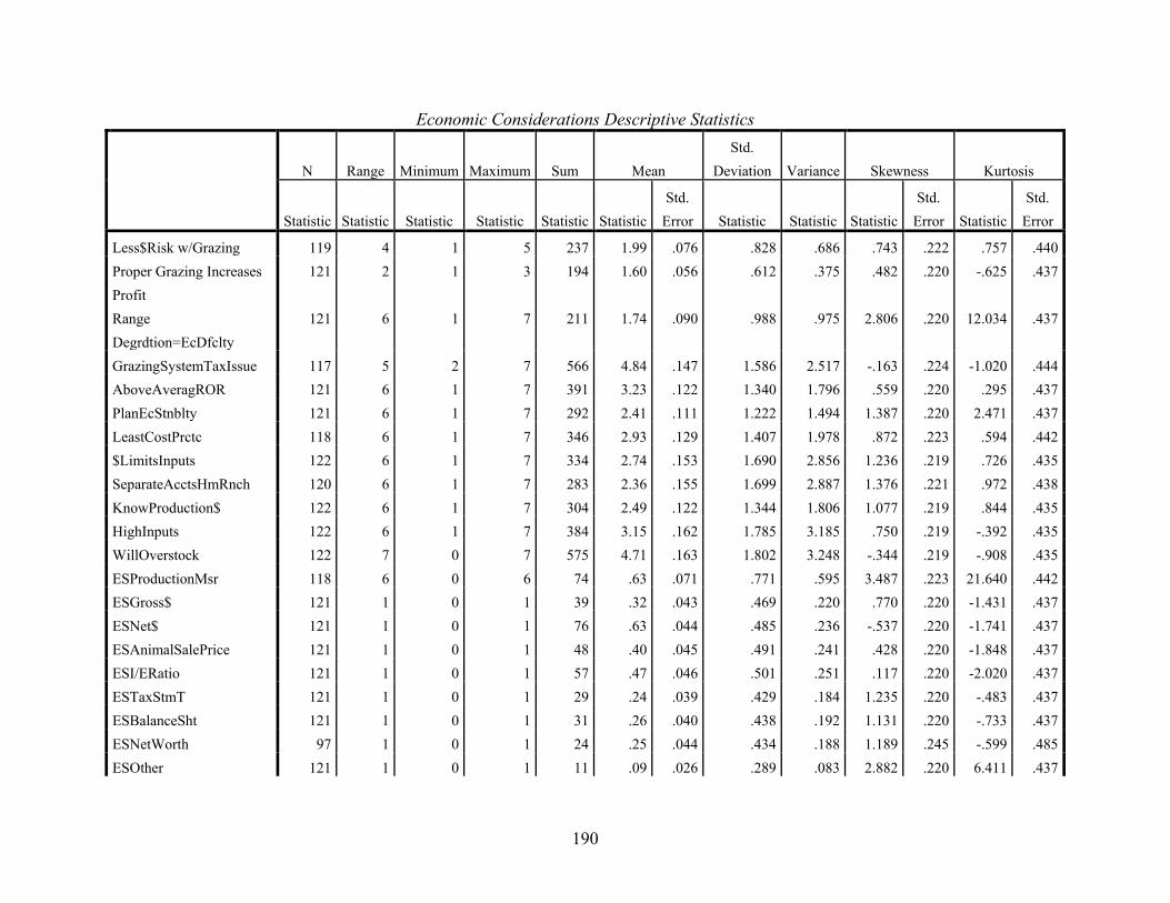
Economic Considerations Descriptive Statistics
N Range Minimum Maximum Sum Mean
Std. Deviation Variance Skewness Kurtosis
Statistic Statistic Statistic Statistic Statistic Statistic Std.
Error Statistic Statistic Statistic Std.
Error Statistic Std.
Error
Less$Risk w/Grazing 119 4 1 5 237 1.99 .076 .828 .686 .743 .222 .757 .440 Proper Grazing Increases Profit
121 2 1 3 194 1.60 .056 .612 .375 .482 .220 -.625 .437
Range Degrdtion=EcDfclty
121 6 1 7 211 1.74 .090 .988 .975 2.806 .220 12.034 .437
GrazingSystemTaxIssue 117 5 2 7 566 4.84 .147 1.586 2.517 -.163 .224 -1.020 .444 AboveAveragROR 121 6 1 7 391 3.23 .122 1.340 1.796 .559 .220 .295 .437 PlanEcStnblty 121 6 1 7 292 2.41 .111 1.222 1.494 1.387 .220 2.471 .437 LeastCostPrctc 118 6 1 7 346 2.93 .129 1.407 1.978 .872 .223 .594 .442 $LimitsInputs 122 6 1 7 334 2.74 .153 1.690 2.856 1.236 .219 .726 .435 SeparateAcctsHmRnch 120 6 1 7 283 2.36 .155 1.699 2.887 1.376 .221 .972 .438 KnowProduction$ 122 6 1 7 304 2.49 .122 1.344 1.806 1.077 .219 .844 .435 HighInputs 122 6 1 7 384 3.15 .162 1.785 3.185 .750 .219 -.392 .435 WillOverstock 122 7 0 7 575 4.71 .163 1.802 3.248 -.344 .219 -.908 .435 ESProductionMsr 118 6 0 6 74 .63 .071 .771 .595 3.487 .223 21.640 .442 ESGross$ 121 1 0 1 39 .32 .043 .469 .220 .770 .220 -1.431 .437 ESNet$ 121 1 0 1 76 .63 .044 .485 .236 -.537 .220 -1.741 .437 ESAnimalSalePrice 121 1 0 1 48 .40 .045 .491 .241 .428 .220 -1.848 .437 ESI/ERatio 121 1 0 1 57 .47 .046 .501 .251 .117 .220 -2.020 .437 ESTaxStmT 121 1 0 1 29 .24 .039 .429 .184 1.235 .220 -.483 .437 ESBalanceSht 121 1 0 1 31 .26 .040 .438 .192 1.131 .220 -.733 .437 ESNetWorth 97 1 0 1 24 .25 .044 .434 .188 1.189 .245 -.599 .485 ESOther 121 1 0 1 11 .09 .026 .289 .083 2.882 .220 6.411 .437
190
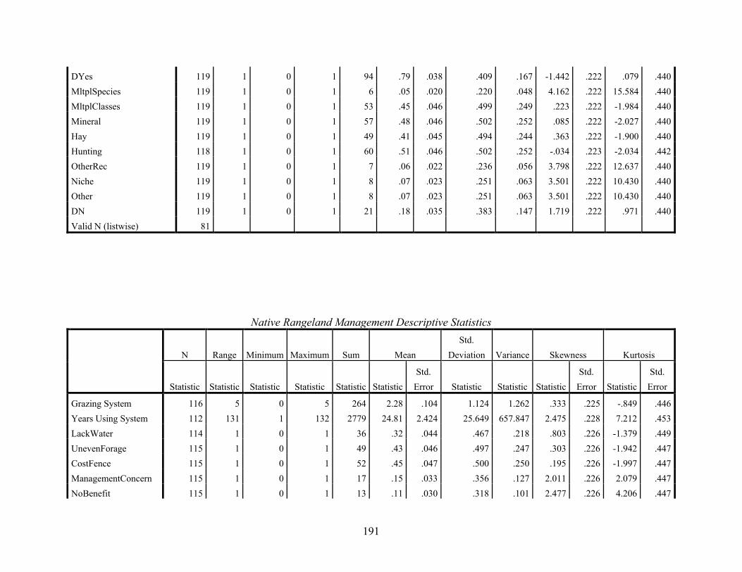
DYes 119 1 0 1 94 .79 .038 .409 .167 -1.442 .222 .079 .440 MltplSpecies 119 1 0 1 6 .05 .020 .220 .048 4.162 .222 15.584 .440 MltplClasses 119 1 0 1 53 .45 .046 .499 .249 .223 .222 -1.984 .440 Mineral 119 1 0 1 57 .48 .046 .502 .252 .085 .222 -2.027 .440 Hay 119 1 0 1 49 .41 .045 .494 .244 .363 .222 -1.900 .440 Hunting 118 1 0 1 60 .51 .046 .502 .252 -.034 .223 -2.034 .442 OtherRec 119 1 0 1 7 .06 .022 .236 .056 3.798 .222 12.637 .440 Niche 119 1 0 1 8 .07 .023 .251 .063 3.501 .222 10.430 .440 Other 119 1 0 1 8 .07 .023 .251 .063 3.501 .222 10.430 .440 DN 119 1 0 1 21 .18 .035 .383 .147 1.719 .222 .971 .440 Valid N (listwise) 81
Native Rangeland Management Descriptive Statistics
N Range Minimum Maximum Sum Mean
Std. Deviation Variance Skewness Kurtosis
Statistic Statistic Statistic Statistic Statistic Statistic Std.
Error Statistic Statistic Statistic Std.
Error Statistic Std.
Error
Grazing System 116 5 0 5 264 2.28 .104 1.124 1.262 .333 .225 -.849 .446 Years Using System 112 131 1 132 2779 24.81 2.424 25.649 657.847 2.475 .228 7.212 .453 LackWater 114 1 0 1 36 .32 .044 .467 .218 .803 .226 -1.379 .449 UnevenForage 115 1 0 1 49 .43 .046 .497 .247 .303 .226 -1.942 .447 CostFence 115 1 0 1 52 .45 .047 .500 .250 .195 .226 -1.997 .447 ManagementConcern 115 1 0 1 17 .15 .033 .356 .127 2.011 .226 2.079 .447 NoBenefit 115 1 0 1 13 .11 .030 .318 .101 2.477 .226 4.206 .447
191
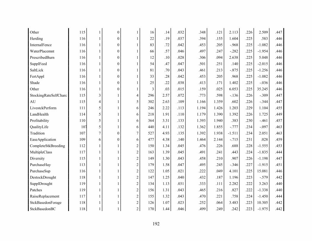
Other 115 1 0 1 16 .14 .032 .348 .121 2.113 .226 2.509 .447 Herding 116 1 0 1 22 .19 .037 .394 .155 1.604 .225 .583 .446 InternalFence 116 1 0 1 83 .72 .042 .453 .205 -.968 .225 -1.082 .446 WaterPlacemnt 116 1 0 1 66 .57 .046 .497 .247 -.282 .225 -1.954 .446 PrescribedBurn 116 1 0 1 12 .10 .028 .306 .094 2.638 .225 5.048 .446 SupplFeed 116 1 0 1 54 .47 .047 .501 .251 .140 .225 -2.015 .446 SaltLick 116 1 0 1 81 .70 .043 .461 .213 -.875 .225 -1.256 .446 FertAppl 116 1 0 1 33 .28 .042 .453 .205 .968 .225 -1.082 .446 Shade 116 1 0 1 25 .22 .038 .413 .171 1.402 .225 -.036 .446 Other 116 1 0 1 3 .03 .015 .159 .025 6.053 .225 35.245 .446 StockingRateSelfCharc 115 3 1 4 296 2.57 .072 .773 .598 -.136 .226 -.309 .447 AU 115 4 1 5 302 2.63 .109 1.166 1.359 .602 .226 -.344 .447 LivestckPerform 111 5 1 6 246 2.22 .113 1.194 1.426 1.203 .229 1.104 .455 LandHealth 114 5 1 6 218 1.91 .110 1.179 1.390 1.392 .226 1.725 .449 Profitability 110 5 1 6 364 3.31 .133 1.393 1.940 .383 .230 -.461 .457 QualityLife 107 5 1 6 440 4.11 .132 1.362 1.855 -.777 .234 -.097 .463 Tradition 107 7 0 7 527 4.93 .135 1.392 1.938 -1.511 .234 2.051 .463 EaseApplication 109 6 0 6 477 4.38 .140 1.464 2.144 -.715 .231 .028 .459 CompleteStkBreeding 112 1 1 2 150 1.34 .045 .476 .226 .688 .228 -1.555 .453 MultipleClass 117 1 1 2 163 1.39 .045 .491 .241 .443 .224 -1.835 .444 Diversity 115 1 1 2 149 1.30 .043 .458 .210 .907 .226 -1.198 .447 PurchaseHay 113 1 1 2 179 1.58 .047 .495 .245 -.346 .227 -1.915 .451 PurchaseSup 116 1 1 2 122 1.05 .021 .222 .049 4.101 .225 15.081 .446 DestockDrought 118 1 1 2 147 1.25 .040 .432 .187 1.196 .223 -.579 .442 SupplDrought 119 1 1 2 134 1.13 .031 .333 .111 2.282 .222 3.263 .440 Patches 119 1 1 2 156 1.31 .043 .465 .216 .827 .222 -1.338 .440 RaiseReplacement 117 1 1 2 155 1.32 .043 .470 .221 .758 .224 -1.450 .444 StckBasedonForage 118 1 1 2 126 1.07 .023 .252 .064 3.483 .223 10.305 .442 StckBasedonBC 118 1 1 2 170 1.44 .046 .499 .249 .242 .223 -1.975 .442
192
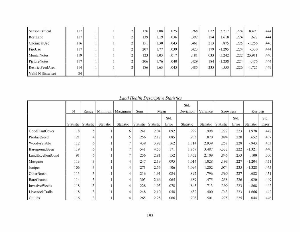
SeasonCritical 117 1 1 2 126 1.08 .025 .268 .072 3.217 .224 8.493 .444 RestLand 117 1 1 2 139 1.19 .036 .392 .154 1.618 .224 .627 .444 ChemicalUse 116 1 1 2 151 1.30 .043 .461 .213 .875 .225 -1.256 .446 FireUse 117 1 1 2 207 1.77 .039 .423 .179 -1.295 .224 -.330 .444 MentalNotes 119 1 1 2 123 1.03 .017 .181 .033 5.242 .222 25.911 .440 PictureNotes 117 1 1 2 206 1.76 .040 .429 .184 -1.238 .224 -.476 .444 RestrictFeedArea 114 1 1 2 186 1.63 .045 .485 .235 -.553 .226 -1.725 .449 Valid N (listwise) 84
Land Health Descriptive Statistics
N Range Minimum Maximum Sum Mean
Std. Deviation Variance Skewness Kurtosis
Statistic Statistic Statistic Statistic Statistic Statistic Std.
Error Statistic Statistic Statistic Std.
Error Statistic Std.
Error
GoodPlantCover 118 5 1 6 241 2.04 .092 .999 .998 1.222 .223 1.978 .442 ProduceSeed 121 4 1 5 256 2.12 .085 .933 .870 .894 .220 .652 .437 WoodysStable 112 6 1 7 439 3.92 .162 1.714 2.939 .258 .228 -.943 .453 BaregroundSeen 119 6 1 7 541 4.55 .171 1.867 3.487 -.332 .222 -1.321 .440 LandExcellentCond 91 6 1 7 256 2.81 .152 1.452 2.109 .846 .253 .100 .500 Mesquite 113 3 1 4 247 2.19 .095 1.014 1.028 .193 .227 -1.204 .451 Juniper 106 3 1 4 271 2.56 .106 1.096 1.202 .074 .235 -1.328 .465 OtherBrush 113 3 1 4 216 1.91 .084 .892 .796 .560 .227 -.682 .451 BareGround 114 3 1 4 303 2.66 .065 .689 .475 -.258 .226 .020 .449 InvasiveWeeds 118 3 1 4 228 1.93 .078 .845 .713 .390 .223 -.868 .442 LivestockTrails 118 3 1 4 248 2.10 .058 .632 .400 .743 .223 1.666 .442 Gullies 116 3 1 4 265 2.28 .066 .708 .501 .278 .225 .044 .446
193
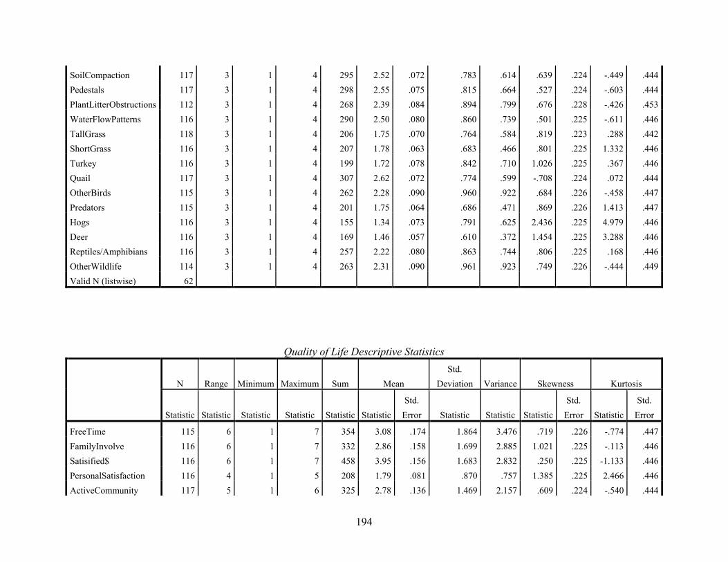
SoilCompaction 117 3 1 4 295 2.52 .072 .783 .614 .639 .224 -.449 .444 Pedestals 117 3 1 4 298 2.55 .075 .815 .664 .527 .224 -.603 .444 PlantLitterObstructions 112 3 1 4 268 2.39 .084 .894 .799 .676 .228 -.426 .453 WaterFlowPatterns 116 3 1 4 290 2.50 .080 .860 .739 .501 .225 -.611 .446 TallGrass 118 3 1 4 206 1.75 .070 .764 .584 .819 .223 .288 .442 ShortGrass 116 3 1 4 207 1.78 .063 .683 .466 .801 .225 1.332 .446 Turkey 116 3 1 4 199 1.72 .078 .842 .710 1.026 .225 .367 .446 Quail 117 3 1 4 307 2.62 .072 .774 .599 -.708 .224 .072 .444 OtherBirds 115 3 1 4 262 2.28 .090 .960 .922 .684 .226 -.458 .447 Predators 115 3 1 4 201 1.75 .064 .686 .471 .869 .226 1.413 .447 Hogs 116 3 1 4 155 1.34 .073 .791 .625 2.436 .225 4.979 .446 Deer 116 3 1 4 169 1.46 .057 .610 .372 1.454 .225 3.288 .446 Reptiles/Amphibians 116 3 1 4 257 2.22 .080 .863 .744 .806 .225 .168 .446 OtherWildlife 114 3 1 4 263 2.31 .090 .961 .923 .749 .226 -.444 .449 Valid N (listwise) 62
Quality of Life Descriptive Statistics
N Range Minimum Maximum Sum Mean
Std. Deviation Variance Skewness Kurtosis
Statistic Statistic Statistic Statistic Statistic Statistic Std.
Error Statistic Statistic Statistic Std.
Error Statistic Std.
Error
FreeTime 115 6 1 7 354 3.08 .174 1.864 3.476 .719 .226 -.774 .447 FamilyInvolve 116 6 1 7 332 2.86 .158 1.699 2.885 1.021 .225 -.113 .446 Satisified$ 116 6 1 7 458 3.95 .156 1.683 2.832 .250 .225 -1.133 .446 PersonalSatisfaction 116 4 1 5 208 1.79 .081 .870 .757 1.385 .225 2.466 .446 ActiveCommunity 117 5 1 6 325 2.78 .136 1.469 2.157 .609 .224 -.540 .444
194
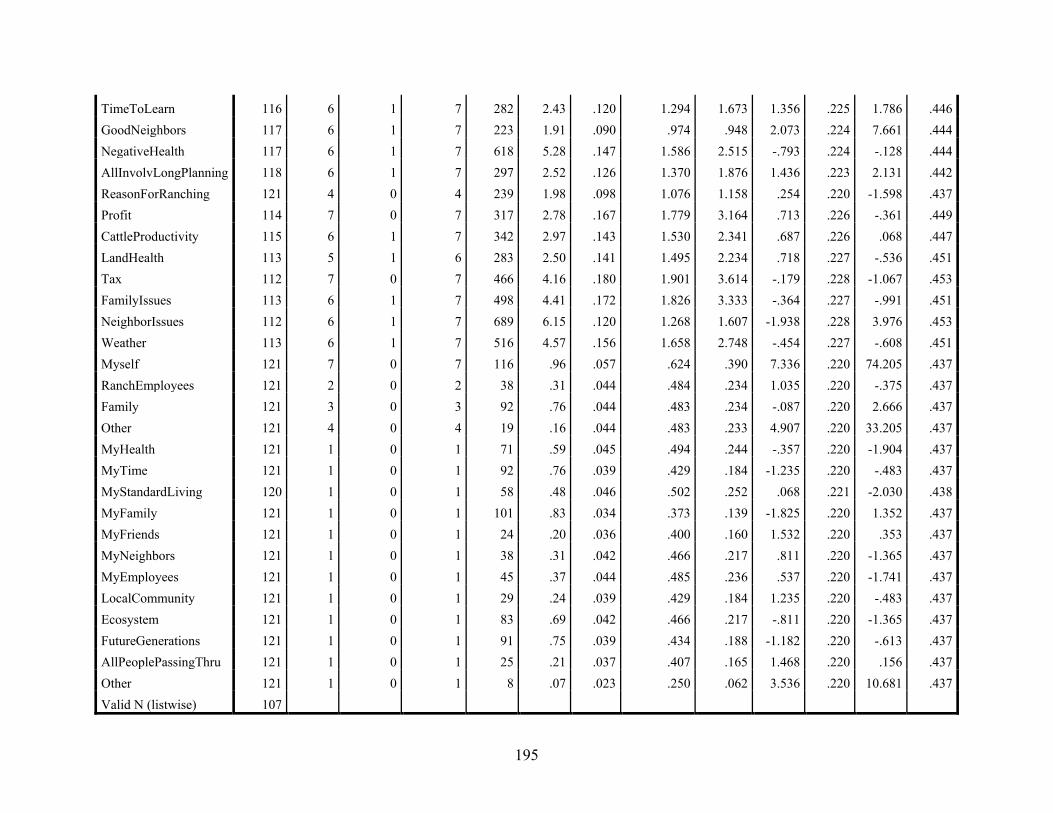
TimeToLearn 116 6 1 7 282 2.43 .120 1.294 1.673 1.356 .225 1.786 .446 GoodNeighbors 117 6 1 7 223 1.91 .090 .974 .948 2.073 .224 7.661 .444 NegativeHealth 117 6 1 7 618 5.28 .147 1.586 2.515 -.793 .224 -.128 .444 AllInvolvLongPlanning 118 6 1 7 297 2.52 .126 1.370 1.876 1.436 .223 2.131 .442 ReasonForRanching 121 4 0 4 239 1.98 .098 1.076 1.158 .254 .220 -1.598 .437 Profit 114 7 0 7 317 2.78 .167 1.779 3.164 .713 .226 -.361 .449 CattleProductivity 115 6 1 7 342 2.97 .143 1.530 2.341 .687 .226 .068 .447 LandHealth 113 5 1 6 283 2.50 .141 1.495 2.234 .718 .227 -.536 .451 Tax 112 7 0 7 466 4.16 .180 1.901 3.614 -.179 .228 -1.067 .453 FamilyIssues 113 6 1 7 498 4.41 .172 1.826 3.333 -.364 .227 -.991 .451 NeighborIssues 112 6 1 7 689 6.15 .120 1.268 1.607 -1.938 .228 3.976 .453 Weather 113 6 1 7 516 4.57 .156 1.658 2.748 -.454 .227 -.608 .451 Myself 121 7 0 7 116 .96 .057 .624 .390 7.336 .220 74.205 .437 RanchEmployees 121 2 0 2 38 .31 .044 .484 .234 1.035 .220 -.375 .437 Family 121 3 0 3 92 .76 .044 .483 .234 -.087 .220 2.666 .437 Other 121 4 0 4 19 .16 .044 .483 .233 4.907 .220 33.205 .437 MyHealth 121 1 0 1 71 .59 .045 .494 .244 -.357 .220 -1.904 .437 MyTime 121 1 0 1 92 .76 .039 .429 .184 -1.235 .220 -.483 .437 MyStandardLiving 120 1 0 1 58 .48 .046 .502 .252 .068 .221 -2.030 .438 MyFamily 121 1 0 1 101 .83 .034 .373 .139 -1.825 .220 1.352 .437 MyFriends 121 1 0 1 24 .20 .036 .400 .160 1.532 .220 .353 .437 MyNeighbors 121 1 0 1 38 .31 .042 .466 .217 .811 .220 -1.365 .437 MyEmployees 121 1 0 1 45 .37 .044 .485 .236 .537 .220 -1.741 .437 LocalCommunity 121 1 0 1 29 .24 .039 .429 .184 1.235 .220 -.483 .437 Ecosystem 121 1 0 1 83 .69 .042 .466 .217 -.811 .220 -1.365 .437 FutureGenerations 121 1 0 1 91 .75 .039 .434 .188 -1.182 .220 -.613 .437 AllPeoplePassingThru 121 1 0 1 25 .21 .037 .407 .165 1.468 .220 .156 .437 Other 121 1 0 1 8 .07 .023 .250 .062 3.536 .220 10.681 .437 Valid N (listwise) 107
195
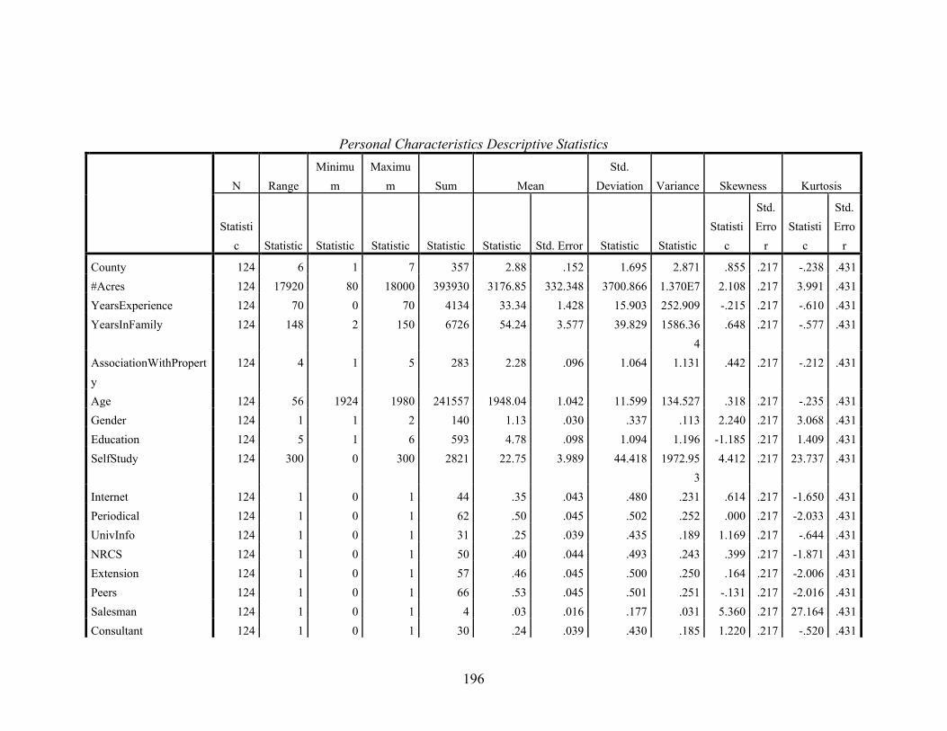
Personal Characteristics Descriptive Statistics
N Range
Minimum
Maximum Sum Mean
Std. Deviation Variance Skewness Kurtosis
Statistic Statistic Statistic Statistic Statistic Statistic Std. Error Statistic Statistic
Statistic
Std. Erro
r Statisti
c
Std. Erro
r
County 124 6 1 7 357 2.88 .152 1.695 2.871 .855 .217 -.238 .431 #Acres 124 17920 80 18000 393930 3176.85 332.348 3700.866 1.370E7 2.108 .217 3.991 .431 YearsExperience 124 70 0 70 4134 33.34 1.428 15.903 252.909 -.215 .217 -.610 .431 YearsInFamily 124 148 2 150 6726 54.24 3.577 39.829 1586.36
4 .648 .217 -.577 .431
AssociationWithProperty
124 4 1 5 283 2.28 .096 1.064 1.131 .442 .217 -.212 .431
Age 124 56 1924 1980 241557 1948.04 1.042 11.599 134.527 .318 .217 -.235 .431 Gender 124 1 1 2 140 1.13 .030 .337 .113 2.240 .217 3.068 .431 Education 124 5 1 6 593 4.78 .098 1.094 1.196 -1.185 .217 1.409 .431 SelfStudy 124 300 0 300 2821 22.75 3.989 44.418 1972.95
3 4.412 .217 23.737 .431
Internet 124 1 0 1 44 .35 .043 .480 .231 .614 .217 -1.650 .431 Periodical 124 1 0 1 62 .50 .045 .502 .252 .000 .217 -2.033 .431 UnivInfo 124 1 0 1 31 .25 .039 .435 .189 1.169 .217 -.644 .431 NRCS 124 1 0 1 50 .40 .044 .493 .243 .399 .217 -1.871 .431 Extension 124 1 0 1 57 .46 .045 .500 .250 .164 .217 -2.006 .431 Peers 124 1 0 1 66 .53 .045 .501 .251 -.131 .217 -2.016 .431 Salesman 124 1 0 1 4 .03 .016 .177 .031 5.360 .217 27.164 .431 Consultant 124 1 0 1 30 .24 .039 .430 .185 1.220 .217 -.520 .431
196
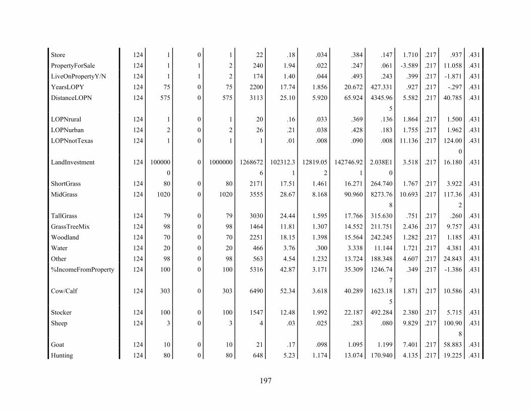
Store 124 1 0 1 22 .18 .034 .384 .147 1.710 .217 .937 .431 PropertyForSale 124 1 1 2 240 1.94 .022 .247 .061 -3.589 .217 11.058 .431 LiveOnPropertyY/N 124 1 1 2 174 1.40 .044 .493 .243 .399 .217 -1.871 .431 YearsLOPY 124 75 0 75 2200 17.74 1.856 20.672 427.331 .927 .217 -.297 .431 DistanceLOPN 124 575 0 575 3113 25.10 5.920 65.924 4345.96
5 5.582 .217 40.785 .431
LOPNrural 124 1 0 1 20 .16 .033 .369 .136 1.864 .217 1.500 .431 LOPNurban 124 2 0 2 26 .21 .038 .428 .183 1.755 .217 1.962 .431 LOPNnotTexas 124 1 0 1 1 .01 .008 .090 .008 11.136 .217 124.00
0 .431
LandInvestment 124 1000000
0 1000000 12686726
102312.31
12819.052
142746.921
2.038E10
3.518 .217 16.180 .431
ShortGrass 124 80 0 80 2171 17.51 1.461 16.271 264.740 1.767 .217 3.922 .431 MidGrass 124 1020 0 1020 3555 28.67 8.168 90.960 8273.76
8 10.693 .217 117.36
2 .431
TallGrass 124 79 0 79 3030 24.44 1.595 17.766 315.630 .751 .217 .260 .431 GrassTreeMix 124 98 0 98 1464 11.81 1.307 14.552 211.751 2.436 .217 9.757 .431 Woodland 124 70 0 70 2251 18.15 1.398 15.564 242.245 1.282 .217 1.185 .431 Water 124 20 0 20 466 3.76 .300 3.338 11.144 1.721 .217 4.381 .431 Other 124 98 0 98 563 4.54 1.232 13.724 188.348 4.607 .217 24.843 .431 %IncomeFromProperty 124 100 0 100 5316 42.87 3.171 35.309 1246.74
7 .349 .217 -1.386 .431
Cow/Calf 124 303 0 303 6490 52.34 3.618 40.289 1623.185
1.871 .217 10.586 .431
Stocker 124 100 0 100 1547 12.48 1.992 22.187 492.284 2.380 .217 5.715 .431 Sheep 124 3 0 3 4 .03 .025 .283 .080 9.829 .217 100.90
8 .431
Goat 124 10 0 10 21 .17 .098 1.095 1.199 7.401 .217 58.883 .431 Hunting 124 80 0 80 648 5.23 1.174 13.074 170.940 4.135 .217 19.225 .431
197
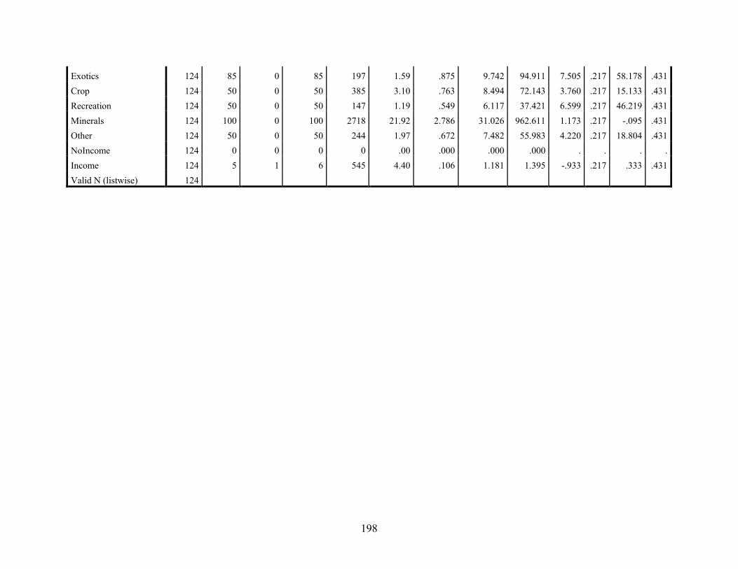
Exotics 124 85 0 85 197 1.59 .875 9.742 94.911 7.505 .217 58.178 .431 Crop 124 50 0 50 385 3.10 .763 8.494 72.143 3.760 .217 15.133 .431 Recreation 124 50 0 50 147 1.19 .549 6.117 37.421 6.599 .217 46.219 .431 Minerals 124 100 0 100 2718 21.92 2.786 31.026 962.611 1.173 .217 -.095 .431 Other 124 50 0 50 244 1.97 .672 7.482 55.983 4.220 .217 18.804 .431 NoIncome 124 0 0 0 0 .00 .000 .000 .000 . . . . Income 124 5 1 6 545 4.40 .106 1.181 1.395 -.933 .217 .333 .431 Valid N (listwise) 124
198
REFERENCE LIST
Abdel-Magid, A. H., Schuman, G. E., Hart, & R. H.Source. (1987). Soil bulk density and water infiltration as affected by grazing systems. Journal of Range Management, 40(4), 307-309.
Abrams, D. R. (2007). Introduction to regression. Retrieved [4/02/2011] http://dss.princeton.edu/online_help/analysis/regression_intro.htm#assum
Allen, R. & Harris, V. (2005). What we know about the demographics of U.S. farm operators.
Retrieved [1/30/2008] http://www.agcensus.usda.gov/Publications/2002/Other_Analysis/index.asp
Allred, K.W. (1996). Vegetative changes in New Mexico rangelands. New Mexico Journal of Science, 36, 168–231.
Ash, A.J. & Stafford-Smith, D.M. (1996). Evaluating stocking rate impacts in rangelands: animals don‘t practice what we preach. Rangeland Journal, 18(2), 216-243.
Atkinson, P.W., Fuller, R.J. Vickery, J.A. Conway, G.J. Tallowin, J.R.B. Smith, R.E.N. Haysom, K.A. Ings, T.C. Asteraki, E.J. & Brown, V.K. (2005). Influence of agricultural management, sward structure and food resources on grassland field use by birds in lowland England. Journal of Applied Ecology, 42, 932–942.
Bailey, D.W., Provenza, F.D. (2008). Mechanisms determining large-herbivore distribution. In: Prins, H.T.T. & van Langevelde, F. (Eds.), Resource Ecology: Spatial and Temporal Dynamics of Foraging (pp. 7–28). Dordrecht, Netherlands: Springer.
Bailey D.W., Gross, J.E., Laca, E.A., Rittenhouse, L.R., Coughenour, M.B., Swift, D.M., & Sims, P.L. (1996). Mechanisms that result in large herbivore grazing patterns. Journal of Range Management, 49, 386-400.
Bakker, J.P. & Berendse, F. (1999). Constraints in the restoration of ecological diversity in grassland and heathland communities. Trends in Ecology &. Evolution, 14, 63–68.
Bartlett, E.T., Maczko, K.A., & Mitchell. J.E. (2003). Ecological, economic, and social indicators: assessing rangeland sustainability. (pp. 1897-1908). In: Allsopp, N., Palmer, A.R., Milton, S.J., Kirkman, K.P., Kerley, G.I.H., & Hurt, C.R. (eds.) Proc. VIIth Int. Rangeland Congress, (26th July-Ist August 2003), Durban, South Africa: Document Transformation Technologies, Irene, South Africa.
Becker, G. S. (1974). A theory of social interactions. Journal of Political Economy, 82(6),1063–1093.
Beem, M. (2010). Absentee rural land ownership [Oklahoma Cooperative Extension publication AGEC-966]. Retrieved [7/12/2011] http://www.absenteelandowners.org/info-for-landowners
199
Beeskow, A.M., Elissalde, N. O., & Rostagno, C. M. (1995). Ecosystem changes associated with grazing intensity on the Punta Ninfas rangelands of Patagonia, Argintina. Journal of Range Management, 48(6), 517-522.
Belsky, A.J. (1986). Does herbivory benefit plants? A review of the evidence. American Naturalist, 127, 870-892.
Belsky, A.J., Matzke, A., & Uselman, S. (1999). Survey of livestock influences on stream and riparian ecosystems in the western United States. Journal of Soil and Water Conservation, 54, 419-432.
Bland J.M., Altman, D.G. (1997). Statistics notes: Cronbach's alpha. BMJ, 1997, 314 - 572 Bollig, M., & Schulte, A. (1999). Environmental change and pastoral perceptions: indigenous
knowledge in two degradation and African pastoral communities. Human Ecology, 27, 493–514.
Booth, M.S., Stark, J.M., & Caldwell, M.M. (2003). Inorganic N turnover and availability in annual and perennial dominated soils in a northern Utah shrub-steppe ecosystem . Biogeochemistry, 66, 311-330.
Booysen, P. deV. & Tainton, N.M. (1978). Grassland management: principles and practice in South Africa. (pp. 551-554). Proceedings 1st International Rangeland Congress. Denver, Colorado.
Bradford, D. (1998). Holistic resource management in the West Elks: why it works. Rangelands. 20, 6-9.
Briske, D. D. & Anderson, V. J. (1990). Tiller dispersion in populations of the bunchgrass Schizachyrium Scoparium: Implications for herbivory tolerance. Oikos, 59, 50-56.
Briske, D. D., Derner, J. D. Brown, J. R., Fuhlendorf, S. D., Teague, W. R., Havstad, K. M.,
Gillen, R. L., Ash, A. J. & Willms, W. D. (2008). Rotational grazing on rangelands: reconciliation of perception and experimental evidence. Rangeland Ecology & Management, 61, 3–17.
Brunson, M.W. (2003). Rangelands and society. Rangelands, 25(6), 16-21.
Buckhouse, J.C., Busby, F.E., Clanton, D.C., Coggins, G.C., & Evans, G.R. (1994). New methods to classify, inventory, and monitor rangelands. Available from http://www.nap.edu/openbook.php?isbn=0309048796
Buckingham, D.L., Peach, W.J. & Fox, D.S. (2006). Effects of lowland agricultural management on the use of lowland grassland by foraging birds. Agriculture Ecosystem & Environment, 112, 21–40.
Buffington LC, Herbel, C.H. (1965) Vegetation changes on a semi-desert grassland range from 1858–1964. Ecological Monographs, 35, 139–164.
200
Butler, L. (2002). Economic survival of western ranching: searching for an answer. In: Knight, R. L., Gigert, W.C., Marston, E. (ed), Ranching West of the 100th Meridian: Culture, Ecology and Economics (pp. 195-202). Washington DC: Island Press.
Butterfield, J., Bingham, S., Savory, A. (2006). Holistic Management Handbook: Healthy Land, Healthy Profits. Washington DC: Island Press.
Calker, K.J. (2005). Sustainability of Dutch dairy farming systems: a modeling approach. (Doctoral dissertation). Retrieved from Wageningen Universiteit. http://edepot.wur.nl/36804
Callicott, J.B. (1991). The wilderness idea revisited: the sustainable development alternative. In: Callicott, J.B. and Nelson, M.P. (Ed.). The Great New Wilderness Debate (p. 345). Athens Georgia: The University of Georgia Press.
Cattell, R. B. (1966). The scree test for thenumber of factors. Multivariate Behavioral Research, 1, 245-276.
Centeri, C., E. Herczeg, M., Vona, K. Balazs, and K. Penksza. (2009). The effects of land-use change on plant–soil–erosion relations, Nyereg Hill, Hungary Journal of Plant Nutrition and Soil Science, 172, 586-592.
Chouinard, H.H., Paterson, T., Wandschneider, P.R., Ohler, A.M. (2008). Will farmers trade profits for stewardship? Heterogeneous motivations for farm practice selection. Land Economics, 84(1), 66-82.
Christensen, L.M. Coughernour, B. Ellis, J.E. & Chen, Z. (2003). Sustainability of inner Mongolian grasslands: application of the savanna model. Journal of Range Management. 56(4), 319-327.
Clark, E.A., & Weise, S.F. (1993). A forage-based vision of sustainable agriculture. Proc. 92nd Symp. NE Branch, American Society of Agronomy: Madison, WI.
Committee on Rangeland Classification. (1994). Rangeland Health: New Methods To Classify, Inventory And Monitor Range-Lands. Washington, DC: Nat. Acad. Press.
Conner, J.R. (1991). Social and economic influences on grazing management. Heitschmidt, R.K. & Stuth, J.W. (ed). In: Grazing Management: An Ecological Perspective (pp. 191–200). Portland, O: Timber Press, Inc.
Cordell, H.K. & Overdevest, C. (2001). Footprints on the land: an assessment of demographic trends and the future of natural lands in the United States. Champaign, Ill: Sagamore Publ.
Costa, F.P. & Reham, T. (2005). Unraveling the rationale of ‗overgrazing' and stocking rates in the beef production systems of Central Brazil using a bi-criteria compromise programming model. Agricultural Systems, 83(3), 277-295.
201
Coughenour, M.B., McNaughton S.J. & Wallace, L.L. (1985). Responses of an African graminoid (Themeda triandra Forsk.) to frequent defoliation, nitrogen and water: A limit of the adaptation to herbivory. Oecologia, 68, 105-111.
Coughenour, M.B. (1991). Spatial components of plant-herbivor interactions in pastoral, ranching, and native ungulate ecosystems. Journal of Range Management, 44, 530-542.
Crawley, M.J. ( 1987). Benevolent herbivores? Trends in Ecology and Evolution, 2, 167-168.
Crider, F.J. (1955). Root-growth stoppage resulting from defoliation of grass. (USDA Tech. Bull. 1102). Washington DC: United States Department of Agriculture.
Cronbach, L. J. (1951). Coefficient alpha and the internal structure of tests. Psychometrika,
16(3), 297-334.
Dagget, D., & Dusard, J. (1995). Beyond the Rangeland Conflict: Toward a West that Works. Flagstaff AZ: The Grand Canyon Trust.
Danckwerts, J.E., O‘Reagain, P.J. & O‘Connor, T.G. (1993). Range management in a changing environment: a southern African perspective. Rangeland Journal, 15, 133-144.
Daugherty, D.A., Britton, C.M. & Turner, H.A. (1982). Grazing management of crested wheatgrass range for yearling steers. Journal of Range Management, 35, 347-351.
Davis, Walt. (1996). When values run your ranch. (Spring. p. 3-4.) In: The Holistic Resource Management Quarterly. Albuquerque, NM: Holistic Management International.
de Leeuw, J. (1988). Multivariate analysis with linearizable regressions. Psychometrika, 53, 437- 454.
de Leeuw J, Michailidis G, Wang, D.Y. (1999). Correspondence analysis techniques. S Ghosh (ed.), Multivariate Analysis, Design of Experiments, and Survey Sampling (pp. 523-546). New York, NY: Dekker.
de Leeuw , J., & Mair, P. (2010). A General Framework for Multivariate Analysis with Optimal Scaling: The R Package aspect. Journal of Statistical Software, 32(9), 1-23. URL http://www.jstatsoft.org/v32/i09/.
Dennis, P, Young, M.R., & Gordon, I.J. (1998). Distribution and abundance of small insects and arachnids in relation to structural heterogeneity of grazed indigenous grasslands. Ecological Entomology, 23, 253–264.
Deregibus, V.A., Jacobo1, E., & Ansin, O.E. (2001). Grassland use and plant diversity in grazed ecosystems. Proceeding of the XIX International Grassland Conf. Sao Paulo, Brazil.
Derner, J.D., Gillen, R.L., McCollum, F.T., & Tate. K.W. (1994). Little bluestem tiller defoliation patterns under continuous and rotational grazing. Journal of Range Management, 47, 220-225.
202
Diaz-Solis, H., Kothmann, M.M., Grant, W.E., De Luna-Vilarreal, R. (2006). Application of a simple ecological sustainability simulator (SESS) as a management tool in the semi-arid rangelands of northeastern Mexico. Agricultural Systems, 88(2-3), 514-527.
Dillman, C.A. (2000). Mail and Internet surveys: The tailored design method. 2nd ed. New York, NY: John Wiley and Sons.
Doll, J.E. & Jackson, R.D. (2009). Wisconsin farmer attitudes regarding native grass us in grazing systems. Journal of Soil and Water Conservation. 64(4), 276-285.
Dudley, J.P. (1997). Paleontological and cultural perspectives on livestock grazing in southwestern rangelands: response to Brown and McDonald‖. Conservation Biology, 11 (1), 267-269.
Earl, J.M. & Jones, C.E. (1996). The need for a new approach to grazing management - is cell grazing the answer? The Rangeland Journal, 18, 327-350.
FAO. (1991). Sustainable agriculture and rural development, in Asia and the Pacific (p. 24). Regional Document No. 2. FAO/Netherlands Conference on Agriculture and the Environment: Hertogenbosch, the Netherlands.
Field, A. (2005). Discovering Statistics Using SPSS (and sex, drugs, and rock’n roll). Ltd; 2nd edition UK: Sage Publications.
Fleischner, T.L. (1994). Ecological Costs of Livestock Grazing in Western North America. Conservation Biology, 8, 629-644.
Foreman, D. (1991). Confessions of an Eco-Warrior. New York, NY: Harmony Books.
Fowler, J.M., & Gray, J.R. (1986). Economic impacts of grazing systems during drought and nondrought years on cattle and sheep ranches in New Mexico. (N. Mex. Agric. Exp. Stn. Bull. 725). Las Cruces, NM: New Mexico State University.
Frank, D.A. & Groffman, P.A. (1998). Ungulate vs. landscape control of soil C and N processes in grasslands of Yellowstone National Park. Ecology, 79, 2229-2241.
Frank, D.A., & McNaughton, S.J. (1993). Evidence for the promotion of aboveground grassland production by native large herbivores in Yellowstone National Park. Oecologia, 96, 157-161.
Frank, D.A., Kuns, M.M., & Guido, D.R. (2002). Consumer Control of Grassland Plant Production. Ecology, 83, 602-606.
Frank,D.A. & McNaughton, S.J. (2002). The ecology of the earth‘s grazing ecosystems. BioScience, 48, 513-521.
Fuhlendorf, S.D & Smins, F.E. (1998). The influence of soil depth on plant species response to grazing within a semi-arid savanna. Plant Ecology, 138(1), 89-96.
203
Fuhlendorf, S.D. & Engle, D.M. (2001). Restoring heterogeneity on rangelands: ecosystem management based on evolutionary grazing patterns. Bioscience, 51, 625-632
Fuhlendorf, S.D., Harrell, W.C., Engle, D.M. Hamilton, R.G., Davis, C.A., & Leslie Jr., D.M. (2006). Should heterogeneity be the basis for conservation? Grassland bird response to fire and grazing. Ecological Applications, 16 (5), 1706-1716.
Garson, G.D. (2011a). "Scales and Standard Measures", from Statnotes: Topics in Multivariate Analysis. Retrieved (5/12/2011) from http://faculty.chass.ncsu.edu/garson/pa765/statnote.htm.
Garson, G.D. (2011b). Factor analysis. from Statnotes: Topics in Multivariate Analysis. Retrieved [5/19/2011] from http://faculty.chass.ncsu.edu/garson/pa765/statnote.htm.
Garson, G.D. (2011c). Testing of assumptions, from Statnotes: Topics in Multivariate Analysis. Retrieved [5/19/2011] from http://faculty.chass.ncsu.edu/garson/pa765/statnote.htm.
Garson, G.D. (2011d). Multiple regression, from Statnotes: Topics in Multivariate Analysis. Retrieved [5/19/2011] from http://faculty.chass.ncsu.edu/garson/PA765/regress.htm.
Garson, G.D. (2011e). Testing of assumptions, from Statnotes: Topics in Multivariate Analysis. Retrieved [6/01/2011] from http://faculty.chass.ncsu.edu/garson/PA765/regress.htm.
Gelman, A., & Hill, J. (2006). Data analysis using regression and multilevel/hierarchical models (Chapter 25). Retrieved [3/2/2011] http://www.stat.columbia.edu/~gelman/arm/missing.pdf : Cambridge University Press
Gibbens, R.P, McNeely, R.P, Havstad, K.M, Beck, R.F, & Nolen, B. (2005) Vegetation changes in the Jornada Basin from 1858–1998. Journal of Arid Environments, 61, 651–668.
Gray, J.R., and J.M. Fowler. (1980). Requirements for economic analysis of grazing systems. In: Proc. Grazing Management Systems for Southwest Rangelands Symposium. The Range Improvement Task Force, New Mexico Sate University, Las Cruces, N. Mex.
Greiner, R., Patterson, L., & Miller, O. (2008). The role of grazier motivations and risk attitudes in the adoption of grazing best management practices. Proceedings from 52nd Annual Conference of the Australian Agricultural and Resource Economics Society. Canberra. Australia.
Greiner, R., Patterson, L., & Miller, O. (2009). Motivations, risk perceptions and adoption of conservation practices by farmers. Agricultural Systems, 99, 86-104.
Hair, J.F., I Anderson, R. Jr., Tatham, R.L. & Black, W.C. (1998). Multivariate data analysis with readings, 5th ed. Englewood Cliffs, NJ: Prentice-Hall.
Hamilton, E.W. & Frank., D.A. (2001). Can plants stimulate soil microbes and their own nutrient supply? Evidence from a grazing tolerant grass. Ecology, 82, 2397-2402.
Hanselka, C.W. (2007). What is holistic resource management? Retrieved [3/16/07] http://hrm-texas.org/what_is_HRM.htm.
204
Hanselka, W., Lyons, R., & Mosley, M. (2009). Grazing Land Stewardship. Winn, J (Ed.). (Publication B-6221). College Station, TX: Texas AgriLife Extension Service.
Hart, R.H., Samuel, M.J. Test, P. S. & Smith, M.A. (1988). Cattle, vegetation, and economic responses to grazing systems and grazing pressure. Journal of Range Management, 41, 282–288.
Hastie, T., Tibshirani, R., Sherlock, G., Eisen, M., Brown, P., & Botstein, D. (1999). Imputing missing data for gene expression arrays. Stanford University Statistics Department Technical report. Retrieved [4/5/2011] http://www-stat.stanford.edu/~hastie/Papers/missing.pdf.
Heitschmidt, R.K., & Taylor, C.A. Jr. (1991). Livestock production (p. 161-177). In: Heitschmidt, R.K. & Stuth, J.W. (Editors). Grazing Management: An Ecological Perspective. Portland OR: Timber Press.
Heitschmidt, R.K., Conner, J.R., Canon, S.K., Pinchak, W.E., Walker, J.W. & Dowhower, S.L. (1990). Cow/calf production and economic returns from yearlong continuous, deferred rotation and rotational grazing treatments. Journal of Production Agriculture, 3, 92-99.
Heitschmidt, R.K., Vermeire, L.T. & Grings, E.E. (2004). Is rangeland agriculture sustainable? Journal of Animal Science, 82, 138-146.
Hobbs, N.T. & Swift, D.M. (1988). Grazing in herds: when are nutritional benefits realized? American Naturalist, 131, 760-764.
Holechek, J.L. (1984). Comparative contribution of grasses, forbs and shrubs t the nutrition of range ungulates. Rangelands, 6(6), 261-263.
Holechek, J.L., Pieper, R.D., & Herbel, C.H. (1989). Range Management Principles and Practices. Upper Saddle River, NJ: Prentice Hall.
Holechek, J.L. (1992). Financial benefits of range management practices in the Chihuahuan desert. Rangelands, 14(5):279–284.
Holechek, J.L., Tembo, A. Daniel, A., Fusco, M., & Cardenas, M. (1994). Long term grazing influences on chihuahuan desert rangeland. Southwestern Naturalist, 39, 342-349.
Holland, E.A., Paron, W.J., Detling, J.K., & Coppock, D.L. (1992). Physiological responses of plant populations to herbivory and their consequences for ecosystem nutrient flow. American Naturalist, 140(4), 685-706.
Hormay, A.L. (1956). How livestock grazing habits and growth requirements of range plants determine sound grazing management. Journal of Range Management, 9, 161-164.
Hormay, A.L. (1970). Principles of rest-rotation grazing and multiple-use management (USDA For. Serv. Training Text 4). Washington, DC: United States Department of Agriculture.
205
Hormay, A.L. & Evanko, A.B. (1958). Rest-rotation grazing …a management system for bunchgrass ranges (California Forest and Range Experiment Station. Misc. Paper 27). Washington, DC: USDA Forest Service.
Hormay, A.L. & Talbot. M.W. (1961). Rest-rotation grazing …a new management system for perennial bunchgrass ranges (USDA Forest Service, Research Report 51). Washington, DC: USDA Forest Service.
Horn, J.L. (1965). A rationale and test for the number of factors in factor analysis, Psychometrika, 30, 179-85.
Howell, J., Miller, P., Park, H.H., Sattler, D., Schack, T., Spery, E., Widhalm, S., & Palmquist, M. (2005). Reliability and Validity. Colorado State University Department of English. Retrieved [1/12/2011] from http://writing.colostate.edu/guides/research/relval/.
Hughes, L.E. (1983). Is no grazing really better than grazing? Rangelands, 5, 159-161.
Hunt, L.P., Petty, S., Crowley, R., Fisher, A., Ash, A.J. & MacDonald, N. (2007). Factors affecting management of cattle grazing distribution in northern Australia: preliminary observations on the effect of paddock size and water points. Rangeland Journal, 29, 169-179.
Johnson, B.H., (Ed.). (2003). Forging a West that Works: An Invitation to the Radical Center. Santa Fe NM: Quivira Coalition.
Jung, H.G., R.W. Rice, and L.J. Koong. (1985). Comparison of heifer weight gains and forage quality for continuous and short-duration grazing systems. Journal of Range Management, 38, 144-149.
Kaiser, H.F. (1974) An index of factorial simplicity. Psychometrika, 39, 31-36.
Karahoca, D., Karahoca, A., Karaoglu, A., Gulluoglu, B., & Arifoglu, E. (2010). Evaluation of web based learning on student achievement in primary school computer courses. Procedia - Social and Behavioral Science, 2(2), 5813-5819.
Kim, K.Y., Kim, B., & Yi, G.S. (2004). Reuse of imputed data in microarray analysis increases imputation efficiency, BMC Bioinformatics, 5, 160.
Kim, K.Y. & Yi, G.S. (2008). Sequential KNN imputation method. Retrieved [2/12/2011] http://cran.r-project.org/SeqKNN/index.html.
Kim, K., & Yi, G. (2009). Package ‘SeqKnn’. Available at:http://cran.r-project.org/web/packages/SeqKnn/SeqKnn.pdf.
Klipple, G.E. & Costello, D.F. (1960). Vegetation and cattle responses to different intensities of grazing on shortgrass ranges of the central great plains (USDA Tech. Bull. 1216). Washington, DC: United States Department of Agriculture.
206
Knapp, A.K., Blair, J.M., Briggs, J.M., Collins, S.L., Hartnett, D.C., Johnson, L.C., & Towne, E.G. (1999). The keystone role of bison in North American tallgrass prairie. BioScience, 49, 39–50.
Knapp, N.C. & Fernandez-Gimenez, M.E. (2009). Knowledge in practice: documenting rancher local knowledge in northwest colorado. Rangeland Ecology & Management, 62, 500-509.
Knight, R. L., Gigert, W.C., Marston, E. (Ed.). (2002). Ranching West of the 100th Meridian: Culture, Ecology and Economics. Washington DC: Island Press.
Knight, R. W., & Heightschmidt., R. K. (1987). Infiltration rates and sediment production as influenced by grazing systems in the Texas Rolling Plains‖ Journal of Range Management, 40(3), 240-243.
Kothmann, M.M., Mathis, G.W., & Waldrip, W.J. (1971). Cow-calf response to stocking rates and grazing systems on native range. Journal of Range Management, 14, 57-62.
Kreuter, U., Nair, M., & Jackson-Smith, D. (2006). Property rights orientations and rangeland management practices: Texas, Utah and Colorado. Rangeland Ecology & Management, 59, 632-639.
Laca, E.A. (2009). New approaches and tools for grazing management. Rangeland Ecology & Management, 62, 407-417.
Lal, R. (2003). Soil erosion and the global carbon budget, Environment International, 29, 437–450.
Lancaster, K.J. (1966). A new approach to consumer theory. Journal of Political Economy, 74, 132–157.
Launchbaugh, J.L. (1986). Intensive-early season stocking. Proceedings of the Ranch Management Symposium (November 5-7), North Platte, Nebraska.
Law, F. (2009). Global Harvest urges food production increases. Southwest Farm Press. Retrieved from [10/21/2009] http://southwestfarmpress.com/news/global-harvest-1021/.
Leontitsis, A., & Pagge, J. (2007). A simulation approach on Cronbach's alpha statistical significance. Mathematics and Computers in Simulation, 73(5), 336-340.
Leopold, A. (1938). The River of the Mother of God and Other Essays by Aldo Leopold. Madison, WI: Univ. Wisconsin Press,
Leopold, A. (1949). A Sand County Almanac. Oxford England: Oxford University Press.
Li, J., Okin, G.S., Alvarez, & L. Epstein, H. (2007). Quantitative effects of vegetation cover on wind erosion and soil nutrient loss in a desert grassland of southern New Mexico, USA. Biogeochemistry, 85, 317–332.
Louda, S.M. (1990). Review: plant morphology and herbivory. Ecology, 71, 829-830.
207
Lowdermilk, W.C. (1953). Conquest of the Land through 7, 000 years. (USDA NRCS Agr. Info. Bull. No. 99). Washington, DC: United States Department of Agriculture.
Lubowiski , R.N., Vesterby, M., Bucholtz, S., Baez, A., & Roberts, M. J. (2006). (Economic Information Bulletin No. EIB-14). USDA Economic Research Service. Retrieved [7/17/2009] from http://www.ers.usda.gov/Publications/EIB14/.
Ludwig, J.A. & Tongway. (1995). Spatial organization of landscapes and its function in semi-arid woodlands in Australia. Landscape Ecology, 10(1) 51-63.
Mac Arthur, R.H., Diamond, J.M., & Karr, J.R. (1972). Density Compensation in island faunas. Ecology, 53, 2.
MacRae, R.J., Henning, J. & Hill, S.B. (1993). Strategies to overcome barriers to the development of sustainable agriculture in Canada: The role of agribusiness. Journal of Agriculture & Environmental Ethics, 6, 21–51.
Maczko, K. A., Bryant, L.D., Thompson, D.W., Borchard, S.J. (2004). Putting the pieces together: Assessing social, ecological, and economic rangeland sustainability. Rangelands, 26(3), 3-14.
Maczko. K., & Hidinger, L. (ed.). (2008). Sustainable Rangeland Ecosystem Goods and Services. Sustainable Rangeland Roundtable. Available at: http://sustainablerangelands.warnercnr.colostate.edu/.
Maindonald, J. (2011). Package ‘DAAG’. Available at CRAN: http://cran.r-project.org/web/packages/DAAG/index.html
Mair P, De Leeuw J. (2010). A General Framework for Multivariate Analysis with Optimal Scaling: The R Package aspect." Journal of Statistical Software, 32(9), Retrieved [5/14/2011]. http://www.jstatsoft.org/v32/i09/.
Marriott, C.A., Hood, K., Fisher, J.M., Pakeman, R.J. (2009). Long-term impacts of extensive grazing and abandonment on the species composition, richness, diversity and productivity of agricultural grassland. Agriculture, Ecosystems & Environment, 134(3-4) 190-200.
Maslow, A.H. (1954). Motivation and Personality. New York, NY: Harper and Row.
Matthews, E.D. (1954). Tukulu – a pioneer’s story. 2nd Edition, Grassland Society of Southern Africa, Pietermaritzburg, South Africa.
McCann, K.S. (2000). The diversity-stability debate. Nature, 405(6783), 228-33.
McIlvain, E.H., & Savage, D.A. (1951). Eight-year comparisons of continuous and rotational grzing on the southern plains range. Journal of Range Management, 4, 42-47.
McNaughton S.J., Oesterheld, M., Frank, D.A., & Williams, K.J. (1989). Ecosystem-level patterns of primary productivity and herbivory in terrestrial habitats. Nature , 341, 142-144.
208
McNaughton, S.J. (1979). Grazing as an optimization process: grass-ungulate relationships in the serengeti. The American Naturalist, 113, 691-703.
McQuarrie, A.D.R., & Tsai, C.L., (1998). Regression and Time Series Model Selection. River Edge, NJ: World Scientific Publishing Co. Pte. Ltd.
Merrill, L.B. (1954). A variation of deferred rotation grazing for use under southwest range conditions. Journal of Range Management, 7, 152-154.
Meulman, J.J. (1988). Optimal scaling methods for multivariate categorical data analysis. Data Theory Group Faculty of Social and Behavioral Sciences: Leiden University. Retrieved [5/2/2011] http://www.unt.edu/rss/class/Jon/SPSS_SC/Module9/M9_CatReg/SWPOPT.pdf
Michunas, D.G., Sala, O.E., & Lauenroth, W.K. (1988). A generalized model of the effects of grazing by large herbivores on grassland community structure. American Naturalist, 132, 87–106.
Moore, A. (2008). Cross-Validation [tutorial slides]. Available at: http://www.autonlab.org/tutorials/overfit.html
Moss, S. (2008). An overview of optimal scaling. Retrieved [5/10/2011] http://www.psych-it.com.au/Psychlopedia/article.asp?id=159.
Mowry, R. (2007). Overgrazing: bad for business, bad for biodiversity. Univ of Idaho. Retrieved [11/28/07] http://www.cnr.uidaho.edu/range456/hot-topics/Overgrazing.htm.
Müller, B., Frank, K. and Wissel, C. (2007). Relevance of rest periods in non-equilibrium rangeland systems - A modeling analysis. Agricultural systems, 92, 295-317.
Nabhan, G.P. (1995). Cultural Parallax in Viewing North American Habitats (p. 630). In: The Great New Wilderness Debate, Callicott, J.B. and Nelson, M.P. (ed). Athens, GA: The University of Georgia Press.
Naeem, S. (2002). Ecosystem consequences of biodiversity loss: the evolution of a paradigm. Ecology, 83, 1537–1552.
Naeth, M.A. and D.S. Chanasyk. (1995). Grazing effects on soil water in Alberta foothills fescue grasslands. Journal of Range Management, 48(6), 528-534.
Nash, R.F. (2001). Wilderness and the American Mind (p. 384). 4th edition. New Haven, CT: Yale University Press.
Norton, B.E. (1998). The application of grazing management to increase sustainable livestock production. Animal Production in Australia, 22, 15-26.
NRCS. (2000). Interpreting Indicators of Rangeland Health. (Technical Reference 1734-6. Version 3. pp. 3-9). Washington, DC: United States Department of Agriculture.
209
NRCS. (2003). National Range and Pasture Handbook. Retrieved [6/10/2011] http://www.glti.nrcs.usda.gov/technical/publications/nrph.html
Nunnaly, J.C. & Bernstein, I.H. (1994). Psychometric Theory (3rd ed.). New York, NY: McGraw-Hill.
O‘Connor, T.G. 1992. Patterns of plant selection by grazing cattle in two savanna grasslands: A plant‘s eye view. Journal of the Grassland Society of Southern Africa, 9, 97-104.
O‘Reagain, P., McKeon, G., Day, K., & Ash, A. (2003). Managing for temporal variability in extensive rangelands – a perspective from Northern Australia (pp 799-809). (July 26-August 1). Proceedings of the VIIth International Rangeland Congress. Durban, South Africa.
O'Connor, B. P. (2000). SPSS and SAS programs for determining the number of components using parallel analysis and Velicer's MAP test. Behavior Research Methods, Instruments and Computers, 32(3), 396-402.
Oesterheld, M., Sala, O.E., & McNaughton, S.J. (1992). Effect of animal husbandry on herbivore-carrying capacity at a regional scale. Nature, 1992, 234-236.
Ormerod, S. J, Marshall, E. J. P., Gillian Kerby & Rushton, S. P. (2003). Meeting the ecological challenges of agricultural change. Journal of Applied Ecology, 40(6), 939-946.
Patil, V.H., S.N. Singh, S. Mishra, and T. Donovan (2007), Parallel Analysis Engine to Aid Determining Number of Factors to Retain [Computer software]. Retrieved [5/3/20100] http://ires.ku.edu/~smishra/parallelengine.htm; Utility developed as part of Patil, V.H., S.N. Singh, S. Mishra, and T. Donovan (2008), Efficient theory development and factor retention criteria: A case for abandoning the ―eigenvalue greater than one‖ criterion, Journal of Business Research, 6 (2), 162-170.
Patil, V.H., Singh, S.N., Mishra, S. & Donovan, T. (2008). Efficient theory development and factor retention criteria: a case for abandoning the eigenvalue greater than one criterion. Journal of Business Research, 6 (2), 162-170.
Pickett, S.T.A. & White, P.S. (1985). Patch dynamics: a synthesis (pp. 371-384). In: Pickett, S.T.A., & White, P.S. The Ecology of Natural Disturbance and Patch Dynamics, New York, NY: Academic Press.
Pickup, G. & Stafford-Smith, D.M. (1993). Problems, prospects and procedures for assessing the sustainability of pastoral land management in Australia. Journal of Biogeography, 20, 471-487.
Pieper, R.D., Donart, G.B., Parker, E.E, & Wallace, J. D. (1978). Livesock and vegetational response to continuous and four-pasture one-herd grazing systems in New Mexico. Proc. Int. Rangel. Congr. 1, 560-562.
210
Pluhar, J.J., Knight, R.W., & Heitschmidt, R.K. (1987). Infiltration rates and sediment production as influenced by grazing systems in the Texas rolling plains. Journal of Range Management, 40(3), 240-243.
Polley, H.W. & Detling J.K. (1989). Defoliation, nitrogen and competition: Effects on plant growth and nitrogen nutrition. Ecology, 70, 721-727.
Pomerantz, J.R. (2003): Perception: Overview (pp. 527–537). In: Lynn Nadel (Ed.), Encyclopedia of Cognitive Science, London, GB: Nature Publishing Group.
Provenza, F.D. (2003a). Foraging behavior: Managing to survive in a world of change. Utah Agricultural Experiment Station, Retrieved [7/18/2010] http://behave.net/products/booklet.html.
Provenza, F.D. (2003b). Twenty-five years of paradox in plant-herbivore interactions and ―sustainable‖ grazing management. Rangelands, 25, 4-15.
R-2.13.0. (2011). The Comprehensive R Archive Network. Available at: http://cran.r-project.org/
Raether, K. (2002). Home on the holistic range. In: Watershed Messenger (Vol. 9). Hailey, ID: Western Watersheds Project.
Raftery A., Hoeting, J., Volinsky, C., Painter, I. Yeung, K.Y. (2011). Package ‘BMA’. Available at CRAN: http://cran.r-project.org/web/packages/BMA/index.html
Raftery, A.E. (1995). Bayesian model selection in social research (with Discussion) (pp. 111-196). In: Marsden, P.V. (Ed.). Sociological Methodology, Cambridge, Mass: Blackwells.
Raubenheimer, J.E. (2004). An item selection procedure to maximize scale reliability and validity. South African Journal of Industrial Psychology, 30 (4), 59-64.
Reardon, P.O. and L.B. Merrill. (1976). Vegetative response under various grazing management systems in the Edwards Plateau of Texas. Journal of Range Management, 29, 195-198.
Reece, P.A. (1986). Short-duration grazing research and case studies in Nebraska. In: Proc. Short-Duration Grazing and Current Issues in Grazing Management Shortcourse. Washinton State University Cooperative Extension Service, Pullman Wash.
Rogler, G.A. (1951). A twenty-five year comparison of continuous and rotation grazing in the northern plains. Journal of Range Management, 4, 35-41.
Rowan, R.C., White, L.D. & Conner, J.R. (1994). Understanding cause/effect relationships in stocking rate change over time. Journal of Range Management, 47, 349-354.
Sampson, A.W. (1913). Range improvement by deferred and rotation grazing (USDA Bull. 34). Washington, DC: U.S. Dept. of Agriculture.
211
Samson, F., Knopf, F.L., & Ostlie, W.R. (2004). Great Plains Ecosystems: Past, Present, and Future. BioScience, 51, 869-873.
Samuelson, P.A. (1964). Economics: An Introductory Analysis. New York, NY: McGraw-Hill.
Savory, A. (1983). The Savory grazing method or holistic resource management. Rangelands, 4, 155-159.
Sayre, N.F. (2001). The New Ranch Handbook: A guide to Restoring Western Rangelands. Santa Fe NM: Quivira Coalition.
Sayre, N.F. (2002). Ranching, Endangered Species, and Urbanization in the Southwest: Species of Capital. Tucson, AZ: Univ. of Arizona Press.
Sayre, N.F. (2005). Working Wilderness. Tucson, AZ: Rio Nuevo Publishers.
Schwarz, G. (1978). Estimating the dimension of a model. Annals of Statistics, 6, 461 – 464.
Scott, J.D. (1953). The management of range pasture in South Africa. Proceedings of the VI International Grassland Congress (477-483). State College, PA.
Senge, P. M. 1990. The fifth discipline: The art and practice of the learning organization. New York, NY: Doubleday.
Sharrow, S.H. (1983). Forage standing crop and animal diets under rotational vs continuous grazing. Journal Range Management, 36, 447-450.
Shields, D. & Bartlett E.T. (2002). Indicators of long-term socio-economic benefits: applying Montreal Process Criterion 6 to rangelands. Int. Journal of Sustainable Development & World Ecology, 9, 95–120.
Sims, P.L. & Singh, J.S. (1978). The Structure and Function of Ten Western North American Grasslands. Journal of Ecology, 66, 573-597.
Smith, A.H. & Martin, W.E. (1972). Socioeconomic Behavior of Cattle Ranchers, with Implications for Rural Community Development in the West. American Journal of Agricultural Economics, 54, 217-225.
Smith, J.G. (1895). Forage conditions of the prairie region. (Yearbook of the USDA 1895:309-324). Washington, DC: United States Department of Agriculture.
SPSS Inc. (2009a). SPSS Base 18.0 for Windows User's Guide. SPSS Inc., Chicago IL.
SPSS Inc. (2009b). PASW® Statistics 18 Core System User’s Guide. SPSS Inc., Chicago IL.
Starkweather, J. (2010a). Principal components analysis vs. factor analysis…and appropriate alternatives. Benchmarks Online, 13(7), Retrieved from http://www.unt.edu/benchmarks/archives/back.htm
212
Starkweather, J. (2010b). How to identify and impute multiple missing values using R. Benchmarks Online, 13(10), Retrieved from http://www.unt.edu/rss/class/Jon/Benchmarks/MissingValueImputation_JDS_Nov2010.pdf
Starkweather, J. (2011a). Robust techniques for missing value imputation. [ DIY Introduction to R. Course]. Research and Statistical Support, UNT. http://www.unt.edu/rss/class/Jon/R_SC/
Starkweather, J. (2011b). Internal consistency analysis. [SPSS Shortcourse]. Research and Statistical Support, UNT. http://www.unt.edu/rss/class/Jon/SPSS_SC/
Starkweather, J. (2011c). Module 9 regression analysis. [SPSS Shortcourse]. Research and Statistical Support, UNT. http://www.unt.edu/rss/class/Jon/SPSS_SC/
Starkweather, J. (2011d). Bayesian model averaging. [DIY Introduction to R]. Research and Statistical Support, UNT. http://www.unt.edu/rss/class/Jon/SPSS_SC/
Starkweather, J. (2011e). Cross validation techniques in R: A brief overview of some methods, packages, and functions for assessing prediction models. Benchmarks Online, 14(5), Retrieved from http://web3.unt.edu/benchmarks/issues/2011/05/rss-matters
StatSoft, Inc. (2011). Electronic Statistics Textbook. Tulsa, OK: StatSoft. WEB: Available from http://www.statsoft.com/textbook/
Steegen, A., Govers, G., Takken, I., Nachtergaele, J., Poesen, J., & Merckx, R. (2001). Factors controlling sediment and phosphorus export from two Belgian agricultural catchments, Journal of Environmental Quality 30, 1249–1258.
Stockburger, D.W. (2006). Regression with many predictor variables. Multivariate Statistics: Concepts, Models and Applications, Missouri State University, Available from http://www.psychstat.missouristate.edu/multibook/mlt07m.html
Sullivan, P. (2001). Holistic management: A whole-farm decision making frame work. National Sustainable Agriculture Information Service: ATTRA. Retrieved [9/0 9/ 2009] http://attra.ncat.org/
Sustainable Rangeland Roundtable Members (2005). 2005 Progress Report. Retrieved [6/24/2011] http://sustainable.rangelands.org/pdf/ProgressReport.pdf
Sydorovych, O., & Wossink, A. (2008). The meaning of agricultural sustainability: Evidence from a conjoint choice survey. Agricultural Systems, 98, 10-20.
Tainton, N.M., Aucamp, A.J., & Danckwerts, J.E. (1999). Principles of managing veld. In: N.M. Tainton (Ed.). Veld management in South Africa. (pp. 169-193). Pietermaritzburg, South Africa: University of Natal Press.
213
Tanaka, J.A. & Torell, L.A. (2002). Status of economic criteria and indicators for the sustainable rangelands roundtable. In: Bartlett E.T. and J.E. Mitchell (eds.) Sustainable rangeland management: status of a roundtable to determine criteria and indicators, a work in progress, (pp. 51-53). Proc. Sustainable Rangelands Roundtable symposium at Soc. Range Manage. Ann. Meeting, Kansas City, KS: Colorado State Univ. Fort Collins, Colo.
Taylor, C.A. Jr., Brooks, T.D., & Garza, N.E. (1993). Effects of short duration and high-intensity, low-frequency grazing systems on forage production and composition. Journal of Range Management, 46, 118-121.
Taylor, C.A., Kothmann, M.M., Merrill, L.B., & Elledge, D. (1980). Diet selection by cattle under high-intensity low-frequency, short duration, and Merrill grazing systems. Journal of Range Management, 33, 428-434.
Teague W.R., Dowhower, S.L., Baker, S.A., Haileb, N., DeLaunea, P.B., & Conover, D.M. (2011). Grazing management impacts on vegetation, soil biota and soil chemical, physical and hydrological properties in tall grass prairie. Agriculture Ecosystem and Environment, In Press.
Teague, W.R., Provenza, F., Norton, B., Seffens, T., Barnes, M., Kothmann, M., & Roath, R. (2008). Benefits of multi-paddock grazing management on rangelands: Limitations of experimental gaps. In: Grasslands: Ecology, Management, Grazing Research and Knowldege and Restoration (11788-3619). H.G. Schroder (Ed.), Hauppauge, NY: Nova Science Publishers Inc.
Teague, W.R., & Dowhower, S.L. (2003). Patch dynamics under rotational and continuous grazing management in large, heterogeneous paddocks. Journal of Arid Environments, 53, 211-229.
Teague, W.R., Dowhower, S.L.& Waggoner, J.A. (2004). Drought and grazing patch dynamics under different grazing management. Journal of Arid Environments, 58, 97-117.
Texas AgriLife Extension Service. (2010). Texas County Agriculture Income Report. College Station, TX: Texas A&M University.
Texas Parks and Wildlife (2010). Ecoregions of Texas. Retreived [2/3/2009] http://www.tpwd.state.tx.us/landwater/land/habitats/cross_timbers/ecoregions/cross_timbers.phtml
Texas Parks and Wildlife. (2007). Wildlife Management Activities and Practices: Comprehensive Wildlife Management Planning Guidelines for the Post Oak Savannah and Blackland Prairie Ecological Regions. Retrieved [11/21/07] http://www.tpwd.state.tx.us/publications/pwdpubs/media/pwd_bk_w7000_0789 main.pdf
Texas State Historical Commission. (2010). County Profiles. Texas Almanac. Available at: http://www.texasalmanac.com/topics/counties/c
214
Thurow, T.L., Blackburn, W.H., & Taylor Jr., C.A. (1988). Some vegetation responses to selected livestock grazing strategies, Edwards Plateau, Texas. Journal of Range Management, 41, 108-113.
Torell, L.A., Rimbey, N.R. Tanaka, J.A., & Bailey, S.A. (2001). The lack of a profit motive for ranching: Implications for policy analysis (pp. 47–58). Proceedings: Current Issues in Rangeland Resource Economics. Available: http://ideas.repec.org/s/ags/wccffc.html
Trochim, W.M. (2006). The Research Methods Knowledge Base, 2nd Edition. [Internet page], Available: http://www.socialresearchmethods.net/kb/
Towne, G. & Ohlenbusch, P.D. (1992). Rangland Brush Management (Kansas State University Department of Agronomy Publication MF-1021). Manhattan KS: Retrieved: [7/17/2011] http://www.ksre.ksu.edu/library/crpsl2/mf1021.pdf
Turner Nigel E. (1988). The effect of common variance and structure pattern on random data eigenvalues: Implications for the accuracy of parallel analysis. Educational and Psychological Measurement, 58(4), 541–68.
U.S. Census Bureau. (2009). State and County Quick Facts (2009 estimates). Retrieved [1/11/2011] http://quickfacts.census.gov/qfd/states/48/48097.html.
USGS. (2002). Assessing Rangelands (Publication FS-125-02). Retrieved [10/28/09] http://fresc.usgs.gov/products/fs/fs-125-02.pdf.
Vavra, M. (1995). Rangeland research: Strategies for providing sustainability and stewardship to the rangelands of America and the world. Rangelands, 17, 200-214.
Verkaar, H.J. (1986). When does grazing benefit plants? Trends in Ecology and Evolution, 1, 168-169.
Verstraeten, G. & Poesen, J. (2002). Regional scale variability in sediment and nutrient delivery from small agricultural watersheds. Journal of Environmental Quality, 31, 870–879.
Verstraeten, G., Prosser, I.P., & Fogarty, P. (2007). Predicting the spatial patterns of hillslope sediment delivery to river channels in the Murrumvidgee catchment, Australia. Journal of Hydrology, 334, 440-454.
Vickery, J.A., Tallowin, J.R., Feber, R.E., Asteraki, E.J., Atkinson, P.W., Fuller, R.J., & Brown, V.K. (2001). The management of lowland neutral grasslands in Britain: Effects of agricultural practices on birds and their food resources, Journal of Applied Ecology, 38, 647–664.
Walker, B.H., Ludwig, D., Holling, C.S., & Peterman, R.M. (1981). Stability of semi-arid savanna grazing systems. Journal of Ecology, 69, 473-498.
Wallace, L.L., McNaughton, S.J., & Coughenour, M.B. (1984). Compensatory photosynthetic responses of three African graminoids to different fertilization, watering and clipping regimes. Botanical Gazette, 145, 151-156.
215
Wang, Y. & Poutziouris, P. (2010). Entrepreneurial risk taking: Empirical evidence from UK family firms. International Journal of Entrepreneurial Behaviour & Research, 16(5), 370–388.
Ward, N. (1999). Ranchers Need Financial Help and Education to Practice Sound Range
Management: What Government Can Do. Rangelands, 21(3), 13-17.
Warren, S.D., Thurow, T.L., Blackburn, W.H., & Garza, N.E. (1986). The influence of livestock trampling under intensive rotation grazing on soil hydrologic characteristics. Journal of Range Management, 39, 491-495.
Watson, I.W., Burnside, D.G. & Holm, A.McR. (1996) Event driven or continuous; which is the better model for managers? Rangelands Journal, 18, 351–369.
Weisstein, E.W. (2011). Bilinear function. From MathWorld--A Wolfram Web Resource. http://mathworld.wolfram.com/BilinearFunction.html
West, N.E & Herrick, J.E. (reviewers). (2003). Sustainable Rangeland Roundtable (SRR) First Approximation Report [Executive Summary]. Retrieved [12/30/2009] http://sustainablerangelands.warnercnr.colostate.edu/
Westoby, M., Walker, B., & Noy-Meir, I. (1989). Opportunistic management for rangelands not at equilibrium. Journal of Range Management, 42, 266-274.
Whisenant, S.G. (1999). Repairing Damaged Wildlands: A Process-Oriented, Landscape-Scale Approach. Cambridge, United Kingdom: Cambridge Univ. Press.
White, C. (2003). A new environmentalism (pp. 53-70). In: Forging a West that Works: An Invitation to the Radical Center. B.H. Johnson (Ed.). Santa Fe, NM: The Quivira Coalition.
Wilson, A.D. & Tupper, G.J. (1982). Concepts and factors applicable to the measurements of range condition. Journal of Range Management, 35, 684-689.
Winter, S. J., Esler, K. J., & Kidd, M. (2005). An index to measure the conservation attitudes of landowners towards Overberg Coastal Renosterveld, a critically endangered vegetation type in the Cape Floral Kingdom, South Africa. Biological Conservation, 126(3), 383-394.
Witten G.Q., Richardson, F.D., & Shenker, N. (2005). A spatial-temporal analysis on pattern formation around water points in a semi-arid rangeland system. Journal of Biological Systems, 13, 1-23.
Yin, P. & Fan, X. (2001). Estimating R2 shrinkage in multiple regression: A comparison of different analytical methods. Journal of Experimental Education, 69(2), 203-224.
216