Effect of processing strategies on the stochastic transfer function in structured illumination microscopy

Effect of processing strategies on the stochastic transferfunction in structured illumination microscopy

Michael G. Somekh,* Ken Hsu, and Mark C. Pitter

Institute of Biophysics and Imaging Science (IBIOS), The University of Nottingham,University Park, Nottingham NG7 2RD, UK

*Corresponding author: [email protected]

Received March 2, 2011; revised July 17, 2011; accepted July 18, 2011;posted August 2, 2011 (Doc. ID 143513); published August 29, 2011

The stochastic transfer function (STF) has been introduced in previous publications [J. Opt. Soc. Am. A 26, 1622(2009)]. This encompasses the conventional transfer function as well as a measure of the noise at each spatialfrequency. We use the STF as a metric to characterize the noise performance of structured illuminationmicroscopy where the final image is synthesized from several constituent images. In particular, we examinethe effect of different processing strategies on the signal to noise at different spatial frequencies. We extend theso-called weighted average approach to account for different grating periods, where the noise in different imagecontributions is correlated. Finally, we demonstrate by simulation that a superior STF does lead to better imagingof a two-point object. © 2011 Optical Society of America

OCIS codes: 100.6640, 110.0180, 110.4280, 180.2520.

1. INTRODUCTIONIn recent years, techniques to enhance the resolution beyondthe conventional Rayleigh limit have become well establishedand are starting to play an ever greater role in biologicalimaging [1–3]. In addition to the obvious requirement of goodspatial resolution, imaging of living cells with fluorescentmicroscopy imposes another important requirement, namely,that the image information should be extracted with the mini-mum exposure to light. This arises, primarily, from the effectof photobleaching, which renders fluorophores dark and of novalue as labels. Moreover, the process induces toxic damageto the cells, which reduces their long-term viability. Quantita-tive methods to assess the efficiency with which image infor-mation can be acquired are thus useful for evaluating andindeed improving light utilization.

In previous publications [4,5] we developed the concept ofthe stochastic transfer function (STF); this idea extended theconcept of the conventional transfer function by associatingeach spatial frequency in the microscope passband with aprobability density function (PDF) describing the expectedoutput. The expectation value of this distribution at each spa-tial frequency is simply the conventional transfer functionwhile the variance is a measure of the uncertainty inducedby noise. In [4] the concept of the STF was introduced andevaluated for the conventional fluorescent microscope undershot-noise-limited conditions. The concept was then appliedto structured illumination microscopy (SIM) of the type devel-oped by Heintzmann and Cremer [6] and Gustafsson [2]. TheSTFs were calculated using both Monte Carlo simulations andanalytical derivations. Although the STF is not a true transferfunction since it depends on the illumination as well as themicroscope optics, it nevertheless provides a convenientand general means to compare different systems, and wetherefore believe it is a powerful tool to quantify microscopeperformance.

In [5], while we demonstrated how reconstruction of anSIM image affects the STF, no significant consideration wasgiven to processing algorithms to improve the signal-to-noiseratio (SNR). In the present paper, the emphasis will be re-versed, so that we will consider the effect of the processingon the STF as well as the effect of correlations between dif-ferent orders in frequency space. Some attention must still bepaid to the reconstruction algorithms because they affect thevalues of the noise and the correlation between the differentspectral orders that constitute the image.

The paper is organized along the following lines. Section 2will review the key features of SIM, especially those that relateto the obtainable SNR, and briefly reintroduce the conceptof the STF. In Section 3 we derive the STF under differentpostprocessing strategies including the weighted average ap-proach. This section will use the STF as a vehicle to show ex-plicitly how different postprocessing affects the SNR at eachspatial frequency. The results in this section will confirm theapproach used in [3] to optimize the SNR. In this section wewill assume the noise in the different orders is not correlated.In Section 4 we examine this assumption and consider thevariation of this correlation with the illumination grating fre-quency. This is studied with analytical analysis and backup byMonte Carlo simulations; new and simple expressions for thecorrelations between the different constituents of the imageare obtained. The correlations between these different consti-tuents mean that the weighted average approach needs to bemodified, and we show in Appendix A how the modifiedweighting functions can be evaluated in terms of the covar-iance matrix.

We then combine the calculated values of correlation withthe modified weighted average approach to calculate the STFfor SIM for different grating periods. Section 5 will show howthe STF reflects the imaging performance of closely adja-cent point objects to demonstrate that it gives an excellent

Somekh et al. Vol. 28, No. 9 / September 2011 / J. Opt. Soc. Am. A 1925

1084-7529/11/091925-10$15.00/0 © 2011 Optical Society of America

measure of the expected microscope performance. InSection 6 we conclude the paper and suggest further work.

2. KEY FEATURES OF SIMThe idea behind SIM has been considered in numerous pub-lications, so it is not appropriate to repeat here. It is, however,important to consider some key features so we can orientourselves to the relevant arguments in this paper. We restrictourselves to fluorescent-based systems, which is where theprincipal applications lie. The idea behind SIM is that a gratingis projected onto the sample surface, usually through the mi-croscope objective. This illumination pattern affects a multi-plication with the object so that spatial frequencies that wouldnot otherwise pass through the lens are now detected. Aftermultiplication, the different spatial frequencies in the objectdo not correspond to their original positions in Fourier space,so to separate them, the grating needs to be moved at leastthree times. This allows one to form a set of equations so thata simple algorithm can be applied to separate the spatial fre-quency orders. In the analysis that follows we generally con-sider a four-step algorithm, which has the simplifying featurethat it uses π=2 phase steps. Under the assumption of shot-noise limitation, the overall response is identical, regardlessof the number of equally spaced phase steps, provided the to-tal number of photons used to form the image is the same [7].

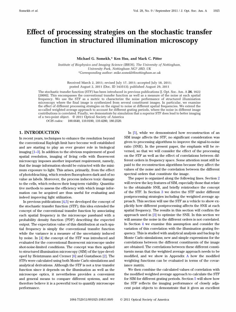
The effect of the SIM processing is depicted in Fig. 1for both cylindrical (one-dimensional) and spherical (two-dimensional) imaging systems. For the cylindrical case,Fig. 1(a) shows the situation that is obtained when the gratingfrequency mg is the maximum allowed by the aperture of theobjective, and Fig. 1(b) shows the case where mg is less thanthe maximum value of two normalized units of spatial fre-quency units, NAλ , where λ is the wavelength and NA is the nu-merical aperture of the microscope. Note that, throughout thispaper, we will assume, for simplicity, that the excitation andemission wavelengths are the same. Figure 1(c) shows thecase of the spherical system (an axially symmetric lens withuniform illumination) where it is necessary to project the grat-ing over a range of azimuthal angles in order to get good cov-erage of spatial frequency space; this issue is discussed inseveral publications [8]. For the case depicted in Fig. 1(c),three azimuthal angles at 0°, 60°, and 120° are used, wherethe shaded region represents the spatial frequencies coveredby SIM. Figure 1(d) shows how the recovered spatial fre-quencies from the carrier and the sidebands of the cylindricalsystem add to form a composite image corresponding to a mi-croscope of twice the NA. In this paper we will be concernedwith the noise carried by each of the spatial frequency ordersin the final image as well as the effect of combining the dif-ferent contributions in the image. For instance, in Fig. 1(a) wesee that, at spatial frequencym, both the carrier and the uppersideband carry information, whereas in Fig. 1(b) the carrier,upper sideband, and lower sideband all carry information,albeit to very different extents. Throughout this paper the cy-lindrical system will be used to develop the arguments sincethe spherical system is generally an extension of this case,although spherical imaging results will be presented whereappropriate.

As mentioned in Section 1, the concept of the STF associ-ates a PDF to each spatial frequency. For a conventionalfluorescent microscope, we have shown that the STF can be

m g =2

m g<2

-4

0-2 +2+4

Carrier

Upper sidebandLower sideband

m

0-2 +2

Carrier

Upper sidebandLower sideband

m

0 0

60

60

120

120

−4 −3 −2 −1 0 1 2 3 40

0.1

0.2

0.3

0.4

0.5

0.6

0.7

0.8

0.9

1

Spatial frequency, NA/wavelength

Tra

nsf

er f

un

ctio

n

(a)

(b)

(c)

(d)

Fig. 1. Relative position of spectral orders in SIM. (a) Position ofspectral orders in cylindrical SIM, for maximum grating frequency,mg ¼ 2. (b) Position of spectral orders in cylindrical SIM, for gratingfrequency, mg < 2. (c) Arrangement of spectral orders in sphericalSIM with three azimuthal projections for mg ¼ 2. The angles of theazimuthal projections are 0°, 60°, and 120°, respectively, and theshaded region represents the spatial frequency coverage. The solidblack circle represents the aperture of a conventional fluorescent mi-croscope with radius of two spatial frequency units, whereas thedashed circle has radius of four spatial frequency units. (d) Summationof spectral orders to recover extended transfer function for mg ¼ 2.Sideband weighting is half of carrier weighting.

1926 J. Opt. Soc. Am. A / Vol. 28, No. 9 / September 2011 Somekh et al.

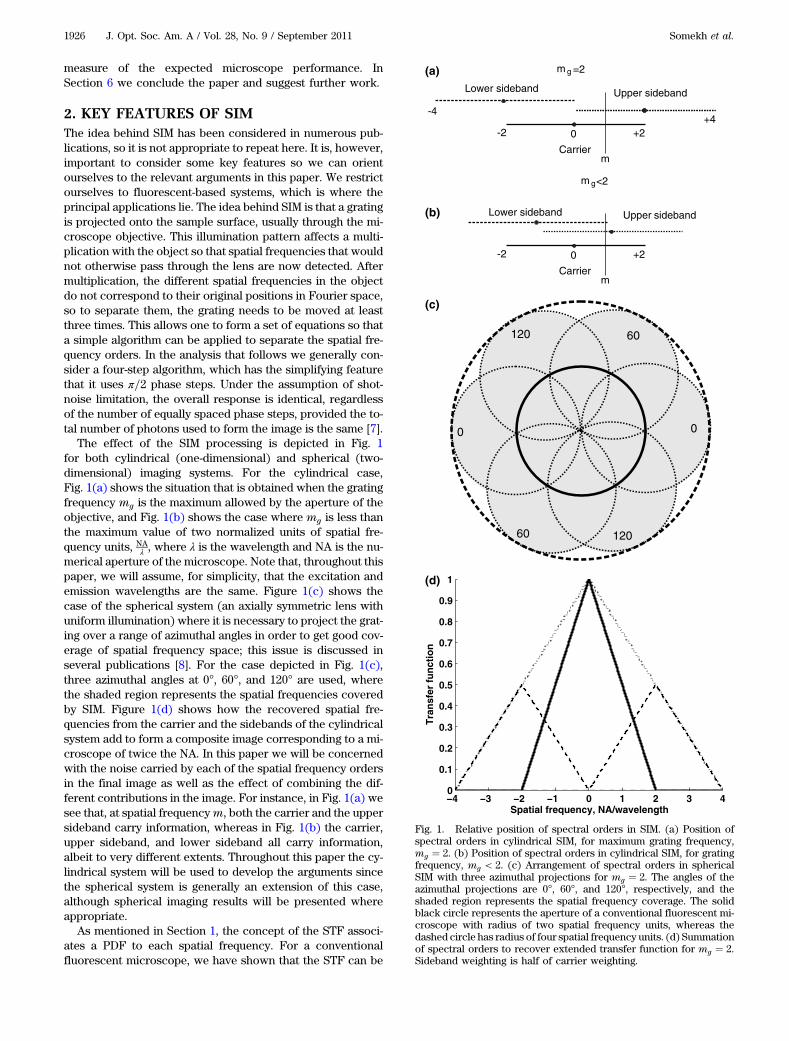
evaluated analytically or by Monte Carlo simulations [4]. Theanalytical approach involves derivation of the characteristicfunction for the even and odd parts of the transform and pro-vides compact expressions for the STF, which are confirmedby the Monte Carlo simulations. The derivation of the STF wasextended to SIM in [5]. For the SIM system, the processrequires that the effect of each of the constituent imagesbe incorporated. For both conventional fluorescence andSIM under shot-noise-limited condition, the form of the STFclearly depends on both the optical system and the numberof photons used to form the image. Figure 2 shows the normal-ized SNR, mean divided by standard deviation, μffiffiffiffi

σ2p of the cy-

lindrical imaging system for each type of microscope for atotal illumination corresponding to a single detected photonin the image. Note in previous publications [4,5], we used

the SNR defined as μ2σ2, which gives the SNR in terms of de-

tected electrical signal rather than optical power. Since weonly consider shot noise, the value of the SNR is simply ob-tained by multiplying the values obtained from Fig. 2 by thesquare root of the number of photons in the image, N . We con-cluded that, for the conventional microscope, the SNR is given

by SNR ¼ ffiffiffiffiN

pcðmÞ, where cðmÞ is the transfer function as a

function of spatial frequency, m. As expected the signal ex-tends to higher spatial frequencies for the SIM system, butthe noise variance is greater by a factor of 3 because thereis a similar noise contribution from each of the sidebands giv-

ing SNR ¼ffiffiffiN3

q½cðm2 Þ�. Them=2 in the argument for the transfer

function represents the fact that its support is twice as large.In Section 3 we will show that, in a practical SIM system, thereis a considerable amount of additional information, as well asfiltering, that allows one to make far more efficient use of theavailable photons, thus obtaining a far better SNR than indi-cated by the expression above.

3. SIM STF WITH MAXIMUM GRATINGFREQUENCYWe now examine the different processing strategies for SIMunder the assumption that the noise in the sidebands is uncor-related with that in the carrier. In Section 4 we show that this

assumption is valid when the grating is at the maximum spatialfrequency as shown in Fig. 1(a). We also show what happenswhen this condition is relaxed so that we have situation akinto Fig. 1(b), and we will demonstrate how this modifies therecovered SNR.

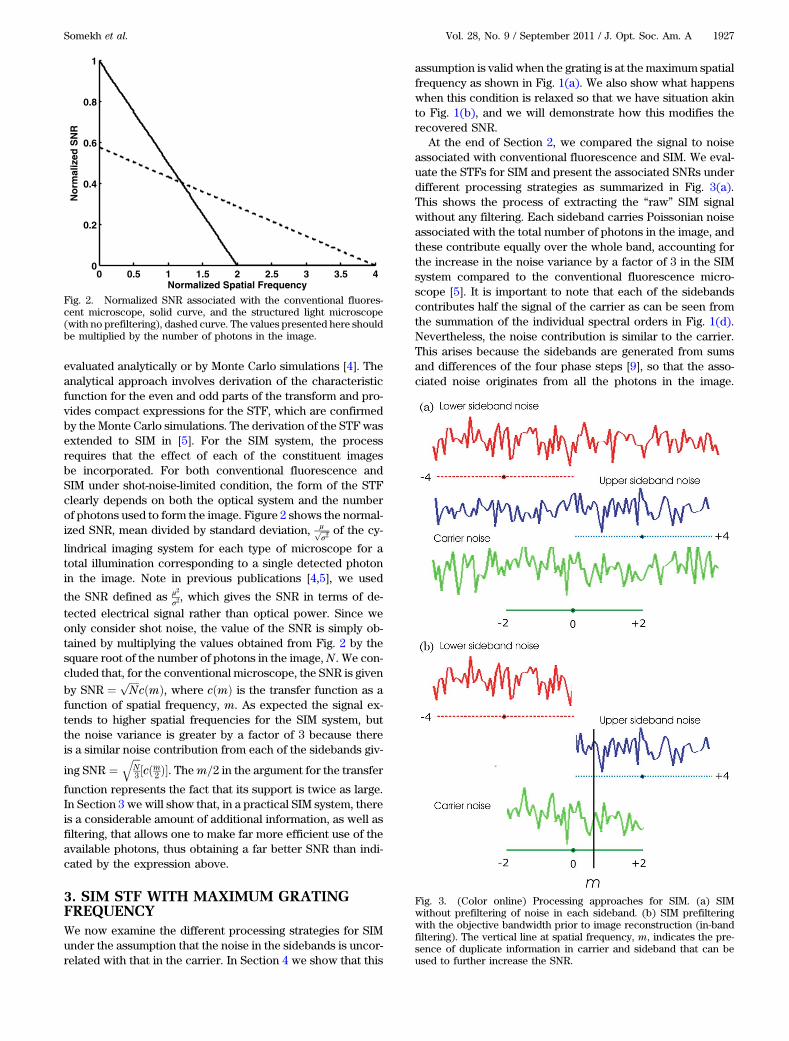
At the end of Section 2, we compared the signal to noiseassociated with conventional fluorescence and SIM. We eval-uate the STFs for SIM and present the associated SNRs underdifferent processing strategies as summarized in Fig. 3(a).This shows the process of extracting the “raw” SIM signalwithout any filtering. Each sideband carries Poissonian noiseassociated with the total number of photons in the image, andthese contribute equally over the whole band, accounting forthe increase in the noise variance by a factor of 3 in the SIMsystem compared to the conventional fluorescence micro-scope [5]. It is important to note that each of the sidebandscontributes half the signal of the carrier as can be seen fromthe summation of the individual spectral orders in Fig. 1(d).Nevertheless, the noise contribution is similar to the carrier.This arises because the sidebands are generated from sumsand differences of the four phase steps [9], so that the asso-ciated noise originates from all the photons in the image.

0 0.5 1 1.5 2 2.5 3 3.5 40

0.2

0.4

0.6

0.8

1

Normalized Spatial Frequency

No

rmal

ized

SN

R

Fig. 2. Normalized SNR associated with the conventional fluores-cent microscope, solid curve, and the structured light microscope(with no prefiltering), dashed curve. The values presented here shouldbe multiplied by the number of photons in the image.

Fig. 3. (Color online) Processing approaches for SIM. (a) SIMwithout prefiltering of noise in each sideband. (b) SIM prefilteringwith the objective bandwidth prior to image reconstruction (in-bandfiltering). The vertical line at spatial frequency, m, indicates the pre-sence of duplicate information in carrier and sideband that can beused to further increase the SNR.


As far as signal is concerned, the SIM processing is equivalentto generating displaced versions of the carrier transfer func-tion, while the noise behavior depends on the SIM processing.We will return to this theme in Section 4, where we considercorrelations between the carrier and sidebands and show thatSIM processing again ensures that the correlations are not thesame as simply displacing the carrier to form the sideband.Clearly, the processing depicted in Fig. 3(a), although instruc-tive, allows noise into the system, which can be readily elimi-nated without loss of signal. Filtering the signals in thepassband of the objective NA should lead to a significant im-provement. The process is depicted graphically in Fig. 3(b),where noise that is not associated with any signal is elimi-nated. We will refer to this as in-band filtering. The final stageof processing as used by Heintzmann [3] is to acknowledge,effectively, that the signals in the sidebands and carriers, ifthey are not perfectly correlated, each carry some indepen-dent sample information and can be combined to optimize theoverall signal to noise. The vertical line at spatial frequencymin Fig. 3(b) reminds us that both carrier and sideband containinformation at this spatial frequency.

A. Calculation of STFs Using Monte Carlo SimulationThe STFs may be evaluated using Monte Carlo simulations.The procedure is explained briefly below. There are fourphase steps in the image with a total of N photons given by

illnðxÞ ¼N4

�1þ cos

�2πmgxþ ðn − 1Þπ

2

��; ð1Þ

where the subscript n refers to the number of the phase step,mg is the grating frequency in units of NA

λ , and x is the spatialposition in units of λ

NA. Since the point object is located at theorigin, we can see that ill1ð0Þ ¼ N=2, ill2ð0Þ ¼ N=4, ill3ð0Þ ¼ 0,and ill4ð0Þ ¼ N=4. Each phase step then produces an impulseresponse with expectation number given by illnð0Þ. This is seg-mented into small regions that are a small fraction of λ

NA. Theexpectation value for this small region is then calculated, anda random Poisson number generator is used to produce a spe-cific value from the distribution. This can be used to calculatethe noisy impulse response for each phase step, which is Four-ier transformed and filtered to the bandwidth appropriate forthe reconstruction procedure used. The impulse response forthe carrier and sidebands is given by Eq. (2) below:

icarrierðmÞ ¼ i1ðmÞ þ i2ðmÞ þ i4ðmÞ; ð2aÞ

iupperðm −mgÞ ¼ i1ðm −mgÞ þ ji2ðm −mgÞ− ji4ðm −mgÞ; ð2bÞ

ilowerðmþmgÞ ¼ i1ðmþmgÞ − ji2ðmþmgÞþ ji4ðmþmgÞ; ð2cÞ

where the caret denotes the Fourier transform, and the thirdphase step is omitted as its value is zero at the origin.

The calculations were repeated 106 times to allow accurateevaluation of the means and variances of the different spectralorders.

The signals were then added without filtering (raw SIM),filtered to the objective bandwidth and added (in-band SIM)

or filtered and combined with a weighted average. In order tocombine the signals from carrier and sideband(s) with theweighted average, we determine a so-called goal transfer func-tion, Hgoal [10], that is the desired transfer function after pro-cessing. In this case we used, as is common in practice, thetransfer function of a notional conventional microscope(NCM) with twice the NA. A “conventional” microscope withthis transfer function may, of course, not be physically realiz-able as it could entail detection of nonpropagating modes.

The analysis in Appendix A derives the weightings for thedifferent contributions to maximize the SNR for a given goaltransfer function. These results are generalized to include cor-relations between the different contributions; setting these tozero in Eqs. (A5) and (A6) allows us to apply the weightedaverage for uncorrelated contributions.

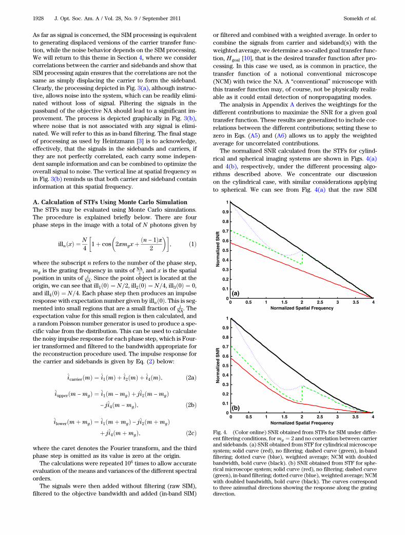
The normalized SNR calculated from the STFs for cylind-rical and spherical imaging systems are shown in Figs. 4(a)and 4(b), respectively, under the different processing algo-rithms described above. We concentrate our discussionon the cylindrical case, with similar considerations applyingto spherical. We can see from Fig. 4(a) that the raw SIM

0 0.5 1 1.5 2 2.5 3 3.5 40

0.1

0.2

0.3

0.4

0.5

0.6

0.7

0.8

0.9

1


0 0.5 1 1.5 2 2.5 3 3.5 40

0.1

0.2

0.3

0.4

0.5

0.6

0.7

0.8

0.9

1


No

rmal

ized

SN

RN

orm

aliz

ed S

NR

(a)

(b)

Fig. 4. (Color online) SNR obtained from STFs for SIM under differ-ent filtering conditions, formg ¼ 2 and no correlation between carrierand sidebands. (a) SNR obtained from STF for cylindrical microscopesystem; solid curve (red), no filtering; dashed curve (green), in-bandfiltering; dotted curve (blue), weighted average; NCM with doubledbandwidth, bold curve (black). (b) SNR obtained from STF for sphe-rical microscope system; solid curve (red), no filtering; dashed curve(green), in-band filtering; dotted curve (blue), weighted average; NCMwith doubled bandwidth, bold curve (black). The curves correspondto three azimuthal directions showing the response along the gratingdirection.


algorithm gives an SNR equal to 1=p3 that of a conventional

microscope system at m ¼ 0, as discussed above. A slightlybetter situation arises for the in-band filtering case [greendashed, Fig. 4(a)] as depicted in Fig. 3(b) where we againadd carrier and sidebands but filter out areas where no signalis present. We can see that effectively we have an SNR equalto 1=

p2 that of the conventional microscope; this can be seen

from the fact that there are now two noise contributions as wemove to a spatial frequency infinitesimally greater than zero.Abovem ¼ 2 the signal to noise suddenly improves by a factorof

p2 because the noise from the carrier is removed at this

point; slightly below mg ¼ 2 the carrier contributes virtuallyno signal but still adds noise to the system. The preferredarrangement is the weighted average approach [blue dotted,Fig. 4(a)] where the carriers and sideband are incorporatedaccording to their SNR. At low spatial frequencies the side-bands make very little contribution to the signal so that theweighted average essentially “switches” them off so the signalto noise is the same as the NCM. The weighted averagealgorithm shows very considerable benefits as the spatial fre-quency approaches 2 because here the sideband has a muchbetter signal to noise than the carrier. For values ofm > 2, theweighted average and in-band filtering give the same resultbecause there is only a single contribution to the signal. Itis worth pointing out that, at m ¼ 4=3, both in-band filteringand the weighted average give the same result. This is becauseat this spatial frequency the SNR for carrier and sideband arethe same, so each contribution is equally weighted, equivalentto a simple summation. In summary, weighted averaging givesthe superior SNR to the other approaches. It is worth compar-ing these SIM curves with those pertaining to the NCM whereeven the weighted average process is inferior to the NCM be-cause the necessary processing induces additional noise in thepassband. Note that, form > 2, in-band and weighted averageare identical to the NCM because the carrier contributionfollows the extended bandwidth transfer function exactly[see Fig. 1(d)].

The spherical plots shown in Fig. 4(b) depend on thenumber of azimuthal directions used to produce the recon-struction. First, we should note that, for a finite number ofazimuthal projections, the exact transfer function dependson the direction relative to the grating projections. For threedifferent projection directions, the response can be regardedto a reasonable, practical approximation as isotropic with thecut-off frequency along the grating projections being equal tofour normalized units. The lowest cut-off frequency, which oc-curs at 30° from this direction, is 2

p3. The plots presented in

Fig. 4(b), which use three grating projection directions, showsections along a grating projection direction. The noise factorof

p3 still applies for the unfiltered response since each azi-

muthal projection carries noise associated with the total num-ber of photons in the image divided by the number azimuthalgrating projections, and since each azimuthal projection re-presents an independent noise source, the noise from theseprojections is additive. We see again that the weighted aver-age gives the best transfer function, as expected, and that it isidentical to the in-band filtering abovem ¼ 2. As expected theNCM has better performance than SIM, and indeed the dif-ference is, as we may expect, even greater than it is in thecylindrical case.

4. SIM STF WITH CORRELATIONSBETWEEN CARRIER AND SIDEBANDSIn Section 3 we worked under the presumption that there is nocorrelation between the sidebands, an assumption made inprevious work [3]. We now examine the conditions that deter-mine the correlation between sidebands and the effects on theSTF. We consider this issue analytically; however, the analy-tical approach yields the correlation between the carrier andboth of the sidebands. To resolve this, we use Monte Carlosimulations to obtain the correlation with each sidebandand also the correlation between the sidebands. We considerthe cylindrical case where a relatively simple expressionfor the correlation between the carrier and the sidebands isobtained.

A. Analytical Derivation of Correlation between Carrierand SidebandsIn order to determine the correlations between carriers andsidebands, our approach is to calculate the joint PDF forthe output between carrier and sidebands. We follow a similarapproach to that developed in [5,9]. The idea is to calculate thejoint PDF for the Poissonian noise process when the signal ismultiplied by two different deterministic functions. The basicmethod was derived for a single variable in [9] and extendedto a joint PDF in [5]. We consider a distribution in the imagegiven by iðxÞwhich is subject to Poissonian noise. Wemultiplyeach function by deterministic functions f aðxÞ and f bðxÞ; therole of these functions will be apparent later. We show in [9]that the characteristic function is given by

Aðϕ;ψÞ ¼ expZR

iðxÞfexp½j2πðf aðxÞϕþ f bðxÞψÞ� − 1gdx; ð3Þ

where ϕ and ψ are the transform variables associated with thecharacteristic function and R is the region of integration overwhich we wish to determine the PDF; in this case these limitswill be from −∞ to þ∞. The joint PDF may be recovered byinverse Fourier transforming Aðϕ;ψÞ, but in our case this isnot necessary as we can recover the correlation coefficientsfrom the characteristic function directly.

We now introduce the terms in the integrand in terms of N ,the total number of photons in the image, and HðxÞ, the inten-sity impulse response of the microscope:

i1ðxÞ ¼N2HðxÞ; i2ðxÞ ¼ i4ðxÞ ¼

N4HðxÞ: ð4Þ

The factors of 1=2 and 1=4 arise from the illumination pat-tern given by Eq. (1).

Two additional issues arise at this point; in order to keepthe argument in the integrand of Eq. (3) real, rather than cal-culating a Fourier transform directly, we use a cosine and asine transform. Second, since Eq. (3) operates in the spatialdomain, we use Eq. (5) below to perform the reconstruction.

This algorithm is given by [9]

isðxÞ ¼ ½1þ 2 cosð2πmgxÞ�i1ðxÞ þ ½1 − 2 sinð2πmgxÞ�i2ðxÞþ ½1þ 2 sinð2πmgxÞ�i4ðxÞ; ð5Þ

where isðxÞ is the recovered SIM signal. The carrier is givenby the constant factors, and the sidebands are given by the


trigonometric factors. The characteristic functions for eachterm in Eq. (3) are multiplied together to obtain the overallcharacteristic function. Treating the odd and even parts ofthe Fourier transform separately, we obtain

Aeðϕ;ψÞ ¼Yn

Aenðϕ;ψÞ; ð6aÞ

Aoðϕ;ψÞ ¼Yn

Aonðϕ;ψÞ: ð6bÞ

For the carrier term we have

f ae1ðxÞf ao1ðxÞ

�¼

� cos 2πmx

sin 2πmx;


�¼

� cos 2πmx

sin 2πmx;


�¼

� cos 2πmx

sin 2πmx; ð7Þ

and for the sidebands

f be1ðxÞf bo1ðxÞ

�¼ 2 cos 2πmgx

� cos 2πmx

sin 2πmx;


�¼ −2 sin 2πmgx

� cos 2πmx

sin 2πmx;


�¼ 2 sin 2πmgx

� cos 2πmx

sin 2πmx: ð8Þ

To obtain our result, we make one further approximation: thatN is large. This was discussed in detail in [5], where weshowed that for N to be treated as large a value of 20 is suffi-cient. The large N approximation allows us to expand the ar-gument to the second order to obtain an analytical expressionfor Aðϕ;ψÞ:

Aðϕ;ψÞ ¼ exp�Z

R

NHðxÞf2πj½f aðxÞϕþ f bðxÞψ � − 2π2½f 2aðxÞϕ2

þ f 2bðxÞψ2 þ 2f aðxÞf bðxÞϕψ �gdx�: ð9Þ

After expansion and substitution with Eq. (8), we obtainseveral terms of the form

Z∞−∞

HðxÞ�cosðkmþ lmgÞxsinðkmþ lmgÞx dx ¼

�cðkmþ lmgÞ

0; ð10Þ

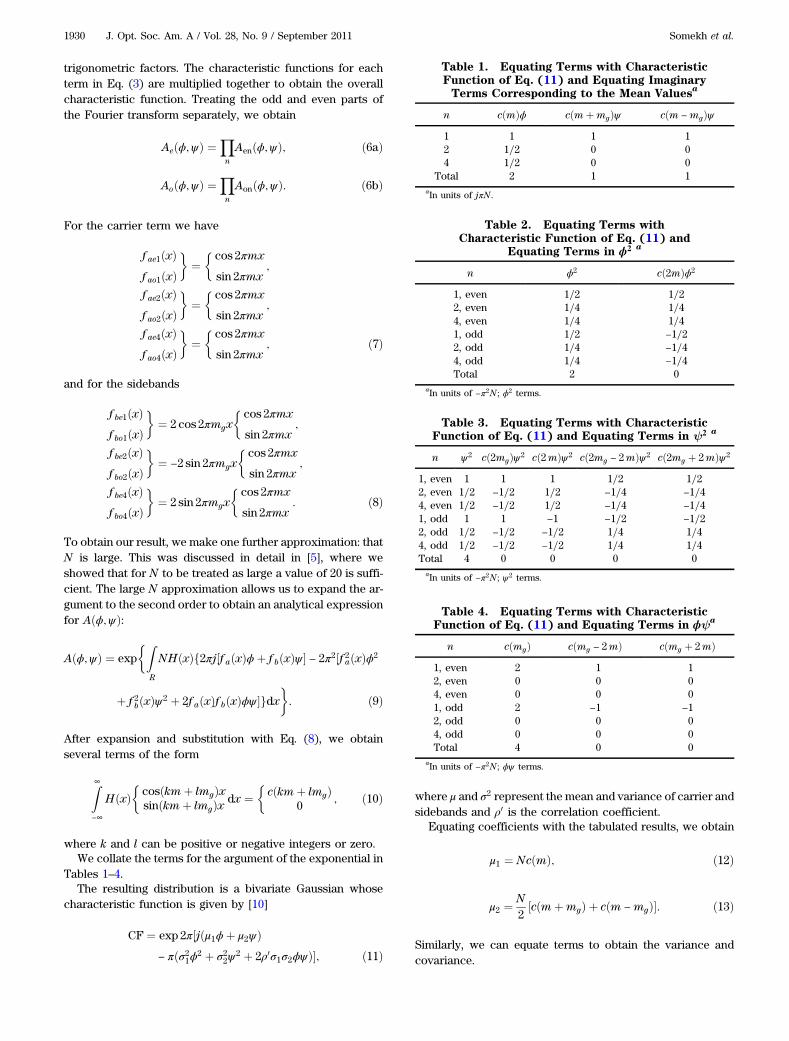
where k and l can be positive or negative integers or zero.We collate the terms for the argument of the exponential in

Tables 1–4.The resulting distribution is a bivariate Gaussian whose

characteristic function is given by [10]

CF ¼ exp 2π½jðμ1ϕþ μ2ψÞ− πðσ21ϕ2 þ σ22ψ2 þ 2ρ0σ1σ2ϕψÞ�; ð11Þ

where μ and σ2 represent the mean and variance of carrier andsidebands and ρ0 is the correlation coefficient.

Equating coefficients with the tabulated results, we obtain

μ1 ¼ NcðmÞ; ð12Þ

μ2 ¼N2½cðmþmgÞ þ cðm −mgÞ�: ð13Þ

Similarly, we can equate terms to obtain the variance andcovariance.

Table 1. Equating Terms with Characteristic

Function of Eq. (11) and Equating Imaginary

Terms Corresponding to the Mean Valuesa

n cðmÞϕ cðmþmgÞψ cðm −mgÞψ1 1 1 12 1=2 0 04 1=2 0 0

Total 2 1 1aIn units of jπN .

Table 2. Equating Terms with

Characteristic Function of Eq. (11) and

Equating Terms in ϕ2 a

n ϕ2 cð2mÞϕ2

1, even 1=2 1=22, even 1=4 1=44, even 1=4 1=41, odd 1=2 −1=22, odd 1=4 −1=44, odd 1=4 −1=4Total 2 0

aIn units of −π2N ; ϕ2 terms.


Function of Eq. (11) and Equating Terms in ψ2 a

n ψ2 cð2mgÞψ2 cð2mÞψ2 cð2mg − 2mÞψ2 cð2mg þ 2mÞψ2

1, even 1 1 1 1=2 1=22, even 1=2 −1=2 1=2 −1=4 −1=44, even 1=2 −1=2 1=2 −1=4 −1=41, odd 1 1 −1 −1=2 −1=22, odd 1=2 −1=2 −1=2 1=4 1=44, odd 1=2 −1=2 −1=2 1=4 1=4Total 4 0 0 0 0

aIn units of −π2N ; ψ2 terms.


Function of Eq. (11) and Equating Terms in ϕψa

n cðmgÞ cðmg − 2mÞ cðmg þ 2mÞ1, even 2 1 12, even 0 0 04, even 0 0 01, odd 2 −1 −12, odd 0 0 04, odd 0 0 0Total 4 0 0

aIn units of −π2N ; ϕψ terms.


This leads to

σ21 ¼ N; σ22 ¼ 2N: ð14Þ

Using these values and equating to the sum of the real andimaginary part of ϕψ gives the covariance, cov, from whichwe obtain the expression for the correlation between carrierand sidebands:

cov ¼ NcðmgÞ; ð15Þ

ρ0 ¼ covffiffiffiffiffiffiffiffiffiσ21σ22

q ¼ 1ffiffiffi2

p cðmgÞ: ð16Þ

Equation (16) gives the correlation between the carrierand both of the sidebands. By symmetry we expectcovðcarrier; upper sidebandÞ ¼ covðcarrier; lower sidebandÞ,so we obtain a value for the covariance of 1=2 the value givenin Eq. (15) for the covariance between the carrier and a singlesideband. Since we are now concerned with the variance ofonly one sideband, the variance is reduced by a factor of 2. Wetherefore obtain an expression for the correlation between thecarrier and a single sideband:

ρ ¼ NcðmgÞ2

ffiffiffiffiN

p ffiffiffiffiN

p ¼ cðmgÞ2

: ð17Þ

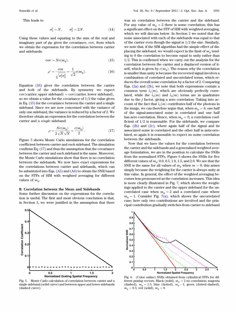
Figure 5 shows Monte Carlo simulations for the correlationcoefficient between carrier and each sideband. The simulationconfirms Eq. (17) and thus the assumption that the covariancebetween the carrier and each sideband is the same. Moreover,the Monte Carlo simulations show that there is no correlationbetween the sidebands. We now have exact expressions forthe correlations between carrier and sidebands, which canbe substituted into Eqs. (A5) and (A6) to obtain the SNR basedon the STFs of SIM with weighted averaging for differentvalues of mg.

B. Correlation between the Mean and SidebandsSome further discussion on the expressions for the correla-tion is useful. The first and most obvious conclusion is that,in Section 3, we were justified in the assumption that there

was no correlation between the carrier and the sideband.For any value of mg < 2 there is some correlation; this hasa significant effect on the STF of SIMwith weighted averaging,which we will discuss below. In Section 2 we noted that thenoise associated with each of the sidebands was equal to thatof the carrier even though the signal is 1=2 the size. Similarly,we note that, if the SIM algorithm had the simple effect of dis-placing the sideband, we would expect in the limit ofmg tend-ing to 0 the correlation to become equal to unity rather than1=2. This is confirmed when we carry out the analysis for thecorrelation between the carrier and a displaced version of it-self, which is given by cðmgÞ. The reason why the correlationis smaller than unity is because the recovered signal involves acombination of correlated and uncorrelated terms, which re-duces the overall noise correlation by a factor of 2. ComparingEqs. (2a) and (2b), we note that both expressions contain acommon term i1ðmÞ, which are obviously perfectly corre-lated, while the i2ðmÞ and i4ðmÞ terms are in quadraturedue to the j factor, giving a zero correlation. Taking into ac-count of the fact that i1ðmÞ contributes half of the photons inthe image, we can therefore argue that, whenmg ¼ 0, one halfof the signal-associated noise is correlated and one halfhas zero correlation. Hence, when mg ¼ 0, a correlation coef-ficient of 1=2 is reasonable. For the sidebands, we compareEqs. (2b) and (2c), where again half of the signal and itsassociated noise is correlated and the other half is anticorre-lated, so again it is reasonable to expect no noise correlationbetween the sidebands.

Now that we have the values for the correlation betweenthe carrier and the sidebands and a generalized weighted aver-age formulation, we are in the position to calculate the SNRsfrom the normalized STFs. Figure 6 shows the SNRs for fivedifferent values ofmg: 0.0, 0.5, 1.0, 1.5, and 2.0. We see that theSNR is the same for all values of mg when m ¼ 0; this arisessimply because the weighting for the carrier is always unity atthis value. In general, the effect of the weighted averaging be-comes less pronounced as the correlation increases. This ideais more clearly illustrated in Fig. 7, which shows the weight-ings applied to the carrier and the upper sideband for the un-correlated case when mg ¼ 2 and a correlated case wheremg ¼ 1. Consider Fig. 7(a), which shows the uncorrelatedcase; here only two contributions are involved and the prin-cipal contribution gradually switches from carrier to sideband

0 0.5 1 1.5 2 2.5 3 3.5 40

0.1

0.2

0.3

0.4

0.5

0.6

0.7

0.8

0.9

1


No

rmal

ized

SN

R

Fig. 6. (Color online) SNRs obtained from cylindrical STFs for dif-ferent grating vectors. Black (solid), mg ¼ 2 no correlation; magenta(dashed), mg ¼ 1:5; blue (dotted), mg − 1; green (dotted–dashed),mg ¼ 0:5; red (solid), mg ¼ 0.

0 0.5 1 1.5 2

0

0.1

0.2

0.3

0.4

0.5

Normalized Grating Spatial Frequency

Co

rrel

atio

n C

oef

fici

ent

Fig. 5. Monte Carlo calculation of correlation between carrier and asingle sideband (solid curve) and between upper and lower sidebands(dashed curve).


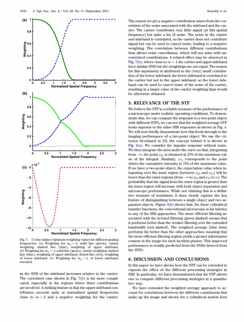
as the SNR of the sideband increases relative to the carrier.The correlated case shown in Fig. 7(b) is far more compli-cated, especially in the regions where three contributionsare involved. A striking feature is that the upper sideband con-tribution exceeds unity at normalized spatial frequenciesclose to m ¼ 2 and a negative weighting for the carrier.

The reason we get a negative contribution arises from the cor-relation of the noise associated with the sideband and the car-rier. The carrier contributes very little signal (at this spatialfrequency) but quite a lot of noise. The noise in the carrierand sideband is correlated, so the carrier does not contributesignal but can be used to cancel noise, leading to a negativeweighting. The correlation between different contributionsthus allows noise cancellation, which will not arise with un-correlated contributions. A related effect may be observed inFig. 7(b), where close tom ¼ 1 the carrier and upper sidebandhave similar SNR but the weightings are not equal. The reasonfor this asymmetry is attributed to the (very) small contribu-tion of the lower sideband; the lower sideband is correlated tothe carrier but not to the upper sideband, so the lower side-band can be used to cancel some of the noise of the carrier,resulting in a larger value of the carrier weighting than wouldbe otherwise obtained.

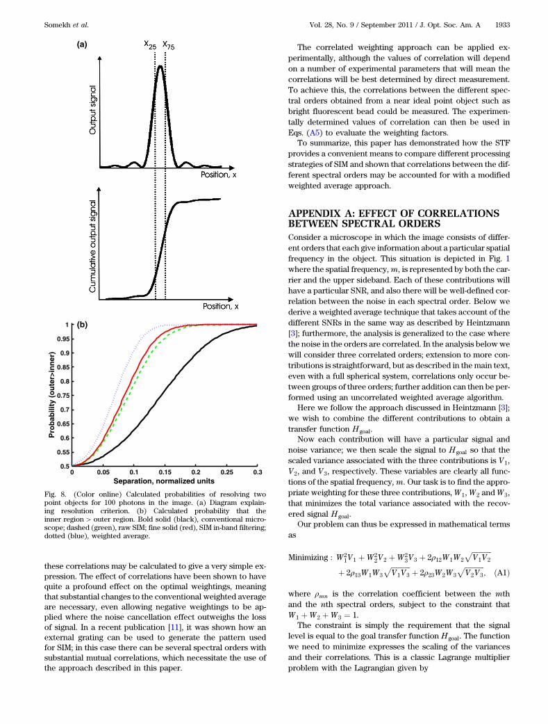
5. RELEVANCE OF THE STFWe believe the STF is a reliable measure of the performance ofa microscope under realistic operating conditions. To demon-strate this, we can compare the response to a two-point objectwith different STFs; we can see that the weighted average STFlooks superior to the other SIM responses as shown in Fig. 4.We will now briefly demonstrate how this feeds through to theimaging performance of a two-point object. We use the cri-terion developed in [9]; the concept behind it is shown inFig. 8(a). We consider the impulse response without noise.We then integrate the area under the curve so that, integratingfrom −∞, the point x25 is obtained at 25% of the maximum val-ue of the integral. Similarly, x75 corresponds to the pointwhere the cumulative intensity is 75% of the maximum value.If we have a two-point object, the expectation value when in-tegrating over the inner region (between x25 and x75) will belower than the outer regions (from −∞ to x25 and x75 to∞). Theprobability that the signal from the outer region is greater thanthe inner region will increase with both object separation andmicroscope performance. While not claiming this is a defini-tive measure of resolution, it does clearly capture the keyfeature of distinguishing between a single object and two se-parated objects. Figure 8(b) shows that, for these cylindricaltransfer functions, the conventional microscope is far inferiorto any of the SIM approaches. The more efficient filtering as-sociated with the in-band filtering (green dashed) means thatit performs better than the weaker filtering over the extendedbandwidth (red dashed). The weighted average (blue dots)performs far better than the other approaches, meaning thatthe more efficient filtering regime yields a greater informationcontent in the image for each incident photon. This improvedperformance is readily predicted from the SNRs derived fromthe STFs.

6. DISCUSSION AND CONCLUSIONSIn this paper we have shown how the STF can be extended toexpress the effect of the different processing strategies inSIM. In particular, we have demonstrated that the STF allowsone to compare different processing strategies in a quantita-tive way.

We have extended the weighted average approach to ac-count for correlations between the different constituents thatmake up the image and shown for a cylindrical system how


Wei

gh

tin

g

0 0.5 1 1.5 2 2.5 3 3.5 40

0.2

0.4

0.6

0.8

1

0 0.5 1 1.5 2 2.5 3

0

0.2

0.4

0.6

0.8

1


Wei

gh

tin

g

0 0.5 1 1.5 2 2.5 3−12

−10

−8

−6

−4

−2

0x 10

−3


Wei

gh

tin

g(a)

(b)

(c)

Fig. 7. (Color online) Optimumweighting values for different gratingfrequencies. (a) Weighting for mg ¼ 2; solid line (green), carrierweighting; dashed line (blue), weighting of upper sideband.(b) Weighting formg ¼ 1; solid line (green), carrier weighting; dashedline (blue), weighting of upper sideband; dotted line (red), weightingof lower sideband. (c) Weighting for mg ¼ 1, of lower sideband,rescaled.


these correlations may be calculated to give a very simple ex-pression. The effect of correlations have been shown to havequite a profound effect on the optimal weightings, meaningthat substantial changes to the conventional weighted averageare necessary, even allowing negative weightings to be ap-plied where the noise cancellation effect outweighs the lossof signal. In a recent publication [11], it was shown how anexternal grating can be used to generate the pattern usedfor SIM; in this case there can be several spectral orders withsubstantial mutual correlations, which necessitate the use ofthe approach described in this paper.

The correlated weighting approach can be applied ex-perimentally, although the values of correlation will dependon a number of experimental parameters that will mean thecorrelations will be best determined by direct measurement.To achieve this, the correlations between the different spec-tral orders obtained from a near ideal point object such asbright fluorescent bead could be measured. The experimen-tally determined values of correlation can then be used inEqs. (A5) to evaluate the weighting factors.

To summarize, this paper has demonstrated how the STFprovides a convenient means to compare different processingstrategies of SIM and shown that correlations between the dif-ferent spectral orders may be accounted for with a modifiedweighted average approach.

APPENDIX A: EFFECT OF CORRELATIONSBETWEEN SPECTRAL ORDERSConsider a microscope in which the image consists of differ-ent orders that each give information about a particular spatialfrequency in the object. This situation is depicted in Fig. 1where the spatial frequency,m, is represented by both the car-rier and the upper sideband. Each of these contributions willhave a particular SNR, and also there will be well-defined cor-relation between the noise in each spectral order. Below wederive a weighted average technique that takes account of thedifferent SNRs in the same way as described by Heintzmann[3]; furthermore, the analysis is generalized to the case wherethe noise in the orders are correlated. In the analysis belowwewill consider three correlated orders; extension to more con-tributions is straightforward, but as described in the main text,even with a full spherical system, correlations only occur be-tween groups of three orders; further addition can then be per-formed using an uncorrelated weighted average algorithm.

Here we follow the approach discussed in Heintzmann [3];we wish to combine the different contributions to obtain atransfer function Hgoal.

Now each contribution will have a particular signal andnoise variance; we then scale the signal to Hgoal so that thescaled variance associated with the three contributions is V1,V2, and V3, respectively. These variables are clearly all func-tions of the spatial frequency,m. Our task is to find the appro-priate weighting for these three contributions,W1,W2 andW3,that minimizes the total variance associated with the recov-ered signal Hgoal.

Our problem can thus be expressed in mathematical termsas

Minimizing : W21V1 þW2

2V2 þW23V3 þ 2ρ12W1W2

ffiffiffiffiffiffiffiffiffiffiffiV1V2

pþ 2ρ13W1W3

ffiffiffiffiffiffiffiffiffiffiffiV 1V3

pþ 2ρ23W2W3


p; ðA1Þ

where ρmn is the correlation coefficient between the mthand the nth spectral orders, subject to the constraint thatW1 þW2 þW3 ¼ 1.

The constraint is simply the requirement that the signallevel is equal to the goal transfer function Hgoal. The functionwe need to minimize expresses the scaling of the variancesand their correlations. This is a classic Lagrange multiplierproblem with the Lagrangian given by

0 0.05 0.1 0.15 0.2 0.25 0.30.5

0.55

0.6

0.65

0.7

0.75

0.8

0.85

0.9

0.95

1

Separation, normalized units

Pro

bab

ility

(o

ute

r>in

ner

)(a)

(b)

Fig. 8. (Color online) Calculated probabilities of resolving twopoint objects for 100 photons in the image. (a) Diagram explain-ing resolution criterion. (b) Calculated probability that theinner region > outer region. Bold solid (black), conventional micro-scope; dashed (green), raw SIM; fine solid (red), SIM in-band filtering;dotted (blue), weighted average.


F ¼ W21V1 þW2

2V2 þW23V3 þ 2ρ12W1W2


pþ 2ρ13W1W3


pþ 2ρ23W2W3


pþ λðW1 þW2 þW3 − 1Þ: ðA2Þ

Differentiating with respect to the weightings and equating tozero, we obtain

∂F∂W1

¼ 2W1V1þ2ρ12W2

ffiffiffiffiffiffiffiffiffiffiffiV1V 2

pþ2ρ13W3


pþλ¼ 0;

∂F∂W2

¼ 2W2V2þ2ρ12W1


pþ2ρ23W3


pþλ¼ 0;

∂F∂W3

¼ 2W3V3þ2ρ13W1


pþ2ρ23W2


pþλ¼ 0: ðA3Þ

This is equivalent to

½cov�"W1

W2

W3

#¼ −

λ2

" 111

#; ðA4Þ

where ½cov� is the covariance matrix.Solving these simultaneous equations and applying the con-

straint, we obtain

W1 ¼α1

α1 þ α2 þ α3; ðA5aÞ

W2 ¼α2

α1 þ α2 þ α3; ðA5bÞ

W3 ¼α3

α1 þ α2 þ α3; ðA5cÞ

where

α1 ¼ V2V 3ð1 − ρ223Þ þ V3


pðρ13ρ23 − ρ12Þ

þ V2


pðρ12ρ23 − ρ13Þ;

α2 ¼ V1V 3ð1 − ρ213Þ þ V3



þ V1


pðρ12ρ13 − ρ23Þ;

α3 ¼ V1V 2ð1 − ρ212Þ þ V1



þ V2


pðρ12ρ23 − ρ13Þ:

For two contributions, these expressions simplify to

W1 ¼V2 − ρ


pV1 þ V2 − 2ρ


p ;

W2 ¼V1 − ρ


pV1 þ V2 − 2ρ


p ; ðA6Þ

where the subscripts for ρ have been dropped as they are re-dundant in this case.

We can see immediately that, when there is no correlation,the weightings reduce to the expressions used in Section 3 asexpected.

ACKNOWLEDGMENTSThe authors acknowledge the financial support of theEngineering and Physical Sciences Research Council(EPSRC) for a platform grant entitled “Strategies for OptimalBiological Imaging” that partially funded this work. K. Hsu ac-knowledges Nottingham University for supporting a Ph.D.studentship, and M. G. Somekh would like to thank ProfessorAaron Ho of the Chinese University of Hong Kong for kindlysupporting a sabbatical visit that provided the time tocomplete this work.

REFERENCES1. S. W. Hell, M. Schrader, and H. T. M. van der Voort, “Far-field

fluorescence microscopy with three-dimensional resolution inthe 100nm range,” J. Microsc. 187, 1–7 (1997).

2. M. G. L. Gustafsson, “Surpassing the lateral resolution limit by afactor of two using structured illumination microscopy,” J. Mi-crosc. 198, 82–87 (2000).

3. R. Heintzmann, “Saturated patterned excitation microscopywith two-dimensional excitation patterns,” Micron 34, 283–291(2003).

4. K. Hsu, M. G. Somekh, and M. C. Pitter, “Stochastic transferfunction: application to fluorescence microscopy,” J. Opt.Soc. Am. A 26, 1622–1629 (2009).

5. M. G. Somekh, K. Hsu, and M. C. Pitter, “Stochastic transferfunction for structured illumination microscopy,” J. Opt. Soc.Am. A 26, 1630–1637 (2009).

6. R. Heintzmann and C. Cremer, “Laterally modulated excitationmicroscopy: improvement of resolution by using a diffractiongrating,” Proc. SPIE 3568, 185–196 (1999).

7. K. Hsu, “Stochastic analysis of lateral resolution and signal-to-noise ratio in fluorescence microscopy: application to struc-tured illumination microscopy,” Ph.D. thesis (University ofNottingham, 2010).

8. E. Chung, D. Kim, Y. Cui, Y.-H. Kim, and P. T. C. So,“Two-dimensional standing wave total internal reflectionfluorescence microscopy: superresolution imaging of singlemolecular and biological specimens,” Biophys. J. 93, 1747–1757(2007).

9. M. G. Somekh, K. Hsu, andM. C. Pitter, “Resolution in structuredillumination microscopy: an analytical probabilistic approach,”J. Opt. Soc. Am. A 25, 1319–1329 (2008).

10. A. Papoulis, Probability Random Variables and StochasticProcesses (McGraw Hill, 1965), Chap. 7, p. 226.

11. C. W. See, C. J. Chuang, S. G. Liu, and M. G. Somekh, “Proximityprojection grating structured light illumination microscopy,”Appl. Opt. 49, 6570–6576 (2010).


Documents

Effect of processing strategies on the stochastic transfer function in structured illumination microscopy