Effect of Preconditioning on the Extreme Climate …iprc.soest.hawaii.edu/users/jimp/papers/iozm_idec.pdf · Effect of Preconditioning on the Extreme Climate Events in the Tropical

Effect of Preconditioning on the Extreme Climate Events in the Tropical Indian Ocean*H. ANNAMALAI AND J. POTEMRA

International Pacific Research Center, University of Hawaii at Manoa, Honolulu, Hawaii

R. MURTUGUDDE

ESSIC, University of Maryland, College Park, College Park, Maryland

J. P. MCCREARY

International Pacific Research Center, University of Hawaii at Manoa, Honolulu, Hawaii

(Manuscript received 12 March 2004, in final form 29 March 2005)

ABSTRACT

Sea surface temperature observations in the eastern equatorial Indian Ocean (EEIO) during the period1950–2003 indicate that Indian Ocean dipole/zonal mode (IODZM) events are strong in two decades,namely, the 1960s and 1990s. Atmospheric reanalysis products in conjunction with output from an oceanmodel are examined to investigate the possible reason for the occurrence of strong IODZM events in thesetwo decades. Specifically, the hypothesis that the mean thermocline in the EEIO is raised or lowereddepending on the phase of Pacific decadal variability (PDV), preconditioning the EEIO to favor strongeror weaker IODZM activity, is examined. Diagnostics reveal that the EEIO is preconditioned by thetraditional PDV signal (SVD1 of SST), deepening or shoaling the thermocline off south Java through itsinfluence on the Indonesian Throughflow (ITF; oceanic teleconnection), and by residual decadal variabilityin the western and central Pacific (SVD2 of SST) that changes the equatorial winds over the Indian Ocean(atmospheric teleconnection). Both effects produce a background state that is either favorable or unfavor-able for the thermocline–mixed layer interactions, and hence for the excitation of strong IODZM events.Collectively, SVD1 and SVD2 are referred to as PDV here.

This hypothesis is tested with a suite of ocean model experiments. First, two runs are carried out, forcedby climatological winds to which idealized easterly or westerly winds are added only over the equatorialIndian Ocean. As might be expected, in the easterly (westerly) run a shallower (deeper) thermocline isobtained over the EEIO. Then, observed winds from individual years are used to force the model. In theseruns, anomalously cool SST in the EEIO develops only during decades when the thermocline is anoma-lously shallow, allowing entrainment of colder waters into the mixed layer.

Since 1999 the PDV phase has changed, and consistent with this hypothesis the depth of the meanthermocline in the EEIO has been increasing. As a consequence, no IODZM developed during the El Niñoof 2002, and only a weak cooling event occurred during the summer of 2003. This hypothesis likely alsoexplains why some strong IODZM events occur in the absence of ENSO forcing, provided that PDV haspreconditioned the EEIO thermocline to be anomalously shallow.

1. Introduction

a. Background

Recent studies point toward the existence of a natu-ral mode of climate variability in the Indian Ocean,

known either as the Indian Ocean dipole/zonal mode(IODZM; Reverdin et al. 1986; Murtugudde et al.1998b; Saji et al. 1999; Webster et al. 1999; Behera etal. 1999; Murtugudde and Busalacchi 1999; Yu andRienecker 1999, 2000). As part of this mode, sea sur-face temperature (SST) in the eastern equatorial IndianOcean (EEIO; in the neighborhood of 10°S–0°, 90°–110°E) becomes anomalously cool during boreal sum-mer and fall, weakening the overlying precipitation; thischange in atmospheric heating forces an anticyclone inthe lower atmosphere over the southeastern IndianOcean as a Rossby wave response (e.g., Annamalai etal. 2003). The resulting winds increase upwelling offSumatra and substantially alter the near-equatorial oce-

* International Pacific Research Center Contribution Number321 and School of Ocean and Earth Science and Technology Con-tribution Number 6575.

Corresponding author address: Dr. H. Annamalai, IPRC/SOEST, University of Hawaii at Manoa, 1680 East–West Rd.,Honolulu, HI 96822.E-mail: [email protected]

3450 J O U R N A L O F C L I M A T E VOLUME 18

© 2005 American Meteorological Society

JCLI3494

anic thermal structure and circulation (e.g., Reppin etal. 1999; Vinaychandran et al. 1999; Murtugudde et al.2000). As a result, there is significant correlation be-tween SST and thermocline variation off Java andSumatra during boreal summer and fall (e.g., Murtu-gudde et al. 1998b). All these changes are indicative ofpositive feedback between the atmosphere and theocean in the equatorial Indian Ocean, in a manner simi-lar to that proposed for the equatorial Pacific byBjerknes (1969).

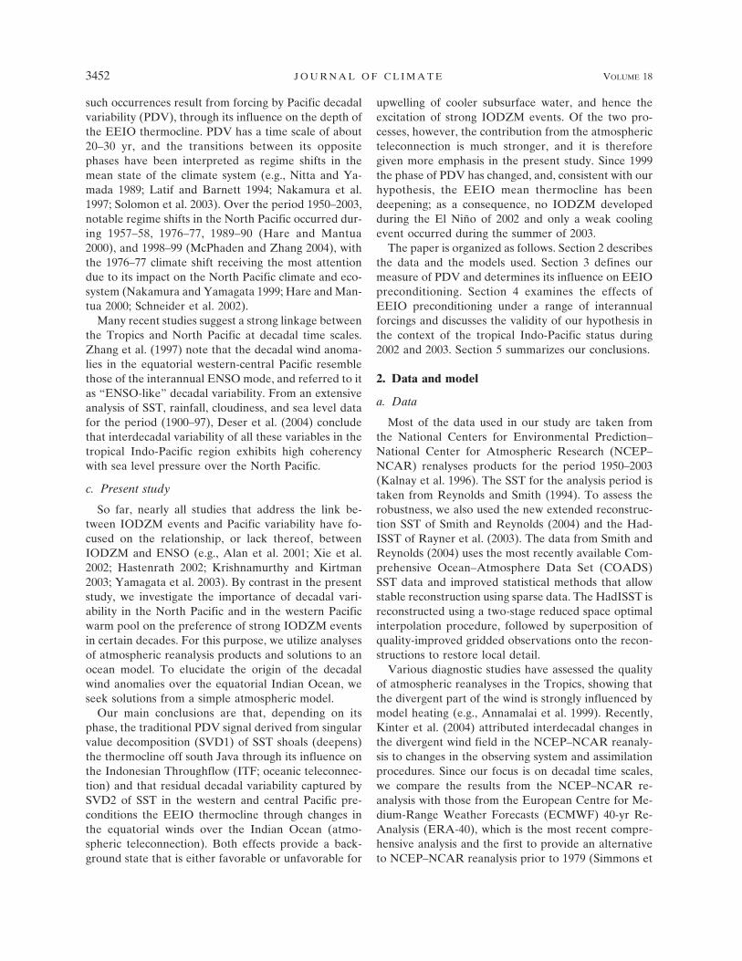
As a measure of the IODZM, Fig. 1a plots the inter-annual SST anomalies during June–November aver-aged over the region 10°S–0°, 90°–110°E, as determinedfrom Reynolds and Smith (1994; Fig. 1a), Smith andReynolds (200; Fig. 1b), and the Hadley Centre inter-polated SST (HadISST) dataset of Rayner et al. (2003;

Fig. 1c; details of the data are given in section 2). Thethree SST indices show that during the last four–fivedecades, almost all of the strong IODZM events withamplitudes close to or greater than one standard devia-tion occurred during the 1960s and 1990s, the sole ex-ception being the 1982 event. (For convenience,throughout the paper we refer to the period 1960–69 asthe 1960s, 1970–77 as the 1970s, 1980–89 as the 1980s,and 1990–97 as the 1990s). Typically, strong events areprominent in the decades of the 1960s and 1990s, andthey are weak or quiescent at other times.

b. Influence of PDV

An obvious question that emerges from Fig. 1 is whatcauses the preference of strong IODZM events in cer-tain decades? A possibility explored in this paper is that

FIG. 1. Interannual SST anomalies (in std dev) over the EEIO (10°S–0°, 90°–110°E) aver-aged during Jun–Nov from three different SST products: (a) Reynolds and Smith (1994), (b)Smith and Reynolds (2004), and (c) HadISST of Rayner et al. (2003). The dotted horizontallines correspond to 1.0 std dev.

1 SEPTEMBER 2005 A N N A M A L A I E T A L . 3451

such occurrences result from forcing by Pacific decadalvariability (PDV), through its influence on the depth ofthe EEIO thermocline. PDV has a time scale of about20–30 yr, and the transitions between its oppositephases have been interpreted as regime shifts in themean state of the climate system (e.g., Nitta and Ya-mada 1989; Latif and Barnett 1994; Nakamura et al.1997; Solomon et al. 2003). Over the period 1950–2003,notable regime shifts in the North Pacific occurred dur-ing 1957–58, 1976–77, 1989–90 (Hare and Mantua2000), and 1998–99 (McPhaden and Zhang 2004), withthe 1976–77 climate shift receiving the most attentiondue to its impact on the North Pacific climate and eco-system (Nakamura and Yamagata 1999; Hare and Man-tua 2000; Schneider et al. 2002).

Many recent studies suggest a strong linkage betweenthe Tropics and North Pacific at decadal time scales.Zhang et al. (1997) note that the decadal wind anoma-lies in the equatorial western-central Pacific resemblethose of the interannual ENSO mode, and referred to itas “ENSO-like” decadal variability. From an extensiveanalysis of SST, rainfall, cloudiness, and sea level datafor the period (1900–97), Deser et al. (2004) concludethat interdecadal variability of all these variables in thetropical Indo-Pacific region exhibits high coherencywith sea level pressure over the North Pacific.

c. Present study

So far, nearly all studies that address the link be-tween IODZM events and Pacific variability have fo-cused on the relationship, or lack thereof, betweenIODZM and ENSO (e.g., Alan et al. 2001; Xie et al.2002; Hastenrath 2002; Krishnamurthy and Kirtman2003; Yamagata et al. 2003). By contrast in the presentstudy, we investigate the importance of decadal vari-ability in the North Pacific and in the western Pacificwarm pool on the preference of strong IODZM eventsin certain decades. For this purpose, we utilize analysesof atmospheric reanalysis products and solutions to anocean model. To elucidate the origin of the decadalwind anomalies over the equatorial Indian Ocean, weseek solutions from a simple atmospheric model.

Our main conclusions are that, depending on itsphase, the traditional PDV signal derived from singularvalue decomposition (SVD1) of SST shoals (deepens)the thermocline off south Java through its influence onthe Indonesian Throughflow (ITF; oceanic teleconnec-tion) and that residual decadal variability captured bySVD2 of SST in the western and central Pacific pre-conditions the EEIO thermocline through changes inthe equatorial winds over the Indian Ocean (atmo-spheric teleconnection). Both effects provide a back-ground state that is either favorable or unfavorable for

upwelling of cooler subsurface water, and hence theexcitation of strong IODZM events. Of the two pro-cesses, however, the contribution from the atmosphericteleconnection is much stronger, and it is thereforegiven more emphasis in the present study. Since 1999the phase of PDV has changed, and, consistent with ourhypothesis, the EEIO mean thermocline has beendeepening; as a consequence, no IODZM developedduring the El Niño of 2002 and only a weak coolingevent occurred during the summer of 2003.

The paper is organized as follows. Section 2 describesthe data and the models used. Section 3 defines ourmeasure of PDV and determines its influence on EEIOpreconditioning. Section 4 examines the effects ofEEIO preconditioning under a range of interannualforcings and discusses the validity of our hypothesis inthe context of the tropical Indo-Pacific status during2002 and 2003. Section 5 summarizes our conclusions.

2. Data and model

a. Data

Most of the data used in our study are taken fromthe National Centers for Environmental Prediction–National Center for Atmospheric Research (NCEP–NCAR) renalyses products for the period 1950–2003(Kalnay et al. 1996). The SST for the analysis period istaken from Reynolds and Smith (1994). To assess therobustness, we also used the new extended reconstruc-tion SST of Smith and Reynolds (2004) and the Had-ISST of Rayner et al. (2003). The data from Smith andReynolds (2004) uses the most recently available Com-prehensive Ocean–Atmosphere Data Set (COADS)SST data and improved statistical methods that allowstable reconstruction using sparse data. The HadISST isreconstructed using a two-stage reduced space optimalinterpolation procedure, followed by superposition ofquality-improved gridded observations onto the recon-structions to restore local detail.

Various diagnostic studies have assessed the qualityof atmospheric reanalyses in the Tropics, showing thatthe divergent part of the wind is strongly influenced bymodel heating (e.g., Annamalai et al. 1999). Recently,Kinter et al. (2004) attributed interdecadal changes inthe divergent wind field in the NCEP–NCAR reanaly-sis to changes in the observing system and assimilationprocedures. Since our focus is on decadal time scales,we compare the results from the NCEP–NCAR re-analysis with those from the European Centre for Me-dium-Range Weather Forecasts (ECMWF) 40-yr Re-Analysis (ERA-40), which is the most recent compre-hensive analysis and the first to provide an alternativeto NCEP–NCAR reanalysis prior to 1979 (Simmons et


al. 2004). ERA-40 is available from September 1957 toAugust 2002 and more details can be found in Simmonset al. (2004).

Additionally, we use the thermocline depth informa-tion from the new ocean reanalysis product, the SimpleOcean Data Assimilation (SODA) Parallel Ocean Pro-gram (POP). The major change that distinguishes thisreanalysis from previous SODA efforts is that theocean model has changed, and is now at a much higherresolution. Briefly, the ocean model used is an inter-mediate resolution version of the POP code developedat the Los Alamos National Laboratories. The model’sspatial domain is global in extent, with a grid that has aresolution of 0.4° of longitude and 0.28° of latitude. Themodel has 40 vertical levels, which vary in depth from10 m at the surface to 250 m in the deep ocean. Themodel is forced with daily averaged winds from ERA-40 reanalysis spanning the period from January 1958 to2001. Surface freshwater flux for the period 1979–2001is provided by a combination of Global PrecipitationClimatology Project monthly merged product com-bined with evaporation obtained from bulk formula.Bulk formulas are also used for the surface heat flux.SST is assimilated from observations (not a relaxation).Details of the reanalysis are provided in an upcomingarticle by J. A. Carton and B. S. Giese (2005, personalcommunication).

b. Models

1) OCEAN MODEL

The model ocean is a reduced-gravity, primitive equa-tion, sigma-coordinate model coupled to an advective at-mospheric mixed-layer model (Chen et al. 1994). Themodel domain extends over the Indo-Pacific region:55°S–45°N, 30°E–70°W. The horizontal resolution is 0.3°within 10°S–10°N increasing up to 0.75° at 50°S and 45°N.The longitudinal resolution is uniform at 0.5° while thevertical resolution is of the order of 2 m below the mixedlayer increasing up to 10 at 100 m. There are 25 sigmalayers in the vertical with five layers in the top 10 m. Thebottom of the active layers typically extends to about1500 m in the Tropics. Surface heat fluxes are computedfrom the atmospheric mixed layer using model SST,with specified Earth Radiation Budget Experiment(ERBE) solar radiation, International Satellite CloudClimatology Project (ISCCP) cloudiness, and Xie andArkin (1996) precipitation; due to the lack of reliable longtime series, we specify climatological monthly-mean val-ues for these variables. Open boundaries in the north andsouth are relaxed to Levitus and Boyer (1994) climato-logical temperature and salinity profiles over a 5° spongelayer. We note that the model has already been success-

fully used in a number of applications similar to ours.For example, it simulates well the seasonal-to-interannual variability of the ITF (Murtugudde et al.1998a) and SST in the tropical Indian and PacificOceans (Murtugudde et al. 2000; Hackert et al. 2001).

A key model diagnostic is thermocline depth, h(x, y,t), which we measure by the position of the 24°C iso-therm, a typical value for the upper thermocline in theEEIO. As indicated by vertical modes of variability forpropagating waves in the region, this isotherm is morerepresentative of upper-ocean variations than midther-mocline ones (Potemra et al. 2003). Moreover, its ver-tical motions measure the upwelling of cold water intothe mixed layer more accurately than the 20°C iso-therm, which is typically used to measure thermocline-depth variations in other regions.

Table 1 lists the experiments that we report and theirrespective wind forcings. The model was initially “spunup” for 45 yr with climatological, daily wind stress fromthe NCEP–NCAR reanalysis (control or CTL run).The “interannual” run (INT) was initialized by the spunup run and forced with interannually varying, dailymean, NCEP reanalysis winds. Thus, the interannualvariability in INT is driven by interannual wind stresses,which in turn affect the latent and sensible heat fluxesthrough their influence on wind speed, and these forc-ings generate realistic SST anomalies in both oceans.The other test runs are extensions forced by climato-logical winds plus specified anomalies described below.Since the model is spun up for 40 yr with climatologicalwinds it has no spinup or cold-start problems to im-posed anomalies.

2) SIMPLE LINEAR ATMOSPHERIC MODEL

The model used here, which we refer to as the linearbaroclinic model (LBM), is described in detail in Wa-

TABLE 1. A list of the ocean model experiments discussed inthe text.

Expts ForcingTime(yr)

INT NCEP winds 52CTL Climate NCEP winds 45EAST CTL � Indian Ocean easterlies 5WEST CTL � Indian Ocean westerlies 5EAST97 EAST, then 1997 winds 1WEST97 WEST, then 1997 winds 1CTL97 CTL, then 1997 winds 1EAST61 EAST, then 1961 winds 1WEST61 WEST, then 1961 winds 1EAST96 EAST, then 1996 winds 1WEST96 WEST, then 1996 winds 1EAST57 EAST, then 57 winds 1WEST57 WEST, then 57 winds 1


tanabe and Kimoto (2000) and Watanabe and Jin(2003). It is a global, time-dependent, primitive equa-tion model, linearized about the observed climatologyderived from NCEP–NCAR reanalysis. Its horizontalresolution has triangular truncation 42 and there are 20vertical levels in sigma coordinates. The model employsdiffusion, Rayleigh friction, and Newtonian dampingwith a time scale of (1 day)�1 for � � 0.9 and � � 0.03,while (30 day)�1 is used elsewhere. The surface heatfluxes due to imposed SST anomalies and cumulus con-vection (Betts and Miller 1986) are parameterized, anda linearized moisture equation for the perturbation spe-cific humidity is incorporated into the model. More de-tails can be found in Watanabe and Jin (2003). In theLBM, the steady-state response may depend on themean state about which linearization is sought (e.g.,Gill 1980). Due to the decadal time scale nature of thesignals, linearization about the annual-mean climatol-ogy is considered. The LBM is integrated for 30 days,and, with the dissipation terms adopted, the tropicalresponse approaches a steady state after day 10. Theresponse at day 20 is analyzed.

c. Data processing

In the data and ocean model analyses reported here,monthly-mean climatologies are first calculated for thestudy period and anomalies are departures from them.Unless specified otherwise, decadal variability (periods�8 yr) is separated from interannual variability (16months to 8 yr) through harmonic analysis, in order toinvestigate possible links between the two time scales.It should be stressed here that since we have filteredout interannual variability, the decadal component isnot contaminated by interannual IODZM events andtherefore accounts for the slow variation in the climatesystem. Similar interpretations of this “linear” indepen-dency between interannual and decadal ENSO-likevariability have been done in past studies (e.g., Pierceet al. 2000).

3. Preconditioning of the EEIO thermocline

In this section, we report several analyses that relatePDV to decadal variability in the Indo-Pacific Tropics.First, we perform a SVD analysis on decadal SST, sur-face winds, and h from solution INT (section 3a) whichidentifies the importance of decadal signals from thePacific in preconditioning the EEIO thermocline. Next,we construct a measure of EEIO preconditioning, I,based on h (section 3b). Then, we force the LBM withSST patterns obtained from the SVD analysis to con-firm the role of Pacific SST in forcing equatorial wind

anomalies over the Indian Ocean (section 3c). Finally,we force the ocean model with idealized wind stressanomaly patterns over the equatorial Indian Ocean tocreate the EEIO preconditioning (section 3d).

a. SVD analysis

SVD is a fundamental matrix operation, a general-ization of the diagonalization method that is performedin principal component (PC) analysis to matrices thatare not square or symmetric. A unique benefit is thatSVD of a cross-covariance matrix identifies, say fromtwo data fields, pairs of spatial patterns that explain asmuch as possible of the mean-squared temporal covari-ance between the two fields. More details of themethod are in Bretherton et al. (1992). In the presentstudy, we have used three variables and the cross-covariance terms among them are given as input tothe SVD analysis. To verify the results shown below,we carried out separate SVD analysis where cross-covariance terms between pairs of variables (viz., SSTand surface winds, SST and h, and surface winds and h)are given as input, and the results (not shown) remainconsistent with the ones discussed below.

1) SVD RESULTS FROM PACIFIC SSTA

Figures 2–4 show the spatial structures and PCs ofthe first two SVDs determined from low-pass-filtered(periods �8 yr) SST data over the region (20°S–60°N,120°E–80°W), surface winds over the Indo-PacificTropics (30°S–30°N, 40°E–80°W), and h over the tropi-cal Indian Ocean (20°S–20°N, 55°–120°E). The eigen-values of the first two SVD are well separated fromhigher-order patterns.

The SST spatial pattern of SVD1 (Fig. 2a) closelyresembles the PDV in the North Pacific and ENSO-likedecadal variability in the tropical Pacific that has beenidentified in many previous studies (e.g., Zhang et al.1997; Nakamura et al. 1997; Pierce et al. 2000). Theassociated surface wind variability (Fig. 2b) in the Pa-cific depicts weakening of the easterly trade winds witha fair degree of equatorial symmetry, implying ElNiño–like conditions. Other notable features in Fig. 2binclude low-level divergence over the equatorial westPacific and enhanced easterly (westerly) wind anoma-lies to the south of Sumatran coast (equatorial westernIndian Ocean). The covarying signal in h (Fig. 2c) in-dicates a shallowing of the thermocline off south Java(8°–14°S, 105°–120°E), and deepening in the entireequatorial Indian Ocean, with a maximum in the west.The associated time dependence, PC1 (Fig. 4a), under-goes a prominent switch from negative-to-positive val-ues during the 1976–77 climate shift. Apart from this


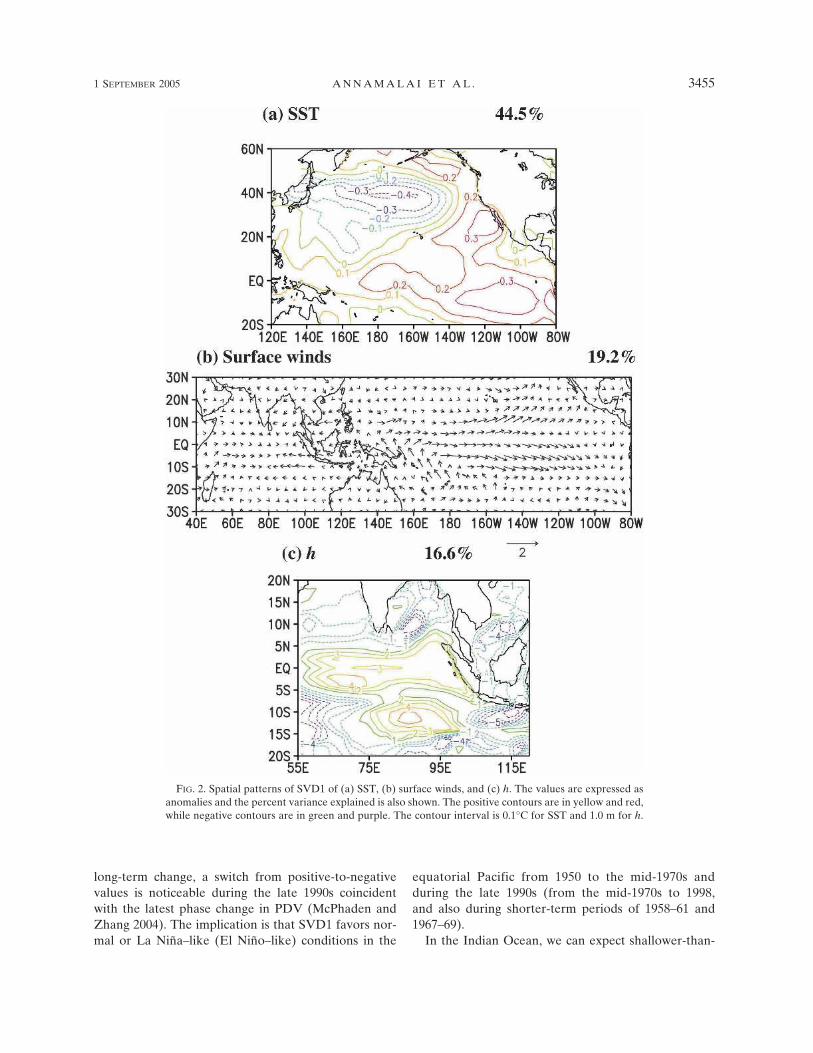
long-term change, a switch from positive-to-negativevalues is noticeable during the late 1990s coincidentwith the latest phase change in PDV (McPhaden andZhang 2004). The implication is that SVD1 favors nor-mal or La Niña–like (El Niño–like) conditions in the

equatorial Pacific from 1950 to the mid-1970s andduring the late 1990s (from the mid-1970s to 1998,and also during shorter-term periods of 1958–61 and1967–69).

In the Indian Ocean, we can expect shallower-than-

FIG. 2. Spatial patterns of SVD1 of (a) SST, (b) surface winds, and (c) h. The values are expressed asanomalies and the percent variance explained is also shown. The positive contours are in yellow and red,while negative contours are in green and purple. The contour interval is 0.1°C for SST and 1.0 m for h.


Fig 2 live 4/C

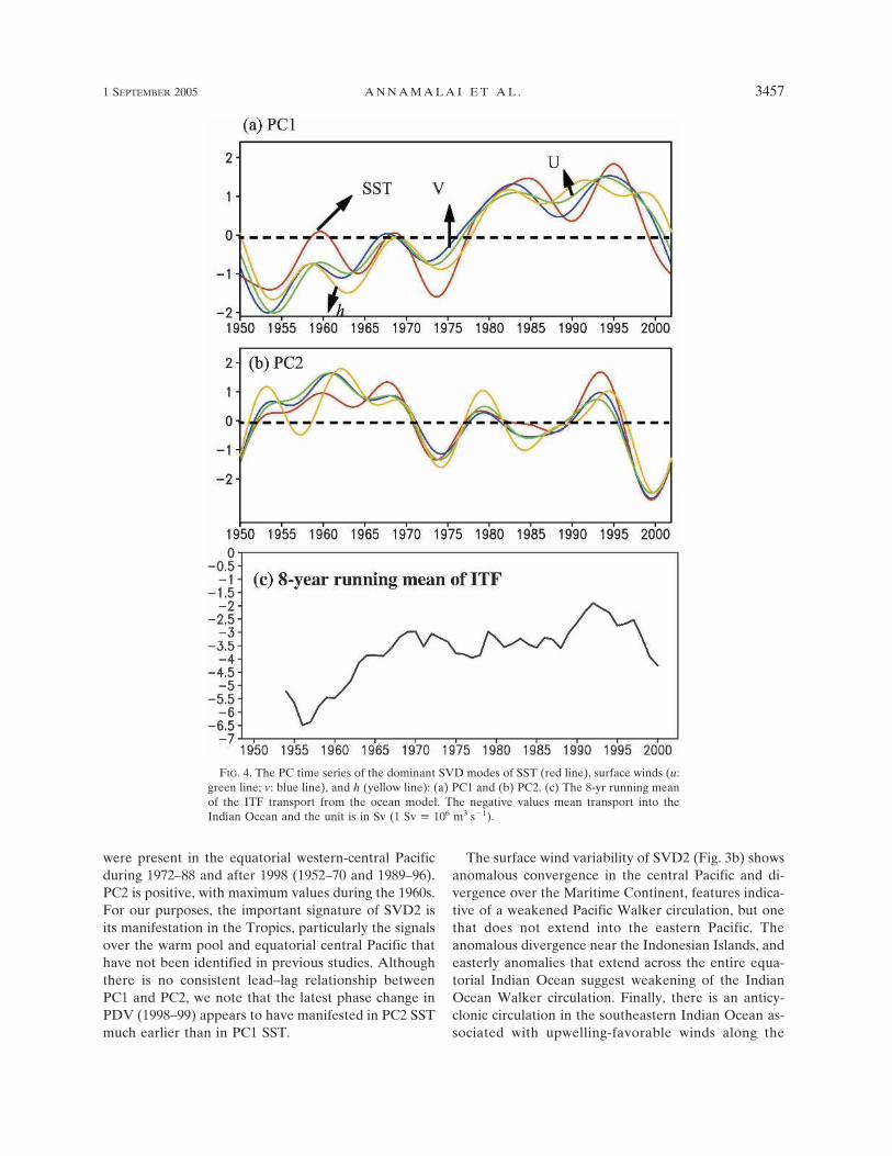
normal h in the south Java region during 1976–97, anddeeper than normal h during most of 1950–76 and after1998. The thermocline variations off south Java are par-ticularly related to the variations in the ITF transportthrough the Lombak strait (e.g., Meyers 1996). Thedecadal variability of ITF transport in the model (Fig.4c) shows a general decrease from the mid-1950s toearly 1970s with a large reduction in the late 1980s and

early 1990s. This relationship suggests that the equato-rial winds along the entire Pacific during El Niño–likeconditions reduces the ITF and results in the h shoalingoff south Java, consistent with other studies (e.g., Su-santo et al. 2001; Potemra et al. 2003).

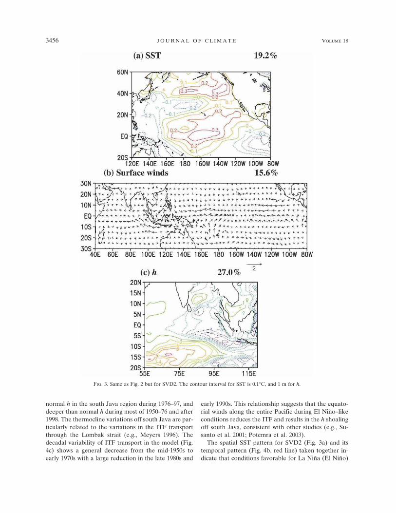
The spatial SST pattern for SVD2 (Fig. 3a) and itstemporal pattern (Fig. 4b, red line) taken together in-dicate that conditions favorable for La Niña (El Niño)

FIG. 3. Same as Fig. 2 but for SVD2. The contour interval for SST is 0.1°C, and 1 m for h.


Fig 3 live 4/C

were present in the equatorial western-central Pacificduring 1972–88 and after 1998 (1952–70 and 1989–96).PC2 is positive, with maximum values during the 1960s.For our purposes, the important signature of SVD2 isits manifestation in the Tropics, particularly the signalsover the warm pool and equatorial central Pacific thathave not been identified in previous studies. Althoughthere is no consistent lead–lag relationship betweenPC1 and PC2, we note that the latest phase change inPDV (1998–99) appears to have manifested in PC2 SSTmuch earlier than in PC1 SST.

The surface wind variability of SVD2 (Fig. 3b) showsanomalous convergence in the central Pacific and di-vergence over the Maritime Continent, features indica-tive of a weakened Pacific Walker circulation, but onethat does not extend into the eastern Pacific. Theanomalous divergence near the Indonesian Islands, andeasterly anomalies that extend across the entire equa-torial Indian Ocean suggest weakening of the IndianOcean Walker circulation. Finally, there is an anticy-clonic circulation in the southeastern Indian Ocean as-sociated with upwelling-favorable winds along the

FIG. 4. The PC time series of the dominant SVD modes of SST (red line), surface winds (u:green line; v: blue line), and h (yellow line): (a) PC1 and (b) PC2. (c) The 8-yr running meanof the ITF transport from the ocean model. The negative values mean transport into theIndian Ocean and the unit is in Sv (1 Sv � 106 m3 s�1).


Fig 4 live 4/C

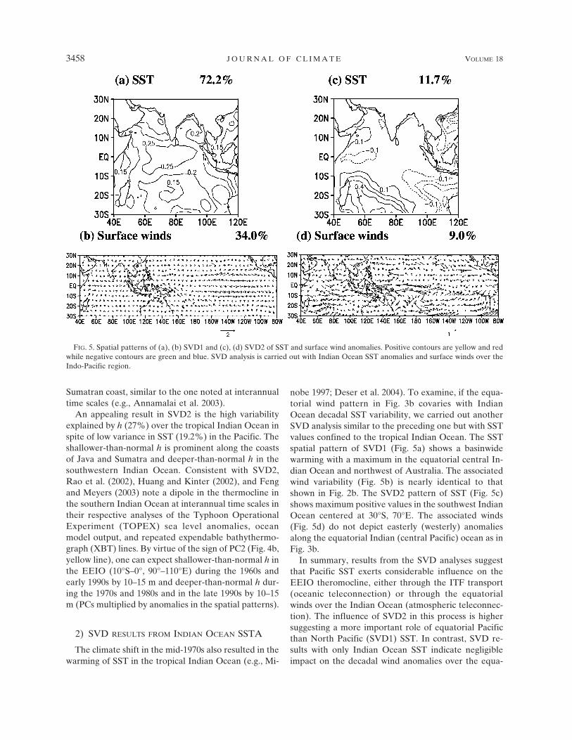
Sumatran coast, similar to the one noted at interannualtime scales (e.g., Annamalai et al. 2003).

An appealing result in SVD2 is the high variabilityexplained by h (27%) over the tropical Indian Ocean inspite of low variance in SST (19.2%) in the Pacific. Theshallower-than-normal h is prominent along the coastsof Java and Sumatra and deeper-than-normal h in thesouthwestern Indian Ocean. Consistent with SVD2,Rao et al. (2002), Huang and Kinter (2002), and Fengand Meyers (2003) note a dipole in the thermocline inthe southern Indian Ocean at interannual time scales intheir respective analyses of the Typhoon OperationalExperiment (TOPEX) sea level anomalies, oceanmodel output, and repeated expendable bathythermo-graph (XBT) lines. By virtue of the sign of PC2 (Fig. 4b,yellow line), one can expect shallower-than-normal h inthe EEIO (10°S–0°, 90°–110°E) during the 1960s andearly 1990s by 10–15 m and deeper-than-normal h dur-ing the 1970s and 1980s and in the late 1990s by 10–15m (PCs multiplied by anomalies in the spatial patterns).

2) SVD RESULTS FROM INDIAN OCEAN SSTA

The climate shift in the mid-1970s also resulted in thewarming of SST in the tropical Indian Ocean (e.g., Mi-

nobe 1997; Deser et al. 2004). To examine, if the equa-torial wind pattern in Fig. 3b covaries with IndianOcean decadal SST variability, we carried out anotherSVD analysis similar to the preceding one but with SSTvalues confined to the tropical Indian Ocean. The SSTspatial pattern of SVD1 (Fig. 5a) shows a basinwidewarming with a maximum in the equatorial central In-dian Ocean and northwest of Australia. The associatedwind variability (Fig. 5b) is nearly identical to thatshown in Fig. 2b. The SVD2 pattern of SST (Fig. 5c)shows maximum positive values in the southwest IndianOcean centered at 30°S, 70°E. The associated winds(Fig. 5d) do not depict easterly (westerly) anomaliesalong the equatorial Indian (central Pacific) ocean as inFig. 3b.

In summary, results from the SVD analyses suggestthat Pacific SST exerts considerable influence on theEEIO theromocline, either through the ITF transport(oceanic teleconnection) or through the equatorialwinds over the Indian Ocean (atmospheric teleconnec-tion). The influence of SVD2 in this process is highersuggesting a more important role of equatorial Pacificthan North Pacific (SVD1) SST. In contrast, SVD re-sults with only Indian Ocean SST indicate negligibleimpact on the decadal wind anomalies over the equa-

FIG. 5. Spatial patterns of (a), (b) SVD1 and (c), (d) SVD2 of SST and surface wind anomalies. Positive contours are yellow and redwhile negative contours are green and blue. SVD analysis is carried out with Indian Ocean SST anomalies and surface winds over theIndo-Pacific region.


torial Indian Ocean, and we therefore infer that PDV isthe primary agent for preconditioning the EEIO ther-mocline. We repeated SVD calculations with the twonew SST products (section 2) and noted no changes tothe results.

b. Index of EEIO preconditioning

A key assumption in our discussion is that IODZMevents are favored only when h is shallow enough in theEEIO for SST to cool below 27.5°C, the threshold re-quired for deep convection in the Tropics (e.g., Grahamand Barnett 1987). Accordingly, we constructed a mea-sure for EEIO preconditioning, I, based on h. Let �h1and �h2 be the average value of anomalous h in theEEIO domain determined from the SVD1 and SVD2patterns (Figs. 2c and 3c). Then,

I � PC1 � �h1 � PC2 � �h2. 1

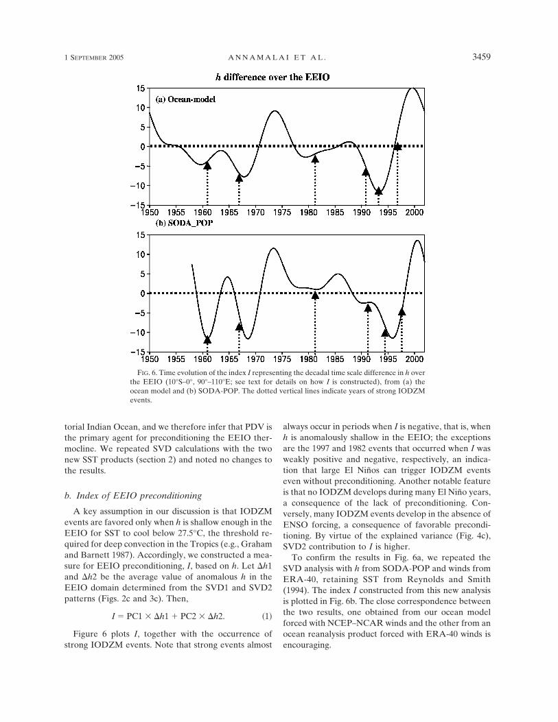
Figure 6 plots I, together with the occurrence ofstrong IODZM events. Note that strong events almost

always occur in periods when I is negative, that is, whenh is anomalously shallow in the EEIO; the exceptionsare the 1997 and 1982 events that occurred when I wasweakly positive and negative, respectively, an indica-tion that large El Niños can trigger IODZM eventseven without preconditioning. Another notable featureis that no IODZM develops during many El Niño years,a consequence of the lack of preconditioning. Con-versely, many IODZM events develop in the absence ofENSO forcing, a consequence of favorable precondi-tioning. By virtue of the explained variance (Fig. 4c),SVD2 contribution to I is higher.

To confirm the results in Fig. 6a, we repeated theSVD analysis with h from SODA-POP and winds fromERA-40, retaining SST from Reynolds and Smith(1994). The index I constructed from this new analysisis plotted in Fig. 6b. The close correspondence betweenthe two results, one obtained from our ocean modelforced with NCEP–NCAR winds and the other from anocean reanalysis product forced with ERA-40 winds isencouraging.

FIG. 6. Time evolution of the index I representing the decadal time scale difference in h overthe EEIO (10°S–0°, 90°–110°E; see text for details on how I is constructed), from (a) theocean model and (b) SODA-POP. The dotted vertical lines indicate years of strong IODZMevents.


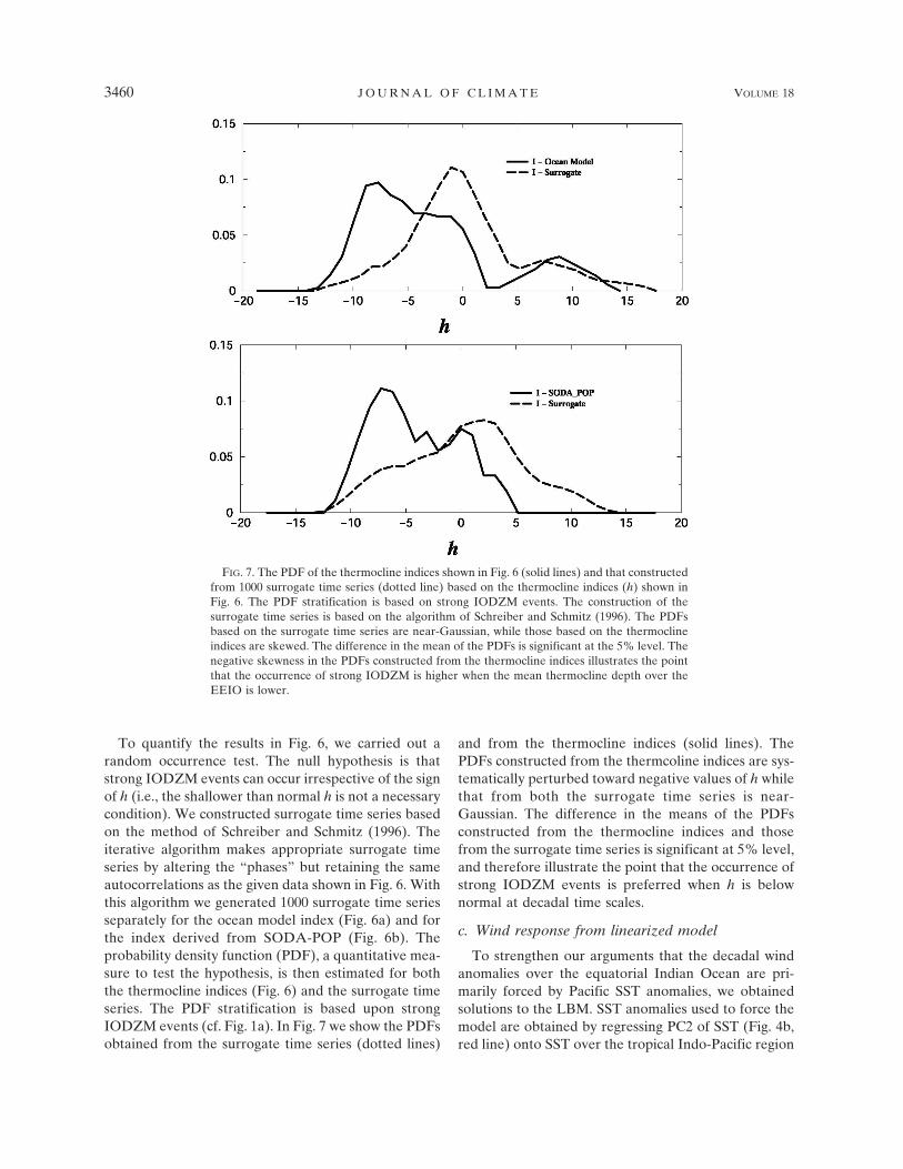
To quantify the results in Fig. 6, we carried out arandom occurrence test. The null hypothesis is thatstrong IODZM events can occur irrespective of the signof h (i.e., the shallower than normal h is not a necessarycondition). We constructed surrogate time series basedon the method of Schreiber and Schmitz (1996). Theiterative algorithm makes appropriate surrogate timeseries by altering the “phases” but retaining the sameautocorrelations as the given data shown in Fig. 6. Withthis algorithm we generated 1000 surrogate time seriesseparately for the ocean model index (Fig. 6a) and forthe index derived from SODA-POP (Fig. 6b). Theprobability density function (PDF), a quantitative mea-sure to test the hypothesis, is then estimated for boththe thermocline indices (Fig. 6) and the surrogate timeseries. The PDF stratification is based upon strongIODZM events (cf. Fig. 1a). In Fig. 7 we show the PDFsobtained from the surrogate time series (dotted lines)

and from the thermocline indices (solid lines). ThePDFs constructed from the thermcoline indices are sys-tematically perturbed toward negative values of h whilethat from both the surrogate time series is near-Gaussian. The difference in the means of the PDFsconstructed from the thermocline indices and thosefrom the surrogate time series is significant at 5% level,and therefore illustrate the point that the occurrence ofstrong IODZM events is preferred when h is belownormal at decadal time scales.

c. Wind response from linearized model

To strengthen our arguments that the decadal windanomalies over the equatorial Indian Ocean are pri-marily forced by Pacific SST anomalies, we obtainedsolutions to the LBM. SST anomalies used to force themodel are obtained by regressing PC2 of SST (Fig. 4b,red line) onto SST over the tropical Indo-Pacific region

FIG. 7. The PDF of the thermocline indices shown in Fig. 6 (solid lines) and that constructedfrom 1000 surrogate time series (dotted line) based on the thermocline indices (h) shown inFig. 6. The PDF stratification is based on strong IODZM events. The construction of thesurrogate time series is based on the algorithm of Schreiber and Schmitz (1996). The PDFsbased on the surrogate time series are near-Gaussian, while those based on the thermoclineindices are skewed. The difference in the mean of the PDFs is significant at the 5% level. Thenegative skewness in the PDFs constructed from the thermocline indices illustrates the pointthat the occurrence of strong IODZM is higher when the mean thermocline depth over theEEIO is lower.


(not shown). Apart from retaining the spatial patternshown in Fig. 3a, cold SST anomalies over the south-eastern tropical Indian Ocean (as noted in Fig. 5c) arealso apparent in the regression analysis. To understandthe individual and collective roles of SST anomalies invarious regions on the wind patterns, we carried outfour experiments with SST patterns over (i) southeast-ern tropical Indian Ocean, (ii) tropical western Pacific,(iii) equatorial central Pacific, and (iv) the near-equatorial eastern Pacific. Of the four experiments, theresponse to both southeastern tropical Indian Ocean

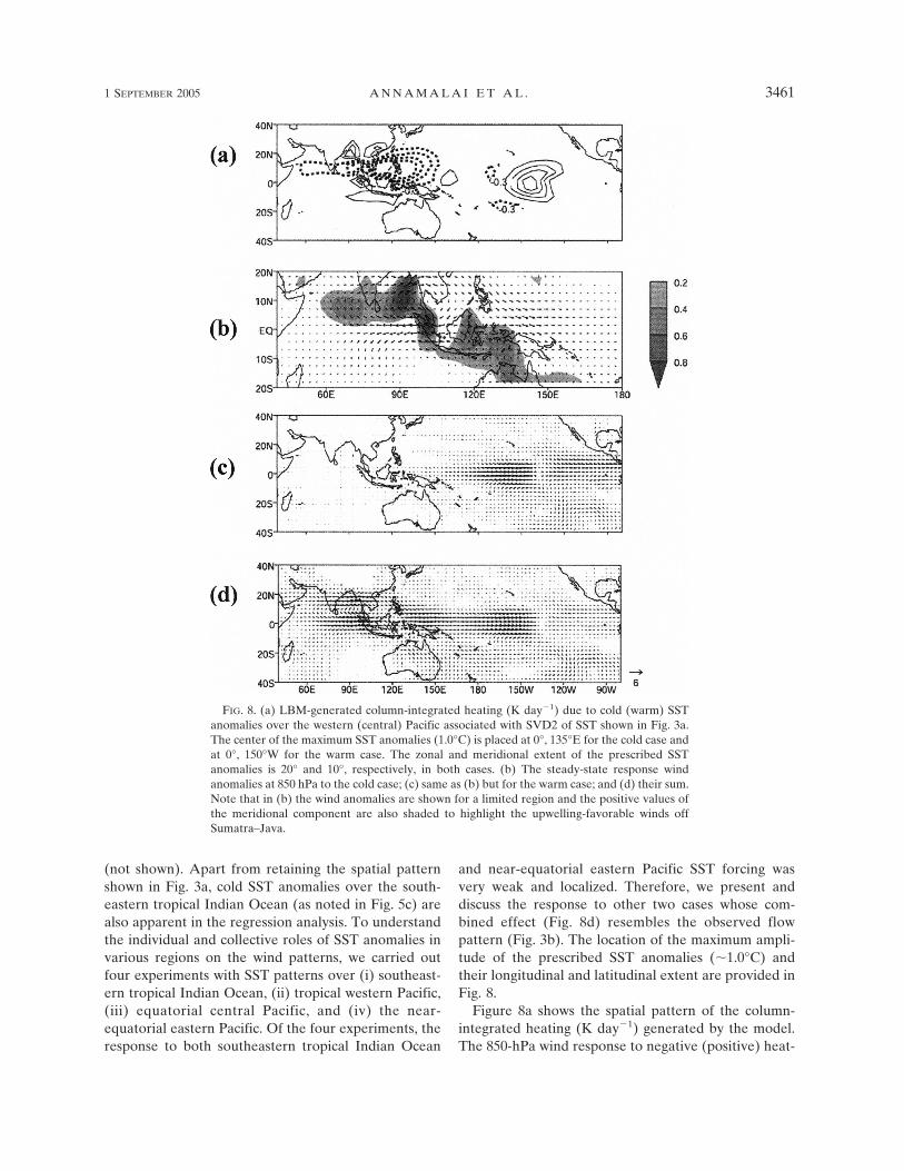
and near-equatorial eastern Pacific SST forcing wasvery weak and localized. Therefore, we present anddiscuss the response to other two cases whose com-bined effect (Fig. 8d) resembles the observed flowpattern (Fig. 3b). The location of the maximum ampli-tude of the prescribed SST anomalies (�1.0°C) andtheir longitudinal and latitudinal extent are provided inFig. 8.

Figure 8a shows the spatial pattern of the column-integrated heating (K day�1) generated by the model.The 850-hPa wind response to negative (positive) heat-

FIG. 8. (a) LBM-generated column-integrated heating (K day�1) due to cold (warm) SSTanomalies over the western (central) Pacific associated with SVD2 of SST shown in Fig. 3a.The center of the maximum SST anomalies (1.0°C) is placed at 0°, 135°E for the cold case andat 0°, 150°W for the warm case. The zonal and meridional extent of the prescribed SSTanomalies is 20° and 10°, respectively, in both cases. (b) The steady-state response windanomalies at 850 hPa to the cold case; (c) same as (b) but for the warm case; and (d) their sum.Note that in (b) the wind anomalies are shown for a limited region and the positive values ofthe meridional component are also shaded to highlight the upwelling-favorable winds offSumatra–Java.


ing over the western (equatorial central) Pacific isshown in Fig. 8b (Fig. 8c). The Kelvin wave response towestern Pacific heating generates westerly anomalies inthe equatorial central Pacific that are symmetric aboutthe equator. An anticyclonic circulation develops westof the heating anomalies as a Rossby wave responsecausing easterly anomalies along the equatorial IndianOcean. The shading in Fig. 8b highlights the upwelling-favorable winds off Sumatra (only positive values of themeridional component of the wind are shaded) and theLBM solutions qualitatively agree with Fig. 3b. Theresponse to central Pacific positive SST anomalies isfelt over the equatorial Pacific with a weak signatureover the equatorial Indian Ocean.

In a recent ongoing work, it is found that the areacovered by the western Pacific warm pool waxes andwanes at decadal time scales (V. Mehta 2002, personalcommunication). Consistent with that variability, theSVD2 SST pattern (Fig. 3a) captures a considerablesignal over the western Pacific warm pool. The decadalpersistence of SST anomalies over the warm pool, de-spite being small in magnitude (�0.3°–0.5°C in certaindecades like the 1960s and 1990s), may allow them tohave an appreciable influence on local convection andsubsequently on the low-level winds, as shown by theLBM experiments.

d. Influence of decadal wind anomalies in theEEIO

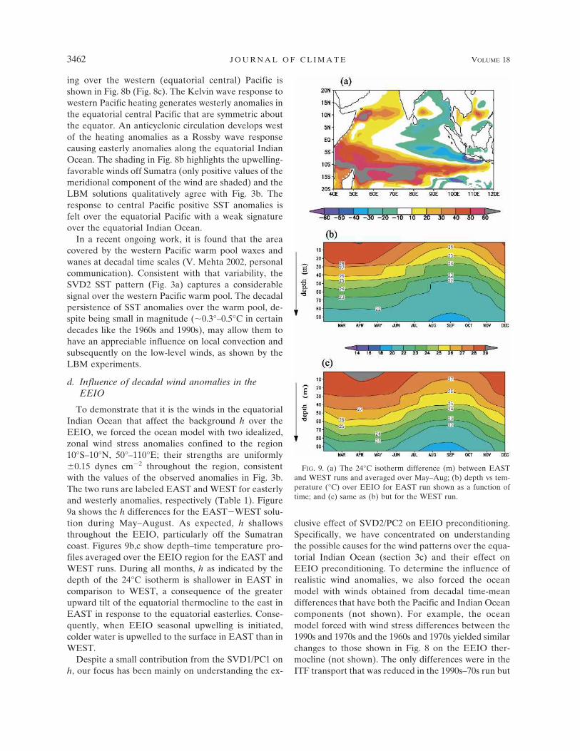
To demonstrate that it is the winds in the equatorialIndian Ocean that affect the background h over theEEIO, we forced the ocean model with two idealized,zonal wind stress anomalies confined to the region10°S–10°N, 50°–110°E; their strengths are uniformly�0.15 dynes cm�2 throughout the region, consistentwith the values of the observed anomalies in Fig. 3b.The two runs are labeled EAST and WEST for easterlyand westerly anomalies, respectively (Table 1). Figure9a shows the h differences for the EAST�WEST solu-tion during May–August. As expected, h shallowsthroughout the EEIO, particularly off the Sumatrancoast. Figures 9b,c show depth–time temperature pro-files averaged over the EEIO region for the EAST andWEST runs. During all months, h as indicated by thedepth of the 24°C isotherm is shallower in EAST incomparison to WEST, a consequence of the greaterupward tilt of the equatorial thermocline to the east inEAST in response to the equatorial easterlies. Conse-quently, when EEIO seasonal upwelling is initiated,colder water is upwelled to the surface in EAST than inWEST.

Despite a small contribution from the SVD1/PC1 onh, our focus has been mainly on understanding the ex-

clusive effect of SVD2/PC2 on EEIO preconditioning.Specifically, we have concentrated on understandingthe possible causes for the wind patterns over the equa-torial Indian Ocean (section 3c) and their effect onEEIO preconditioning. To determine the influence ofrealistic wind anomalies, we also forced the oceanmodel with winds obtained from decadal time-meandifferences that have both the Pacific and Indian Oceancomponents (not shown). For example, the oceanmodel forced with wind stress differences between the1990s and 1970s and the 1960s and 1970s yielded similarchanges to those shown in Fig. 8 on the EEIO ther-mocline (not shown). The only differences were in theITF transport that was reduced in the 1990s–70s run but

FIG. 9. (a) The 24°C isotherm difference (m) between EASTand WEST runs and averaged over May–Aug; (b) depth vs tem-perature (°C) over EEIO for EAST run shown as a function oftime; and (c) same as (b) but for the WEST run.


Fig 9 live 4/C

increased in the 1960s–70s run, and in changes to thethermocline off south Java.

4. Effect of preconditioning on IODZM events

In this section, we discuss how IODZM events areinfluenced by EEIO preconditioning and by windanomalies during their onset stage in May–June (sec-tion 4a). Then, the results of the present study are in-terpreted regarding the observed status of IndianOcean SST anomalies during the years of 2002–03 (sec-tion 4b).

a. Case studies

We carried out a suite of sensitivity experiments toinvestigate the role of wind anomalies during theIODZM event onset stage (May–June). All the experi-

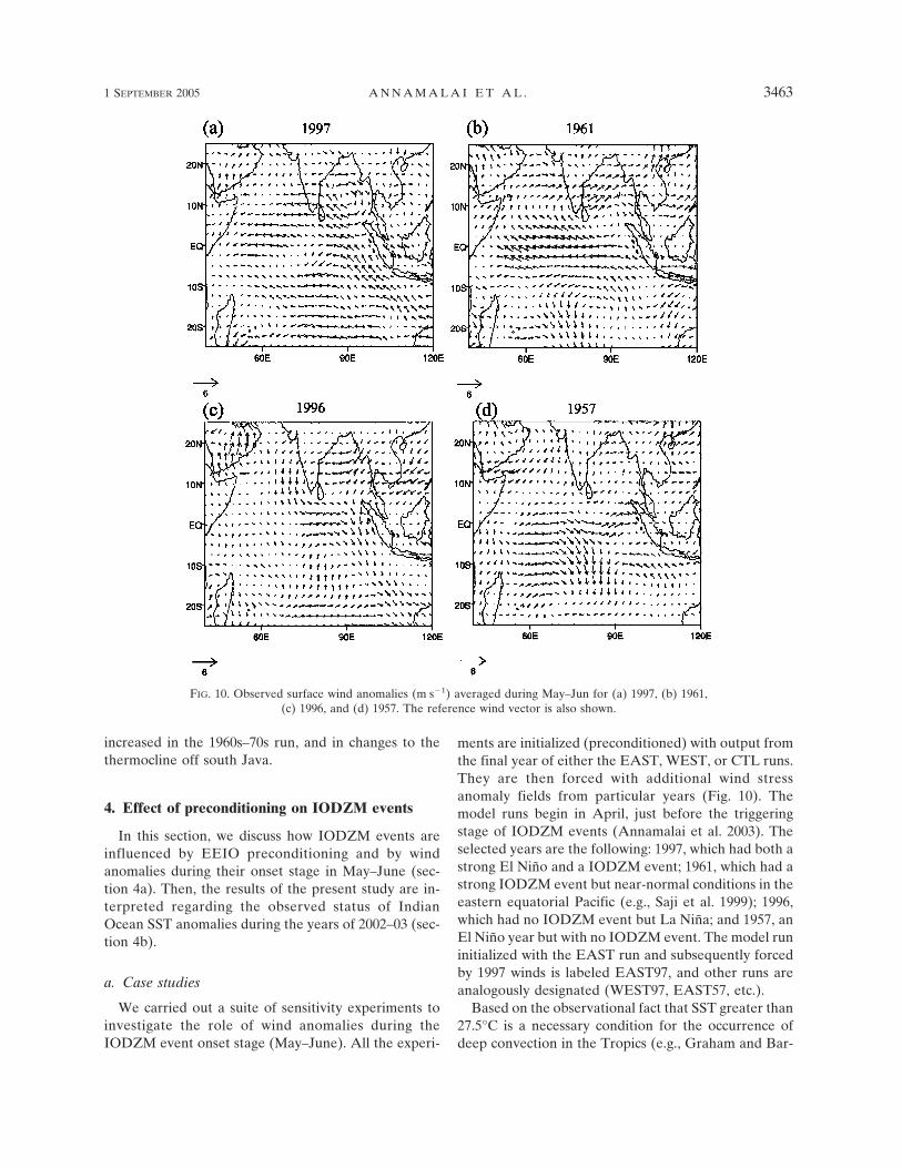
ments are initialized (preconditioned) with output fromthe final year of either the EAST, WEST, or CTL runs.They are then forced with additional wind stressanomaly fields from particular years (Fig. 10). Themodel runs begin in April, just before the triggeringstage of IODZM events (Annamalai et al. 2003). Theselected years are the following: 1997, which had both astrong El Niño and a IODZM event; 1961, which had astrong IODZM event but near-normal conditions in theeastern equatorial Pacific (e.g., Saji et al. 1999); 1996,which had no IODZM event but La Niña; and 1957, anEl Niño year but with no IODZM event. The model runinitialized with the EAST run and subsequently forcedby 1997 winds is labeled EAST97, and other runs areanalogously designated (WEST97, EAST57, etc.).

Based on the observational fact that SST greater than27.5°C is a necessary condition for the occurrence ofdeep convection in the Tropics (e.g., Graham and Bar-

FIG. 10. Observed surface wind anomalies (m s�1) averaged during May–Jun for (a) 1997, (b) 1961,(c) 1996, and (d) 1957. The reference wind vector is also shown.


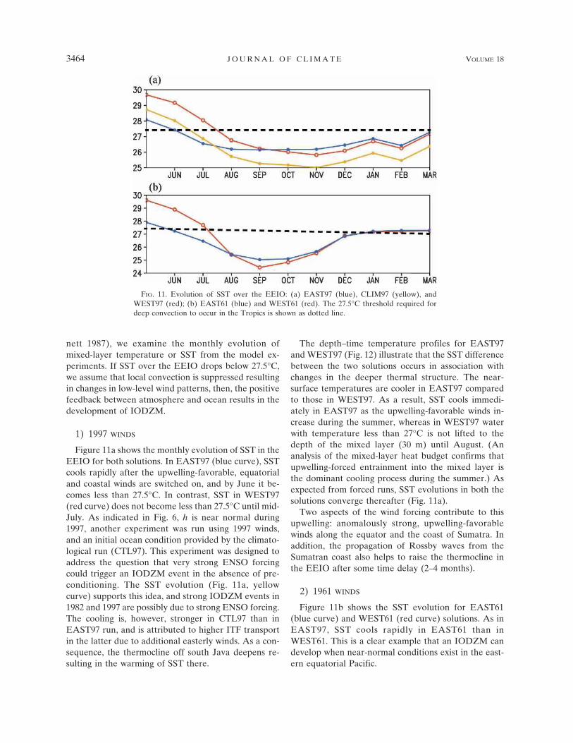
nett 1987), we examine the monthly evolution ofmixed-layer temperature or SST from the model ex-periments. If SST over the EEIO drops below 27.5°C,we assume that local convection is suppressed resultingin changes in low-level wind patterns, then, the positivefeedback between atmosphere and ocean results in thedevelopment of IODZM.

1) 1997 WINDS

Figure 11a shows the monthly evolution of SST in theEEIO for both solutions. In EAST97 (blue curve), SSTcools rapidly after the upwelling-favorable, equatorialand coastal winds are switched on, and by June it be-comes less than 27.5°C. In contrast, SST in WEST97(red curve) does not become less than 27.5°C until mid-July. As indicated in Fig. 6, h is near normal during1997, another experiment was run using 1997 winds,and an initial ocean condition provided by the climato-logical run (CTL97). This experiment was designed toaddress the question that very strong ENSO forcingcould trigger an IODZM event in the absence of pre-conditioning. The SST evolution (Fig. 11a, yellowcurve) supports this idea, and strong IODZM events in1982 and 1997 are possibly due to strong ENSO forcing.The cooling is, however, stronger in CTL97 than inEAST97 run, and is attributed to higher ITF transportin the latter due to additional easterly winds. As a con-sequence, the thermocline off south Java deepens re-sulting in the warming of SST there.

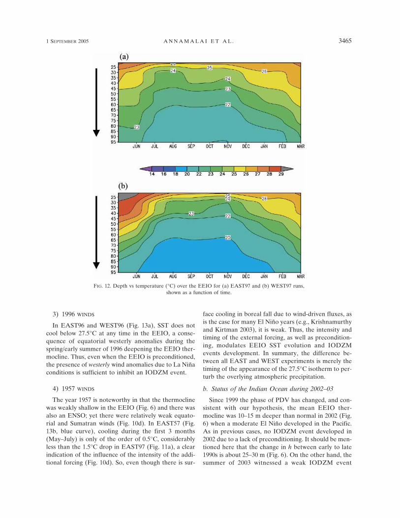
The depth–time temperature profiles for EAST97and WEST97 (Fig. 12) illustrate that the SST differencebetween the two solutions occurs in association withchanges in the deeper thermal structure. The near-surface temperatures are cooler in EAST97 comparedto those in WEST97. As a result, SST cools immedi-ately in EAST97 as the upwelling-favorable winds in-crease during the summer, whereas in WEST97 waterwith temperature less than 27°C is not lifted to thedepth of the mixed layer (30 m) until August. (Ananalysis of the mixed-layer heat budget confirms thatupwelling-forced entrainment into the mixed layer isthe dominant cooling process during the summer.) Asexpected from forced runs, SST evolutions in both thesolutions converge thereafter (Fig. 11a).

Two aspects of the wind forcing contribute to thisupwelling: anomalously strong, upwelling-favorablewinds along the equator and the coast of Sumatra. Inaddition, the propagation of Rossby waves from theSumatran coast also helps to raise the thermocline inthe EEIO after some time delay (2–4 months).

2) 1961 WINDS

Figure 11b shows the SST evolution for EAST61(blue curve) and WEST61 (red curve) solutions. As inEAST97, SST cools rapidly in EAST61 than inWEST61. This is a clear example that an IODZM candevelop when near-normal conditions exist in the east-ern equatorial Pacific.

FIG. 11. Evolution of SST over the EEIO: (a) EAST97 (blue), CLIM97 (yellow), andWEST97 (red); (b) EAST61 (blue) and WEST61 (red). The 27.5°C threshold required fordeep convection to occur in the Tropics is shown as dotted line.


Fig 11 live 4/C

3) 1996 WINDS

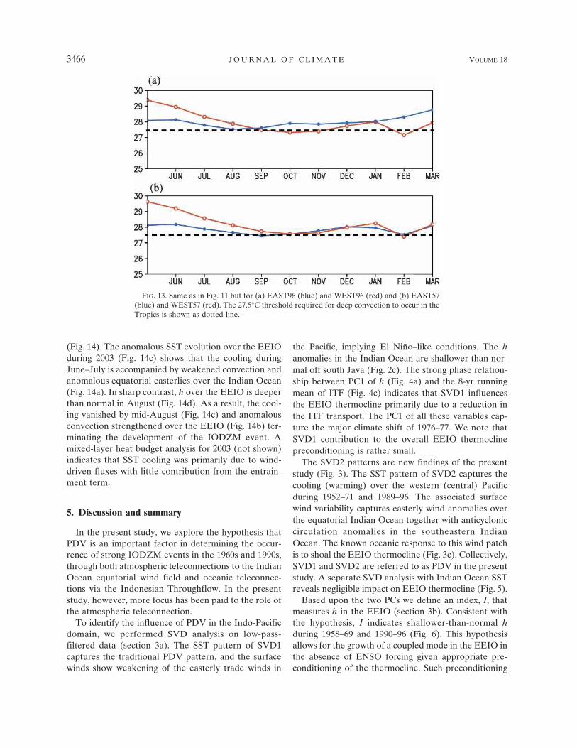
In EAST96 and WEST96 (Fig. 13a), SST does notcool below 27.5°C at any time in the EEIO, a conse-quence of equatorial westerly anomalies during thespring/early summer of 1996 deepening the EEIO ther-mocline. Thus, even when the EEIO is preconditioned,the presence of westerly wind anomalies due to La Niñaconditions is sufficient to inhibit an IODZM event.

4) 1957 WINDS

The year 1957 is noteworthy in that the thermoclinewas weakly shallow in the EEIO (Fig. 6) and there wasalso an ENSO; yet there were relatively weak equato-rial and Sumatran winds (Fig. 10d). In EAST57 (Fig.13b, blue curve), cooling during the first 3 months(May–July) is only of the order of 0.5°C, considerablyless than the 1.5°C drop in EAST97 (Fig. 11a), a clearindication of the influence of the intensity of the addi-tional forcing (Fig. 10d). So, even though there is sur-

face cooling in boreal fall due to wind-driven fluxes, asis the case for many El Niño years (e.g., Krishnamurthyand Kirtman 2003), it is weak. Thus, the intensity andtiming of the external forcing, as well as precondition-ing, modulates EEIO SST evolution and IODZMevents development. In summary, the difference be-tween all EAST and WEST experiments is merely thetiming of the appearance of the 27.5°C isotherm to per-turb the overlying atmospheric precipitation.

b. Status of the Indian Ocean during 2002–03

Since 1999 the phase of PDV has changed, and con-sistent with our hypothesis, the mean EEIO ther-mocline was 10–15 m deeper than normal in 2002 (Fig.6) when a moderate El Niño developed in the Pacific.As in previous cases, no IODZM event developed in2002 due to a lack of preconditioning. It should be men-tioned here that the change in h between early to late1990s is about 25–30 m (Fig. 6). On the other hand, thesummer of 2003 witnessed a weak IODZM event

FIG. 12. Depth vs temperature (°C) over the EEIO for (a) EAST97 and (b) WEST97 runs,shown as a function of time.


Fig 12 live 4/C

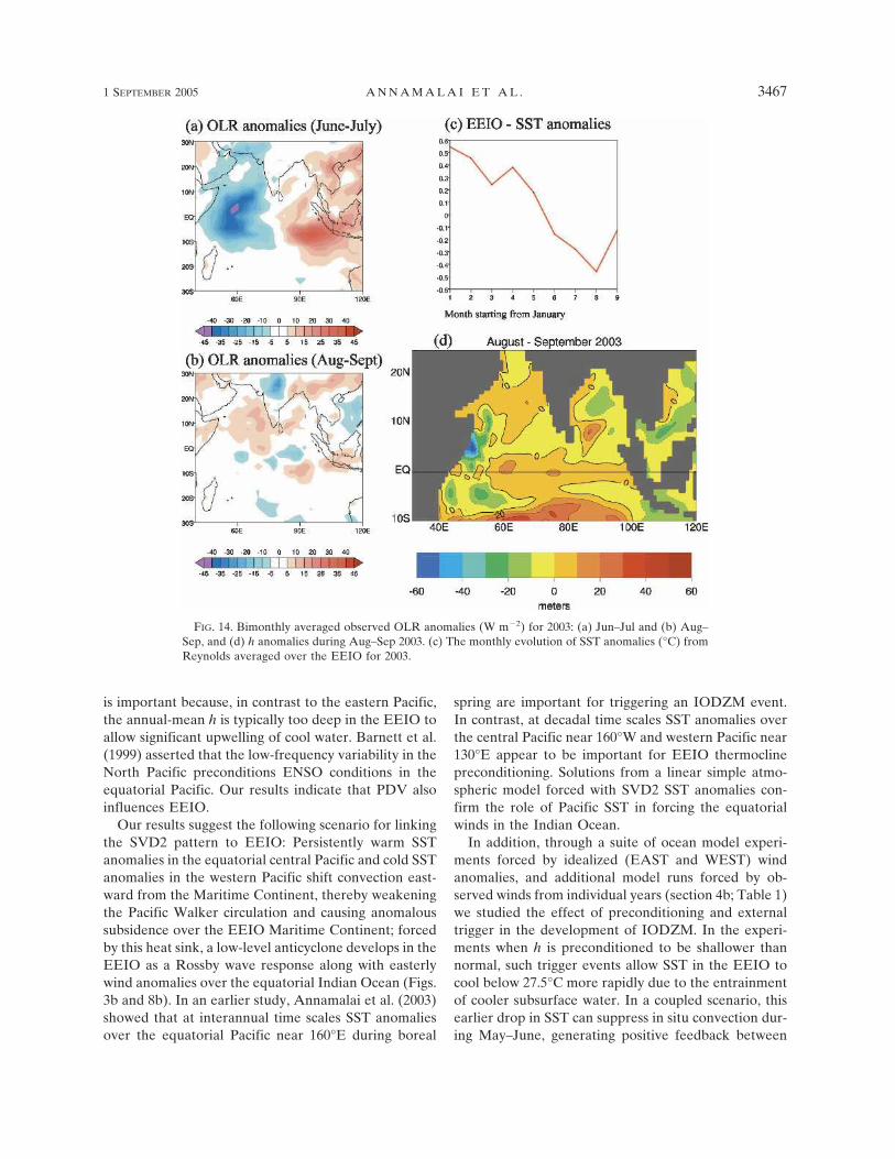
(Fig. 14). The anomalous SST evolution over the EEIOduring 2003 (Fig. 14c) shows that the cooling duringJune–July is accompanied by weakened convection andanomalous equatorial easterlies over the Indian Ocean(Fig. 14a). In sharp contrast, h over the EEIO is deeperthan normal in August (Fig. 14d). As a result, the cool-ing vanished by mid-August (Fig. 14c) and anomalousconvection strengthened over the EEIO (Fig. 14b) ter-minating the development of the IODZM event. Amixed-layer heat budget analysis for 2003 (not shown)indicates that SST cooling was primarily due to wind-driven fluxes with little contribution from the entrain-ment term.

5. Discussion and summary

In the present study, we explore the hypothesis thatPDV is an important factor in determining the occur-rence of strong IODZM events in the 1960s and 1990s,through both atmospheric teleconnections to the IndianOcean equatorial wind field and oceanic teleconnec-tions via the Indonesian Throughflow. In the presentstudy, however, more focus has been paid to the role ofthe atmospheric teleconnection.

To identify the influence of PDV in the Indo-Pacificdomain, we performed SVD analysis on low-pass-filtered data (section 3a). The SST pattern of SVD1captures the traditional PDV pattern, and the surfacewinds show weakening of the easterly trade winds in

the Pacific, implying El Niño–like conditions. The hanomalies in the Indian Ocean are shallower than nor-mal off south Java (Fig. 2c). The strong phase relation-ship between PC1 of h (Fig. 4a) and the 8-yr runningmean of ITF (Fig. 4c) indicates that SVD1 influencesthe EEIO thermocline primarily due to a reduction inthe ITF transport. The PC1 of all these variables cap-ture the major climate shift of 1976–77. We note thatSVD1 contribution to the overall EEIO thermoclinepreconditioning is rather small.

The SVD2 patterns are new findings of the presentstudy (Fig. 3). The SST pattern of SVD2 captures thecooling (warming) over the western (central) Pacificduring 1952–71 and 1989–96. The associated surfacewind variability captures easterly wind anomalies overthe equatorial Indian Ocean together with anticycloniccirculation anomalies in the southeastern IndianOcean. The known oceanic response to this wind patchis to shoal the EEIO thermocline (Fig. 3c). Collectively,SVD1 and SVD2 are referred to as PDV in the presentstudy. A separate SVD analysis with Indian Ocean SSTreveals negligible impact on EEIO thermocline (Fig. 5).

Based upon the two PCs we define an index, I, thatmeasures h in the EEIO (section 3b). Consistent withthe hypothesis, I indicates shallower-than-normal hduring 1958–69 and 1990–96 (Fig. 6). This hypothesisallows for the growth of a coupled mode in the EEIO inthe absence of ENSO forcing given appropriate pre-conditioning of the thermocline. Such preconditioning

FIG. 13. Same as in Fig. 11 but for (a) EAST96 (blue) and WEST96 (red) and (b) EAST57(blue) and WEST57 (red). The 27.5°C threshold required for deep convection to occur in theTropics is shown as dotted line.


Fig 13 live 4/C

is important because, in contrast to the eastern Pacific,the annual-mean h is typically too deep in the EEIO toallow significant upwelling of cool water. Barnett et al.(1999) asserted that the low-frequency variability in theNorth Pacific preconditions ENSO conditions in theequatorial Pacific. Our results indicate that PDV alsoinfluences EEIO.

Our results suggest the following scenario for linkingthe SVD2 pattern to EEIO: Persistently warm SSTanomalies in the equatorial central Pacific and cold SSTanomalies in the western Pacific shift convection east-ward from the Maritime Continent, thereby weakeningthe Pacific Walker circulation and causing anomaloussubsidence over the EEIO Maritime Continent; forcedby this heat sink, a low-level anticyclone develops in theEEIO as a Rossby wave response along with easterlywind anomalies over the equatorial Indian Ocean (Figs.3b and 8b). In an earlier study, Annamalai et al. (2003)showed that at interannual time scales SST anomaliesover the equatorial Pacific near 160°E during boreal

spring are important for triggering an IODZM event.In contrast, at decadal time scales SST anomalies overthe central Pacific near 160°W and western Pacific near130°E appear to be important for EEIO thermoclinepreconditioning. Solutions from a linear simple atmo-spheric model forced with SVD2 SST anomalies con-firm the role of Pacific SST in forcing the equatorialwinds in the Indian Ocean.

In addition, through a suite of ocean model experi-ments forced by idealized (EAST and WEST) windanomalies, and additional model runs forced by ob-served winds from individual years (section 4b; Table 1)we studied the effect of preconditioning and externaltrigger in the development of IODZM. In the experi-ments when h is preconditioned to be shallower thannormal, such trigger events allow SST in the EEIO tocool below 27.5°C more rapidly due to the entrainmentof cooler subsurface water. In a coupled scenario, thisearlier drop in SST can suppress in situ convection dur-ing May–June, generating positive feedback between

FIG. 14. Bimonthly averaged observed OLR anomalies (W m�2) for 2003: (a) Jun–Jul and (b) Aug–Sep, and (d) h anomalies during Aug–Sep 2003. (c) The monthly evolution of SST anomalies (°C) fromReynolds averaged over the EEIO for 2003.


Fig 14 live 4/C

the ocean and atmosphere that can lead to a strongIODZM event. Conversely, an IODZM event does notdevelop when h is anomalously deep. The proposedconceptual picture is evident during the evolution of aweak IODZM event that occurred in the summer of2003. In summary, the difference between all EASTand WEST experiments is merely the timing of the ap-pearance of the 27.5°C isotherm to perturb the overly-ing atmospheric precipitation.

In conclusion, we have presented evidence indicatingthat a shallow thermocline in the EEIO is a necessaryprecondition for strong IODZM activity. However,there are caveats that temper our results. First, the re-gions off Java and Sumatra are data void, and thereforethe SST analysis prior to the satellite era is debatable.Sustained observational efforts, by both in situ andspace-borne sensors, are necessary to confirm the pre-ferred occurrence of strong IODZM events in certaindecades. Second, our supporting numerical experimentutilizes an ocean model forced by observed winds,whereas the winds themselves are end products ofcoupled ocean–atmosphere processes. Our hypothesis,then, remains to be confirmed in a coupled model thatinternally develops its own winds, and efforts are cur-rently under way to achieve this goal.

Acknowledgments. The authors thank Dr. NiklasSchneider for fruitful discussions and for comments onan earlier version of the manuscript. Dr. Axel Timmer-mann is thanked for suggesting the statistical signifi-cance test used to prepare Fig. 7. This research wassupported by the Japan Agency for Marine-Earth Sci-ence and Technology (JAMSTEC) through its sponsor-ship of the International Pacific Research Center. R.Murtugudde acknowledges NASA Indian Ocean Bio-geochemistry, ISO, Salinity, and TRMM grants for par-tial support during this work. Partial support from theNOAA/OGP/Pacific program is also acknowledged.The comments and critics from the anonymous review-ers are greatly appreciated.

REFERENCES

Alan, R. J., and Coauthors, 2001: Is there an Indian Ocean dipole,and is it independent of the El Niño–Southern Oscillations?CLIVAR Exchanges, Vol. 6, No. 3, 18–22.

Annamalai, H., J. M. Slingo, K. R. Sperber, and K. Hodges, 1999:The mean evolution and variability of the Asian summermonsoon: Comparison of ECMWF and NCEP–NCAR re-analyses. Mon. Wea. Rev., 127, 1157–1186.

——, R. Murtugudde, J. Potemra, S. P. Xie, P. Liu, and B. Wang,2003: Coupled dynamics in the Indian Ocean: Spring initia-tion of the zonal mode. Deep-Sea Res., 50B, 2305–2330.

Barnett, T. P., D. W. Pierce, M. Latif, D. Dommenget, and R.Saravanan, 1999: Interdecadal interactions between the trop-

ics and midlatitudes in the Pacific basin. Geophys. Res. Lett.,26, 615–619.

Behera, S. K., R. Krishnan, and T. Yamagata, 1999: Unusualocean-atmosphere conditions in the tropical Indian Oceanduring 1994. Geophys. Res. Lett., 26, 3001–3004.

Betts, A., and M. J. Miller, 1986: A new convective adjustmentscheme. Part II: Single column tests using GATE wave,BOMEX, ATEX, and artic air-mass data sets. Quart. J. Roy.Meteor. Soc., 112, 693–709.

Bjerknes, J., 1969: Atmospheric teleconnections from the equa-torial Pacific. Mon. Wea. Rev., 97, 163–172.

Bretherton, C. S., A. Smith, and J. M. Wallace, 1992: An inter-comparison of methods for finding coupled patterns in cli-mate data. J. Climate, 5, 541–560.

Chen, D., L. M. Rothstein, and A. J. Busalacchi, 1994: A hybridvertical mixing scheme and its application to tropical oceanmodels. J. Phys. Oceanogr., 24, 2156–2179.

Deser, C., A. S. Phillips, and J. W. Hurrell, 2004: Pacific interdec-adal climate variability: Linkages between the Tropics andthe North Pacific during boreal winter since 1900. J. Climate,17, 3109–3124.

Feng, M., and G. Meyers, 2003: Interannual variability in thetropical Indian Ocean: A two-year time-scale of the IndianOcean Dipole. Deep-Sea Res., 50B, 2263–2284.

Graham, N. E., and T. P. Barnett, 1987: Sea surface temperature,surface wind divergence, and convection over tropicaloceans. Science, 258, 657–659.

Gill, A. E., 1980: Some simple solutions for heat induced tropicalcirculation. Quart. J. Roy. Meteor. Soc., 106, 447–462.

Hackert, E., A. J. Busalacchi, and R. Murtugudde, 2001: A windcomparison study using an ocean general circulation modelfor the 1997–98 El Niño. J. Geophys. Res., 106, 2345–2362.

Hare, S. R., and N. J. Mantua, 2000: Empirical evidence for NorthPacific regime shifts in 1977 and 1989. Progress in Oceanog-raphy, Vol. 47, Pergamon, 103–145.

Hastenrath, S., 2002: Dipoles, temperature gradients, and tropicalclimate anomalies. Bull. Amer. Meteor. Soc., 83, 735–738.

Huang, B., and J. L. Kinter, 2002: The interannual variability inthe tropical Indian Ocean and its relations to El Niño–Southern Oscillation. J. Geophys. Res., 107, 3199,doi:10.1029/2001JC001278.

Kalnay, E., and Coauthors, 1996: The NCEP/NCAR 40-Year Re-analysis Project. Bull. Amer. Meteor. Soc., 77, 437–471.

Kinter, J. L., M. J. Fennessy, V. Krishnamurthy, and L. Marx,2004: An evaluation of the apparent interdecadal shift in thetropical divergent circulation in the NCEP–NCAR reanaly-sis. J. Climate, 17, 349–361.

Krishnamurthy, V., and B. Kirtman, 2003: Variability of the In-dian Ocean: Relation to monsoon and ENSO. Quart. J. Roy.Meteor. Soc., 129, 1623–1646.

Latif, M., and T. Barnett, 1994: Causes of decadal variability overthe North Pacific and North America. Science, 266, 634–637.

Levitus, S., and T. Boyer, 1994: Temperature. Vol. 4, World OceanAtlas 1994, NOAA Atlas NESDIS 4, 117 pp.

McPhaden, M., and D. Zhang, 2004: Pacific Ocean circulationrebounds. Geophys. Res. Lett., 31, L18301, doi:10.1029/2004GL020727.

Meyers, G., 1996: Variation of Indonesian throughflow and the ElNiño–Southern Oscillation. J. Geophys. Res., 101, 12 255–12 263.

Minobe, S., 1997: A 50–70 year climatic oscillation over the NorthPacific and North America. Geophys. Res. Lett., 24, 683–686.

Murtugudde, R., and A. J. Busalacchi, 1999: Interannual variabil-


ity of the dynamics and thermodynamics of the tropical In-dian Ocean. J. Climate, 12, 2300–2326.

——, ——, and J. Beauchamp, 1998a: Seasonal to interannualeffects of the Indonesian Throughflow on the tropical Indo-Pacific basin. J. Geophys. Res., 103, 21 425–21 441.

——, B. N. Goswami, and A. J. Busalacchi, 1998b: Air-sea inter-action in the southern tropical Indian Ocean and its relationsto interannual variability of the monsoon over India. Proc.Int. Conf. on Monsoon and Hydrologic Cycle, Kyongju, Ko-rea, Korean Meteorological Agency, 184–188.

——, J. P. McCreary, and A. J. Busalacchi, 2000: Oceanic pro-cesses associated with anomalous events in the Indian Oceanwith relevance to 1997–1998. J. Geophys. Res., 105, 3295–3306.

Nakamura, H., and T. Yamagata, 1999: Recent decadal SST vari-ability in the Northwestern Pacific and associated atmo-spheric anomalies. Beyond El Niño: Decadal and Interdec-adal Variability, A. Navarra, Ed., Springer, 49–72.

——, G. Lin, and T. Yamagata, 1997: Decadal climate variabilityin the North Pacific during recent decades. Bull. Amer. Me-teor. Soc., 78, 2215–2225.

Nitta, T., and S. Yamada, 1989: Recent warming of tropical seasurface temperature and its relationship to the NorthernHemisphere circulation. J. Meteor. Soc. Japan, 67, 375–383.

Pierce, D. W., T. P. Barnett, and M. Latif, 2000: Connection be-tween the Pacific Ocean Tropics and midlatitudes on decadaltime scales. J. Climate, 13, 1173–1194.

Potemra, J. T., S. L. Hautala, J. Sprintall, and W. Pandoe, 2003:Vertical structure of Indonesian throughflow in a large-scalemodel. Deep-Sea Res., 50, 2143–2162.

Rao, S. A., S. K. Behera, Y. Masumoto, and T. Yamagata, 2002:Interannual subsurface variability in the tropical IndianOcean with a special emphasis on the Indian Ocean dipole.Deep Sea Res., 49B, 1549–1572.

Rayner, N. A., D. E. Parker, E. B. Horton, C. K. Folland, L. V.Alexander, D. P. Rowell, E. C. Kent, and A. Kaplan, 2003:Global analyses of sea surface temperature, sea ice, and nightmarine air temperature since the late nineteenth century. J.Geophys. Res., 108, 4407, doi:10.1029/2002JD002670.

Reppin, J., F. A. Schott, J. Fisher, and D. Quadfasel, 1999: Equa-torial currents and transports in the upper central IndianOcean: Annual cycle and interannual variability. J. Geophys.Res., 104, 15 495–15 514.

Reverdin, G., D. Cadet, and D. Gutzler, 1986: Interannual dis-placements of convection and surface circulation over theequatorial Indian Ocean. Quart. J. Roy. Meteor. Soc., 112,43–46.

Reynolds, R. W., and T. M. Smith, 1994: Improved global sea sur-face temperature analyses using optimal interpolation. J. Cli-mate, 7, 929–948.

Saji, N. H., B. N. Goswami, P. N. Vinayachandran, and T. Yama-gata, 1999: A dipole mode in the tropical Indian Ocean. Na-ture, 401, 360–363.

Schneider, N., A. J. Miller, and D. W. Pierce, 2002: Anatomy ofNorth Pacific decadal variability. J. Climate, 15, 586–605.

Schreiber, T., and A. Schmitz, 1996: Improved surrogate data fornonlinearity tests. Phys. Rev. Lett., 77, 635–638.

Simmons, A. J., and Coauthors, 2004: Comparison of trends andvariability in CRU, ERA-40 and NCEP-NCAR analyses ofmonthly-mean surface air temperature. ERA_40 ProjectReport Series 18, 42 pp. [Available online at http://www.ecmwf.int/publications.]

Smith, T. M., and R. W. Reynolds, 2004: Improved extended re-construction of SST (1854–1997). J. Climate, 17, 2466–2477.

Solomon, A., J. P. McCreary, R. Kleeman, and B. Klinger, 2003:Interannual and decadal variability in an intermediatecoupled model of the Pacific region. J. Climate, 16, 383–405.

Susanto, R. D., A. L. Gordon, and Q. Zheng, 2001: Upwellingalong the coasts of Java and Sumatra and its relation toENSO. Geophys. Res. Lett., 28, 1599–1602.

Vinaychandran, P. N., N. H. Saji, and T. Yamagata, 1999: Re-sponse of the equatorial Indian Ocean to an unusual windevent during 1994. Geophys. Res. Lett., 26, 1613–1616.

Watanabe, M., and M. Kimoto, 2000: Atmosphere–ocean thermalcoupling in the North Atlantic: A positive feedback. Quart. J.Roy. Meteor. Soc., 126, 3343–3369.

——, and F. F. Jin, 2003: A moist linear baroclinic model:Coupled dynamical–convective response to El Niño. J. Cli-mate, 16, 1121–1139.

Webster, P. J., A. M. Moore, J. P. Loschnigg, and R. R. Leben,1999: Coupled oceanic–atmospheric dynamics in the IndianOcean during 1997–98. Nature, 401, 356–360.

Xie, P., and P. Arkin, 1996: Analyses of global monthly precipi-tation using gauge observations, satellite estimates, and nu-merical model predictions. J. Climate, 9, 840–858.

——, H. Annamalai, F. A. Schott, and J. P. McCreary, 2002:Structure and mechanisms of south Indian Ocean climatevariability. J. Climate, 15, 867–878.

Yamagata, T., S. Behera, S. A. Rao, Z. Guan, K. Ashok, andN. H. Saji, 2003: Comments on “Dipoles, temperature gradi-ent, and tropical climate anomalies.” Bull. Amer. Meteor.Soc., 84, 1418–1422.

Yu, L., and M. Rienecker, 1999: Mechanisms for the Indian Oceanwarming during the 1997–98 El Niño. Geophys. Res. Lett., 26,735–738.

——, and ——, 2000: Indian Ocean warming of 1997–1998. J.Geophys. Res., 105, 16 923–16 939.

Zhang, Y., J. M. Wallace, and D. Battisti, 1997: ENSO-like inter-decadal variability: 1990–93. J. Climate, 10, 1004–1020.


Documents

Effect of Preconditioning on the Extreme Climate …iprc.soest.hawaii.edu/users/jimp/papers/iozm_idec.pdf · Effect of Preconditioning on the Extreme Climate Events in the Tropical