Embed Size (px)
Citation preview
Western Michigan University Western Michigan University
ScholarWorks at WMU ScholarWorks at WMU
Dissertations Graduate College
12-1987
Effect of Polymerization Conversion on the Experimental Effect of Polymerization Conversion on the Experimental
Determination of Monomer Reactivity Ratios in Copolymerization Determination of Monomer Reactivity Ratios in Copolymerization
Sevim Zeynep Erhan Western Michigan University
Follow this and additional works at: https://scholarworks.wmich.edu/dissertations
Part of the Chemistry Commons
Recommended Citation Recommended Citation Erhan, Sevim Zeynep, "Effect of Polymerization Conversion on the Experimental Determination of Monomer Reactivity Ratios in Copolymerization" (1987). Dissertations. 3438. https://scholarworks.wmich.edu/dissertations/3438
This Dissertation-Open Access is brought to you for free and open access by the Graduate College at ScholarWorks at WMU. It has been accepted for inclusion in Dissertations by an authorized administrator of ScholarWorks at WMU. For more information, please contact [email protected].

EFFECT OF POLYMERIZATION CONVERSION ON THE EXPERIMENTAL DETERMINATION OF MONOMER REACTIVITY
RATIOS IN COPOLYMERIZATION
by
Sevim Zeynep Erhan
A Dissertation
Submitted to the
Faculty of The Graduate College
in partial fulfillment of the
requirements for the
Degree of Doctor of Philosophy
Department of Chemistry
Western Michigan University
Kalamazoo, Michigan
December 1987

To Dr. G. G. Lowry
and Dr. R. C. Nagler

ACKNOWLEDGEMENTS
I wish to express my sincere appreciation to Dr. G. G. Lowry for
his patience and assistance during the course.of this investigation.
His helpful suggestions and critical eye were invaluable and greatly
appreciated.
I also wish to acknowledge Dr. J. A. Howell, who was extremely
helpful and prov�ded much advice with respect to spectroscopic
experimental techniques.
I wish to express my appreciation to all the committee members
who have contributed to this work, and my friend Bulent Acar for his
help in mathematical problems.
I would like to thank the Chemistry Department of Western
Michigan University for the financial aid and teaching experience
gained from my teaching assistantship.
Finally, I want to express my gratitude to my husband for his
many sacrifices and assistance in preparing this manuscript and.for
his support during the course of my studies.
Sevim Zeynep Erhan
ii

EFFECT OF POLYMERIZATION CONVERSION ON THE EXPERIMENTAL
DETERMINATION OF MONOMER REACTIVITY
RATIOS IN COPOLYMERIZATION
Sevim Zeynep Erhan, Ph.D.
Western Michigan University, 1987
In this study the comparison of the methods used to calculate
monomer reactivity ratios from experimental copolymer composition
data is targeted. -
For this purpose, nine samples of each of nine different
concentrations of styrene-methyl methacrylate monomer mixtures were
prepared. These mixtures were then polymerized for different times
ranging from one to nine hours and the percent conversion to
copolymer was determined.
The compositions of these copolymers were determined by their
refractive index increments measured in two different solvents.
Ultraviolet absorption spectroscopy was also studied as a possible
method to fi.nd copolymer compositions. Though this method has been
used previously, UV absorption by copolymers appears to be related
to monomer sequence so that a simple application of Beer's Law is
not valid.
As the best method to calculate r1 and r2 values, the Maximum
Likelihood Method was taken. This method gave r1=0.495 and r2=0.467
where styrene is monomer 1. These values were then compared to the

r1 and r2 values obtained from a Nonlinear Least Squares Method,
Intersection Method, Fineman-Ross Method and the Kelen-Tudos Method.
From this comparison it was seen that the Nonlinear Least Squares
Method gave the best results. The Intersection Method gave better
results than the Kelen-Tudos Method which in turn was better than
the Fineman-Ross Method. Also it was observed that the calculation
method of Fineman-Ross led to inconsistent monomer reactivity
ratios.
This study iJ concluded with recommendations for further
research in the area of penultimate effect in propagation,
copolymers using monomers that will give a larger composition drift,
and studies on the method of UV analysis of copolymer compositions
taking the absorption of methyl methacrylate into consideration.

ACKNOWLEDGEMENTS
LIST OF TABLES
LIST OF FIGURES
CHAPTER
I • INTRODUCTION
TABLE OF CONTENTS
Theory of Free Radical Copolymerization
Copolymer Composition Analysis
Elemental and Functional Group Analysis
Specttoscopic Analysis
Ultraviolet Spectroscopy
Infrared Spectroscopy
Nuclear Magnetic Resonance Spectroscopy
Visible Spectroscopy
Differential Refractometry
Methods of Determining r1 and r2 Values
Direct-Curve Fitting on Polymer-Monomer Composition Plots • . . .
Intersecting Slopes Method
.Fineman and Ross Method
Kelen and Tudos Method
Quantitative Treatment of Composition Drift
Goals of Current Research
II. EXPERIMENTAL
Preparation of Low Conversion StyreneMethylmethacrylate Copolymers
Purification of Copolymers
iii
ii
V
vi
1
1
4
4
5
6
8
9
11
11
15
15
16
16
17
18
22
24
24
25

Table of Contents -- Continued
CHAPTER
Determination of Copolymer Composition 26
Method of Obtaining Refractive Index Increments 26
UV Absorption Spectra of Copolymers
III. RESULTS AND DISCUSSION
28
29
29 Results of Conversion Studies
Copolymer Composition Studies with Refractive Index Increments Measurements • . • • •
Evaluation of Methods of Estimating Monomer Reactivity Ratios From Experimental Data
Maximum Likelihood Method
I
Methods Using Extrapolated Zero-Conversion Data
Non-Linear Least Squares
· Intersection Method
Fineman and Ross Method
Kelen and Tudos Method
30
32
32
38
41
41
48
52
Effect of Composition Drift With Conversion 52
Comparison of Methods and Discussion 54
Analysis of Ultraviolet Absorption Spectra of Styrene-. Me�hyl Methacrylate Copolymer • • • • 61
Conclusions
Recommendations
APPENDICES
68
69
70
A. Experimental Data for Copolymerizationof Styrene With Methyl Methacrylate • • • . • . . . • .
B. Calculated Values of Composition andConversion for Copolymerization ofStyrene With Methyl Methacrylate
REFERENCES
iv
71
82
94
LIST OF TABLES
1. Copolymer Composition Data Using Weighted Nonlinear
Least Squares • . • . . • . . . . . • . • 41
2. Monomer Reactivity Ratios and Uncertainties
at Each Intersection Point . • . . • . 45
3. Comparison of Methods 55
4. Experimental Values of Styrene-Methyl Methacrylate
Copolymers . . . . . . . . . . . . . . . . . . . 67
V

1.
2.
3.
4.
5.
LIST OF FIGURES
Schematic Diagram of the Working Principle of a
Brice-Phoenix Visual Differential Refractometer
Diagram of the Cell of a Brice-Phoenix Visual Differential Refractometer • . . • • • • • •
Rate of Copolymerization of Styrene and Methyl Methacrylate, in mole percent per hour, at 60.0 ±0.1°C, Horizontal bars Represent Standard Error of Estimate . . • • .
Contours Representing Surface of Residuals - Squared for Nonlinear Least Squares Fitting of Weighted Styrene-Methyl Methacrylate Copolymer Data. Points Represent Different Methods of Evaluation, Maximum Likelihood (�), Nonlinear Least Squares (0), Intersection(□), Kelen-Tudos (◊), Fineman-Ross (V)
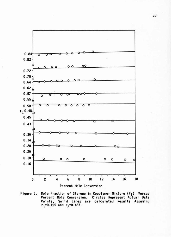
Mole Fraction of Styrene in Copolymer Mixture (F1) versus Percent Mole Conversion. Circles Represent Actual Data Points, Solid Lines are Calculated Results Assuming r1=0,495 and r2=0.467
6. Illustration of the Application of the IntersectionMethod to the Data of Table 1. The Values on theGraph are Approximate Monomer Compositions,Actual Compositions are Given in Table 1
7. a: Fineman-Ross Method Using Equation 1. 19, Styrene as Monomer 1 . . . . . . . . . . . .
b: Fineman-Ross Method Using Equation 1.19, Methyl Methacrylate as Monomer 1 . . . . .
8. a: Fineman-Ross Method Using Equation 1.20,Styrene as Monomer 1 . . . . . . . . . . . .
b: Fineman-Ross Method Using Equation 1.20, Methyl Methacrylate as Monomer 1 . . . .
9. a: Kelen-Tudos Method, Styrene as Monomer 1
b: Kelen-Tudos Method, Methyl Methacrylate as Monomer
. .
. .
. .
1
10. Instantaneous Composition of Copolymer, F1 as a Functionof Monomer Composition f1 for the Values of ReactivityRatios, r1 and r2, 0.495 and 0.467. Circles
vi
13
13
31
37
39
42
49
49
51
51
53
53

List of Figures -- Continued
Represent Copolymer Composition Extrapolated to Zero Conversion, Solid Line is Calculated Value • • • 56
11. Analysis of Residuals from Nonlinear Least SquaresFitting. Lines Represent 95% Confidence Limits . . • . 60
12. UV Absorption of Styrene-Methyl Methacrylate Copolymer.Solid Line Represents Non-Linear Least Squares FittedCurves Assuming Three Chromophores of Styrene Units.Dashed Line Represents Simple Beer's Law Curve 63
13. Overlapped Ultraviolet Absorption Spectrum of the VariousMonomer Feed Compositions of Styrene-Methyl MethacrylateCopolymers all Containing l.0mg/mL of Styrene • . • • 64
14. A Theoretical Plot of Triad Compositions as a Function ofMonomer Compositions when r1=0.495 and r2=0.467 • . • . 66
vii

CHAPTER I
INTRODUCTION
Theory of Free Radical Copolymerization
In free radical copolymerization as in ordinary free radical
homopolymerization, the simple mechanistic chain reactions which
lead to the formation of a polymer molecule consist of three steps:
initiation, propagation, and termination. The chemical composition
of high molecular weight copolymers is dependent as a first
approximation only.on the propagation of the chain reaction.
If one of the monomers in a copolymer is designated M1 and the
other M2, it can be shown that if the addition of these monomers of
the growing radical were dependent on the makeup of the entire
polymer radical, then an infinite number of different reaction rates
would occur since the process would depend on both chain length and
detailed composition. It was postulated as early as 1936 by Dostal1
that the kinetic behavior of the chain radical was dependent only on
the terminal group (the monomer unit last added to the growing
chain) and that the kinetic behavior was independent of the length
or over-all composition of the polymer chain.
Under these conditions the composition of the copolymer chain
is determined by the following four propagation reactions:
Growing Adding Chain Monomer
� ml. + M
l � m1m1• (1.1)
� ml. + M
2� m1m2• ( 1. 2)
� m2•+ M
2� m2m2• ( 1. 3)
� m2•+ M
l � m2m1• (1.4)
l
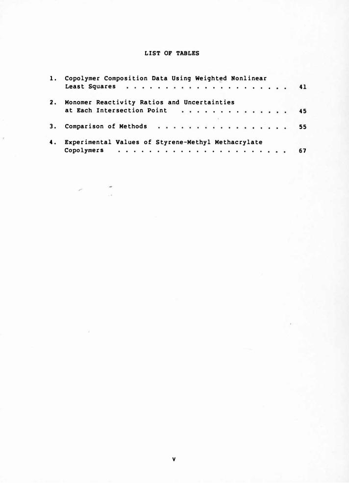
The rates of these reactions are written as
d [M1] = k11 [m1 •] [M1]
dt (1. 5)
d [M2] k12 [m1 •] [M2] dt
(1. 6)
d [M2] k22 [m2•J [M2] =
dt ( l. 7}
d[M1] = k21 [m2 •] [M1]
dt ( l. 8)
Dostal was able to write correct mathematical expressions for
the rate of copol1merization and the composition of a copolymer in
terms of these rates, but since four unknown rate constants were
involved he could not devise any experimental tests for his
conclusions.
Wall in 19412 showed that the chemical composition of
copolymers was dependent only on the relative reactivities of the
two monomers to the two radicals. Be expressed these relative
reactivities in the form of ratios r1 and r2, called "monomer
reactivity ratios," which he defined as follows:
= and
Mayo and Lewis3 in a classic work undertook a systematic study
of copolymerization and arrived at the following rate expressions
for the consumption of monomers M1 and M2, considering only the
propagation reactions: d [M1J
(1.9) dt
(1. 10)
dt
2

In the steady state of copolymerization, concentrations of
different types of free radicals must be maintained constant.
This means that in the steady state the rate at which [m1 •) is
destroyed is equal to the rate at which [m2 •) is destroyed. It is
then possible to solve for the concentration of one of the radicals
in the steady state in terms of the other. Mayo and Lewis applied
this steady state assumption to the ratio of the rates of
disappearance of the two monomers and arrived at the following
relation:
d[M1)(1.11)
d [M2]
Using the definition of monomer reactivity ratios defined by
Wall, this can be simplified to
= (::::) r1 [M1) + [M2]
r2 [M2) + [M1] (1. 12)
It is evident that the ratio of the rates of consumption of the
two monomers ,is also the ratio of molar concentrations of structural
uni ts derived from the two monomers in the copolymer. Defining the
instantaneous concentration of monomer M1 in the copolymer as "mi"
and the concentration of monomer M2 in the copolymer as "m2" then;
r1 [M1) + [M2)
r2 [M2) + [M1) (1.13)
3

This equation is known as the "Copolymer Composition Equation".
This same equation was derived independently by Alfrey and
Goldfinger4 at approximately the same time using the same reasoning.
The copolymer composition equation has been used to predict the
average composition of the polymer formed at any instant in the
polymerization when the relative concentrations of monomers are
known and the values of the monomer reactivity ratios are either
known or assumed. It has also been used to calculate the values of
the monomer reactivity ratios, r1 and r2' from experimental data
including the known relative concentrations of monomers and the
composition of the copolymer formed. The experimental technique
that is normally used' consists of preparing a series of the
copolymers for various M1 and M2 monomer concentrations and analyz
ing the resulting copolymers for the concentrations of "m1" and "m2"
they contain. The conversion of the monomer to copolymer in this
series must be kept low because equation (1.13) is valid only
for instantaneous copolymerization, and the assumption is made
that low conversion copolymerization approximates instantaneous
copolymerization.
Copolymer Composition Analysis
Elemental and Functional Group Analysis
The average copolymer composition can be determined by a
variety of techniques including elemental and other chemical
analysis. Elemental analysis is a popular method and copolymer
4

compositions obtained from this technique are often used to
calibrate or compare with results from other techniques3. However,
uncertainty as to the completeness of combustion during elemental
analysis leads to uncertainty in the final results. This can be
minimized by submitting samples of the M1 & .M2 homopolymers to the
analyst along with the copolymer samples. Automatic commercial
analyzers exist which determine the carbon and hydrogen content of
copolymers by combustion of the samples. Oxygen content is usually
determined by difference. Also in organic compounds nitrogen is
determined by Kjeldahl and Dumas methods, oxygen by neutron
activation and halogens by sodium fusion.
Copolymers can also be analyzed chemically for the existence of
particular functional groups. However, problems can arise due to
the low solubility of copolymers or inaccessibility of functional
groups5. Unique chemical procedures which are very accurate have
been developed for some specific copolymers.
Spectroscopic Analysis
When a beam of electromagnetic radiation is transmitted through
a copolymer sample it may, depending on the wavelength, A, be
partially absorbed. Absorption processes are generally associated
with some form of transition of the molecule or portion of the
molecule between two energy states. The difference in energy, AE,
between the two energy states is a function of the wavelength,
AE = h•c/A, where h is Planck's constant and c is speed of light in
vacuum.
5

Copolymers, as well as all other molecules, exhibit various
absorption mechanisms, each characterized by a different AE, and
thus absorption may be observed at several different wavelengths or
wavelength regions. Four regions of the electromagnetic spectrum
have been traditionally used to probe copolymers and molecules in
general:
regions.
the ultraviolet, visible, infrared and radio-frequency
Ultraviolet Spectroscopy
The absorption of UV radiation is associated with the
excitation of electrons
state.
aromatic
Specific
groups)
groups
from a ground state to a higher energy
or chromophores (such as carbonyl or
generally absorb UV radiation at specific
wavelengths and have nearly the same molar absorptivity in many
different molecules.
The determination of copolymer composition by UV spectroscopy
would seem to be a simple matter, providing one monomer contains a
UV absorbing chromophore and the other does not. Since styrene
absorbs strongly in the UV, the determination of the styrene content
in copolymers has been a popular method of analysis6-14.
In the use of UV spectroscopy to determine copolymer
composition it is assumed that Beer's Law is valid, or a linear
relationship exists between the observed absorption, A, and the
(1.14)
concentration of the UV absorbing chromophore, c, where C1 is the
absorptivity and b is the path length of the cell.
6

Unfortunately the UV analysis of poly (styrene-methylmetha
crylate) copolymer [poly (sty-co-mma)] has indicated that Beer's
Law, eq. (1.14), does not seem to hold7 -13. The observed
hypochromism of poly ( sty-co-mma) solutions has been assumed to be
due to variations in microstructure or con_formational changes in
solution. O'Driscoll et al. 8 rationalized the ideal absorption
behavior in terms of styrene dyads, while Stutzel et al. 12 proposed
a model based on styrene triads. Gall and Russo10• 11 observed
hypochromic effects over a specific copolymer composition range
which varied with the solvent used, which suggested changes in
conformation of the macromolecules in solution.
In spite of the evidence outlined above, UV spectroscopy has
been used to analyze poly (sty-co-mma) assuming Beer's Law was
applicable8• 15• 16.
Recently Garcia-Rubio17 has critically assessed the UV
literature data on a variety of styrene copolymers and suggested
that eq. (1.14) is not valid since the phenyl ring of styrene is not
the only UV absorbing chromophore.
relationship was derived:
The following empirical
£c (l.) = £ps (l.) • P1w + £i (l.) • (l-P1w) (1.15)
In equation (1.15), ec (l.) is the copolymer absorptivity at
wavelength l., £ps ( l.) is polystyrene absorptivity, P1w is weight
fraction of styrene in the copolymer, £i (l.) is the comonomer
absorptivity.
7

In conclusion, UV spectral analysis and Beer's Law can be
applied to copolymers providing all the chromophores can be
identified, although identification of all chromophores is a
difficult problem. It may be possible to obtain reliable copolymer
composition data from UV provided the data are treated properly.
Infrared Spectroscopy
Infrared spectroscopy is one of the techniques used to identify
polymers and copolymers. IR spectroscopy, or vibrational
spectroscopy invo�ves the variation of intermolecular distances, or
molecular vibration. As an example, in a heteronuclear diatomic
molecule, with only one vibrational degree of freedom, there is a
fundamental frequency at which the bond stretches. The stretching
or oscillating of the diatomic molecule results in an oscillating
electric dipole which will interact with the oscillating electric
field of light, if this light has the proper infrared frequency.
Interaction results in the absorption of the IR radiation and the
diatomic molecule undergoes a transition to a higher vibrational
energy level. More detailed explanations can be found in Colthup et
al.18.
In more complex molecules containing N atoms, there will be
JN-6 or 3N-5 (if linear molecule} fundamental vibrations, thus it
would appear polymer spectra would be extremely complex.
Fortunately, µ�m of side group for many fundamental vibrations, and
it is possible to assign IR absorption frequencies to particular
vibrating bonds, functional groups or groups of atoms. The
absorptions observed in the IR spectra19 and Raman spectra (which
8

involve rotational transitions)2D of complex molecules have been
tabulated and assigned to various organic and inorganic functional
groups.
The IR spectrum of a polymer is commonly obtained from a thin
film (occasionally solutions are used). Quantitative IR investiga
tions have been rare, since this requires knowledge of the
absorptivity of the band or peak observed and of the thickness of
the sample. Accurate absorptivi ties can be obtained from model
compounds. However for solid sample the thickness of the sample is
difficult to measure with good accuracy and since the film is so
thin, errors in the measurement of film thickness result in very
large composition errors. In the IR spectra of polymer films, an
interference pattern is often seen, from which film thickness may be
calculated, or at least estimated.
Another problem can arise if the polymer chains in the film are
oriented, since Beer's Law assumes a random orientation21• Thus,
IR-absorbing groups may be anisotropic in oriented polymers so that
absorbance depends on orientation of the polymer molecule relative
to the optic�l axis of the spectrometer.
In general, IR absorptions often are poorly resolved and in
many cases it is very difficult to obtain baseline resolution,
because of the overlapping peaks.
Nuclear Magnetic Resonance Spectroscopy
NMR is another technique for investigation of copolymer
composition. It is also used to determine the steric configuration
or stereochemistry of polymers.
'9

The areas of peaks in NMR spectra are proportional to the
numbers of nuclei contributing to them, regardless of their chemical
binding. The fraction of a particular chemical species is the area
of its resonance divided by the total area of the spectrum. Peak
heights, although easily measured, are not a reliable measure of
relative intensities, since peak widths, being proportional to T2-1,
will in general differ for different protons. (T2 = spin-spin
relaxation time.) It is much more convenient and reliable to
observe the spectrum in the integral mode, if the integration is
properly carried out, taking particular care to avoid differential
saturation.
The le NMR analysis of styrene-methylmethacrylate copolymers
has been an ongoing study for many years. However, Johnson et a1. 15
observed significant differences between experimentally obtained
copolymer composition and those calculated according to the
integrated form of the copolymer composition equation, for 60 °C bulk
copolymerization containing 60 and 35 mole % styrene.
To explain these results these authors15 suggested that the
reactivity r�tios were a function of conversion, with r1 and r2 both
changing at conversion levels as low as 10% due to the gel effect.
Dionisio and O'Drisco1116 repeated the 60 mole % styrene bulk
copolymerization and observed results very similar to those reported
by Johnson et al.15.
However, Dionisio and O'Driscoll rejected the explanation that
reactivity ratios were a function of conversion. Reactivity ratios,
being ratios of propagation rate constants, should not be affected .......
10

by changes in the diffusional characteristics of the reaction
medium, at least at conversion levels as low as 10%.
For more detail concerning the application of NMR to polymer
systems, the reader is referred to Bovey22 •
Visible Spectroscopy
In the visible region, polymers and copolymers generally do not
absorb, but quantitative changes in the refractive index of
polymeric solutions are normally observed. Differential refractive
index data generaLly assume the specific refractive index increment
dn/dc is a constant, independent of molecular weight. However,
studies by &arral et al.23 and Francois et al.24 have indicated the
dn/dc of polystyrene to be a function of molecular weight,
particularly at low molecular weight.
In their theory for light scattering in copolymer solution,
Stockmayer, et al.25 assume the specific refractive increment,
(dn/dc), is a colligative property of the copolymer and independent
of molecular weight. The light scattering investigation of Bushuk
and Benoit26 and Krause27 on block, graft and statistical copolymers
agree with the light-scattering theory and thus justify this
assumption. It is assumed in this present work, that dn/dc is
independent of molecular weight.
Differential Refractometry
Differential refractometers directly measure the difference in
refractive index between a dilute solution of copolymer and its
solvent with a sensitivity of about ± 0.000003.
11

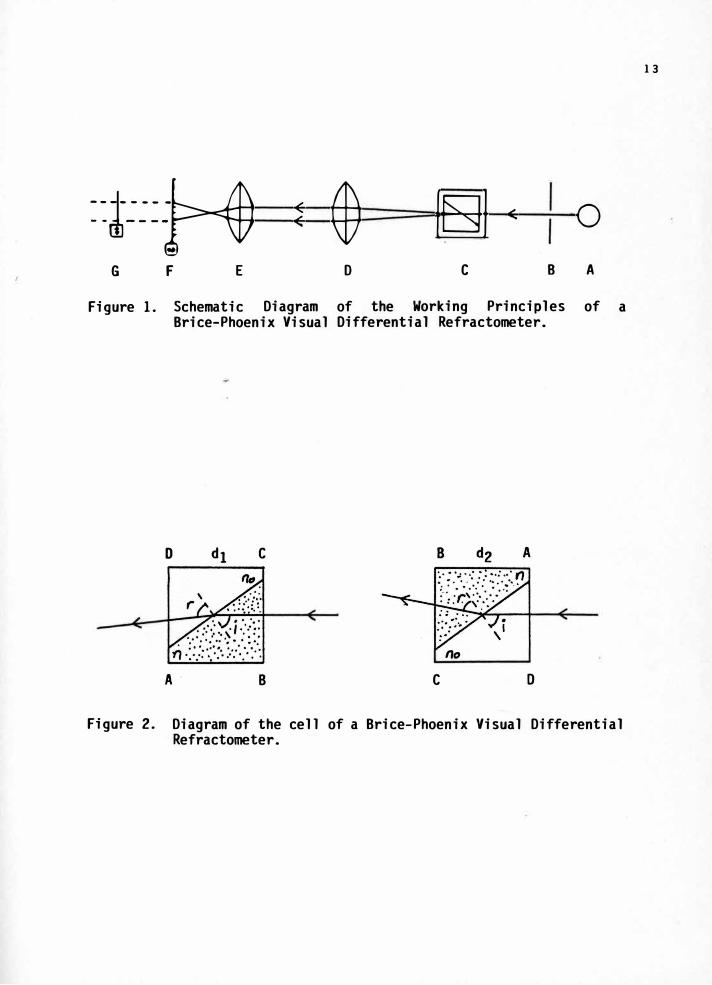
Figure 1 shows the working principle of a Brice-Phoenix visual
differential refractometer. The monochromatic light beam coming out
of the light source (A), passes through an adjustable slit (B), and
goes through a sinter-fused optical glass cell (C) which contains
the solution and solvent that are separated_ from each other by a
diagonal glass partition. The glass cell is clamped so that the
polished faces are perpendicular to the optic axis. The cell holder
can be rotated about a vertical axis through 180°. As seen in
Figure 2 when the light beam enters from the solution side and exits
from the solvent side, the reading is d1, and when the light beam
enters from the solvent side and exits from the solution side, the
reading is d2, The light beam that leaves the cell, which is an
image of the slit, is projected by a projector lens (D) onto the
focal plane (F) of the objective of a microscope (E). The slit
image can be focused by moving the microscope objective on the
longitudinal axis. Values of d1 and d2 are obtained, when the
movable cross-hairs in (G) are exactly in the center of the image of
the slit, or the focal plane. This is done by the aid of a_ drum
that moves the cross-hairs and is divided to 0.01mm.
12
--1---�- - ----
..
G F E
Figure 1. Schematic
:
Diagram Brice-Phoenix Visual
D C
A· B
© IEJI ( 0
D C B A
of the Working Principles of a Differential Refractometer.
no
C D
Figure 2. Diagram of the cell of a Brice-Phoenix Visual Differential Refractometer.
13

The refractive index difference is given by the following
equation28:
An = k •Ad (1.16)
Where An is the refractive index difference between a solution
and its solvent, k is the calibration constant for the selected
wavelength, and Ad is the difference reading on the instrument
between solution and solvent. The reading of total displacement,
Ad, corrected for the solvent zero reading, is calculated as
follows:
where (d2-d1) is the reading of the solution,
and (d2'-d1') is the zero reading of the solvent (Fig. 2).
According to Bushuk and Benoit26, the specific refractive
increment for binary copolymers expressed as a colligative property
takes the form:
where
V • x1v1 + (l-X1) V2 (1.17)
Vl = (dn/dc>1
V2 = (dn/dc)2
V • (dn/dc>1.2
cl , the weight fraction of component 1, c1 + c2 where c is g/mL.
Thus, according to equation (1.17), if the specific refractive
increment for the two homopolymers is known in a given solvent, the
weight fraction of both components can be calculated by determining
V for the copolymer. The mole fraction can be calculated from the
weight fraction through the following relationship:
14
1
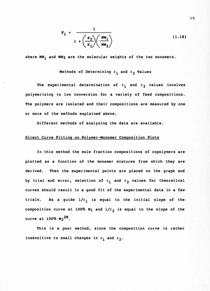
l ·G�(::)(1.18)
where MW1 and MW2 are the molecular weights of the two monomers.
Methods of Determining r1 and r2 Values
The experimental determination of r1 and r2 values involves
polymerizing to low conversion for a variety of feed compositions.
The polymers are isolated and their compositions are measured by one
or more of the meEhods explained above.
Different methods of analyzing the data are available.
Direct Curve Fitting on Polymer-Monomer Composition Plots
In this method the mole fraction compositions of copolymers are
plotted as a function of the monomer mixtures from which they are
derived. Then the experimental points are placed on the graph and
by trial and error, selection of r1 and r2 values for theoretical
curves should result in a good fit of the experimental data in a few
trials. As• a guide l/r1 is equal to the initial slope of the
composition curve at 100% M1 and l/r2 is equal to the slope of the
curve at 100% M229.
This is a poor method, since the composition curve is rather
insensitive to small changes in r1 and r2.
15

Intersecting Slopes Method
In this method r1 is allowed to take on selected values in the
composition equation (1.13) for a single copolymer composition
result and the corresponding r2 values are calculated by an equation
derived from equation 1.13 shown below.
r2• CJ 2 (
1
:•) r1 • C,)e-:•)
where f =- F =
M1 and M2 are concentrations of monomer 1 and 2 in monomer mixture
and m1 and m2 concentrations of monomer 1 and 2 in copolymer.
Calculated values of r2 are plotted as a function of r1. Each
experiment with a given feed composition gives a straight line, the
region of intersection of several of these allows the evaluation of
r1 and r2. Because of the experimental errors, the lines generally
do not intersect in a single point; the region within which the
intersections occur gives some information about the precision of
the experimental results.
Fineman and Ross Method
The copolymerization equation (1.13) is rearranged to the
form30.
g(G-1) g2
G
=r1G
-r2
(1. 19)
where M1
G ml g =
M2 m2
16

M1 and M2 are concentration of monomer 1 and 2 in the monomer
mixture and m1 and m2
concentration of monomer 1 and 2 in the
copolymer.
A plot of g(G-1)/G as ordinate and g2/G as abscissa will result
in a straight line with a slope of r1 and an intercept of -r2•
Equation 1.13 can also be rearranged as follows, in this case
G-1_§_ = -r
2 + rl ( 1. 20) g 92
slope is -r2
and the intercept is r1,
The data cal! be plotted and a least squares method can be
applied to determine the slope and intercept.
Kelen and Tudos Method
Kelen and Tudos31 developed the linear equations 1. 21 and 1.22.
(1.21)
and/or Tl r
2 (1- t ) = rl t -(J
(1.22)
g(G-1)/G g2/G where 11 =
CJ+ g2/G , t =
+ g2/G(J
G and g have the same meanings as used for Fineman-Ross Method.
If X=g2/G and Xm stands for the lowest and XM for the highest values
of the X values calculated from the series of measurements, then the
choice of CJ = VXm•XM will afford optimum distribution of the data.
The t cannot take any positive value, only those in the
interval (0, 1). Thus plotting the Tl values calculated from the
experimental data as a function oft, one should obtain a straight
17

line, which extrapolated to t=O and t=l gives -r2/a and r1 (both as
intercept).
Quantitative Treatment of Composition Drift
A general formula for obtaining the copolymer composition for
any conversion was developed by Skeist32 •
Be considered a mixture of two monomers, of mole fractions f1
and f2, respectively. If the total amount of both monomers is M
moles, then there are f1M moles of the monomer 1 in the original
monomer mixture. · If dM moles of monomer polymerize, the number of
moles of monomer 1 in the polymer is F1dM, where F1 is mole fraction
of monomer 1 in the copolymer. At the same time, the number of
moles of monomer 1 in the monomer mixture has been reduced to
The material balance of monomer 1 gives
f1M-(M-dM) (f1-df1) • F1dM, and by neglecting the product of two
differentials Mdf1 + f1dM = F1dM, leading to dM/M = df1/(F1-f1). By
integrating both sides, he obtained
= ff
,flO
ln M 1
Mo
(1. 23)
where M = M1 + M2 and Mo = M1° + M2°
. M is the total number of
moles in monomer feed at a given time t of the copolymerization and
Mo is the total number of moles in monomer feed at time zero. For
given values of the reactivity ratios, graphical or numerical
methods can be used to calculate the expected change in the monomer
18
mixture and copolymer composition corresponding to the mole
conversion, l-M/M0•
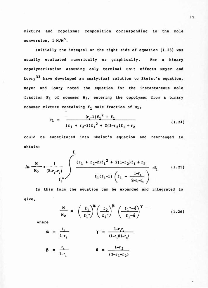
Initially the integral on the right side of equation (1.23) was
usually evaluated numerically or graphically. For a binary
copolymerization assuming only terminal unit effects Meyer and
Lowry33 have developed an analytical solution to Skeist's equation.
Meyer and Lowry noted the equation for the instantaneous mole
fraction F1 of monomer M1, entering the copolymer from a binary
monomer mixture containing f1 mole fraction of M1,
( 1. 24)
could be substituted into Skeist's equation and rearranged to
obtain:
M 1 ln--=---
Mo (2-r1-r2)
ro
1
(1. 25)
In this form the equation can be expanded and integrated to
give.I
M
( ff11J (
ff22.)
8
( f1•-a
J Y
= (1.26) Mo f1-6
where
(J = ...:l_ y =
1-r{ll
1-r 2 (1-r 1)(1-r 2)
8 = ...:L_ 6 =
l-r21-r
1 (2-r1-r2)
19

k22 r ---2- k21
with the condition r1 :;t:l and r2:;t:l.
Kruse34 rearranged the form of the existing integrated
copolymerization equation to a form that enables one to easily do
the calculation of average copolymer composition versus extent of
polymerization.
The copolymerization equation in its usual form is1:
dM1 M1 -- = -- • -----( 1. 27)
where M1 and M2 are the molar concentrations of the two monomers and
r1 and r2 are the reactivity ratios. Equation 1.27 has been
integrated by Mayo and Lewis3 from initial values of M1° and M2
° to
values of M1 and M2 at any extent monomer conversion (p) to yield:
M2 _:1... M2° M1
ln = ln M2
0 l-r2 M1 ° M2
l-r1r
2 ( r 1-1 )(M1/M2 )-r 2 + 1ln
( 1. 28)
(l-r1)(1-r2) (r1-l)(M10 /M2
0 >-r2 + 1
Rearranging eq. (1.28) leads to eq. (1.29):
Since the calculation of F1 as a function of p is difficult
with the equation in this form, Kruse redefined the variables in
eq. ( 1. 29).
20

His definitions are listed below:
f1 ° = the initial mole fraction of component one in themonomers
f1 = final mole fraction of component one in the monomers
f 0
2 = 1-flo
M0
= the total initial number of moles of both monomers
{ l-p)M0 = the number of moles remaining after an extent of reaction p. With these definitions:
M1 "" f1{1-p)M0
M2 = f2{1-p)M0
By subs ti tu ting these quantities in eq. { 1. 29) and rearranging
them, one obtains:
=
(
t-f
-'1'2
( t f -<1<2
The extent of reaction p is
[ ] l
-<1<2{l-r2>f2
0 -{l-r1)f10
{l-r2)f2-{l-r1)f1 {1.30)
now expressed as a function of, the
initial and final monomer mole fractions. This eq. {1.30) is
equivalent to Meyer and Lawry's eq. {1.26).
From a component balance on the number of moles one can
calculate F1, the average polymer composition.
(1. 31)
Solving for F1,
(1. 32)
21

For a given f1 °, r1 and r2, the calculation procedure simply
involves assuming a value of f1 and calculating a value of p with
eq. (1.30) and then a corresponding value of F1 by eq. (1.32). By
assuming various values of f1, one can determine the complete curve
of F1 versus p.
Goals of Current Research
Monomer reactivity ratios, r1 and r2' of copolymers can be
determined by var�ous methods as seen in the above discussion. The
goal of this research is to apply the methods to the very carefully
conducted experimental copolymer composition data to evaluate the
best r1 and r2 values and to see how well these calculation methods
compare to each other.
In the literature there is a significant deviation in r1 and r2
values reported for the poly(styrene-co-methyl methacrylate) system.
The r1 and r2 values seen below were obtained at 60.0°C by various
workers using styrene as monomer one and methyl methacrylate as
monomer two.
rl r2 References
0.52 ± 0.026 0.46 ± 0.026 35
0,50 ± 0.02 0.50 ± 0.02 36
0,48 0.46 37
0.44 ± 0.08 0.50 ± 0.04 38
0.54 ± 0.04 0.42 ± 0.1 38
0.536 ± 0.02 0.50 ± 0.06 39
22
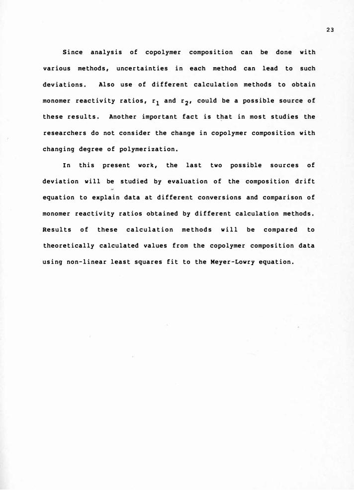
Since analysis of copolymer composition can be done with
various methods, uncertainties in each method can lead to such
deviations. Also use of different calculation methods to obtain
monomer reactivity ratios, r1 and r2, could be a possible source of
these results. Another important fact is that in most studies the
researchers do not consider the change in copolymer composition with
changing degree of polymerization.
In this present work, the last two possible sources of
deviation will be studied by evaluation of the composition drift
equation to explain data at different conversions and comparison of
monomer reactivity ratios obtained by different calculation methods.
Results of these calculation methods will be compared to
theoretically calculated values from the copolymer composition data
using non-linear least squares fit to the Meyer-Lowry equation.
23
CHAPTER II
EXPERIMENTAL
Preparation of Low Conversion Styrene-Methyl Methacrylate Copolymers
Styrene and methyl methacrylate (both reagent grade, Fisher
Scientific Company) were purified by distillation under low pressure
immediately before use. Calcium metal was added before distil-
lation. The center fraction (about 80%) of styrene was collected
at 60°C and 45 torr. The center fraction (about 80%) of methyl
methacrylate was collected at 35 °C and 39 torr. The purity of the
monomers was checked by gas chromatography and no impurities were
found.
Polymerizations were done in sealed pyrex tubes, in a constant
temperature bath. Each monomer was directly weighed into a narrow
necked pyrex tube. After thorough mixing of the monomers, dibenzoyl
peroxide (Aldrich Chemical Company, Inc.) 0.1% by mass of mixture
was added as an initiator, the tubes were swept with nitrogen and
were sealed under vacuum.
Nine groups of copolymerization mixtures were prepared. Each
group contained eleven tubes, having 100, 90, 80, 70, 60, SO, 40,
30, 20, 10, and O mol % styrene. The total mass of the monomer
mixture in each tube was approximately lOg.
The first group of each of the above concentrations of monomers
was polymerized for one hour in a constant temperature water bath at
60.0 ± 0,1°C. The second group was polymerizied for two hours, the

third group for three, the fourth group for four, the fifth group
for five, the sixth group for six, the seventh group for seven, the
eighth group for eight, the ninth group for nine hours. At the end
of the polymerization time, the eleven tubes belonging to each group
were removed from the water bath and quickly cooled in dry ice.
Purification of Copolymers
Each copolymer was precipitated in 1000 to 1200 mL of methanol
(Certified, Fisher' Scientific Company) and the polymer was redis
solved in 30 to 50 mL of methyl ethyl ketone (Certified, Fisher
Scientific Company) and reprecipitated in 1200 to 1500 mL of
methanol. The polymer then was filtered through quantitative filter
paper (Whatman 42 ashless) with the aid of vacuum using a Buchner
funnel and air dried.
Each copolymer sample was then dissolved in eight to ten times
its mass of benzene (Analytical reagent, Mallinckrodt) in a flask
and the solution was frozen in dry ice. The flask was then
transferred to an ice bath and held at 0°C at 1-2 torr pressure to
sublime the benzene from the polymer. About 40 to 45 hours were
required for sublimation of most of the benzene. This frozen
benzene technique40 assures complete removal of solvent and
unpolymerized monomers.
25

Removal of the remaining traces of solvents was completed by
drying in a vacuum oven for 40 to 45 hours at 45 °C and about
8-10 torr pressure. The conversion was determined by weighing.
The percent conversion values are given in Appendix e, Table I.
Determination of Copolymer Composition
Method of Obtaining Refractive Index Increments
The refractive index increments were determined using a Brice
Phoenix differential refractometer, model BP-2000-V. This differen
tial refractometer allows determination of the difference in
refractive indices between a dilute solution and its solvent with a
sensitivity of about ± 0.000003.
The temperature can be controlled easily, because both the
solvent and solution are examined simultaneously in a single cell,
separated from each other by a thin diagonal glass partition. The
ambient temperature need not be closely controlled since the
temperature coefficient of the difference in refractive index
between a solution and its solvent is much smaller than the
temperature coefficient for the refractive index of solution or
solvent alone. However, the solution and solvent in the differen
tial cell should have the same temperature to within 0.01°C.
The instrument was calibrated by using solutions having known
refractive index differences between solution and solvent. In the
present work, distilled water solutions of potassium chloride at
different concentrations were used as reference solutions. In
26
preparing the test solutions, potassium chloride (reagent grade,
Fisher Scientific Company), was dried at approximately 90°C for
3-4 hours. The distilled water for all calibration solutions was
taken from the same batch, because the instrument is sensitive
enough to detect differences between water from different batches.
Some of the distilled water used in preparing the solutions was
retained for use as the reference solvent.
In the present work, the mercury green line (546nm) was used
throughout and the instrument was calibrated to give the
relationship;
An = 0.9144 x 10⁻⁴ Ad.
In preparation of solutions of copolymer, methyl ethyl ketone
(Fisher Scientific Company, A.C.S. Certified) and ethyl acetate
(Fisher Scientific Company, A.C.S. Certified) were used as solvents.
Samples of 0.0100g of each copolymer were dissolved in 10.0000g of
solvent. In calculation of concentrations as g/mL, density vs.
temperature graphs of each solvent were used41 • For each sample the
dn/dc value was calculated using the An value and the concentration.
From these dn/dc values, the values of the mass fraction and the
mole fraction of styrene in copolymer were calculated by using eq.
( l. 16 and l. l 7) .
These values can be seen in Appendix B, Table II.
27
UV Absorption Spectra of Copolymers
Samples of the lowest conversion copolymers of each monomer feed
composition were prepared by weighing out 10.0mg of polymer,
dissolving it in chloroform (UV cut off 244nm, from Burdick &
Jackson Laboratories, Inc.) and diluting to a concentration of
l.Omg/mL. The absorbance of each sample was determined at 269nm in
a Beckman DU-6 Spectrophotometer.
Also solutions of these polymers were prepared in such a way
that each sample nad 1mg of styrene units per mt. The UV absorption
spectra were obtained by a Hewlett Packard 8451 A Diode Array
Spectrophotometer over the wavelength range of 240nm to 300nm.
28
CHAPTER III
RESULTS AND DISCUSSION
Results of Conversion Studies
The purpose of this study is to compare the calculation methods
commonly used to obtain monomer reactivity ratios in free-radical
copolymerization studies. Conversion versus time data can be seen
in Appendix A, Table I and Appendix e, Table I.
At low conversions, which is the point of interest in this
present work, an approximately proportional relationship between
time and conversion to polymer was obtained as expected. Generally
in first order kinetics the logarithm of conversion is plotted
against time. In this study percent conversion versus time was
plotted, as this way is used more frequently in polymer literature.
The following formulas42 were used for estimating the
proportionality constant from experimental values of x and y for the
relationship y=mx.
m=IxiYi / Ixi2
On these,
m is the best value of the proportionality constant, slope.
Xi is the time in hours, and
Yi is the percent conversion.
Also, ay2= -
1- (Iy - mix) 2
(n-1)
( 3 .1)
( 3. 2)
where, ay is the estimated standard deviation of the y-residuals,
29

n is the number of experimental points,
( 3. 3)
where, am is the standard error of estimate of the slope.
For each monomer composition, the rate obtained by the slope of
the percent conversion versus time plots and. the standard error of
the estimate of the slope, were calculated.
A plot of the rate of polymerization versus mole percent of
styrene in the monomer mixture can be seen in Figure 3. The
horizontal lines above and below the data points represent the
standard error of· estimate of the proportionality constants. The
reverse J shape of the curve that was obtained is similar to the
shape of similar plots given in the literature43 by previous
investigators.
As this subject is not the central point of interest in this
study no further investigation has been done in this area. However,
as the data were consistent with expectations and was available, it
has been included to assist further researchers.
Copolymer Composition Studies With Refractive
Index Increment Measurements
In this study the weight fraction and mole fraction of styrene
in the copolymer is determined by refractive index increment
measurements. The calculation method and formulas used are
explained in the Introduction Chapter and their results can be seen
in Appendix A, Table II.
30

31
2.5
2.0 -
0
0
1.5 -
0
D C
• 1.0
0 20 40 60 80 100
f.1ole Percent Styrene
Figure 3. Rate of Copolymerization of Styrene and Methyl Methacrylate, in mole percent per hour, at 60.0 ± 0.1°C. Horizontal bars represent standard error of estimate.

The average deviation and estimated standard deviation values
can be calculated by,
and,
Average deviation =
Standard deviation = Average of average deviation x y,./2
� Average of average deviation x 1.25
(3.4)
( 3. 5)
where Fis the mole fraction of styrene in copolymer in methyl ethyl
ketone or ethyl acetate. These values can be seen below where f is
the mole fraction �f styrene in monomer mixture.
I Estimated Standard Deviation
~ 0.1 0.001171
~ o. 2 0.000341
~ o. 3 0.000446
~ 0.4 0.000595
~ 0.5 0.000462
~ 0.6 0.001710
~ o. 7 0.001094
~ 0.8 0.000162
~ 0.9 0.000699
Evaluation of Methods of Estimating Reactivity
Ratios from Experimental Data
Maximum Likelihood Method
The most probable values of parameters in a mathematical model
based on the experimental data obtained were found by using a least
squares computation.
32

The outcome of this computation will be valid if the model is
correct and if there are no systematic errors in the data and no
random errors in the independent values of f and conversion.
The best fit is found by computing the expected value of F
corresponding to each experimental value of f and the observed
conversion. The difference between F and F is the "residual" of the
data point (i.e., it is the amount of apparent error remaining after
computing the expected value).
This computation is done for all data points for a given assumed
set of values of ·parameters, r1 and r2. All the residuals for a
particular set of r1 and r2 are squared and summed together to give
the sum of squares of residuals, "SSR."
It can be shown by application of the probability theory that
the best possible estimate of parameters consistent with the data
set will be that set of values of r1 and r2 that gives a lower value
of SSR than does any other set of parameter values. This is
generally true whenever the random errors in the dependent variable
(F) are symmetrically distributed, e.g. normally distributed.
If SSR is plotted as a function of r1
and r2
on a three
dimensional Cartesian plot, the values form a surface that is
approximately an elliptical paraboloid. The lowest value of SSR
(the "least-squares" value) is at the vertex, or bottom tip of the
paraboloid. This 'is true both in a linear equation such as y=mx+b
and in more complex equations. The linear case equations can be
solved algebraically to calculate the best values of m and b. When
33

the equations cannot be solved for more complicated cases, such as
the present one, numerical calculations must be used to estimate the
location of the minimum point on the SSR surface.
Various methods have been proposed and used. In this case a
simple three by three grid search procedure is used, with the final
grid spacing set at a value to yield five significant figures. By
the nature of a gr id search, the value obtained is not necessarily
within the five-figure precision of the true minimum of the surface,
but it probably is within four-figure precision, and almost
certainly within three-figure precision. The value obtained in this
way is used as the basis of comparison of other methods.
In this method the formulas of the Lowry and Meyer equation
(1.26), together with a rearrangement of the Kruse equation (1.32),
were used to compute the maximum likelihood values of r1 and r2•
The actual computations of SSR values were done with the aid of a
computer program written by Dr. G. G. Lowry.
First, a particular set of values of r1 and r2 is chosen
consisting of three values for each parameter. The initial choice
is made with central values at one significant figure precision for
both r1 and r2. Then additional values of each parameter are chosen
that are both larger and smaller than the central values. The
amount of difference is l in the same decimal place location as the
precision of the central values. Thus, choosing the central value
of 0.5 for both r1 and r2 yields a 3 x 3 grid as follows:
34

0.4
r1
0.5
0.6
0.4 0.6
Then for each of the nine points on this grid, the following
procedure was used. The computer calculates the monomer composition
at the experimentally determined conversion with the initial monomer
composition and the assumed r1 and r2 values. For this calculation
numerical values are given to solve the Meyer-Lowry equation. Then
the average copolymer composition corresponding to these values is
calculated. For this the material balance equation developed by
Kruse is used. This copolymer composition is called the estimated
copolymer composition. The residual is obtained by subtracting the
estimated copolymer composition from the observed copolymer
composition. Each residual is squared and the sum of these squared
residual, SSR, is calculated. This calculation is reported for each
of the nine assumed sets of r1 and r2 values.
Then the grid search method is used to obtain the best r1 and r2
values. In this method the calculation is started with the assumed
r1 and r2 values that differ by an increment of 0.1 units. This
estimation is based on literature values of similar studies. The
objective is to obtain the smallest value for SSR in the middle box
of this grid. If the smallest of the nine SSR values obtained thus
is not in the middle square of the grid the r1 and r2 values that
gave that value is placed in the middle of a new grid with the same
35

spacing of r1 and r2. The calculation is continued until the
smallest SSR value is in the center position.
Then the grid size is "shrunk" to one-tenth the initial spacing.
The central values of r1 and r2 on the new, smaller grid are those
that gave the smallest value of SSR with the _initial grid size. The
additional values of r1 and r2 are then greater and smaller than the
central values by 0.01. Thus the original 3 x 3 grid has a spacing
of 0.1, and the new, smaller grid has a spacing of 0.01. The
computations of SSR are continued with this grid spacing until the
lowest value of SSR corresponds to the central r1 and r2 values for
a grid. The process is repeated with grid spacings of 0.001, then
0,0001, and finally 0.00001.
The r1 and r2 values at five significant figures that
corresponds to this smallest SSR are then accepted as the best r1
and r2 values that will be used as a base for comparison of
different methods of finding r1 and r2. The other methods which are
discussed next were used to estimate r1 and r2 to a precision of
five significant figures for comparison. The best fit (maximum
likelihood) values of reactivity ratios, r1 and r2, are found to be
0.49520 and 0.46669 respectively.
This method however is tedious and lengthy even with a �om�uter.
Therefore, it is desirable to find a simpler method that will give
estimates of r1 and r2 as close as possible to these values. A
contour plot (Fig. 4) serves as one criterion of evaluating how good
the other fitting methods are.
36

0.52
0.47
0.42
0.45 0.50 0.55
Figure 4. Contours Representing Surface of Residuals-Squared ·for Non-linear least Squares Fitting of Weighted Styrene-r1ethyl Methacrylate Copolymer Data. Points Represent Different f-1ethods of Evaluation, f1aximum Likelihood (A), Non-linear Least Squares (o), Intersection (□), Kelen-Tudos Method(◊), Fineman-Ross (v).
37

To draw the contour plot, the values are computed at SSR at many
coordinates of r1 and r2 and are interpolated to find coordinates of
points with same values of SSR.
through these calculated points.
Then contour lines are plotted
The value of SSR at the minimum
according to this method was 0.003772.
Methods Using Extrapolated Zero-Conversion Data
As seen in Figure 5 the F versus conversion lines show no
significant curvature over the range of conversions studied. Thus
for a simpler computational method, all F values for each f value
were fitted by ordinary linear least squares to obtain the intercept
with its uncertainty. This value corresponds to zero-conversion
extrapolated values, that is, to the instantaneous copolymer
composition to which the Mayo equation applies. Then for each
method a single data point for each monomer composition is used.
The uncertainty of F is available from the ordinary linear least
squares fit. In the calculation of each average value of f, the
values for a set of data are very close to each other but · not
identical because of instrumental and equipment limitations. In
calculations the average f values were used and their uncertainties
were included in the method of intersections.
Whenever "weighted" data are referred to in the following
sections, the weighting factors are the reciprocals of the squares
of the uncertainties of individual values. Sometimes the weighting
38
0.84
0.82
0.72
0.70
0.64
0.62
0. 570 0
0.55
0.50 0
Fl 0.48
0.45
0.43
0.36
0.34
0.28
0.26
0.18 0 0 0 0 0 0 0
0.16
0 2 4 6 8 10 12 14 16 18
Percent Mole Conversion
Figure 5. Mole Fraction of Styrene in Copolymer Mixture (F1) Versus Percent Mole Conversion. Circles Represent Actual Data Points, Solid Lines are Calculated Results Assuming r1=0.495 and r
2=0.467.
39
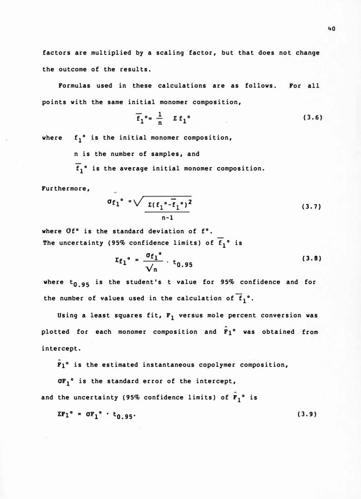
factors are multiplied by a scaling factor, but that does not change
the outcome of the results.
Formulas used in these calculations are as follows.
points with the same initial monomer composition,
where f1° is the initial monomer composition,
n is the number of samples, and
f1° is the average initial monomer composition.
Furthermore,
a f1 o = V E < fl o -f
l o > 2
n-1
where Of0 is the standard deviation of f0•
The uncertainty (95% confidence limits) of f1° is
For all
( 3. 6)
(3.7)
(3.8)
where t0. 95 is the student's t value for 95% confidence and for
the number of values used in the calculation of f1°.
Using a least squares fit, F1 versus mole percent conversion was
plotted for each monomer composition and F1° was obtained. from
intercept.
F1° is the estimated instantaneous copolymer composition,
aF1
° is the standard error of the intercept,
and the uncertainty (95% confidence limits) of F1° is
( 3. 9)
40

Nonlinear Least Squares
Using the values of f1° and F1
° , obtained above, a 3 X 3 grid
search yielded the data listed below.
Table 1
Copolymer Composition Data Using Weighted
Nonlinear Least Squares
f F1 (observed) Weight F1 (calculated) residual
0.10018600 0.17596100 0.02428480 0.16857200 -0.00738952
0,20009900 0.28244800 0.11501100 0.28131800 -0.00113018
0.30002100 0.36719200 0.19784700 0,36687300 -0.00031942
0.40001300 0.43987100 0.05462130 0.43868200 -0.00118898
0.49999900 0. 4.9993900 0 .14987800 0.50459400 0.00465441
0.60003000 0.56365300 0.02182560 0.57054700 0.00689381
0.69998800 0.64100000 0.02936130 0.64228000 0.00128060
0,79999100 0.72996400 0.30681000 0. 72743600 -0.00252816
0.89999100 0.83524100 0.10036100 0,83838900 0.00314707
Intersection Method
In this method as explained in the Introduction Chapter locating
the best values of r1 and r2 from the "probable area" confined by
different straight lines on the r1 versus r2 plot is done using the
subjective judgment of the observer. This judgment introduces a
source of an undetermined amount of error. To overcome this
difficulty, in this present work the weighted average values of r1
and r2 computed from all possible intersections of pairs of lines is
used. The calculation of the uncertainties of these weighted
averages does provide an objective measure of the degree of
precision in the experimental data. Figure 6 shows the r1 versus r2
plots in which the nine lines representing the nine values of
! 1° and F1
° are numbered.
41

0.8
0.6
0.4
0.2
0 0.2 0.4 0.6 0.8
Figure 6. Illustration of the Application of the Intersection Method to the Data of Table 1. The Values on the Figure are Approximate Monomer Compositions, Actual Compositions are Given in Table 1.
42

To estimate the uncertainties in r1 and r2 values of the various
points of intersection on this graph, it was first necessary to
obtain the uncertainties of
described earlier.
the f 0 l and F1°
data points as
Each of the lines in Figure 6 is plotted using the following equa-
tion, with zero-concentration extrapolated values, F1° and f1 ° of
F and corresponding f inserted for each line. The r1 and r2 values
for each intersection point were calculated using the following
formulas.
where f1
is the mole fraction of styrene in monomer mixture, and
F1 is the mole fraction of styrene in copolymer.
This straight line equation can be represented by the simpler form
r2
• ar1+b.
The uncertainties of a and b for each line were calculated using the
usual form for computing propagated error in derived quantities. In
this case,
e. { ( :f•. )'e2 f1 •
Eb -[ (:f
�) 2E2 £1•
For the intersection of each pair of lines i and j,
bj-bi
ai-aj and
aibj - ajbi
ai - aj
and the uncertainties of these values are given by
43
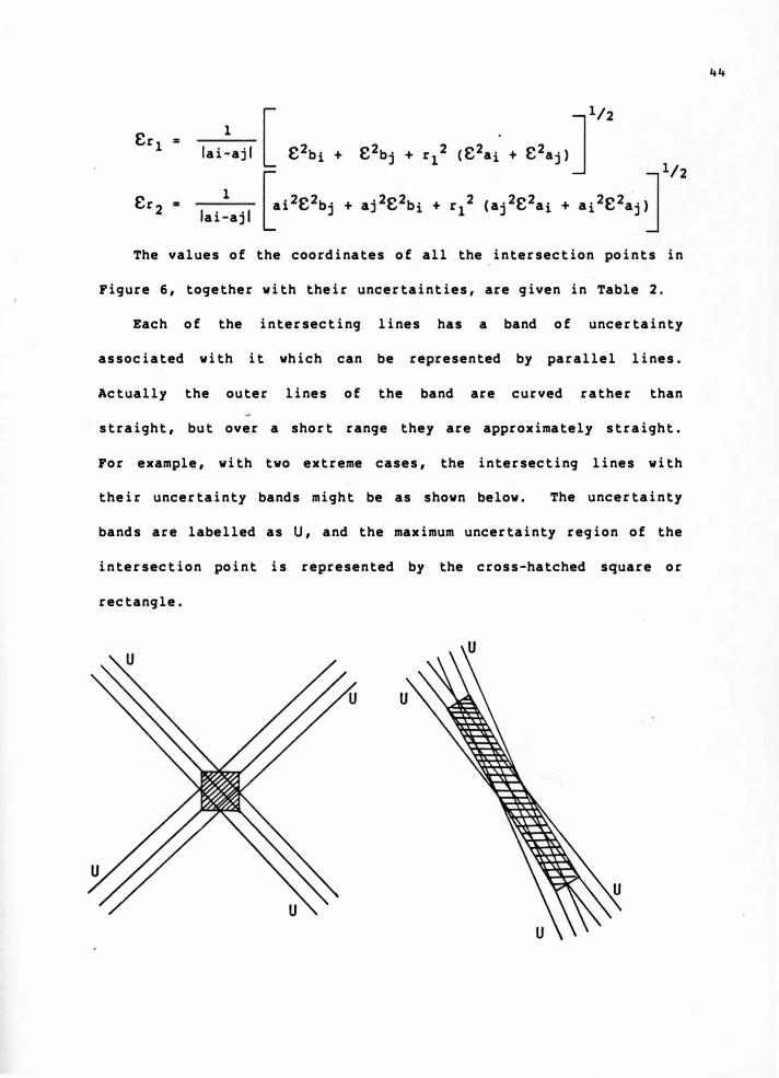
Er11
lai-aj I
Er21
lai-ajl
The values of the coordinates of all the intersection points in
Figure 6, together with their uncertainties, are given in Table 2.
Each of the intersecting lines has a band of uncertainty
associated with it which can be represented by parallel lines.
Actually the outer lines of the band are curved rather than
straight, but ove_r a short range they are approximately straight.
For example, with two extreme cases, the intersecting lines with
their uncertainty bands might be as shown below. The uncertainty
bands are labelled as U, and the maximum uncertainty region of the
intersection point is represented by the cross-hatched square or
rectangle.
44

45
Table 2
Monomer Reactivity Ratios and Uncertainties at Each Intersection Point
Intersecting lines rl Er1 r2 Er1
1-2 0.2475 0.0491 0.4244 0.0073
1-3 0.3869 0.0186 0.4325 0.0056
1-4 0.4485 0.0108 0.4361 0.0051
1-5 0.4350 0.0054 0.4353 0.0049
1-6 0.4447 0,0052 0.4359 0.0048
1-7 0.4803 0.0036 0.4380 0.0047
1-8 0.5000 0.0013 0.4391 0.0046
1-9 0.4796 0.0022 0.4379 0.0046
2-3 0.4759 o. 014 7 0.4607 0.0039
2-4 0.4982 0.0087 0.4643 0.0028
2-5 0.4574 0.0034 0.4578 0.0022
2-6 0.4573 0.0049 0.4578 0.0021
2-7 0.4884 0.0035 0.4627 0.0020
2-8 0.5044 0.0011 0.4652 0.0019
2-9 0.4811 0.0022 0.4615 0. 0019
3-4 0.5123 0.0135 0. 4722 0.0051
3-5 0.4532 0.0039 0.4535 0.0023
3-6 0.4552 0.0054 0.4542 0,0030
3-7 0.4892 0.0036 0.4649 0.0020
3-8 0.5052 0.0011 0.4700 0.0018
3-9 0.4812 0.0023 0.4624 0.0016
4-5 o. 4192 0.0086 0. 4195 0.0075
4-6 0.4431 0.0069 0.4331 0.0057
4-7 0.4868 0.0041 0.4578 0.0043
4-8 0.5049 0.0012 0.4681 0.0034
4-9 0.4807 0.0023 0.4543 0.0034

Table 2 -- Continued
Intersecting lines rl Er1 r2 Er1
5-6 0.4570 0.0017 0.4574 0.00115
5-7 0.5012 0.0050 0.5015 0.0059
5-8 0.5125 0.0013 0.5128 0.0030
5-9 0.4824 0.0024 0.4828 0.0034
6-7 0.5262 0.0100 0.5778 0.0231
6-8 0.5223 0.0024 0.5711 0.0120
6-9 0.4838 0.0026 0.5039 0.0097
7-8 0.5206 0.0042 0.5607 0.0221
7-9 0.4795 0.0028 0.4354 0.0020
8-9 0.4677 0.0035 0.2480 0.0219
Thus in these two cases in which all the lines have the same
width of uncertainty band, there is an extremely large difference in
the size and shape of the uncertainty region of intersection.
Any time the two lines are not at right angles to each other,
the uncertainty region is a rectangle (or perhaps an ellipse) whose
long axis coincides with a line that bisects the smaller angle of
the intersection. The length of the long axis of the region in.the
example is much greater than that of the short axis.
Then the relative uncertainties of the r1 and r2 values depend
not only on the angle at which the lines intersect, but also on the
angle the line of bisection make with the r1, r2 axes.
The following figures illustrate this concept where the
uncertainties on each axis are shadowed. It is seen that the
relative uncertainties of r1 and r2 of intersection are very
46

different for these three cases involving identical size and shape
of the uncertainty regions of intersection.
r 2
It can be see-n from Table 2 that r1 and r2 values vary from
0.2475 to 0.5262 and 0.2480 to 0.5778 respectively. The procedure
commonly used in the past has been to decide from the visual
appearance of a graph such as Figure 6 the most likely set of values
and their uncertainties for r1 and r2. However, by calculating the
results in Table 2 it is possible to obtain the final results in a
more objective way. Thus the weighted average of
r1 and r2 values (r1 and r2) are found from the following formulas,
I (e::, ) I ('2
)Er22
i,j i' j
,. r 1 and ,. r 2
I (e:,, ) 2: (e ,',, ) i,j i,j
The uncertainty in r1 and r2 values are found using the following
equations for the case of r1, and similar equations for r2.
1
47

where, Or1 is the standard error
n=K � 1
Er12
and Er1• . to.9s
where, Er1 is the uncertainty of error of rl
n is the number of intersection points.
By applying the above equations to the values in Table 2, the
weighted average values of r1 and r2
and absolute error in 95%
confidence limits were found to be 0.49581±0.0059 2 and
0.46037±0.00579, respectively.
Although r values are estimated to the precision of three
significant figures they are stated to five significant figures for
comparison between methods.
Fineman and Ross Method
As is illustrated in the Introduction Chapter, in this method
the copolymerization equation (1.13) is rearranged to the form of
where 9 =
..L 9 2
( G-1) = r 1 - r2 ( 1. 19)
G G
G ,.
A plot of g/G (G-1) as the ordinate and 9 2/G as the abcissa is a
straight line whose slope is r1 and whose intercept is -r2. The
uneven spacing of the data points can clearly be seen in Figure 7a
and 7b. Results of the least squares calculations using equation
1. 19 are
48

-
..... I
c.D -
7
5
1
-1 L..--11,---'-�-__...,--4---+--+-----i
0 4 8 12 g2/G
Figure 7a. Fineman-Ross Hethod using Equation 1.19, Styrene as Monomer 1.
-
..... I
c.:, -
7
5
1
-14 8 12 14
g2/G
Figure 7b. Fineman-Ross Method using Equation 1.19, Methyl Nethacrylate as Monomer 1.
49

Monomer l
Styrene
Methyl methacrylate
Equation (l. 13) can also be
G-1= - r2 g
In this case the slope is
0.48286024
0.43888575
rearranged to the
G -2- + rlg
0.45303593
0. 44871682
form of
( l. 20)
-r2 and the intercept is rl. There is
also uneven spacing of the data points on the plot drawn by using
equation 1.20. This can be seen in Figures Ba and Sb. The results
of using equation 1.20 are
Monomer l
Styrene
Methyl methacrylate
0.44872683
0.45303557
0.43888595
0.48285998
According to Fineman and Ross30 , data can be plotted and a least
squares method can be applied to determine the slope and intercept
in both cases. The values of r1 and r2 determined by plotting in
term of equation 1.19 and 1.20 should be in excellent agreement.
It is common practice to give the average values of r1 and r2
for the two cases where monomer one is styrene and monomer one is
methyl methacrylate. For this case these values can be seen below.
Average results from rl r2
Eq. 1.19 0.46578853 0.44596584
Eq. 1.20 0.46579341 0.44596076
Overall 0.46579097 0.44596330
50

0
-2
-4
-6
-8
0 4 8
G/g2 10 12
f;gure Sa. Fineman-Ross Method using Equation 1.20, Styrene as f.1on0111er 1.
0
-2
-4
-6
-8
0 4 8
G/g2
12
f;gure Sb. f;neman-Ross Method usfog Equation 1.20, Methyl Methacryl ate as Honomer 1.
51

Kelen and Tudos Method
Kelen and Tudos introduced a new improved linear graphic method
to calculate r1 and r2 values. They modified the Fineman-Ross
equation (1.19) by adding a parameter, Cl, into the formula of the
straight line. The resulting straight line gives both r1 and r2
values as intercepts. This method has been explained in detail in
the Introduction Chapter.
Experimental results of using this method are shown in Figures
9a and 9b. The results of the least squares computations from these
graphs are
Monomer 1
Styrene
Methyl methacrylate
0.482306608
0.455225229
0.456037653
0.481477279
It is seen that the result of reversing indices or monomers are
much more consistent than in the Fineman-Ross method. Also in these
plots the data points are distributed much more uniformly along the
abcissa.
The two sets of results are not identical because of the
experimental errors in both variables of the linearized equation.
However, the.ir differences are small, and the averages of the two
computations are probably more reliable. These values are,
r1 = 0.481891944 and r2 = 0.455644972, where monomer one is styrene.
Effect of Composition Drift With Conversion
The method of extrapolating to zero conversion prevents a drift
in values. To show this effect Kelen and Tudos non-zero conversion
values were calculated by using about 5% conversions for low
52

0.3
0.1
n -0.1
-0.3
-0.5
0 0.2 0.4 0.6
Figure 9a. Kelen-Tudos Method, Styrene as Monomer 1.
0.1
-0.1n
-0.3
-0.5
0 0.2 0.4 0.6
53
0.8
O.R
Figure 9b. Kelen-Tudos Method, Methyl 11ethacrylate as Monomer 1.
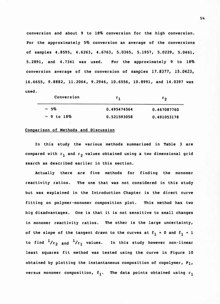
conversion and about 9 to 18% conversion for the high conversion.
For the approximately 5% conversion an average of the conversions
of samples 4.8595, 4.6263, 4.6763, 5.0365, 5.1957, 5.0229, 5.0461,
5.2891, and 4.7341 was used. For the approximately 9 to 18%
conversion average of the conversion of samples 17.8377, 15.0423,
16.6655, 9.8882, 11.2064, 9.2946, 10.6556, 10.8991, and 14.0397 was
used.
Conversion
5%
9 to 18%
0.495474564
0.521593058
Comparison of Methods and Discussion
0.467087760
0.491053178
In this study the various methods summarized in Table 3 are
compared with r1 and r2 values obtained using a two dimensional grid
search as described earlier in this section.
Actually there are five methods for finding the monomer
reactivity ratios. The one that was not considered in this study
but was explained in the Introduction Chapter is the direct curve
fitting on polymer-monomer composition plot. This method has .two
big disadvantages. One is that it is not sensitive to small changes
in monomer reactivity ratios. The other is the large uncertainty,
of the slope of the tangent drawn to the curves at f1 = 0 and f1 = 1
to find 1 /r2 and 1 /r1 values. In this study however non-linear
least squares fit method was tested using the curve in Figure 10
obtained by plotting the instantaneous composition of copolymer, F1,
versus monomer composition, f1• The data points obtained using r1
54

Table 3
Comparison of Methods
Computation Method
Maximum Likelihood
Extrapolated Zero-Conversion:
Non-Linear Least Squares
Intersection
Fineman-Ross
Kelen and Tudos
Non-Zero Conveisions:
(by Kelen-Tudos)
5%
9 to 18%
0.49520
0.49533
0.49581
0.46579
0.48189
0.49547
0.52159
0.46669
0.46810
0.46037
0.44596
0.45564
0.46709
0.49105
SSR
0.003772
0.003787
0.004046
0.008716
0.004795
0.003774
0.007819
and r2 values from the non-linear least squares method has fitted
this curve without any visually noticable deviation.
In this study, the various methods are compared with obtained r1
and r2 values using a two dimensional grid search as described in
Maximum Like.lihood Method. The r1 and r2 values obtained with the
four different methods are shown all together on the graph seen in
Figure 4. This figure was obtained by doing the SSR calculation on
a grid basis and the calculated contour lines of equal SSR values
were plotted, using interpolation between calculated levels of SSR.
The best method is the Non-Linear Least Squares Method that
gives a point almost at the center of the ellipsoid contour.
55

0 0.2 0.4 0.6 0.8 1.0
Figure 10. Instantaneous Composition of Copolymer Fi as a Function of Monomer Composition �1 for the Values of ReactivityRatios, r1 and r
2, 0.49!f and 0.467. Circles Represent
Copolymer Composnion Extrapolated to Zero Conversion, Solid line is Calculated value.
56

However the following conditions must be met for the accuracy of
this method.
l. The mathematical model, a combination. of the Mayo
equation and the Meyer-Lowry equation, is correct.
2. There are no systematic errors in analysis of the
polymers for their composition.
3. There are no systematic errors in the determination
of the conversion of the polymers.
4. There are only random errors in the copolymer
composition.
s. Any systematic errors present are negligibly small.
In the Fineman-Ross and Kelen-Tudos methods the non-linear form
of the Mayo equation is linearized to fit a straight line to the
adjusted data. This linearization reduces the accuracy of the
results calculated by these methods in two ways. First, it distorts
the error structure so that even though all the original data points
may have the same uncertainty, the errors of the adjusted values
that are plotted are not the same. Secondly, this adjustment of
data introduces uncertainty in both abcissa and ordinate data even
though. in the original data there is no uncertainty in abcissa
values. Ordinary least squares calculations are applied to these
methods, but the ordinary least squares method assumes no error in
abcissa and equal uncertainty of all data points. Fur thermo re the
original data are uniformly spaced along the horizontal axis.
57
The Fineman-Ross method distorts the data so that some of the
resulting adjusted values have a greater influence on the slope and
intercept of the line than they should. Therefore, the largest
deviation is seen in the Fineman-Ross method using the equation 1.19
and l. 20. Indeed it can easily be seen that r 1 and r 2 values
obtained by applying the same experimental data to equation 1.19 and
1.20 gives different results. Also, different r1 and r2 values are
obtained in cases where calculations are made using styrene as M1 in
one case and methyl methacrylate as M1 in the other case.
The Kelen-Tu-dos method avoids the problem of unbalanced
weighting of some points. The data points are spread so that they
have nearly equal influence on the slope and intercept of the line.
However, the adjusted data used still introduce uncertainty of
abcissa and ordinate values. Because of this as well as the possi
bility of rounding off errors, exchanging the monomer M1 and M2 will
not give identical r1 and r2 values. It would seem appropriate to
use the average so it would compensate the error. This will not
rigorously justify statistical error but practically compensate it.
In the Intersection method as some intersection points have more
uncertainty those points should be weighted much less heavily than
the others to determine the average value. In calculations if the
uncertainty of each value is weighted according to reciprocal square
of the uncertainty, the intersection method becomes a very accurate
method to calculate r1 and r2 values.
The experimental data in this research have led to another
valuable observation. In Figure 5 for some of the concentrations
58

all the points either are above or below the calculated composition
lines. This effect seen in Figure 11 gives a sinusoidal type wave
instead of an expected straight line. As data points have a much
better fit to a sinusoidal curve then to a horizontal straight line,
this observation is probably not because of. a random error in the
copolymer composition studies. Normally this kind of error produces
an irregular scattering of data points. This organized deviation
from a straight line leads to the conclusion that there is a
significant error in the assumed models, perhaps a penultimate unit
effect.
Though such an effect was not expected to be found, it would be
consistent with the existence of multiple chromophores in the UV
spectra. Such chromophores imply a difference of electronic energy
levels depending on neighboring units in the polymer. Such
differences might also affect the reactivities of terminal units on
the growing polymer radical, and thus the reactivity ratios might
reasonably be affected by neighboring units.
In the penultimate unit model of copolymerization depending on
the polar, steric and other characteristics of the reacting
monomers, the next to the last monomer unit is thought to have an
influence on the propagation reactions. If this is the case then
eight propagation reactions are possible, which will lead to two r1
and two r2 values shown below.44-45
PnM1M1• + M1 - P(n+l)M1M1•
PnM1M1• + M2 - P(n+l)M1M2•
59

0.008
0.006
0.004·
0.002
Ill
,-0 ,a
=
.,..
-0.002
-.0.004
-0.006
-0.008
0
Figure 11.
6 J.
�
0.2 0.4 0.6 0.8 1.0
f
Analysis of R.esiduals from Non-Linear Least Squares Fitting. Lines represent 951 Confidence Limits.
60
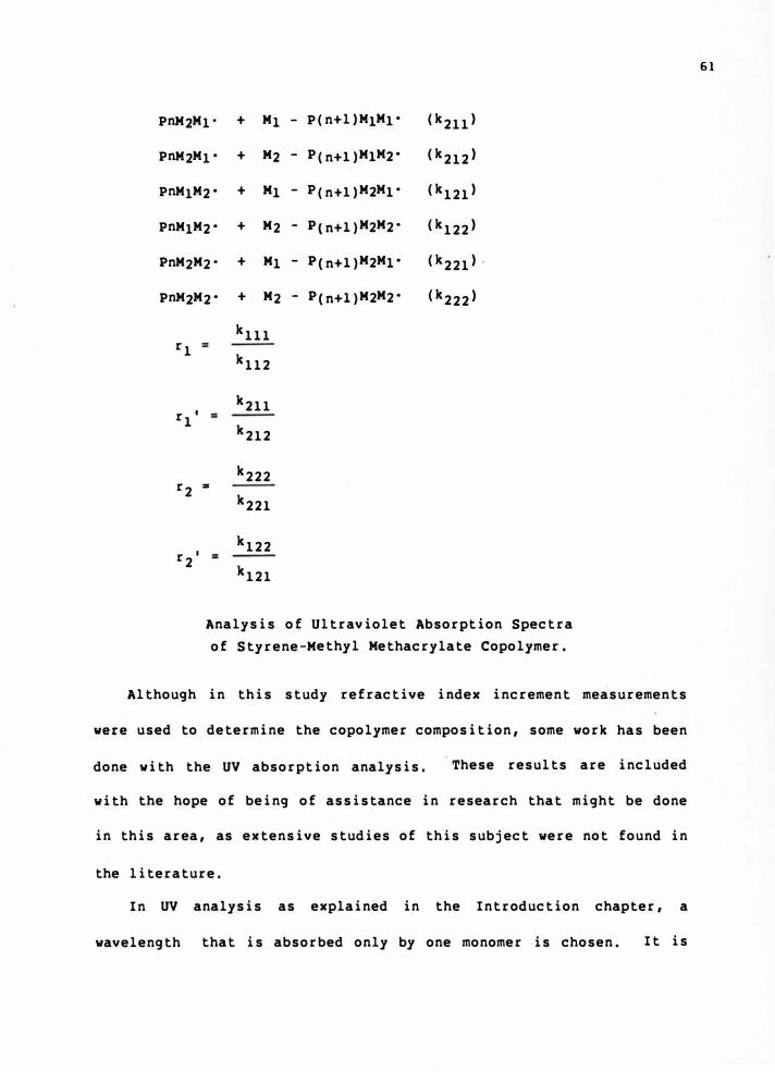
PnM2M1 + M1 - P(n+l)M1M1• (k211>
PnM2M1• + M2 - P(n+1)M1M2• (k212>
PnM1M2• + M1 - P(n+1)M2M1• (k121>
PnM1M2• + M2 - P(n+1)M2M2• (k122>
PnM2M2· + M1 - P(n+1)M2M1• (k221>
PnM2M2• + M2 - P(n+1)M2M2• (k222>
k111 r1
k112
I k211
rl k212
k222 r2
,. k221
I k122
r2 k121
Analysis of Ultraviolet Absorption Spectra of Styrene-Methyl Methacrylate Copolymer.
Although in this study refractive index increment measurements
were used to determine the copolymer composition, some work has been
done with the UV absorption analysis. These results are included
with the hope of being of assistance in research that might be done
in this area, as extensive studies of this subject were not found in
the literature.
In UV analysis as explained in the Introduction chapter, a
wavelength that is absorbed only by one monomer is chosen. It is
61
assumed that the other monomer has neither an absorption nor an
indirect effect on the absorption of the chromophore unit.
Styrene was the chromophore selected in this copolymer, and it
was assumed that absorption by methyl methacrylate uni ts in the
copolymer was negligible.
that have to be considered.
However, there _are some other factors
This aspect can easily be seen by the
significant difference of the absorption versus concentration plots
of pure polystyrene46 and a copolymer of styrene in Figure 12. In
the copolymer the relationship is linear until about thirty-five
percent conversio·n but deviates from there on. The reason is
thought to be that in polystyrene there are many adjacent benzene
rings which will affect the electronic spectrum relative to a
copolymer with isolated benzene rings.
This effect was observed in Figure 13 by overlapping the UV
absorption spectrum of the various monomer feed compositions of
styrene-methyl methacrylate copolymers containing the same concen-
tration of styrene. The spec i fie absorbance of each chromophore
unit will differ depending on other chromophore units in · the
vicinity. This leads to three different situations when monomer
sequence triads are considered. In previous studies 7 only diads
were considered but in this study the use of triads was felt to be a
better choice. These triads can be designated type I, II, and III,
which refer to (BAB), (BAA or AAB) and (AAA) monomer sequences,
respectively. In this case, styrene is the chromophore unit A
and Bis the methyl methacrylate unit. The relative concentrations
62
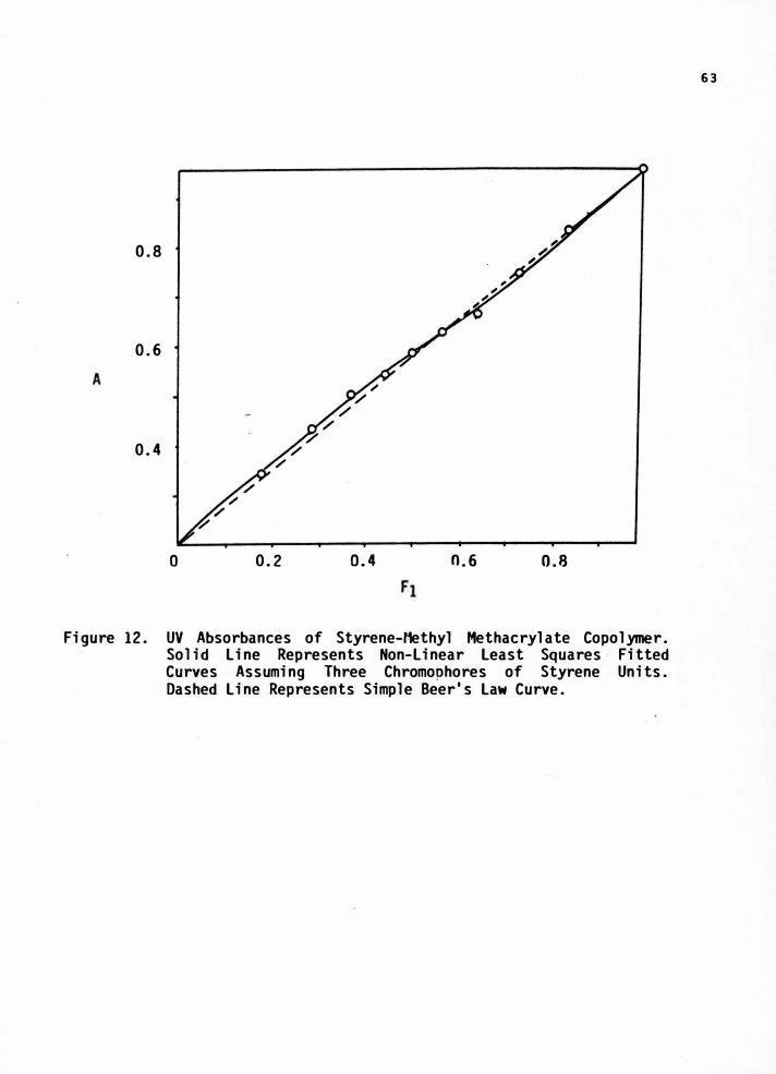
0.8
0.6
0.4
0 0.2 0.4 0.6 0.8
Figure 12. UV Absorbances of Styrene-Methyl Methacrylate Copolymer. Solid Line Represents Non-Linear Least Squares Fitted Curves Assuming Three Chromophores of Styrene Units. Dashed Line Represents Simple Beer's Law Curve.
63

A
3.o,""T--------------------------
1.5
240 260
� {nm)
..
� \;.::-��--- . -· -·..:.;,.�::-�� �-..;..; .___...,_ __
280 300
Figure 13. Overlapped Ultraviolet Absorption of the Various Monomer Feed Compositions of Styrene-Methyl Methacrylate Copolymers All Containing l.Omg/ml of Styrene.

of the three types of units were computed using the overall best
fit values of monomer reactivity ratios, r1 and r2, in the following
formulas,
Fraction type I = (1 - p11)K
Fraction type II = 2 Pu
K
Fraction type III
Pu 2
K
l - Pu
where, P11 is the probability that a growing radical chain M1• will
add to monomer M1, and
Pu =
Then,
and IC = l - Pu
Pu 2
IC = l l - Pu
IC is the normalizing factor, so
Fraction type I • (1 - p11) 2
Fraction type II • 2p11(l - P11>
Fraction type III • p112
Using values of r1 = 0.49520 and r2
= 0.46669, a plot of. the
fraction of each type of triads versus mole percent styrene in
monomer feed can be seen in Figure 14.
Finally the non-linear least square fitted values of the single
wavelength UV absorbances of copolymers were plotted against
concentration. Comparison with the observed absorbance values of
the styrene-methyl methacrylate copolymer was made.
are seen in Table 4 and the plot in Figure 12.
These values
65
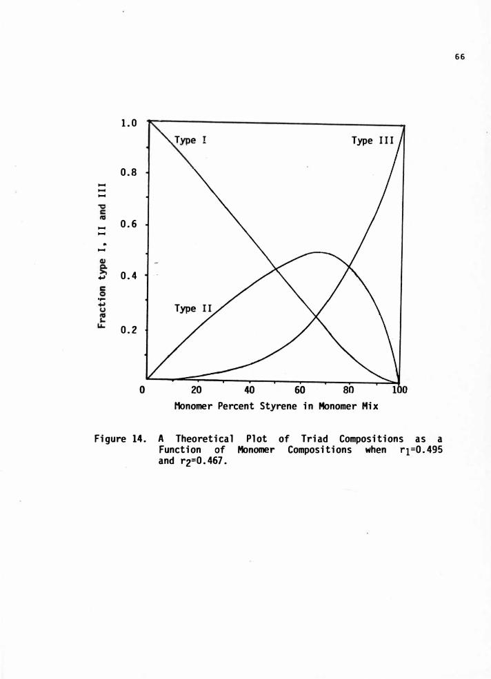
1.0
Type III
0.8 -
-
-
-0.6 -
..
-
0.4 �
.,..
0.2
Monomer Percent Styrene in Monomer Mix
Figure 14. A Theoretical Plot of Triad Compositions as a Function of Monomer Compositions when q=0.495 and r2=0.467.
66
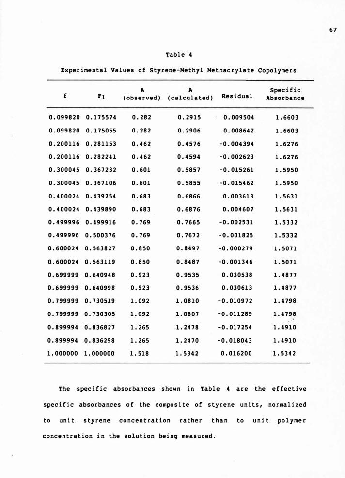
Table 4
Experimental Values of Styrene-Methyl Methacrylate Copolymers
A A Specific f F1 (observed) (calculated) Residual Absorbance
0.099820 0.175574 0.282 0.2915 0.009504 l. 6603
0.099820 0.175055 0.282 0.2906 0.008642 1.6603
o. 200116 0.281153 0.462 0.4576 -0.004394 1.6276
0.200116 0.282241 0.462 0.4594 -0.002623 l. 6276
0.300045 0.367232 0.601 0.5857 -0.015261 1.5950
0.300045 0.367106 0.601 0.5855 -0.015462 1.5950
0.400024 0.439254 0.683 0.6866 0.003613 1.5631
0.400024 0.439890 0.683 0.6876 0.004607 1.5631
0.499996 0.499916 0.769 0.7665 -0. 002531 1.5332
0.499996 0.500376 0.769 0.7672 -0.001825 1.5332
0.600024 0.563827 0.850 0.8497 -0.000279 1.5071
0.600024 0.563119 0.850 0.8487 -0.001346 1.5071
0.699999 0.640948 0.923 0.9535 0.030538 1.4877
0.699999 0.640998 0.923 0.9536 0.030613 1.4877
0.799999 0.730519 1.092 1.0810 -0.010972 1.4798
0.799999 0.730305 1.092 1.0807 -0.011289 1.4798
0.899994 0.836827 1.265 1.2478 -0.017254 1.4910
0.899994 0.836298 1.265 1.2470 -0.018043 1.4910
1.000000 1.000000 l. 518 l. 5342 0.016200 1.5342
The specific absorbances shown in Table 4 are the effective
specific absorbances of the composite of styrene units, normalized
to unit styrene concentration rather than to unit polymer
concentration in the solution being measured.
67
Conclusions
The following conclusions can be derived from the results that
were obtained in this study.
The composition of polymer changed with conversion as expected
for the range of conversion study.
The rate of copolymerization when plotted against monomer
composition gave essentially a J-shaped curve.
The maximum likelihood method is the best method to find the r1
and r2 values. The second best is the Non-Linear Least Squares
method. The Intersection method ranks third, Kelen-Tudos fourth and
Fineman-Ross fifth in accuracy. However, Kelen-Tudos appears to be
a good method for routine determinations because of its simplicity
and accuracy.
The effect of ignoring conversion in the calculations leads to
significant errors in the reactivity ratios, even if the actual
conversion is only a few percent.
In the UV region there appear to be several different
chromophores in this copolymer, so that a simple applicatiorl of
Beer's Law is not valid for determining the composition.
68

Recommendations
In this study all calculations were done assuming the absence of
penultimate unit effects. However the analysis of residuals from
statistical data fitting showed a strong possibility of a
penultimate effect. Therefore, it is recommended that this factor
be considered in further studies to obtain a better fit of
experimental data to the theoretical data.
Another area of consideration is in the method of finding
copolymer compositions with the aid of UV absorbances. In this
study monomer sequence triads were used instead of diads which had
been used in previous studies. Still it was assumed that methyl
methacrylate monomer had no absorption at the wavelength selected.
However, it is possible that methyl methacrylate has an absorption
even though it probably is very small. Calculations including
methyl methacrylate as a chromophore might therefore give more
accurate copolymer composition values.
One other interesting research would be to do this study with
monomers that have a much bigger difference in r1 and r2 va.lues.
This would result in a much larger composition drift. A comparison
of methods to find r1 and r2 with such a copolymer system would
increase the applicability of the results obtained in this research.
69

APPENDICES
70
APPENDIX A
Experimental Data for Copolymerization of
Styrene with Methyl Methacrylate
71
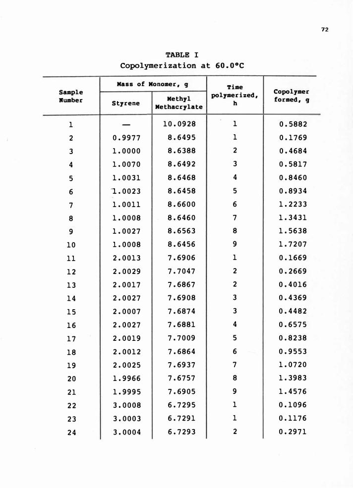
Sample
Wumber
1
2
3
4
5
6
7
8
9
10
11
12
13
14
15
16
17
18
19
20
21
22
23
24
TABLE I
Copolymerization at 60.0°C
Nass of Monomer, g Time
polymerized, Methyl
Styrene Nethacrylate
h
- 10.0928 1
0.9977 8.6495 1
1.0000 8.6388 2
1.0070 8.6492 3
1.0031 8.6468 4
'1..0023 8.6458 5
1.0011 8.6600 6
1.0008 8.6460 7
1.0027 8.6563 8
1.0008 8.6456 9
2.0013 7.6906 1
2.0029 7.7047 2
2.0017 7.6867 2
2.0027 7.6908 3
2.0007 7.6874 3
2.0027 7.6881 4
2.0019 7.7009 5
2.0012 7.6864 6
2.0025 7.6937 7
1.9966 7.6757 8
1.9995 7.6905 9
3.0008 6.7295 1
3.0003 6.7291 1
3.0004 6.7293 2
72
Copolymer
formed, g
0.5882
0.1769
0.4684
0.5817
0.8460
0.8934
1.2233
1.3431
1.5638
1.7207
0.1669
0.2669
0.4016
0.4369
0.4482
0.6575
0.8238
0.9553
1.0720
1.3983
1.4576
0.1096
0.1176
0.2971

73
TABLE !--Continued
Nass of Monomer, g
Sample Time
polymerized, Copolymer
Rumber Methyl h formed, g
Styrene Methacrylate
26 3.0007 6.7295 4 0.5921
27 2.9997 6.7287 4 0.6406
28 3.0007 6.7287 5 0.7407
29 2.9999 6.7286 6 0.9931
30 3.0008 6.7297 7 1.0844
31 _3. 0009 6.7296 8 1.3802
32 · 6.7295 9 1.6215
33 5.7674 1 0.1264
34 5.7679 2 0.2495
35 5.7680 3 0.3732
36 5.7680 4 0.6832
37 5.7681 4 0.4920
38 5.7678 5 0.7435
39 5.7682 5 0.5865
40 5.7680 6 0.7090
41 5.7681 7 0.7573
42 5.7683 7 1.0579
43 5.7679 7 1.0852
44 5.7682 8 1.0250
45 5.7679 9 1.3714
46 5.7677 9 1.3040
47 4.8066 1 0.1217
48 4.8067 2 0.2492
49 4.8067 2 0.2095

74
TABLE !--Continued
Mass of Monomer, g
Sample Time
Copolymer polymerized,
Rumber Methyl h formed, g
Styrene Nethacrylate
51 4.9999 4.8063 4 0.5095
52 5.0002 4.8067 4 0.4504
53 5.0004 4.8069 5 0.5684
54 5.0002 4.8067 6 0.6646
55 5.0001 4.8069 7 0.7709
56 ..5. 0004 4.8067 8 0.8747
57 -S.0000 4.8066 9 0.9697
58 6.0004 3.8451 1 0.1481
59 6.0001 3.8449 1 0.0933
60 6.0000 3.8447 2 0.2029
61 6.0012 3.8454 2 0.1928
62 6.0009 3.8454 3 0.3692
63 6.0011 3.8455 3 0.3042
64 6.0010 3.8451 4 0.4823
65 6.0014 3.8454 4 0.4946
66 6.0008 3.8453 5 0.5959
67 6.0013 3.8455 5 0.5465
68 6.0007 3.8454 6 0.6199
69 6.0012 3.8456 7 0.7837
70 6.0013 3.8455 8 0.8281
71 6.0014 3.8456 9 0.8946
72 6.0008 3.8454 9 1.1034
73 7.0009 2.8843 1 0.1052
74 7.0013 2.8848 2 0.2002
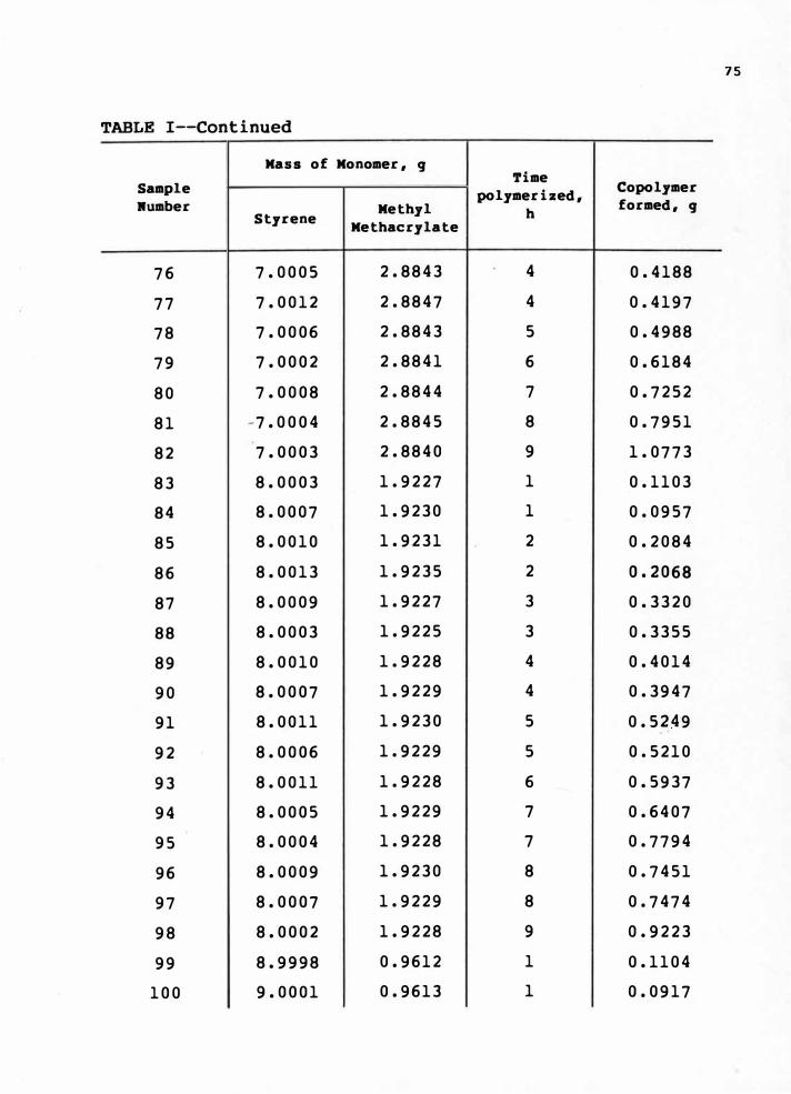
75
TABLE !--Continued
Mass of Monomer, g
Sample Time
Copolymer polymerized,
Kumber Methyl h formed, g
Styrene Methacrylate
76 7.0005 2.8843 4 0.4188
77 7.0012 2.8847 4 0.4197
78 7.0006 2.8843 5 0.4988
79 7.0002 2.8841 6 0.6184
80 7.0008 2.8844 7 0.7252
81 -7. 0004 2.8845 8 0.7951
82 7.0003 2.8840 9 1.0773
83 8.0003 1.9227 1 0.1103
84 8.0007 1.9230 1 0.0957
85 8.0010 1.9231 2 0.2084
86 8.0013 1.9235 2 0.2068
87 8.0009 1.9227 3 0.3320
88 8.0003 1.9225 3 0.3355
89 8.0010 1.9228 4 0.4014
90 8.0007 1.9229 4 0.3947
91 8.0011 1.9230 5 0.5��9
92 8.0006 1.9229 5 0.5210
93 8.0011 1.9228 6 0.5937
94 8.0005 1.9229 7 0.6407
95 8.0004 1.9228 7 0.7794
96 8.0009 1.9230 8 0.7451
97 8.0007 1.9229 8 0.7474
98 8.0002 1.9228 9 0.9223
99 8.9998 0.9612 1 0.1104
100 9.0001 0.9613 1 0.0917

76
TABLE !--Continued
Mass of Monomer, g
Sample Time
Copolymer polymerized,
Wwaber Methyl h formed, g
Styrene Methacrylate
101 9.0003 0.9614 1 0.0950
102 9.0005 0.9615 2 0.2425
103 9.0010 0.9616 2 0.1940
104 9.0006 0.9614 3 0.3159
105 9.0002 0.9612 4 0.4207
106 -9.0003 0.9613 4 0.4716
107 9.0002 0.9614 5 0.5972
108 9.0008 0.9615 5 0.5960
109 9.0001 0.9614 5 0.5527
110 9.0010 0.9617 6 0.6967
111 9.0004 0.9614 7 0.8119
112 9.0003 0.9615 7 0.8129
113 9.0009 0.9616 8 0.8443
114 9.0004 0.9615 8 0.9035
115 9.0011 0.9617 9 1.0616
116 10.1281 - 1 0.1439

TABLE II
Differential Refractive Index Increments
Sample Number
1
2
3
4
5
6
7
8
9
10
11
12
13
14
15
16
17
18
19
20
21
22
23
24
25
dn/dcin Methyl Ethyl
Ketone
0.1200
0.1385
0.1384
0.1383
0.1384
0.1383
0.1383
0.1382
0.1382
0.1380
0.1495
0.1495
0.1494
0.1494
0.1493
0.1494
0.1493
0.1493
0.1492
0.1491
0.1489
0.1584
0.1583
0.1583
0.1582
dn/dcin Ethyl Acetate
0.1177
0.1362
0.1361
0.1360
0.1360
0.1359
0.1358
0.1357
0.1356
0.1355
0.1474
0.1473
0.1473
0.1472
0.1473
0.1472
0.1471
0.1471
0.1470
0.1468
0.1467
0.1562
0.1561
0.1560
0.1561
77

78
TABLE II--Continued
Sample dn/dc dn/dc
Number in Methyl Ethyl in Ethyl Acetate
Ketone
26 0.1582 0.1560
27 0.1582 0.1559
28 0.1581 0.1559
29 0.1581 0.1558
30 0.1580 0.1557
31 -
0.1579 0.1556
32 0.1578 0.1555
33 0.1658 0.1637
34 0.1657 0.1636
35 0.1656 0.1635
36 0.1657 0.1635
37 0.1656 0.1634
38 0.1656 0.1634
39 0.1655 0.1633
40 0.1655 0.1633
41 0.1654 0.1631
42 0.1653 0.1630
43 0.1653 0.1630
44 0.1653 0.1630
45 0.1653 0.1629
46 0.1653 0.1629
47 0.1720 0.1699
48 0.1719 0.1699
49 0.1719 0.1699
50 0.1720 0.1699
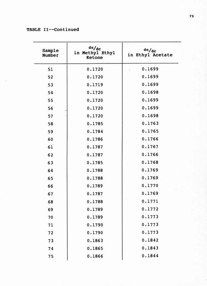
79
TABLE !!--Continued
Sample dn/dc dn/dc
Number in Methyl Ethyl
in Ethyl Acetate Ketone
51 0.1720 0.1699
52 0.1720 0.1699
53 0.1719 0.1699
54 0.1720 0.1698
55 0.1720 0.1699
56 0.1720 0.1699
57 0.1720 0.1698
58 0.1785 0.1763
59 0.1784 0.1765
60 0.1786 0.1766
61 0.1787 0.1767
62 0.1787 0.1766
63 0.1785 0.1768
64 0.1788 0.1769
65 0.1788 0.1769
66 0.1789 0.1770
67 0.1787 0.1769
68 0.1788 0.1771
69 0.1789 0.1772
70 0.1789 0.1773
71 0.1790 0.1773
72 0.1790 0.1773
73 0.1863 0.1842
74 0.1865 0.1843
75 0.1866 0.1844

80
TABLE !!--Continued
Sample dn/dc dn/dc
Number in Methyl Ethyl in Ethyl Acetate
Ketone
76 0.1868 0.1845
77 0.1868 0.1845
78 0.1869 0.1845
79 0.1870 0.1846
80 0.1870 0.1847
81 0.1871 0.1848
82 0.1872 0.1849
83 0.1953 0.1932
84 0.1953 0.1932
85 0�1954 0.1933
86 0.1955 0.1934
87 0.1955 0.1934
88 0.1956 0.1935
89 0.1956 0.1935
90 0.1956 0.1935
91 0.1957 0.1936
92 0.1958 0.1937
93 0.1957 0.1937
94 0.1958 0.1937
95 0.1959 0.1938
96 0.1959 0.1938
97 0.1959 0.1938
98 0.1960 0.1939
99 0.2059 0.2038
100 0.2059 0.2038
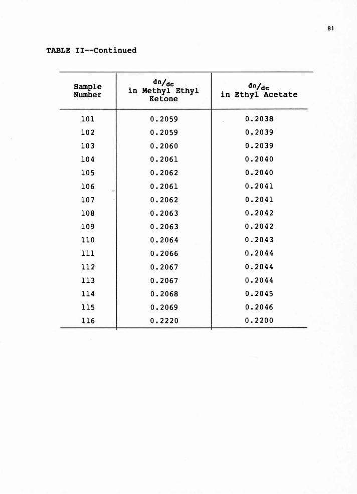
81
TABLE II--Continued
Sample dn/dc dn/dc
Number in Methyl Ethyl
in Ethyl Acetate Ketone
101 0.2059 0.2038
102 0.2059 0.2039
103 0.2060 0.2039
104 0.2061 0.2040
105 0.2062 0.2040
106 0.2061 0.2041
107 0.2062 0.2041
108 0.2063 0.2042
109 0.2063 0.2042
110 0.2064 0.2043
111 0.2066 0.2044
112 0.2067 0.2044
113 0.2067 0.2044
114 0.2068 0.2045
115 0.2069 0.2046
116 0.2220 0.2200
APPENDIX 8
Calculated Values of Composition and Conversion
for Copolymerization of Styrene
with Methyl Methacrylate
82

83
TABLE I
Conversion as a Function of Time of Polymerization at 60.0°C
Sample Percent Percent Time of
Covers ion Conversion Polymerization, Number
by mass by mole h
1 1.4207 1
2 1.8367 1.8281 1
3 4.8595 4.8451 2
4 6.0241 6.0065 3
5 8.7671 8.7409 4
6 9.2600 9.2327 5
7 12.6621 12.6248 6
8 13.9228 13.8826 7
9 16.1901 16.1431 8
10 17.8377 17.7873 9
11 1.7221 1.7165 1
12 2.7494 2.7405 2
13 4.1452 4.1320 2
14 4.5071 4.4928 3
15 4.6263 4.6117 3
16 6.7848 6.7632 4
17 8.4903 8.4635 5
18 9.8611 9.8300 6
19 11.0559 11. 0215 7
20 14.4567 14.4123 8
21 15.0423 14.9971 9
22 1.1264 1.1234 1
23 1.2087 1.2055 1
24 3.0535 3.0455 2
25 4.6763 4.6641 3

84
TABLE I--Continued
Sample Percent Percent Time of
Covers ion Conversion Polymerization, Number by mass by mole h
26 6.0852 6.0694 4
27 6.5848 6.5678 4
28 7.6130 7.5936 5
29 10.2082 10.1821 6
30 11.1443 11.1163 7
31 14.1843 14.1492 8
32 -16.6655 16.6249 9
33 1.2941 1.2921 1
34 2.5542 2.5503 2
35 3.8205 3.8149 3
36 6.9937 6.9831 4
37 5.0365 5.0291 4
38 7.6119 7.6007 5
39 6.0037 5.9951 5
40 7.2582 7.2477 6
41 7.7525 7.7417 7
42 10.8293 10.8145 7
43 11.1099 11.0947 7
44 10.4928 10.4785 8
45 14.0397 14.0206 9
46 13.3503 13.7616 9
47 1. 2410 1.2410 1
48 2.5411 2.5412 2
49 2.1363 2.1364 2
50 3.6606 3.6606 3
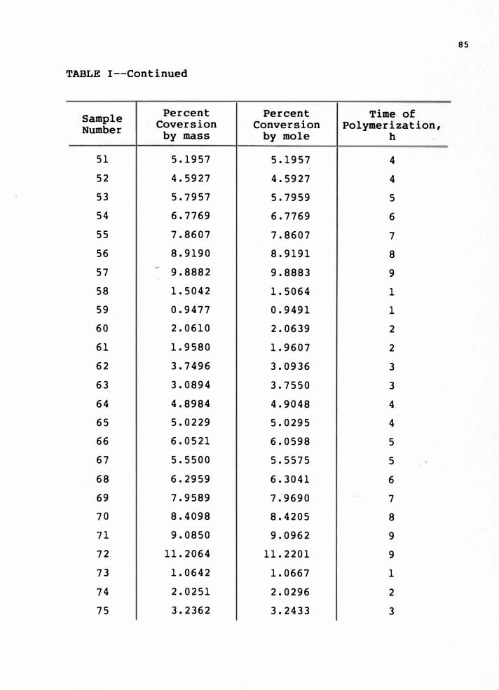
85
TABLE !--Continued
Sample Percent Percent Time of
Covers ion Conversion Polymerization, Number by mass by mole h
51 5.1957 5.1957 4
52 4.5927 4.5927 4
53 5.7957 5.7959 5
54 6.7769 6.7769 6
55 7.8607 7.8607 7
56 8.9190 8.9191 8
57 9.8882 9.8883 9
58 1.5042 1.5064 1
59 0.9477 0.9491 1
60 2.0610 2.0639 2
61 1.9580 1.9607 2
62 3.7496 3.0936 3
63 3.0894 3.7550 3
64 4.8984 4.9048 4
65 5.0229 5.0295 4
66 6.0521 6.0598 5
67 5.5500 5.5575 5
68 6.2959 6.3041 6
69 7.9589 7.9690 7
70 8.4098 8.4205 8
71 9.0850 9.0962 9
72 11.2064 11.2201 9
73 1.0642 1.0667 1
74 2.0251 2.0296 2
75 3.2362 3.2433 3
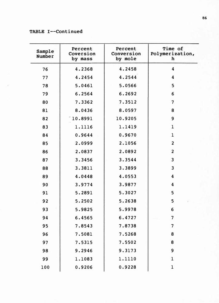
86
TABLE !--Continued
Sample Percent Percent Time of
Covers ion Conversion Polymerization, Number
by mass by mole h
76 4.2368 4.2458 4
77 4.2454 4.2544 4
78 5.0461 5.0566 5
79 6.2564 6.2692 6
80 7.3362 7.3512 7
81 8.0436 8.0597 8
82 - 10. 8991 10.9205 9
83 1.1116 1.1419 1
84 0.9644 0.9670 1
85 2.0999 2.1056 2
86 2.0837 2.0892 2
87 3.3456 3.3544 3
88 3.3811 3.3899 3
89 4.0448 4.0553 4
90 3.9774 3.9877 4
91 5.2891 5.3027 5
92 5.2502 5.2638 5
93 5.9825 5.9978 6
94 6.4565 6.4727 7
95 7.8543 7.8738 7
96 7.5081 7.5268 8
97 7.5315 7.5502 8
98 9.2946 9.3173 9
99 1.1083 1.1110 1
100 0.9206 0.9228 1

87
TABLE !--Continued
Sample Percent Percent Time of
Covers ion Conversion Polymerization, Number
by mass by mole h
101 0.9537 0.9560 1
102 2.4343 2.4402 2
103 1.9473 1.9520 2
104 3.1710 3.1786 3
105 4.2233 4.2332 4
106 4.7341 4.7455 4
107 5.9950 6.0091 5
108 5.9826 5.9963 5
109 5.5484 5.5611 5
110 6.9931 7.0089 6
111 8.1501 8.1679 7
112 8.1602 8.1777 7
113 8.4748 8.4929 8
114 9.0696 9.0886 8
115 10.6556 10.6776 9
116 5.8279 - 1

88
TABLE II
Concentration of Styrene Units in the Monomer Feed and in the Styrene-Methyl Methacrylate Copolymer
Styrene in Styrene in Copolymer Monomer
From dn/dc From dn/dc
Sample Measurements in Measurements in
Number Methyl Ethyl Ketone Ethyl Acetate
mass mole mass mole mass mole fraction fraction fraction fraction fraction fraction
z 0 1
f 0 1 ][l Fl Xl Fl
1 0.0000 0.0000
2 0.1034 0.0998 0.1814 0.1756 0.1808 0.1751
3 0 .1037 0.1001 0.1804 0.1746 0.1799 0.1741
4 0.1043 0.1007 0.1794 0.1737 0.1789 0.1731
5 0.1039 0.1003 0.1804 0.1746 0.1789 0.1731
6 0.1039 0.1003 0.1794 0.1737 0.1779 0.1722
7 0.1036 0.1000 0.1794 0.1737 0.1769 0.1712
8 0.1037 0.1001 0.1784 0.1727 0.1760 0.1703
9 0.1038 0.1002 0.1784 0.1727 0.1750 0.1693
10 0.1037 0.1001 0.1764 0.1708 0.1740 0.1684
11 0.2065 0.2001 0.2892 0.2812 0.2903 0.2822
12 0.2063 0.1999 0.2892 0.2812 0.2893 0.2813
13 0.2066 0.2002 0.2882 0.2802 0.2893 0.28.13
14 0.2066 0.2002 0.2882 0.2802 0.2884 0.2803
15 0.2065 0.2001 0.2873 0.2792 0.2893 0.2813
16 0.2067 0.2003 0.2882 0.2802 0.2884 0.2803
17 0.2063 0.1999 0.2873 0.2792 0.2874 0.2794
18 0.2066 0.2002 0.2873 0.2792 0.2874 0.2794
19 0.2065 0.2001 0.2863 0.2783 0.2864 0.2784
20 0.2064 0.2000 0.2853 0.2773 0.2845 0.2765

89
TABLE II--Continued
Styrene in Styrene in Copolymer Monomer
From dn/dc From dn/dc
Sample Measurements in Measurements in
Number Methyl Ethyl Ketone Ethyl Acetate
mass mole mass mole mass mole
fraction fraction fraction fraction fraction fraction JI 0
1 f 0 1 Xl
Fl X1 Fl
21 0.2063 0.1999 0.2833 0.2754 0.2835 0.2755
22 0.3084 0.3000 0.3765 0.3672 0.3763 0.3671
23 0.3084 0.3000 0.3755 0.3662 0.3754 0.3661
24 0.308� 0.3000 0.3755 0.3663 0.3744 0.3652
25 0.3084 0.3000 0.3745 0.3653 0.3754 0.3661
26 0.3084 0.3000 0.3745 0.3653 0.3744 0.3652
27 0.3083 0.2999 0.3745 0.3653 0.3734 0.3642
28 0.3084 0.3001 0.3735 0.3643 0.3734 0.3642
29 0.3084 0.3000 0.3735 0.3643 0.3724 0.3632
30 0.3084 0.3000 0.3725 0.3634 0.3715 0.3623
31 0.3084 0.3000 0.3716 0.3624 0.3705 0.3613
32 0.4095 0.4000 0.3706 0.3614 0.3695 0.3603
33 0.4095 0.4000 0.4490 0.4393 0.4497 0.4399
34 0.4095 0.4000 0.4480 0.4383 0.4487 0.4389
35 0.4095 0.4000 0.4471 0.4373 0.4477 0.4379
36 0.4095 0.4000 0.4480 0.4383 0.4477 0.4379
37 0.4095 0.4000 0.4471 0.4373 0.4467 0.4370
38 0.4095 0.4000 0.4471 0.4373 0.4467 0.4370
39 0.4095 0.4000 0.4461 0.4363 0.4457 0.4360
40 0.4095 0.4000 0.4461 0.4363 0.4457 0.4360

90
TABLE II--Continued
Styrene in Styrene in Copolymer Monomer
Prom dn/dc Prom dn/dc
Sample Measurements in Measurements in
Number Methyl Ethyl Ketone Ethyl Acetate
mass mole mass mo·le mass mole fraction fraction fraction fraction fraction fraction
JI: 0
1 f 0 1 11 pl 11 pl
41 0.4095 0.4000 0.4451 0.4354 0.4438 0.4341
42 0.4095 0.4000 0.4441 0.4344 0.4428 0.4331
43 0.4095 0.4000 0.4441 0.4344 0.4428 0.4331
44 0.4095 0.4000 0.4441 0.4344 0.4428 0.4331
45 0.4095 0.4000 0.4441 0.4344 0.4418 0.4321
46 0.5099 0.5000 0.4441 0.4344 0.4418 0.4321
47 0.5099 0.5000 0.5098 0.4999 0.5103 0.5004
48 0.5099 0.5000 0.5088 0.4989 0.5103 0.5004
49 0.5099 0.5000 0.5088 0.4989 0.5103 0.5004
50 0.5099 0.5000 0.5098 0.4999 0.5103 0.5004
51 0.5099 0.5000 0.5098 0.4999 0.5103 0.5004
52 0.5099 0.5000 0.5098 0.4999 0.5103 0.5004
53 0.5099 0.5000 0.5088 0.4989 0.5103 0.5004
54 0.5099 0.5000 0.5098 0.4999 0.5093 0.4994
55 0.5099 0.5000 0.5098 0.4999 0.5103 0.5004
56 0.5099 0.5000 0.5098 0.4999 0.5103 0.5004
57 0.5099 0.5000 0.5098 0.4999 0.5093 0.4994
58 0.6095 0.6000 0.5735 0.5638 0.5728 0.5631
59 0.6095 0.6000 0.5725 0.5628 0.5748 0.5651
60 0.6095 0.6000 0.5745 0.5648 0.5757 0.5661

91
TABLE II--Continued
Styrene in Styrene in Copolymer Monomer
From dn/dc Prom dn/dc
Sample Measurements in Measurements in
Number Methyl Ethyl Ketone Ethyl Acetate
mass mole mass mole mass mole
fraction fraction fraction fraction fraction fraction
z 0
1 f 0
1 X1 "1 X1 "1
61 0.6095 0.6000 0.5755 0.5658 0.5757 0.5661
62 0.6095 0.6000 0.5755 0.5658 0.5757 0.5661
63 0.6095 0.6000 0.5735 0.5638 0.5777 0.5680
64 0. 609.5 0.6000 0.5765 0.5668 0.5787 0.5690
65 0.6095 0.6000 0.5765 0.5668 0.5787 0.5690
66 0.6095 0.6000 0.5774 0.5678 0.5797 0.5700
67 0.6095 0.6000 0.5755 0.5658 0.5787 0.5690
68 0.6095 0.6000 0.5765 0.5668 0.5806 0.5710
69 0.6095 0.6000 0.5774 0.5678 0.5816 0.5720
70 0.6095 0.6000 0.5774 0.5678 0.5826 0.5730
71 0.6095 0.6000 0.5784 0.5687 0.5826 0.5730
72 0.6095 0.6000 0.5784 0.5687 0.5826 0.5730
73 0.7082 0.7000 0.6500 0.6409 0.6500 0.6410
74 0.7082 0.7000 0.6520 0.6429 0.6510 0.6420
75 0.7082 0.7000 0.6530 0.6439 0.6520 0.6430
76 0.7082 0.7000 0.6550 0.6459 0.6530 0.6440
77 0.7082 0.7000 0.6550 0.6459 0.6530 0.6440
78 0.7082 0.7000 0.6560 0.6568 0.6530 0.6440
79 0.7082 0.7000 0.6570 0.6479 0.6540 0.6450
80 0.7082 0.7000 0.6570 0.6479 0.6549 0.6460

92
TABLE II--Continued
Styrene in Styrene in Copolymer Monomer
From dn/dc From dn/dc
Sample Measurements in Measurements in
Number Methyl Ethyl Ketone Ethyl Acetate
mass mole mass mole mass mole fraction fraction fraction fraction fraction fraction
Jl 0 1 f 0 1 11 Fl 11 F1
81 0.7082 0.7000 0.6580 0.6489 0.6559 0.6470
82 0.7082 0.7000 0.6590 0.6499 0.6569 0.6480
83 0.8062 0.8000 0.7382 0.7305 0.7380 0.7303
84 0.80�2 0.8000 0.7382 0.7305 0.7380 0.7303
85 0.8062 0.8000 0.7392 0.7315 0.7390 0.7313
86 0.8062 0.8000 0.7402 0.7325 0.7400 0.7323
87 0.8062 0.8000 0.7402 0.7325 0.7400 0.7323
88 0.8062 0.8000 0.7412 0.7335 0.7410 0.7333
89 0.8062 0.8000 0.7412 0.7335 0.7410 0.7333
90 0.8062 0.8000 0.7412 0.7335 0.7410 0.7333
91 0.8062 0.8000 0.7422 0.7345 0.7420 0.7343
92 0.8062 0.8000 0.7431 0.7355 0.7430 0.7353
93 0.8062 0.8000 0.7422 0.7345 0.7430 0.7353
94 0.8062 0.8000 0.7431 0.7355 0.7430 0.7353
95 0.8062 0.8000 0.7441 0.7365 0.7439 0.7363
96 0.8062 0.8000 0.7441 0.7365 0.7439 0.7363
97 0.8062 0.8000 0.7441 0.7365 0.7439 0.7363
98 0.8062 0.8000 0.7451 0.7375 0.7449 0.7373
99 0.9035 0.9000 0.8422 0.8368 0.8416 0.8363
100 0.9035 0.9000 0.8422 0.8368 0.8416 0.8363

93
TABLE II--Continued
Styrene in Styrene in Copolymer Monomer
Prom dn/dc Prom dn/dc
Sample Measurements in Measurements in
Number Methyl Ethyl Ketone Ethyl Acetate
mass mole mass mole mass mole
fraction fraction fraction fraction fraction fraction :I: 0
1 f 0 1 X1 pl X1 Pl
101 0.9035 0.9000 0.8422 0.8368 0.8416 0.8363
102 0.9035 0.9000 0.8422 0.8368 0.8426 0.8373
103 0.9035 0.9000 0.8431 0.8378 0.8426 0.8373
104 0.9035 0.9000 0.8441 0.8388 0.8436 0.8383
105 0.9035 0.9000 0.8451 0.8398 0.8436 0.8383
106 0.9035 0.9000 0.8441 0.8388 0.8446 0.8393
107 0.9035 0.9000 0.8451 0.8398 0.8446 0.8393
108 0.9035 0.9000 0.8461 0.8409 0.8456 0.8403
109 0.9035 0.9000 0.8461 0.8409 0.8456 0.8403
110 0.9035 0.9000 0.8471 0.8419 0.8465 0.8413
111 0.9035 0.9000 0.8490 0.8439 0.8475 0.8423
112 0.9035 0.9000 0.8500 0.8449 0.8475 0.8423
113 0.9035 0.9000 0.8500 0.8449 0.8475 0.8423
114 0.9035 0.9000 0.8510 0.8459 0.8485 0.84'33
115 0.9035 0.9000 0.8520 0.8469 0.8495 0.8443
116 1.0000 1. 0000

REFERENCES
1. Billmeyer, F. W. "Textbook of Polymer Science", 2nd ed., New York: Interscience, 1971, Chapter 11.
2. Wall, F. T. The Structure of Vinyl Copolymers. J. Am. Chem.Soc., 1941, 63, 1862-1870.
3. Mayo, F. R., and Lewis, F. M. A Basis for Comparing the Behavior of Monomers in Copolymerization; The Copolymerization of Styrene and Methyl Methacrylate. J. Am. Chem. Soc., 1944, 66, 1594-1601.
4. Alfrey, T., and Goldfinger, G. The Mechanism of Copolymerization. J. Phys. Chem., 1944, 12, 205-210.
5. Critchfield, F. E., and Johnson, D. P. Chemical Analysis ofPolymers.- Anal. Chem., 1961, 33, 1834-1836.
6. Funt, B. L., and Collins, E. Formation of Block Polymers ofButyl Acrylate with Styrene and Vinyl Pyridine. J. Polym. Sci., 1958, 28, 359-364.
7. Tobolsky, A. v., Eisenberg, A., and O'Driscoll, K. F. Spectrophotometric Determination of Styrene in a Styrene-Methyl Methacrylate Copolymer. Anal. Chem., 1959, 1!, 203-204.
8. O'Driscoll, K. F., Wertz, W., and Husar, A. Influence of Intrachain Interactions on the Kinetics of Styrene Polymerization and Copolymerization. J. Polym. Sci., 1967, SA, 2159-2166.
9. Brussau, R. J., and Stein, D. J. Abhangigkeit der UV-Absorptionbinarer Styrol-Copolymerisate von der Lange der Styrolsequenzen. Angew. Macromol. Chem., 1970, 12, 59-71.
10. Gallo, B. M., and Russo, S. Ultraviolet Absorption Spectra ofStyrene Copolymers. I. Solvent Effects on the Hypochromism of Poly(Styrene-co-Methyl Methacrylate) at 2695 A0 •
J. Macromol. Sci.-Chem., 1974, AS, 521-531.
11. Gallo, B. M., and Russo, S. Structure and Properties of Random,Alternating, and Block Copolymers: The UV Spectra of Styrene-Methyl Methacrylate Copolymers. Adv. Chem. Ser., 1975, 142, 85-91.
12. Stutzel, B., Miyamoto, T., and Cantow, H. J. HypochromicEffects in UV Spectra of Polymers in Solution. Polym. J., 1976, !, 247-253.
13. Gruber, E., and Knell, w. L. Bestimmung der Chemischen Heterogenitat Statistischer Copolymerer anhand von Untersuchungen and Poly(Styrol-co-Butyl Acrylat) und Poly(Styrol-co-Butyl Methacrylat). Macromol. Chem., 1978, 179, 733-746.
94

14. Runyon, J. R., Barnes, D. E., Rudd, J. F., and Tung, L. H.Multiple Detectors for Molecular Weight and Composition Analysis of Copolymers by Gel Permeation Chromatography. J. Appl. Polym. Sci., 1969, 13, 2359-2369.
15. Johnson, M., Karmo, T. S., and Smith, R. R. High ConversionCopolymerization of Styrene with Methyl Methacrylate. Eur. Polym. J,, 1978, 14, 409-414.
16. Dionisio, J. M., and O'Driscoll, K. F. High-Conversion Copolymerization of Styrene and Methyl Methacrylate. J. Polym. Sci., Polym. Lett. Ed., 1979, 17, 701-707.
17. Garcia-Rubio, L. H. The Effect of Composition, Sequence Length,and Tacticity on the UV Absorption Analysis of Styrene Copolymers in Solution. J. Appl. Polym. Sci., 1982, 27, 2043-2052.
18. Colthup, N. B., Daly, L. H., and Wiberly, S. E. "Introductionto Infrared and Raman Spectroscopy" New York: Academic Press, 1964, Chapter 13.
19. Bellamy, L. s. "The Infrared Spectra of Complex Molecules", London: Chapman and Hall Ltd., 1975, Chapter 5.
20. Dollish, F. R., and Fateley, W. G. "Characteristic RamanFrequencies of Organic Compound", New York: John Wiley and Sons, 1974, Chapter 6.
21. Angood, A. C., and Koenig, J. L. Effect of Nonrandom PolymerChain Orientation in the Thickness Direction on Infrared Absorption Measurements. Macromolecules, 1969, 1, 37-42.
22. Bovey, F. A. "High Resolution NMR of Macromolecules", New York:Academic Press, 1972, Chapter 4.
23. Barrall, E. M., Contow, M. J. R., and Johnson, J. F. Variationof Refractive Index of Polystyrene with Molecular Weight: Effect on the Determination of Molecular Weight Distributions. J. Appl. Polym. Sci., 1968, 12, 1373-1377.
24. Francois, J., Candow, F., and Benoit, H. Effect of MolecularWeight on the Partial Specific Volume of Polystyrenes in Solution. Polymer, 1974, !§., 618-626.
25. Stockmayer, w. H., Moore, L. D.,Copolymers in Dilute Solution. Styrene-Methyl Methacrylate. 530.
Fixman, M., and Epstein, B. N.
I. Preliminary Results forJ, Polym. Sci., 1955, 16, 517-
26. Bushuk, w., and Benoit, H. Light-scattering Studies ofCopolymers. 1. Effect of Heterogeneity of Chain Composition on the Molecular Weight. Can. J. Chem., 1958, 36, 1616-1626.
95

27. Krause, S. Light Scattering of Copolymers. I. The CompositionDistribution of a Styrene-Methyl Methacrylate Block Copolymer. J. Phys. Chem., 1961, 65, 1616-1623.
28. "Brice-Phoenix Visual Differential Refractometer Catalog" TheVirtis Company, Inc., New York.
29. Ham, G. E. Reactivity of Polar Monomers in Copolymerization.J. Polym. Sci., 1954, 14, 87-93.
30. Fineman, M., and Ross, S. D. Linear Method for DeterminingMonomer Reactivity Ratios in Copolymerization. J. Polym. Sci., 1950, �. 259-265.
31. Kelen, T., and Tiidos, F. Analysis of the Linear Methods forDetermining Copolymerization Reactivity Ratios. I. A New
Improved Linear Graphic Method. J. Macromol. Sci.-Chem., 1975, 179� 1-27.
32. Skeist, I. Copolymerization: The Composition DistributionJ. Am. Chem. Soc., 1946, 68, 1781-1784. Curve.
33. Meyer, V. E., and Lowry, G. G. Integral and Differential BinaryJ. Polym. Sci., 1965, 3A, 2843-Copolymerization Equations.
2851.
34. Kruse, R. L. The Simplified Calculation of Average CopolymerComposition Versus Extent of Polymeriation. J. Polym. Sci., Polymer Letters, 1967, �. 437-440.
35.
36.
37.
Briggs, E. R., and Effects of Temperature
Ratios. J. Am. Chem.
Lewis, F. M., Walling, C., Cumming, W.,
Mayo, F. R. Copolymerization. IV. and Solvents on Monomer Reactivity Soc., 1948, 70, 1519-1423.
Lewis, F. M., Mayo, F. R., and Hulse, W. F. Copolymerization, II. The Copolymerization of Acrylonitrile, MethylMethacrylate, Styrene and Vinylidene Chloride. J. Am. Chem.Soc., 1945, 67, 1701-1705.
Wiley, R. H., and Sale, E. E. Tracer Techniques for the Determination of Monomer Reactivity Ratios. I. A Direct Counting Technique Applied to the Styrene-Methacrylate Copolymerization. J. Polym. Sci., 1960, 42, 479-489.
38. Price, C. C., and Walsh, J. G. Effect of Dielectric SolventJ. Polym. Sci., 1951, �. 239-Medium on Copolymerization.
242.
39. Meyer, V. E. Copolymerization of Styrene and Methyl Methacrylate Reactivity Ratios from Conversion-Composition Data.
J. Polym. Sci. A.l., 1966, !, 2819-2830.
96

40. Lewis, F. M., and Mayo, F. R. Precise Method for Isolation ofHigh Polymers. J. Anal. Chem., 1945, !, 134-136.
41. Timmermans, J. "Physico-Chemical Constants of Pure Organic Compounds." New York:Elsevier Publishing Co. 1950, 361, 415-416.
42. Lowry, G. G., and Kana'an, S. A. "Statistical Treatment ofExperimental Errors in Physical Chemistry Laboratory Supliment" Western Michigan Universi�y.
43. Walling, C. Overall Rates in Copolymerization. Polar Effectsin Chain Initiation and Termination. J. Am. Chem. Soc., 1949, l!, 1930-1935.
44. Ham, G. E. "Copolymerization" New York: Interscience, 1964,
Chapter 1.
45. Merz, E., Alfrey, T., and Goldfinger, G. IntramolecularReaction in Vinyl Polymers as a Means of Investigation of the Propagation Step. J. Polym. Sci., 1946, !, 75-83.
46. Newel, J. E. Residual Monomer in Polystyrene. Anal. Chem.,1951, 23, 445-447.
97


![Partitioned Polymerization VII/ Seeded Emulsion ...partitioned polymerization [11] was applied to the former system, i.e. for discussion of experimental results obtained for methyl](https://img.pdfslide.us/doc/110x75/60ece6a641172d2d2670147d/partitioned-polymerization-vii-seeded-emulsion-partitioned-polymerization-11.jpg)