EFFECT OF FRICTION ON THE ZEL’DOVICH{VON …

EFFECT OF FRICTION ON THE ZEL’DOVICH–VON NEUMANN–DORING

TO CHAPMAN–JOUGUET TRANSITION

by

SUSHMA RAO

Presented to the Faculty of the Graduate School of

The University of Texas at Arlington in Partial Fulfillment

of the Requirements

for the Degree of

MASTER OF SCIENCE IN AEROSPACE ENGINEERING

THE UNIVERSITY OF TEXAS AT ARLINGTON

August 2010

Copyright c© by Sushma Rao 2010

All Rights Reserved

To Pratik, my mother and my sister

ACKNOWLEDGEMENTS

At the culmination of my Master’s thesis, I would like to thank everyone who

inspired and guided me throughout my research.

Firstly, I would like to thank my advisor Dr Frank Lu for believing in me and

giving me the opportunity to do original research. I am extremely grateful for his

constant guidance. I would also like to thank Dr Donald Wilson for his guidance and

support.

Though speaking about my mother’s contribution in my thesis would be a very

small acknowledgement to her influence on me, I believe that the choices she made

and the life that she led set a very high standard for me to try and reach. She was

a constant motivation and emotional support during all my graduate life. To say the

least I owe her my utmost respect .

I would also like to acknowledge here, the wall who stood next to me throughout

my struggles was my now husband Pratik Donde. He not only stood by but was also

was a very integral part of my eternal struggles during the years of graduate life and

particularly my thesis research. His constant nudge kept me going and no words can

describe my gratitude. My mentor and my worst critique lead me through the various

ups and downs of my thesis and graduate studies.

I would also like to thank my sister for always encouraging me in my endeavors.

She was quintessential elder sister who pushed me to reach higher and last longer.

I would also like to thank Eric M. Braun for his help for the Cantera coding

and also Ronnachai Vutthivithayarak for his cheerfull help and support.

May 28, 2010

iv

ABSTRACT

EFFECT OF FRICTION ON THE ZEL’DOVICH–VON NEUMANN–DORING

TO CHAPMAN–JOUGUET TRANSITION

Sushma Rao, MS

The University of Texas at Arlington, 2010

Supervising Professor: Dr. Frank Lu

Detonation theory proposes Chapman-Jouguet state of equilibrium due to the

sonic speed of the products relative to the wave. Experimental observations however

indicated the existence of a sub-Chapman-Jouguet state. The dissertaion proposes

that friction plays a role in defining such a sub-optimal state in detonation wave

propagation in ducts. The problem is addressed analytically by decoupling the friction

losses from the chemical reactions. The non-equilibrium conditions associated with

detonation is modeled by detailed chemistry.

v

TABLE OF CONTENTS

ACKNOWLEDGEMENTS . . . . . . . . . . . . . . . . . . . . . . . . . . . . iv

ABSTRACT . . . . . . . . . . . . . . . . . . . . . . . . . . . . . . . . . . . . v

LIST OF FIGURES . . . . . . . . . . . . . . . . . . . . . . . . . . . . . . . . viii

NOMENCLATURE . . . . . . . . . . . . . . . . . . . . . . . . . . . . . . . . ix

CHAPTER Page

1. INTRODUCTION . . . . . . . . . . . . . . . . . . . . . . . . . . . . . . . 1

1.1 Combustion waves . . . . . . . . . . . . . . . . . . . . . . . . . . . . 1

1.2 Background . . . . . . . . . . . . . . . . . . . . . . . . . . . . . . . . 2

1.3 Detonation theories . . . . . . . . . . . . . . . . . . . . . . . . . . . . 3

1.3.1 Chapman–Jouguet (CJ) theory . . . . . . . . . . . . . . . . . 3

1.3.2 Zel’dovich–von Neumann–Doring (ZND) theory . . . . . . . . 4

1.4 Significance of the research . . . . . . . . . . . . . . . . . . . . . . . . 5

1.5 Thesis outline . . . . . . . . . . . . . . . . . . . . . . . . . . . . . . . 6

2. GOVERNING EQUATIONS AND METHODOLOGIES . . . . . . . . . . 7

2.1 Rankine–Hugoniot relations . . . . . . . . . . . . . . . . . . . . . . . 7

2.2 Rayleigh line and the CJ point . . . . . . . . . . . . . . . . . . . . . . 10

2.2.1 Chapman–Jouguet point using the CJ theory . . . . . . . . . 11

2.2.2 Chapman–Jouguet point using Cantera . . . . . . . . . . . . . 12

2.3 Obtaining the ZND point . . . . . . . . . . . . . . . . . . . . . . . . 13

2.4 Summary . . . . . . . . . . . . . . . . . . . . . . . . . . . . . . . . . 14

3. ZND TO CJ TRANSITION . . . . . . . . . . . . . . . . . . . . . . . . . . 16

3.1 ZND to CJ transition modeling using Cantera . . . . . . . . . . . . . 16

vi

3.2 Generalized flow model . . . . . . . . . . . . . . . . . . . . . . . . . . 16

3.2.1 Generalized flow model: perfect gas . . . . . . . . . . . . . . 18

3.3 Combined flow model: heat addition and friction . . . . . . . . . . . 19

3.4 Results and discussion . . . . . . . . . . . . . . . . . . . . . . . . . . 21

3.5 Summary . . . . . . . . . . . . . . . . . . . . . . . . . . . . . . . . . 23

4. SUMMARY AND CONCLUSIONS . . . . . . . . . . . . . . . . . . . . . . 28

4.1 Future work . . . . . . . . . . . . . . . . . . . . . . . . . . . . . . . . 29

APPENDIX

A. MATHEMATICA: SOLUTION FOR THE CJ POINT . . . . . . . . 30

B. MATLAB CODE . . . . . . . . . . . . . . . . . . . . . . . . . . . . . 32

C. CANTERA CODE FOR H2-O2 SIMULATION . . . . . . . . . . . . 43

REFERENCES . . . . . . . . . . . . . . . . . . . . . . . . . . . . . . . . . . . 46

BIOGRAPHICAL STATEMENT . . . . . . . . . . . . . . . . . . . . . . . . . 49

vii

LIST OF FIGURES

Figure Page

1.1 Combustion wave in a moving frame of reference . . . . . . . . . . . . 2

1.2 Detonation schematic: Chapman–Jouguet theory . . . . . . . . . . . . 4

1.3 Detonation schematic: ZND theory . . . . . . . . . . . . . . . . . . . 5

2.1 P–v diagram showing the inert and heat addition Hugoniots . . . . . 9

2.2 T–s diagram showing the inert and heat addition Hugoniots . . . . . 10

2.3 P − v diagram showing the Rayleigh process . . . . . . . . . . . . . . 12

2.4 T–s diagram showing the Rayleigh process . . . . . . . . . . . . . . . 13

2.5 Flowchart describing the process of obtaining the CJ and ZNDpoints . . . . . . . . . . . . . . . . . . . . . . . . . . . . . . . . . . . . 14

3.1 P–v diagram showing ZND to CJ transition using Cantera and Rayleightransition modeling . . . . . . . . . . . . . . . . . . . . . . . . . . . . 17

3.2 P–v diagram showing the transition between ZND to CJ point withcombined flow model including heat addition and friction . . . . . . . 22

3.3 T − s diagram showing the transition between ZND to CJ point withcombined flow model including heat addition and friction . . . . . . . 23

3.4 P–v diagram showing the transition between ZND to CJ point withcombined flow model including heat addition and friction . . . . . . . 24

3.5 T − s diagram showing the transition between ZND to CJ point withcombined flow model including heat addition and friction . . . . . . . 25

3.6 P–v diagram showing distinct Hugoniots for arbitrary values of thefriction factor . . . . . . . . . . . . . . . . . . . . . . . . . . . . . . . . 26

3.7 T–s diagram showing distinct Hugoniots for arbitrary values of thefriction factor . . . . . . . . . . . . . . . . . . . . . . . . . . . . . . . . 27

viii

NOMENCLATURE

a Speed of sound

f Fanning friction factor

g Acceleration due to gravity

h Enthalpy

m Mass flux per unit area

q Difference in enthalpy of formation of reactants and products

x Reaction zone length

z Vertical distance from the ground

Cp Specific heat at constant pressure

Cv Specific heat at constant volume

D Cross-sectional diameter

M Mach No

P Static pressure

Pt Total pressure

R Gas constant

T Static temperature

Tt Total temperature

γ Specific heat ratio

δW Work done by the fluid

δQ Heat transfer to the tube walls

ρ Density

∆s Change in entropy between reactants and products

ix

Subscript

CJ Chapman–Jouguet

ZND Zel’dovich–von Neumann–Doring

0 Reactant states

1 Product states

x

CHAPTER 1

INTRODUCTION

The motivation for studying detonations dates back to the 18th century and

was initiated by Stokes [1, 2]. Current research in this area is motivated by its wide

application in areas such as propulsion, industrial safety, accident investigation and

explosive and manufacturing. The chemical reaction zone in which rapid reactions

occur, is termed the combustion wave. Combustion wave characteristics are essential

in understanding detonation physics. In this section, the characteristics of combustion

waves are discussed.

1.1 Combustion waves

Figure 1.1 depicts a combustion wave traveling through a reactive gaseous mix-

ture in a tube in a reference frame fixed on the wave. Ignition at the right end of

the tube causes the combustion wave to propagate towards the left with a constant

velocity u0, further igniting the reactants in its path. In the figure, the subscripts 0

and 1 denote the state of the unburned gases ahead of the wave and the the state of

the burned gases behind the wave respectively. The duct is assumed to be very long

and with a constant area.

There are two kinds of combustion waves, namely deflagration and detonation.

The speed at which the combustion wave propagates classifies it into these two cat-

egories [3]. When the combustion wave travels at a speed lower than the speed of

sound with respect to the downstream gases, it is termed as a deflagration wave. A

combustion wave traveling at supersonic speed with respect to the downstream gases

1

2

Figure 1.1. Combustion wave in a moving frame of reference.

is called a detonation wave. The leading part of the detonation wave is a strong shock

wave. This shock heats the fluid by compressing it, thus triggering chemical reactions,

and a balance is attained such that the chemical reaction supports the shock. Hence

detonation differs from shock wave only in being diabatic due to the thermal energy

released by the chemical reaction [4, 5]. The historical background leading to our

current understanding of detonation physics is addressed in the following section.

1.2 Background

Detonations received attention from various scientific communities. Stokes de-

rived the jump conditions across a shock wave using mass and momentum conser-

vation equations in 1848. However, Stokes failed to account for energy conservation

[1, 2] leading to an incorrect formulation. Rankine, in 1870, derived the correct jump

condition using energy conservation, clearly stating that a shock wave is adiabatic.

Hugoniot conducted an identical analysis independently in 1887. Chapman in 1899

postulated that the gases behind the detonation wave travel at the local speed of

3

sound (in the frame of reference of the moving shock wave) [6]. Jouguet (1905) inde-

pendently proposed that the detonation velocities should be sonic locally, and addi-

tionally showed that the entropy is minimum at the equilibrium point (leading to the

Chapman–Jouguet or CJ theory) [7]. Further Zel’dovich, von Neumann and Doring

independently derived the one-dimensional steady model (also called the ZND model)

of detonation structure in 1940, 1942 and 1943 respectively [8, 9, 10, 11, 12] which

considered the finite chemistry after the shock [13, 14]. The next section describes

the theories of detonation in greater detail.

1.3 Detonation theories

The Rankine–Hugoniot relations provide a locus of all possible states in an adi-

abatic system for a given state of the gas, represented by distinct Hugoniot curves.

In the current context, we consider two Hugoniot curves: the inert Hugoniot rep-

resenting the unburnt gases, and a Hugoniot with heat addition representing burnt

gases. The process of detonation, however, is diabatic. Detonation theories describe

the transition from the inert Hugoniot to the heat addition Hugoniot. In this work,

we restrict our discussion to the CJ and ZND theories of detonation.

1.3.1 Chapman–Jouguet (CJ) theory

As shown in figure 1.2, in the Chapman–Jouguet detonation model, gases are

compressed by the shock front, simultaneously causing reactions to occur in the shock

discontinuity zone. This model assumes that chemical equilibrium is attained imme-

diately after the shock, where the gaseous products are at the sonic speed in the

frame of reference of the detonation wave. This is equivalent to the tangency of the

Rayleigh line and the heat addition Hugoniot.

4

Figure 1.2. Detonation schematic: Chapman–Jouguet theory.

1.3.2 Zel’dovich–von Neumann–Doring (ZND) theory

The ZND theory proposes a different approach for reaching the equilibrium

CJ point by incorporating a finite chemical reaction zone behind the shock wave. As

shown in figure 1.3, in the ZND model, the detonation wave compresses unburnt gases

in the shock front leading to high temperatures and pressures (called the von Neumann

spike or the ZND point) [15]. This is followed by finite rate chemical reactions that

occur behind the shock front in the reaction zone. Chemical equilibrium is attained

after the reaction zone at the CJ point.

The ZND theory provides a more accurate model for detonation by including

non-equilibrium chemical kinetics occurring in the reaction zone. The current work

aims to examine the transition from the ZND point to the CJ point in the presence

of friction. The significance of this research and the methodologies employed will be

explained in the next section.

5

Figure 1.3. Detonation schematic: ZND theory.

1.4 Significance of the research

The propagation of detonation waves in ducts is an important problem in gasdy-

namics, particularly so with ongoing interest in pulse detonation engines [16, 17, 18].

Analytical and computational approaches to solving detonation wave propagation

have generally assumed the problem to be inviscid. Solutions involving the Navier–

Stokes equations are expensive and not well developed at the moment. Experimen-

tally, there has been evidence that the fully-developed CJ detonation wave slows

down. While there may be various possible mechanisms for the wave to decelerate,

a serious possibility is the friction in the duct. This is analogous to the attenuation

of shocks in ducts [19] and the effect of boundary layer growth behind a detonation

wave [20]. The present work examines one aspect of the attenuation of the detonation

wave by considering the friction within the heat release zone between the ZND and

the CJ points. The non-equilibrium chemistry within the combustion zone is studied

for a stoichiometric hydrogen/oxygen mixture initially at STP. The calculation makes

use of Cantera [21]. We assume that at each time (or location within the combustion

6

front), local thermodynamic equilibrium allows us to identify a thermodynamic state.

In other words, the non-equilibrium process from the ZND to the CJ point is replaced

by a sequence of states in local thermodynamic equilibrium.

1.5 Thesis outline

In this chapter, the Chapman–Jouguet and Zel’dovich–von Neumann–Doring

models were discussed. The background study leading to the current understanding

of the two models were introduced. The significance of the ZND to CJ transition was

discussed.

In chapter 2, we discuss the governing equations needed to obtain the CJ and

ZND points. In chapter 3 we build the analytical solution required to map the tran-

sition between CJ and ZND points. We also analyze the effects of friction in the

transition model. Finally, in chapter 4 we discuss the results obtained due to the

inclusion of friction in the transition model.

CHAPTER 2

GOVERNING EQUATIONS AND METHODOLOGIES

In this chapter we derive the Rankine–Hugoniot relations which relate the con-

ditions across the shock wave. This is followed by the derivation of the Chapman–

Jouguet (CJ) and Zel’dovich–von Neumann–Doring (ZND) models of detonation. The

initial conditions have been assumed to be 1 atm and 300 K.

2.1 Rankine–Hugoniot relations

We begin with the conservation of mass, momentum and energy across a com-

bustion wave, in the frame of reference of the wave, given by

ρ0u0 = ρ1u1 (2.1a)

P0 + ρ0u20 = P1 + ρ1u

21 (2.1b)

h0 + q +u2

0

2= h1 +

u21

2(2.1c)

where the subscripts 0 and 1 denote the reactants and the products respectively and

q is the amount of heat added per unit mass through combustion, and is equal to the

difference between the enthalpies of formation of the reactants and the products. The

gases are assumed to be calorically perfect. Hence, using the perfect gas relations,

the enthalpy can be expressed as

h =γ

γ − 1

P

ρ(2.2)

7

8

Using (2.1a) and (2.1b), we obtain the relation between pressure and specific volume

P1 − P0

v0 − v1

= u21ρ

21 = m2 (2.3)

Here m is the mass flux and is a constant. Eliminating velocities in the reactants

and the products by substituting (2.3) in (2.1c), we obtain the Rankine–Hugoniot

equation

h1 − (h0 + q) =1

2(P1 − P0) (v0 + v1) (2.4)

By substituting (2.2) in (2.4) and solving for P1 we get,

P1 =h+ q − 1

2P0(v0 + v1)

γ

γ − 1v1 −

1

2(v0 + v1)

(2.5)

(2.5) can be non-dimensionalized using initial conditions, yielding

P1

P0

=1 + γ − (γ − 1)

v1

v0

+ 2α (γ − 1)

1− γ +v1

v0

(γ + 1)(2.6)

where

α =q

P0v0

is the nondimensional heat release. In figure 2.1, Hugoniot curves are constructed

using equation (2.6). The inert Hugoniot curve corresponds to α = 0, whereas the

heat addition Hugoniot curve uses α corresponding to the heat addition due to stoi-

chiometric oxyhydrogen combustion.

9

0.2 0.4 0.6 0.8 10

5

10

15

20

25

30

35

40

v1/v0

P1/P

0

Inert Hugoniot

Initial point

Heat addition Hugoniot

Figure 2.1. P–v diagram showing the inert and heat addition Hugoniots.

For a calorically perfect gas, the integrated Gibbs equation relates the change

in entropy with changes in other properties of the gas, as shown in

∆s = Cv logT1

T0

+R logv1

v0

= Cp logT1

T0

−R logP1

P0

∆s

R=

γ

γ − 1log

T1

T0

− logP1

P0

(2.7)

Using (2.6) and (2.7), the Hugoniot curves can be plotted in a T–s diagram as shown

in figure 2.2.

10

−1 0 1 2 3 4 5 60

2

4

6

8

10

12

14

∆s/R

T1/T

0

Inert Hugoniot

Initial point


Figure 2.2. T–s diagram showing the inert and heat addition Hugoniots.

2.2 Rayleigh line and the CJ point

The Chapman–Jouguet theory postulates the transition from the initial STP to

the CJ point through a Rayleigh line. The CJ point is the point of tangency between

the Rayleigh line and the heat addition Hugoniot curve.

For a calorically perfect gas, the speed of sound upstream is defined as

a0 =√γRT0 and Mach number of the combustion wave is given by M0 = u0

a0. The

continuity and momentum equations given by (2.1a) and (2.1b) can be written in

terms of the combustion wave Mach number to yield

P1

P0

=(1 + γ0M

20

)− γ0M

20

v1

v0

(2.8)

11

This is the equation of the Rayleigh line. In a P–v diagram, (2.8) represents a straight

line with slope −γ0M20 . The Rayleigh line is a function of the combustion wave Mach

number, which in turn is a function of the detonation velocity. For the problem at

hand, the detonation velocity is unknown. We therefore use the CJ theory for finding

the CJ point.

2.2.1 Chapman–Jouguet point using the CJ theory

The CJ point is obtained by drawing a line tangent to the heat addition Hugo-

niot from the initial point. A method for obtaining an analytical expression for the

CJ point is explained in this section. Equation (2.6) allows us to construct a heat

addition Hugoniot. The slope of the tangent to this curve can be obtained by differ-

entiating (2.6) with respect to v, yielding

dPCJdvCJ

= − P0

v0

[1− γ + (1 + γ)vCJv0

]×(1 + γ)

[1 + 2α(γ − 1) + γ − (γ − 1)

vCJv0

]+ (1− γ)

[1− γ + (1 + γ)

vCJv0

](2.9)

The slope of the Rayleigh line originating from the initial conditions is given by

dPCJdvCJ

=PCJ − P0

vCJ − v0

(2.10)

By equating (2.9) and (2.10), an analytical expression for vCJ is obtained as

vCJ =−αv0 + γv0 + γ2v0 + αγ2v0 +

√α(γ2 − 1)(2γ − α + αγ2)v2

0

γ(γ + 1)(2.11)

12

0.2 0.4 0.6 0.8 10

5

10

15

20

25

30

35

40

v1/v0

P1/P

0

Inert Hugoniot

Initial point


Rayleigh line

CJ point

ZND point

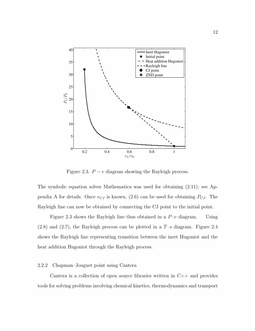
Figure 2.3. P − v diagram showing the Rayleigh process.

The symbolic equation solver Mathematica was used for obtaining (2.11); see Ap-

pendix A for details. Once vCJ is known, (2.6) can be used for obtaining PCJ . The

Rayleigh line can now be obtained by connecting the CJ point to the initial point.

Figure 2.3 shows the Rayleigh line thus obtained in a P–v diagram. Using

(2.8) and (2.7), the Rayleigh process can be plotted in a T–s diagram. Figure 2.4

shows the Rayleigh line representing transition between the inert Hugoniot and the

heat addition Hugoniot through the Rayleigh process.

2.2.2 Chapman–Jouguet point using Cantera

Cantera is a collection of open source libraries written in C++ and provides

tools for solving problems involving chemical kinetics, thermodynamics and transport

13

−1 0 1 2 3 4 5 60

2

4

6

8

10

12

14

∆s/R

T1/T

0

Inert Hugoniot

Initial point


Rayleigh line

CJ Point

ZND point

Figure 2.4. T–s diagram showing the Rayleigh process.

processes [22]. In this work, we use Cantera for obtaining solutions to the H2–O2

detonation problem. This allows us to take into account non-equilibrium effects by

including detailed chemistry and local thermodynamic equilibrium at each time and

location.

The properties of the CJ point obtained using the analytical solution devel-

oped in this section agree well with those computed using Cantera. Details of these

calculations can be found in Appendix C.

2.3 Obtaining the ZND point

The ZND point is the state attained by the gases after shock compression. It

is also called the von Neumann spike. We obtain the Mach number of the detona-

14

Figure 2.5. Flowchart describing the process of obtaining the CJ and ZND points.

tion wave for H2–O2 detonation from Cantera. By using normal shock relations, we

analytically obtain properties at the ZND point. The analytical results were verified

by Cantera. The P–v diagram in Fig. 2.3 and the T–s diagram in Fig. 2.4 depict the

ZND point.

2.4 Summary

In this chapter we derived the Rankine-Hugoniot relations. The heat addition

Hugoniot was used for obtaining the CJ point using the CJ detonation theory. The

15

ZND point was obtained based on the ZND theory of detonation. The methodology

to obtain the CJ and ZND points has been summarized in the flowchart 2.5. All

results agree well with those obtained from Cantera.

CHAPTER 3

ZND TO CJ TRANSITION

The transition from the ZND point to the CJ point occurs in the reaction zone

following the shock compression zone (see figure 1.3). In this chapter we analyze the

effect of friction on this transition for H2–O2 detonation.

3.1 ZND to CJ transition modeling using Cantera

Cantera includes libraries written in C++ that can be accessed using a Matlab

interface. We use Cantera for numerically solving the H2–O2 detonation problem with

detailed chemistry, assuming local chemical equilibrium. Refer to Appendix C for the

Matlab code used for accessing Cantera, written by Eric Braun (graduate student,

University of Texas at Arlington).

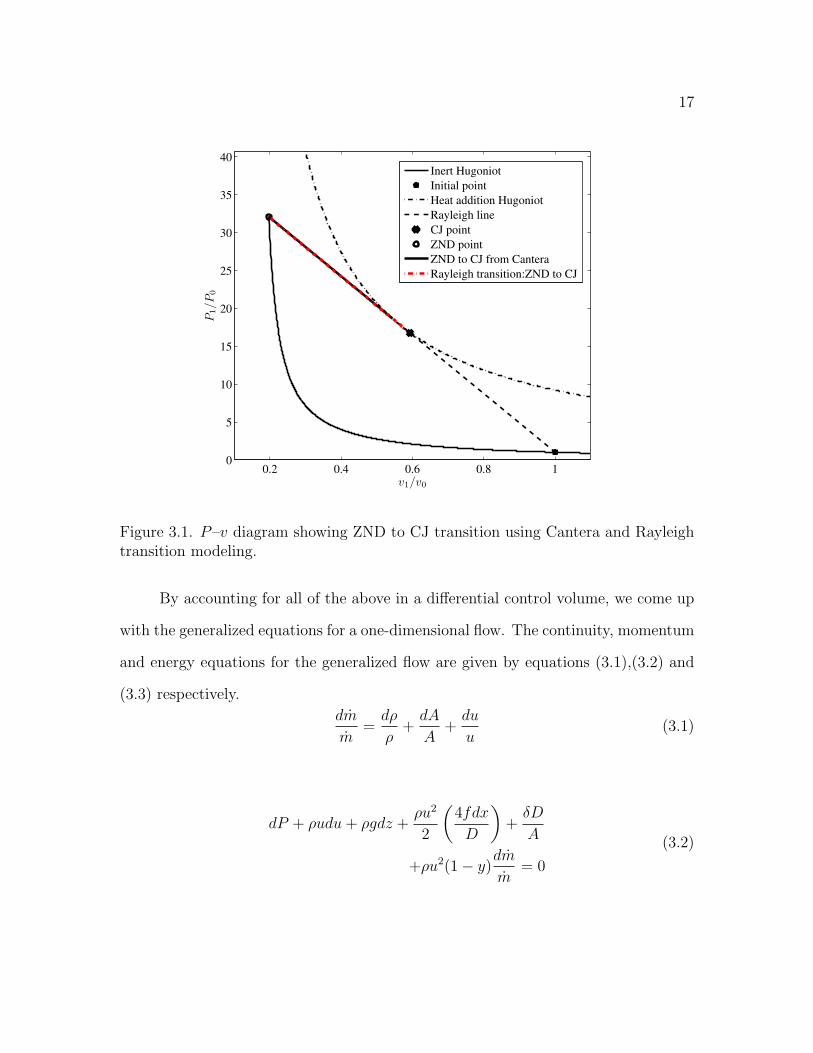
The path for ZND to CJ transition predicted using Cantera can be approxi-

mated well using a straight line in a P–v diagram. The slope of this line is identical

to a Rayleigh line originating from the CJ point. Figure 3.1 compares the path for

transition modeled using a Rayleigh line with that predicted using Cantera.

3.2 Generalized flow model

In the previous section, we modeled the ZND to CJ transition using Cantera,

which accounts for detailed chemistry. In real flows, however, there are many other

factors responsible for changes in flow properties, such as wall friction, change in

cross-sectional area, heat transfer through the walls, buoyancy effects, etc. [23].

16

17

0.2 0.4 0.6 0.8 10

5

10

15

20

25

30

35

40

v1/v0

P1/P

0

Inert Hugoniot

Initial point


Rayleigh line

CJ point

ZND point

ZND to CJ from Cantera

Rayleigh transition:ZND to CJ

Figure 3.1. P–v diagram showing ZND to CJ transition using Cantera and Rayleightransition modeling.

By accounting for all of the above in a differential control volume, we come up

with the generalized equations for a one-dimensional flow. The continuity, momentum

and energy equations for the generalized flow are given by equations (3.1),(3.2) and

(3.3) respectively.

dm

m=dρ

ρ+dA

A+du

u(3.1)

dP + ρudu+ ρgdz +ρu2

2

(4fdx

D

)+δD

A

+ρu2(1− y)dm

m= 0

(3.2)

18

Here 4f dx/D is the effect of wall friction and is termed as the friction factor.

δW − δQ+ (m+ dm)

[h+ dh+

u2

2+ d

(u2

2

)+ g(z + dz)

]−m

(h+

u2

2+ gz

)− dm

(hi +

u2i

2+ gzi

)= 0

(3.3)

Neglecting higher order terms, from equation (3.3) we obtain,

δW − δQ+ dh+ d

(u2

2

)+gdz

+

[(h+

u2

2+ gz

)−(hi +

u2i

2+ gzi

)]dm

m= 0

(3.4)

Here the subscript i denotes the properties of the fluid through a secondary inlet

(for example, a fuel injector). Also δW and δQ are the work done by the fluid and

heat transfer through the walls respectively. Using the definition of total enthalpy,

equation (3.4) can be written as

δW − δQ+ dH + dHi = 0 (3.5)

where the total enthalpy H = h+ u2/2 + gz, and dHi = (H −Hi)dm/m.

3.2.1 Generalized flow model: perfect gas

For a perfect gas, the generalized flow model can be written in terms of eight

distinct flow properties as given in (3.6) [24].

19

0 1 0 1 0 0 0 0

1 0γM2

2 0 γM2 0 0 0

1 −1 −1 0 0 0 0 0

0 0 12

−1 1 0 0 0

0 0 1 0(γ − 1)M2

ψ0 0 0

1 0 0 0γM2

ψ−1 0 0

−1 0 0 0 − 2γM2

1 + γM2 0 1 0

γ − 1γ 0 −1 0 0 0 0 1

·

dPPdρρ

dTTduu

dMMdPtPtdFFdsCp

=

dmm − dA

A

K + L

0

0

dTtTt

0

dAA

0

(3.6)

where

ψ = 1 +γ − 1

2M2

K = − γM2

2

(4fdx

D

)L = − γM2(1− y)

dm

m

Here the impulse function is defined as F = PA + mu. In this work, we use the

generalized equations for a perfect gas to include the effects of only heat addition and

friction.

3.3 Combined flow model: heat addition and friction

A combined flow model is proposed that would represent a flow with wall friction

and heat addition. By neglecting other effects, the system (3.6) can hence be written

as

20

0 1 0 1 0 0 0 0

1 0γM2

2 0 γM2 0 0 0

1 −1 −1 0 0 0 0 0

0 0 12

−1 1 0 0 0

0 0 1 0(γ − 1)M2

ψ0 0 0

1 0 0 0γM2

ψ−1 0 0

−1 0 0 0 − 2γM2

1 + γM2 0 1 0

γ − 1γ 0 −1 0 0 0 0 1

dPPdρρ

dTTduu

dMMdPtPtdFFdsCp

=

0

−γM2

2

(4fdxD

)0

0

dTtTt

0

0

0

(3.7)

(3.7) is of the form Ax = B, where matrix A is the matrix of coefficients and x is

a vector of property changes; x can be obtained by inverting A using Cramer’s rule.

An explicit equation for dM/M can hence be obtained:

dM

M=

(4fdx

D

)(γM2ψ

2(1−M2)

)+dTtTt

(1 + γM2)ψ

2(1−M2)(3.8)

Dividing by dx yields

dM

dx= M

[4f

D

γM2ψ

2(1−M2)+dTtdx

(1 + γM2)ψ

2Tt(1−M2)

](3.9)

(3.9) is a non-linear equation, and must be integrated numerically from MZND to

MCJ . Here, MZND is obtained from the analysis discussed in chapter 2, and MCJ ≡ 1.

This assumption is consistent with the CJ theory of detonation. The changes in the

seven remaining flow properties can be obtained by using the solution of (3.9) and

21

standard flow relations. We obtain the properties of pressure, specific volume, total

temperature and entropy by using the following equations:

PCJPZND

=mCJ

mZND

MZND

MCJ

TtCJ

(1 +

γ − 12 M2

ZND

)TtZND

(1 + γ−1

2M2

CJ

) (3.10a)

ρCJρZND

=PCJPZND

TZNDTCJ

(3.10b)

TCJTZND

=TtCJ

(1 +

γ − 12 M2

ZND

)TtZND

(1 +

γ − 12 M2

CJ

) (3.10c)

The change in entropy can be computed using the integrated Gibbs equation (2.7).

See the Matlab code in Appendix B for details.

3.4 Results and discussion

In the previous section a combined flow model was proposed, which takes into

account the effects of wall friction. The model provides us with a system of differential

equations for changes in the flow properties. In this section we analyze the results

obtained from the combined flow model for the transition from ZND to CJ point.

Numerically integrating (3.9), we obtain the Mach number variation in the

reaction zone as a function of distance from the leading shock. Using (3.10a), (3.10b),

(3.10c), (2.7) and the Mach number variation from the ZND to CJ points, we can plot

the changes in the P–v and T–s diagrams. Figures 3.2 and 3.3 show the variation in

properties using the combined flow model with different friction factors denoted by

4fdx/D. Here the Fanning friction factor f is varied from 1× 10−6 to 1× 10−2.

From figure 3.2, we see that the CJ point predicted using the combined flow

model occurs at a lower pressure when compared with the CJ point predicted using

inviscid analysis. Both, pressure and specific volume at the CJ point reduce as friction

22

0.1 0.2 0.3 0.4 0.5 0.6 0.7 0.8 0.9 1 1.10

5

10

15

20

25

30

35

40

v1/v0

P1/P

0

Inert Hugoniot

Initial point


Rayleigh line

CJ point

ZND point



Combined flow model with friction

Sub−CJ points

Figure 3.2. P–v diagram showing the transition between ZND to CJ point withcombined flow model including heat addition and friction.

at the walls increases. In the T–s diagram shown in figure 3.3, we observe that

increasing friction reduces the temperature at the CJ point. Figures 3.4 and 3.5

show the locus of all the CJ points for various friction factors. We observe that with

increase in friction factor the CJ point reduces. We also observe that the reduction

in the CJ points have a limiting value as the Fanning friction factor reaches 1× 10−2.

We obtain a family curves by varying the friction factor, each with its unique

CJ point. Hence we propose the existence of a family of Hugoniots corresponding to

different CJ points. Figures 3.6 and 3.7 show Hugoniots corresponding to two such

CJ points. We infer from the above observations that with increasing friction, the

23

−1 0 1 2 3 4 5 60

2

4

6

8

10

12

14

∆s/R

T1/T

0

Inert Hugoniot

Initial point


CJ Point

ZND point

Rayleigh transition


Sub−CJ points

Figure 3.3. T − s diagram showing the transition between ZND to CJ point withcombined flow model including heat addition and friction.

non-dimensional heat release α decreases. This implies that the maximum heat added

to the heat through combustion reduces.

3.5 Summary

In this chapter, we simplified the generalized one-dimensional flow for a perfect

gas to incorporate the effects of only friction, leading to the combined flow model.

Flow properties were computed by numerical integration from the ZND point to the

CJ point. We analyze the results to observe that the combined flow model gives

24

0.1 0.2 0.3 0.4 0.5 0.6 0.7 0.8 0.9 1 1.10

5

10

15

20

25

30

35

40

v1/v0

P1/P

0

Inert Hugoniot

Initial point


Rayleigh line

CJ point

ZND point




Sub−CJ points

Locus of CJ points

Figure 3.4. P–v diagram showing the transition between ZND to CJ point withcombined flow model including heat addition and friction.

us a family of transition curves for different friction factors, which lead to lower CJ

points. This concurs with experimental observations. We conclude that a lower CJ

point represents a lower α, i.e. heat of reaction. Hence distinct Hugoniot lines pass

through these CJ points.

25

−1 0 1 2 3 4 5 60

2

4

6

8

10

12

14

∆s/R

T1/T

0

Inert Hugoniot

Initial point


CJ Point

ZND point

Rayleigh transition


Sub−CJ points

Locus of CJ points

Figure 3.5. T − s diagram showing the transition between ZND to CJ point withcombined flow model including heat addition and friction.

26

0.1 0.2 0.3 0.4 0.5 0.6 0.7 0.8 0.9 1 1.10

5

10

15

20

25

30

35

40

v1/v0

P1/P

0

Inert Hugoniot

Initial point


Rayleigh line

CJ point

ZND point




Sub−CJ points

Unique Hugoniots

Figure 3.6. P–v diagram showing distinct Hugoniots for arbitrary values of the frictionfactor.

27

−1 0 1 2 3 4 5 60

2

4

6

8

10

12

14

∆s/R

T1/T

0

Inert Hugoniot

Initial point


CJ Point

ZND point

Rayleigh transition


Sub−CJ points

Unique Hugoniots

Figure 3.7. T–s diagram showing distinct Hugoniots for arbitrary values of the frictionfactor.

CHAPTER 4

SUMMARY AND CONCLUSIONS

In chapter 1, we discussed the two established theories of detonation, i.e., the

CJ and ZND theories. The CJ theory postulates the existence of a thin reaction zone

that travels with the shock. As a result, the transition from the inert Hugoniot to the

heat addition Hugoniot can be represented by a Rayleigh line. The Rayleigh line is

tangent to the heat addition Hugoniot at the CJ point, which is the point of chemical

equilibrium. At the CJ point, the Mach number of the burnt gases is unity in the

frame of reference of the detonation wave. This theory, however, fails to account for

the non-equilibrium chemistry and an experimentally observed pressure peak, known

as the von Neumann spike (also called the ZND point). The ZND theory, on the other

hand, postulates the existence of separate shock compression and reaction zones. This

allows it to account for the pressure rise at the ZND point. After the ZND point,

there are chemical reactions that occur in the reaction zone, and chemical equilibrium

is attained at the CJ point. The ZND theory, although a better detonation model,

fails to map the transition from the ZND point to the CJ point. In this work, an

analytical model has been developed for H2–O2 detonation, allowing us to map this

transition by including detailed chemistry, and the effect of friction.

In chapter 2, the ZND to CJ transition is obtained numerically using Cantera,

which takes the non-equilibrium effects of the reacting gases into account. We showed

that this transition can be approximated well by a Rayleigh line.

In chapter 3, a combined flow transition model was constructed incorporating

the effects of wall friction (relevant to the shock tube experimental conditions). With

28

29

different values of friction factors we obtain a unique curve ending in a unique CJ

point. These CJ points agree with the initial premise of a sub-CJ condition found

experimentally. We observe from the model that the heat addition Hugoniots passing

though these uniques CJ points have a lower heat of reaction α. This leads us to

conclude that the family of CJ points have unique Hugoniots passing through them,

indicative of their respective heat of reaction α. This implies that an increase in wall

friction leads to lower heat addition, since the flow becomes sonic faster. We also

observe a reduction in maximum temperature with increase in wall friction.

In conclusion, we see that the analytical model qualitatively agrees with the

experimental results, by predicting a sub-CJ state of equilibrium .

4.1 Future work

In the current work, we focus on H2-O2 detonation chemistry leading to a model

based on the Rayleigh line of heat addition, which is specific to these reactants. An

analysis of a larger number of detonation chemistries would allow us to construct

a more generalized detonation model. The only input parameters for such a model

would be the heat of reaction α and the non-dimensional friction factor 4f dx/D. A

detailed analytical model to take into account the effect of friction on the flow behind

the detonation wave can be incorporated so as to capture the effects of boundary layer

growth, similar to Mirel’s problem. A future study could also undertake numerical

modeling of the effects of friction.

APPENDIX A

MATHEMATICA: SOLUTION FOR THE CJ POINT

30

31

p2 = p1 ∗ (gam + 1− (gam− 1) ∗ v2/v1 + 2 ∗ (gam− 1) ∗ alpha)/p2 = p1 ∗ (gam + 1− (gam− 1) ∗ v2/v1 + 2 ∗ (gam− 1) ∗ alpha)/p2 = p1 ∗ (gam + 1− (gam− 1) ∗ v2/v1 + 2 ∗ (gam− 1) ∗ alpha)/

((gam + 1) ∗ v2/v1− gam + 1)((gam + 1) ∗ v2/v1− gam + 1)((gam + 1) ∗ v2/v1− gam + 1)

p1(1+2alpha(−1+gam)+gam− (−1+gam)v2v1 )

1−gam+(1+gam)v2

v1

dpdv = p1/v1 ∗ (−(gam− 1) ∗ ((gam + 1) ∗ v2/v1− (gam− 1))dpdv = p1/v1 ∗ (−(gam− 1) ∗ ((gam + 1) ∗ v2/v1− (gam− 1))dpdv = p1/v1 ∗ (−(gam− 1) ∗ ((gam + 1) ∗ v2/v1− (gam− 1))

−((gam + 1)− (gam− 1) ∗ v2/v1 + 2 ∗ alpha ∗ (gam− 1)) ∗ (gam + 1))/−((gam + 1)− (gam− 1) ∗ v2/v1 + 2 ∗ alpha ∗ (gam− 1)) ∗ (gam + 1))/−((gam + 1)− (gam− 1) ∗ v2/v1 + 2 ∗ alpha ∗ (gam− 1)) ∗ (gam + 1))/

((gam + 1) ∗ v2/v1− gam + 1)∧2((gam + 1) ∗ v2/v1− gam + 1)∧2((gam + 1) ∗ v2/v1− gam + 1)∧2

p1(−(1+gam)(1+2alpha(−1+gam)+gam− (−1+gam)v2v1 )+(1−gam)(1−gam+

(1+gam)v2v1 ))

v1(1−gam+(1+gam)v2

v1 )2

Together[Solve[dpdv==(p2− p1)/(v2− v1), v2]]Together[Solve[dpdv==(p2− p1)/(v2− v1), v2]]Together[Solve[dpdv==(p2− p1)/(v2− v1), v2]]{v2→ −alphav1+gamv1+gam2v1+alphagam2v1−

√alpha(−1+gam2)(−alpha+2gam+alphagam2)v12

gam(1+gam)

},{

v2→ −alphav1+gamv1+gam2v1+alphagam2v1+√

alpha(−1+gam2)(−alpha+2gam+alphagam2)v12

gam(1+gam)

}

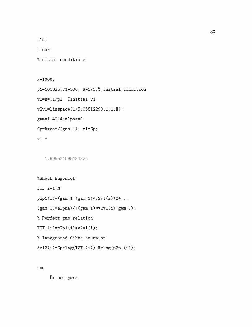
APPENDIX B

MATLAB CODE

32

33

clc;

clear;

%Initial conditions

N=1000;

p1=101325;T1=300; R=573;% Initial condition

v1=R*T1/p1 %Initial v1

v2v1=linspace(1/5.06812290,1.1,N);

gam=1.4014;alpha=0;

Cp=R*gam/(gam-1); s1=Cp;

v1 =

1.696521095484826

%Shock hugoniot

for i=1:N

p2p1(i)=(gam+1-(gam-1)*v2v1(i)+2*...

(gam-1)*alpha)/((gam+1)*v2v1(i)-gam+1);

% Perfect gas relation

T2T1(i)=p2p1(i)*v2v1(i);

% Integrated Gibbs equation

ds12(i)=Cp*log(T2T1(i))-R*log(p2p1(i));

end

Burned gases

34

gam1=1.205666499829051;

R1=692;

%Hugoniot with heat addition

v3v1=linspace(0.3,1.1,N);

H1=4.47e3;U1=0;H2=2.853e6;U2=2.835e3;

Cp1=R1*gam1/(gam1-1);

alpha=((H2+U2^2/2)-(H1+U1^2/2))/(p1*v1)

for i=1:N

p3p1(i)=(gam1+1-(gam1-1)*v3v1(i)+2*...

(gam1-1)*alpha)/((gam1+1)*v3v1(i)-gam1+1);

T3T1(i)=p3p1(i)*v3v1(i);%*R/R1;


end

alpha =

39.948472949389178

Hugo heat

%Hugoniot with heat addition


U7=1.8e3;

alpha7=((H2+U7^2/2)-(H1+U1^2/2))/(p1*v1)

for i=1:N

p7p1(i)=(gam1+1-(gam1-1)*v7v1(i)+2*...

(gam1-1)*alpha7)/((gam1+1)*v7v1(i)-gam1+1);

35

T7T1(i)=p7p1(i)*v7v1(i);%*R/R1;


end


U8=0.9e3;

alpha8=((H2+U8^2/2)-(H1+U1^2/2))/(p1*v1)

for i=1:N

p8p1(i)=(gam1+1-(gam1-1)*v8v1(i)+2*...

(gam1-1)*alpha8)/((gam1+1)*v8v1(i)-gam1+1);

T8T1(i)=p8p1(i)*v8v1(i);%*R/R1;


end

alpha7 =

25.994938917975567

alpha8 =

18.926876090750437

%Rayleigh line

N=1000;

MZND=5.255;

M2=linspace(0.4114,0.9662364,N);

for i=1:N

36

p4p1(i)=(1+gam*MZND^2)/(1+gam*M2(i)^2);

v4v1(i)=1/(((1+gam*M2(i)^2)/(1+gam*MZND^2))*(MZND/M2(i))^2);

T4T1(i)=p4p1(i)*v4v1(i);%*R/R1;


prayp1(i)=1+gam*MZND^2-v3v1(i)*MZND*gam;

end

ZND point

vzndv1=1/5.06812290; pzndp1=32.0637928;

TzndT1=pzndp1*vzndv1;

ds1znd=Cp*log(TzndT1)-R*log(pzndp1);

CJ point

vcjv1=(gam1-alpha+gam1^2*(1+alpha)-(alpha*(gam1^2-1)*...

(2*gam1-alpha+alpha*gam1^2))^0.5)/(gam1*(gam1+1));

pcjp1=(gam1+1-(gam1-1)*vcjv1+2*...

(gam1-1)*alpha)/((gam1+1)*vcjv1-gam1+1);

TcjT1=pcjp1*vcjv1;%*R/R1;

ds1cj=Cp*log(TcjT1)-R*log(pcjp1);

%Importing Data from cantera for T-S diagram

% Tdata = xlsread(’T-s.xls’,1,’B8:B232’);

% Sdata = xlsread(’T-s.xls’,1,’F8:F232’);

% Tdata1=Tdata/T1;

% Sdata1=Sdata/Cp;

37

Friction

Initialize

D=0.25;

p1=101325;T1=300; R=573;

v1=R*T1/p1; %Initial v1

gam=1.4014; M0=0.41223200;

v0=1/5.06812290*v1; p0=32.0637928*101325;

t0=p0*v0/R; T0=t0*(1+(gam-1)/2*M0^2);

P0=p0*(1+(gam-1)/2*M0^2)^(gam/(gam-1));

% Use previous value of alpha

xmin=0; %xmax=12;

dx0=1e-01;

Combined flow model:While loop

tic

f0=0.000001;

E=10; fmax=0.01;

ff=linspace((f0+fmax)/10,fmax,7);

frc(1:3)=[f0, 100*f0, (f0+fmax)/20];

frc(4:10)=ff;

for e=1:E

i=1; Mcomp=M0;

while (Mcomp<0.99)

if (Mcomp<0.9)

dx=dx0;

38

elseif (Mcomp<0.95)

dx=dx0/5;

else

dx=dx0/20;

end

if (mod(i,10000)==0)

Mcomp,i

end

if (i==1)

M(i)=M0;

T(i)=T0;

p(i)=p0;

x(i)=xmin;

else

Mx=M(i-1);

Tx=T(i-1);

px=p(i-1);

psi=1+(gam-1)/2*Mx^2;

dTdx=alpha*dx;

dMdx=Mx*(4*frc(e)/D*gam*Mx^2*psi/2/(1-Mx^2)+.....

dTdx/Tx*(1+gam*Mx^2)*psi/2/(1-Mx^2));

M(i)=Mx+dx*dMdx;

T(i)=Tx+dx*dTdx;

p(i)=px*Mx/M(i)*(T(i)*psi/Tx/(1+(gam-1)/2*M(i)^2))^0.5;

x(i)=x(i-1)+dx;

end

39

t(i)=T(i)/(1+(gam-1)/2*M(i)^2);

P(i)=p(i)*(1+(gam-1)/2*M(i)^2)^(gam/(gam-1));

v(i)=R*t(i)/p(i);

Mcomp=M(i);

dsfr(i)=Cp*log(t(i)/T1)-R*log(p(i)/p1); % addition

i=i+1;

end

str_n(e)=i-1;

str_t(e,:)=t;

str_ds(e,:)=dsfr;

str_p(e,:)=p;

str_v(e,:)=v;

end

toc

Mcomp =

0.979756542138573

i =

10000

Elapsed time is 3.320929 seconds.

40

Plots Pv

figure(1)

plot(v2v1,p2p1,’k-’,’linewidth’,2); hold on;

plot(1,1,’k*’,’linewidth’,6);

plot(v3v1,p3p1,’k-.’,’linewidth’,2);

plot([1,vcjv1],[1,pcjp1],’k--’,’linewidth’,2)

plot (0.593,16.71,’kx’,’linewidth’,10) % CJ point

plot(1/5.06812290,32.0637928,’ko’,’linewidth’,3)

plot([1/5.06812290,1/1.8384],[32.0637928,18.653],’k-’,’linewidth’,3)

plot(v4v1,p4p1,’r-.’,’linewidth’,3);

for e=1:E

pp=plot(str_v(e,1:str_n(e))/v1,str_p(e,1:str_n(e))/p1);

if (e~=1)

’LegendInformation’),’IconDisplayStyle’,’off’)

end

end

hold off;

axis([0.1 max(v2v1) 0 max(p3p1)])

set(gca,’FontSize’,15)

set(gca,’FontName’,’Times’)

xlabel(’$v_1/v_0$’,’FontSize’,15,’FontName’,’Times’, ...

’Interpreter’, ’latex’)

ylabel(’$P_1/P_0$’,’FontSize’,15,’FontName’,’Times’, ...

’Interpreter’, ’latex’)

legend(’Inert Hugoniot’,’Initial point’, ...

’Heat addition Hugoniot’,’Rayleigh line’,...

41

’CJ point’,’ZND point’,’ZND to CJ from Cantera’, ...

’Rayleigh transition:ZND to CJ’...

,’Combined flow model with friction’,’Unique Hugoniot’)

hold off

Plot TS

figure(2)

plot(ds12/R,T2T1,’k-’,’linewidth’,2);hold on;%ds14,T4T1,’b:’ inert

plot(0,1,’k*’,’linewidth’,6)%initial point

plot(ds13/R,T3T1,’k-.’,’linewidth’,2); % Heat addition

plot(ds1cj/R,TcjT1,’kx’,’linewidth’,10); % CJ point

plot(ds1znd/R,TzndT1,’ko’,’linewidth’,3); % ZND point

plot(ds14/R,T4T1,’b--’,’linewidth’,2)% Transition

for e=1:E

tt=plot((str_ds(e,1:str_n(e)))/R,str_t(e,1:str_n(e))/T1);

if (e~=1)

set(get(get(tt,’Annotation’),’LegendInformation’)...

,’IconDisplayStyle’,’off’)

end

end

plot(ds17/R,T7T1,’b-.’,’linewidth’,2)

plot(ds18/R,T8T1,’b-.’,’linewidth’,2)

hold off;

set(gca,’FontSize’,15)

set(gca,’FontName’,’Times’)

42

xlabel(’$\Delta s/R$’,’FontSize’,15,’FontName’,’Times’, ...

’Interpreter’,’latex’)

ylabel(’$T_1/T_0$’,’FontSize’,15,’FontName’,’Times’, ...

’Interpreter’,’latex’)

legend(’Inert Hugoniot’,’Initial point’,’Heat addition Hugoniot’,...

’CJ Point’,’ZND point’,’Rayleigh transition’,....

’Combined flow model with friction’,’Unique Hugoniots’)

APPENDIX C

CANTERA CODE FOR H2-O2 SIMULATION

43

44

%This program solves for the post-detonation wave variables

%using a ZND model.

%This should then be placed into the RDWE code and iterated.

clear;clc; %remove when placed in a larger program

%Initial mixture states for the detonation wave

P1 = 101325;

T1 = 300;

q = ’H2:2 O2:1’;

mech = ’h2o2_highT.cti’;

%Premix speed of sound (change m if not stoichiometric H2-air!)

gas = GRI30;

set(gas, ’Temperature’, T1, ’Pressure’, P1, ’MoleFractions’, ...

’H2:2,O2:1’);

T_1 = temperature(gas); %Temperature, K

P_1 = pressure(gas); %Pressure, Pa

rho_1 = density(gas); %Density, kg/m^3

S_1 = entropy_mass(gas); %Entropy, J/(kg K)

X_1 = moleFractions(gas); %Post-detonation mole fractions

h_1 = enthalpy_mass(gas); %Enthalpy, J/(kg K)

a_1 = soundspeed(gas); %Post-detonation SOS, m/s

cp_1 = cp_mass(gas); %cp, J/(kg K)

cv_1 = cv_mass(gas); %cv, J/(kg K)

m_1 = meanMolecularWeight(gas); %Molecular weight

45

gamma_1 = cp_1/cv_1; %Specific heat ratio

R_1 = 8314.472/m_1; %Gas constant, kJ/(kg K)

%Use Cal-Tech SD Toolbox programs to calculate ZND solution

[cj_speed,gas2] = znd_CJ(1, P1, T1, q, mech, ’h2o2’, 2);

%Recall properties of the post-ZND gas mixture

T_ZND = temperature(gas2); %Temperature, K

P_ZND = pressure(gas2); %Pressure, Pa

rho_ZND = density(gas2); %Density, kg/m^3

S_ZND = entropy_mass(gas2); %Entropy, J/(kg K)

V_ZND = cj_speed; %Propagation speed, m/s

X_ZND = moleFractions(gas2); %Post-detonation mole fractions

h_ZND = enthalpy_mass(gas2); %Enthalpy, J/(kg K)

a_ZND = soundspeed(gas2); %Post-detonation SOS, m/s

cp_ZND = cp_mass(gas2); %cp, J/(kg K)

cv_ZND = cv_mass(gas2); %cv, J/(kg K)

m_ZND = meanMolecularWeight(gas2); %Molecular weight

%Calculate additional properties after the wave

gamma_ZND = cp_ZND/cv_ZND; %Specific heat ratio

R_ZND = 8314.472/m_ZND; %Gas constant, kJ/(kg K)

M_ZND = V_ZND/a_1; %Detonation Mach number

REFERENCES

[1] P. A. Thompson, Compressible Fluid Dynamics. McGraw-Hill, 1972.

[2] M. D. Salas, “The curious events leading to the theory of shock waves,” Shock

waves, vol. 16, p. 477487, 2007.

[3] K. K. Kuo, Principles of Combustion. John Wiley and Sons, 1986, ch. 4.1.

[4] W. Fickett and W. C. Davis, Detonation Theory and Experiment. Dover Pub-

lications Inc, 2000, ch. 1.

[5] A. H. Shapiro, The Dynamics and Thermodynamics of Compressible Fluid Flow.

Ronald Press, 1953, vol. 1.

[6] D. L. Chapman, “Rate of explosion in gases,” Philos Mag, vol. 14, pp. 1091–1094,

1899.

[7] J. Jouguet, “Propagation of chemical reactions in gases,” J.de Mathematiques

Pures et Appliquees, vol. 1, p. 347425, 1905.

[8] Y. B. Zeldovich, “Theory of the propagation of detonation in gaseous systems,”

Zhurnal Experimentalnoi i Teoreticheskoi Fizik, vol. 10, p. 542568, 1940, available

in translation as NACA TM-1261.

[9] Y. B. Zeldovich and A. S. Kompaneets, Theory of Detonation. Academic Press,

NY, 1960, ch. 4.1, english translation of original Russian.

[10] Y. B. Zeldovich and Y. P. Raizer, Physics of Shock Waves and High-Temperature

Hydrodynamic Phenomena. Wiley, NY, 1966, vol. 1 and 2, ch. 10.

[11] J. von Neumann, Theory of detonation waves-John von Neumann, Collected

Works. Macmillan, 1942.

46

47

[12] W. Doring, “Detonation processes in gases,” Ann. Phys, vol. 43, p. 421436, 1943,

available in translation as NACA TM-1261.

[13] J. Z. S. Browne and J. E. Shepherd, “Numerical solution methods for

shock and detonation jump conditions,” Aeronautics and Mechanical Engi-

neering California Institute of Technology Pasadena, CA USA 91125, Tech.

Rep. FM2006.006 http://www.galcit.caltech.edu/EDL/public/cantera/doc/tex/

ShockDetonation/ShockDetonation.pdf.

[14] J. N. Johnson and R. Cheret, “Classic papers in shock compression science,”

Springer, 1998.

[15] A. N. Dremin, Towards detonation Theory. Springer, 1999, ch. 2.2.

[16] R. Petela, “Application of exergy analysis to the hydrodynamic theory of det-

onation in gases,” Fuel Processing Technology, vol. 67, no. 2, pp. 131 – 145,

2000.

[17] J. Kentfield, “Thermodynamics of airbreathing pulse-detonation engines,” Jour-

nal of Propulsion and Power, vol. 18, no. 6, pp. 1170–1175, 2002.

[18] W. H. Heiser and D. T. Pratt, “Thermodynamic cycle analysis of pulse deto-

nation engines,” Journal of Propulsion and Power, vol. 18, no. 1, pp. 68–76,

2002.

[19] H. Mirels and J. F. Mullen, “Small perturbation theory for shock-tube attenua-

tion and nonuniformity,” Physics of Fluids, vol. 7, no. 8, pp. 1208–1218, 1964.

[20] I. Glass and J. P. Sislian, Nonstationary flows and shock waves. Oxford Uni-

versity Press, 1994.

[21] F. J. Zeleznik and S. Gordon, “A general i b m 704 or 7090 computer pro-

gram for computation of chemical equilibrium compositions, rocket performance

and chapman-jouguet detonations,” NASA, Tech. Rep. Technical Note TN-1454,

1962.

48

[22] D. G. Goodwin, “Cantera user’s guide,” Division of Engineering and Applied

Science ,California Institute of Technology, Pasadena, CA USA, Tech. Rep., 2001.

[23] M. J.Zucrow and J. D. Hoffman, Gas dynamics multidimentional Flow. John

Wiley and sons, 1976, vol. 1, ch. 9.

[24] B. Hodge and K. Koenig, Compressible Fluid Dynamics with Personal Computer

Applications. Prentice-Hall, 1995.

BIOGRAPHICAL STATEMENT

Sushma Rao was born in Bangalore, India on January 15, 1982, to Sudha and

Sudheendra Rao. She was raised in the cosmopolitan suburb of Vashi, Navi Mumbai.

Sushma received a B.Arch. degree in Architecture from the University of Mumbai,

in 2004. During her career as an Architect, Sushma was involved in designing multi-

storied buildings as well as interiors for corporate offices. After working for three and

a half years as an Architect, she joined the University of Texas at Arlington (UTA)

for a Masters in Aerospace Engineering.

At UTA, Sushma’s interests were mainly in fluids and controls, although she

also enjoyed the odd course in Automobile Engineering. She decided to work in the

area of pulse detonation engines for her thesis with Prof. Frank Lu. During the last

semester of her Masters, Sushma worked as an intern at the Center for Space Nuclear

Research at Idaho National Laboratories, Idaho, USA. Her work involved feasibility

studies of a sample return mission from Mars.

During her graduate studies, Sushma married her long time boyfriend Pratik

Donde.

Sushma’s interest outside academia include hiking and other adventure sports.

She has trekked various peaks in the Himalayas and Western Ghats in India, and also

in the Rocky Mountains of Idaho, USA.

49

Documents

EFFECT OF FRICTION ON THE ZEL’DOVICH{VON …