Embed Size (px)
Citation preview

EFFECT OF FRAME SHAPE AND GEOMETRY ON THE GLOBAL
BEHAVIOR OF RIGID AND HYBRID FRAME UNDER
EARTHQUAKE EXCITATIONS
by
S. M. ASHFAQUL HOQ
Presented to the Faculty of the Graduate School of
The University of Texas at Arlington in Partial Fulfillment
of the Requirements
for the Degree of
MASTER OF SCIENCE IN CIVIL ENGINEERING
THE UNIVERSITY OF TEXAS AT ARLINGTON
May 2010

Copyright © by S. M. Ashfaqul Hoq 2010
All Rights Reserved

iii
ACKNOWLEDGEMENTS
I would like to express my sincere gratitude to my thesis advisor, Dr. Ali
Abolmaali, for his continuous help and guidance in the accomplishment of this work. I
really appreciate Dr. Ali Abolmaali for his unrestricted personal guidance throughout this
study, for bringing out the best of my ability. His kind supervision, encouragement,
assistance and invaluable suggestion at all stages of the work made it possible to
complete this work. The services he offered personally were a great help.
I would like to express my sincere thanks to Dr. John H. Matthys and Dr.
Guillermo Ramirez, for their time to serve on my thesis committee and providing
invaluable suggestions and advice.
I would like to thank Dr. Tri Le, Dobrinka Radulova, Mohammad Razavi and all
my colleagues and friends for their moral support and helpful discussions.
Finally, I would like to express my heartfelt thanks to my parents and siblings for
their unconditional love, support, encouragement and blessings to complete my masters
program.
April 15, 2010

iv
ABSTRACT
EFFECT OF FRAME SHAPE AND GEOMETRY ON THE GLOBAL
BEHAVIOR OF RIGID AND HYBRID FRAME UNDER
EARTHQUAKE EXCITATIONS
S.M.Ashfaqul Hoq, M.S.
The University of Texas at Arlington, 2010
Supervising Professor: Dr. Ali Abolmaali
The primary focus of this study is to present a shape which will improve building
performance in earthquake excitations. The investigation started with a 3-, 9-, 12- and 20-
story rectangular frame. The seismic performance is observed for different earthquake
data with different frequency content. Then, the Rhombus Shape is introduced to
compare with the Rectangular Shape frames, keeping the height-to-width ratio and
loading the same. For the first part of the investigation, deflection and member forces are
compared between rhombus and rectangular shape considering all connections rigid. In
the second part of the study partially restrained connections are introduced in mid levels
of the high rise frames to observe the redistribution pattern of internal forces. The results
show that with all rigid connections, a rhombus shape performs better than a rectangular
frame in most of the cases. Also, partially restrained connections which forms hybrid
frame have more significant effects on the rectangular frame than the rhombus frame.

v
TABLE OF CONTENTS
ACKNOWLEDGEMENTS ............................................................................................... iii
ABSTRACT ....................................................................................................................... iv
LIST OF ILLUSTRATIONS ............................................................................................. ix
LIST OF TABLES ............................................................................................................ xii
Chapter Page
1. INTRODUCTION .................................................................................................1
1.1 Introduction .................................................................................................1
1.2 Background .................................................................................................6
1.2.1 Moment Frames (MFs) ........................................................................6
1.2.2 Concentrically Braced Frames (CBFs) ................................................8
1.2.3 Eccentrically Braced Frames (EBFs) .................................................10
1.3 Literature review .......................................................................................11
1.4 Objective of the Present Study ..................................................................16
1.5 Scope of the Study ....................................................................................16
1.7 Organization of the Present Study ............................................................17
2. BACKGROUND ON FRAME ANALYSIS .......................................................18
2.1 Introduction ..............................................................................................18
2.2 Analysis Methods.....................................................................................18

vi
2.2.1 Elastic Analysis Methods ..............................................................19
2.2.2 Inelastic Analysis Methods ..........................................................20
2.3 First Order Elastic Analysis .....................................................................20
2.4 Second Order Elastic Analysis.................................................................21
2.5 Inelastic Analysis .....................................................................................23
2.6 Dynamic Analysis of frame .....................................................................25
2.7 Modal Analysis ........................................................................................27
2.8 Step-by-Step Integration ..........................................................................28
2.8.1 Newmark’s Method .....................................................................29
2.8.1.1 Average Acceleration Method ..........................................30
2.8.1.2 Linear Acceleration Method .............................................31
2.8.2 Wilson θ Method ..........................................................................32
2.8.3 Hilber-Hughes-Taylor Method ....................................................33
3. EFFECT OF FRAME SHAPE AND GEOMETRY ON SEISMIC PERFORMANCE ........................................................................34
3.1 Introduction ..............................................................................................34
3.2 Three Story Frame ...................................................................................36
3.3 Nine Story Frame .....................................................................................38
3.4 Twelve Story Frame .................................................................................41
3.5 Twenty Story Frame ................................................................................43
3.6 Eathquake in consideration ......................................................................46
3.6.1 Generated Earthquake ..................................................................47

vii
3.6.2 ElCentro .......................................................................................51
3.6.3 Northridge ....................................................................................53
3.6.4 Parkfield .......................................................................................55
3.6.5 Kocaeli .........................................................................................57
3.7 Discussion of the Results .........................................................................61
4. HYBRID FRAME SYSTEMS ...........................................................................67
4.1 Introduction ..............................................................................................67
4.2 Semi-rigid Connection .............................................................................69
4.2.1 Moment-Rotation models ............................................................70
4.2.2 Bi-linear semi-rigid Connection Properties .................................72
4.3 Two-Story Test Frame .............................................................................73
4.4 20-Story Rectangular Hybrid Frame ........................................................76
4.5 20-Story Rhombus Hybrid Frame ............................................................79
4.6 Discussion of the Results .........................................................................82
5. CONCLUSIONS AND RECOMMENDATIONS .............................................92
5.1 Summary ..................................................................................................92
5.2 Conclusions ..............................................................................................93
5.3 Recommendations ....................................................................................95

viii
APPENDIX
A. TOP LATERAL DISPLACEMENT .........................................................96
B. AXIAL FORCES IN THE FRAME ELEMENTS ..................................112
C. SHEAR FORCES IN THE FRAME ELEMENTS ..................................153
D. BENDING MOMENTS IN THE FRAME ELEMENTS ........................194
E. MAXIMUM LATERAL DISPLACEMENT PROFILE .........................235
F. LATERAL INTER STORY DRIFT ........................................................251
G. LOAD CALCULATION .........................................................................267
REFERENCES ................................................................................................................270
BIOGRAPHICAL INFORMATION ...............................................................................276

ix
LIST OF ILLUSTRATIONS
Figure Page
1.1 20-Story Rectangular frame and equivalent Rhombus shape ........................................4
1.2 Typical CBF configurations ...........................................................................................9
1.3 Typical EBF configurations .........................................................................................11
2.1 Generalised Load-Displacement curve for different types of analysis ........................21
2.2 P-δ and P-Δ effects.......................................................................................................22
2.3 Average acceleration ....................................................................................................30
2.4 Linear acceleration .......................................................................................................31
2.5 Linear variation of acceleration over extended time steps ...........................................32
3.1 Three-Story Rectangular and Rhombus frame ............................................................37
3.2 First two Mode Shapes for 3-Story Rectangular Frame (a) Mode 1, (b) Mode 2 ................................................................................................37
3.3 First two Mode Shapes for 3-Story Rhombus Frame (a) Mode 1, (b) Mode 2 ................................................................................................37
3.4 Nine-Story Rectangular and Rhombus frame ..............................................................39
3.5 First two Mode Shapes for 9-Story Rectangular Frame (a) Mode 1, (b) Mode 2 ................................................................................................39
3.6 First two Mode Shapes for 9-Story Rhombus Frame (a) Mode 1, (b) Mode 2 ................................................................................................40
3.7 Twelve-Story Rectangular and Rhombus frame ..........................................................41
3.8 First two Mode Shapes for 12-Story Rectangular Frame (a) Mode 1, (b) Mode 2 ................................................................................................42

x
3.9 First two Mode Shapes for 12-Story Rhombus Frame (a) Mode 1, (b) Mode 2 ................................................................................................42
3.10 Twenty-Story Rectangular and Rhombus frames ......................................................44
3.11 First two Mode Shapes for 20-Story Rectangular Frame (a) Mode 1, (b) Mode 2 ..............................................................................................45
3.12 First two Mode Shapes for 20-Story Rhombus Frame (a) Mode 1, (b) Mode 2 ..............................................................................................45
3.13 Acceleration Time History of Generated Earthquake ................................................48
3.14 Fourier Spectrum of Generated Earthquake ..............................................................49
3.15 20S-289_100_2.89-TDux(RMR,RCR)-generated data .............................................50
3.16 Acceleration Time History of El Centro Earthquake .................................................52
3.17 Fourier Spectrum of El Centro Earthquake ...............................................................52
3.18 Acceleration Time History of Northridge Earthquake ...............................................54
3.19 Fourier Spectrum of Northridge Earthquake .............................................................54
3.20 Acceleration Time History of Parkfield Earthquake .................................................56
3.21 Fourier Spectrum of Parkfield Earthquake ................................................................56
3.22 Acceleration Time History of Kocaeli[Afyon Bay,N(ERD)] Earthquake .................58
3.23 Fourier Spectrum of Kocaeli[Afyon Bay,N(ERD)] Earthquake ................................58
3.24 Acceleration Time History of Kocaeli[Aydin,S(ERD)] Earthquake .........................59
3.25 Fourier Spectrum of Kocaeli[Aydin,S(ERD)] Earthquake ........................................60
4.1 Rotational deformation of a connection due to flexure ...............................................70
4.2 Typical moment-rotation curves ..................................................................................71
4.3 Semi-rigid element of a Hybrid frame .........................................................................71
4.4 Bi-linear moment-rotation curve ..................................................................................72

xi
4.5 Two story one bay test frame .......................................................................................74
4.6 Moment-Rotation relation used in previous study (Bhatti and Hingtgen,1995) ..........75
4.7 Hybrid Rectangular: 20S – 289_100_2.89 – (RCSR) – E(7-11) .................................78
4.8 Hybrid Rhombus: 20S – 289_100_2.89 – (RMSR) – E(7-11) ....................................80
4.9 Fat Hybrid Rhombus: 20S – 289_300_0.963 – (RMSR) – E(7-11) ............................81
4.10 Maximum lateral sway 20S-289_100_2.89–MDUx (RCR,RCSR)–E1m(7-11) .......82
4.11 20S – 289_100_2.89–LDr (RCR,RCSR) –E1m(7-11) ..............................................84
4.12 20S – 289_100_2.89 – BM (RCSR/RCR) – E1m(7-11) for Beams ..........................85
4.13 Maximum lateral sway 20S-289_100_2.89-MDUx(RMR,RMSR)-E1m(7-11) ........88
4.14 20S –289_100_2.89–LDr (RMR,RMSR)–E1m(7-11) ..............................................88
4.15 20S – 289_100_2.89 – BM (RMSR/RMR) – E1m(7-11) for Beams ........................89
xii
LIST OF TABLES
Table Page
3.1 Modal period and frequencies for 3-Story Frames (SAP 2000) ..................................38
3.2 Modal period and frequencies for 9-Story Frames (SAP 2000) ..................................40
3.3 Modal period and frequencies for 12-Story Frames (SAP 2000) ................................43
3.4 Modal period and frequencies for 20-Story Frames (SAP 2000) ................................46
3.5 Frequency Content for El Centro Earthquake ..............................................................53
3.6 Frequency Content for Northridge Earthquake ............................................................55
3.7 Frequency Content for Parkfield Earthquake ..............................................................57
3.8 Frequency Content for Kocaeli[Afyon Bay,N(ERD)] Earthquake ..............................59
3.9 Frequency Content for Kocaeli[Aydin,S(ERD)] Earthquake ......................................60
3.10 Dominant frequency order for the considered earthquake .........................................61
4.1 Semi-rigid Connection properties ................................................................................73
4.2 Lateral displacement (inch) for 2-Story test frame ......................................................75
4.3 Absolute Maximum Bending Moment (kip-inch) for 2-Story test frame ....................76
4.4 Rectangular rigid and hybrid frame frequencies (Opensees) .......................................83
4.5 Rhombus rigid and hybrid frame frequencies (Opensees) ...........................................87

1
CHAPTER 1
INTRODUCTION
1.1 Introduction
Among different loads, earthquake is the most uncertain in nature. It develops
under earth due to movement of the plate tectonics and that is the reason it cannot be
predicted when and with how much energy it will be generated. Like other loads, it
cannot be calculated precisely or forecasted with reasonable accuracy. Other than the
earthquake, the structural response which is dynamic in nature is also quite unpredictable
due to the variable associated such as soil properties, material and geometry of the
structure, construction quality, location of the structure, magnitude and frequency of
ground motion, epicenter, focal depth, etc. Due to the unpredictable nature of the load it
has always been a challenging task for structural researchers and professionals to prepare
any guideline for earthquake engineering.
Structural steel framing system evolved in an attempt to resist lateral forces. After
1906, it was highlighted that the buildings with steel frame performs better in earthquakes
than the masonry structures (FEMA-355e). Prior to the San Francisco earthquake at this
year there was no provision for earthquake in the building codes. After Santa Barbara
earthquake in 1925, Uniform Building Code (UBC) was the first to include seismic
provisions in 1927. In 1959 Structural Engineers Association of California (SEAOC)

2
issued “lateral force recommendation” which was later adopted by the UBC in 1961. The
key feature was the requirement of steel moment resisting frame for tall buildings over
160ft. American Institute of Steel Construction (AISC) includes seismic provisions in
their 1992 specifications. With each major earthquake the building code is modified
(FEMA-355e). At this point, it was believed that the steel moment resisting frames are
adequate to dissipate earthquake energy with the presumed ductile behavior of its
moment resisting connections. But, the Northridge earthquake in 1994 challenged this
assumption when many beam-column connections failed in a brittle manner. This type of
brittle failure causes little observable damage which raises the concern about
undiscovered damage in past earthquakes. After Northridge, investigation has confirmed
such type of damage in some buildings subjected to Loma Prieta (1989), Landers (1992),
and Big Bear (1992) earthquake (FEMA-355f).
The significant amount of monetary losses in the Northridge and Loma Prieta
earthquakes triggered the popularity of the performance based seismic design. Vision
2000 report by the SEAOC (1995) highlighted the fact of economic losses even in the
moderate earthquakes. It was identified the need of a design and construction procedure
which could control the damage to acceptable limits. These limits were same as those
described in the FEMA-273 developed by the Applied Technology Council (ATC). The
four performance levels labeled as Operational, Immediate Occupancy, Life Safety and
Collapse Prevention were the state of the defined and observable damage in the structure.
3
Federal Emergency Management Agency published the FEMA-355f prepared by
the SAC joint venture in September 2000, where it narrated performance prediction and
evaluation technique for moment resisting frames along with the seismic hazard levels
and analysis procedures. An important feature of this procedure was to state capacity and
demand in terms of story drift. It should be mentioned that prior to the 1976
specifications there was no limits for lateral drift in seismic design.
FEMA-356 tabulated some typical drift values to describe the overall structural
response. A steel moment frame with 5% transient or permanent drift will fall in the
collapse prevention level. For life safety it was 2.5% transient and 1% permanent drift;
for immediate occupancy it was 0.7% transient with negligible permanent drift. For
braced steel frame these drift values were 2% transient or permanent, 1.5% transient and
0.5% permanent; 0.5% transient with negligible permanent for collapse prevention, life
safety and immediate occupancy level respectively. But, these values were not drift limits
requirements. Vision 2000 by the SEAOC imposed some drift limitations for steel
moment frames as 2.5% transient or permanent drift for collapse prevention, 1.5%
permanent and 0.5% transient for life safety level and 0.5% transient with no permanent
drift for operational level. Also, the connection requirements according to the Seismic
Provisions of AISC 2005 requires that beam to column connections be able to carry
minimum 0.04 radians of inter story drift angle.
4
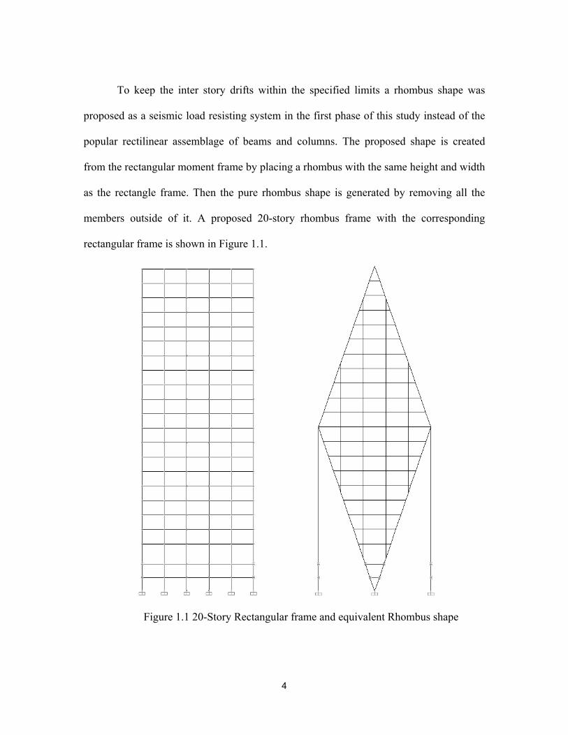
To keep the inter story drifts within the specified limits a rhombus shape was
proposed as a seismic load resisting system in the first phase of this study instead of the
popular rectilinear assemblage of beams and columns. The proposed shape is created
from the rectangular moment frame by placing a rhombus with the same height and width
as the rectangle frame. Then the pure rhombus shape is generated by removing all the
members outside of it. A proposed 20-story rhombus frame with the corresponding
rectangular frame is shown in Figure 1.1.
Figure 1.1 20-Story Rectangular frame and equivalent Rhombus shape

5
The idea behind this shape is to utilize the advantage of both the rectangular
moment frames and concentrically braced frames. The first type of framing system uses
the flexural stiffness of the members to gain lateral stiffness; while in the later type,
internal axial stiffness of the diagonals are the main sources for lateral stiffness. Different
framing systems are discussed briefly in the background section of this chapter.
To study the performance of the proposed rhombus shape, a wide range of steel
frames are selected with different height-to-width ratios. These frames represent low-rise
to high-rise buildings. Rhombus shape is compared with rectangular shape under
different earthquake excitations. As low-rise buildings are usually vulnerable to high
frequency earthquake and high-rise buildings are vulnerable to low frequency earthquake,
four different earthquakes are selected with wide range of frequency content. These are
Elcentro (1940), Northridge (1994), Parkfield (1966) and two data for Kocaeli (1999)
earthquake.
In the second phase of this study the concept of eccentrically braced frame (EBF)
is presented. The energy dissipation characteristic of the “link” of an EBF system is tried
to be incorporated in the frame system in the form of semi-rigid connections. In this part
of the study hybrid frames with rigid and semi-rigid connections are analyzed. The effect
of semi-rigid connections on global behavior of the hybrid rectangular and rhombus
frames are compared with the rigid frames. The eccentrically braced frame system and
the semi-rigid connections are briefly discussed in the background section.

6
1.2 Background
1.2.1 Moment Frames (MFs)
Moment resisting frames are the rectangular assemblage of beams and columns.
The beams are rigidly connected to the columns. Primarily the rigid frame action
provides resistance to lateral forces which develops bending moments and shear forces in
the frame members and joints. A moment frame cannot displace laterally without bending
the beams and columns due to its rigid beam-column connections. The bending rigidity
and strength of the frame members provide the lateral stiffness and strength for the entire
structure. For several reasons steel moment resisting frames have been popular in high
seismic regions. It is viewed as a highly ductile system among all the structural systems.
Also, large force reduction factors are assigned to design earthquake forces in building
codes. No bracing members are present to block the wall openings which provide
architectural versatility for space utilization. But, compared to other braced systems
moment frames generally required larger member sizes than those required only for
strength alone to keep the lateral deflection within code approved drift limits. Again, the
inherent flexibility of the system may introduce drift-induced nonstructural damage under
earthquake excitation than with other stiffer braced systems. Even these perceptions
regarding the expected performance of steel moment frames in energy dissipation under
lateral loads was sacrificed after the 1994 Northridge earthquake when the steel moment
frames did not perform as expected. Brittle failures occurred at beam-column connections
which challenge the assumption of high ductility of the system (Michel Bruneau et al.
1998).

7
Moment frames are composed of beam, column, and panel zone. Panel zone is the
portion of the column contained within the joint region at the intersection of beam and
column. In traditional analysis moment frames are often modeled with dimensionless
nodes which are the intersection of beam and column members. Such models do not
consider panel zone. But ductile moment frames require explicit consideration of panel
zone. Depending on the yield strength and the yield thresholds, the beam, column and
even panel zone could contribute to the total plastic deformation at the joint. A structural
component considerably weaker than the other framing into the joint will have to provide
the needed plastic energy dissipation. Those structural components expected to dissipate
hysteretic energy during an earthquake must be detailed to allow the development of
large plastic rotations. Plastic rotation demand is typically obtained by inelastic response
history analysis. Without considering panel zone plastic deformations it was expected
that the largest plastic rotations in the beams are 0.02 radian (Tsai 1988, Popov and Tsai
1989). After the Northridge earthquake the required connection plastic rotation capacity
was increased to 0.03 radian for new construction and for post earthquake modification of
existing building it was 0.025 radian (SAC1995b).

8
1.2.2 Concentrically Braced Frames (CBFs)
The concentrically braced frame is a lateral force resisting system. It is an
efficient frame system marked by its high elastic stiffness which is commonly used to
resist wind or earthquake loadings. The system achieves high stiffness by its diagonal
bracing members which resist lateral forces by using higher internal axial actions and
relatively lower flexural actions. Diagonal bracings form the main units which provide
lateral stiffness in a CBF system. Braces can be in the form of I-shaped sections, circular
or rectangular tubes, double angle attached together to form a T-shaped section, solid T-
shaped sections, single angles, channels and tension only rods and angles. Bracing
members are commonly connected with other members of the framing system by welded
or bolted gusset plates. The CBF design method generally focuses on dissipating energy
in the braces such that the connection is designed to remain elastic at all times. To
maximize the energy dissipation, the brace connections should be designed to be stronger
than the bracing members they connect so that the bracing member can yield and buckle
(Michel Bruneau et al. 1998). Some common CBF systems are shown in Figure 1.2.

9
Figure 1.2 Typical CBF configurations
CBF systems are considered to be less ductile seismic resistant structure as
compared to other systems due to failure of the bracing members under large cyclic
displacements. These structures can experience large story drift after buckling of bracing
members, which in turn may lead to fracture of bracing members. Recent analytical
studies have shown that CBF system designed by conventional elastic design method can
undergo severe damage under design level ground motions (Sabelli, 2000). Current
seismic codes (ANSI, 2005a) has provisions to design ductile CBF which is also known
as Special Concentrically Braced Frames (SCBFs).

10
1.2.3 Eccentrically Braced Frames (EBFs)
The eccentrically braced frame is a combination of concentrically braced frame
and moment resisting frame. The EBF combines individual advantages of each frame and
minimizes their respective disadvantages. It possesses high elastic stiffness, stable
inelastic response under cyclic lateral loading and excellent ductility and energy
dissipation capacity (Michel Bruneau et al. 1998). Eccentric braced frames utilize both
the axial loading of braces and flexure of beam sections to resist the lateral forces. It
addresses the need for a laterally stiff framing system with large energy dissipation
capabilities under large seismic forces. The key distinguishing feature of an EBF is the
isolated segment of a beam termed as “link.” A typical EBF consists of a beam, one or
two braces and columns. Its configuration is similar to other conventional braced frames
with the exception that each brace must be eccentrically connected to the frame.
Eccentric connection introduces shear and bending in the beam adjacent to brace. The
short segment of the frame where those forces are concentrated is the “link.” All inelastic
activity is intended to be confined to the properly detailed link. Links act as structural
fuses which dissipate seismic input energy without much degradation of strength and
stiffness and thereby transfer less force to the adjacent columns, beams and braces.
Common EBF arrangements are given in Figure 1.3.

11
Figure 1.3 Typical EBF configurations
Lateral stiffness of the EBF is a function of the ratio of link length to the beam
length. As the link becomes smaller the frame becomes stiffer approaches the stiffness of
CBF. And as the link becomes longer the frame becomes more ductile approaching to the
stiffness of a moment frame.
1.3 Literature review
PRE-NORTHRIDGE DESIGN
The presumed ductility of the discussed framing systems are dependent on the
connection properties. The welded moment connections were popular in North American
seismic regions before Northridge earthquake. By the 1960s the building industry was
frequently using an alternative connection detail with a bolted web connection and fully
welded flanges. To see the plastic behavior of these moment connections the first test was
conducted in 1960s. Popov and Pinkney (1969) tested 24 beam column joints.
Specimens with welded flanges and bolted connections showed superior inelastic

12
behavior compared with the cover plated moment connection and the fully bolted
moment connection due to the fact of slippage of the bolts which causes visible pinching
of the hysteresis loops under cyclic loading (FEMA-355e) (Michel Bruneau et al. 1998).
In 1970s, welded flanges-bolted web connections with fully welded connections
are compared (Popov and Stephen 1970) and the fully welded connection exhibited more
ductile behavior. Four out of five bolted webs failed abruptly. Popov and Stephen (1972)
also concluded that “The quality of workmanship and inspection is exceedingly important
for the achievement of best results (Michel Bruneau et al. 1998).”
Popov et al. (1985) tested eight specimens. The test mainly emphasize on panel
zone behavior with W18 beams. As per the authors, during the welding procedure: “the
back-up plates for the welds on the beam flange-to-column flange connections were
removed after the full-penetration flange welding was completed and small cosmetic
welds appeared to have been added and ground off on the underside (FEMA-355e).”
The tests by Tsai and Popov (1987) and Tsai and Popov (1988) indicated some
prequalified moment connections in ductile moment frames with W18 and W21 similar
in depth to those tested by Popov and Stephen (1971), were not as ductile as expected.
Before developing adequate plastic rotations, specimens with welded flanges-bolted web
connections failed abruptly. Only four out of eight specimens achieve desirable beam

13
plastic rotation. Authors realized about the quality control as an important factor (FEMA-
355e)
Engelhardt and Husain (1993) conducted 8 tests to investigate the effect of the
ratio of Zf /Z on rotation capacity using W21 and W24 beams, where Zf is the plastic
modulus of the beam flanges and Z is the plastic modulus of the entire beam. They could
not find any relation between Zf /Z with amount of hysteretic behavior developed prior to
failure. But, interestingly some of the specimens showed lack of ductility. This study also
compared their results with past experimental data. Assuming that connections must have
a beam plastic rotation capacity of 0.015 radian to survive under severe earthquake, they
found none of the specimens could provide that amount (Michel Bruneau et al. 1998).
Before Northridge earthquake most of the beam-column connections in a moment
resisting frames were detailed to be able to transfer plastic moment of the beams to the
columns (Roeder and Foutch 1995). Thus, relatively lighter column and beam sizes were
sufficient for those frames to resist seismic forces. With time many engineers concluded
that it was economically advantageous to limit the number of bays in a frame designed as
ductile moment frame. Prior to the Northridge earthquake even some engineers
frequently designed building with only four single-bay ductile moment frames with two
in each principal direction. This trend results with the loss in structural redundancy. In an
addition these single-bay moment frames required considerably deeper beams and
columns with thicker flanges than the multi-bay ones previously used to resist the same
14
lateral forces. It provided an opportunity to investigate potential size effects (Michel
Bruneau et al. 1998). Roeder and Foutch (1996) compiled all the test results for pre-
northridge connections and found that the expected ductility decreases with the deeper
sections. Bonowitz (1999a) found the same results from the tests conducted after
Northridge earthquake (FEMA-355e)
POST-NORTHRIDGE DESIGN
Numerous factors have been identified which were potentially contributed to the
poor seismic performance of the pre-Northridge steel moment connections. Failure
happened due to different combinations of those factors: workmanship and inspection
quality; weld design; fracture mechanics; base metal elevated yield stress; welds stress
condition; stress concentrations; effect of triaxial stress conditions; loading rate; amd
presence of composite floor slab (Michel Bruneau et al. 1998).
Numerous solutions to the moment frame connection problems have been
proposed. Two key strategies have been developed to overcome the problem. One of
them is to strengthening the connection and the other is weakening the beam ends which
is framed into the connection. Both strategies effectively move the plastic hinges away
from the face of the column (Michel Bruneau et al. 1998).
Satisfactory performance requires that a connection should be capable of
developing a beam plastic rotation of 0.03 radian with a minimum strength equal to 80
percent of the plastic strength of the girder. These are the acceptance criteria suggested in

15
SAC interim guidelines (1995b). As the minimum requirement it was recommended that
experimental validation of proposed connection be done with the qualification tests in
compliance with the ATC-24 loading protocol (ATC1992).
SEMI-RIGID CONNECTIONS
A connection in a moment frame will termed as partially restrained if it
contributes to a minimum 10% of the lateral deflection or the connections strength is less
than the weaker element of connected members (FEMA-356). It is presumed that in the
Northridge earthquake, partially restrained connections could result in a better
performance to provide flexibility in the structure. Proper placing of semi-rigid
connections along with the rigid connection could improve the performance of moment
frames. Modeling process of semi-rigid connections in a beam column joint is described
in Chapter 4.
Kasai et al. (1999) and Maison et al. (2000) studied the effect of semi-rigid
connections within the SAC program. But, in those studies all the connections were
considered as partially restrained (FEMA-355c). However, the knowledge about the
effect of semi-rigid connections in a hybrid frame is limited. Built on the pioneer work of
Radulova (2009), this research aims to study the seismic performance of fully rigid and
hybrid rhombus and rectangular framing systems.

16
1.4 Objective of the Present Study
The objective of this study is to identify the effect of building shape on its
seismic performance. Thus rhombus shape frames are selected based on engineering
intuition and they were subjected to five earthquake records from four different frequency
earthquake. The control frame was selected to be the rectangular frame based on the SAC
Frame (FEMA-355) geometry. The aspect ratio and geometrical dimensions were varied
to obtain their earthquake response which included lateral sway, inter-story drift and
member forces. In the second phase of the study, high rise hybrid frames with rigid and
semi-rigid connections are subjected to earthquake forces to identify the effect of semi-
rigid connections on the global behavior of the frames.
1.5 Scope of the Study
The scope of this study was limited between Rhombus and Rectangular shape
frames. For both rhombus and rectangular; three, nine, twelve and twenty story frames
are modeled with all the connections being rigid. The frames are analyzed under 5
different seismic excitation records only. These are for Elcentro, Northridge, Parkfield
and two records for Kocaeli earthquakes. The results compared between the two shapes
includes lateral sway, inter story drifts and internal forces of the members. Semi-rigid
connection property has been incorporated only on the 20-story frames. Bi-linear
moment-rotation curve has been used to define semi-rigid connection properties. No
ultimate moment provision has been considered in moment-rotation curves. To create the

17
hybrid frames semi-rigid connections are placed only on the mid levels of the frames,
based on Radulova (2009).
1.7 Organization of the Present Study
This study is organized as per objectives. Background about this research is
narrated in Chapter 1. It includes previous earthquakes effects, seismic regulations, brief
discussion on connections, different framing systems and objectives of the study. Chapter
2 describes about the different analysis procedures. In Chapter 3, the proposed rhombus
frames are compared with the corresponding rectangular frames under different
earthquake records. Modeling process of semi-rigid connection is described in Chapter 4.
It also includes earthquake response of hybrid frames with rigid and semi-rigid
connections. Comments and discussions on the results are described in Chapter 5 along
with the recommendations for future work in this area.

18
CHAPTER 2
BACKGROUND ON FRAME ANALYSIS
2.1 Introduction
Structural analysis uses the laws of physics and mathematics to predict the
performance and behavior of structures. Actual behavior of a structure is complicated, but
different level of idealization could decrease the complexity. Here in this chapter the term
analysis will mainly deal with the procedures and guidelines to obtain the member
strength and deformation demands of a structure under seismic load. In the first part of
this chapter different analysis methods proposed by Federal Emergency Management
Agency (FEMA), National Earthquake Hazards Reduction Program (NEHRP) will be
overviewed. Then general discussion on some analysis procedure will be given briefly
and at last some solution techniques will be discussed.
2.2 Analysis Methods
Different degrees of complexity due to geometry of the structure along with the
material behavior are associated in the structural response under seismic excitation.
Depends on the needed accuracy different types of idealizations are proposed in the
evaluation of structural response. FEMA-355f considered four elastic and three inelastic
analysis procedures implemented by FEMA-273, NEHRP Guideline (1997) for
performance evaluation of steel moment resisting frames.

19
2.2.1 Elastic Analysis Methods
The proposed elastic analysis procedures are equivalent lateral force and modal
analysis by FEMA-302, FEMA-273 linear static and linear dynamic methods and linear
time history analysis procedures (FEMA-355f).
In the equivalent lateral force method, base shear is calculated based on seismic
response coefficient and total dead load with applicable portion of other loads. This base
shear is distributed to different floor levels and the response will be calculated from the
static analysis (FEMA-355f).
FEMA-273 linear static procedure uses the same background as the equivalent
lateral load method to calculate the seismic load. Instead of design base shear this method
brings in the term “pseudo lateral load” which is the final product after using different
modification factors. The “pseudo lateral load” is selected in a way so that the response
due to this load will be approximately same as from nonlinear time history analysis
(FEMA-355f).
Linear time history procedure uses two methods in calculating structural response.
In one method modal analysis and mode superposition is used which is explained later in
this chapter. In another method this procedure uses direct integration technique in
calculating seismic response. Some common integration techniques namely Newmark
and Wilson methods are discussed at the end of this chapter.

20
2.2.2 Inelastic Analysis Methods
The considered inelastic analysis procedures are FEMA-273 nonlinear static
procedure, capacity spectrum procedure (Skokan and Hart, 1999) and nonlinear time
history analysis (FEMA-355f).
FEMA-273 nonlinear static procedure is also known as the static pushover
analysis. In this method inelastic material behavior with P-∆ effects are included. These
effects are briefly discussed later. In this method a target displacement is assigned at any
point of the structure and then the structure is pushed with a increasing lateral load until
the target displacement is achieved to that point or the structure collapses (FEMA-355f).
Capacity spectrum method is mainly applicable for reinforced concrete structures
(ATC, 1996) and thus beyond the scope of this study. And the nonlinear time history
analysis procedure is same as the linear time history analysis, only material nonlinearity
along with the geometric effects should be considered in evaluation of structural
response. Some key terms of these analysis procedures are explained in the following
sections.
2.3 First Order Elastic Analysis
The first order elastic frame analysis considers the structural behavior as linear
under any type of loading. This analysis method does not consider the geometric effects
as member and the structural deflections (P-Δ and P-δ effects) as well as material

21
nonlinearity. It assumes that the displacement will be very small and therefore the second
order effects due to geometrical changes are ignored. And thus the stiffness matrix is
constant for the members independent of applied axial forces. The deflection is
proportional with the applied load, ie with increasing load the displacement will also
increase which can be expressed as a straight line as shown in Figure 2.1.
Figure 2.1 Generalised Load-Displacement curve for different types of analysis
The initial slopes of other types of analyses are coincided with it. It is because at
lower loads the structures do not develop any secondary effects in geometry and material
properties.
2.4 Second Order Elastic Analysis
Second order elastic analysis considers the geometric effects which are due to the
member and structural deflections named as P-δ and P-Δ effects respectively. Structural
response due to the second order elastic analysis is presented in the load-displacement

22
curve shown in Figure 2.1. Initially it follows the path of linear analysis, but as the
loading increased to produce sufficient geometric effect it starts to deviate from linear
analysis to show the effect of geometric nonlinearity. Figure 2.2 shows P-δ and P-Δ
effects, which is the cause for this geometric nonlinearity.
Figure 2.2 P-δ and P-Δ effects
These geometric effects produce higher internal forces due to axial loads. The
stiffness matrix needs to be adjusted to reflect these effects and the corrections develop
additional deflection. To account this problem the system reaches in equilibrium in an
iterative process. As the stiffness matrix and thus the structural response are dependent on
the deflected shape of the frame, principle of superposition is not applicable in second
order elastic analysis. As material nonlinearity is not considered, this method over
predicts the collapse load.
P P
δ
Δ

23
P-δ EFFECT
When a member deforms, it affects the stiffness of that member and additional
moment will be developed in the member. This second order effect due to deflection
along a member and the axial force is termed as P-δ effect.
P-Δ EFFECT
If a structure deflects significantly, then the original geometry of the structure
cannot be used to formulate the transformation matrix due to change in nodal coordinates.
This is known as P-Δ effect.
2.5 Inelastic Analysis
Material yielding and instability of structural members have significant effect to
control the ultimate load. If the material nonlinearity is included in the second order
elastic analysis, it would become the inelastic analysis. Nonlinearity in the inelastic
analysis exists in two forms – geometric nonlinearity and material nonlinearity.
Material start yielding at the outer fiber of the section when the elastic moment
reaches to yield moment value My. Material nonlinearity come into affect at this point
and after that with application of additional load, yielding will spread over the section
from outer fiber to plastic neutral axis. The section will continue yielding until the whole
section is yielded to develop full plastic moment Mp. This nonlinearity can be
incorporated to the analysis mainly by two approaches. In the first approach plastic
hinges are assumed to form at the two ends of a member i.e. all the material nonlinearity

24
is basically lumped at the two ends of a member. This is known as concentrated plasticity
(plastic hinge, lumped plasticity) approach. Another approach assumes the plasticity over
the whole member known as distributed plasticity (plastic zone) approach (Chan and
Chui, 2000).
CONCENTRATED PLASTICITY APPROACH
Concentrated plasticity approach ignores the progressive yielding along the
member length. It assumes the material nonlinearity to be lumped in a small region of
zero length (Yau and Chan, 1994). It deals with the cross section plastification, which
starts at the outer most fiber of the section and ends up with the formation of a hinge at a
given point. It assumes that the hinges will form only at the ends and the remaining part
of the member will remain elastic. Mashary and Chen (1991) and Yau and Chan (1994)
modeled this material nonlinearity by using zero length spring at the member ends. Many
other methods are proposed for computer simulation of this hinge property. This
approach is easier to apply and significantly save computation time than the distributed
plasticity approach. Commonly used methods for modeling plastic hinges are elastic-
plastic hinge method, column tangent modulus method, beam-column stiffness
degradation method, beam-column strength degradation method and end spring method.
DISTRIBUTED PLASTICITY APPROACH
This approach assumes yielding will be distributed over the length of the member
and the cross section. This method discretized structure into many elements and each
section is further divided into small fibers in an attempt to monitor stress and strain for all
members. Initial imperfections and residual stresses can be included by assigning stresses

25
to each fiber before loading which can be varied along the side and thickness of the
section (Chan, 1990). The distributed plasticity approach is more accurate than the
concentrated plasticity approach as fundamental stress-strain relationship is directly
applied for the computation of forces. This approach requires considerable amount of
computation time and huge memory to store data. Thus this method is suitable to analyze
simple structures. Commonly used methods for this approach are traditional plastic zone
method and simplified plastic zone method.
2.6 Dynamic Analysis of frame
Structural dynamics deal with the behavior of structure under dynamic loading. A
static load is one which does not vary with time. A dynamic is any load which changes its
magnitude, direction or position with time. If it changes very slowly, the structures
response may be determined using static analysis but if the loading varies with time
quickly (corresponding to the structures time period), the structures response must be
determined using dynamic analysis. Here in this study dynamic term will use for seismic
loads.
A structural dynamic analysis differs from the static analysis in two ways. Firstly
in a dynamic problem both the applied force and the resulting response in the structure
are time variant, i.e. function of time. It does not have a single solution like the static
problem. For complete evaluation of structural response one has to investigate the
solution over a specific interval of time. And the other one which is the most important

26
feature in dynamic analysis is the act of inertia force. If a load is applied in a structure
dynamically, there will be time variant deflection in the structure which will cause
acceleration and thus inertia force will be induced. Magnitude of the inertia force depends
on the acceleration and mass characteristics of the structure. Unlike static analysis,
dynamic problems significantly depend on mass and damping. Three components, mass
and damping together with the stiffness characteristics are required to write the equations
of motion. Mass will be calculated from all the loads that the structure carries and
members self-weight. This mass can be lumped at the joints or distributed over the
member. Stiffness is basically provided by the structural components of a system. And
the third component Damping is the energy dissipation properties of a material or system.
It is a process by which a free vibration could steadily diminishes in amplitude and
finally come to rest. In a vibrating system the energy could be dissipated by various
mechanisms and often more than one mechanism can be present at the same time.
The equivalent lateral load approach discussed before transforms dynamic force
into static forces. But, it cannot reflect the true dynamic response, as characteristic of
resonance cannot be explained in a static approach. To include all the dynamic effects in
the analysis, mode superposition and modal analysis is a widely accepted method for
linear systems. Different types of direct integration methods are used to solve both linear
and nonlinear dynamic problem numerically. Different methods are briefly discussed in
the following sections.

27
2.7 Modal Analysis
Modal analysis in structural dynamics is used to determine the natural mode
shapes and frequencies of a structure. It is a convenient method for calculating the
dynamic response of a linear structural system. The response of a MDF system under
externally applied dynamic load can be described by N differential equations in the
following form,
[m] {ü} + [c]{ů} + [k]{u} = {p(t)}, where
[m] is the mass matrix,
[c] is the damping matrix,
[k] is the stiffness matrix of the system,
{p(t)} is the externally applied dynamic force matrix, and
{u}, {ů}, {ü} denotes displacement, velocity and acceleration matrix.
The main approach of this method for dynamic analysis is to change N set of
coupled equations of motion into N uncoupled equation for a multiple-degree-of-freedom
system. Based on the number of DOF, a MDF system has multiple characteristic
deflected shapes. Each characteristic deflected shape is called a natural mode of vibration
of the MDF system denoted by øn. The displacement {u(t)} of the system can be
determined by the superposition of modal contributions. i.e. {u(t)} = ∑=
N
n 1
qn(t)øn, where
qn(t) = modal coordinates. Deflected shape øn does not vary with time. The equation,
[k]øn = ωn2[m]øn , is the matrix eigen value problem where ωn is the natural frequency and
28
øn is the natural modes of vibration of the system (Chopra, A.K. 1995). This equation has
a non trivial solution if,
0][][ 2 =− mk nω ,
This is known as the frequency equation, because after expanding the determinant
it creates a polynomial of order N in ωn2. This equation has N number of real and positive
roots for ωn2 i.e. N number of natural vibration frequencies, started with ω1 be the
smallest and ωn be the largest. If applied force {p(t)} can be written as [s]p(t) with spatial
distribution is defined by [s], then the spatial distribution is expanded to its modal
components {sn}. where, {sn} = Γn [m]øn. Then the equation could be transformed to
uncoupled equations in modal coordinates and the solution for the modal coordinate is,
qn(t)= ΓnDn(t), where Dn is governed by the equation of motion for nth-mode SDF system
of the nth mode of the MDF system. The contribution from this mode to modal
displacement is, {un(t)} = ønqn(t) = ΓnønDn(t). And the equivalent static force associated
with the nth mode response is, {fn(t)}={sn}{An(t)}, where An(t) = ωn2Dn(t), is the pseudo
acceleration. The nth mode contribution to any response is determined by the static
analysis for force {fn}. By combining all the response contributions from all the modes
gives the total dynamic response (Chopra, A.K. 2007).
2.8 Step-by-Step Integration
Analytical solution of a dynamic problem is not possible in cases where the
physical properties like geometry and elasticity of material do not remain constant. The
stiffness coefficient can be changed with yielding of materials or by significant change in
29
axial force which will cause the change in geometric stiffness coefficient. The applicable
method for the analysis of nonlinear system is the numerical step-by-step integration,
which is also applicable to linear systems. The main approach of this method is to divide
the response history into short time increments and then the response is calculated during
each increment assuming it as a linear system with the properties determined at the start
of each increment. The properties are updated at the end of each interval based on the
deformation and stress, and thus the nonlinear system is idealized as a collection of
changing linear systems. In 1959, Newmark N.M. developed a method of computation
for dynamic problems in structure. Later modifications are made to this method based on
the stability, accuracy etc. Some popular methods are briefly discussed in the following
sections.
2.8.1 Newmark’s Method
In this method it is assumed that at time i the values of displacement, velocity and
acceleration is known and by numerical integration it can be estimated for time i+1, if the
time increment, ∆t is very small. Newmark introduce two parameters γ and β to indicate
the proportion of acceleration that will enter into the equations for displacement and
velocity (Newmark N.M. 1959). The adopted equations are,
ui+1 = ui + (∆t) ůi + [ (0.5 – β)(∆t)2] üi + [ β(∆t)2 ] üi+1 (2.1)
ůi+1 = ůi + [ (1 – γ) ∆t ] üi + (γ ∆t) üi+1 (2.2)
The two parameters γ and β in the above two equations are responsible for the
stability and accuracy of the system. If γ is taken as zero, a negative damping will result,
which will produce a auto vibration from the numerical method. Again if γ is greater

30
than21 , a positive damping addition to the real damping will be introduced to reduce the
magnitude of the response. So, generally γ is taken as equal to 21 . And better results are
obtained with values of β range between 61 to
41 (Newmark, N.M. 1959). Two popular
special cases for Newmark’s method are as follows -
2.8.1.1 Average Acceleration Method
Figure 2.3 Average acceleration
If there is no variation of acceleration over a time step and the value is constant,
equal to the value of average acceleration, then,
ü ( )τ = 21 (üi+1+ üi) . If ( )τ = ∆t , this will yield
ůi+1 = ůi + 21 ∆t (üi + üi+1) , and ui+1 = ui + (∆t) ůi +
41 (∆t)2 (üi + üi+1).
τ
Δt
ü
t ti ti+1
üi+1
üi
31
These two equations are same as equation 2.1 and 2.2, if γ =21 and β =
41 . For
this method, maximum velocity response is correct whether value of β other than 41 will
cause some error (Newmark N.M. 1959). From stability point of view Newmark’s
method is stable if,
βγπ 2
12
1−
≤Δ
nTt (2.3)
Where, Tn is the natural time period of the system.
For, γ =21 and β =
41 , ∞≤
Δ
nTt ie average acceleration method is unconditionally stable.
2.8.1.2 Linear Acceleration Method
Figure 2.4 Linear acceleration
If the variation of acceleration is linear over a time step, then,
ü ( )τ = üi + tΔτ (üi+1 – üi). If ( )τ = ∆t , this will yield
τ
Δt
ü
t ti ti+1
üi+1
üi

32
ůi+1 = ůi + 21 ∆t (üi + üi+1) , and
ui+1 = ui + (∆t) ůi + (∆t)2 (31 üi +
61 üi+1).
These two equations are same from equation 2.1 and 2.2, if γ =21 and β =
61 .
Equation 2.3 shows that the linear acceleration method will be stable, if 551.0≤Δ
nTt . And
so this method is conditionally stable. But stability criteria have not imposed any rule in
selecting time step. In general by taking short integration interval, a good accuracy can be
achieved from unconditionally stable linear acceleration method.
2.8.2 Wilson θ Method
E.L.Wilson modified the conditionally stable linear acceleration method into
unconditionally stable. His proposed method is known as Wilson θ Method. This method
assumes that the acceleration will vary linearly over an extended interval, δt = θ∆t.
Figure 2.5 Linear variation of acceleration over extended time steps
t Δt
ü
ti ti+1
üi+1
üi
ti+θ
Δüi δüi
δt= θ Δt

33
The parameter θ in this method determines the accuracy and the stability
characteristics of the numerical analysis. For θ = 1, this method will turn into Newmark’s
standard linear-acceleration method. For θ ≥ 1.37, Wilson’s method becomes
unconditionally stable.
2.8.3 Hilber-Hughes-Taylor Method
In order to introduce numerical damping into Newmark’s method without
affecting the accuracy Hilber, Hughes and Taylor introduce the parameter α. Where,
γ = ( )221 α− and β = ( )
41 2α−
The range of this parameter is from - 31 to 0. If α = 0, then this method turns into
Newmark’s average acceleration method. This would give the higher accuracy but it may
produce excess vibrations in the higher modes. Decreasing value of α will increase the
amount of numerical damping which will mainly damp the higher frequency modes.
Sometimes it is required for a nonlinear solution to converge with using negative α. value
(SAP2000).

34
CHAPTER 3
EFFECT OF FRAME SHAPE AND GEOMETRY ON SEISMIC PERFORMANCE
3.1 Introduction
The SAC joint venture between the Structural Engineers Association of California
(SEAOC), the Applied Technology Council (ATC), and the California Universities for
Research in Earthquake Engineering(CUREe), proposed 3-story, 9-story and 20-story
frames. Several steel frames with these SAC dimensions are used for this study. These
frames represent from low-rise to high-rise buildings. Besides these, a 12-story frame is
also modeled. Initially all buildings are modeled as Rectangular Moment Frame with all
connections being rigid. Later, a Rhombus shape has been proposed to see the effect of
shape on the global behavior of the frame. The Rhombus shape has been constructed by
placing the Rhombus building inside the Rectangular frame. This Rhombus shape frame
has the same height and width ratios as the Rectangular shape. All the member sizes,
joint loads and uniformly distributed loading were kept the same for both the shapes.
All the frames are analyzed under five different earthquake excitation data. These
earthquakes reflect a wide variation in frequency content. For each height, results are
compared between Rectangular and Rhombus shapes. Results include lateral sway, drift,

35
top displacement and member forces. Effect of height-to-width ratios on the
fundamental properties of the structure is also observed.
Total eight rigid frames are developed. To describe the results a general building
designation is adopted for convenience,
_S – H_W_H/W- OP( _,/ _ ) - EQ , where
S = story
H = the height of the frame
W = the width of the frame
H/W = the height-to-width ratio of the frame
OP = out put, which can be member forces or displacement
AF = axial force
SF = shear force
BM = bending moment
TDUx = top node displacement along X-direction
MDUx = maximum displacement along X-direction
LDr = Lateral inter story drift
RMR = Rigid Rhombus frame
RCR = Rigid Rectangular frame
EQ = earthquake
ELC = El Centro earthquake
NRG = Northridge earthquake

36
PKF = Parkfield earthquake
KCL1 = Afyon Bay record for Kocaeli earthquake
KCL2 = Aydin record for Kocaeli earthquake
The building designation follows: 20S – 289_100_2.89 – TDUx (RMR, RCR) –
ELC, which will describe a 20 story frame with height-to-width ratio of 2.89 where the
height and the width are 289 ft and 200 ft, respectively. The out put describes top
displacement along X- direction for both the Rhombus shape and Rectangular shape with
all the connections being rigid, and the results are for El Centro earthquake. Thus, BM(
RMR/RCR) will describe bending moment as out put. And the result will be the ratio of
bending moment for the Rhombus shape and the Rectangular shape.
3.2 Three Story Frame
The analysis starts with the modeling of a three story frame. This three story 4-
bay frame is used to observe the effect of earthquake excitation on low rise structures.
The rectangular frame is 120ft wide with 30ft bay dimension and the total height of the
building is 39 ft. These dimensions are taken from SAC 3-Story building. All the member
sizes are W14 X 283. All the connections are considered to be rigid. Total dead load and
25 percentage of live load are considered for calculating member mass. Load calculations
are described in Appendix G. The 3-story rectangular frame with corresponding rhombus
shape is shown in Figure 3.1. These frames are analyzed under five different earthquake
excitation records. The results are plotted in the Appendices A through F of this report as
an attempt to show the comparison between the two shapes.

37
Figure 3.1 Three-Story Rectangular and Rhombus frame
Both of these models are analyzed under modal analysis and the corresponding
first couples of mode shapes are given below.
(a) (b)
Figure 3.2 First two Mode Shapes for 3-Story Rectangular Frame (a) Mode 1, (b) Mode 2
(a) (b)
Figure 3.3 First two Mode Shapes for 3-Story Rhombus Frame (a) Mode 1, (b) Mode 2
These mode shapes are obtained from the SAP2000 software. Corresponding
natural time period and frequencies for first ten modes are tabulated in the following
table.

38
Table 3.1 Modal period and frequencies for 3-Story Frames (SAP 2000)
Mode 3S – 39_120_0.325 – (RCR) 3S – 39_120_0.325 – (RMR)
Period Frequency Period Frequency (sec) (Hz) (sec) (Hz)
1 0.56324 1.7754 0.28961 3.4529 2 0.17082 5.8543 0.17561 5.6943 3 0.0964 10.374 0.11076 9.0288 4 0.05435 18.4 0.06529 15.317 5 0.05406 18.499 0.0555 18.019 6 0.05368 18.63 0.05294 18.888 7 0.0479 20.877 0.04959 20.167 8 0.04613 21.679 0.03818 26.191 9 0.04231 23.637 0.03408 29.344
10 0.03836 26.068 0.02795 35.777
3.3 Nine Story Frame
The nine story frame has been modeled with the SAC 9-Story building
dimensions. This nine story 5-bay frame is used to observe the effect of earthquake on
medium high-rise buildings. The rectangular frame is 150ft wide with 30ft bay
dimension, and the total height of the building is 134 ft with a 12ft basement. All the
member sizes are W14 X 283. All the connections are considered to be rigid. Total dead
load and 25 percentage of live load are considered for calculating member mass. Load
calculations are described on Appendix G. The 9-story rectangular frame with equivalent
rhombus shape is shown in Figure 3.4. These frames are analyzed under five different
earthquake excitation records. The results include top displacements, lateral sway, inter
story drifts and member forces. All the results are plotted in the Appendices A through F

39
of this report to compare the performance of individual shape under earthquake
excitations.
Figure 3.4 Nine-Story Rectangular and Rhombus frame
These models are analyzed under modal analysis and the first couples of mode
shapes are given in the following Figures.
(a) (b)
Figure 3.5 First two Mode Shapes for 9-Story Rectangular Frame (a) Mode 1, (b) Mode 2

40
(a) (b)
Figure 3.6 First two Mode Shapes for 9-Story Rhombus Frame (a) Mode 1, (b) Mode 2
The modal analysis is performed in the SAP2000 platform. Corresponding time
period and frequencies for first ten modes are tabulated in the following Table
Table 3.2 Modal period and frequencies for 9-Story Frames (SAP 2000)
Mode 9S – 134_150_0.893 – (RCR) 9S – 134_150_0.893 – (RMR)
Period Frequency Period Frequency (sec) (Hz) (sec) (Hz)
1 1.92246 0.52017 0.4332 2.3084 2 0.6213 1.6095 0.37677 2.6542 3 0.3527 2.8353 0.18268 5.474 4 0.23647 4.2289 0.17649 5.6662 5 0.17226 5.8051 0.13888 7.2004 6 0.16484 6.0667 0.12993 7.6968 7 0.16 6.25 0.12041 8.3047 8 0.15317 6.5286 0.1063 9.4078 9 0.1468 6.8121 0.08393 11.915
10 0.13315 7.5105 0.07483 13.364

41
3.4 Twelve Story Frame
The twelve story 5-bay frame is used to observe the geometric effect of frame
under earthquake excitation. The rectangular frame is 150ft wide with 30ft bay
dimension, and the total height of the building is 173 ft with a 12ft basement. All the
member sizes are W14 X 283. All the connections are considered to be rigid. Total dead
load and 25 percentage of live load are considered for calculating member mass. The 12-
story rectangular frame with corresponding rhombus shape is shown in Figure 3.7. These
frames are analyzed under five different earthquake excitation records. The out put
results include top displacement, lateral sway, inter story drift and member forces. All the
results are plotted in the Appendices A through F of this report as an attempt to show the
comparison between the two shapes.
Figure 3.7 Twelve-Story Rectangular and Rhombus frame

42
Both of these frames are analyzed under modal analysis. In the following Figures,
first couples of mode shapes are provided. These shapes are obtained from the SAP2000
software.
(a) (b)
Figure 3.8 First two Mode Shapes for 12-Story Rectangular Frame (a) Mode 1, (b) Mode 2
(a) (b)
Figure 3.9 First two Mode Shapes for 12-Story Rhombus Frame (a) Mode 1, (b) Mode 2

43
Corresponding time period and frequencies for the first ten modes are tabulated
below.
Table 3.3 Modal period and frequencies for 12-Story Frames (SAP 2000)
Mode 12S – 173_150_1.153 – (RCR) 12S – 173_150_1.153 – (RMR)
Period Frequency Period Frequency (sec) (Hz) (sec) (Hz)
1 2.51114 0.39823 0.5671 1.7634 2 0.82114 1.2178 0.53406 1.8725 3 0.47433 2.1082 0.25183 3.9709 4 0.32474 3.0794 0.22645 4.4159 5 0.24064 4.1556 0.19174 5.2154 6 0.20952 4.7728 0.16486 6.0658 7 0.20019 4.9952 0.1559 6.4144 8 0.18754 5.3323 0.1157 8.643 9 0.18752 5.3327 0.10739 9.3116
10 0.176 5.6818 0.09298 10.755
3.5 Twenty Story Frame
A 20story rectangular frame has been modeled with SAC 20-Story building
dimensions. This 20-Story 5 bay frame is used to observe the effect of earthquake on
high-rise buildings. The rectangular frame is 100ft wide with 20ft bay width and the total
height of the building is 289ft with two basement floor 12ft each. All the member sizes
are W24 X 131. All the connections are considered to be rigid. Total dead load and 25
percentage of live load are considered for effective seismic load. 20-story rectangular
frames with corresponding rhombus shapes are shown in Figure 3.10. Both of the frames
are analyzed with Modal analysis on the SAP2000 platform. First couples of modal

44
shapes obtained from modal analysis are given in Figure 3.11 and 3.12. Corresponding
time period and frequencies for first ten modes are given in Table 3.4. These frames are
analyzed under five different earthquake excitation records. The results include top
displacements, lateral sway, inter story drift and member forces. All the results are
plotted in the Appendices A through F of this report to compare the performance of
individual shape under earthquake excitation.
Figure 3.10 Twenty-Story Rectangular and Rhombus frames
45
(a) (b)
Figure 3.11 First two Mode Shapes for 20-Story Rectangular Frame (a) Mode 1, (b) Mode 2
(a) (b)
Figure 3.12 First two Mode Shapes for 20-Story Rhombus Frame (a) Mode 1, (b) Mode 2

46
Table 3.4 Modal period and frequencies for 20-Story Frames (SAP 2000)
Mode 20S–289_100_2.89–(RCR) 20S–289_100_2.89-(RMR)
Period Frequency Period Frequency (sec) (Hz) (sec) (Hz)
1 2.72965 0.36635 1.58828 0.62961 2 0.87486 1.143 0.48492 2.0622 3 0.49 2.0408 0.279 3.5842 4 0.34352 2.9111 0.25668 3.8959 5 0.31924 3.1324 0.22956 4.3562 6 0.2623 3.8125 0.18013 5.5514 7 0.24444 4.0909 0.15376 6.5037 8 0.20718 4.8266 0.13834 7.2287 9 0.17824 5.6103 0.11651 8.5827
10 0.17207 5.8116 0.10433 9.5849
3.6 Eathquake in consideration
Ground acceleration values in an earthquake vary with time in an irregular
manner. As a result, an earthquake is generally composed of infinite number of frequency
content. The non periodic acceleration time function can be represented by the Fourier
integral –
ωωπ
ω deFtu tig ∫
∞
∞−
−= )(21)(&&
A Fourier spectrum constitutes the representation of a time history into the
frequency domain. If üg(t) denotes ground acceleration in the time domain, the Fourier
spectrum of üg(t) is defined as
dtetuF tig∫
∞
∞−
−= ωω )()( &&
47
F(ω) represents ground acceleration in frequency domain. The amplitude of the
Fourier spectrum is used to identify the harmonic components of the earthquake that has
the largest amplitudes. These harmonic components are identified in terms of their
frequencies. The amplitude Fourier spectrum of an earthquake may be interpreted as a
measure of the total energy contained to that ground motion.
For this study four different earthquakes are used with a wide variety of frequency
range. El Centro and Northridge earthquakes represent the high-frequency range,
Parkfield earthquake is a medium-frequency earthquake. And two site records are
provided for low frequency Kocaeli earthquake.
3.6.1 Generated Earthquake
To observe the resonance effect on 20 story frames, a Sine wave, composed of
three different time period is generated; ie it consists of total three frequencies. Another
reason for constructing this imaginary earthquake is to verify the SeismoSignal software
about it’s capability to determine dominant frequencies, as the original frequency
contents for this generated data are known. Total time for the generated earthquake is
79.17 sec. It is constructed in a manner, so that in the first part, it will create resonance
with the 20 story rhombus frame, and the last part will create resonance with the 20 story
rectangular frame. From 0 ~ 10.92 sec, time period, T = 1.365 sec; frequency, f
=0.733Hz, with total 8 cycle. In this time range amplitude is almost three times higher
than the rest of the vibration. From 10.92 ~ 54.6 sec, time period, T = 5.46 sec;
frequency, f = 0.183Hz, with total 8 cycle. And from 54.6 ~ 79.17 sec, time period, T =

48
2.73 sec; frequency f = 0.366Hz, with total 9 cycle. The generated data is plotted in
Figure 3.13.
-0.4
-0.3
-0.2
-0.1
0
0.1
0.2
0.3
0.4
0 16 32 48 64
Time (sec)
Acc
eler
atio
n (g
)
Figure 3.13 Acceleration Time History of Generated Earthquake
Now, if this data is used in SeismoSignal software, it will give three dominant
frequencies as in Figure 3.14.
1st dominant, f = 0.183Hz,
2nd dominant, f = 0.733Hz, and
3rd dominant, f = 0.366Hz.

49
0
0.5
1
1.5
2
2.5
0 1 2 3 4 5Frequency (Hz)
Four
ier A
plitu
de
Figure 3.14 Fourier Spectrum of Generated Earthquake
In Figure 3.14, 0.183Hz is the 1st dominant frequency, because it covers most of
the time range in Figure 3.13. But the software does not consider only the time range.
That is why 0.733Hz is the second dominant instead of 0.366Hz (which is the second
large in terms of time range). 0.733Hz is the 2nd dominant, as the amplitude of
acceleration of that part is almost three times higher than the other.
To observe the resonance effect, 20S–289_100_2.89–(RMR) and 20S–
289_100_2.89–(RCR) frames are analyzed with this data. The resulted top displacements
of the two frames are shown in Figure 3.15. Figure shows, rhombus frame gives top
displacement in the first part of the total time range, as vibration frequency of that time
range is close to the natural frequency of the rhombus frame. And the rectangular frame

50
gives maximum top displacement at the last part of the total time, where vibration
frequency is close to the natural frequency of the rectangular frame.
-120
-104
-88
-72
-56
-40
-24
-8
8
24
40
56
72
88
104
120
0 16 32 48 64 80Time(sec)
Dis
plac
emen
t-Ux(
inch
)
-304.8
-244.8
-184.8
-124.8
-64.8
-4.8
55.2
115.2
175.2
235.2
295.2
Dis
plac
emen
t-Ux(
cm)
20S-289_100_2.89-TDUx(RMR)-genEQ 20S-289_100_2.89-TDUx(RCR)-genEQ
Figure 3.15 20S-289_100_2.89-TDux(RMR,RCR)-generated data
None of the frames experience higher top node displacement at the middle part of
the generated data, which one is the dominant frequency range for the total time. Again,
the rectangular frame which has resonance effect with the third dominant frequency,
gives a maximum top displacement value, which is more than double, than the top
displacement for the rhombus frame. So, in the following study, frequencies of the
earthquakes are defined as a range instead of giving emphasis on a single dominant
frequency.

51
3.6.2 ElCentro
The epicenter of the El Centro earthquake was in El Centro (Imperial Valley),
California. It occurred on May 18, 1940. The exact site, from where data was collected is
Imperial Valley, which is located 6 miles away from the epicenter. Nine people were
killed by the earthquake. At Imperial, 80 percent of the buildings were damaged to some
degree. In the business district of Brawley, all structures were damaged, and about 50
percent had to be condemned. The shock caused 40 miles of surface faulting on the
Imperial Fault, part of the San Andreas system in southern California. Total damage has
been estimated at about $6 million. The instrument that recorded the accelerogram was
attached to the El Centro Terminal Substation Building’s concrete floor. The record may
have under-represented the high frequency motions of the ground because of soil-
structure interaction of the massive foundation with the surrounding soft soil. The
earthquake magnitude was 7.1. The total duration was 53.5 seconds. The North-South
component of the El Centro earthquake was recorded with 0.02 second interval. First 30
seconds of the earthquake are used for time history analysis. Elcentro represents a high
frequency ground shaking. Its major frequency range is between 1.0 Hz to 2.25 Hz based
on the Fourier spectrum obtained from the SeismoSignal software. Figure 3.16 represents
the acceleration time history of El Centro earthquake in terms of the gravitational
acceleration, g. Figure 3.17 represents the Fourier transformation of the earthquake.
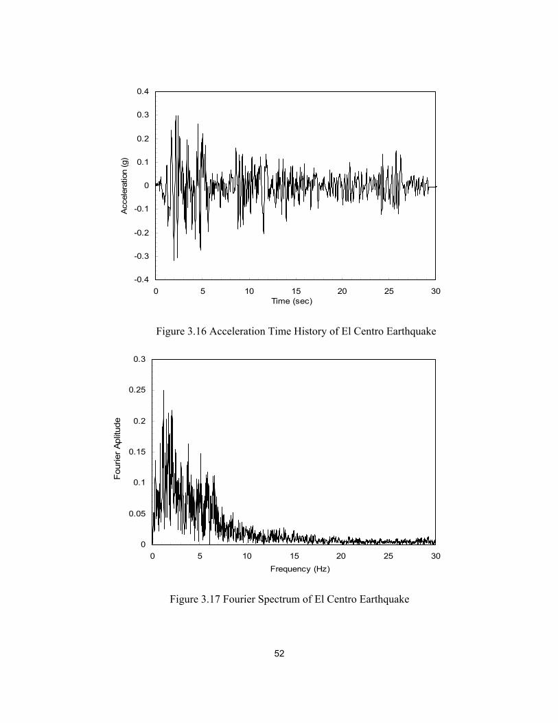
52
-0.4
-0.3
-0.2
-0.1
0
0.1
0.2
0.3
0.4
0 5 10 15 20 25 30Time (sec)
Acc
eler
atio
n (g
)
Figure 3.16 Acceleration Time History of El Centro Earthquake
0
0.05
0.1
0.15
0.2
0.25
0.3
0 5 10 15 20 25 30Frequency (Hz)
Four
ier A
plitu
de
Figure 3.17 Fourier Spectrum of El Centro Earthquake

53
Table 3.5 Frequency Content for El Centro Earthquake
Earthquake : Elcentro Major frequency range 1.0Hz ~ 2.25Hz
Dominant Frequency order Frequency (Hz)
Power Amplitude
Fourier Amplitude
1st 1.172 0.171 0.25 2nd 2.148 0.127 0.216 3rd 1.782 0.124 0.213 4th 2.075 0.119 0.209
3.6.3 Northridge
The epicenter of Northridge earthquake was in Northridge, California. The
Northridge earthquake was occurred at 4:30 a.m. local time on January 17, 1994. This
earthquake is significant, as the damage created by this earthquake put a question mark
on the design philosophies followed by the engineers at that time. The earthquake
occurred along a "blind" thrust fault, close to the San Andreas Fault. The data was
collected from Sylmar, Olive View. The earthquake magnitude is 6.7 on the Richter
scale. The number of fatalities in the Northridge earthquake was 57. About 9000 people
were injured. The total duration was 59.9 seconds, recorded with 0.02 second interval.
Northridge is a high frequency earthquake with its major frequency between 0.4 Hz to 3.5
Hz, based on the Fourier spectrum obtained from the SeismoSignal software. Figure 3.18
represents the acceleration time history of Northridge earthquake in terms of the
gravitational acceleration, g. Figure 3.19 represents the Fourier transformation of the
earthquake. The first 50 second of the record has been used for time history analysis.

54
-0.6
-0.4
-0.2
0
0.2
0.4
0.6
0 10 20 30 40 50 60Time (sec)
Acc
eler
atio
n (g
)
Figure 3.18 Acceleration Time History of Northridge Earthquake
0
0.05
0.1
0.15
0.2
0.25
0.3
0.35
0 3 6 9 12 15Frequency (Hz)
Four
ier A
plitu
de
Figure 3.19 Fourier Spectrum of Northridge Earthquake

55
Table 3.6 Frequency Content for Northridge Earthquake
Earthquake : Northridge Major frequency range 0.4Hz ~ 3.5Hz
Dominant Frequency order Frequency (Hz)
Power Amplitude
Fourier Amplitude
1st 0.415 0.207 0.318 2nd 1.123,1.16 0.175 0.293 3rd 3.271 0.164 0.284 4th 1.587 0.138 0.26
3.6.4 Parkfield
The epicenter of Parkfield earthquake was in Parkfield, California. It occurred on
28th of June, 1966. The data was collected in station Cholame #2, 065 (CDMG STATION
1013). The earthquake magnitude was 6.1 on the Richter scale, and the total duration of
the record was 43.7 seconds. The ground acceleration data was taken with 0.01 sec
interval. Parkfield represents the medium-frequency earthquake. Its major frequency
range is between 0.5 Hz to 1.75 Hz based on the Fourier spectrum obtained from the
SeismoSignal software. Figure 3.20 represents the acceleration time history of Parkfield
earthquake in terms of the gravitational acceleration, g. Figure 3.21 represents the
Fourier transformation of the earthquake. The first 40 seconds of the record are used for
time history analysis.

56
-0.5
-0.4
-0.3
-0.2
-0.1
0
0.1
0.2
0.3
0.4
0.5
0.6
0 5 10 15 20 25 30 35 40
Time (sec)
Acc
eler
atio
n (g
)
Figure 3.20 Acceleration Time History of Parkfield Earthquake
0
0.05
0.1
0.15
0.2
0.25
0.3
0 2 4 6 8 10 12 14Frequency (Hz)
Four
ier A
plitu
de
Figure 3.21 Fourier Spectrum of Parkfield Earthquake

57
Table 3.7 Frequency Content for Parkfield Earthquake
Earthquake : Parkfield Major frequency range 0.5Hz ~ 1.75Hz
Dominant Frequency order Frequency (Hz)
Power Amplitude
Fourier Amplitude
1st 1.428 0.174 0.251 2nd 0.781 0.166 0.246 3rd 1.648 0.158 0.24 4th 0.708 0.142 0.227
3.6.5 Kocaeli
Kocaeli earthquake occurred on August 17, 1999 in the North Anatolian Fault
Zone with a macro seismic epicenter near the town of Gölcük, a sub-province of Kocaeli
in the western part of Turkey. Two earthquake data from two site locations are used for
this earthquake; one is Afyon Bay,N (ERD), Turkey and the other is Aydin,S (ERD),
Turkey. The earthquake magnitude was 7.4 on the Richter scale. The total duration of the
record for each site was 180.6 and 220.2 seconds respectively. For Afyon Bay N(ERD),
data were recorded with 0.0078125 second interval, and for Aydin S(ERD), data were
recorded with 0.01 second interval. Kocaeli can be represented as a low frequency
earthquake. Its major frequencies for Afyon Bay, N(ERD) record range between 0.80 Hz
to 1.2 Hz, and for Aydin, S(ERD) record, this range is between 0.25 Hz to 0.75 Hz. These
ranges are based on the Fourier spectrum obtained from the SeismoSignal software.
Figure 3.22 and 3.24 presents the acceleration time history of Kocaeli earthquake in
terms of the gravitational acceleration, g for two different records. Figure 3.23 and 3.25
represents the Fourier transformation of the corresponding earthquake records.

58
-0.015
-0.012
-0.009
-0.006
-0.003
0
0.003
0.006
0.009
0.012
0.015
0 45 90 135 180Time (sec)
Acce
lera
tion
(g)
Figure 3.22 Acceleration Time History of Kocaeli[Afyon Bay,N(ERD)] Earthquake
0
0.01
0.02
0.03
0.04
0.05
0.06
0.07
0 1 2 3 4 5 6Frequency (Hz)
Four
ier A
plitu
de
Figure 3.23 Fourier Spectrum of Kocaeli[Afyon Bay,N(ERD)] Earthquake

59
Table 3.8 Frequency Content for Kocaeli[Afyon Bay,N(ERD)] Earthquake
Earthquake : Kocaeli[Afyon Bay,N(ERD)] Major frequency range 0.80Hz ~ 1.2Hz
Dominant Frequency order Frequency (Hz)
Power Amplitude
Fourier Amplitude
1st 0.98 1.496 0.059 2nd 0.898 0.705 0.04 3rd 0.922 0.611 0.038 4th 0.848 0.584 0.037
-0.008
-0.006
-0.004
-0.002
0
0.002
0.004
0.006
0.008
0 50 100 150 200Time (sec)
Acc
eler
atio
n (g
)
Figure 3.24 Acceleration Time History of Kocaeli[Aydin,S(ERD)] Earthquake

60
0
0.005
0.01
0.015
0.02
0.025
0.03
0 1 2 3 4 5 6Frequency (Hz)
Four
ier A
plitu
de
Figure 3.25 Fourier Spectrum of Kocaeli[Aydin,S(ERD)] Earthquake
Table 3.9 Frequency Content for Kocaeli[Aydin,S(ERD)] Earthquake
Earthquake : Kocaeli[Aydin,S(ERD)] Major frequency range 0.25Hz ~ 0.75Hz
Dominant Frequency order Frequency (Hz)
Power Amplitude
Fourier Amplitude
1st 0.308 1.258 0.029 2nd 0.33 1.184 0.028 3rd 0.406 1.164 0.028 4th 0.299 1.044 0.026

61
Dominant frequency content for all the earthquakes considered are given below :
Table 3.10 Dominant frequency order for the considered earthquake
Dominant
Frequency
Order
Major Earthquake Frequency Range (Hz)
Elcentro Northridge Parkfield Kocaeli
Afyon Bay
Kocaeli
Aydin
1st 1.172 0.415 1.428 0.98 0.308
2nd 2.148 1.123,1.16 0.781 0.898 0.330
3rd 1.782 3.271 1.648 0.922 0.406
4th 2.075 1.587 0.708 0.848 0.299
3.7 Discussion of the Results
This study starts with the analysis of low rise to high rise steel frames, under
different earthquake excitations. Low rise structures are expected to be more vulnerable
in high frequency earthquakes than the high rise structures. On the other hand, high rise
buildings are more vulnerable in low frequency earthquakes comparing to the low rise
buildings. Rhombus shape frames are stiffer than the rectangular shape frames, thus the
natural frequency of rhombus frames are higher than the rectangular frames with same
aspect ratio. This is described in the previous sections from Table 3.1 to Table 3.4.
In the 3-story, 9-story, 12-story and 20-story frames, rhombus shapes experienced
less displacement than the rectangular frames in earthquake analysis. This effect is
discussed in terms of top node displacement, lateral sway profile of the frame, and inter

62
story lateral drift. The comparisons between rhombus and rectangular shapes in this
chapter are based on the assumption of all the connections being rigid.
Top displacement profiles for the whole time range for an earthquake are shown
in Figure A.1 through A.20. For all the frames with different earthquakes, rhombus shape
improves building performance than the rectangular shape. In most of the cases, top
displacement for rectangular frame is higher than the top displacement for the rhombus
frame. Only, for 20S-289_100_2.89 buildings, rhombus shape has comparable top node
displacement with the rectangular frame for Parkfield and Afyon Bay record of Kocaeli
earthquakes. This is due to the reason that, 20S-289_100_2.89 rhombus frame has natural
frequency close to the 4th dominant frequency for Parkfield and Afyon bay records.
Maximum lateral displacement of each floor is plotted from Figure E.1 through
E.20. These sway profiles show the maximum lateral displacement of each floor for the
total time range of an earthquake. Maximum lateral displacement may occur at different
time for different floor level. All the rhombus frames improve building performance than
the rectangular frame. But, for 20S-289_100_2.89 rhombus shape, some lower levels of
the frame experience a little bit higher displacement than the rectangular frames for
Parkfield and Afyon Bay records of Kocaeli earthquakes.
Lateral drift ratio for all the rigid frames are plotted in Figure F.1 through F.20.
These inter story drift ratios are calculated with the relative displacement of each floor

63
from the floor below, divided by the corresponding floor height. This parameter is very
significant in performance based engineering and should be in acceptable limit as per the
requirement of different performance levels. Most of the rhombus shape has less inter
story drift ratios compared with the rectangular shape. Only, in the case of 20S-
289_100_2.89 rhombus frame, few stories experience a little more drift than the
rectangular shape frame for Parkfield and Afyon Bay records for Kocaeli earthquakes.
Performance of the individual rigid frame shapes are closely observed also in
terms of internal forces. Axial force, shear force and bending moments are compared. For
comparison purpose, maximum internal force values from each floor for rhombus shape
is compared with the maximum value from each floor for rectangular shape. Both beams
and columns are compared. Diagonal elements for rhombus shapes are considered as
columns.
Most of the bending moment ratios between rhombus and rectangular frames in
Figure D.1 through D.20 are less than 1. For 3-story frames, bending moment for beams
and columns from rhombus frames are much lower than the rectangular frames. The
lowest bending moment demand in a column from rhombus frame is around 42 times
lower than the rectangular frame. And in case of beam, bending moment demand is
around 32 times lower than the demand for rectangular frame.

64
In the 9-story frames, all the bending moment ratios are less than one except in
one story, where demand increases around 17 percent in a column moment for El Centro
earthquake. The largest reduction for rhombus frame demand is 25 times lower in beam
moment and 33 times lower in column moment than the rectangular shape demand for
Aydin record of Kocaeli earthquake. For 12-story frames, most of the bending moment
demands for rhombus shape are less than the demands for rectangular frame. One story
requires around 30 percent increase in beam moment and two stories require maximum
24 percent increase in column moment for Parkfield earthquake. Aydin record of Kocaeli
earthquake reduces the demand for rhombus shape to maximum 454 times lower in the
beam moment and maximum 333 times lower in the column moment than the demand for
rectangular shape.
For 20-story rhombus frame, few bottom stories require higher moment than the
rectangular frame. The maximum demand for beam moment is 155 percent higher and
column moment is 482 percent higher than the rectangular frame for Parkfield
earthquake. Other than these few cases, in most of the stories, beam and column moment
demands are lower for rhombus frame than the rectangular frame. Rhombus shape
produces maximum 40 times reduction in beam moments and 53 times reduction in
column moments than the rectangular frame for Northridge earthquake.
Shear force ratios between rhombus and rectangular frame as in Figure C.1
through C.20 follow the same trend as bending moment ratios. All the shear force ratios

65
between 3-story rhombus and rectangular frames are less than 1. All the beam shear
forces in a 9-story rhombus frame are less than the rectangular frame. The largest
reduction is 25 times lower than the rectangular frame for Aydin record of Kocaeli
earthquake. One story demands 41 percent higher column shear force than the demand
for rectangular frame in ElCentro earthquake. Most of the elements in 12-story rhombus
frames have less shear force demand than the rectangular frame. The largest demand
reduction in shear for rhombus frame is 385 times lower for beam and 1310 times lower
for column than the rectangular frame when subjected to Aydin records of Kocaeli
earthquake. Demands increase in couple of stories for rhombus frame. Largest increase in
shear force demand for rhombus shape is around 2 times higher in beam shear and 24
percent higher in column shear force demand than the rectangular frame.
For 20-story frame, most of the shear force ratios are less than one. Only a few
bottom stories require higher shear force demand for rhombus frame. The largest shear
demand is 210 percent higher for beam and 133 percent higher for column than the
rectangular frame for Parkfield earthquake. The largest reduction in shear demand for
rhombus frame is 18 times lower for beam shear and 133 times lower for column shear,
than the rectangular frame for Northridge earthquake.
The members in a rhombus frame experience higher axial force than the
rectangular frames. This is due to the inherent property of the framing system, which uses
the axial stiffness to resist lateral loads. In most of the cases, axial force demands for

66
rhombus frames are higher than the demands for rectangular frames. In all the rhombus
shapes, beams in the mid levels experience higher axial loads. The largest demand for
beam axial force is 199 times higher in a 20-story rhombus frame than the rectangular
frame for Afyon Bay record for Kocaeli earthquake. And largest demand for column
axial force is 680 percent higher in a 12-story rhombus frame column than that of a
rectangular frame.

67
CHAPTER 4
HYBRID FRAME SYSTEMS
4.1 Introduction
High-rise 20-Story frames are considered in this study to observe the effect of
semi-rigid connections in resisting earthquake excitations. Rectangular frame with SAC-
20story dimensions and the equivalent rhombus frame have been used. Then, width of the
rhombus frame has been increased to see the effect of semi-rigid connections on fat
rhombus frame. Bi-linear moment rotation curve has been used for assigning semi-rigid
connection properties. Three different semi-rigid connection properties have been used.
Semi-rigid connections are used along all the beam ends from level 7 to level 11. Hybrid
frames with rigid and semi-rigid connections are subjected to several earthquake data,
and the change in global behavior of the frame is closely observed.
To describe the results, a general building designation is adopted for convenience,
_S – H_W_H/W- OP( _,/ _ ) – EQ – E_(B-L) , where,
S = story
H = the height of the frame
W = the width of the frame
H/W = the height to width ratio of the frame
OP = out put, which can be member forces or displacement

68
AF = axial force
SF = shear force
BM = bending moment
TDUx = top node displacement along X-direction
MDUx = maximum lateral displacement along X-direction
LDr = lateral inter story drift
RMR = Rigid Rhombus frame
RCR = Rigid Rectangular frame
RMSR = Semi-rigid Rhombus frame
RCSR = Semi-rigid Rectangular frame
EQ = earthquake
ELC = El Centro earthquake
NRG = Northridge earthquake
PKF = Parkfield earthquake
KCL1 = Afyon Bay record for Kocaeli earthquake
KCL2 = Aydin record for Kocaeli earthquake
E = the initial stiffness for the semi-rigid connections. Only the initial stiffness value has
been used in the building designations to express the semi-rigid connections
properties. Details of the connection properties with designations are given in section
4.2.3.
B = the beginning story of the range in which semi-rigid connections are placed.
L = the last story of the range in which semi-rigid connections are placed.

69
The building designation follows: 20S – 289_100_2.89 – BM(RMSR/RMR) –
NRG – E1m(7-11), which will describe a 20 story frame with height to width ratio of
2.89, where the height and the width are 289 ft and 100 ft respectively. It will express
bending moment as out put, and the result will be the ratio of bending moment between
Rhombus frame with semi-rigid connections and the Rhombus frame with all rigid
connections. The frames are analyzed under Northridge earthquake. And the last part
defines, that initial stiffness of the semi-rigid connection is 1 million, which are placed at
the beam-to-column joints from story 7 to 11.
4.2 Semi-rigid Connection
Connections in a beam-column frame are used to transfer internal forces from one
member to another. Generally, a beam-column connection assumed as either rigid or
pinned. In a rigid connection, it is assumed that the stiffness of the connection is large
enough to transfer all the moments from the beam to column to provide lateral stiffness,
and in this process, the relative rotation between the members will be zero. On the other
hand, in a pinned connection, no moment will be transferred between the connecting
members. But in the real structures, connections do not behave either of these two ideal
conditions. Many connections that are been widely used in the present day, fall between
these two conditions. When a moment is applied to a connection, there will be some
relative rotation (in case of rigid connection which is assumed to be zero) between the
adjoining members. And this type of connection is termed as semi-rigid connections.

70
4.2.1 Moment-Rotation models
Semi-rigid connection is one of the major sources of nonlinearity in a steel frame.
Generally, the axial and shear deformations are assumed to be negligible compared to the
flexural deformation. For that reason, only the flexural deformation is considered to have
effect on rotational deformation of a connection in this study. Figure 4.1 shows rotational
deformation of a connection.
Figure 4.1 Rotational deformation of a connection due to flexure
Thus, a moment versus rotation curve can express the connection behavior in a
form of, M = f(φ), where M is the connection moment, and φ is the relative rotation
between the adjoining members. Many analytical, mathematical and mixed models,
which combine analytical and mathematical models, are proposed. In a moment-rotation
curve, the basic properties are strength, stiffness and the ductility. These properties are
shown in Figure 4.2.
M
Φ

71
Figure 4.2 Typical moment-rotation curves
To include the effect of a semi-rigid connection, a connection spring can be
introduced at the joining point of a beam and column. The two ends of a beam thus
connected by the spring with the columns formed a hybrid element, which is shown in
Figure 4.3. Rotation of the connection is defined as the relative angle between the two
ends of the spring which is assumed to be a zero length element.
Figure 4.3 Semi-rigid element of a Hybrid frame
Rotation
strength
Φ
M
Mom
ent a
t con
nect
ion
duct
ility
M - Φ curve
Bi Linear Model
Trilinear Model
Tangent stiffness
Col
umn
elem
ent
Col
umn
elem
ent
Col
umn
elem
ent
Col
umn
elem
ent
Hybrid Element
Zero Length Element
Zero Length Element
Beam Element

72
4.2.2 Bi-linear semi-rigid Connection Properties
A moment-rotation curve is used as a medium to express the nonlinear behavior
of a connection. Many M- φ relations have been proposed. In this study, to simulate
semi-rigid behavior of the connection, different bilinear moment-rotation curves have
been used for simplicity, with no provision for ultimate capacity. A general bilinear
moment rotation curve is shown in Figure 4.4.
Rotation,
Mom
ent,
M
Φ
Figure 4.4 Bi-linear moment-rotation curve
Figure 4.4 shows bilinear connection model used in this study, which requires few
parameters to describe. These are initial and post yield stiffness and yield moment. In all
the cases, ratio of the post yield to initial stiffness is taken as 0.01. The initial stiffness of
the connection changes from a low value to higher one in an attempt to describe a wide
range of semi-rigid connections. Yield moment value changes with the initial stiffness.
The different parameter values are tabulated in Table 4.1.
E
0.01E My

73
Table 4.1 Semi-rigid Connection properties
Designation
Initial Stiffness
kip-in/rad
Post-Yield Stiffness
kip-in/rad
Post yield to
initial stiffness
ratio
Yield Moment
kip-in
E1m 1,000,000 10,000 0.01 1989
E3m 3,000,000 30,000 0.01 2323
E5m 5,000,000 50,000 0.01 3030
4.3 Two-Story Test Frame
For verification of the proposed modeling for semi-rigid connection, a simple
structure is required whose response is known. For this purpose a 2-Story one bay frame,
which is analyzed before using semi-rigid connection by Bhatti and Hingtgen (1995) and
King and Chen (1993) was chosen. The geometry and dimensions of that simple frame
modeled by them is shown in Figure 4.5. In this study, this frame is modeled in Opensees
software in an attempt to verify it’s capability to incorporate semi-rigid connection
property in the region of beam-column connections. Four vertically downward 100 kips
load is acting at node 3, 4, 5 and 6; and two horizontal 10 kips load is acting at node 3
and 5.
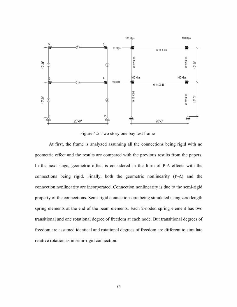
74
Figure 4.5 Two story one bay test frame
At first, the frame is analyzed assuming all the connections being rigid with no
geometric effect and the results are compared with the previous results from the papers.
In the next stage, geometric effect is considered in the form of P-Δ effects with the
connections being rigid. Finally, both the geometric nonlinearity (P-Δ) and the
connection nonlinearity are incorporated. Connection nonlinearity is due to the semi-rigid
property of the connections. Semi-rigid connections are being simulated using zero length
spring elements at the end of the beam elements. Each 2-noded spring element has two
transitional and one rotational degree of freedom at each node. But transitional degrees of
freedom are assumed identical and rotational degrees of freedom are different to simulate
relative rotation as in semi-rigid connection.

75
For moment-rotation curve, a bilinear elastic plastic moment-rotation curve has
been used. The moment-rotation curves used by King and Chen (1993) and Bhatti and
Hingtgen (1995) are shown in Figure 4.6. Present study follows the M-φ relationship
used by Bhatti and Hingtgen (1995), where they assumed initial stiffness for elastic
region with a value of 786732 kip-in/rad and Yield moment as 1989 kip-in.
Figure 4.6 Moment-Rotation relation used in previous study (Bhatti and Hingtgen,1995)
Lateral displacements at node 3 and 5, and absolute bending moments of all the elements
are tabulated in Table 4.2 and 4.3 for comparison.
Table 4.2 Lateral displacement (inch) for 2-Story test frame
Rigid without P- Δ Rigid with P- Δ Semi-rigid with P- Δ
Node #3 Node#5 Node #3 Node #5 Node #3 Node #5
Bhatti & Hingtgen 1.011 1.509 1.168 1.731 1.477 2.292
King & Chen - - 1.16 1.82 2.02 3.26
This Study 1.01184 1.51099 1.1623 1.72528 1.47056 2.28543

76
Table 4.3 Absolute Maximum Bending Moment (kip-inch) for 2-Story test frame
Element # 1 2 3 4 5 6
Rigid without P- Δ
Bhatti & Hingtgen 1450 711 1443 1437 711 711
King & Chen - - - - - - This Study 1449 711 1443 1437 711 711
Rigid with P- Δ
Bhatti & Hingtgen 1654 795 1677 1669 794 795
King & Chen 1649 794 1670 1664 794 794 This Study 1653 796 1675 1669 796 796
Semi-rigid with P- Δ
Bhatti & Hingtgen 1634 902 1739 1731 902 902
King & Chen 1560 1116 1837 1834 1116 1116 This Study 1633 903 1736 1731 903 903
The data presented in Table 4.2 and 4.3 verifies that the output from Opensees is
reliable based on the previous results. The results from the present study are much closer
with the results from Bhatti and Hingtgen (1995), as in both the cases moment-rotation
relation is similar which is a bilinear elastic plastic curve, while King and Chen (1993)
had used a different moment-rotation relation which may cause some difference.
4.4 20-Story Rectangular Hybrid Frame
Initially, a 20story frame has been modeled in Opensees software with SAC 20-
Story building dimensions. This 20-Story 5 bay frame is used in this study to observe the
effect of earthquake on high-rise buildings. The rectangular frame is 100 ft wide with 20
ft bay dimension, and the total height of the building is 289ft with two basement floor,
12ft each. All the member sizes are W24 X 131. Total dead load and 25 percentages of
live loads are considered for calculating effective seismic load. Load calculations are

77
described in Appendix G. At first, all the connections are considered to be rigid. Later,
partially restrained connections are incorporated in the structure to see the effect of semi-
rigid connections in the hybrid frames. All beam-to-column connections from level-7 to
11 are modeled as partially restrained. This configuration is selected based on the
previous study by Dobrinka Radulova (2009). The semi-rigid connections are
incorporated in the model by using a zero length spring element at the ends of the beam
members as shown in figure 4.3. Then, the semi-rigid connection property is assigned to
this spring element. Three different semi-rigid connections as per Table 4.1 have been
used. 20-story rectangular hybrid frame is shown in Figure 4.7. One rigid and three 20-
story hybrid rectangular frames are analyzed under five different earthquake excitation
records. Performance of the hybrid rectangular frame is compared with the rigid
rectangular frame and rigid rhombus frame.

78
Figure 4.7 Hybrid Rectangular: 20S – 289_100_2.89 – (RCSR) – E(7-11)

79
4.5 20-Story Rhombus Hybrid Frame
The 20-Story base rhombus frame has been modeled in Opensees software as
discussed in section 3.5. This frame is used in this study to observe the effect of semi-
rigid connections on rhombus shape buildings. To see the effect of height-to-width ratio
on the performance of the high rise structure, total width of this building is increased to
300ft. From 5, bay number increases to 15; Total Height and individual bay width remain
same. All the member sizes are W24 X 131. At the beginning all the connections are
considered to be rigid. Then, partially restrained connections are used on all the beam
ends from levels 7 though 11. The semi-rigid connections are introduced as a zero length
spring element following the previous section 4.4. Three different semi-rigid connections
as per Table 4.1 have been used. 20-story rhombus hybrid frames are shown in Figure 4.8
and 4.9. Two rigid and six 20-story hybrid rhombus frames are analyzed under five
different earthquake excitation records.

80
Figure 4.8 Hybrid Rhombus: 20S – 289_100_2.89 – (RMSR) – E(7-11)

81
Figure 4.9 Fat Hybrid Rhombus: 20S – 289_300_0.963 – (RMSR) – E(7-11)

82
4.6 Discussion of the Results
In this chapter, hybrid frames are compared with the corresponding rigid frames.
Then, the rectangular hybrid frame is compared with the rigid rhombus frame. Hybrid
rectangular frames show improved performance than the rectangular rigid frame in most
of the cases. Top node displacements for rectangular rigid and hybrid frames are shown
in Figure A.21 through A.25. Maximum displacements for each story are plotted from
Figure E.21 through E.25. Figure 4.10 shows the displacement profile for 20S –
289_100_2.89–(RCR, RCSR)–E1m (7-11) frames. It shows, for ElCentro, Northridge
and Parkfield earthquakes, maximum lateral sway decreased for hybrid rectangular frame
comparing to the rigid rectangular frame. But hybrid frame gives more lateral
displacement than rigid frame when subjected to the Kocaeli earthquakes.
-2-10123456789
101112131415161718192021
0 8 16 24 32 40Maximum Displacement, Ux (inch)
Stor
y
-18.4 1.6 21.6 41.6 61.6 81.6 101.6Maximum Displacement, Ux(cm)
Parkfield, rigidElCentro, rigidNorthridge, rigidKocaeli-1, rigidKocaeli-2,rigidParkfield, semi-rigidElCentro, semi-rigidNorthridge, semi-rigidKocaeli-1, semi-rigidKocaeli-2, semi-rigid
20S-289_100_2.89-MDux-E1m(7-11)
Figure 4.10 Maximum lateral sway 20S-289_100_2.89–MDUx (RCR,RCSR)–E1m(7-11)

83
This can be explained by comparing the frequency of the frame with the
earthquake frequencies. Earthquake frequencies are tabulated in chapter 3 from Table 3.5
through 3.10. Hybrid and rigid frame frequencies obtained from the Opensees software
are tabulated in Table 4.4.
Table 4.4 Rectangular rigid and hybrid frame frequencies (Opensees)
Mode 20S –289_100_2.89–RCR 20S-289_100_2.89-RCSR-E1m (7-11) (Hz) (Hz)
1 0.3962 0.34146 2 1.24918 1.18438 3 2.24456 1.89239 4 3.21852 2.85043 5 4.24537 3.92719 6 5.30505 4.73884 7 6.42361 5.98415 8 7.58788 7.08584 9 8.80896 8.24295
10 10.0716 9.56393
First two mode frequencies for the hybrid frame are much closer to the first two
dominant frequencies for Afyon Bay and Aydin records for Kocaeli earthquake. This
causes resonance effect for hybrid frame when subjected to Kocaeli earthquake. Earlier it
was defined that, ElCentro and Northridge are high frequency, and Parkfield is a medium
frequency earthquakes. High rise structures have low frequencies, and semi-rigid
connections reduce it more. So, high and medium frequency earthquakes do not create
resonance effect on hybrid rectangular frames unless the original rigid structure is too
stiff.

84
Inter story lateral drifts for rigid and hybrid rectangular frames are plotted in
Figure F.21 through F.25. Figure 4.11 shows the inter story drift profile for hybrid and
rigid rectangular frame for one type of semi rigid connections. For Northridge
earthquake, hybrid frame experience less drift than the rigid frame. Hybrid frame
subjected to ElCentro and Parkfield earthquake gives greater drift values in the mid levels
of the structure than the rigid rectangular frame. These increases in the lateral drift in
hybrid frame are due to the placing of semi-rigid connections at the mid levels of the
structure. Semi-rigid connections make a structure flexible and for that reason, in those
levels the structure experience more drifts than the rigid frame. Both records from
Kocaeli earthquake gives more drift values in hybrid frame than the rigid rectangular
frame due to resonance effect discussed before.
-2-10123456789
101112131415161718192021
0 0.005 0.01 0.015 0.02Lateral Drift
Sto
ry
Parkfield, rigidElCentro, rigidNorthridge, rigidKocaeli-1, rigidKocaeli-2,rigidParkfield, semi-rigidElCentro, semi-rigidNorthridge, semi-rigidKocaeli-1, semi-rigidKocaeli-2, semi-rigid
20S-289_100_2.89-LDr-E1m(7-11)Life Safety limit 0.025Collapse Prevention limit 0.05
Figure 4.11 20S – 289_100_2.89–LDr (RCR,RCSR) –E1m(7-11)

85
Internal forces are also compared between hybrid and rigid rectangular frames. In
most of the cases, hybrid frames perform better than the rigid frames, when subjected to
high and medium frequency earthquakes. But hybrid frames do not perform as expected,
under low frequency Kocaeli earthquake. This is due to the resonance effect. Figure 4.12
shows the beam bending moment ratios from hybrid and rigid rectangular frame.
-2-10123456789
101112131415161718192021
0 1 2 3Bending Moment ratio
Sto
ry
Data for ParkfieldData for ElCentroData for NorthridgeData for Kocaeli-1Data for Kocaeli-2
20S-289_100_2.89-BM(RCSR/RCR)-E1m(7-11)
Figure 4.12 20S – 289_100_2.89 – BM (RCSR/RCR) – E1m(7-11) for Beams
Shear force and bending moment ratios in Figure C.21 thorough C.25 and D.21
through D.25 shows the similar pattern. Except low frequency Kocaeli earthquake, in
most of the cases hybrid frames demand less forces than the rigid frames. The beam
bending moment demand reduces 11 times lower than the demand from rigid rectangular
frame. None of the beams in ElCentro and Northridge earthquake demand more beam
bending force than the rigid rectangular frame. The maximum increase in beam bending
moment demand is 2 times higher than the rigid frame for Aydin record of Kocaeli

86
earthquake. Maximum column moment demand increase in hybrid frames is 2.5 times
higher than the rigid rectangular frame.
Axial force ratios between hybrid and rigid rectangular frames are shown through
Figure B.21 through B.25. Axial force demand for hybrid frames increase at the mid level
due to the placing of semi-rigid connections at these locations. Maximum increase in
beam axial force is 108 times higher than the rigid frame when subjected to Aydin record
of Kocaeli earthquake. And maximum decrease in demand is 26 times lower than the
rigid frame for Northridge earthquake. In most of the cases axial force demand is less for
hybrid rectangular frames. Only demand increase when subjected to Kocaeli records.
Highest increase is 50 percent than the rigid frame. Maximum decrease in column axial
force demand is 7 times lower than the rigid rectangular frame for Northridge earthquake.
Hybrid rhombus frame is also compared with the rigid rhombus frame. But the
effect of semi-rigid connections in the rhombus frame is not that much significant as
observed in case of rectangular frame. Frequency of rigid and hybrid frames are almost
equal. Frequencies obtained for hybrid and rigid rhombus frame modeled in Opensees
software is tabulated in table 4.5.

87
Table 4.5 Rhombus rigid and hybrid frame frequencies (Opensees)
Mode 20S –289_100_2.89–RMR 20S-289_100_2.89-RMSR-E1m (7-11)
(Hz) (Hz) 1 0.64306 0.63469 2 2.251356 1.728858 3 3.985531 3.653391 4 4.878337 4.468481 5 6.906455 6.060516 6 7.946315 7.009683 7 9.560905 8.739879 8 10.88132 9.966534 9 12.51924 11.65015
10 14.31197 13.53017
Semi-rigid connections can not provide expected flexibility to the hybrid rhombus
frame. As, both of the hybrid and rigid frame bear almost same frequency, Figure A.26 to
A.30 and E.26 to E.30 shows top node displacement and sway profile which do not
significantly varies for hybrid rhombus frames than the rigid rhombus frames. Figure
4.13 shows the lateral sway for 20S –289_100_2.89–(RMR, RMSR)–E1m (7-11) frames.
Figure F.26 through F.30 show, that the frame has more lateral drift in the mid levels for
hybrid frames than the rigid rhombus frame, as semi-rigid connections are placed in those
places. On the other levels with rigid connections, hybrid rhombus frame demand less
lateral drift than the rigid rhombus frame. Figure 4.14 shows inter story drifts for 20S –
289_100_2.89–(RMR, RMSR)–E1m (7-11) frames.

88
-2-10123456789
101112131415161718192021
0 4 8 12 16 20Maximum Displacement, Ux (inch)
Stor
y0 10 20 30 40 50
Maximum Displacement, Ux(cm)
Parkfield, rigidElCentro, rigidNorthridge, rigidKocaeli-1, rigidKocaeli-2,rigidParkfield, semi-rigidElCentro, semi-rigidNorthridge, semi-rigidKocaeli-1, semi-rigidKocaeli-2, semi-rigid
Figure 4.13 Maximum lateral sway 20S-289_100_2.89-MDUx(RMR,RMSR)-E1m(7-11)
-2-10123456789
101112131415161718192021
0 0.005 0.01 0.015Lateral Drift
Sto
rey
Parkfield, rigidElCentro, rigidNorthridge, rigidKocaeli-1, rigidKocaeli-2,rigidParkfield, semi-rigidElCentro, semi-rigidNorthridge, semi-rigidKocaeli-1, semi-rigidKocaeli-2, semi-rigid
20S-289_100_2.89-LDr(RMR,RMSR)-E1m(7-11)Life Safety limit 0.025Collapse Prevention limit 0.05
Figure 4.14 20S –289_100_2.89–LDr (RMR,RMSR)–E1m(7-11)

89
Hybrid rhombus frame does not show better redistribution pattern of internal
forces as hybrid rectangular frame has shown previously. Placing of semi-rigid
connections at the mid levels scattered points at that level for internal force ratios
between hybrid and rigid rhombus frames. Below and upper level of frame does not
experience significant change in demand for hybrid rhombus frame than the rigid
rhombus frame. Figure 4.15 shows the beam bending moment ratio between hybrid and
rigid frames.
-2-10123456789
101112131415161718192021
0 1 2 3Bending Moment ratio
Stor
y
Data for ParkfieldData for ElCentroData for NorthridgeData for Kocaeli-1Data for Kocaeli-2
20S-289_100_2.89-BM(RCSR/RCR)-E1m(7-11)
Figure 4.15 20S – 289_100_2.89 – BM (RMSR/RMR) – E1m(7-11) for Beams
With the usage of stiffer semi-rigid connections, the internal force ratios move to
near 1. These are shown in figure B.26 to B.30, C.26 to C.30 and D.26 to D.30.
Maximum column axial force demand for hybrid rhombus frame is around 7 times higher
and minimum is 5 times lower than the rigid rhombus frame demand for Aydin record of

90
Kocaeli earthquake. Maximum beam shear demand is 192 percent higher and minimum
demand is 138 percent lower for hybrid rhombus frame than rigid rhombus frame for
Aydin record of Kocaeli earthquake. Hybrid rhombus frame demand maximum 185
percent higher moment than the rigid rhombus frame subjected to Parkfield earthquake,
and minimum beam moment demand is 138 percent lower for hybrid rhombus frame than
the rigid rhombus frame.
Internal forces for the rigid rhombus frames are compared to the hybrid
rectangular frames. Ratios of axial force demand between rigid rhombus frame and
hybrid rectangular frame are shown in figure B.31 to B.35. In most of the cases, rigid
rhombus frame demands more column axial force, than the hybrid rectangular frame. The
maximum demand of column axial force for the rigid rhombus frame is 5.5 times higher
than the demand for hybrid rectangular frame, subjected to Parkfield earthquake. The
column axial force demands on the top floors for rigid rhombus frame are significantly
lower than the hybrid rectangular frame. The minimum demand for column axial force
for rigid rhombus frame is 26 times lower than the hybrid rectangular frame for Aydin
record of Kocaeli earthquake.
Figure C.31 to C.35 and D.31 to D.35 shows the shear force and bending moment
ratios between rigid rhombus frame and hybrid rectangular frame. Rigid rhombus frame
improves building performance for low earthquake records. And the minimum bending
moment required by rigid rhombus frame is 71 times lower for column, and 24 times

91
lower for beam, than the hybrid rectangular frame, for Aydin record of Kocaeli
earthquake. Most of the beams and columns below mid level of the rigid rhombus frame,
demand more shear force and bending moment than the hybrid rectangular frame
subjected to medium and high frequency earthquakes. The maximum beam bending
moment demand for rigid rhombus frame is 3.4 times higher than the hybrid rectangular
frame bending demand, for Parkfield earthquake. Top floors above mid levels of rigid
rhombus frame demand less shear and bending moment for column and beams. Minimum
bending moment demand for rigid rhombus frame is around 12 times lower than the
demand for hybrid rectangular frame for ElCentro earthquake.
Figures B.36 to B.40, C.36 to C.40 and D.36 to D.40 show the axial force, shear
force and bending moment ratios between fat hybrid rhombus frame with the fat rigid
rhombus frame. This frames are designated by 20S –289_300_0.963–(RMR, RMSR)–(7-
11). Results from this frames show scattered point in the mid levels where semi rigid
connections are placed. On the other levels, these internal force ratios move close to one.

92
CHAPTER 5
CONCLUSIONS AND RECOMMENDATIONS
5.1 Summary
The primary objective of this study is to present an efficient building geometric
shape for earthquake force resisting frame system. A rhombus shape is created from the
popular rectangular moment frame for this purpose. In the first stage, several rhombus
frames have been constructed to cover from low-rise to high-rise buildings. Then, these
frames are analyzed under five earthquake records with wide frequency contents. The
results are compared with the rectangular frames with the same geometric aspect ratios.
Then, different semi-rigid connection properties are introduced in the high rise rhombus
and rectangular frames. Behaviors of hybrid frames with both rigid and semi-rigid
connections, when subjected to earthquake excitations, are closely observed, and results
are compared with their equivalent rigid frames. The width of the high rise rhombus
frame is increased to observe the effect on seismic performance. This fat rhombus frame
is also compared with its equivalent hybrid frames. In the last stage, the rigid rhombus
frame is compared with the hybrid rectangular frame.

93
5.2 Conclusions
Comparing four rigid rhombus frames to four rigid rectangular frames under five
earthquake records, the rhombus frames performed better than the rectangular frames.
Introducing semi-rigid connections in the high-rise structures, the hybrid rectangular
frame with rigid and semi-rigid connections showed improved performance over the rigid
rectangular frame. Comparing the hybrid rectangular frame to the rigid rhombus frame,
the major conclusions drawn from this study are summarized below –
Rigid rhombus frames are much stiffer than the rigid rectangular frames.
Top node displacements and lateral sway values from the 3-, 9-, 12- and 20-story
rigid rhombus frames are less than that of the equivalent rigid rectangular frames.
For all the considered earthquakes, 3-, 9- and 12- story rigid rhombus frames
experience less inter story drift than the rectangular rigid frames. But, few stories
of a 20-story rigid rhombus frame experience a little more drift than the rigid
rectangular frame for Parkfield and Afyon Bay records for Kocaeli earthquakes.
In most of the cases, rigid rhombus frames demand less shear force and bending
moment than the rigid rectangular frames.
In few cases, bottom stories of 20-story rigid rhombus frame demand more shear
force and bending moment than the rigid rectangular frame. But, this is negligible
comparing to the reduction of demand in other stories.
Rigid rhombus frames demand more axial force than the rigid rectangular frames.
This is true for both the beams and columns. Beams in the middle portion of the
rigid rhombus frames demand maximum axial force in most of the cases.

94
Semi-rigid connections increase the flexibility of the frames, and thus reduce the
frequency of the structure. Semi-rigid connections have significant influence on
reducing the frequency of rectangular frames; but they do not have a significant
effect on rhombus frames.
20-story rectangular hybrid frames with semi-rigid connections in the mid levels
exhibited improve building performance over the equivalent rigid rectangular
frame, when subjected to medium and high frequency earthquakes. Due to
reduction of frame frequency, by use of semi-rigid connection the probability of
resonance in high and medium frequency earthquakes is lowered. This results in
less internal forces demand. But for low frequency earthquakes, high rise
rectangular frames with semi-rigid connections are good candidates to produce
resonance.
Hybrid rectangular frames exhibit more lateral drift in the stories where semi-
rigid connections are placed. Sometimes this condition could result in a soft story
mechanism. Experienced judgment is required for placing semi-rigid connections
in rectangular frames.
The location pattern used in this study for semi-rigid connections does not have
much effect on the rhombus shape hybrid frame. Frame frequency reduces
slightly. The frame does show some flexibility on the stories, where semi-rigid
connections are placed, but the effect on the global behavior of the frame is
insignificant.
95
A fat hybrid rhombus frame behaves in the same way as a base hybrid rhombus
frame.
Redistribution of internal forces depends on the semi-rigid connection property.
Hybrid frames with relatively stiffer semi-rigid connections, demand internal
forces almost same as that for rigid frames.
High rise rigid rhombus frames perform better than the high rise hybrid
rectangular frames in low frequency earthquakes.
5.3 Recommendations
As this study attempts to propose a new earthquake resistance framing system, the
following recommendations for future work are made –
Semi-rigid connections need to be applied at different locations in the rhombus
frames to observe the seismic performance. Here in this study, semi-rigid
connections are placed only on the mid stories. Different pattern of placing semi-
rigid connections may significantly modify the results for rhombus shape.
Modifications in the frame assembly can be tried to reduce the axial force
demand in Rhombus frame.
Comparisons to be made with other bracing systems such as concentrically
braced frame and eccentrically braced frame.

96
APPENDIX A
TOP LATERAL DISPLACEMENT

97
-8
-6
-4
-2
0
2
4
6
8
0 5 10 15 20 25 30 35 40Time(sec)
Dis
plac
emen
t-Ux(
inch
)
-20.32
-16.32
-12.32
-8.32
-4.32
-0.32
3.68
7.68
11.68
15.68
19.68
Dis
plac
emen
t-Ux(
cm)
3S-39_120_0.325-TDUx(RMR)-PKF 3S-39_120_0.325-TDUx(RCR)-PKF
Figure A.1 Top lateral displacement for 3S-39_120_0.325-PKF
-4
-3
-2
-1
0
1
2
3
4
0 5 10 15 20 25 30Time(sec)
Dis
plac
emen
t-Ux(
inch
)
-10.16
-7.66
-5.16
-2.66
-0.16
2.34
4.84
7.34
9.84
Dis
plac
emen
t-Ux(
cm)
3S-39_120_0.325-TDUx(RMR)-ELC 3S-39_120_0.325-TDUx(RCR)-ELC
Figure A.2 Top lateral displacement for 3S-39_120_0.325-ELC

98
-5
-4
-3
-2
-1
0
1
2
3
4
5
0 10 20 30 40 50Time(sec)
Dis
plac
emen
t-Ux(
inch
)
-12.7
-10.2
-7.7
-5.2
-2.7
-0.2
2.3
4.8
7.3
9.8
12.3
Dis
plac
emen
t-Ux(
cm)
3S-39_120_0.325-TDUx(RMR)-NRG 3S-39_120_0.325-TDUx(RCR)-NRG
Figure A.3 Top lateral displacement for 3S-39_120_0.325-NRG
-0.15
-0.1
-0.05
0
0.05
0.1
0.15
0 30 60 90 120 150 180Time(sec)
Dis
plac
emen
t-Ux(
inch
)
-0.381
-0.301
-0.221
-0.141
-0.061
0.019
0.099
0.179
0.259
0.339
Dis
plac
emen
t-Ux(
cm)
3S-39_120_0.325-TDUx(RMR)-KCL1 3S-39_120_0.325-TDUx(RCR)-KCL1
Figure A.4 Top lateral displacement for 3S-39_120_0.325-KCL1

99
-0.05
-0.04
-0.03
-0.02
-0.01
0
0.01
0.02
0.03
0.04
0.05
0 30 60 90 120 150 180 210Time(sec)
Dis
plac
emen
t-Ux(
inch
)
-0.127
-0.102
-0.077
-0.052
-0.027
-0.002
0.023
0.048
0.073
0.098
0.123
Dis
plac
emen
t-Ux(
cm)
3S-39_120_0.325-TDUx(RMR)-KCL2 3S-39_120_0.325-TDUx(RCR)-KCL2
Figure A.5 Top lateral displacement for 3S-39_120_0.325-KCL2
-20
-15
-10
-5
0
5
10
15
20
0 5 10 15 20 25 30 35 40Time(sec)
Dis
plac
emen
t-Ux(
inch
)
-50.8
-40.8
-30.8
-20.8
-10.8
-0.8
9.2
19.2
29.2
39.2
49.2
Dis
plac
emen
t-Ux(
cm)
9S-134_150_0.893-TDUx(RMR)-PKF 9S-134_150_0.893-TDUx(RCR)-PKF
Figure A.6 Top lateral displacement for 9S-134_150_0.893-PKF

100
-10
-8
-6
-4
-2
0
2
4
6
8
10
0 5 10 15 20 25 30Time(sec)
Dis
plac
emen
t-Ux(
inch
)
-25.4
-20.4
-15.4
-10.4
-5.4
-0.4
4.6
9.6
14.6
19.6
24.6
Dis
plac
emen
t-Ux(
cm)
9S-134_150_0.893-TDUx(RMR)-ELC 9S-134_150_0.893-TDUx(RCR)-ELC
Figure A.7 Top lateral displacement for 9S-134_150_0.893-ELC
-25
-20
-15
-10
-5
0
5
10
15
20
25
0 10 20 30 40 50Time(sec)
Dis
plac
emen
t-Ux(
inch
)
-63.5
-53.5
-43.5
-33.5
-23.5
-13.5
-3.5
6.5
16.5
26.5
36.5
46.5
56.5
Dis
plac
emen
t-Ux(
cm)
9S-134_150_0.893-TDUx(RMR)-NRG 9S-134_150_0.893-TDUx(RCR)-NRG
Figure A.8 Top lateral displacement for 9S-134_150_0.893-NRG

101
-0.6
-0.4
-0.2
0
0.2
0.4
0.6
0 30 60 90 120 150 180Time(sec)
Dis
plac
emen
t-Ux(
inch
)
-1.524
-1.224
-0.924
-0.624
-0.324
-0.024
0.276
0.576
0.876
1.176
1.476
Dis
plac
emen
t-Ux(
cm)
9S-134_150_0.893-TDUx(RMR)-KCL1 9S-134_150_0.893-TDUx(RCR)-KCL1
Figure A.9 Top lateral displacement for 9S-134_150_0.893-KCL1
-1
-0.8
-0.6
-0.4
-0.2
0
0.2
0.4
0.6
0.8
1
0 30 60 90 120 150 180 210Time(sec)
Dis
plac
emen
t-Ux(
inch
)
-2.54
-2.04
-1.54
-1.04
-0.54
-0.04
0.46
0.96
1.46
1.96
2.46
Dis
plac
emen
t-Ux(
cm)
9S-134_150_0.893-TDUx(RMR)-KCL2 9S-134_150_0.893-TDUx(RCR)-KCL2
Figure A.10 Top lateral displacement for 9S-134_150_0.893-KCL2

102
-20
-15
-10
-5
0
5
10
15
20
0 5 10 15 20 25 30 35 40Time(sec)
Dis
plac
emen
t-Ux(
inch
)
-50.8
-40.8
-30.8
-20.8
-10.8
-0.8
9.2
19.2
29.2
39.2
49.2
Dis
plac
emen
t-Ux(
cm)
12S-173_150_1.153-TDUx(RMR)-PKF 12S-173_150_1.153-TDUx(RCR)-PKF
Figure A.11 Top lateral displacement for 12S-173_150_1.153-PKF
-20
-15
-10
-5
0
5
10
15
20
0 5 10 15 20 25 30Time(sec)
Dis
plac
emen
t-Ux(
inch
)
-50.8
-40.8
-30.8
-20.8
-10.8
-0.8
9.2
19.2
29.2
39.2
49.2
Dis
plac
emen
t-Ux(
cm)
12S-173_150_1.153-TDUx(RMR)-ELC 12S-173_150_1.153-TDUx(RCR)-ELC
Figure A.12 Top lateral displacement for 12S-173_150_1.153-ELC

103
-40
-30
-20
-10
0
10
20
30
40
0 10 20 30 40 50Time(sec)
Dis
plac
emen
t-Ux(
inch
)
-101.6
-81.6
-61.6
-41.6
-21.6
-1.6
18.4
38.4
58.4
78.4
98.4
Dis
plac
emen
t-Ux(
cm)
12S-173_150_1.153-TDUx(RMR)-NRG 12S-173_150_1.153-TDUx(RCR)-NRG
Figure A.13 Top lateral displacement for 12S-173_150_1.153-NRG
-1
-0.8
-0.6
-0.4
-0.2
0
0.2
0.4
0.6
0.8
1
0 30 60 90 120 150 180Time(sec)
Dis
plac
emen
t-Ux(
inch
)
-2.54
-2.04
-1.54
-1.04
-0.54
-0.04
0.46
0.96
1.46
1.96
2.46
Dis
plac
emen
t-Ux(
cm)
12S-173_150_1.153-TDUx(RMR)-KCL1 12S-173_150_1.153-TDUx(RCR)-KCL1
Figure A.14 Top lateral displacement for 12S-173_150_1.153-KCL1

104
-1.5
-1.2
-0.9
-0.6
-0.3
0
0.3
0.6
0.9
1.2
1.5
0 30 60 90 120 150 180 210Time(sec)
Dis
plac
emen
t-Ux(
inch
)
-3.81
-3.01
-2.21
-1.41
-0.61
0.19
0.99
1.79
2.59
3.39
Dis
plac
emen
t-Ux(
cm)
12S-173_150_1.153-TDUx(RMR)-KCL2 12S-173_150_1.153-TDUx(RCR)-KCL2
Figure A.15 Top lateral displacement for 12S-173_150_1.153-KCL2
-25
-20
-15
-10
-5
0
5
10
15
20
25
0 5 10 15 20 25 30 35 40Time(sec)
Dis
plac
emen
t-Ux(
inch
)
-63.5
-53.5
-43.5
-33.5
-23.5
-13.5
-3.5
6.5
16.5
26.5
36.5
46.5
56.5
Dis
plac
emen
t-Ux(
cm)
20S-289_100_2.89-TDUx(RMR)-PKF 20S-289_100_2.89-TDUx(RCR)-PKF
Figure A.16 Top lateral displacement for 20S-289_100_2.89-PKF

105
-20
-15
-10
-5
0
5
10
15
20
0 5 10 15 20 25 30Time(sec)
Dis
plac
emen
t-Ux(
inch
)
-50.8
-40.8
-30.8
-20.8
-10.8
-0.8
9.2
19.2
29.2
39.2
49.2
Dis
plac
emen
t-Ux(
cm)
20S-289_100_2.89-TDUx(RMR)-ELC 20S-289_100_2.89-TDUx(RCR)-ELC
Figure A.17 Top lateral displacement for 20S-289_100_2.89-ELC
-40
-30
-20
-10
0
10
20
30
40
0 10 20 30 40 50Time(sec)
Dis
plac
emen
t-Ux(
inch
)
-101.6
-81.6
-61.6
-41.6
-21.6
-1.6
18.4
38.4
58.4
78.4
98.4
Dis
plac
emen
t-Ux(
cm)
20S-289_100_2.89-TDUx(RMR)-NRG 20S-289_100_2.89-TDUx(RCR)-NRG
Figure A.18 Top lateral displacement for 20S-289_100_2.89-NRG

106
-1
-0.8
-0.6
-0.4
-0.2
0
0.2
0.4
0.6
0.8
1
0 30 60 90 120 150 180Time(sec)
Dis
plac
emen
t-Ux(
inch
)
-2.54
-2.04
-1.54
-1.04
-0.54
-0.04
0.46
0.96
1.46
1.96
2.46
Dis
plac
emen
t-Ux(
cm)
20S-289_100_2.89-TDUx(RMR)-KCL1 20S-289_100_2.89-TDUx(RCR)-KCL1
Figure A.19 Top lateral displacement for 20S-289_100_2.89-KCL1
-1.75
-1.45
-1.15
-0.85
-0.55
-0.25
0.05
0.35
0.65
0.95
1.25
1.55
0 30 60 90 120 150 180 210Time(sec)
Dis
plac
emen
t-Ux(
inch
)
-4.445
-3.645
-2.845
-2.045
-1.245
-0.445
0.355
1.155
1.955
2.755
3.555
4.355
Dis
plac
emen
t-Ux(
cm)
20S-289_100_2.89-TDUx(RMR)-KCL2 20S-289_100_2.89-TDUx(RCR)-KCL2
Figure A.20 Top lateral displacement for 20S-289_100_2.89-KCL2

107
-25
-20
-15
-10
-5
0
5
10
15
20
25
0 5 10 15 20 25 30 35 40
Time(sec)
Dis
plac
emen
t-Ux(
inch
)
-63.5
-53.5
-43.5
-33.5
-23.5
-13.5
-3.5
6.5
16.5
26.5
36.5
46.5
56.5
Dis
plac
emen
t-Ux(
cm)
RigidSemi-rigid, E=1millionSemi-rigid, E=3millionSemi-rigid, E=5million
20S-289_100_2.89-TDux-PKF-E(7-11)
Figure A.21 Top lateral displacement for 20S-289_100_2.89-PKF
-25
-20
-15
-10
-5
0
5
10
15
20
25
0 5 10 15 20 25 30
Time(sec)
Dis
plac
emen
t-Ux(
inch
)
-63.5
-53.5
-43.5
-33.5
-23.5
-13.5
-3.5
6.5
16.5
26.5
36.5
46.5
56.5
Dis
plac
emen
t-Ux(
cm)
RigidSemi-rigid, E=1millionSemi-rigid, E=3millionSemi-rigid, E=5million
20S-289_100_2.89-TDux-ELC-E(7-11)
Figure A.22 Top lateral displacement for 20S-289_100_2.89-ELC

108
-50
-40
-30
-20
-10
0
10
20
30
40
50
0 10 20 30 40 50
Time(sec)
Dis
plac
emen
t-Ux(
inch
)
-127
-107
-87
-67
-47
-27
-7
13
33
53
73
93
113
Dis
plac
emen
t-Ux(
cm)
RigidSemi-rigid, E=1millionSemi-rigid, E=3millionSemi-rigid, E=5million
20S-289_100_2.89-TDux-NRG-E(7-11)
Figure A.23 Top lateral displacement for 20S-289_100_2.89-NRG
-1.5
-1.2
-0.9
-0.6
-0.3
0
0.3
0.6
0.9
1.2
1.5
0 36 72 108 144 180
Time(sec)
Dis
plac
emen
t-Ux(
inch
)
-3.81
-3.01
-2.21
-1.41
-0.61
0.19
0.99
1.79
2.59
3.39
Dis
plac
emen
t-Ux(
cm)
RigidSemi-rigid, E=1millionSemi-rigid, E=3millionSemi-rigid, E=5million
20S-289_100_2.89-TDux-KCL1-E(7-11)
Figure A.24 Top lateral displacement for 20S-289_100_2.89-KCL1

109
-1.75
-1.5
-1.25
-1
-0.75
-0.5
-0.25
0
0.25
0.5
0.75
1
1.25
1.5
1.75
0 40 80 120 160 200
Time(sec)
Dis
plac
emen
t-Ux(
inch
)
-4.445
-3.545
-2.645
-1.745
-0.845
0.055
0.955
1.855
2.755
3.655
Dis
plac
emen
t-Ux(
cm)
RigidSemi-rigid, E=1millionSemi-rigid, E=3millionSemi-rigid, E=5million
20S-289_100_2.89-TDux-KCL2-E(7-11)
Figure A.25 Top lateral displacement for 20S-289_100_2.89-KCL2
-20
-15
-10
-5
0
5
10
15
20
0 5 10 15 20 25 30 35 40
Time(sec)
Dis
plac
emen
t-Ux(
inch
)
-50.8
-40.8
-30.8
-20.8
-10.8
-0.8
9.2
19.2
29.2
39.2
49.2
Dis
plac
emen
t-Ux(
cm)
RigidSemi-rigid, E=1millionSemi-rigid, E=3millionSemi-rigid, E=5million
20S-289_100_2.89-TDux-PKF-E(7-11)
Figure A.26 Top lateral displacement for 20S-289_100_2.89-PKF

110
-10
-8
-6
-4
-2
0
2
4
6
8
10
0 5 10 15 20 25 30
Time(sec)
Dis
plac
emen
t-Ux(
inch
)
-63.5
-53.5
-43.5
-33.5
-23.5
-13.5
-3.5
6.5
16.5
26.5
36.5
46.5
56.5
Dis
plac
emen
t-Ux(
cm)
RigidSemi-rigid, E=1millionSemi-rigid, E=3millionSemi-rigid, E=5million
20S-289_100_2.89-TDux-ELC-E(7-11)
Figure A.27 Top lateral displacement for 20S-289_100_2.89-ELC
-20
-15
-10
-5
0
5
10
15
20
0 10 20 30 40 50
Time(sec)
Dis
plac
emen
t-Ux(
inch
)
-50.8
-40.8
-30.8
-20.8
-10.8
-0.8
9.2
19.2
29.2
39.2
49.2
Dis
plac
emen
t-Ux(
cm)
RigidSemi-rigid, E=1millionSemi-rigid, E=3millionSemi-rigid, E=5million
20S-289_100_2.89-TDux-NRG-E(7-11)
Figure A.28 Top lateral displacement for 20S-289_100_2.89-NRG

111
-1
-0.8
-0.6
-0.4
-0.2
0
0.2
0.4
0.6
0.8
1
0 30 60 90 120 150 180
Time(sec)
Dis
plac
emen
t-Ux(
inch
)
-2.54
-2.04
-1.54
-1.04
-0.54
-0.04
0.46
0.96
1.46
1.96
2.46
Dis
plac
emen
t-Ux(
cm)
RigidSemi-rigid, E=1millionSemi-rigid, E=3millionSemi-rigid, E=5million
20S-289_100_2.89-TDux-KCL1-E(7-11)
Figure A.29 Top lateral displacement for 20S-289_100_2.89-KCL1
-1
-0.8
-0.6
-0.4
-0.2
0
0.2
0.4
0.6
0.8
1
0 30 60 90 120 150 180 210
Time(sec)
Dis
plac
emen
t-Ux(
inch
)
-2.54
-2.04
-1.54
-1.04
-0.54
-0.04
0.46
0.96
1.46
1.96
2.46
Dis
plac
emen
t-Ux(
cm)
RigidSemi-rigid, E=1millionSemi-rigid, E=3millionSemi-rigid, E=5million
20S-289_100_2.89-TDux-KCL2-E(7-11)
Figure A.30 Top lateral displacement for 20S-289_100_2.89-KCL2

112
APPENDIX B
AXIAL FORCES IN THE FRAME ELEMENTS

113
0
1
2
3
0 1 2 3 4 5Axial Force ratio
Stor
y
Absolute AFmax ratio 3S-39_120_0.325-AF(RMR/RCR)-PKF
a)
0
1
2
3
4
0 1 2 3 4 5Axial Force ratio
Stor
y
Absolute AFmax ratio 3S-39_120_0.325-AF(RMR/RCR)-PKF
b)
Figure B.1 Axial Force ratio for 3S-39_120_0.325-PKF a)Beams, b)Columns
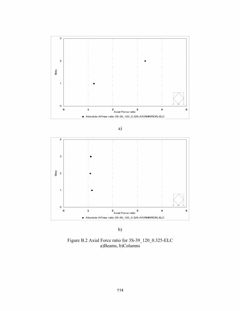
114
0
1
2
3
0 1 2 3 4 5Axial Force ratio
Stor
y
Absolute AFmax ratio 3S-39_120_0.325-AF(RMR/RCR)-ELC
a)
0
1
2
3
4
0 1 2 3 4 5Axial Force ratio
Stor
y
Absolute AFmax ratio 3S-39_120_0.325-AF(RMR/RCR)-ELC
b)
Figure B.2 Axial Force ratio for 3S-39_120_0.325-ELC a)Beams, b)Columns
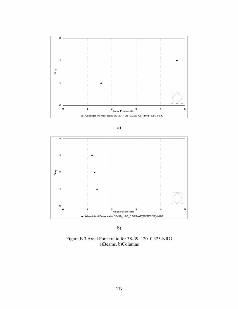
115
0
1
2
3
0 1 2 3 4 5Axial Force ratio
Stor
y
Absolute AFmax ratio 3S-39_120_0.325-AF(RMR/RCR)-NRG
a)
0
1
2
3
4
0 1 2 3 4 5Axial Force ratio
Stor
y
Absolute AFmax ratio 3S-39_120_0.325-AF(RMR/RCR)-NRG
b)
Figure B.3 Axial Force ratio for 3S-39_120_0.325-NRG a)Beams, b)Columns

116
0
1
2
3
0 1 2 3 4 5Axial Force ratio
Stor
y
Absolute AFmax ratio 3S-39_120_0.325-AF(RMR/RCR)-KCL1
a)
0
1
2
3
4
0 1 2 3 4 5Axial Force ratio
Stor
y
Absolute AFmax ratio 3S-39_120_0.325-AF(RMR/RCR)-KCL1
b)
Figure B.4 Axial Force ratio for 3S-39_120_0.325-KCL1 a)Beams, b)Columns

117
0
1
2
3
0 1 2 3 4 5Axial Force ratio
Stor
y
Absolute AFmax ratio 3S-39_120_0.325-AF(RMR/RCR)-KCL2
a)
0
1
2
3
4
0 1 2 3 4 5Axial Force ratio
Stor
y
Absolute AFmax ratio 3S-39_120_0.325-AF(RMR/RCR)-KCL2
b)
Figure B.5 Axial Force ratio for 3S-39_120_0.325-KCL2 a)Beams, b)Columns

118
0
1
2
3
4
5
6
7
8
9
0 20 40 60 80 100Axial Force ratio
Stor
y
Absolute AFmax ratio 9S-134_150_0.893-AF(RMR/RCR)-PKF
a)
0
1
2
3
4
5
6
7
8
9
10
0 1 2 3 4 5Axial Force ratio
Stor
y
Absolute AFmax ratio 9S-134_150_0.893-AF(RMR/RCR)-PKF
b)
Figure B.6 Axial Force ratio for 9S-134_150_0.893-PKF a)Beams, b)Columns

119
0
1
2
3
4
5
6
7
8
9
0 20 40 60 80 100Axial Force ratio
Stor
y
Absolute AFmax ratio 9S-134_150_0.893-AF(RMR/RCR)-ELC
a)
0
1
2
3
4
5
6
7
8
9
10
0 1 2 3 4 5Axial Force ratio
Stor
y
Absolute AFmax ratio 9S-134_150_0.893-AF(RMR/RCR)-ELC
b)
Figure B.7 Axial Force ratio for 9S-134_150_0.893-ELC a)Beams, b)Columns

120
0
1
2
3
4
5
6
7
8
9
0 20 40 60 80 100Axial Force ratio
Stor
y
Absolute AFmax ratio 9S-134_150_0.893-AF(RMR/RCR)-NRG
a)
0
1
2
3
4
5
6
7
8
9
10
0 1 2 3 4 5Axial Force ratio
Stor
y
Absolute AFmax ratio 9S-134_150_0.893-AF(RMR/RCR)-NRG
b)
Figure B.8 Axial Force ratio for 9S-134_150_0.893-NRG a)Beams, b)Columns

121
0
1
2
3
4
5
6
7
8
9
0 30 60 90 120 150Axial Force ratio
Stor
y
Absolute AFmax ratio 9S-134_150_0.893-AF(RMR/RCR)-KCL1
a)
0
1
2
3
4
5
6
7
8
9
10
0 1 2 3 4 5Axial Force ratio
Stor
y
Absolute AFmax ratio 9S-134_150_0.893-AF(RMR/RCR)-KCL1
b)
Figure B.9 Axial Force ratio for 9S-134_150_0.893-KCL1 a)Beams, b)Columns

122
0
1
2
3
4
5
6
7
8
9
0 10 20 30 40 50Axial Force ratio
Stor
y
Absolute AFmax ratio 9S-134_150_0.893-AF(RMR/RCR)-KCL2
a)
0
1
2
3
4
5
6
7
8
9
10
0 1 2 3 4 5Axial Force ratio
Stor
y
Absolute AFmax ratio 9S-134_150_0.893-AF(RMR/RCR)-KCL2
b)
Figure B.10 Axial Force ratio for 9S-134_150_0.893-KCL2 a)Beams, b)Columns

123
0
1
2
3
4
5
6
7
8
9
10
11
12
0 80 160 240 320 400Axial Force ratio
Stor
y
Absolute AFmax ratio 12S-173_150_1.153-AF(RMR/RCR)-PKF
a)
0
1
2
3
4
5
6
7
8
9
10
11
12
13
0 2 4 6 8 10Axial Force ratio
Stor
y
Absolute AFmax ratio 12S-173_150_1.153-AF(RMR/RCR)-PKF
b)
Figure B.11 Axial Force ratio for 12S-173_150_1.153-PKF a)Beams, b)Columns

124
0
1
2
3
4
5
6
7
8
9
10
11
12
0 40 80 120 160 200Axial Force ratio
Stor
y
Absolute AFmax ratio 12S-173_150_1.153-AF(RMR/RCR)-ELC
a)
0
1
2
3
4
5
6
7
8
9
10
11
12
13
0 1 2 3 4 5 6Axial Force ratio
Stor
y
Absolute AFmax ratio 12S-173_150_1.153-AF(RMR/RCR)-ELC
b)
Figure B.12 Axial Force ratio for 12S-173_150_1.153-ELC a)Beams, b)Columns

125
0
1
2
3
4
5
6
7
8
9
10
11
12
0 20 40 60 80 100Axial Force ratio
Stor
y
Absolute AFmax ratio12S-173_150_1.153-AF(RMR/RCR)-NRG
a)
0
1
2
3
4
5
6
7
8
9
10
11
12
13
0 1 2 3 4 5Axial Force ratio
Stor
y
Absolute AFmax ratio 12S-173_150_1.153-AF(RMR/RCR)-NRG
b)
Figure B.13 Axial Force ratio for 12S-173_150_1.153-NRG a)Beams, b)Columns

126
0
1
2
3
4
5
6
7
8
9
10
11
12
0 40 80 120 160 200Axial Force ratio
Stor
y
Absolute AFmax ratio 12S-173_150_1.153-AF(RMR/RCR)-KCL1
a)
0
1
2
3
4
5
6
7
8
9
10
11
12
13
0 1 2 3 4 5Axial Force ratio
Stor
y
Absolute AFmax ratio 12S-173_150_1.153-AF(RMR/RCR)-KCL1
b)
Figure B.14 Axial Force ratio for 12S-173_150_1.153-KCL1 a)Beams, b)Columns

127
0
1
2
3
4
5
6
7
8
9
10
11
12
0 20 40 60 80 100Axial Force ratio
Sto
ry
Absolute AFmax ratio 12S-173_150_1.153-AF(RMR/RCR)-KCL2
a)
0
1
2
3
4
5
6
7
8
9
10
11
12
13
0 1 2 3 4 5Axial Force ratio
Sto
ry
Absolute AFmax ratio 12S-173_150_1.153-AF(RMR/RCR)-KCL2
b)
Figure B.15 Axial Force ratio for 12S-173_150_1.153-KCL2 a)Beams, b)Columns

128
-10123456789
1011121314151617181920
0 80 160 240 320 400Axial Force ratio
Stor
y
Absolute AFmax ratio 20S-289_100_2.89-AF(RMR/RCR)-PKF
a)
-10123456789
101112131415161718192021
0 2 4 6 8 10Axial Force ratio
Stor
y
Absolute AFmax ratio 20S-289_100_2.89-AF(RMR/RCR)-PKF
b)
Figure B.16 Axial Force ratio for 20S-289_100_2.89-PKF a)Beams, b)Columns

129
-10123456789
1011121314151617181920
0 40 80 120 160 200Axial Force ratio
Stor
y
Absolute AFmax ratio 20S-289_100_2.89-AF(RMR/RCR)-ELC
a)
-10123456789
101112131415161718192021
0 1 2 3 4 5 6Axial Force ratio
Stor
y
Absolute AFmax ratio 20S-289_100_2.89-AF(RMR/RCR)-ELC
b)
Figure B.17 Axial Force ratio for 20S-289_100_2.89-ELC a)Beams, b)Columns

130
-10123456789
1011121314151617181920
0 20 40 60 80 100Axial Force ratio
Stor
y
Absolute AFmax ratio 20S-289_100_2.89-AF(RMR/RCR)-NRG
a)
-10123456789
101112131415161718192021
0 1 2 3 4 5Axial Force ratio
Stor
y
Absolute AFmax ratio 20S-289_100_2.89-AF(RMR/RCR)-NRG
b)
Figure B.18 Axial Force ratio for 20S-289_100_2.89-NRG a)Beams, b)Columns

131
-10123456789
1011121314151617181920
0 40 80 120 160 200Axial Force ratio
Stor
y
Absolute AFmax ratio 20S-289_100_2.89-AF(RMR/RCR)-KCL1
a)
-10123456789
101112131415161718192021
0 1 2 3 4 5Axial Force ratio
Stor
y
Absolute AFmax ratio 20S-289_100_2.89-AF(RMR/RCR)-KCL1
b)
Figure B.19 Axial Force ratio for 20S-289_100_2.89-KCL1 a)Beams, b)Columns

132
-10123456789
1011121314151617181920
0 30 60 90 120 150Axial Force ratio
Sto
ry
Absolute AFmax ratio 20S-289_100_2.89-AF(RMR/RCR)-KCL2
a)
-10123456789
101112131415161718192021
0 1 2 3 4 5Axial Force ratio
Sto
ry
Absolute AFmax ratio 20S-289_100_2.89-AF(RMR/RCR)-KCL2
b)
Figure B.20 Axial Force ratio for 20S-289_100_2.89-KCL2 a)Beams, b)Columns
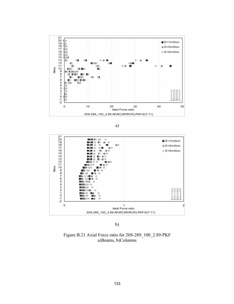
133
-2-10123456789
101112131415161718192021
0 10 20 30 40 50Axial Force ratio
Sto
ry
E=1million
E=3million
E=5million
20S-289_100_2.89-AF(RCSR/RCR)-PKF-E(7-11)
a)
-2-10123456789
101112131415161718192021
0 1 2Axial Force ratio
Stor
y
E=1million
E=3million
E=5million
20S-289_100_2.89-AF(RCSR/RCR)-PKF-E(7-11)
b)
Figure B.21 Axial Force ratio for 20S-289_100_2.89-PKF a)Beams, b)Columns

134
-2-10123456789
101112131415161718192021
0 10 20 30 40 50Axial Force ratio
Sto
ry
E=1million
E=3million
E=5million
20S-289_100_2.89-AF(RCSR/RCR)-ELC-E(7-11)
a)
-2-10123456789
101112131415161718192021
0 1 2Axial Force ratio
Stor
y
E=1million
E=3million
E=5million
20S-289_100_2.89-AF(RCSR/RCR)-ELC-E(7-11)
b)
Figure B.22 Axial Force ratio for 20S-289_100_2.89-ELC a)Beams, b)Columns
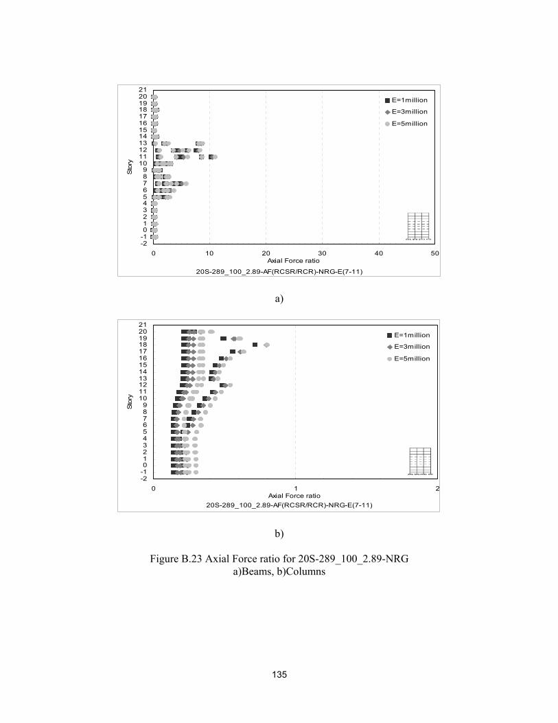
135
-2-10123456789
101112131415161718192021
0 10 20 30 40 50Axial Force ratio
Sto
ry
E=1million
E=3million
E=5million
20S-289_100_2.89-AF(RCSR/RCR)-NRG-E(7-11)
a)
-2-10123456789
101112131415161718192021
0 1 2Axial Force ratio
Stor
y
E=1million
E=3million
E=5million
20S-289_100_2.89-AF(RCSR/RCR)-NRG-E(7-11)
b)
Figure B.23 Axial Force ratio for 20S-289_100_2.89-NRG a)Beams, b)Columns

136
-2-10123456789
101112131415161718192021
0 10 20 30 40 50 60Axial Force ratio
Sto
ry
E=1million
E=3million
E=5million
20S-289_100_2.89-AF(RCSR/RCR)-KCL1-E(7-11)
a)
-2-10123456789
101112131415161718192021
0 1 2Axial Force ratio
Stor
y
E=1million
E=3million
E=5million
20S-289_100_2.89-AF(RCSR/RCR)-KCL1-E(7-11)
b)
Figure B.24 Axial Force ratio for 20S-289_100_2.89-KCL1 a)Beams, b)Columns

137
-2-10123456789
101112131415161718192021
0 30 60 90 120Axial Force ratio
Sto
ry
E=1million
E=3million
E=5million
20S-289_100_2.89-AF(RCSR/RCR)-KCL2-E(7-11)
a)
-2-10123456789
101112131415161718192021
0 1 2Axial Force ratio
Stor
y
E=1million
E=3million
E=5million
20S-289_100_2.89-AF(RCSR/RCR)-KCL2-E(7-11)
b)
Figure B.25 Axial Force ratio for 20S-289_100_2.89-KCL2 a)Beams, b)Columns

138
-2-10123456789
101112131415161718192021
0 1 2 3 4 5Axial Force ratio
Sto
ry
E=1million
E=3million
E=5million
20S-289_100_2.89-AF(RMSR/RMR)-PKF-E(7-11)
a)
-2-10123456789
101112131415161718192021
0 1 2 3 4 5Axial Force ratio
Stor
y
E=1million
E=3million
E=5million
20S-289_100_2.89-AF(RMSR/RMR)-PKF-E(7-11)
b)
Figure B.26 Axial Force ratio for 20S-289_100_2.89-PKF a)Beams, b)Columns

139
-2-10123456789
101112131415161718192021
0 1 2 3 4 5Axial Force ratio
Sto
ry
E=1million
E=3million
E=5million
20S-289_100_2.89-AF(RMSR/RMR)-ELC-E(7-11)
a)
-2-10123456789
101112131415161718192021
0 1 2 3 4 5Axial Force ratio
Stor
y
E=1million
E=3million
E=5million
20S-289_100_2.89-AF(RMSR/RMR)-ELC-E(7-11)
b)
Figure B.27 Axial Force ratio for 20S-289_100_2.89-ELC a)Beams, b)Columns

140
-2-10123456789
101112131415161718192021
0 1 2 3 4 5 6 7Axial Force ratio
Sto
ry
E=1million
E=3million
E=5million
20S-289_100_2.89-AF(RMSR/RMR)-NRG-E(7-11)
a)
-2-10123456789
101112131415161718192021
0 1 2 3 4 5Axial Force ratio
Stor
y
E=1million
E=3million
E=5million
20S-289_100_2.89-AF(RMSR/RMR)-NRG-E(7-11)
b)
Figure B.28 Axial Force ratio for 20S-289_100_2.89-NRG a)Beams, b)Columns

141
-2-10123456789
101112131415161718192021
0 5 10 15Axial Force ratio
Sto
ry
E=1million
E=3million
E=5million
20S-289_100_2.89-AF(RMSR/RMR)-KCL1-E(7-11)
a)
-2-10123456789
101112131415161718192021
0 1 2 3 4 5Axial Force ratio
Stor
y
E=1million
E=3million
E=5million
20S-289_100_2.89-AF(RMSR/RMR)-KCL1-E(7-11)
b)
Figure B.29 Axial Force ratio for 20S-289_100_2.89-KCL1 a)Beams, b)Columns

142
-2-10123456789
101112131415161718192021
0 5 10 15 20 25 30Axial Force ratio
Sto
ry
E=1million
E=3million
E=5million
20S-289_100_2.89-AF(RMSR/RMR)-KCL2-E(7-11)
a)
-2-10123456789
101112131415161718192021
0 1 2 3 4 5 6 7Axial Force ratio
Stor
y
E=1million
E=3million
E=5million
20S-289_100_2.89-AF(RMSR/RMR)-KCL2-E(7-11)
b)
Figure B.30 Axial Force ratio for 20S-289_100_2.89-KCL2 a)Beams, b)Columns

143
-10123456789
1011121314151617181920
0 40 80 120 160 200Axial Force ratio
Stor
y
Absolute AFmax ratio 20S-289_100_2.89-AF(RMR/RCSR)-PKF-E1m(7-11)
a)
-10123456789
101112131415161718192021
0 2 4 6 8 10Axial Force ratio
Stor
y
Absolute AFmax ratio 20S-289_100_2.89-AF(RMR/RCSR)-PKF-E1m(7-11)
b)
Figure B.31 Axial Force ratio for 20S-289_100_2.89-PKF a)Beams, b)Columns

144
-10123456789
1011121314151617181920
0 40 80 120 160 200Axial Force ratio
Stor
y
Absolute AFmax ratio 20S-289_100_2.89-AF(RMR/RCSR)-ELC-E1m(7-11)
a)
-10123456789
101112131415161718192021
0 1 2 3 4 5 6Axial Force ratio
Stor
y
Absolute AFmax ratio 20S-289_100_2.89-AF(RMR/RCSR)-ELC-E1m(7-11)
b)
Figure B.32 Axial Force ratio for 20S-289_100_2.89-ELC a)Beams, b)Columns

145
-10123456789
1011121314151617181920
0 20 40 60 80 100Axial Force ratio
Stor
y
Absolute AFmax ratio 20S-289_100_2.89-AF(RMR/RCSR)-NRG-E1m(7-11)
a)
-10123456789
101112131415161718192021
0 2 4 6 8 10Axial Force ratio
Stor
y
Absolute AFmax ratio 20S-289_100_2.89-AF(RMR/RCSR)-NRG-E1m(7-11)
b)
Figure B.33 Axial Force ratio for 20S-289_100_2.89-NRG a)Beams, b)Columns

146
-10123456789
1011121314151617181920
0 50 100 150 200 250Axial Force ratio
Stor
y
Absolute AFmax ratio 20S-289_100_2.89-AF(RMR/RCSR)-KCL1-E1m(7-11)
a)
-10123456789
101112131415161718192021
0 1 2 3 4 5Axial Force ratio
Stor
y
Absolute AFmax ratio 20S-289_100_2.89-AF(RMR/RCSR)-KCL1-E1m(7-11)
b)
Figure B.34 Axial Force ratio for 20S-289_100_2.89-KCL1 a)Beams, b)Columns

147
-10123456789
1011121314151617181920
0 30 60 90 120 150Axial Force ratio
Sto
ry
Absolute AFmax ratio 20S-289_100_2.89-AF(RMR/RCSR)-KCL2-E1m(7-11)
a)
-10123456789
101112131415161718192021
0 1 2 3 4 5Axial Force ratio
Sto
ry
Absolute AFmax ratio 20S-289_100_2.89-AF(RMR/RCSR)-KCL2-E1m(7-11)
b)
Figure B.35 Axial Force ratio for 20S-289_100_2.89-KCL2 a)Beams, b)Columns

148
-2-10123456789
101112131415161718192021
0 1 2 3 4 5 6Axial Force ratio
Sto
ry
E=1million
E=3million
E=5million
20S-289_300_0.963-AF(RMSR/RMR)-PKF-E(7-11)
a)
-2-10123456789
101112131415161718192021
0 1 2 3 4 5Axial Force ratio
Stor
y
E=1million
E=3million
E=5million
20S-289_300_0.963-AF(RMSR/RMR)-PKF-E(7-11)
b)
Figure B.36 Axial Force ratio for 20S-289_300_0.963-PKF a)Beams, b)Columns

149
-2-10123456789
101112131415161718192021
0 1 2 3 4 5 6Axial Force ratio
Sto
ry
E=1million
E=3million
E=5million
20S-289_300_0.963-AF(RMSR/RMR)-ELC-E(7-11)
a)
-2-10123456789
101112131415161718192021
0 1 2 3 4 5Axial Force ratio
Stor
y
E=1millionE=3millionE=5million
20S-289_300_0.963-AF(RMSR/RMR)-ELC-E(7-11)
b)
Figure B.37 Axial Force ratio for 20S-289_300_0.963-ELC a)Beams, b)Columns

150
-2-10123456789
101112131415161718192021
0 1 2 3 4 5 6 7 8 9 10Axial Force ratio
Sto
ry
E=1millionE=3million
E=5million
20S-289_300_0.963-AF(RMSR/RMR)-NRG-E(7-11)
a)
-2-10123456789
101112131415161718192021
0 1 2 3 4 5Axial Force ratio
Stor
y
E=1millionE=3million
E=5million
20S-289_300_0.963-AF(RMSR/RMR)-NRG-(7-11)
b)
Figure B.38 Axial Force ratio for 20S-289_300_0.963-NRG a)Beams, b)Columns

151
-2-10123456789
101112131415161718192021
0 1 2 3 4 5 6Axial Force ratio
Sto
ry
E=1million
E=3million
E=5million
20S-289_300_0.963-AF(RMSR/RMR)-KCL1-E(7-11)
a)
-2-10123456789
101112131415161718192021
0 1 2 3 4 5Axial Force ratio
Stor
y
E=1million
E=3million
E=5million
20S-289_300_0.963-AF(RMSR/RMR)-KCL1-E(7-11)
b)
Figure B.39 Axial Force ratio for 20S-289_300_0.963-KCL1 a)Beams, b)Columns

152
-2-10123456789
101112131415161718192021
0 1 2 3 4 5 6Axial Force ratio
Sto
ry
E=1million
E=3million
E=5million
20S-289_300_0.963-AF(RMSR/RMR)-KCL2-E(7-11)
a)
-2-10123456789
101112131415161718192021
0 1 2 3 4 5Axial Force ratio
Stor
y
E=1million
E=3million
E=5million
20S-289_300_0.963-AF(RMSR/RMR)-KCL2-E(7-11)
b)
Figure B.40 Axial Force ratio for 20S-289_300_0.963-KCL2 a)Beams, b)Columns

153
APPENDIX C
SHEAR FORCES IN THE FRAME ELEMENTS

154
0
1
2
3
0 0.2 0.4 0.6 0.8 1Shear Force ratio
Stor
y
Absolute SFmax ratio 3S-39_120_0.325-SF(RMR/RCR)-PKF
a)
0
1
2
3
4
0 0.2 0.4 0.6 0.8 1Shear Force ratio
Stor
y
Absolute SFmax ratio 3S-39_120_0.325-SF(RMR/RCR)-PKF
b)
Figure C.1 Shear Force ratio for 3S-39_120_0.325-PKF a)Beams, b)Columns

155
0
1
2
3
0 0.2 0.4 0.6 0.8 1Shear Force ratio
Stor
y
Absolute SFmax ratio 3S-39_120_0.325-SF(RMR/RCR)-ELC
a)
0
1
2
3
4
0 0.2 0.4 0.6 0.8 1Shear Force ratio
Stor
y
Absolute SFmax ratio 3S-39_120_0.325-SF(RMR/RCR)-ELC
b)
Figure C.2 Shear Force ratio for 3S-39_120_0.325-ELC a)Beams, b)Columns

156
0
1
2
3
0 0.2 0.4 0.6 0.8 1Shear Force ratio
Stor
y
Absolute SFmax ratio 3S-39_120_0.325-SF(RMR/RCR)-NRG
a)
0
1
2
3
4
0 0.2 0.4 0.6 0.8 1Shear Force ratio
Stor
y
Absolute SFmax ratio 3S-39_120_0.325-SF(RMR/RCR)-NRG
b)
Figure C.3 Shear Force ratio for 3S-39_120_0.325-NRG a)Beams, b)Columns

157
0
1
2
3
0 0.2 0.4 0.6 0.8 1Shear Force ratio
Stor
y
Absolute SFmax ratio 3S-39_120_0.325-SF(RMR/RCR)-KCL1
a)
0
1
2
3
4
0 0.2 0.4 0.6 0.8 1Shear Force ratio
Stor
y
Absolute SFmax ratio 3S-39_120_0.325-SF(RMR/RCR)-KCL1
b)
Figure C.4 Shear Force ratio for 3S-39_120_0.325-KCL1 a)Beams, b)Columns

158
0
1
2
3
0 0.2 0.4 0.6 0.8 1Shear Force ratio
Stor
y
Absolute SFmax ratio 3S-39_120_0.325-SF(RMR/RCR)-KCL2
a)
0
1
2
3
4
0 0.2 0.4 0.6 0.8 1Shear Force ratio
Stor
y
Absolute SFmax ratio 3S-39_120_0.325-SF(RMR/RCR)-KCL2
b)
Figure C.5 Shear Force ratio for 3S-39_120_0.325-KCL2 a)Beams, b)Columns

159
0
1
2
3
4
5
6
7
8
9
0 0.2 0.4 0.6 0.8 1Shear Force ratio
Stor
y
Absolute SFmax ratio 9S-134_150_0.893-SF(RMR/RCR)-PKF
a)
0
1
2
3
4
5
6
7
8
9
10
0 0.2 0.4 0.6 0.8 1Shear Force ratio
Stor
y
Absolute SFmax ratio 9S-134_150_0.893-SF(RMR/RCR)-PKF
b)
Figure C.6 Shear Force ratio for 9S-134_150_0.893-PKF a)Beams, b)Columns

160
0
1
2
3
4
5
6
7
8
9
0 0.2 0.4 0.6 0.8 1Shear Force ratio
Stor
y
Absolute SFmax ratio 9S-134_150_0.893-SF(RMR/RCR)-ELC
a)
0
1
2
3
4
5
6
7
8
9
10
0 0.3 0.6 0.9 1.2 1.5Shear Force ratio
Stor
y
Absolute SFmax ratio 9S-134_150_0.893-SF(RMR/RCR)-ELC
b)
Figure C.7 Shear Force ratio for 9S-134_150_0.893-ELC a)Beams, b)Columns

161
0
1
2
3
4
5
6
7
8
9
0 0.2 0.4 0.6 0.8 1Shear Force ratio
Stor
y
Absolute SFmax ratio 9S-134_150_0.893-SF(RMR/RCR)-NRG
a)
0
1
2
3
4
5
6
7
8
9
10
0 0.2 0.4 0.6 0.8 1Shear Force ratio
Stor
y
Absolute SFmax ratio 9S-134_150_0.893-SF(RMR/RCR)-NRG
b)
Figure C.8 Shear Force ratio for 9S-134_150_0.893-NRG a)Beams, b)Columns

162
0
1
2
3
4
5
6
7
8
9
0 0.2 0.4 0.6 0.8 1Shear Force ratio
Stor
y
Absolute SFmax ratio 9S-134_150_0.893-SF(RMR/RCR)-KCL1
a)
0
1
2
3
4
5
6
7
8
9
10
0 0.2 0.4 0.6 0.8 1Shear Force ratio
Stor
y
Absolute SFmax ratio 9S-134_150_0.893-SF(RMR/RCR)-KCL1
b)
Figure C.9 Shear Force ratio for 9S-134_150_0.893-KCL1 a)Beams, b)Columns

163
0
1
2
3
4
5
6
7
8
9
0 0.2 0.4 0.6 0.8 1Shear Force ratio
Stor
y
Absolute SFmax ratio 9S-134_150_0.893-SF(RMR/RCR)-KCL2
a)
0
1
2
3
4
5
6
7
8
9
10
0 0.2 0.4 0.6 0.8 1Shear Force ratio
Stor
y
Absolute SFmax ratio 9S-134_150_0.893-SF(RMR/RCR)-KCL2
b)
Figure C.10 Shear Force ratio for 9S-134_150_0.893-KCL2 a)Beams, b)Columns

164
0
1
2
3
4
5
6
7
8
9
10
11
12
0 0.5 1 1.5 2 2.5Shear Force ratio
Stor
y
Absolute SFmax ratio 12S-173_150_1.153-SF(RMR/RCR)-PKF
a)
0
1
2
3
4
5
6
7
8
9
10
11
12
13
0 0.4 0.8 1.2 1.6 2Shear Force ratio
Stor
y
Absolute SFmax ratio 12S-173_150_1.153-SF(RMR/RCR)-PKF
b)
Figure C.11 Shear Force ratio for 12S-173_150_1.153-PKF a)Beams, b)Columns

165
0
1
2
3
4
5
6
7
8
9
10
11
12
0 0.5 1 1.5 2Shear Force ratio
Stor
y
Absolute SFmax ratio 12S-173_150_1.153-SF(RMR/RCR)-ELC
a)
0
1
2
3
4
5
6
7
8
9
10
11
12
13
0 0.2 0.4 0.6 0.8 1Shear Force ratio
Stor
y
Absolute SFmax ratio 12S-173_150_1.153-SF(RMR/RCR)-ELC
b)
Figure C.12 Shear Force ratio for 12S-173_150_1.153-ELC a)Beams, b)Columns
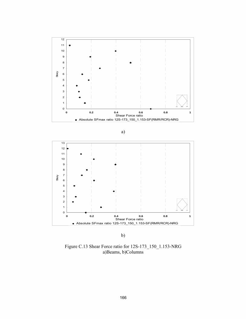
166
0
1
2
3
4
5
6
7
8
9
10
11
12
0 0.2 0.4 0.6 0.8 1Shear Force ratio
Stor
y
Absolute SFmax ratio 12S-173_150_1.153-SF(RMR/RCR)-NRG
a)
0
1
2
3
4
5
6
7
8
9
10
11
12
13
0 0.2 0.4 0.6 0.8 1Shear Force ratio
Stor
y
Absolute SFmax ratio 12S-173_150_1.153-SF(RMR/RCR)-NRG
b)
Figure C.13 Shear Force ratio for 12S-173_150_1.153-NRG a)Beams, b)Columns

167
0
1
2
3
4
5
6
7
8
9
10
11
12
0 0.5 1 1.5 2Shear Force ratio
Stor
y
Absolute SFmax ratio 12S-173_150_1.153-SF(RMR/RCR)-KCL1
a)
0
1
2
3
4
5
6
7
8
9
10
11
12
13
0 0.2 0.4 0.6 0.8 1Shear Force ratio
Stor
y
Absolute SFmax ratio 12S-173_150_1.153-SF(RMR/RCR)-KCL1
b)
Figure C.14 Shear Force ratio for 12S-173_150_1.153-KCL1 a)Beams, b)Columns

168
0
1
2
3
4
5
6
7
8
9
10
11
12
0 0.2 0.4 0.6 0.8 1Shear Force ratio
Sto
ry
Absolute SFmax ratio 12S-173_150_1.153-SF(RMR/RCR)-KCL2
a)
0
1
2
3
4
5
6
7
8
9
10
11
12
13
0 0.2 0.4 0.6 0.8 1Shear Force ratio
Sto
ry
Absolute SFmax ratio 12S-173_150_1.153-SF(RMR/RCR)-KCL2
b)
Figure C.15 Shear Force ratio for 12S-173_150_1.153-KCL2 a)Beams, b)Columns

169
-10123456789
1011121314151617181920
0 0.5 1 1.5 2 2.5Shear Force ratio
Stor
y
Absolute SFmax ratio 20S-289_100_2.89-SF(RMR/RCR)-PKF
a)
-10123456789
101112131415161718192021
0 0.5 1 1.5 2 2.5Shear Force ratio
Stor
y
Absolute SFmax ratio 20S-289_100_2.89-SF(RMR/RCR)-PKF
b)
Figure C.16 Shear Force ratio for 20S-289_100_2.89-PKF a)Beams, b)Columns

170
-10123456789
1011121314151617181920
0 0.5 1 1.5 2Shear Force ratio
Stor
y
Absolute SFmax ratio 20S-289_100_2.89-SF(RMR/RCR)-ELC
a)
-10123456789
101112131415161718192021
0 0.5 1 1.5Shear Force ratio
Stor
y
Absolute SFmax ratio 20S-289_100_2.89-SF(RMR/RCR)-ELC
b)
Figure C.17 Shear Force ratio for 20S-289_100_2.89-ELC a)Beams, b)Columns

171
-10123456789
1011121314151617181920
0 0.5 1 1.5Shear Force ratio
Stor
y
Absolute SFmax ratio 20S-289_100_2.89-SF(RMR/RCR)-NRG
a)
-10123456789
101112131415161718192021
0 0.5 1 1.5Shear Force ratio
Stor
y
Absolute SFmax ratio 20S-289_100_2.89-SF(RMR/RCR)-NRG
b)
Figure C.18 Shear Force ratio for 20S-289_100_2.89-NRG a)Beams, b)Columns

172
-10123456789
1011121314151617181920
0 1 2 3Shear Force ratio
Stor
y
Absolute SFmax ratio 20S-289_100_2.89-SF(RMR/RCR)-KCL1
a)
-10123456789
101112131415161718192021
0 0.5 1 1.5 2Shear Force ratio
Stor
y
Absolute SFmax ratio 20S-289_100_2.89-SF(RMR/RCR)-KCL1
b)
Figure C.19 Shear Force ratio for 20S-289_100_2.89-KCL1 a)Beams, b)Columns

173
-10123456789
1011121314151617181920
0 0.5 1 1.5 2Shear Force ratio
Sto
ry
Absolute SFmax ratio 20S-289_100_1.153-SF(RMR/RCR)-KCL2
a)
-10123456789
101112131415161718192021
0 0.5 1 1.5Shear Force ratio
Sto
ry
Absolute SFmax ratio 20S-289_100_2.89-SF(RMR/RCR)-KCL2
b)
Figure C.20 Shear Force ratio for 20S-289_100_2.89-KCL2 a)Beams, b)Columns

174
-2-10123456789
101112131415161718192021
0 0.5 1 1.5 2Shear Force ratio
Stor
y
E=1million
E=3million
E=5million
20S-289_100_2.89-SF(RCSR/RCR)-PKF-E(7-11)
a)
-2-10123456789
101112131415161718192021
0 1 2Shear Force ratio
Sto
ry
E=1million
E=3million
E=5million
20S-289_100_2.89-SF(RCSR/RCR)-PKF-E(7-11)
b)
Figure C.21 Shear Force ratio for 20S-289_100_2.89-PKF a)Beams, b)Columns

175
-2-10123456789
101112131415161718192021
0 0.5 1 1.5 2Shear Force ratio
Stor
y
E=1million
E=3million
E=5million
20S-289_100_2.89-SF(RCSR/RCR)-ELC-E(7-11)
a)
-2-10123456789
101112131415161718192021
0 1 2Shear Force ratio
Sto
ry
E=1million
E=3million
E=5million
20S-289_100_2.89-SF(RCSR/RCR)-ELC-E(7-11)
b)
Figure C.22 Shear Force ratio for 20S-289_100_2.89-ELC a)Beams, b)Columns

176
-2-10123456789
101112131415161718192021
0 0.5 1 1.5 2Shear Force ratio
Stor
y
E=1million
E=3million
E=5million
20S-289_100_2.89-SF(RCSR/RCR)-NRG-E(7-11)
a)
-2-10123456789
101112131415161718192021
0 1 2Shear Force ratio
Sto
ry
E=1million
E=3million
E=5million
20S-289_100_2.89-SF(RCSR/RCR)-NRG-E(7-11)
b)
Figure C.23 Shear Force ratio for 20S-289_100_2.89-NRG a)Beams, b)Columns

177
-2-10123456789
101112131415161718192021
0 0.5 1 1.5 2Shear Force ratio
Stor
y
E=1million
E=3million
E=5million
20S-289_100_2.89-SF(RCSR/RCR)-KCL1-E(7-11)
a)
-2-10123456789
101112131415161718192021
0 1 2Shear Force ratio
Sto
ry
E=1million
E=3million
E=5million
20S-289_100_2.89-SF(RCSR/RCR)-KCL1-E(7-11)
b)
Figure C.24 Shear Force ratio for 20S-289_100_2.89-KCL1 a)Beams, b)Columns

178
-2-10123456789
101112131415161718192021
0 1 2 3Shear Force ratio
Stor
y
E=1million
E=3million
E=5million
20S-289_100_2.89-SF(RCSR/RCR)-KCL2-E(7-11)
a)
-2-10123456789
101112131415161718192021
0 1 2Shear Force ratio
Sto
ry
E=1million
E=3million
E=5million
20S-289_100_2.89-SF(RCSR/RCR)-KCL2-E(7-11)
b)
Figure C.25 Shear Force ratio for 20S-289_100_2.89-KCL2 a)Beams, b)Columns

179
-2-10123456789
101112131415161718192021
0 1 2 3 4 5Shear Force ratio
Stor
y
E=1million
E=3million
E=5million
20S-289_100_2.89-SF(RMSR/RMR)-PKF-E(7-11)
a)
-2-10123456789
101112131415161718192021
0 1 2 3 4 5Shear Force ratio
Sto
ry
E=1million
E=3million
E=5million
20S-289_100_2.89-SF(RMSR/RMR)-PKF-E(7-11)
b)
Figure C.26 Shear Force ratio for 20S-289_100_2.89-PKF a)Beams, b)Columns

180
-2-10123456789
101112131415161718192021
0 1 2 3 4 5Shear Force ratio
Stor
y
E=1million
E=3million
E=5million
20S-289_100_2.89-SF(RMSR/RMR)-ELC-E(7-11)
a)
-2-10123456789
101112131415161718192021
0 1 2 3 4 5Shear Force ratio
Sto
ry
E=1million
E=3million
E=5million
20S-289_100_2.89-SF(RMSR/RMR)-ELC-E(7-11)
b)
Figure C.27 Shear Force ratio for 20S-289_100_2.89-ELC a)Beams, b)Columns

181
-2-10123456789
101112131415161718192021
0 1 2 3 4 5Shear Force ratio
Stor
y
E=1million
E=3million
E=5million
20S-289_100_2.89-SF(RMSR/RMR)-NRG-E(7-11)
a)
-2-10123456789
101112131415161718192021
0 1 2 3 4 5Shear Force ratio
Sto
ry
E=1million
E=3million
E=5million
20S-289_100_2.89-SF(RMSR/RMR)-NRG-E(7-11)
b)
Figure C.28 Shear Force ratio for 20S-289_100_2.89-NRG a)Beams, b)Columns

182
-2-10123456789
101112131415161718192021
0 1 2 3 4 5Shear Force ratio
Stor
y
E=1million
E=3million
E=5million
20S-289_100_2.89-SF(RMSR/RMR)-KCL1-E(7-11)
a)
-2-10123456789
101112131415161718192021
0 1 2 3 4 5Shear Force ratio
Sto
ry
E=1million
E=3million
E=5million
20S-289_100_2.89-SF(RMSR/RMR)-KCL1-E(7-11)
b)
Figure C.29 Shear Force ratio for 20S-289_100_2.89-KCL1 a)Beams, b)Columns

183
-2-10123456789
101112131415161718192021
0 1 2 3 4 5Shear Force ratio
Stor
y
E=1million
E=3million
E=5million
20S-289_100_2.89-SF(RMSR/RMR)-KCL2-E(7-11)
a)
-2-10123456789
101112131415161718192021
0 1 2 3 4 5Shear Force ratio
Sto
ry
E=1million
E=3million
E=5million
20S-289_100_2.89-SF(RMSR/RMR)-KCL2-E(7-11)
b)
Figure C.30 Shear Force ratio for 20S-289_100_2.89-KCL2 a)Beams, b)Columns

184
-10123456789
1011121314151617181920
0 1 2 3 4 5Shear Force ratio
Stor
y
Absolute SFmax ratio 20S-289_100_2.89-SF(RMR/RCSR)-PKF-E1m(7-11)
a)
-10123456789
101112131415161718192021
0 1 2 3 4 5Shear Force ratio
Stor
y
Absolute SFmax ratio 20S-289_100_2.89-SF(RMR/RCSR)-PKF-E1m(7-11)
b)
Figure C.31 Shear Force ratio for 20S-289_100_2.89-PKF a)Beams, b)Columns

185
-10123456789
1011121314151617181920
0 1 2 3 4 5Shear Force ratio
Stor
y
Absolute SFmax ratio 20S-289_100_2.89-SF(RMR/RCSR)-ELC-E1m(7-11)
a)
-10123456789
101112131415161718192021
0 1 2 3Shear Force ratio
Stor
y
Absolute SFmax ratio 20S-289_100_2.89-SF(RMR/RCSR)-ELC-E1m(7-11)
b)
Figure C.32 Shear Force ratio for 20S-289_100_2.89-ELC a)Beams, b)Columns

186
-10123456789
1011121314151617181920
0 1 2 3 4 5Shear Force ratio
Stor
y
Absolute SFmax ratio 20S-289_100_2.89-SF(RMR/RCSR)-NRG-E1m(7-11)
a)
-10123456789
101112131415161718192021
0 1 2 3Shear Force ratio
Stor
y
Absolute SFmax ratio 20S-289_100_2.89-SF(RMR/RCSR)-NRG-E1m(7-11)
b)
Figure C.33 Shear Force ratio for 20S-289_100_2.89-NRG a)Beams, b)Columns

187
-10123456789
1011121314151617181920
0 1 2 3 4 5Shear Force ratio
Stor
y
Absolute SFmax ratio 20S-289_100_2.89-SF(RMR/RCSR)-KCL1-E1m(7-11)
a)
-10123456789
101112131415161718192021
0 1 2 3Shear Force ratio
Stor
y
Absolute SFmax ratio 20S-289_100_2.89-SF(RMR/RCSR)-KCL1-E1m(7-11)
b)
Figure C.34 Shear Force ratio for 20S-289_100_2.89-KCL1 a)Beams, b)Columns

188
-10123456789
1011121314151617181920
0 1 2 3Shear Force ratio
Sto
ry
Absolute SFmax ratio 20S-289_100_1.153-SF(RMR/RCSR)-KCL2-E1m(7-11)
a)
-10123456789
101112131415161718192021
0 1 2Shear Force ratio
Sto
ry
Absolute SFmax ratio 20S-289_100_2.89-SF(RMR/RCSR)-KCL2-E1m(7-11)
b)
Figure C.35 Shear Force ratio for 20S-289_100_2.89-KCL2 a)Beams, b)Columns

189
-2-10123456789
101112131415161718192021
0 1 2 3 4 5Shear Force ratio
Stor
y
E=1million
E=3million
E=5million
20S-289_300_0.963-SF(RMSR/RMR)-PKF-E(7-11)
a)
-2-10123456789
101112131415161718192021
0 1 2 3 4 5Shear Force ratio
Sto
ry
E=1million
E=3million
E=5million
20S-289_300_0.963-SF(RMSR/RMR)-PKF-E(7-11)
b)
Figure C.36 Shear Force ratio for 20S-289_300_0.963-PKF a)Beams, b)Columns

190
-2-10123456789
101112131415161718192021
0 1 2 3 4 5Shear Force ratio
Stor
y
E=1millionE=3millionE=5million
20S-289_300_0.963-SF(RMSR/RMR)-ELC-E(7-11)
a)
-2-10123456789
101112131415161718192021
0 1 2 3 4 5Shear Force ratio
Sto
ry
E=1million
E=3million
E=5million
20S-289_300_0.963-SF(RMSR/RMR)-ELC-E(7-11)
b)
Figure C.37 Shear Force ratio for 20S-289_300_0.963-ELC a)Beams, b)Columns

191
-2-10123456789
101112131415161718192021
0 1 2 3 4 5 6 7 8Shear Force ratio
Stor
y
E=1millionE=3million
E=5million
20S-289_300_0.963-SF(RMSR/RMR)-NRG-E(7-11)
a)
-2-10123456789
101112131415161718192021
0 1 2 3 4 5 6 7 8Shear Force ratio
Sto
ry
E=1million
E=3million
E=5million
20S-289_300_0.963-SF(RMSR/RMR)-NRG-(7-11)
b)
Figure C.38 Shear Force ratio for20S-289_300_0.963-NRG a)Beams, b)Columns

192
-2-10123456789
101112131415161718192021
0 1 2 3 4 5 6 7Shear Force ratio
Stor
y
E=1million
E=3million
E=5million
20S-289_300_0.963-SF(RMSR/RMR)-KCL1-E(7-11)
a)
-2-10123456789
101112131415161718192021
0 1 2 3 4 5 6 7Shear Force ratio
Sto
ry
E=1million
E=3million
E=5million
20S-289_300_0.963-SF(RMSR/RMR)-KCL1-E(7-11)
b)
Figure C.39 Shear Force ratio for20S-289_300_0.963-KCL1 a)Beams, b)Columns

193
-2-10123456789
101112131415161718192021
0 1 2 3 4 5 6Shear Force ratio
Stor
y
E=1million
E=3million
E=5million
20S-289_300_0.963-SF(RMSR/RMR)-KCL2-E(7-11)
a)
-2-10123456789
101112131415161718192021
0 1 2 3 4 5Shear Force ratio
Sto
ry
E=1million
E=3million
E=5million
20S-289_300_0.963-SF(RMSR/RMR)-KCL2-E(7-11)
b)
Figure C.40 Shear Force ratio for 20S-289_300_0.963-KCL2 a)Beams, b)Columns

194
APPENDIX D
BENDING MOMENTS IN THE FRAME ELEMENTS

195
0
1
2
3
0 0.2 0.4 0.6 0.8 1Bending Moment ratio
Stor
y
Absolute BMmax ratio 3S-39_120_0.325-BM(RMR/RCR)-PKF
a)
0
1
2
3
4
0 0.2 0.4 0.6 0.8 1Bending Moment ratio
Stor
y
Absolute BMmax ratio 3S-39_120_0.325-BM(RMR/RCR)-PKF
b)
Figure D.1 Bending Moment ratio for 3S-39_120_0.325-PKF a)Beams, b)Columns

196
0
1
2
3
0 0.2 0.4 0.6 0.8 1Bending Moment ratio
Stor
y
Absolute BMmax ratio 3S-39_120_0.325-BM(RMR/RCR)-ELC
a)
0
1
2
3
4
0 0.2 0.4 0.6 0.8 1Bending Moment ratio
Stor
y
Absolute BMmax ratio 3S-39_120_0.325-BM(RMR/RCR)-ELC
b)
Figure D.2 Bending Moment ratio for 3S-39_120_0.325-ELC a)Beams, b)Columns

197
0
1
2
3
0 0.2 0.4 0.6 0.8 1Bending Moment ratio
Stor
y
Absolute BMmax ratio 3S-39_120_0.325-BM(RMR/RCR)-NRG
a)
0
1
2
3
4
0 0.2 0.4 0.6 0.8 1Bending Moment ratio
Stor
y
Absolute BMmax ratio 3S-39_120_0.325-BM(RMR/RCR)-NRG
b)
Figure D.3 Bending Moment ratio for 3S-39_120_0.325-NRG a)Beams, b)Columns

198
0
1
2
3
0 0.2 0.4 0.6 0.8 1Bending Moment ratio
Stor
y
Absolute BMmax ratio 3S-39_120_0.325-BM(RMR/RCR)-KCL1
a)
0
1
2
3
4
0 0.2 0.4 0.6 0.8 1Bending Moment ratio
Stor
y
Absolute BMmax ratio 3S-39_120_0.325-BM(RMR/RCR)-KCL1
b)
Figure D.4 Bending Moment ratio for 3S-39_120_0.325-KCL1 a)Beams, b)Columns

199
0
1
2
3
0 0.2 0.4 0.6 0.8 1Bending Moment ratio
Stor
y
Absolute BMmax ratio 3S-39_120_0.325-BM(RMR/RCR)-KCL2
a)
0
1
2
3
4
0 0.2 0.4 0.6 0.8 1Bending Moment ratio
Stor
y
Absolute BMmax ratio 3S-39_120_0.325-BM(RMR/RCR)-KCL2
b)
Figure D.5 Bending Moment ratio for 3S-39_120_0.325-KCL2 a)Beams, b)Columns

200
0
1
2
3
4
5
6
7
8
9
0 0.2 0.4 0.6 0.8 1Bending Moment ratio
Stor
y
Absolute BMmax ratio 9S-134_150_0.893-BM(RMR/RCR)-PKF
a)
0
1
2
3
4
5
6
7
8
9
10
0 0.2 0.4 0.6 0.8 1Bending Moment ratio
Stor
y
Absolute BMmax ratio 9S-134_150_0.893-BM(RMR/RCR)-PKF
b)
Figure D.6 Bending Moment ratio for 9S-134_150_0.893-PKF a)Beams, b)Columns

201
0
1
2
3
4
5
6
7
8
9
0 0.2 0.4 0.6 0.8 1Bending Moment ratio
Stor
y
Absolute BMmax ratio 9S-134_150_0.893-BM(RMR/RCR)-ELC
a)
0
1
2
3
4
5
6
7
8
9
10
0 0.3 0.6 0.9 1.2 1.5Bending Moment ratio
Stor
y
Absolute BMmax ratio 9S-134_150_0.893-BM(RMR/RCR)-ELC
b)
Figure D.7 Bending Moment ratio for 9S-134_150_0.893-ELC a)Beams, b)Columns

202
0
1
2
3
4
5
6
7
8
9
0 0.2 0.4 0.6 0.8 1Bending Moment ratio
Stor
y
Absolute BMmax ratio 9S-134_150_0.893-BM(RMR/RCR)-NRG
a)
0
1
2
3
4
5
6
7
8
9
10
0 0.2 0.4 0.6 0.8 1Bending Moment ratio
Stor
y
Absolute BMmax ratio 9S-134_150_0.893-BM(RMR/RCR)-NRG
b)
Figure D.8 Bending Moment ratio for 9S-134_150_0.893-NRG a)Beams, b)Columns

203
0
1
2
3
4
5
6
7
8
9
0 0.2 0.4 0.6 0.8 1Bending Moment ratio
Stor
y
Absolute BMmax ratio 9S-134_150_0.893-BM(RMR/RCR)-KCL1
a)
0
1
2
3
4
5
6
7
8
9
10
0 0.2 0.4 0.6 0.8 1Bending Moment ratio
Stor
y
Absolute BMmax ratio 9S-134_150_0.893-BM(RMR/RCR)-KCL1
b)
Figure D.9 Bending Moment ratio for 9S-134_150_0.893-KCL1 a)Beams, b)Columns

204
0
1
2
3
4
5
6
7
8
9
0 0.2 0.4 0.6 0.8 1Bending Moment ratio
Stor
y
Absolute BMmax ratio 9S-134_150_0.893-BM(RMR/RCR)-KCL2
a)
0
1
2
3
4
5
6
7
8
9
10
0 0.2 0.4 0.6 0.8 1Bending Moment ratio
Stor
y
Absolute BMmax ratio 9S-134_150_0.893-BM(RMR/RCR)-KCL2
b)
Figure D.10 Bending Moment ratio for 9S-134_150_0.893-KCL2 a)Beams, b)Columns

205
0
1
2
3
4
5
6
7
8
9
10
11
12
0 1 2Bending Moment ratio
Stor
y
Absolute BMmax ratio 12S-173_150_1.153-BM(RMR/RCR)-PKF
a)
0
1
2
3
4
5
6
7
8
9
10
11
12
13
0 1 2Bending Moment ratio
Stor
y
Absolute BMmax ratio 12S-173_150_1.153-BM(RMR/RCR)-PKF
b)
Figure D.11 Bending Moment ratio for 12S-173_150_1.153-PKF a)Beams, b)Columns

206
0
1
2
3
4
5
6
7
8
9
10
11
12
0 0.2 0.4 0.6 0.8 1Bending Moment ratio
Stor
y
Absolute BMmax ratio 12S-173_150_1.153-BM(RMR/RCR)-ELC
a)
0
1
2
3
4
5
6
7
8
9
10
11
12
13
0 0.2 0.4 0.6 0.8 1Bending Moment ratio
Stor
y
Absolute BMmax ratio 12S-173_150_1.153-BM(RMR/RCR)-ELC
b)
Figure D.12 Bending Moment ratio for 12S-173_150_1.153-ELC a)Beams, b)Columns
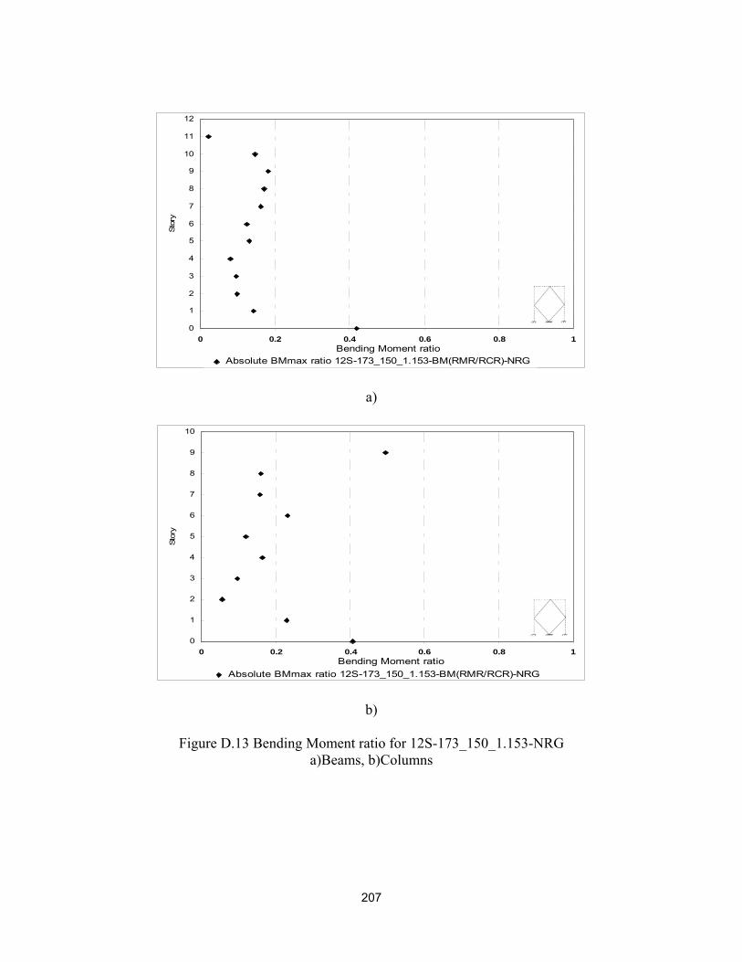
207
0
1
2
3
4
5
6
7
8
9
10
11
12
0 0.2 0.4 0.6 0.8 1Bending Moment ratio
Stor
y
Absolute BMmax ratio 12S-173_150_1.153-BM(RMR/RCR)-NRG
a)
0
1
2
3
4
5
6
7
8
9
10
0 0.2 0.4 0.6 0.8 1Bending Moment ratio
Stor
y
Absolute BMmax ratio 12S-173_150_1.153-BM(RMR/RCR)-NRG
b)
Figure D.13 Bending Moment ratio for 12S-173_150_1.153-NRG a)Beams, b)Columns
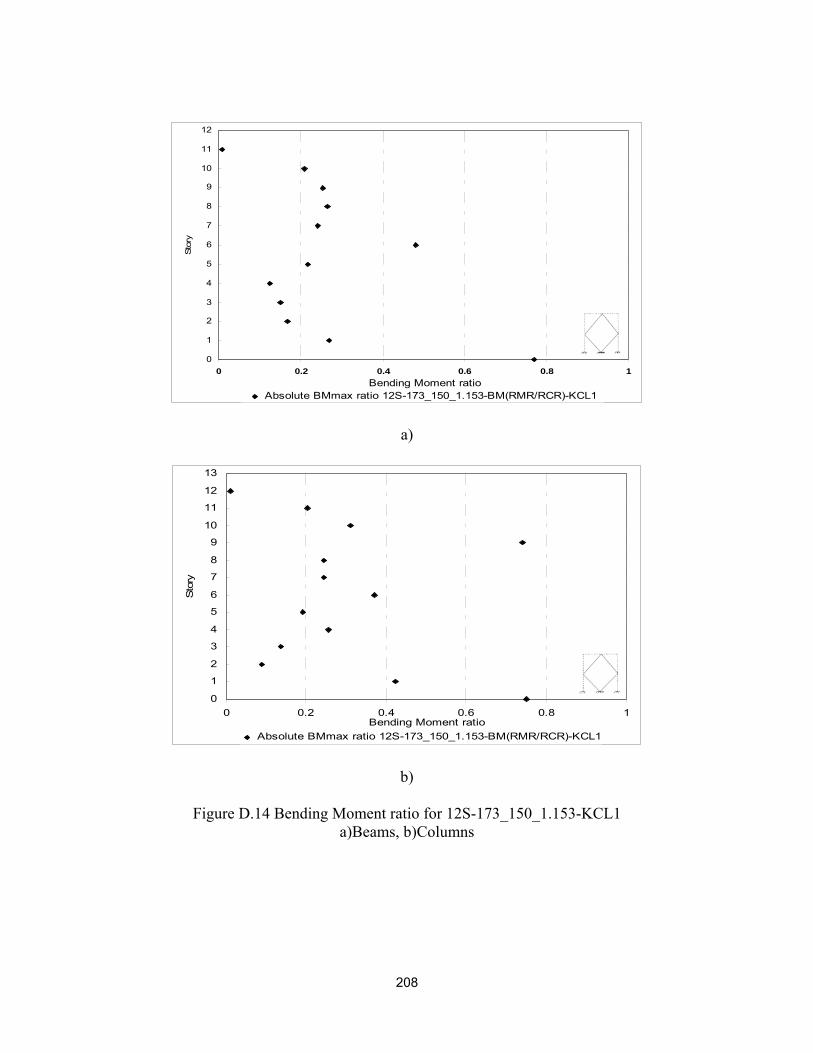
208
0
1
2
3
4
5
6
7
8
9
10
11
12
0 0.2 0.4 0.6 0.8 1Bending Moment ratio
Stor
y
Absolute BMmax ratio 12S-173_150_1.153-BM(RMR/RCR)-KCL1
a)
0
1
2
3
4
5
6
7
8
9
10
11
12
13
0 0.2 0.4 0.6 0.8 1Bending Moment ratio
Sto
ry
Absolute BMmax ratio 12S-173_150_1.153-BM(RMR/RCR)-KCL1
b)
Figure D.14 Bending Moment ratio for 12S-173_150_1.153-KCL1 a)Beams, b)Columns

209
0
1
2
3
4
5
6
7
8
9
10
11
12
0 0.2 0.4 0.6 0.8 1Bending Moment ratio
Sto
ry
Absolute BMmax ratio 12S-173_150_1.153-BM(RMR/RCR)-KCL2
a)
0
1
2
3
4
5
6
7
8
9
10
11
12
13
0 0.2 0.4 0.6 0.8 1Bending Moment ratio
Sto
ry
Absolute BMmax ratio 12S-173_150_1.153-BM(RMR/RCR)-KCL2
b)
Figure D.15 Bending Moment ratio for 12S-173_150_1.153-KCL2 a)Beams, b)Columns

210
-10123456789
1011121314151617181920
0 1 2 3Bending Moment ratio
Stor
y
Absolute BMmax ratio 20S-289_100_2.89-BM(RMR/RCR)-PKF
a)
-10123456789
101112131415161718192021
0 1 2 3 4 5 6Bending Moment ratio
Stor
y
Absolute BMmax ratio 20S-289_100_2.89-BM(RMR/RCR)-PKF
b)
Figure D.16 Bending Moment ratio for 20S-289_100_2.89-PKF a)Beams, b)Columns

211
0123456789
1011121314151617181920
0 0.5 1 1.5Bending Moment ratio
Stor
y
Absolute BMmax ratio 20S-289_100_2.89-BM(RMR/RCR)-ELC
a)
-10123456789
101112131415161718192021
0 1 2 3Bending Moment ratio
Stor
y
Absolute BMmax ratio 20S-289_100_2.89-BM(RMR/RCR)-ELC
b)
Figure D.17 Bending Moment ratio for 20S-289_100_2.89-ELC a)Beams, b)Columns

212
-10123456789
1011121314151617181920
0 0.5 1 1.5Bending Moment ratio
Stor
y
Absolute BMmax ratio 20S-289_100_2.89-BM(RMR/RCR)-NRG
a)
-10123456789
101112131415161718192021
0 1 2 3Bending Moment ratio
Stor
y
Absolute BMmax ratio 20S-289_100_2.89-BM(RMR/RCR)-NRG
b)
Figure D.18 Bending Moment ratio for 20S-289_100_2.89-NRG a)Beams, b)Columns

213
-10123456789
1011121314151617181920
0 0.5 1 1.5 2 2.5Bending Moment ratio
Stor
y
Absolute BMmax ratio 20S-289_100_2.89-BM(RMR/RCR)-KCL1
a)
-10123456789
101112131415161718192021
0 1 2 3 4 5 6Bending Moment ratio
Sto
ry
Absolute BMmax ratio 20S-289_100_2.89-BM(RMR/RCR)-KCL1
b)
Figure D.19 Bending Moment ratio for 20S-289_100_2.89-KCL1 a)Beams, b)Columns
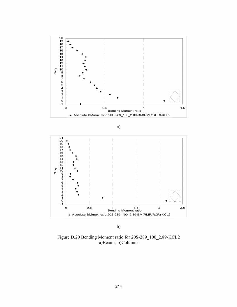
214
-10123456789
1011121314151617181920
0 0.5 1 1.5Bending Moment ratio
Sto
ry
Absolute BMmax ratio 20S-289_100_2.89-BM(RMR/RCR)-KCL2
a)
-10123456789
101112131415161718192021
0 0.5 1 1.5 2 2.5Bending Moment ratio
Sto
ry
Absolute BMmax ratio 20S-289_100_2.89-BM(RMR/RCR)-KCL2
b)
Figure D.20 Bending Moment ratio for 20S-289_100_2.89-KCL2 a)Beams, b)Columns

215
-2-10123456789
101112131415161718192021
0 0.5 1 1.5 2Bending Moment ratio
Sto
ry
E=1million
E=3million
E=5million
20S-289_100_2.89-BM(RCSR/RCR)-PKF-E(7-11)
a)
-2-10123456789
101112131415161718192021
0 1 2 3Bending Moment ratio
Stor
y
E=1million
E=3million
E=5million
20S-289_100_2.89-BM(RCSR/RCR)-PKF-E(7-11)
b)
Figure D.21 Bending Moment ratio for 20S-289_100_2.89-PKF a)Beams, b)Columns

216
-2-10123456789
101112131415161718192021
0 0.5 1 1.5 2Bending Moment ratio
Sto
ry
E=1million
E=3million
E=5million
20S-289_100_2.89-BM(RCSR/RCR)-ELC-E(7-11)
a)
-2-10123456789
101112131415161718192021
0 1 2 3Bending Moment ratio
Stor
y
E=1million
E=3million
E=5million
20S-289_100_2.89-BM(RCSR/RCR)-ELC-E(7-11)
b)
Figure D.22 Bending Moment ratio for 20S-289_100_2.89-ELC a)Beams, b)Columns

217
-2-10123456789
101112131415161718192021
0 0.5 1 1.5 2Bending Moment ratio
Sto
ry
E=1million
E=3million
E=5million
20S-289_100_2.89-BM(RCSR/RCR)-NRG-E(7-11)
a)
-2-10123456789
101112131415161718192021
0 1 2 3Bending Moment ratio
Stor
y
E=1million
E=3million
E=5million
20S-289_100_2.89-BM(RCSR/RCR)-NRG-E(7-11)
b)
Figure D.23 Bending Moment ratio for 20S-289_100_2.89-NRG a)Beams, b)Columns

218
-2-10123456789
101112131415161718192021
0 0.5 1 1.5 2Bending Moment ratio
Sto
ry
E=1million
E=3million
E=5million
20S-289_100_2.89-BM(RCSR/RCR)-KCL1-E(7-11)
a)
-2-10123456789
101112131415161718192021
0 1 2 3Bending Moment ratio
Stor
y
E=1million
E=3million
E=5million
20S-289_100_2.89-BM(RCSR/RCR)-KCL1-E(7-11)
b)
Figure D.24 Bending Moment ratio for 20S-289_100_2.89-KCL1 a)Beams, b)Columns

219
-2-10123456789
101112131415161718192021
0 1 2 3Bending Moment ratio
Sto
ry
E=1million
E=3million
E=5million
20S-289_100_2.89-BM(RCSR/RCR)-KCL2-E(7-11)
a)
-2-10123456789
101112131415161718192021
0 1 2 3Bending Moment ratio
Stor
y
E=1million
E=3million
E=5million
20S-289_100_2.89-BM(RCSR/RCR)-KCL2-E(7-11)
b)
Figure D.25 Bending Moment ratio for 20S-289_100_2.89-KCL2 a)Beams, b)Columns
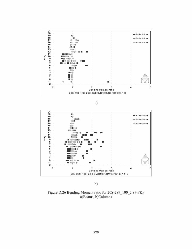
220
-2-10123456789
101112131415161718192021
0 1 2 3 4 5Bending Moment ratio
Sto
ry
E=1million
E=3million
E=5million
20S-289_100_2.89-BM(RMSR/RMR)-PKF-E(7-11)
a)
-2-10123456789
101112131415161718192021
0 1 2 3 4 5Bending Moment ratio
Stor
y
E=1million
E=3million
E=5million
20S-289_100_2.89-BM(RMSR/RMR)-PKF-E(7-11)
b)
Figure D.26 Bending Moment ratio for 20S-289_100_2.89-PKF a)Beams, b)Columns
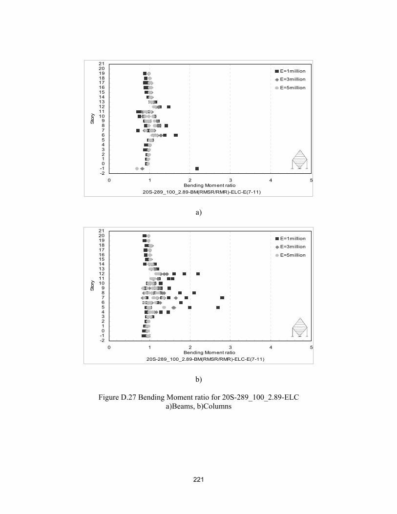
221
-2-10123456789
101112131415161718192021
0 1 2 3 4 5Bending Moment ratio
Sto
ry
E=1million
E=3million
E=5million
20S-289_100_2.89-BM(RMSR/RMR)-ELC-E(7-11)
a)
-2-10123456789
101112131415161718192021
0 1 2 3 4 5Bending Moment ratio
Stor
y
E=1million
E=3million
E=5million
20S-289_100_2.89-BM(RMSR/RMR)-ELC-E(7-11)
b)
Figure D.27 Bending Moment ratio for 20S-289_100_2.89-ELC a)Beams, b)Columns

222
-2-10123456789
101112131415161718192021
0 1 2 3 4 5Bending Moment ratio
Sto
ry
E=1million
E=3million
E=5million
20S-289_100_2.89-BM(RMSR/RMR)-NRG-E(7-11)
a)
-2-10123456789
101112131415161718192021
0 1 2 3 4 5Bending Moment ratio
Stor
y
E=1million
E=3million
E=5million
20S-289_100_2.89-BM(RMSR/RMR)-NRG-E(7-11)
b)
Figure D.28 Bending Moment ratio for 20S-289_100_2.89-NRG a)Beams, b)Columns

223
-2-10123456789
101112131415161718192021
0 1 2 3 4 5Bending Moment ratio
Sto
ry
E=1million
E=3million
E=5million
20S-289_100_2.89-BM(RMSR/RMR)-KCL1-E(7-11)
a)
-2-10123456789
101112131415161718192021
0 1 2 3 4 5Bending Moment ratio
Stor
y
E=1million
E=3million
E=5million
20S-289_100_2.89-BM(RMSR/RMR)-KCL1-E(7-11)
b)
Figure D.29 Bending Moment ratio for 20S-289_100_2.89-KCL1 a)Beams, b)Columns

224
-2-10123456789
101112131415161718192021
0 1 2 3 4 5Bending Moment ratio
Sto
ry
E=1million
E=3million
E=5million
20S-289_100_2.89-BM(RMSR/RMR)-KCL2-E(7-11)
a)
-2-10123456789
101112131415161718192021
0 1 2 3 4 5Bending Moment ratio
Stor
y
E=1million
E=3million
E=5million
20S-289_100_2.89-BM(RMSR/RMR)-KCL2-E(7-11)
b)
Figure D.30 Bending Moment ratio for 20S-289_100_2.89-KCL2 a)Beams, b)Columns

225
-10123456789
1011121314151617181920
0 1 2 3 4 5Bending Moment ratio
Stor
y
Absolute BMmax ratio 20S-289_100_2.89-BM(RMR/RCSR)-PKF-E1m(7-11)
a)
-10123456789
101112131415161718192021
0 1 2 3 4 5 6 7Bending Moment ratio
Stor
y
Absolute BMmax ratio 20S-289_100_2.89-BM(RMR/RCSR)-PKF-E1m(7-11)
b)
Figure D.31 Bending Moment ratio for 20S-289_100_2.89-PKF a)Beams, b)Columns

226
0123456789
1011121314151617181920
0 1 2 3Bending Moment ratio
Stor
y
Absolute BMmax ratio 20S-289_100_2.89-BM(RMR/RCSR)-ELC-E1m(7-11)
a)
-10123456789
101112131415161718192021
0 1 2 3Bending Moment ratio
Stor
y
Absolute BMmax ratio 20S-289_100_2.89-BM(RMR/RCSR)-ELC-E1m(7-11)
b)
Figure D.32 Bending Moment ratio for 20S-289_100_2.89-ELC a)Beams, b)Columns

227
-10123456789
1011121314151617181920
0 1 2 3 4 5Bending Moment ratio
Stor
y
Absolute BMmax ratio 20S-289_100_2.89-BM(RMR/RCSR)-NRG-E1m(7-11)
a)
-10123456789
101112131415161718192021
0 1 2 3Bending Moment ratio
Stor
y
Absolute BMmax ratio 20S-289_100_2.89-BM(RMR/RCSR)-NRG-E1m(7-11)
b)
Figure D.33 Bending Moment ratio for 20S-289_100_2.89-NRG a)Beams, b)Columns

228
-10123456789
1011121314151617181920
0 1 2 3Bending Moment ratio
Stor
y
Absolute BMmax ratio 20S-289_100_2.89-BM(RMR/RCSR)-KCL1-E1m(7-11)
a)
-10123456789
101112131415161718192021
0 1 2 3Bending Moment ratio
Sto
ry
Absolute BMmax ratio 20S-289_100_2.89-BM(RMR/RCSR)-KCL1-E1m(7-11)
b)
Figure D.34 Bending Moment ratio for 20S-289_100_2.89-KCL1 a)Beams, b)Columns

229
-10123456789
1011121314151617181920
0 1 2Bending Moment ratio
Sto
ry
Absolute BMmax ratio 20S-289_100_2.89-BM(RMR/RCSR)-KCL2-E1m(7-11)
a)
-10123456789
101112131415161718192021
0 1 2Bending Moment ratio
Sto
ry
Absolute BMmax ratio 20S-289_100_2.89-BM(RMR/RCSR)-KCL2-E1m(7-11)
b)
Figure D.35 Bending Moment ratio for 20S-289_100_2.89-KCL2 a)Beams, b)Columns

230
-2-10123456789
101112131415161718192021
0 1 2 3 4 5Bending Moment ratio
Sto
ry
E=1million
E=3million
E=5million
20S-289_300_0.963-BM(RMSR/RMR)-PKF-E(7-11)
a)
-2-10123456789
101112131415161718192021
0 1 2 3 4 5Bending Moment ratio
Stor
y
E=1million
E=3million
E=5million
20S-289_300_0.963-BM(RMSR/RMR)-PKF-E(7-11)
b)
Figure D.36 Bending Moment ratio for 20S-289_300_0.963-PKF a)Beams, b)Columns

231
-2-10123456789
101112131415161718192021
0 1 2 3 4 5Bending Moment ratio
Sto
ry
E=1million
E=3million
E=5million
20S-289_300_0.963-BM(RMSR/RMR)-ELC-E(7-11)
a)
-2-10123456789
101112131415161718192021
0 1 2 3 4 5Bending Moment ratio
Stor
y
E=1millionE=3million
E=5million
20S-289_300_0.963-BM(RMSR/RMR)-ELC-E(7-11)
b)
Figure D.37 Bending Moment ratio for 20S-289_300_0.963-ELC a)Beams, b)Columns

232
-2-10123456789
101112131415161718192021
0 1 2 3 4 5 6 7 8Bending Moment ratio
Sto
ry
E=1million
E=3million
E=5million
20S-289_300_0.963-BM(RMSR/RMR)-NRG-E(7-11)
a)
-2-10123456789
101112131415161718192021
0 1 2 3 4 5Bending Moment ratio
Stor
y
E=1millionE=3million
E=5million
20S-289_300_0.963-BM(RMSR/RMR)-NRG-E(7-11)
b)
Figure D.38 Bending Moment ratio for 20S-289_300_0.963-NRG a)Beams, b)Columns
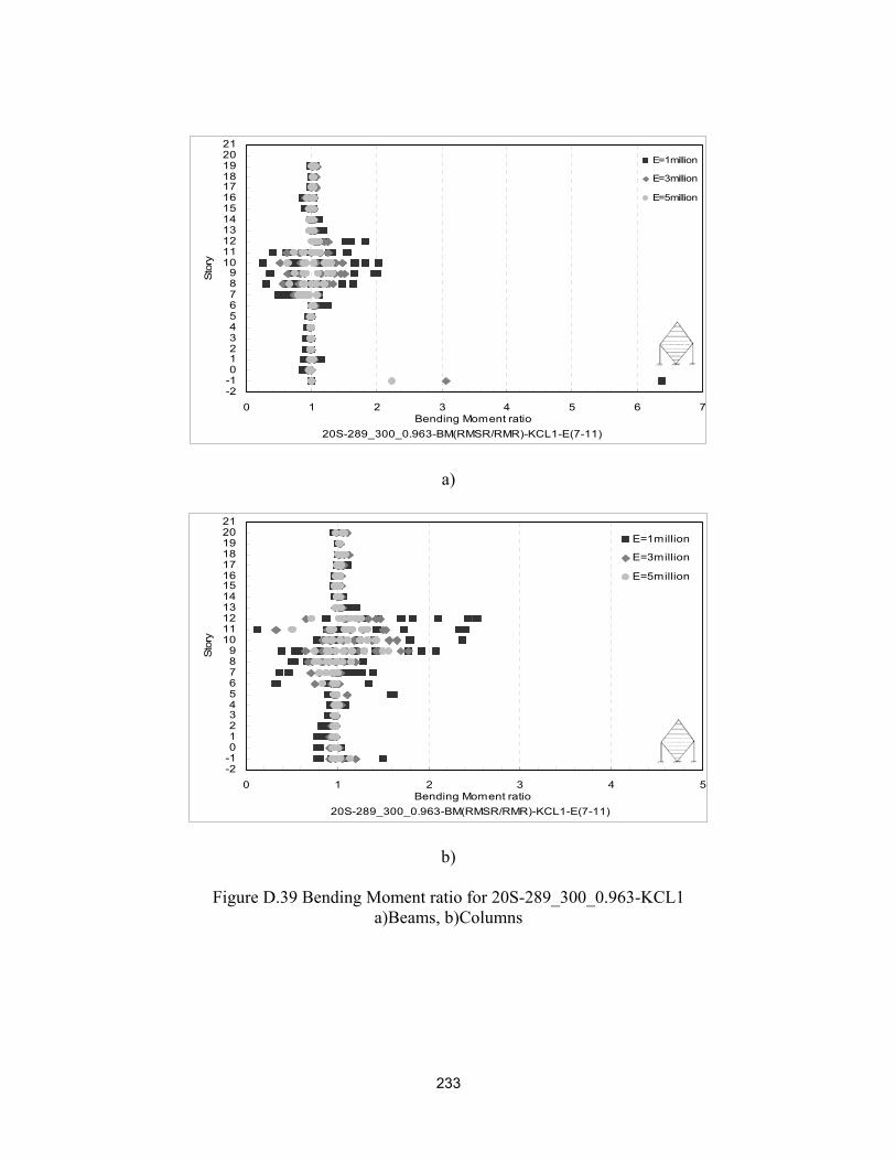
233
-2-10123456789
101112131415161718192021
0 1 2 3 4 5 6 7Bending Moment ratio
Sto
ry
E=1million
E=3million
E=5million
20S-289_300_0.963-BM(RMSR/RMR)-KCL1-E(7-11)
a)
-2-10123456789
101112131415161718192021
0 1 2 3 4 5Bending Moment ratio
Stor
y
E=1million
E=3million
E=5million
20S-289_300_0.963-BM(RMSR/RMR)-KCL1-E(7-11)
b)
Figure D.39 Bending Moment ratio for 20S-289_300_0.963-KCL1 a)Beams, b)Columns
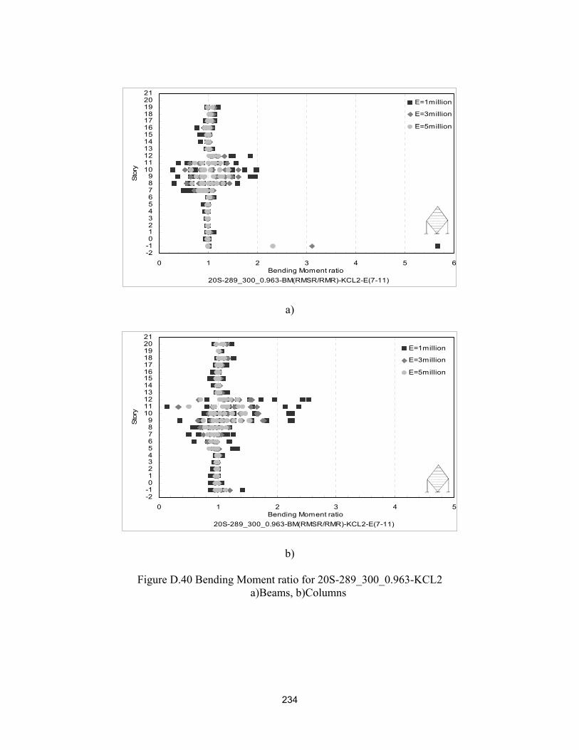
234
-2-10123456789
101112131415161718192021
0 1 2 3 4 5 6Bending Moment ratio
Sto
ry
E=1million
E=3million
E=5million
20S-289_300_0.963-BM(RMSR/RMR)-KCL2-E(7-11)
a)
-2-10123456789
101112131415161718192021
0 1 2 3 4 5Bending Moment ratio
Stor
y
E=1million
E=3million
E=5million
20S-289_300_0.963-BM(RMSR/RMR)-KCL2-E(7-11)
b)
Figure D.40 Bending Moment ratio for 20S-289_300_0.963-KCL2 a)Beams, b)Columns

235
APPENDIX E
MAXIMUM LATERAL DISPLACEMENT PROFILE

236
0
1
2
3
4
0 2 4 6 8Maximum Displacement-Ux(inch)
Stor
y
0 5 10 15 20Maximum Displacement-Ux(cm)
3S-39_120_0.325-MDUx(RMR)-PKF 3S-39_120_0.325-MDUx(RCR)-PKF
.
Figure E.1 Maximum lateral displacement for 3S-39_120_0.325-PKF
0
1
2
3
4
0 1 2 3 4Maximum Displacement-Ux(inch)
Stor
y
0 2.5 5 7.5 10Maximum Displacement-Ux(cm)
3S-39_120_0.325-MDUx(RMR)-ELC 3S-39_120_0.325-MDUx(RCR)-ELC
.
Figure E.2 Maximum lateral displacement for 3S-39_120_0.325-ELC

237
0
1
2
3
4
0 1 2 3 4 5Maximum Displacement-Ux(inch)
Stor
y
0 2.5 5 7.5 10 12.5Maximum Displacement-Ux(cm)
3S-39_120_0.325-MDUx(RMR)-NRG 3S-39_120_0.325-MDUx(RCR)-NRG
.
Figure E.3 Maximum lateral displacement for 3S-39_120_0.325-NRG
0
1
2
3
4
0 0.03 0.06 0.09 0.12 0.15Maximum Displacement-Ux(inch)
Stor
y
0 0.07 0.14 0.21 0.28 0.35Maximum Displacement-Ux(cm)
3S-39_120_0.325-MDUx(RMR)-KCL1 3S-39_120_0.325-MDUx(RCR)-KCL1
.
Figure E.4 Maximum lateral displacement for 3S-39_120_0.325-KCL1

238
0
1
2
3
4
0 0.01 0.02 0.03 0.04 0.05Maximum Displacement-Ux(inch)
Stor
y
0 0.03 0.06 0.09 0.12Maximum Displacement-Ux(cm)
3S-39_120_0.325-MDUx(RMR)-KCL2 3S-39_120_0.325-MDUx(RCR)-KCL2
.
Figure E.5 Maximum lateral displacement for 3S-39_120_0.325-KCL2
0
1
2
3
4
5
6
7
8
9
0 2 4 6 8 10 12 14 16 18 20Maximum Displacement-Ux(inch)
Stor
y
0 5 10 15 20 25 30 35 40 45 50
Maximum Displacement-Ux(cm)
9S-134_150_0.893-MDUx(RMR)-PKF 9S-134_150_0.893-MDUx(RCR)-PKF
Figure E.6 Maximum lateral displacement for 9S-134_150_0.893-PKF

239
0
1
2
3
4
5
6
7
8
9
0 2 4 6 8 10Maximum Displacement-Ux(inch)
Stor
y
0 5 10 15 20 25
Maximum Displacement-Ux(cm)
9S-134_150_0.893-MDUx(RMR)-ELC 9S-134_150_0.893-MDUx(RCR)-ELC
Figure E.7 Maximum lateral displacement for 9S-134_150_0.893-ELC
0
1
2
3
4
5
6
7
8
9
0 5 10 15 20 25Maximum Displacement-Ux(inch)
Stor
y
0 12 24 36 48 60Maximum Displacement-Ux(cm)
9S-134_150_0.893-MDUx(RMR)-NRG 9S-134_150_0.893-MDUx(RCR)-NRG
.
Figure E.8 Maximum lateral displacement for 9S-134_150_0.893-NRG

240
0
1
2
3
4
5
6
7
8
9
0 0.15 0.3 0.45 0.6 0.75Maximum Displacement-Ux(inch)
Stor
y
0 0.4 0.8 1.2 1.6Maximum Displacement-Ux(cm)
9S-134_150_0.893-MDUx(RMR)-KCL1 9S-134_150_0.893-MDUx(RCR)-KCL1
.
Figure E.9 Maximum lateral displacement for 9S-134_150_0.893-KCL1
0
1
2
3
4
5
6
7
8
9
0 0.15 0.3 0.45 0.6 0.75Maximum Displacement-Ux(inch)
Stor
y
0 0.4 0.8 1.2 1.6Maximum Displacement-Ux(cm)
9S-134_150_0.893-MDUx(RMR)-KCL2 9S-134_150_0.893-MDUx(RCR)-KCL2
.
Figure E.10 Maximum lateral displacement for 9S-134_150_0.893-KCL2

241
-1
0
1
2
3
4
5
6
7
8
9
10
11
12
0 5 10 15 20Maximum Displacement-Ux(inch)
Stor
y
0 10 20 30 40 50Maximum Displacement-Ux(cm)
12S-173_150_1.153-MDUx(RMR)-PKF 12S-173_150_1.153-MDUx(RCR)-PKF
Figure E.11 Maximum lateral displacement for 12S-173_150_1.153-PKF
-1
0
1
2
3
4
5
6
7
8
9
10
11
12
0 3 6 9 12 15Maximum Displacement-Ux(inch)
Stor
y
0 7 14 21 28 35Maximum Displacement-Ux(cm)
12S-173_150_1.153-MDUx(RMR)-ELC 12S-173_150_1.153-MDUx(RCR)-ELC
Figure E.12 Maximum lateral displacement for 12S-173_150_1.153-ELC

242
-1
0
1
2
3
4
5
6
7
8
9
10
11
12
0 8 16 24 32 40Maximum Displacement-Ux(inch)
Stor
y
0 20 40 60 80 100Maximum Displacement-Ux(cm)
12S-173_150_1.153-MDUx(RMR)-NRG 12S-173_150_1.153-MDUx(RCR)-NRG
.
Figure E.13 Maximum lateral displacement for 12S-173_150_1.153-NRG
-1
0
1
2
3
4
5
6
7
8
9
10
11
12
0 0.15 0.3 0.45 0.6 0.75Maximum Displacement-Ux(inch)
Stor
y
0 0.4 0.8 1.2 1.6Maximum Displacement-Ux(cm)
12S-173_150_1.153-MDUx(RMR)-KCL1 12S-173_150_1.153-MDUx(RCR)-KCL1
.
Figure E.14 Maximum lateral displacement for 12S-173_150_1.153-KCL1

243
-1
0
1
2
3
4
5
6
7
8
9
10
11
12
0 0.25 0.5 0.75 1 1.25Maximum Displacement-Ux(inch)
Stor
y
0 0.6 1.2 1.8 2.4 3Maximum Displacement-Ux(cm)
12S-173_150_1.153-MDUx(RMR)-KCL2 12S-173_150_1.153-MDUx(RCR)-KCL2
.
Figure E.15 Maximum lateral displacement for 12S-173_150_1.153-KCL2
-2-10123456789
1011121314151617181920
0 5 10 15 20 25Maximum Displacement-Ux(inch)
Stor
y
0 10 20 30 40 50 60Maximum Displacement-Ux(cm)
20S-289_100_2.89-MDUx(RMR)-PKF 20S-289_100_2.89-MDUx(RCR)-PKF
Figure E.16 Maximum lateral displacement for 20S-289_100_2.89-PKF

244
-2-10123456789
1011121314151617181920
0 3 6 9 12 15 18Maximum Displacement-Ux(inch)
Stor
y
0 7 14 21 28 35 42 49Maximum Displacement-Ux(cm)
20S-289_100_2.89-MDUx(RMR)-ELC 20S-289_100_2.89-MDUx(RCR)-ELC
Figure E.17 Maximum lateral displacement for 20S-289_100_2.89-ELC
-2-10123456789
1011121314151617181920
0 8 16 24 32 40Maximum Displacement-Ux(inch)
Stor
y
0 20 40 60 80 100Maximum Displacement-Ux(cm)
20S-289_100_2.89-MDUx(RMR)-NRG 20S-289_100_2.89-MDUx(RCR)-NRG
.
Figure E.18 Maximum lateral displacement for 20S-289_100_2.89-NRG

245
-2-10123456789
1011121314151617181920
0 0.2 0.4 0.6 0.8 1Maximum Displacement-Ux(inch)
Stor
y
0 0.5 1 1.5 2 2.5Maximum Displacement-Ux(cm)
20S-289_100_2.89-MDUx(RMR)-KCL1 20S-289_100_2.89-MDUx(RCR)-KCL1
.
Figure E.19 Maximum lateral displacement for 20S-289_100_2.89-KCL1
-2-10123456789
1011121314151617181920
0 0.25 0.5 0.75 1 1.25 1.5 1.75Maximum Displacement-Ux(inch)
Stor
y
0 0.9 1.8 2.7 3.6Maximum Displacement-Ux(cm)
20S-289_100_2.89-MDUx(RMR)-KCL2 20S-289_100_2.89-MDUx(RCR)-KCL2
.
Figure E.20 Maximum lateral displacement for 20S-289_100_2.89-KCL2

246
-2-10123456789
1011121314151617181920
0 5 10 15 20 25Maximum Displacement-Ux(inch)
Sto
ry
0 10 20 30 40 50 60Maximum Displacement-Ux(cm)
Rigid
Semi-rigid, E=1million
Semi-rigid, E=3millionSemi-rigid, E=5million
20S-289_100_2.89-MDux-PKF-E(7-11)
Figure E.21 Maximum lateral displacement for 20S-289_100_2.89-PKF
-2-10123456789
1011121314151617181920
0 5 10 15 20Maximum Displacement-Ux(inch)
Sto
ry
0 10 20 30 40 50Maximum Displacement-Ux(cm)
Rigid
Semi-rigid, E=1million
Semi-rigid, E=3millionSemi-rigid, E=5million
20S-289_100_2.89-MDux-ELC-E(7-11)
Figure E.22 Maximum lateral displacement for 20S-289_100_2.89-ELC

247
-2-10123456789
1011121314151617181920
0 5 10 15 20 25 30 35 40Maximum Displacement-Ux(inch)
Sto
ry
0 20 40 60 80 100Maximum Displacement-Ux(cm)
RigidSemi-rigid, E=1millionSemi-rigid, E=3millionSemi-rigid, E=5million
20S-289_100_2.89-MDux-NRG-E(7-11)
Figure E.23 Maximum lateral displacement for 20S-289_100_2.89-NRG
-2-10123456789
1011121314151617181920
0 0.25 0.5 0.75 1 1.25Maximum Displacement-Ux(inch)
Sto
ry
0 0.5 1 1.5 2 2.5 3Maximum Displacement-Ux(cm)
Rigid
Semi-rigid, E=1million
Semi-rigid, E=3millionSemi-rigid, E=5million
20S-289_100_2.89-MDux-KCL1-E(7-11)
Figure E.24 Maximum lateral displacement for 20S-289_100_2.89-KCL1

248
-2-10123456789
1011121314151617181920
0 0.25 0.5 0.75 1 1.25 1.5 1.75Maximum Displacement-Ux(inch)
Sto
ry
0 0.9 1.8 2.7 3.6Maximum Displacement-Ux(cm)
Rigid
Semi-rigid, E=1million
Semi-rigid, E=3millionSemi-rigid, E=5million
20S-289_100_2.89-MDux-KCL2-E(7-11)
Figure E.25 Maximum lateral displacement for 20S-289_100_2.89-KCL2
-2-10123456789
1011121314151617181920
0 5 10 15 20Maximum Displacement-Ux(inch)
Sto
ry
0 10 20 30 40 50Maximum Displacement-Ux(cm)
Rigid
Semi-rigid, E=1million
Semi-rigid, E=3millionSemi-rigid, E=5million
20S-289_100_2.89-MDux-PKF-E(7-11)
Figure E.26 Maximum lateral displacement for 20S-289_100_2.89-PKF

249
-2-10123456789
1011121314151617181920
0 2 4 6 8Maximum Displacement-Ux(inch)
Sto
ry
0 5 10 15 20Maximum Displacement-Ux(cm)
Rigid
Semi-rigid, E=1million
Semi-rigid, E=3millionSemi-rigid, E=5million
20S-289_100_2.89-MDux-ELC-E(7-11)
Figure E.27 Maximum lateral displacement for 20S-289_100_2.89-ELC
-2-10123456789
1011121314151617181920
0 2 4 6 8 10 12 14 16Maximum Displacement-Ux(inch)
Sto
ry
0 5 10 15 20 25 30 35 40Maximum Displacement-Ux(cm)
Rigid
Semi-rigid, E=1million
Semi-rigid, E=3millionSemi-rigid, E=5million
20S-289_100_2.89-MDux-NRG-E(7-11)
Figure E.28 Maximum lateral displacement for 20S-289_100_2.89-NRG

250
-2-10123456789
1011121314151617181920
0 0.15 0.3 0.45 0.6 0.75Maximum Displacement-Ux(inch)
Sto
ry
0 0.4 0.8 1.2 1.6Maximum Displacement-Ux(cm)
Rigid
Semi-rigid, E=1million
Semi-rigid, E=3millionSemi-rigid, E=5million
20S-289_100_2.89-MDux-KCL1-E(7-11)
Figure E.29 Maximum lateral displacement for 20S-289_100_2.89-KCL1
-2-10123456789
1011121314151617181920
0 0.15 0.3 0.45 0.6 0.75Maximum Displacement-Ux(inch)
Sto
ry
0 0.4 0.8 1.2 1.6Maximum Displacement-Ux(cm)
Rigid
Semi-rigid, E=1million
Semi-rigid, E=3millionSemi-rigid, E=5million
20S-289_100_2.89-MDux-KCL2-E(7-11)
Figure E.30 Maximum lateral displacement for 20S-289_100_2.89-KCL2

251
APPENDIX F
LATERAL INTER STORY DRIFT

252
0
1
2
3
4
0 0.004 0.008 0.012 0.016 0.02Lateral Drift
Sto
ry
Lateral Drift for Rhombus Frame Lateral Drift for Rectangular Frame
.
Figure F.1 Inter Story Drift for 3S-39_120_0.325-PKF
0
1
2
3
4
0 0.004 0.008 0.012 0.016 0.02Lateral Drift
Sto
ry
Lateral Drift for Rhombus Frame Lateral Drift for Rectangular Frame
.
Figure F.2 Inter Story Drift for 3S-39_120_0.325-ELC

253
0
1
2
3
4
0 0.004 0.008 0.012 0.016 0.02Lateral Drift
Sto
ry
Lateral Drift for Rhombus Frame Lateral Drift for Rectangular Frame
.
Figure F.3 Inter Story Drift for 3S-39_120_0.325-NRG
0
1
2
3
4
0 0.0001 0.0002 0.0003 0.0004 0.0005Lateral Drift
Sto
ry
Lateral Drift for Rhombus Frame Lateral Drift for Rectangular Frame
.
Figure F.4 Inter Story Drift for 3S-39_120_0.325-KCL1

254
0
1
2
3
4
0 0.00004 0.00008 0.00012 0.00016 0.0002Lateral Drift
Sto
ry
Lateral Drift for Rhombus Frame Lateral Drift for Rectangular Frame
.
Figure F.5 Inter Story Drift for 3S-39_120_0.325-KCL2
0
1
2
3
4
5
6
7
8
9
0 0.005 0.01 0.015 0.02 0.025 0.03Lateral Drift
Sto
ry
Lateral Drift for Rhombus Frame Lateral Drift for Rectangular Frame
.
Figure F.6 Inter Story Drift for 9S-134_150_0.893-PKF

255
0
1
2
3
4
5
6
7
8
9
0 0.002 0.004 0.006 0.008 0.01Lateral Drift
Sto
ry
Lateral Drift for Rhombus Frame Lateral Drift for Rectangular Frame
.
Figure F.7 Inter Story Drift for 9S-134_150_0.893-ELC
0
1
2
3
4
5
6
7
8
9
0 0.005 0.01 0.015 0.02 0.025 0.03Lateral Drift
Sto
ry
Lateral Drift for Rhombus Frame Lateral Drift for Rectangular Frame
.
Figure F.8 Inter Story Drift for 9S-134_150_0.893-NRG

256
0
1
2
3
4
5
6
7
8
9
0 0.0002 0.0004 0.0006 0.0008 0.001Lateral Drift
Sto
ry
Lateral Drift for Rhombus Frame Lateral Drift for Rectangular Frame
.
Figure F.9 Inter Story Drift for 9S-134_150_0.893-KCL1
0
1
2
3
4
5
6
7
8
9
0 0.0002 0.0004 0.0006 0.0008 0.001Lateral Drift
Sto
ry
Lateral Drift for Rhombus Frame Lateral Drift for Rectangular Frame
.
Figure F.10 Inter Story Drift for 9S-134_150_0.893-KCL2

257
0
1
2
3
4
5
6
7
8
9
10
11
12
0 0.01 0.02 0.03Lateral Drift
Sto
ry
Lateral Drift for Rhombus Frame Lateral Drift for Rectangular Frame
.
Figure F.11 Inter Story Drift for 12S-173_150_1.153-PKF
0
1
2
3
4
5
6
7
8
9
10
11
12
0 0.01 0.02 0.03Lateral Drift
Sto
ry
Lateral Drift for Rhombus Frame Lateral Drift for Rectangular Frame
.
Figure F.12 Inter Story Drift for 12S-173_150_1.153-ELC

258
0
1
2
3
4
5
6
7
8
9
10
11
12
0 0.01 0.02 0.03 0.04Lateral Drift
Sto
ry
Lateral Drift for Rhombus Frame Lateral Drift for Rectangular Frame
.
Figure F.13 Inter Story Drift for 12S-173_150_1.153-NRG
0
1
2
3
4
5
6
7
8
9
10
11
12
0 0.0002 0.0004 0.0006 0.0008 0.001Lateral Drift
Sto
ry
Lateral Drift for Rhombus Frame Lateral Drift for Rectangular Frame
.
Figure F.14 Inter Story Drift for 12S-173_150_1.153-KCL1

259
0
1
2
3
4
5
6
7
8
9
10
11
12
0 0.0003 0.0006 0.0009 0.0012Lateral Drift
Sto
ry
Lateral Drift for Rhombus Frame Lateral Drift for Rectangular Frame
.
Figure F.15 Inter Story Drift for 12S-173_150_1.153-KCL2
0123456789
1011121314151617181920
0 0.004 0.008 0.012 0.016 0.02Lateral Drift
Sto
ry
Lateral Drift for Rhombus Frame Lateral Drift for Rectangular Frame
.
Figure F.16 Inter Story Drift for 20S-289_100_2.89-PKF

260
0123456789
1011121314151617181920
0 0.003 0.006 0.009 0.012 0.015Lateral Drift
Sto
ry
Lateral Drift for Rhombus Frame Lateral Drift for Rectangular Frame
.
Figure F.17 Inter Story Drift for 20S-289_100_2.89-ELC
0123456789
1011121314151617181920
0 0.005 0.01 0.015 0.02 0.025Lateral Drift
Sto
ry
Lateral Drift for Rhombus Frame Lateral Drift for Rectangular Frame
.
Figure F.18 Inter Story Drift for 20S-289_100_2.89-NRG

261
0123456789
1011121314151617181920
0 0.0002 0.0004 0.0006 0.0008 0.001Lateral Drift
Sto
ry
Lateral Drift for Rhombus Frame Lateral Drift for Rectangular Frame
.
Figure F.19 Inter Story Drift for 20S-289_100_2.89-KCL1
0123456789
1011121314151617181920
0 0.0002 0.0004 0.0006 0.0008 0.001Lateral Drift
Sto
ry
Lateral Drift for Rhombus Frame Lateral Drift for Rectangular Frame
.
Figure F.20 Inter Story Drift for 20S-289_100_2.89-KCL2

262
0123456789
1011121314151617181920
0 0.004 0.008 0.012 0.016 0.02Lateral Drift
Sto
ry
RigidSemi-rigid,E=1millionSemi-rigid, E=3millionSemi-rigid, E=5million
.
20S-289_100_2.89-LDr-PKF-E(7-11)
Figure F.21 Inter Story Drift for 20S-289_100_2.89-PKF
0123456789
1011121314151617181920
0 0.004 0.008 0.012 0.016 0.02Lateral Drift
Sto
ry
RigidSemi-rigid,E=1millionSemi-rigid, E=3millionSemi-rigid, E=5million
.
20S-289_100_2.89-LDr-ELC-E(7-11)
Figure F.22 Inter Story Drift for 20S-289_100_2.89-ELC

263
0123456789
1011121314151617181920
0 0.004 0.008 0.012 0.016 0.02Lateral Drift
Sto
ry
RigidSemi-rigid,E=1millionSemi-rigid, E=3millionSemi-rigid, E=5million
.
20S-289_100_2.89-LDr-NRG-E(7-11)
Figure F.23 Inter Story Drift for 20S-289_100_2.89-NRG
0123456789
1011121314151617181920
0 0.0002 0.0004 0.0006 0.0008 0.001Lateral Drift
Sto
ry
RigidSemi-rigid,E=1millionSemi-rigid, E=3millionSemi-rigid, E=5million
.
20S-289_100_2.89-LDr-KCL1-E(7-11)
Figure F.24 Inter Story Drift for 20S-289_100_2.89-KCL1

264
0123456789
1011121314151617181920
0 0.0002 0.0004 0.0006 0.0008 0.001Lateral Drift
Sto
ry
RigidSemi-rigid,E=1millionSemi-rigid, E=3millionSemi-rigid, E=5million
.
20S-289_100_2.89-LDr-KCL2-E(7-11)
Figure F.25 Inter Story Drift for 20S-289_100_2.89-KCL2
0123456789
1011121314151617181920
0 0.004 0.008 0.012 0.016 0.02Lateral Drift
Sto
ry
RigidSemi-rigid,E=1millionSemi-rigid, E=3millionSemi-rigid, E=5million
.
20S-289_100_2.89-LDr-PKF-E(7-11)
Figure F.26 Inter Story Drift for 20S-289_100_2.89-PKF

265
0123456789
1011121314151617181920
0 0.002 0.004 0.006 0.008 0.01Lateral Drift
Sto
ry
RigidSemi-rigid,E=1millionSemi-rigid, E=3millionSemi-rigid, E=5million
.
20S-289_100_2.89-LDr-ELC-E(7-11)
Figure F.27 Inter Story Drift for 20S-289_100_2.89-ELC
0123456789
1011121314151617181920
0 0.004 0.008 0.012 0.016 0.02Lateral Drift
Sto
ry
RigidSemi-rigid,E=1millionSemi-rigid, E=3millionSemi-rigid, E=5million
.
20S-289_100_2.89-LDr-NRG-E(7-11)
Figure F.28 Inter Story Drift for 20S-289_100_2.89-NRG

266
0123456789
1011121314151617181920
0 0.0002 0.0004 0.0006 0.0008Lateral Drift
Sto
ry
RigidSemi-rigid,E=1millionSemi-rigid, E=3millionSemi-rigid, E=5million
.
20S-289_100_2.89-LDr-KCL1-E(7-11)
Figure F.29 Inter Story Drift for 20S-289_100_2.89-KCL1
0123456789
1011121314151617181920
0 0.0002 0.0004 0.0006 0.0008Lateral Drift
Sto
ry
RigidSemi-rigid,E=1millionSemi-rigid, E=3millionSemi-rigid, E=5million
.
20S-289_100_2.89-LDr-KCL2-E(7-11)
Figure F.30 Inter Story Drift for 20S-289_100_2.89-KCL2

267
APPENDIX G
LOAD CALCULATION

268
Load calculations for this study follow ASCE (American Society of Civil
Engineers) standards. For dead load, a 4 inch slab thickness is considered with a super
imposed dead load of 30 psf. Other dead loads are considered as per Table C3-1, ASCE
7-05.
Self weight of slab = 50 psf
Super imposed dead load = 40 psf
Mechanical duct allowance = 4 psf (Table C3-1, ASCE 7-05)
Plaster = 5 psf (Table C3-1, ASCE 7-05)
Floor finish = 32 psf (Table C3-1, ASCE 7-05)
Exterior stud walls = 48 psf (Table C3-1, ASCE 7-05)
i.e. Total dead load = 179 ≈ 180 psf
For live load calculation, residential building is considered. As per Section 4.2.2
of the ASCE 7-05, 30 psf live load for partition wall is considered. Minimum distributed
live load for residential building is 40 psf as per Table 4-1, ASCE 7-05.
i.e. Total live load = 70 psf.
For effective seismic load, total dead load and 25 percentage of live load are
considered as per Section 12.7.2, ASCE 7-05.

269
i.e. total effective seismic load = 180 + 0.25 X 70 = 197.5 psf. This load will contribute to
the mass source.
For, 20- story three dimensional building; each slab dimension is 20 ft by 20 ft.
For each beam, tributary area is equal to 100 ft2, which leads to a uniformly distributed
load on all beams = ftkip /9875.0100020
1005.197=
×× . Other tributary area will contribute to
the point load at beam ends.
Point loads for outer nodes = kip875.92
209875.0=
×
Point loads for inner nodes = 19.75 kip
For 3-, 9-, 12- story three dimensional buildings, each slab dimension is 30 ft by
30 ft. For each beam, tributary area is equal to 225 ft2, which leads to an uniformly
distributed load = ftkip /481.1100020
2255.197=
×× .
Point loads for outer nodes = kip215.222
30481.1=
×
Point loads for inner nodes = 44.43 kip

270
REFERENCES
Abolmaali, Ali, Ardavan Motahari, and Mehdi Ghassemieh. "Energy Dissipation
Characteristics of Semi-Rigid Connections." Journal of Construction
Steel Research (2008).
AISC. 2005a. ANSI/AISC 341-05: Seismic Provisions for Structural Steel Buildings.
Chicago: American Institute of Steel Construction.
Al-Mashary, F. and Chen, W.F., “Simplified second-order inelastic analysis for steel
frames.” Structural Engineer, (1991): 69(23), 395-399.
ASCE. 2005. SEI/ASCE 7-05: Minimum Design Loads for Buildings and Other
Structures. Reston, VA: American Society of Civil Engineers.
ATC, 1997a, NEHRP Guidelines for the Seismic Rehabilitation of Buildings, FEMA-273,
prepared by the Applied Technology Council, Redwood City, California, for the
Building Seismic Safety Council, published by the Federal Emergency
Management Agency, Washington, DC.
ATC, 1997b, NEHRP Commentary on the Guidelines for the Seismic Rehabilitation of
Buildings, FEMA-274, prepared by the Applied Technology Council, Redwood
City, California, for the Building Seismic Safety Council, published by the
Federal Emergency Management Agency, Washington, DC.

271
ATC, 1992, Development of Guidelines for Seismic Rehabilitation of Buildings, Phase I:
Issues Identification and Resolution, developed by the Applied Technology
Council (Report No. ATC-28) for the Federal Emergency Management Agency
(Report No. FEMA 237), Washington, D.C.
Bhatti, M. A., Hingtgen, James D., “Effects of Connection Stiffness and Plasticity on the
Service Load Behavior of Unbraced Steel Frames.” Engineering Journal, First
quarter (1995): 21-33.
Bonowitz, D., “SAC Database of WSMF Connection Tests.” Contractor’s report
submitted to the SAC Joint Venture,1999(a).
Bruneau, Michel, Uang, Chia-Ming, Whittaker. Andrew, Ductile Design of Steel
Structures engineering. McGraw-Hill, 1998.
Chan, S.L., Chui, P.P.T., Non-Linear Static and Cyclic Analysis of Steel Frames with
Semi-Rigid Connections, Elsevier, Netherlands, 2000.
Chen, W.F., Lui, E.M., Stability Design of Steel Frames. CRC Press, Boca Raton, FL
1991.
Chopra, Anil K., Dynamics of structures theory and applications to earthquake
engineering. Ed. Prentice Hall. 3rd ed. Upper Saddle River, N.J: Pearson/Prentice
Hall, 2007.
Engelhardt, M.D., and Husain, A.S, “Cyclic Loading Performance of Welded Flange-
Bolted Web Connections.” Journal of Structural Engineering, American Society
of Civil Engineers, (1993): Vol. 119, No. 12: 3537-3550.

272
FEMA-273, 1997a, NEHRP Guidelines for the Seismic Rehabilitation of Buildings,
prepared by the Applied Technology Council, Redwood City, California, for the
Building Seismic Safety Council, published by the Federal Emergency
Management Agency, Washington, DC.
FEMA-355C, 2000, State of the Art Report on Systems Performance of Steel Moment
Frames Subject to Earthquake Ground Shaking, prepared by the SAC Joint
Venture for the Federal Emergency Management Agency, Washington, DC.
FEMA-355D, 2000, State of the Art Report on Connection Performance, prepared by the
SAC Joint Venture for the Federal Emergency Management Agency, Washington,
DC.
FEMA-355E, 2000, State of the Art Report on Past Performance of Steel Moment-Frame
Buildings in Earthquakes, prepared by the SAC Joint Venture for the Federal
Emergency Management Agency, Washington, DC.
FEMA-355F, 2000, State of the Art Report on Performance Prediction and Evaluation of
Steel Moment-Frame Buildings, prepared by the SAC Joint Venture for the
Federal Emergency Management Agency, Washington, DC.
FEMA-356, 2000, Prestandard and Commentary for the Seismic Rehabilitation of
Buildings, prepared by American Society of Civil Engineers for the Federal
Emergency Management Agency, Washington, DC.
Goel, Subhash C., Chao, Shih-Ho, Performance-Based Plastic Design Earthquake
Resistant Steel Structures, International Code Council, 2008.

273
Maison, B.F., and K. Kasai, “Seismic Performance of 3 and 9 Story Partially Restrained
Moment Frame Buildings,” SAC/BD-99/16, (1999).
Newmark, N.M., “A Method of Computation for Structural Dynamics,” Journal of the
Engineering Mechanics Division, ASCE, 85 (1959): pp. 67-94.
Open System for Earthquake Engineering Simulation - Home Page. Web. 1 Feb. 2008.
<http://opensees.berkeley.edu/index.php>.
"PEER Strong Motion Database: Introduction." Welcome to Pacific Earthquake
Engineering Research Center - PEER. Web. 15 Mar. 2008.
<http://peer.berkeley.edu/smcat/>.
Popov, E.P., and Pinkney, R.B., “Cyclic Yield Reversals on Steel Building Connections,”
Journal of the Structural Division, ASCE, (1969): Vol. 95, No. 3.
Popov, E.P., and Stephen, RM., “Cyclic Loading of Full-Size Steel Connections.”
Earthquake Engineering Research Center Report UCB/EERC-70-3,
University of California, Berkeley, 1970.
Popov, E.P., and Stephen, RM, “Cyclic Loading of Full-Size Steel Connections.”
American Iron and Steel Institute. Bulletin No. 21. New York, 1972.
Popov, E.P., Amin, N.R., Louie, J.J.C., and Stephen, R.M., “Cyclic Behavior of
LargeBeam-Column Assemblies,” Earthquake Spectra, Earthquake Engineering
Research Institute, (1985).
Radulova, Dobrinka, Nonlinear Dynamic Analysis of Hybrid Frames, Masters Thesis,
Department of Civil Engineering, The University of Texas at Arlington,
Arlington, Texas, 2009.

274
Roeder, C.W., and Foutch, D.A., “Experimental Results for Seismic Resistant Steel
Moment Frame Connections.” Journal of Structural Engineering. American
Society of Civil Engineers, (1995): Vol. 122, No.6: 581-588.
Roeder, C.W. and Foutch, D.A., “Experimental Results for Seismic Resistant Steel
Moment Frame Connections,” Journal of Structural Engineering. (1996).
Sabelli, R., FEMA/EERI report: “ Research on Improving the Design and Analysis of
Earthquake Resistant Steel Braced Frames.” Washington, D.C.,2000:
FEMA/EERI
SAC, 1995, Interim Guidelines, Inspection, Evaluation, Repair, Upgrade and Design of
Welded Moment Resisting Steel Structures, FEMA-267, prepared by the SAC
Joint Venture for the Federal Emergency Management Agency, Washington, DC.
Superseded b FEMA 350.
SEAOC Vision 2000 Committee, 1995, A Framework for Performance Based Design,
Volumes I, II, and III, Structural Engineers Association of California (SEAOC),
Sacramento, California.
"SeismoSoft - SeismoSignal." SeismoSoft - Home. Web. 27 Aug. 2009.
<http://www.seismosoft.com/en/SeismoSignal.aspx>.
Steel Construction Manual, 13th Edition (Book). New York: American Institute of Steel
Construction, 2006.
Structural Analysis Program, SAP2000, Advanced 11.0.2, Computers and Structures,
Inc., Berkeley CA.

275
Tsai, K.C. and Popov, E.P., “Steel Beam-Column Joints in Seismic Moment Resisting
Frames.” (UCB/EERC-88/19), Earthquake Engineering Research Center,
Richmond, California, 1988.
Yau, C.Y. and Chan, S.L., “Inelastic and stability analysis of flexibly connected steel
frames by springs-in-series model.” Journal of Structural Engineering.
American Society of Civil Engineers, (1994): Vol. 120, No. 10 : 2803-2819.
276
BIOGRAPHICAL INFORMATION
S. M. Ashfaqul Hoq was born on 23rd May, 1984 in Dhaka, Bangladesh. He
received his Bachelor’s degree in Civil Engineering from Bangladesh University of
Engineering and Technology, Dhaka, Bangladesh in June 2007. After his graduation, he
started working in “Dalan-Kotha Limited”, a construction firm. He worked as a Project
Engineer from July 2007 to June 2008. His job responsibilities include supervision and
management of different construction projects, mainly for apartment complex. Later on,
Hoq started his graduate studies at the University of Texas at Arlington in Fall 2008. He
was awarded with the prestigious Graduate Dean Masters Fellowship scholarship. The
author worked under the guidance of Dr. Ali Abolmaali to propose a frame shape, which
will improve building performance under earthquake excitations. His Masters thesis is
substantially based on this research work.