1

Effect of Forecast Accuracy on Inventory Optimization Model

Surya Gundavarapu, Prasad Gujela, Shan Lin, Matthew A. Lanham

Purdue University, Department of Management, 403 W. State Street, West Lafayette, IN 47907

sgundava@purdue.edu; pgujela@purdue.edu; lin882@purdue.edu; lanhamm@purdue.edu

Abstract

In this study, we examine the effect of forecast accuracy on the inventory costs incurred by a national

retailer using a dynamic inventory optimization model. In the past, the retailer calculated weekly and

monthly demand forecasts at a particular distribution center by dividing the annual demand with

specific numbers which led to a consistently flat ordering model. This led the retailer to purchase

items in bulk from their vendors which led to incurring unnecessary holding costs. The motivation

for study is that this type of purchase behavior does not adequately prepare a supply chain for

unexpected demand and thus might further deepen their inventory troubles. We introduced to this

retailer an easy to deploy inventory model that uses the distribution of demand for each item along

with the target service level among other constraints like the purchase capacity etc., to minimize the

overall cost for each item. We then show the impact of inventory costs based on how accurate the

demand forecast is.

Keywords: Dynamic Inventory Optimization, Forecast Accuracy, Wagner-Whitin Algorithm

2

Introduction

Companies use inventory as a buffer between supply and demand volatility. Handling optimal

inventory level is important for retailers since too much inventory would imply too much capital

struck in the supply chain, while too little inventory would prevent customer fulfillment to a

satisfactory level. Further, mishandling inventory would not just affect the supply chain department

but the overall KPIs of the firm.

Nowadays, large firms use ERP systems to aid them in their inventory decisions and these ERP

systems integrate critical information about the supply chain, such as customer orders, warehouse

capabilities, and demand forecasts to help managers make informed decisions (Fritsch,2017). Further,

today firms are investing heavily into machine learning, Big Data Analytics, and the Internet of

Things to bring more analytic power to operational decision support systems. For instance, a

warehouse manager can now incorporate images as data inputs for intelligent stock management

systems that can predict when the company should re-order (Marr, 2016).

By improving demand accuracy, companies can reduce the safety stock and free up more cash for

other areas of the business. For business-to-consumer (B2C) supply chains, for example, a consumer

goods company will forecast what stock keeping units a retailer will order. Also, demand

management teams must collaborate with sales forces to accurately estimate the probability that a

deal will close and what products the deal will include (Banker, 2013). Therefore, a company could

reduce the inventory per square foot and turnover days to keep the cash flow.

Unfortunately, improving the demand forecasts is not enough. What really matters is how the

company implements stocking and reorder points. In practice, other factors should be incorporated

into the process design such as transportation costs. Recently, a Dutch adult beverage firm

successfully reduced its freight cost by implementing dynamic order allocation which integrates

customer order information and available stock levels. With more information, the company can make

strategic decisions in optimizing cost while maximizing customer fulfillment (Banker, 2015).

Our research question in this study is, how does demand forecast accuracy translate to additional

inventory costs when using a dynamic inventory optimization model for replenishment of spare-type

items? We apply the retailer’s own forecasts for a baseline. Then we build a dynamic optimization

model using the Wagner-Whitin algorithm to increase the retailer’s responsiveness to the market

demand.

3

Our paper is organized as follows: We begun reviewing academic literature related to inventory

management. Then, we discuss the type of data we have before diving into our methodology in getting

better forecasts. We then used Wagner-Whitin algorithm to calculate the optimal ordering point(s).

Lastly, we discuss the savings for the retailer as a function of the forecast accuracy before ending the

discussion with further steps to improve this model.

Literature Review

We examined the academic literature and mainly investigated three things regarding formulating the

optimized economic order quantity model.

1. Demand distribution: To make the model such as linear or non-linear model, understanding

of demand’s distribution is important.

2. Costs factors for the model: In the inventory system, classically three factors are considered

as cost factors: i) replenishment cost, ii) holding cost, iii) shortage cost. Except for those

classical factors, we investigated which other external factors could be considered when

formulating our costs model.

3. Modeling with constraints: From our data sets, we have found several constraints, including

minimum and maximum inventory level, and holding costs. We explored how to handle

constraints from the literature.

Demand Distribution

In the supply chain field, an assumption of items is critical to build up the EOQ model. Most of the

companies use a normality assumption for each item because it is the simplest way to build up the

linear model. However, if intermittent demand occurs, the normal distribution is not plausible and

exponential smoothing is used instead. In addition, as Bookbinder and Lordahl (1989) found, the

bootstrap is superior to the normal approximation for estimating high percentiles of LTD distributions

for independent data.

Below are several methods to estimate demand distribution. Classically, normal distribution, Poisson

distribution, exponential smoothing method, Croston’s method and bootstrap method are used in

estimating the distribution of demand. Each method has pros and cons and has the most appropriate

situation to be used. In addition, as Rehena Begum, Sudhir Kumar Sahu and Rakesh Ranjan Sahoo

(2010) mention, each item’s distribution can be considered. In supply chain field, snice items

4

deteriorate, the Weibull distribution is widely used. Table 1 summarizes our findings based on the

demand aspects.

Author Methods Key Character Advantages

(Croston 1972) Normal

Distribution

Mean and Standard

Deviation

The simplest way to make linear model with a

normality assumption

(Ward 1978) Poisson

Distribution

Lambda In a specific situation, it performs well

(Thomas R.

Willemain*, Charles

N. Smart, Henry F.

Schwar

2004)

Exponential

Smoothing

Robust forecasting

method

Flexible over most of restrictions such as a normality

assumption or Central Limit Theorem and performs

well over Poisson Distribution

(Willemain et al.,

1994; Johnston &

Boylan, 1996)

Croston’s

Method

accurate forecasts of

the mean demand

per period

estimates the mean demand per period by applying

exponential smoothing separately to the intervals

between nonzero demands and their sizes

(Efron 1979) Bootstrap

Method

sampling with

replacement from

the individual

observations

Ignore autocorrelation in the demand sequence and

produce as forecast values only the same numbers that

had already appeared in the demand history

Table 1: Literature on Demand Distribution

Cost factors

Classically, three factors are considered as cost factors: i) replenishment cost, ii) holding cost, and

iii) shortage cost. Except for those classical factors, we investigated which other external factors could

be considered in formulating our costs model. We mainly investigated in two ways: i) How those

three cost factors can vary and ii) Whether other factors can be included in the modeling.

For example, Mark Ferguson, Vaidy Jayaraman and Gilvan C. Souza (2007) introduced a nonlinear

way to handle the holding cost. A cumulative function of holding costs sometimes appears to be

nonlinear, so that a different approach is more appropriate. Hoon Jung and Cerry M. Klein (2005)

presented the optimal inventory policies for economic order quantity model with decreasing cost

functions. It shows that classical costs can be interpreted in different ways as well as other costs

factors being included in the model, such as interest rate or the deterioration of items. Table 2 below

explains diverse ways to interpret cost factors for the model to minimize the cost.

Author Cost Factors Key factors Modeling explanation

(Hoon Jung,

Cerry M. Klein

Decreasing cost

functions with

geometric Constant demand and a fixed purchasing

cost

5

2005) economy of

scale

programming (GP)

techniques are used

(Kun-Jen Chung,

Leopoldo

Eduardo

Cárdenas-Barrón

2012)

Fixed backorder

costs

Derivatives were used to find

the optimal point

Two type backorders cost are considered:

linear backorder cost (backorder cost is

applied to average backorders) and fixed

cost (backorder cost is applied to maximum

backorder level allowed)

(J. Ray,

KS. Chaudhuri

1997)

Stock-dependent

demand,

shortage,

inflation and

time discounting

Assumption of a constant

purchasing cost becomes

invalid in real situation

Explains relationships between cost factors

and external factors. For example, the

holding (or carrying cost) consists of

opportunity costs and costs in the form of

taxes, insurance and costs of storage.

(Mark Ferguson,

Vaidy Jayaraman,

Gilvan C. Souza

2000)

Nonlinear

Holding Cost

cumulative holding cost is a

nonlinear function of time

Appropriate with more significant for higher

daily demand rate, lower holding cost,

shorter lifetime, and a markdown policy

with steeper discounts

(L.A. San-José,

J. Sicilia,

J. García-Laguna

2015)

Partial

backordering

and non-linear

unit holding cost

backordering cost includes a

fixed cost and a cost linearly

dependent on the length of

time for which backorder

exists

Fixed cost which represents the cost of

accommodating the item in the warehouse

and a variable cost given by a potential

function of the length of time over which

the item is held in stock

Table 2. Diverse cost factors can be included in models

Constraints

In supply chain optimization, setting up constraints is critical. For example, our data set has multiple

constraints, including minimum and maximum inventory level, minimum order quantity, and

minimum service level to be achieved. Within those constraints, optimized economic order quantity

should be calculated. However, within constraints, logic to find the optimal point are different for

various models. For example, in linear modeling, the simplex method is widely used to find the

optimal points. We examined which methods are being used to handle constraints and explanations

and advantages of them, and specifically we focused on the service level that we need to achieve

through for our business partner. Table 3 below explains how to find the optimal points with various

constraints and what those models imply.

Author Constraints Key factors Modeling explanation

(Sridar Bashyam,

Michael C. Fu

1997)

Random Lead Time

and a Service Level

Constraint

Constraint

simulation

optimization

This paper considers the constrained

optimization problem, where orders are

allowed to cross in time

(Ilkyeong Moon,

Sangjin Choi

Service Level Stochastic inventory

model

Service is measured here as the fraction of

demand satisfied directly from stock

6

1994)

(James H.

Bookbinder,

Jin Yan Tan

1988)

Lot-Sizing

Problem with

Service-Level

Constraints

Time-varying

demands

This paper describes deterministic version of

problem, which is time-varying demands

(Wen-Yang Lo,

Chih-Hung Tsai,

Rong-Kwei Li

2000)

linear trend in

demand

Demand rate of a

product is a

function of time

This study proposes a two-equation model to

solve the classical no-shortage inventory

replenishment policy for linear increasing and

decreasing demand

Table 3. Literature on Constraints

Data

The data investigated in this study came from a regional retailer in the United States. The data set

consisted of 87,053 observations of Part IDs, which includes diverse variables regarding the inventory

system from a specific vendor at a specific distribution center. Table 4 provides a data dictionary of

the features we had available for this study.

Variable Type Description

Date Date Date where inventory was examined at Remington DC

Lead Time _ Days Numeric When order was placed to when it was delivered to Remington

distribution center

Product Group Categorical Parent directory of products. Product Group is composed of two

groups 1. ELECTRICAL 2. NA

DC name Categorical Distribution Center Name

DC number Categorical Unique Distribution Center Number

Vendor number Categorical Unique Vendor Number

Part ID Categorical Unique parts identification

Part Description Text Detailed part description

Inventory on hand Numeric Week ending on Friday inventory on hand

Inventory on order Numeric Week ending on Friday inventory on order

Vendor request minimum

order quantity

Numeric A constraint

Current Purchase Price Numeric Current purchase price of each part

Units Shipped Year to Date Numeric Units shipped from a year ago to date

7

Units Shipped Quarter to Date Numeric Units shipped from a quarter ago to date

Units Shipped Week to Date Numeric Units shipped from a week ago to date

Demand Forecast Annual Numeric Forecasted annual demand

Demand Forecast Quarterly Numeric Forecasted quarterly demand

Demand Forecast Four

Weekly

Numeric Forecasted four weekly demand

Demand Forecast Weekly Numeric Forecasted weekly demand

Order Up To Level In Units Numeric A constraint

Minimum order level Numeric A constraint

Suggested Order Quantity

Actual

Numeric Suggested Order Quantity

Order Point Independent In

Units

Numeric Order Point Independent In Units

Item Class Categorical the groups that sell the most (As and Bs are faster moving)

Table 4: Data used in study

In addition to the features obtained in Table 4, we had actual outbound quantities data from the DC

which was used for model validation.

Methodology

Exploratory Data Analysis

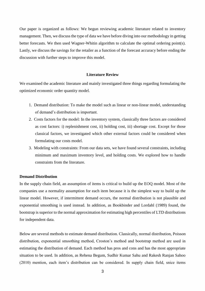
Figure 1 shows the actual outbound demand versus the retailer’s currently demand forecast. This

figure demonstrates the major cause of their high inventory costs they were facing.

8

Figure 1: Actual Demand vs Demand Forecast

We began observing large differences between the retailer’s forecast and the actual demand, which

translated into high inventory management costs in form of underage costs and holding costs. Further

we see different patterns in demand that led us to cluster the items into different clusters to deal with

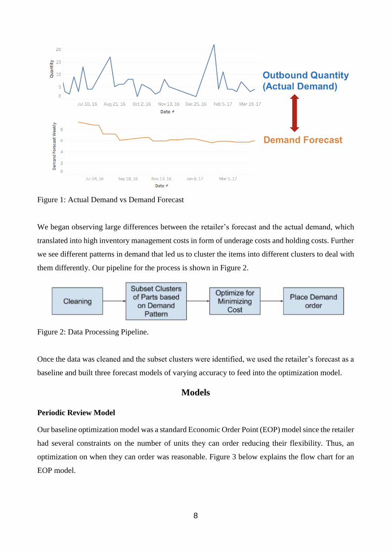
them differently. Our pipeline for the process is shown in Figure 2.

Figure 2: Data Processing Pipeline.

Once the data was cleaned and the subset clusters were identified, we used the retailer’s forecast as a

baseline and built three forecast models of varying accuracy to feed into the optimization model.

Models

Periodic Review Model

Our baseline optimization model was a standard Economic Order Point (EOP) model since the retailer

had several constraints on the number of units they can order reducing their flexibility. Thus, an

optimization on when they can order was reasonable. Figure 3 below explains the flow chart for an

EOP model.

9

Figure 3: Economic Order Point

Following the above flowchart, EOP is a continuous review process where we check if we reached a

pre-determined re-order point after every order fulfillment and we trigger an order if we did reach a

re-order point.

Exponential Smoothing with Trend

Exponential Smoothing refers to an averaging method that weighs the most recent data more strongly.

This is useful if the data changes as a result of seasonality (or pattern) instead of a random walk.

Mathematically, this can be written as

𝐹𝑡+1 = ∝ 𝐷𝑡 + (1−∝)𝐹𝑡

where Ft+1 = Forecast for the next time period

Dt = Actual Demand at time t

Ft = Forecast at time t

= Weighing factor referred to as a smoothing parameter

This can be enhanced by adding a trend adjustment factor to incorporate the trend into the equation.

𝐴𝐹𝑡+1 = 𝐹𝑡+1 + 𝑇𝑡+1𝑎𝑛𝑑

𝑇𝑡+1 = 𝛽(𝐹𝑡+1 − 𝐹𝑡) + (1 − 𝛽)𝑇𝑡

where At = Adjusted Forecast for time t+1

Tt = Last period’s trend factor and

= Smoothing parameter for trend

10

For this model, people tend to use Mean Average Deviation (MAD) as the metric of determination.

Dynamic Programming

We used the Wagner-Whitin algorithm to help decide the time of the re-order point. The Wagner-

Whitin Algorithm divides the n-period optimization problem to a series of sub-problems and each

sub-problem is solved and used in solving the next sub problem. For example, if the decision maker

wishes to plan his reorder point for six periods, the model divides his 6-period problem into six single

period problems. On week 1, the decision maker has six options, order for all six weeks, order for the

first five weeks, etc. all the way down to just ordering for just the first week. Choosing the option that

minimizes the sum of holding cost and ordering cost would be the best decision for the decision

maker. The series of such recurrent decisions made for all six periods gives us the overall minimum

cost path. Mathematically,

Step 1: t = 1, zt* = 0 Step 2: t = t+1. If t > T+1, stop. Otherwise go to step 3. Step 3: For all t’ = 1, 2, …, t - 1,

', ' ' ' 1 ' ' 1 1

' 1 ' 2 1 2 1

( ... ) ( ... )

( ... ) ...

t t t t t t t t t

t t t t t

c A c D D h D D

h D D h D

- + -

+ + - - -

= + + + + + + +

+ + + +

Step 4: Compute

}{min ,'*'

1,...,2,1'

*ttt

ttt czz +=

-=

Step 5: Compute

* *' ',

' 1,2,..., 1

arg min{ }t t t tt t

p z c= -

= +

that is, choose the period t’ that minimizes ttt cz ,'*' +

Step 6: Go to step 2.

The optimal cost is given by *

1Tz + The optimal set of periods in which ordering/production takes place can be obtained by

backtracking from *

1Tp +

11

Results

Based on the above model, we calculated the total cost of inventory management for different

products and it is observed that we are able to save about 13.7 % using the actual demand +/- a random

value of 1 unit (which gives us an accuracy rate of 85%). We can save up to 20% in inventory costs

using the dynamic model developed.

We also added an additional parameter into the equation that penalized the retailer for understocking.

For example, there was only opportunity cost previously, but we considered the possibility of

backordering which would inflict 1.5 times the cost for the retailer, and this caused an additional

saving of 20% because of the optimization.

Conclusion

As discussed, forecasting and optimization go hand in hand when it comes to inventory optimization.

Accurate forecasts lead to lower costs. Figure 4 shows the relationship we found when comparing the

demand forecasting model’s accuracy and the decisions the inventory decisions that would occur

because of the model.

Figure 4: Model accuracy versus total costs ($)

In summary, we compared the results from our model for the three predicted demands to see which

one performed better based on the accuracy of demand. We used total cost incurred during the period

under consideration including the cost of stock-outs as a metric to compare the performance. We

found that the client’s predicted demand had the highest total cost associated with it due to poor

accuracy. Our attempt to use the Exponential Smoothing technique to simulate predicted demand did

not yield an accurate forecast. As the model with highly accurate predicted demand showed least total

12

cost, we suggest the client to improve their accuracy of demand forecast, and thus realize better

inventory performance.

References

Kun-Jen Chung, Leopoldo Eduardo Cárdenas-Barrón (2012). “The complete solution procedure for

the EOQ and EPQ inventory models with linear and fixed backorder costs” Mathematical and

Computer Modelling 55 (2012): 2151–2156.

Mark Ferguson, Vaidy Jayaraman, Gilvan C. Souza “An Application of the EOQ Model with

Nonlinear Holding Cost to Inventory Management of Perishables”.

Elsayed, E. A., and C. Teresi (1983). “Analysis of Inventory Systems with Deteriorating Items.”

International Journal of Production Research, 21(4): 449-460.

Weiss, H. (1982). “Economic Order Quantity Models with Nonlinear Holding Costs.” European

Journal of Operational Research 9:56–60.

Sridhar Bashyam, Michael C. Fu (1997). “Optimization of Inventory Systems with Random Lead

Times and a Service Level Constraints” Management Science.

Ilkyeong Moon, Sangjin Choi (1994). “The Distribution Free Continuous Review Inventory System

with a Service Level Constraint” Computers ind. Engng Vol. 27, Nos 1-4, pp. 209-212.

James H. Bookbinder, Jin Yan Tan (1988) “Strategies for the Probabilistic Lot-Sizing Problem with

Service-Level Constraints” Management Science, September.

L.A. San-José, n, J. Sicilia, J. García-Laguna (2015) “Analysis of an EOQ inventory model with

partial backordering and non-linear unit holding cost” Omega 54 (2015) 147–157.

Wen-Yang Lo*, Chih-Hung Tsai, Rong-Kwei Li (2002) “Exact solution of inventory replenishment

policy for a linear trend in demand - two-equation model” Int. J. Production Economics 76(2002)

111-120

13

B. N. Mandal, S. Phaujdar (1989) “An Inventory Model for Deteriorating Items and Stock-dependent

Consumption Rate” J. Opt Res Soc Vol.40 No.5 pp 483, 488

Rehena Begum, Sudhir Kumar Sahu, Rakesh Ranjan Sahoo (2010) “An EOQ model for deteriorating

items with Weibull distribution deterioration, unit production cost with…”.

ARIS A. SYNTETOS, JOHN E. BOYLAN (2008) “Demand forecasting adjustments for service-

level achievement” IMA Journal of Management Mathematics (2008) 19, 175−192.

Chris Dubelaar, Garland Chow, Paul D. Larson (2001) “Relationships between inventory, sales

and service in a retail chain store operation”

Thomas R. Willemain*, Charles N. Smart, Henry F. Schwarz (2004) “A new approach to forecasting

intermittent demand for service parts inventories” International Journal of Forecasting 20 (2004) 375–

387.

G. Padmanabhan a, Prem Vrat (1989) “EOQ models for perishable items under stock dependent

selling rate”

Banker, Steve (2013). “Demand Forecasting: Going Beyond Historical Shipment Data.” Retrieved

from : https://www.forbes.com/sites/stevebanker/2013/09/16/demand-forecasting-going-beyond-

historical-shipment-data/#70623c2c16fb

Banker, Steve (2013). “Demand Forecasting: Going Beyond Historical Shipment Data.” Retrieved

from: https://www.forbes.com/sites/stevebanker/2013/09/16/demand-forecasting-going-beyond-

historical-shipment-data/#70623c2c16fb

Rosenblum, Paula (2014). “Walmart's Out of Stock Problem: Only Half the Story?” Retrieved from:

https://www.forbes.com/sites/paularosenblum/2014/04/15/walmarts-out-of-stock-problem-only-

half-the-story/

Banker, Steve (2015). “Transportation and Inventory Optimization are Becoming More Tightly

Integrated.” Retrieved from: https://www.forbes.com/sites/stevebanker/2015/08/10/transportation-

and-inventory-optimization-are-becoming-more-tightly-integrated/#4a311d0c608f

14

Marr, Bernard (2016). “How Big Data and Analytics Are Transforming Supply Chain Management.”

Retrieved from: https://www.forbes.com/sites/bernardmarr/2016/04/22/how-big-data-and-analytics-

are-transforming-supply-chain-management/#5b63c62439ad

Fritsch, Daniel (2017). “Purchase Planning: Basics, Considerations, & Best Practices.” Retrieved

from: https://www.eazystock.com/blog/2017/03/09/purchase-planning-basics-considerations-best-

practices/