Embed Size (px)
Citation preview
Effect of Farm Income Risk on Smallholder Production Decisions
in the Highlands of Machakos District, Kenya:
The Case of Kauti Irrigation Scheme
By
Elijah N. No: A512/70462/2007)
A thesis submitted to the Department of Agricultural Economics, University of
Nairobi, in partial fulfillment of the requirements for the degree of
Master of Science in Agricultural and Applied Economics
University of NAIROBI Library
September, 2010
UNIVERSITY OF NAIHH8IKAEEl k LIBRARY

1
Declaration
I, Elijah Nzula Muange, declare that this thesis is my original work and
has not been presented for a degree award in any university.
Signature Date
Elijah N. Muange
(Reg. No: A512/70462/2007)
This thesis has been submitted for examination with our approval as
Professor Chris Ackello-Ogutu
Signature .....Date . | b j ^ j f
Dr. S. M. Mukoya-Wangia
11
Acknowledgements
This work would not have been possible without the contributions of the following persons.
First are my supervisors Prof. C. Ackello-Ogutu and Dr. S. Mukoya-Wangia who tirelessly
helped me to nurture the thesis concept and develop it into a full thesis. Second is Dr. R.A.
Nyikal, whose input and inspiration were very instrumental in motivating me. Third is the
Ministry of Agriculture extension staff at the Machakos District and Kathiani Divisional
agricultural offices for their generous information and support during my fieldwork.
Fourthly, the staff at the Department of Agricultural Economics and Kabete Library
facilitated access to literature for the preparation of this thesis. Your kindness is greatly
appreciated. Finally are all members of the academic staff and fellow students in the
Department of Agricultural Economics for their criticism, advice and encouragement. To all
I say a big thank you.

Ill
Dedication
To my wife; Judy, and Children; Esther and David, for your love, support, inspiration and
encouragement during my study period.
To my Mother Esther, and Late dad Muange, who introduced me to the academic world.
IV
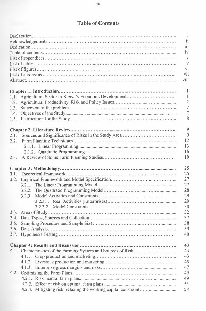
Table of Contents
Declaration........................................................................................................................ iAcknowledgements........................................................................................................... iiDedication......................................................................................................................... iiiTable of contents............................................................................................................... ivList of appendices............................................................................................................. vList of tables...................................................................................................................... vList of figures.................................................................................................................... viList of acronyms............. viiAbstract............................................................................................................................. viii
Chapter 1: Introduction................................................................................................. 11.1. Agricultural Sector in Kenya’s Economic Development........................................ 11.2. Agricultural Productivity, Risk and Policy Issues................................................... 21.3. Statement of the problem......................................................................................... 71.4. Objectives of the Study............................................................................................ 71.5. Justification for the Study........................................................................................ 8
Chapter 2: Literature Review....................................................................................... 92.1. Sources and Significance of Risks in the Study Area........................................... 92.2. Farm Planning Techniques..................................................................................... 12
2.1.1. Linear Programming................................................................................. 132.1.2. Quadratic Programming............................................................................ 16
2.3. A Review of Some Farm Planning Studies.......................................................... 19
Chapter 3: Methodology................................................................................................ 253.1. Theoretical Framework............................................................................................ 253.2. Empirical Framework and Model Specification...................................................... 27
3.2.1. The Linear Programming Model................................................................. 273.2.2. The Quadratic Programming Model............................................................ 283.2.3. Model Activities and Constraints................................................................. 29
3.2.3.1. Real Activities (Enterprises)......................................................... 293.2.3.2. Model Constraints......................................................................... 30
3.3. Area of Study........................................................................................................... 323.4. Data Types, Sources and Collection........................................................................ 373.5. Sampling Procedure and Sample Size..................................................................... 383.6. Data Analysis........................................................................................................... 393.7. Hypothesis Testing................................................................................................ 40
Chapter 4: Results and Discussion................................................................................ 434.1. Characteristics of the Farming System and Sources of Risk................................... 43
4.1.1. Crop production and marketing................................................................... 434.1.2. Livestock production and marketing............................................................ 454.1.3. Enterprise gross margins and risks.............................................................. 47
4.2. Optimizing the Farm Plans...................................................................................... 494.2.1. Risk-neutral farm plans................................................................................ 494.2.2. Effect of risk on optimal farm plans............................................................ 534.2.3. Mitigating risk: relaxing the working capital constraint.............................. 58
V
Chapter 5: Summary, Conclusions and Recommendations........................................ 645.1. Summary and Conclusions.......................................................................................5.2. Recommendations for Policy and Further Research................................................ 64
67References....................................................................................................................... 71
List of AppendicesAppendix 1: Focus Group Discussion Schedule.............................................................. 77Appendix 2: Household Survey Questionnaire................................................................ 79Appendix 3: Gross Margin Calculations for Livestock Enterprise................................... 87Appendix 4: Risk-neutral (Linear Programming) model input data................................. 88Appendix 5: Risk-neutral (Quadratic Programming) model input data.................. 89Appendix 6: Alternative farm plans for subsistence model under constrained
capital........................................................................................................ 90Appendix 7: Alternative farm plans for non-subsistence model under constrained
capital........................................................................................................ 90Appendix 8: Alternative farm plans for subsistence model under relaxed capital in
season 1..................................................................................................... 91Appendix 9: Alternative farm plans for subsistence model under relaxed capital in
season 2..................................................................................................... 91Appendix 10: Alternative farm plans for subsistence model under relaxed capital in
season 1&2............................................................................................... 92
List of TablesTable 1.2: Gross Margins of Selected Crops under Rainfed and Irrigation Farming in Kenya.... 27Table 3.2(a): Man equivalents of persons of different age categories.............................. 31Table 3.2(b): List of constraints used in the mathematical programming models............ 33Table 3.3.2: Administrative units and population data of Kathiani Division................... 34Table 3.5: Population and sample size per village............................................................ 39Table 4.1.1(a): Adoption of certified seed, manure and fertilizer in key crops................ 43Table 4.1.1(b): Key input prices faced by farmers in 2007-08 short rains season........... 44Table 4.1.1(c): Observed and potential yields of the main crops..................................... 44Table 4.1.1(d): Output prices of major crops (2007-08).................................................. 45Table 4.1.2(a): Main livestock kept, their production systems and stocking rate............ 46Table 4.1.2(b): Livestock unit equivalents of different categories of livestock............... 46Table 4.1.2(c): Main livestock products and their utilization.......................................... 47Table 4.1.3(a): Gross margins of key enterprises............................................................ 47Table 4.1.3(b): Variance-covariance matrix for enterprise gross margins...................... 48Table 4.2.1(a): Comparison between current and risk-neutral optimal farm plans.............. 50Table 4.2.1(b): t-test results for equality of existing and optimal TFGM....................... 51Table 4.2.1(c): Optimal resource allocation and marginal values................................... 52Table 4.2.2(a): Risk-efficient farm plans for the subsistence model............................... 53Table 4.2.2(b): Risk-efficient farm plans for the non-subsistence model........................ 56Table 4.2.3(a): Risk-efficient farm plans for a subsistence model with unconstrained
capital in season 1............................................................................... 60Table 4.2.3(b): Risk-efficient farm plans for a subsistence model with unconstrained
capital in season 2............................................................................... 61Table 4.2.3(c): Risk-efficient farm plans for a subsistence model with unconstrained
capital in seasons 1&2......................................................................... 62Table 5.2: Recommended risk-efficient farm plans........................................................... 67

VI
List of FiguresFigure 2.1(a): 10-year rainfall data for Katumani research station, Machakos............... 10Figure 2.1(b): Quarterly fertilizer prices in Kathiani Market (July 2007- March
2008)......................................................................................................... 11Figure 2.1(c): Quarterly farm gate prices of selected crops in Kathiani (Oct 2007- Dec
2008)......................................................................................................... 11Figure 3.1: Process of choosing a risk-efficient enterprise mix by a farmer.................... 27Figure 3.3.1: A Map of Machakos District Showing Kathiani Division.......................... 35Figure 3.3.2: A Map of Kathiani Division Showing Kauti Irrigation Scheme................. 36Figure 4.2.2(a): EV Frontier for the Subsistence Model................................................... 55Figure 4.2.2(b): EV Frontier for the Non-subsistence Model........................................... 57Figure 4.2.3: Risk-efficient EV frontier map for constrained and unconstrained seasonal
capital in a farm model with subsistence constraints................................. 63
Vll
EV
List of Acronyms
Mean-Variance combination of income associated with a farm plan
GAMS General Algebraic Modelling System
Ksh Kenya Shilling(s)
LP Linear Programming
LU Livestock Unit(s)
MVP Marginal Value Product
QRP Quadratic Risk Programming
SPSS Statistical Package for Social Sciences
TFGM Total Farm Gross Margin
Vlll
Abstract
Raising agricultural productivity and incomes in the densely populated highlands of
Machakos District is constrained by various risks which make farm income uncertain.
Farmers diversify their activities to cushion themselves against risks but there is no empirical
recommendation to guide them in selecting optimal enterprise combinations (farm plans).
The farmers adopt own-preferred farm plans but it is not known whether such plans
minimize risk. This study assessed the effect of farm income risks on production decisions in
Kauti Irrigation Scheme, with a view to identifying farm plans that earn farmers higher
incomes at existing or lower levels of income risk.
The study used crop and livestock production and marketing data covering 2007/08 and
2008 rain seasons, collected in March 2009 through a farm household survey involving 113
households. The data were analysed using linear and quadratic risk programming techniques.
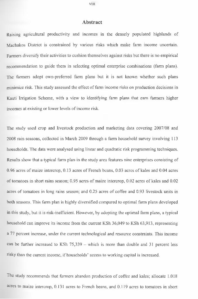
Results show that a typical farm plan in the study area features nine enterprises consisting of
0.96 acres of maize intercrop, 0.13 acres of French beans, 0.03 acres of kales and 0.04 acres
of tomatoes in short rains season; 0.95 acres of maize intercrop, 0.02 acres of kales and 0.02
acres of tomatoes in long rains season; and 0.25 acres of coffee and 0.93 livestock units in
both seasons. This farm plan is highly diversified compared to optimal farm plans developed
in this study, but it is risk-inefficient. However, by adopting the optimal farm plans, a typical
household can improve its income from the current KSh 36,049 to KSh 63,913, representing
a 77 percent increase, under the current technological and resource constraints. This income
can be further increased to KSh 75,339 - which is more than double and 31 percent less
risky than the current income, if households’ access to working capital is increased.
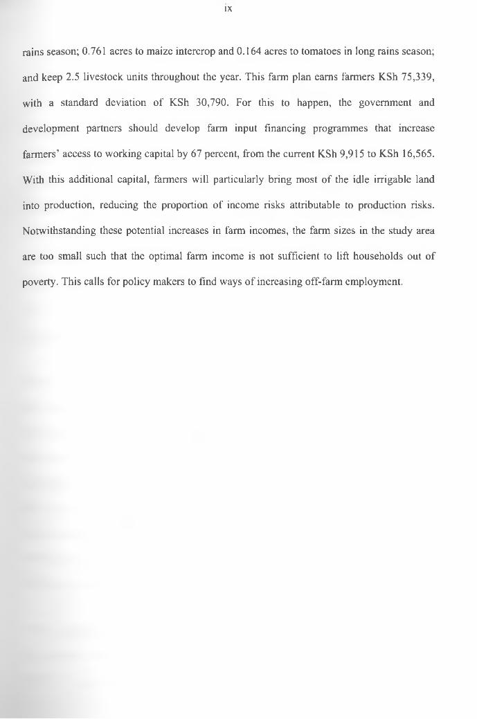
The study recommends that farmers abandon production of coffee and kales; allocate 1.018
acres to maize intercrop, 0.131 acres to French beans, and 0.119 acres to tomatoes in short
IX
rains season; 0.761 acres to maize intercrop and 0.164 acres to tomatoes in long rains season;
and keep 2.5 livestock units throughout the year. This farm plan earns farmers KSh 75,339,
with a standard deviation of KSh 30,790. For this to happen, the government and
development partners should develop farm input financing programmes that increase
farmers’ access to working capital by 67 percent, from the current KSh 9,915 to KSh 16,565.
With this additional capital, farmers will particularly bring most of the idle irrigable land
into production, reducing the proportion of income risks attributable to production risks.
Notwithstanding these potential increases in farm incomes, the farm sizes in the study area
are too small such that the optimal farm income is not sufficient to lift households out of
poverty. This calls for policy makers to find ways of increasing off-farm employment.
Chapter 1: Introduction
1.1. Agricultural Sector in Kenya’s Economic Development
Reduction of poverty and unemployment remain the two major development challenges
facing Kenya. The government plans to reduce the proportion of its population living below
the poverty line from 56 percent in 2000 to 26 percent by 2015, and the proportion of the
food poor from 48.4 percent to below 10 percent by the year 2015, in line with the United
Nations Millennium Development Goal number one (Republic of Kenya, 2004a). To achieve
these objectives, the agricultural sector will play a pivotal role, particularly because the
sector contributes about 22 percent of the country’s gross domestic product (GDP), and is
also the main source of livelihood for approximately 80 percent of the country’s rural
population (Republic of Kenya, 2008 and Kenya National Bureau of Statistics, 2009).
Kenya’s agriculture sector is faced with a myriad of challenges including frequent droughts
and floods, lack of farmer’s access to credit, low adoption of modem technology, poor
governance and corruption in major agricultural institutions, inadequate markets and market
infrastructure and high costs of inputs, which slow down the performance of the sector
(Republic of Kenya, 2004b). For the sector to perform its role in improving incomes and
food security, efforts should therefore be geared towards raising productivity,
commercializing agriculture, improving input and produce markets, encouraging
diversification into high value enterprises and strengthening and reforming agricultural
institutions (Eicher and Staatz, 1998, Fan and Chan-Kang, 2005 and World Bank, 2008).
Raising agricultural productivity is important in an agriculture-based country such as Kenya
for a number of reasons. First, agriculture is the main food producing sector and therefore,
increase in food productivity will improve food security in the country (Kinyua, 2004).
- 1 -
- 2 -
Secondly, the sector accounts for 80 percent of employment as mentioned above, 60 percent
of export earnings and 45 percent of government revenue (Sikei et al, 2009), and these are
likely to improve with increased productivity. Thirdly, agricultural productivity (particularly
of staples) affects food prices and consequently wage costs and competitiveness of tradable
sectors (World Bank, 2008). Kenya’s economy depends on agriculture for its tradable
sectors, which are basically primary industries such as agro-processing. Agricultural
productivity is therefore crucial in determining the price of raw materials used in the tradable
sectors and hence their competitiveness. This makes a case for improving agricultural
productivity in the country.
1.2. Agricultural Productivity, Risk and Policy Issues
Agricultural output and productivity in Kenya is low in dry lowland regions such as
Machakos, compared to the high rainfall areas (Kibaara et al, 2009). Key drivers of
productivity in the country are well documented and they include high yielding varieties and
animal breeds, use of inorganic fertilizers, access to rural financial services and reduced
distances to agricultural extension services, input stockists and motorable roads (Kibaara et
al, 2009). In the SRA (Republic of Kenya 2004b), the government outlines a number of
measures that will ensure improvement of the above factors, but recent studies (Ariga et al,
2008 and Kibaara et al, 2009) show many of these factors are still unfavourable in the
dryland areas.
One way of raising agricultural productivity in Kenya even under the existing technological,
resource and institutional constraints is through proper planning of farm activities in order to
enhance efficiency in utilization of the scarce productive resources. However, the farming
environment, especially in the arid areas, is very risky and the risk aversive behaviour of
farmers constrains adoption of optimal farm plans, leading to misallocation of resources
(Hardaker et al, 2004 and Msusa, 2007). Past studies (Owuor, 1999; Freeman and Omiti,
2003 and Kibaara et al 2009) show that adoption of productivity improving inputs and
technologies is very low mainly due to risky farming environment occasioned by low and
erratic rainfall. Thus, given that risks affect farm decisions, the extent to which risks and
their effect on farmers’ decision-making are understood can determine success of programs
aimed at raising agricultural productivity and incomes, and consequently rural development
(Olarinde, et al, 2008).
The distinction between risk and uncertainty was at first made by Frank Knight (quoted in
Debertin, 2002). Knight postulated that in a risky environment, both event outcomes and
their probabilities of occurrence are known; whereas in an uncertain environment, neither the
outcomes nor their respective probabilities of occurrence are known. But Debertin (2002)
puts a very thin divide between risk and uncertainty. He sees a risk-uncertainty continuum,
with purely risky events on one extreme and purely uncertain events on the other extreme. In
between the two extremes is an environment in which only some possible outcomes are
known and only some outcomes have probabilities attached to them. It is in this mid-point
that most farmers operate.
In Kenyan agriculture, risks are of several forms, as highlighted by (Kliebenstein and Scott
JR., 1975, Hardaker et al, 2004, and Bhowmick, 2005).These include production risks,
caused by extremities of weather elements like rainfall, humidity and temperature and
biological organisms such as pests and diseases; market risks, caused by fluctuations in input
and output prices, currency exchange rates and product demand; and institutional risks,
emanating from unfavourable changes in government policies such as increases in taxes. If
unabated, the above types of risk translate into farm income risks and consequently low
agricultural productivity (Kuyiah et al, 2006).
-3 -
- 4 -
Smallholder farmers are not unaware of risks and in their bid to cope with them; they adopt
several mechanisms such as enterprise diversification, mixed cropping and irrigation
(Kliebenstein and Scott JR., 1975, Rafsnider, et al, 1993, Bhowmick, 2005 and Umoh,
2008). Irrigation has the potential to reduce farming risks associated with stochastic rainfall,
thereby increasing farm productivity, output and consequently incomes (FAO, 2003). In
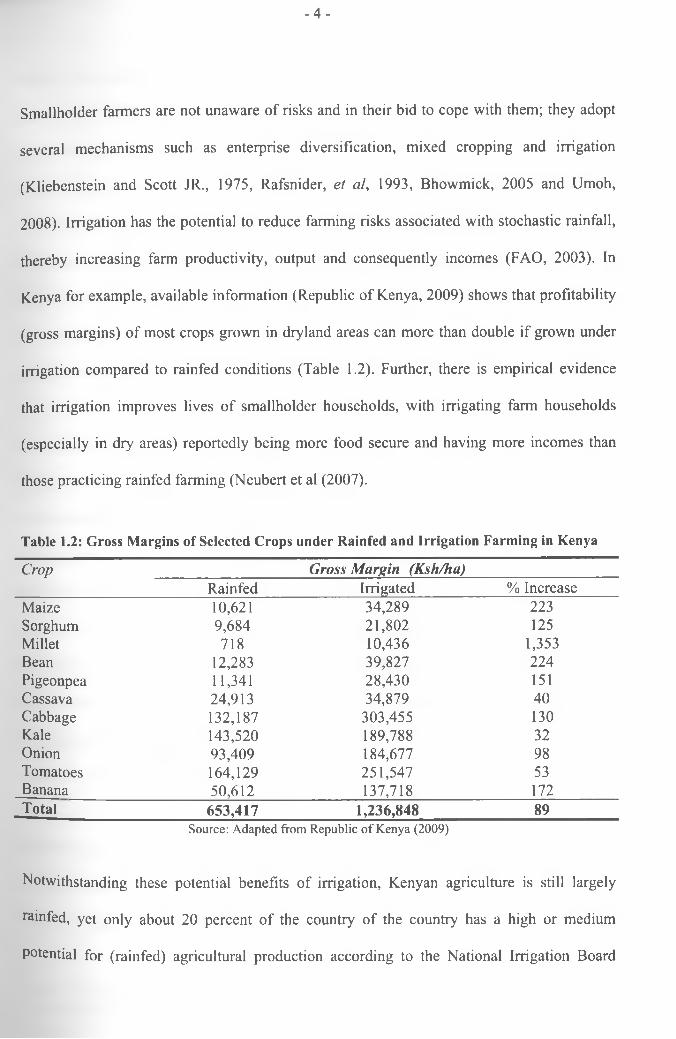
Kenya for example, available information (Republic of Kenya, 2009) shows that profitability
(gross margins) of most crops grown in dryland areas can more than double if grown under
irrigation compared to rainfed conditions (Table 1.2). Further, there is empirical evidence
that irrigation improves lives of smallholder households, with irrigating farm households
(especially in dry areas) reportedly being more food secure and having more incomes than
those practicing rainfed farming (Neubert et al (2007).
Table 1.2: Gross Margins of Selected Crops under Rainfed and Irrigation Farming in Kenya
Crop Gross Margin (Ksh/ha)Rainfed Irrigated % Increase
Maize 10,621 34,289 223Sorghum 9,684 21,802 125Millet 718 10,436 1,353Bean 12,283 39,827 224Pigeonpea 11,341 28,430 151Cassava 24,913 34,879 40Cabbage 132,187 303,455 130Kale 143,520 189,788 32Onion 93,409 184,677 98Tomatoes 164,129 251,547 53Banana 50,612 137,718 172Total 653,417 1,236,848 89
Source: Adapted from Republic o f Kenya (2009)
Notwithstanding these potential benefits of irrigation, Kenyan agriculture is still largely
rainfed, yet only about 20 percent of the country of the country has a high or medium
potential for (rainfed) agricultural production according to the National Irrigation Board
- 5 -
(NIB)1. Out of the total potential irrigable land of 497,400 hectares, only about 183,900
hectares (37 percent) had been developed as at 2007, but the government plans to expand
irrigated land to 300,000 hectares by 2012 in line with its Vision 2030 goals (Republic of
Kenya, 2009). However, irrigation development in Kenya faces numerous challenges
including lack of a national irrigation policy, legal and institutional frameworks; inadequate
investment in the sector by both public and private sector; inadequate development of
irrigation infrastructure and water storage facilities; inadequate technical capacity for both
the technical staff and farmers; inadequate farmers’ organization and participation and
inadequate support services such as credit, infrastructure and extension (Mbatia, 2006).
Machakos District has an irrigation potential of 10,000 hectares, but only about one third of
this potential (3,000 hectares) is irrigated . Most of the irrigation is practiced under small
scale community irrigation schemes/projects managed by water user associations/groups.
The projects source water from rivers, springs and dams and vary in size from about 2 to 800
hectares. Farmers in these schemes grow horticultural crops mainly for the market, but some
also use irrigation water to supplement inadequate rainfall in subsistence crops. The main
challenges experienced in the irrigation schemes are inadequate water, soil erosion problems
due to steep slopes, high water losses due to seepage and evaporation during conveyance,
crop pests and diseases that reduce quality and quantity of marketable produce, and poor
marketing arrangements for farm produce.
In Kathiani, the study Division, there are ten small scale farmer-managed irrigation schemes,
of which Kauti is the largest. Kauti Irrigation Scheme uses a gravity fed open furrow
irrigation system. Irrigation water is sourced from Umanthi River and Muooni dam, built 2
2 http.//www.nib.or.ke. Accessed on 30th August 2010ccording to various unpublished reports at the District Agricultural Office, Machakos.
- 6 -
along the same river, and is conveyed through four unlined canals. The estimated number of
farmers in the scheme is 1,000. Although the initial purpose of the scheme was to introduce
commercial farming, not all farmers practice irrigation in all seasons. The number of farmers
irrigating during each season fluctuates depending on water availability and socioeconomic
factors (Ministry of Agriculture 2005). Farmers are not formally restricted on the size of land
or crops to irrigate. The choice of these depends on how well the farmer can manage the
irrigation water allocated to him/her. The main irrigated crops grown are kales, tomatoes and
French beans, while maize, beans, pigeon peas, cowpeas, coffee, bananas, mangoes and
avocadoes are mainly rain-fed though some farmers irrigate to supplement rainfall when it is
insufficient. The farmers also keep cattle, goats, sheep and chicken.
Several problems experienced in the scheme limit profitability of farming in the area. These
include: reduced dam capacity due to siltation; canal degradation, which has reduced canal
length from the initial 10 kilometres to less than 5 kilometres at present; high water losses
through seepage and evaporation during conveyance; weak management system, with some
farmers refusing to participate in management of the canals; lack of working capital; and
poor marketing arrangements. These challenges expose farmers to many risks particularly
due to the erratic nature of rainfall, irrigation water supply, and input and output prices. The
scheme is currently being rehabilitated with funding from African Development Bank
(ADB) to address most of these problems. But while these rehabilitation efforts go on,
farmers face a key challenge of determining the type, number and level of enterprises that
they must operate in their small farms in order to use the available irrigable land and other
resources more efficiently and maximise their incomes while minimising risks3.
Additional information from a focus group discussion with farmers and discussions with Ministry of Agriculture extension staff in Kathiani Division.
1.3. Statement of the Problem
Farmers in Kauti Irrigation Scheme are faced with numerous risks, which make farm
incomes uncertain. In an attempt to cushion themselves against this income risk, the farmers
resort to diversification of farm enteiprises. However, no study has been carried out in the
Scheme to determine optimal enterprise mixes (farm plans) that suits each farmer’s degree of
risk aversion. This is complicated by the small farm sizes which limit the degree of
diversification, yet the fanners desire to operate as many enterprises as possible. In the
absence of formally recommended optimal farm plans, farmers adopt own-preferred
enterprise mixes, which reportedly misallocate resources and reduce farm incomes, as the
farmers trade off expected income with risk (Bhende and Venkataram, 1994 and Kobzar,
2006). The low income levels in the Scheme call for improvement of the farming system in
order to raise farm incomes and reduce income risks.
1.4. Objectives of the Study
The general objective of the study was to assess the effect of farm income risks on
production decisions, with a view to identifying farm plans that earn farmers higher incomes
at existing or lower levels of risk. Specific objectives were to:
i. determine optimal farm plans and compare them with the existing plans
ii. assess the effect of farm income risk on choice of optimal farm plans
iii. investigate risk mitigating strategies that would enable farmers increase incomes at
the existing or lower levels of income risk.
The hypotheses tested were that existing farm plans are optimal; and secondly, that risk
preference does not affect choice of optimal farm plans in the study area.
- 7 -
- 8 -
1.5. Justification for the Study
Food security and poverty are major development challenges in Machakos District. Although
about 70 percent of the population derive their livelihood from agriculture, low output and
productivity and high farming risks threaten improvement of food security and farm
incomes. With limited and decreasing per capita land, particularly in the densely populated
highlands of the district, growth in agricultural output can hardly come from cultivating
additional land, but rather from growth in productivity (Kibaara, et al, 2009). This
productivity growth will result from improved efficiency in production as envisaged in the
current Strategy for Revitalizing Agriculture (Republic of Kenya, 2004b) and by Adesiyan et
al, (2007). One way of improving production efficiency in Machakos is by adoption farm
plans that optimize risk, and this study contributes to the existing literature on how such
plans can be generated.
- 9 -
Chapter 2: Literature Review
This chapter begins with a discussion on some of the main sources of farm income risks in
the study area. It then introduces approaches to farm planning and enumerates some of the
main risk programming techniques used in farm planning. The two farm planning techniques
adopted in the study (linear programming and quadratic risk programming) are also
discussed and in the final part of the chapter, summaries of some farm planning studies that
have applied linear and quadratic programming techniques within and outside the country
are reviewed.
2.1 Sources and Significance of Farming Risks in the Study Area
Among the main risks that affect agricultural production and incomes in Machakos District
are erratic rainfall and input and output prices. The erratic nature of these factors has been
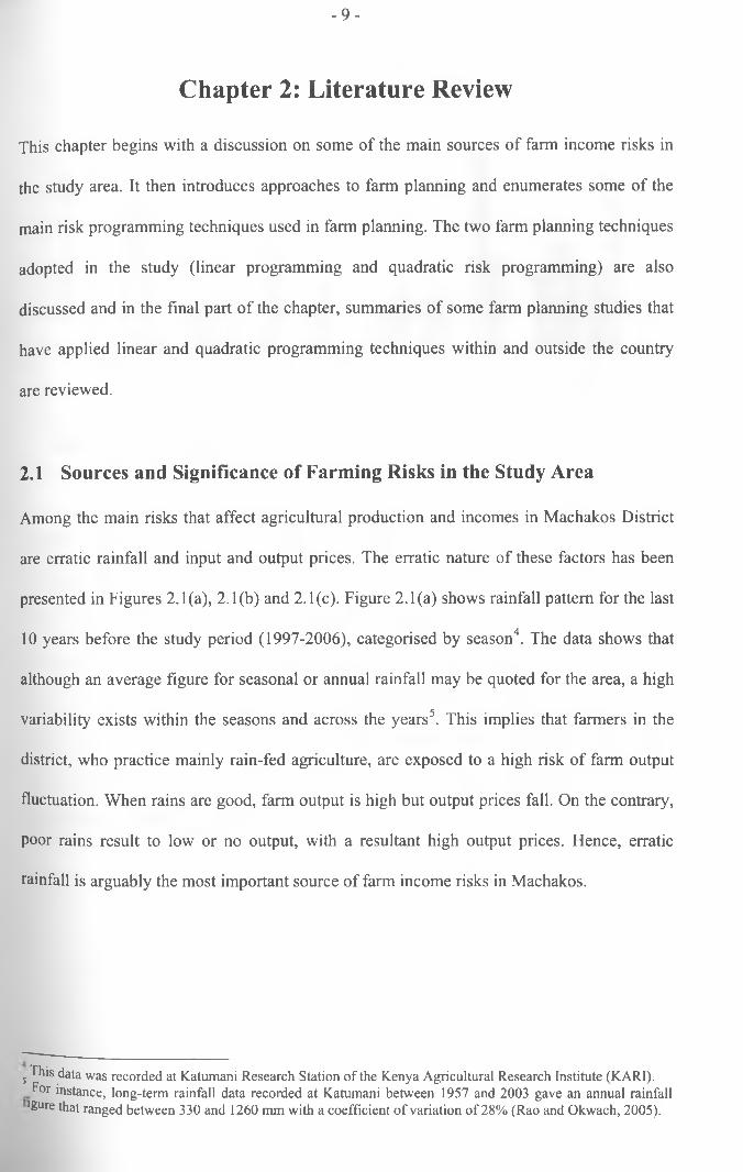
presented in Figures 2.1(a), 2.1(b) and 2.1(c). Figure 2.1(a) shows rainfall pattern for the last
10 years before the study period (1997-2006), categorised by season4. The data shows that
although an average figure for seasonal or annual rainfall may be quoted for the area, a high
variability exists within the seasons and across the years5. This implies that farmers in the
district, who practice mainly rain-fed agriculture, are exposed to a high risk of farm output
fluctuation. When rains are good, farm output is high but output prices fall. On the contrary,
poor rains result to low or no output, with a resultant high output prices. Flence, erratic
rainfall is arguably the most important source of farm income risks in Machakos.
s This data was recorded at Katumani Research Station o f the Kenya Agricultural Research Institute (KARI).For instance, long-term rainfall data recorded at Katumani between 1957 and 2003 gave an annual rainfall
■gore that ranged between 330 and 1260 mm with a coefficient o f variation of 28% (Rao and Okwach, 2005).
- 10 -
Figure 2.1(a): 10-year rainfall data for Katumani research station, Machakos
Data Source: District Agricultural Office, Machakos (2009)
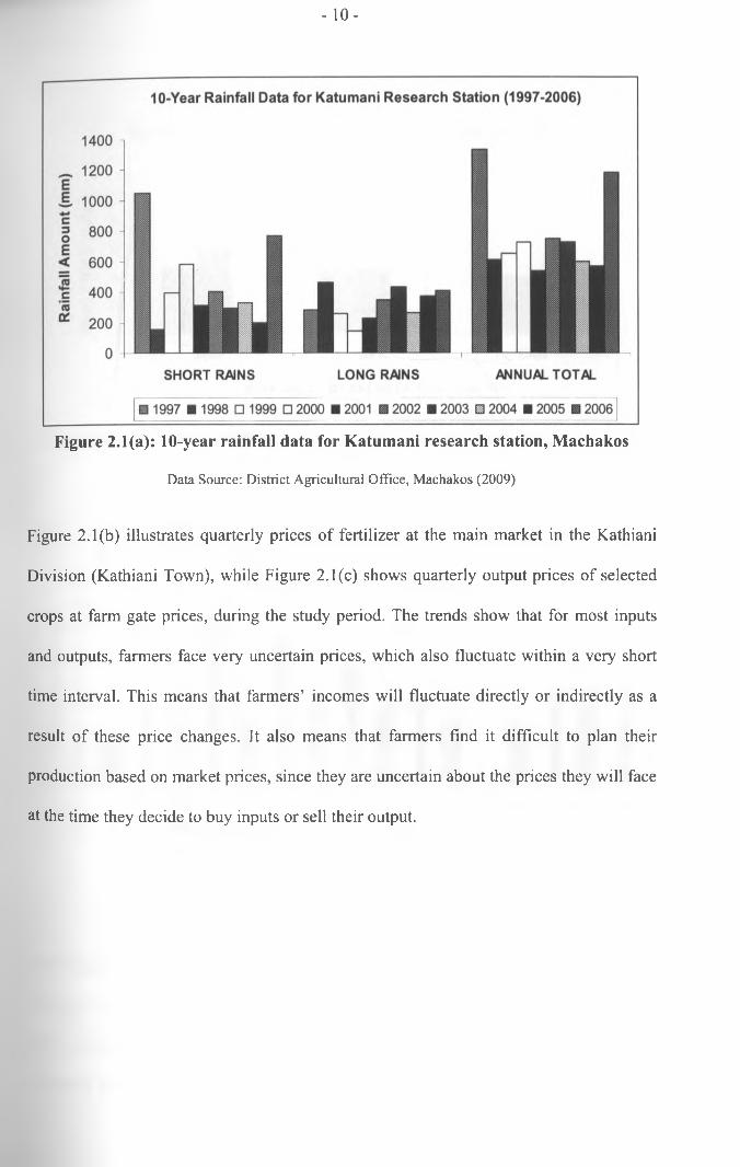
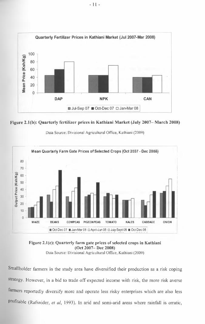
Figure 2.1(b) illustrates quarterly prices of fertilizer at the main market in the Kathiani
Division (Kathiani Town), while Figure 2.1(c) shows quarterly output prices of selected
crops at farm gate prices, during the study period. The trends show that for most inputs
and outputs, farmers face very uncertain prices, which also fluctuate within a very short
time interval. This means that farmers’ incomes will fluctuate directly or indirectly as a
result of these price changes. It also means that farmers find it difficult to plan their
production based on market prices, since they are uncertain about the prices they will face
at the time they decide to buy inputs or sell their output.
- 1 1 -
Figure 2.1(b): Quarterly fertilizer prices in Kathiani Market (July 2007- March 2008)
Data Source: Divisional Agricultural Office, Kathiani (2009)
Mean Quarterly Farm Gate Prices of Selected Crops (Oct 2007 - Dec 2008)
80
MAIZE BEANS COWPEAS PIGEONPEAS TOMATO KALES CABBAGE ONION
0 Oct-Dec 07 U a n -M a r0 8 OApril-Jun08 □ July-Sept 08 lO c t-D e c 0 8
Figure 2.1(c): Quarterly farm gate prices of selected crops in Kathiani(Oct 2007- Dec 2008)
Data Source: Divisional Agricultural Office, Kathiani (2009)
Smallholder fanners in the study area have diversified their production as a risk coping
strategy. However, in a bid to trade off expected income with risk, the more risk averse
fanners reportedly diversify more and operate less risky enterprises which are also less
Profitable (Rafsnider, et al, 1993). In arid and semi-arid areas where rainfall is enatic,
- 1 2 -
such strategies may be suitable during the low rainfall seasons, but they fail to capitalize
on favourable opportunities presented by normal and high rainfall seasons (Rao and
Okwach, 2005). On the other hand farmers with less risk aversion specialize in fewer but
high income enterprises, which are also more risky (Kobzar, 2006). Since risk plays such
an important role in smallholder farmers’ decisions pertaining to resource allocation,
production planning and enterprise selection as posited by Bhowmick (2005), it is
imperative that risk considerations be at the very core of farm planning.
2.2 Farm Planning Techniques
A number of techniques are used in farm planning. Some of the most common are
budgeting, programme planning, and marginal analysis (Adesiyan et al, 2007). Budgeting
techniques can provide useful guide to most profitable enterprises, but their major
limitation is the inability to provide optimal farm plans where diversification is desirable
(Upton, 1996 and Alford et al, 2004). To overcome this limitation, linear programming is
commonly used to generate optimal farm plans. However, this technique has a major
weakness in determining optimal farm plans under conditions of the varying degrees of
risk attitude that are inherent among farmers (Babatunde et al, 2007 and Msusa, 2007).
In an attempt to incorporate risk into a linear program, goal programming has been
proposed as a technique that can be used to obtain optimal farm plans. A study by Sumpsi
et al (1996) revealed that rather than pursuing a single objective of profit maximization,
the actual behaviour of farmers is characterised by desire to optimise a blend of objectives
(many of which conflict) such as profit maximization, minimization of working capital,
minimization of hired labour, minimization of management difficulty and minimization
°f risk. The authors recommend that multi-objective programming models such as goal
Programming replace the classical single-objective optimizing mathematical
programming techniques in farm planning. The main limitation of goal programming,
however, is its difficulty in soliciting the relevant objectives from the farmers (Wallace
and Moss, 2002).
To overcome this difficulty, researchers employ other techniques such as those
documented by Sumpsi et al (1996), Just and Pope (2001); and Alford et al (2004). These
are quadratic risk programming (QRP), minimisation of total absolute deviations
(MOTAD) programming, direct expected utility maximization nonlinear programming
(DEMP), direct expected utility maximization nonlinear programming with numerical
quadrature (DEMPQ), semivariance (SV), chance constrained linear programming
(CCLP), stochastic dynamic programming (SDP) and discrete stochastic programming
(DSP). This study uses both linear and quadratic programming, and therefore only these
two techniques are discussed in detail, in the next two sections.
2.2.1 Linear Programming
Linear programming (LP) has been a widely used technique in generating optimal farm
plans (Alford et al, 2004). The model was formally conceived as a discipline in the 1940s
following the work of Dantzig, Kantorovich, Koopmans and von Neumann, but its potential
had been discovered much earlier (Dantzig, 1998 and Schrijver, 1998). Applications of
the model were originally in the military, but later developments led to its widespread use
in the fields of industry, finance and agriculture, among others (Dantzig, 1998).
LP simply involves maximization or minimization of a linear objective function, subject
o a set of linear and non-negativity constraints (Schrijver, 1998 and Babatunde et al,
2007). It differs from classical optimization techniques in several ways as outlined by
Debertin (2002). One, in classical optimization at least one of the functions must be non
- 14 -
linear, whereas linear programming requires all functions to be linear. Two, all constraint
equations in a classical optimization problem must have an equality sign. This means that
for example, all resources available to a farmer must be utilized and all possible products
must be produced. On the contrary, linear programming does not require strict equalities
in constraint equations, allowing the use of less than maximum available resources and
non-production of some of the possible products. Three, under classical optimization,
isoquants and production functions must have continuously turning tangents, which is not
the case with linear programming problems.
Linear programming operates under certain basic assumptions according to Debertin
(2002) and Kitoo (2008). These are:
i. Linearity: the objective function and the constraints are linear.
ii. Additivity: this means that activities are additive - the total product of all
activities should equal the sum of their individual products. Further, the sum of
resources utilized by different activities should equal the total amount of
resources used by each activity for all resources.
in. Divisibility: all inputs and outputs are divisible - fractions of inputs can be used
and fractions of output can be produced.
Non-negativity: all inputs and outputs in the optimal solution must be either
positive or zero, but never negative. A producer can neither use negative
quantities of inputs nor produce negative quantities of outputs.
- 15 -
v. Single-Valued Expectations: requires that all model coefficients be known with
certainty before the problem is set up. Such coefficients include levels of
inputs/outputs and input/output prices.
vi. Finiteness: requires that there be a limit to the number of enterprises that a
producer can engage in.
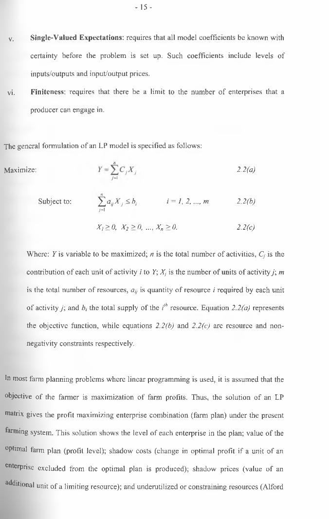
The general formulation of an LP model is specified as follows:
nMaximize: c ,X j
i =i2.2(a)
Subject to: '*EjaijX j < bi i = 1, 2, .... m7=1
2.2(b)
X,>0, X2 >0, ...,X„>0. 2.2(c)
Where: Y is variable to be maximized; n is the total number of activities, Cj is the
contribution of each unit of activity i to Y\ Xj is the number of units of activity j; m
is the total number of resources, % is quantity of resource i required by each unit
of activity j; and b, the total supply of the i'h resource. Equation 2.2(a) represents
the objective function, while equations 2.2(b) and 2.2(c) are resource and non
negativity constraints respectively.
In most farm planning problems where linear programming is used, it is assumed that the
objective of the farmer is maximization of farm profits. Thus, the solution of an LP
matrix gives the profit maximizing enterprise combination (farm plan) under the present
farming system. This solution shows the level of each enterprise in the plan; value of the
optimal farm plan (profit level); shadow costs (change in optimal profit if a unit of an
enterprise excluded from the optimal plan is produced); shadow prices (value of an
additional unit of a limiting resource); and underutilized or constraining resources (Alford
- 16 -
et al, 2004 and Babatunde et al, 2007). However, the major weakness of this technique is
its inability to account for risks, resulting in farm plans that do not represent a complete
picture of the (risky) farming environment (Ateng, 1977 and Rafsnider et al, 1993).
2.2.2 Quadratic Programming
The quadratic programming or quadratic risk programming (QRP) technique is based on
the expected utility and portfolio theories advanced by von-Neuman and Morgenstem
(1944) and Markowitz (1952) respectively. The expected utility theory is invoked in the
acknowledgement that risks inherent in agricultural production cause the income from a
farm activity to be stochastic, in which case it has an expected value E, equal to its mean
and a variance, V, which is a measure of risk. The portfolio theory, on the other hand
explains the rationale for enterprise diversification: due to the stochastic nature of income
from farm enterprises, farmers, being risk averse, diversify their enterprises in order to
minimize the variation of the expected income (Adams et al, 1980 and Crisostomo and
Featherstone, 1990).
QRP assumes that a farmer’s attitude to risk while choosing a farm plan depends on an
expected income-variance utility function (Thomson and Hazell, 1972 and Bhende, and
Venkataram, 1994), which Freund (1956) equated to the utility of net revenue (money). QRP
is therefore used to generate a set of efficient EV farm plans, which minimizes variances
associated with increasing levels of expected income (Rafsnider et al, 1993). The EV set
defines a utility maximizing frontier; on which each farmer’s optimal farm plan could be
found. The point on the frontier where utility is maximised is determined by the farmer’s
level of risk aversion (Rafsnider et al, 1993 and Bhende and Venkataram, 1994).
- 17 -
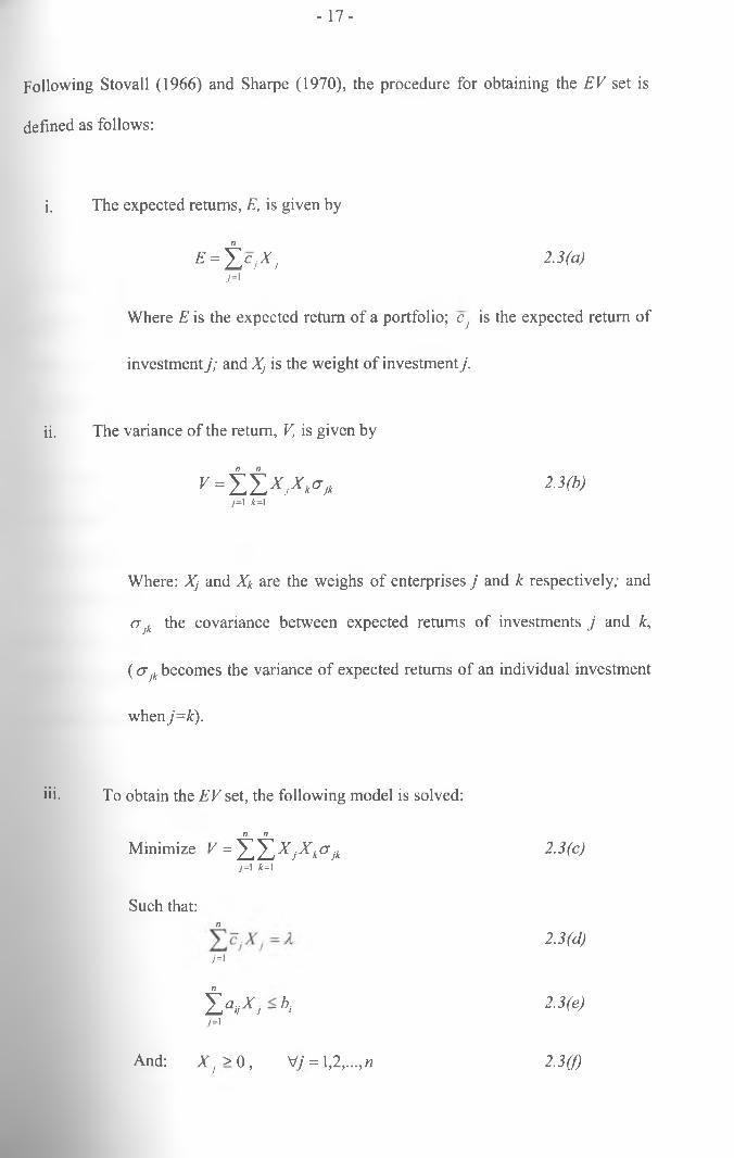
Following Stovall (1966) and Sharpe (1970), the procedure for obtaining the EV set is
defined as follows:
i. The expected returns, E, is given by
E = ± C j X j 2.3(a)J~ i
Where E is the expected return of a portfolio; cy is the expected return of
investment j; and Xj is the weight of investment j.
ii. The variance of the return, V, is given by
v = i . i . x ,x >°» Z3<b>7=1 *=1
Where: Xj and Xk are the weighs of enterprises j and k respectively; and
crjk the covariance between expected returns of investments j and k,
( a jk becomes the variance of expected returns of an individual investment
when j=k).
iii. To obtain the EV set, the following model is solved:
Minimize V = H X j X ^ 2.3(c)7=1 k =1
Such that:n
7=12.3(d)
' f h a i/X j ~ bi7=1
2.3(e)
And: X j> 0, V/ = 1,2.... w 2.3(f)
- 18 -
Where: A is a scalar equal to expected income, E, and represents the aspiration
level of the investor. Other variables are as defined in equations 2.2(a), 2.2(b),
2.2(c), 2.3(a) and 2.3(b).
The solution of the above QRP will give the levels of each investment in the portfolio that
minimize the variance of expected returns (efficient portfolio) for the level of expected
returns specified in the expected returns equation, and satisfy the other specified
constraints.
The EV model is has some strengths as well as weaknesses. For example, Harwood et al
(1999) find the expected utility theory advantageous in that it can accommodate a variety
of utility functions and probability distributions. But the authors also find the theory to be
weak in that utility functions are difficult to measure and the assumption that decision
makers are highly rational is not always true. Similarly, Nyikal and Kosura (2005)
identify a weakness in the portfolio theory in that not all investors can find their optimal
enterprise mix in the EV set.
- 19 -
2.3 A Review of Some Farm Planning Studies
Both LP and QRP have been widely applied in farm planning studies, a few of which
have been summarised in this section. In Pakistan, Ishtiaq et a/ (2005) studied cropping
patterns in irrigated areas of Punjab to determine optimal crop combinations and found
that the farmers were more or less operating at the optimal level. This was supported by
the fact that in the optimal solution, although there were changes in resource allocation to
the different crops, the overall cropped acreage decreased by only 0.37 percent; and
income increased by a paltry 1.57 percent compared to the existing acreage. But Adesiyan
et al (2007) studied the optimal maize-based enterprise combination of farmers in Orie
Local Government Area of Nigeria using linear programming and reported different
findings. The researchers concluded that farmers in the study area were not adopting
optimal farm plans, based on existing level of resources. They also concluded that
growing sole crops yielded more income than combining crops.
The results from these two studies imply that although farm planning may lead to
reallocation of resources, this may not always translate into significant increases in the
objective function (farm incomes). Further, according to these results, it cannot be
generalized that farmers are always misallocating resources. The above studies have
shown that some farmers are efficient, given the current level of resources and technology
available to them, in which case productivity can only be increased through technological
advancement and/or relaxation of resource constraints.
Among the early farm planning studies to incorporate risk was the one by Freund (1956).
Freund used quadratic programming to determine the optimum crop combination for a
representative farm in Eastern North Carolina under both ‘risk’ and ‘no-risk’ situations,
is results show that the high risk enterprises comprising potatoes and fall cabbage
- 2 0 -
accounted for 87.3 percent of the total net revenue in the ‘no-risk’ program, compared to
59 2 percent in the ‘risk’ program. Further, the less risky com enterprise featured
prominently in the ‘risk’ program, but was excluded in the ‘no-risk’ program. Overall, the
expected net revenue in the ‘no-risk’ program was about 26.7 percent more than that of
the ‘risk’ program.
Three decades later, Manos et al (1986) determined optimal farm plans for Central
Macedonia. The study results showed that the risk-efficient farm plan suggested by the
EV model generated using quadratic programming was different from the existing plan.
The area allocated to com, cotton to be picked by hand, sugar beet, and alfalfa increased
in the optimal plan whereas the area allocated to cotton to be picked by machine, barley,
tomatoes for processing, and beans decreased. In addition, EV model results suggested a
better use of the available family labour and invested capital; and about 20 per cent
increase profits.
Riaz (2002) used quadratic risk programming to determine optimal agricultural land use
systems for northern Pakistan. Among his main findings were that with subsistence
constraints, existing farm plans in the lower irrigated zone were equally as profit and risk-
efficient as the optimal plans; but without subsistence constraints, resource reallocation
could increase farmers’ income by 8-10 percent. This, according to Riaz, implied that in
the event of a disaster, farmers would be better-off having adopted the risk optimizing
tarm plan rather than the existing one. With subsistence constraint, the finding that
existing farm plans are optimal concurs with the linear programming study by Ishtiaq et
(2005), quoted earlier. However, this finding contradicts those of risk studies by
Freund (1956) and Manos et al (1986) above.
-21 -
Closer home, recent studies in the Africa continue to underscore the significance of risk
in farm planning. Fufa and Hassan (2006) used quadratic programming to assess income
risk and crop production patterns of small-scale farmers in Eastern Oromiya, Ethiopia.
They found out that as farmers become more risk averse, land allocated to maize was no
more than just enough to meet the subsistent requirement, due to high level of maize
income risk. On the other hand, the area allocated to sorghum production increased with
risk aversion, due to stable yield and income from the crop. Further, the risk-neutral
optimal farm plans (equivalent to those generated by linear programming) suggested the
highest values of both expected returns and risk.
Most recently, Msusa (2007) used QRP to investigate the production efficiency of
smallholder farmers in Malawi. His findings were that the variability of a crop
enterprise’s profitability, which is a measure of risk, significantly influenced the cropping
pattern adopted by a farmer. He concluded that farmers should increase land allocated to
groundnuts by about 198 per cent and decrease area under maize, tobacco and beans by
about 47, 69 and 78 percent respectively, in order to optimize risk.
In Kenya, a number of earlier farm planning studies were carried out using linear
programming, and provided insightful results on smallholder farmer resource allocation.
The study by Mukumbu (1987) on enterprise mix and resource allocation in West Kano
pilot irrigation scheme revealed that farmers could more than double their gross margins
by adopting optimal plans. This implies that the farmers were misallocating resources
through adoption of sub-optimal farm plans.
Similarly, Nguta (1992) studied resource allocation by smallholder irrigation farmers
al°ng the Yatta Canal of Machakos district and concluded that farmers were not efficient
- 22 -
in allocating their resources. His study suggested that farmers’ total gross margins could
increase by between 28 and 121 percent, if they reallocated their resources and adopted
the optimal farm plans. The study also found working capital to be limiting, with a
marginal value product that exceeded the average credit lending rates. This implied that it
was economically feasible for farmers to obtain credit to enable them invest in optimal
enterprise combinations.
Furthermore, Wanzala (1993) assessed the economic competitiveness and optimal
resource allocation among smallholder rain-fed rice producers in Busia district. The main
finding was that rice was excluded from optimal farm plans, although farmers included it
in their own cropping patterns. The implication was that farmers were misallocating their
resources and could raise their incomes by adopting the optimal farm plans.
These studies showed that farmers in many parts of Kenya grossly misallocate their
resources and could raise their productivity and farm incomes by adopting optimal farm
plans. The shortcoming of these studies however, was their assumption that farmers are
risk-neutral. The optimal plans generated did not allow farmers to choose plans that
match their levels of risk preference.
Recent studies in the country are however acknowledging the need to incorporate risk in
farm planning. Nyikal and Kosura (2005) used both linear and quadratic programming to
assess risk preference and optimal enterprise combinations among smallholder farmers in
Kahuro division of Murang’a district. The risk-neutral solution (produced using linear
programming) revealed an optimal farm plan without subsistence requirement that
featured 0.35 acres of coffee, 0.01 long rain sweet potatoes and 1.14 acres of banana; with
total gross margin of 34,171 Kenya Shillings. On the other hand the optimal farm plans
- 2 3 -
with subsistence requirement comprised of 0.31 acres of long rain maize and beans, 0.31
acres of short rain maize and beans, 0.34 acres of coffee, 0.38 acres of long rain sweet
potatoes, and 0.47 acres of bananas; giving a total gross margin of 30,097 Kenya
shillings. The conclusion was that the more risk aversive farm plans, which included
maize for subsistence, resulted in lower farm incomes than the less risk averse farm plans
which ignored a subsistence crop.
Further, the results of risk model (QRP) without subsistence constraint suggested that
high risk enterprises enter the optimal farm plan at high levels of risk, while low risk
enterprises dominated the farm plans at low risk levels. The optimal farm plans with
subsistence constraint yielded lower incomes for a given level of risk than without the
subsistence constraint. This notwithstanding, most farmers included the low income
subsistence crops, resulting in inefficient farm plans. The conclusion was that farmers
who are more risk averse allocated more resources to subsistence crop production and
earned lower incomes than the less risk averse farmers. Hence, farmer-preferred cropping
patterns were risk minimizing, not profit maximizing.
Similar findings were also reported by Diang’a (2006), who studied the effect of maize
price risk on smallholder agricultural production in Kakamega District. In the risk-neutral
model, the optimal farm plans yielded an income of Ksh 48,458 compared to existing
plans, which earned farmers an income of Ksh 28,238. This shows that farmers could
raise their incomes by 71.6 percent by adopting optimal production plans. On the other
hand, the QRP model for the average farm suggested an optimal total gross margin of Ksh
72,121, which was 155.4 percent above that of the existing farm plans. He further found
that farmers grew higher pay-off crops (which are also riskier to produce) only if their
risk aversion was low.
- 24 -
In co n clu sio n , results of the risk studies reviewed suggest that enterprise risk and farmers’
risk attitude affect the efficiency of smallholder farmer resource allocation, and
con seq u en tly expected returns. More often than not, farmers end up adopting farm plans
that minimise risk, but also give them lower than optimal farm incomes for the level of
risk assum ed. It follows therefore, that smallholder farmers in Kenya and indeed other
d evelop in g countries can increase their farm incomes by reallocating their resources to
adopt risk-efficient farm plans. The studies have further demonstrated that despite its few
w eak n esses, Q R P can be used to study how risks affect selection of optimal farm plans,
ju stify in g its use in this study.
- 25 -
Chapter 3: Methodology
This chapter presents the methodology used in the study. It covers the analytical
fram ew ork (theoretical and empirical frameworks), a brief description of the study area,
sources of data used, data collection methods, sample size and sampling procedures, and
data analysis procedures.
3.1. Theoretical Framework
This study was anchored broadly on the theory of the firm. According to this theory,
production decisions of a farmer are assumed to be driven by the desire to maximize
expected utility (or expected profit), subject to availability of production constraints such
as land, labour and capital (Feder et al, 1985). This profit is a function of the enterprises
that a farmer chooses to operate and the technologies that a farmer employs in production
of the selected enterprises.
To accommodate risk in the farmer’s utility maximization venture, two economic theories
specifically guided the study. These are the expected utility theory pioneered by von-
Neuman and Morgenstem (1944) and the portfolio theory founded on the work of
Markowitz (1952), as stated in Chapter 2. Under the expected utility theory, a farmer is
assumed to derive some cardinal utility from returns of investing in farming activities.
But given the risky nature of agriculture, the farmer will not always get the predicted
value of returns: there will be deviations (variance) from this value. With this in mind, the
farmer, being mostly risk averse, will invest in a combination of enterprises (called a
portfolio or a farm plan), in order to minimize the risk. This is the gist of the portfolio
theory, which presumes that the farmer is willing to choose among farm plans entirely on
- 26 -
the basis of predicted income (mean) and uncertainty (variance) of that income (Sharpe,
1970; Crisostomo and Featherstone, 1990; and Fufa and Hassan, 2006).
The objective of portfolio analysis is to find out a set of efficient farm plans and the
efficient frontier, which is the maximum mean return for a given level of variance, or the
minimum variance for a given mean return (Barkley and Peterson, 2008). A farm plan is
deemed more efficient than another if for the same expected return, its variance of return
is smaller, or if for the same level of variance of expected return, its expected return is
higher (Sharpe, 1970).
Following this efficiency criterion, a farmer’s decision is based on the following rules
according to Sharpe (1970):
1. The general rule is to choose the farm plan with a larger expected return and
smaller variance of return than another.
2. If two farm plans have the same expected returns and different variances of return,
the one with smaller variance of return is preferred.
3. If two farm plans have the same variance of return and different expected returns,
the one with larger expected return is preferred
Figure 3.1 illustrates how a risk averse farmer chooses a risk-efficient enterprise mix as
theorised by Harwood et al (1999) and Lien (2002). The farmer’s preferences are
represented by indifference curves U|, U2 and U3. Each curve connects a locus of risk
(represented by variance of expected income) and expected income levels that generate
the same level of utility to the farmer. On the other hand, the EV efficient frontier
connects locus of points that define the minimum variance associated with each level of
expected income. The farmer desires a high level of expected net farm income and a low
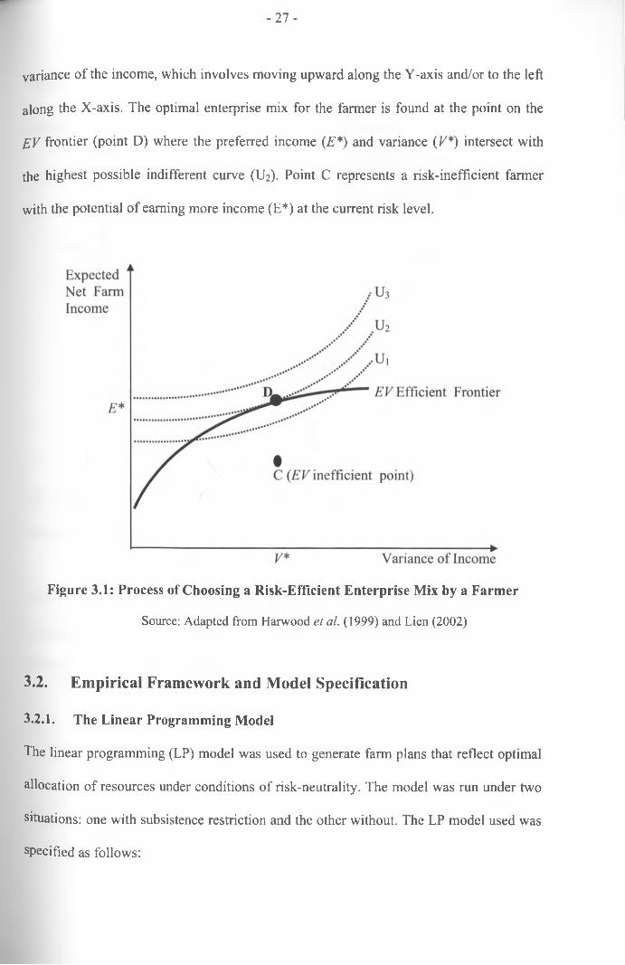
- 27 -
variance of the income, which involves moving upward along the Y-axis and/or to the left
along the X-axis. The optimal enterprise mix for the farmer is found at the point on the
EV frontier (point D) where the preferred income (E *) and variance (V*) intersect with
the highest possible indifferent curve (U2). Point C represents a risk-inefficient farmer
with the potential of earning more income (E*) at the current risk level.
Figure 3.1: Process of Choosing a Risk-Efficient Enterprise Mix by a Farmer
Source: Adapted from Harwood et al. (1999) and Lien (2002)
3.2. Empirical Framework and Model Specification
3.2.1. The Linear Programming Model
The linear programming (LP) model was used to generate farm plans that reflect optimal
allocation of resources under conditions of risk-neutrality. The model was run under two
situations: one with subsistence restriction and the other without. The LP model used was
specified as follows:
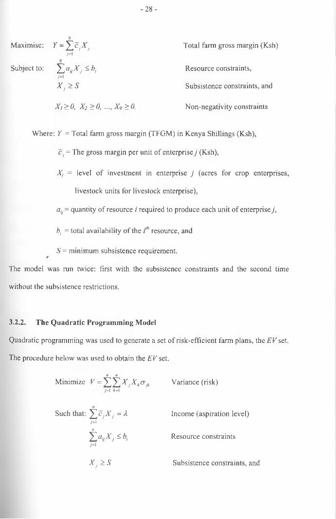
- 2 8 -
9Maximise: Y = ^ C jX j Total farm gross margin (Ksh)
9Subject to: ^ j aijX j <bi Resource constraints,
X j >S Subsistence constraints, and
X,>0, X2 >0, ...,X9 >0. Non-negativity constraints
Where: Y = Total farm gross margin (TFGM) in Kenya Shillings (Ksh),
Cj = The gross margin per unit of enterprise j (Ksh),
Xj = level of investment in enterprise j (acres for crop enterprises,
livestock units for livestock enterprise),
a:j = quantity of resource i required to produce each unit of enterprise j ,
b; = total availability of the i'h resource, and
S = minimum subsistence requirement.
The model was run twice: first with the subsistence constraints and the second time
without the subsistence restrictions.
3.2.2. The Quadratic Programming Model
Quadratic programming was used to generate a set of risk-efficient farm plans, the EV set.
The procedure below was used to obtain the EV set.
n nMinimize V = V V X jX ko jk Variance (risk)
7=1 *=1
nIncome (aspiration level)
n
Resource constraints
X j > S Subsistence constraints, and
- 2 9 -
X t > 0, X 2 > 0,..., X g > 0 Non-negativity constraints
Where:
V = Total variance associated with income level E (Ksh)
Xj,Xk = units of production allocated to enterprises j and k respectively
crjk = covariance between expected returns of enterprises j and k,
(variance of expected returns of an individual enterprise when j=k).
All other notations are as defined in the LP equations in section 3.2.1.
Like the LP model, the QRP model was also solved with and without the subsistence
constraints. The EV set was generated by setting A at some arbitrary low level and
successively raising it by Ksh 1,000, until the solution became infeasible. This approach
has been adopted in a number of studies (see for example, Stovall, 1966, and Barkley and
Peterson, 2008). The last feasible solution was deemed to give the maximum risk-
efficient income, and risk-efficient farm plan.
3.2.3. Model Activities and Constraints
3.2.3.1. Real Activities (Enterprises)
Nine major activities were identified. These were:
1) Maize 1 (Mzel) - maize grown in short rains. This enterprise consists mainly
of maize, intercropped with beans and peas;
2) Maize2 (Mze2) - maize grown in long rains. This enterprise consists mainly
of maize, intercropped with beans and peas;
3) Coffee (Coff) - coffee, grown in short and long rain seasons;
4) French Beans 1 (Fbnl) - French beans grown in short rains;
5) Kales 1 (Kal 1) - Kales grown in short rains;
- 30 -
6) Kales2 (Kal2) - Kales grown in long rains;
7) Tomato 1 (Tom 1) - Tomatoes grown in short rains;
8) Totmato2 (Tom2) - Tomatoes grown in long rains;
9) Livestock (Lvst) - cattle and shoats, kept in both long and short rain seasons.
3.2.3.2. Model Constraints
A total of 12 constraints, summarized in table 3.2(b) were identified. The constraints were
specified as follows:
i. Irrigable land - represents average irrigable land per household. Its calculation
was based on quantity of water that farmers can comfortably use from the dam for
irrigation during the dry spell when water is limiting. This land has two seasonal
constraints df 0.250 acres each6. Irrigable land is assumed to be used for
horticultural crops only (most farmers irrigate horticultural crops only).
ii. Non-irrigable land - this represents the average size of land that could not be
irrigated due to water availability constraints. It was calculated as average
cultivable land (1.268 acres) less irrigable land. Non-irrigable land had two
seasonal constraints of 1.018 acres each.
iii. Family Labour - This was calculated using the number and availability of
household members. Owing to differences in age among family members, the
weights adopted by Nguta (1992) were used to convert household members into
standard labour units (man equivalents), as presented in table 3.2(a). One man day
was considered to consist of 8 working hours. Each month had 26 working days,
Acres were used instead o f hectares because land holdings in the study area are very small and also the acre is the most commonly used unit of land measurement in the area (2.5acres = 1 hectare).
-31 -
except for December, which had 24 working days due to Christmas and Boxing
Day holidays. Male labour was not distinguished from female labour, because
there was no indication that farmers categorized labour on the basis of gender.
Two family labour constraints of 397 man days in short rain season and 434 man
days in long rain season were identified.
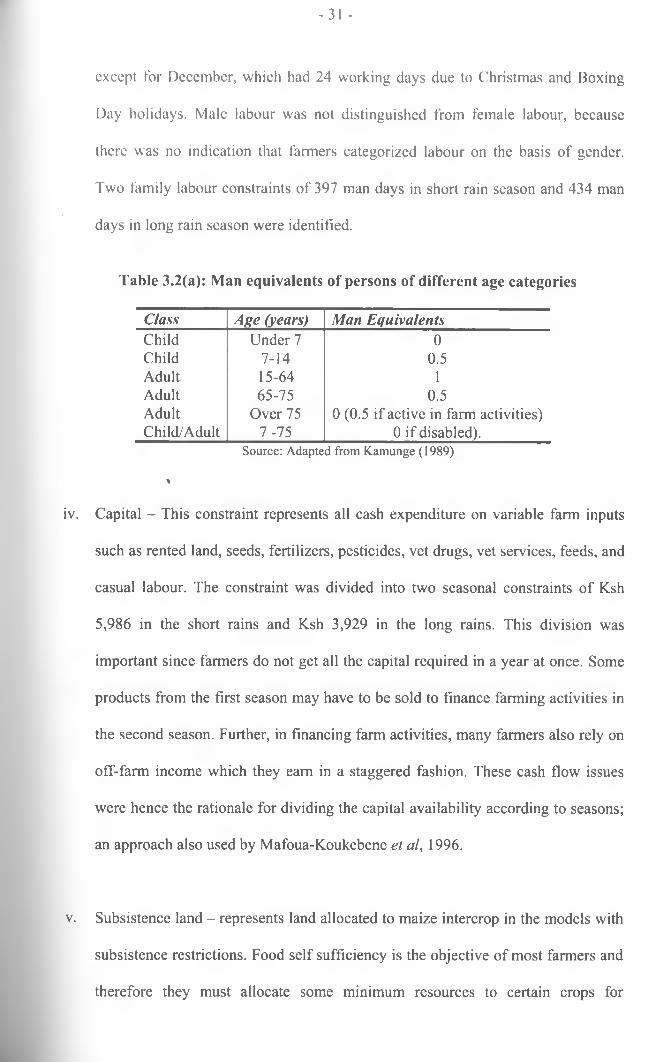
Table 3.2(a): Man equivalents of persons of different age categories
Class Age (years) Man EquivalentsChild Under 7 0Child 7-14 0.5Adult 15-64 1Adult 65-75 0.5Adult Over 75 0 (0.5 if active in farm activities)Child/Adult 7-75 0 if disabled).
Source: Adapted from Kamunge (1989)
%
iv. Capital - This constraint represents all cash expenditure on variable farm inputs
such as rented land, seeds, fertilizers, pesticides, vet drugs, vet services, feeds, and
casual labour. The constraint was divided into two seasonal constraints of Ksh
5,986 in the short rains and Ksh 3,929 in the long rains. This division was
important since farmers do not get all the capital required in a year at once. Some
products from the first season may have to be sold to finance farming activities in
the second season. Further, in financing farm activities, many farmers also rely on
off-farm income which they earn in a staggered fashion. These cash flow issues
were hence the rationale for dividing the capital availability according to seasons;
an approach also used by Mafoua-Koukebene et al, 1996.
v. Subsistence land - represents land allocated to maize intercrop in the models with
subsistence restrictions. Food self sufficiency is the objective of most farmers and
therefore they must allocate some minimum resources to certain crops for
- 32 -
subsistence. Riaz (2002), N yikal and Kosura (2005) and Kitoo (2008) link
inclusion of subsistence crops in farmer plans to not only meeting subsistence
needs but also reducing risk associated with food markets. For this reason,
inclusion of some minimum resources for subsistence makes a farm plan more
rational to smallholder farmers.
Maize is the main staple crop in the study area, while less than 20 percent of the
main horticultural crops is used for home consumption (see Section 4.1.1),
meaning that the crops are not grown primarily for subsistence. Maize was hence
the only crop to which the subsistence constraint was allocated. The minimum
subsistertce land requirement was calculated using a per capita maize requirement
of 103 kg per year (De Groote et al, 2002). This approach is also popular in
Kenyan farm planning studies (see Nguta, 1992 and Nyikal and Kosura, 2005).
The annual maize requirement for a 6-member household was 618 kg. With the
mean maize yield in the study area being 406 kg per acre per season, each
household had two subsistence land constraints, measuring 0.761 acres each.
vi. Subsistence carrying capacity - this represents livestock units required for
‘subsistence’. Mostly, farmers in the area keep livestock for needs that seem to
fulfil a complex subsistence objective. This objective covers subsistence demand
for milk and manure, cultural value, store of wealth, and a quick source of cash for
financing farm inputs and operations and other family needs, including
emergencies. Hence, the livestock enterprise plays a crucial role not only for
subsistence, but also in cushioning farmers against risks. To account for this
objective, the existing mean stocking rate of 1.3 livestock units (LU) per acre of
cultivable land was used to derive the livestock carrying capacity allocated for
- 33 -
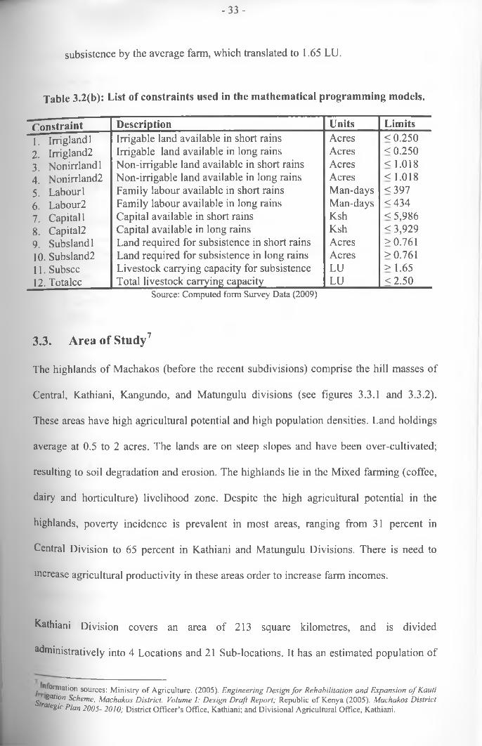
subsistence by the average farm, which translated to 1.65 LU.
Table 3.2(b): List of constraints used in the mathematical programming models.
Constraint Description Units Limits1. Irriglandl Irrigable land available in short rains Acres <0.2502. Irrigland2 Irrigable land available in long rains Acres < 0.2503. Nonirrlandl Non-irrigable land available in short rains Acres < 1.0184. Nonirrland2 Non-irrigable land available in long rains Acres < 1.0185. Labour 1 Family labour available in short rains Man-days <3976. Labour2 Family labour available in long rains Man-days <4347. Capital 1 Capital available in short rains Ksh < 5,9868. Capital2 Capital available in long rains Ksh < 3,9299. Subslandl Land required for subsistence in short rains Acres >0.76110. Subsland2 Land required for subsistence in long rains Acres >0.76111. Subscc Livestock carrying capacity for subsistence LU > 1.6512. Totalcc Total livestock carrying capacity LU <2.50
Source: Computed form Survey Data (2009)
3.3. Area of Study7
The highlands of Machakos (before the recent subdivisions) comprise the hill masses of
Central, Kathiani, Kangundo, and Matungulu divisions (see figures 3.3.1 and 3.3.2).
These areas have high agricultural potential and high population densities. Land holdings
average at 0.5 to 2 acres. The lands are on steep slopes and have been over-cultivated;
resulting to soil degradation and erosion. The highlands lie in the Mixed farming (coffee,
dairy and horticulture) livelihood zone. Despite the high agricultural potential in the
highlands, poverty incidence is prevalent in most areas, ranging from 31 percent in
Central Division to 65 percent in Kathiani and Matungulu Divisions. There is need to
increase agricultural productivity in these areas order to increase farm incomes.
Kathiani Division covers an area of 213 square kilometres, and is divided
administratively into 4 Locations and 21 Sub-locations. It has an estimated population of
j n °nnation sources: Ministry of Agriculture. (2005). Engineering Design for Rehabilitation and Expansion o f Kauti Str^al‘° n ^c^eme‘ Machakos District. Volume I: Design Draft Report; Republic of Kenya (2005). Machakos District
a,egic Plan 2005- 2010; District Officer’s Office, Kathiani; and Divisional Agricultural Office, Kathiani.
- 34 -
122,347 persons in 24,471 households, and is the second most densely populated division
in Machakos, with 574 persons per square kilometre. The main economic activity in the
Division is Agriculture. Most of the farming is rain-fed, but a few farmers practice
irrigation to supplement rainfall. The Division has 10 small scale farmer-managed
irrigation schemes, most of which are currently being expanded or rehabilitated. Table
3.3.2 shows the administrative units and population data of Kathiani Division.
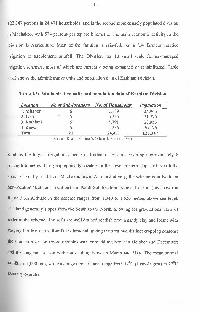
Table 3.3: Administrative units and population data of Kathiani Division
Location No o f Sub-locations No. o f Households Population1. Mitaboni 6 7,189 35,9432. Iveti 5 6,255 31,2753. Kathiani 5 5,791 28,9534. Kaewa 5 5,236 26,176Total 21 24,471 122,347
Source: District Officer’s Office, Kathiani (2009)
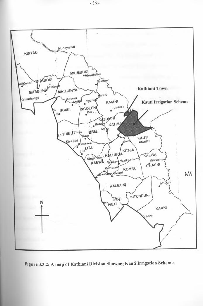
Kauti is the largest irrigation scheme in Kathiani Division, covering approximately 8
square kilometres. It is geographically located on the lower eastern slopes of Iveti hills,
about 24 km by road from Machakos town. Administratively, the scheme is in Kathiani
Sub-location (Kathiani Location) and Kauti Sub-location (Kaewa Location) as shown in
figure 3.3.2.Altitude in the scheme ranges from 1,340 to 1,620 metres above sea level.
The land generally slopes from the South to the North, allowing for gravitational flow of
water in the scheme. The soils are well drained reddish brown sandy clay and loams with
varying fertility status. Rainfall is bimodal, giving the area two distinct cropping seasons:
the short rain season (more reliable) with rains falling between October and December;
and the long rain season with rains falling between March and May. The mean annual
rainfall is 1,000 mm, while average temperatures range from 12°C (June-August) to 22°C
(January-March).
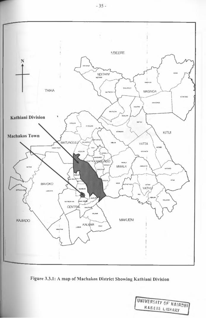
Figure 3.3.1: A map of Machakos District Showing Kathiani Division
- 36 -
Figure 3.3.2: A map of Kathiani Division Showing Kauti Irrigation Scheme
- 37 -
3.4. Data Types, Sources and Collection
The study used primary data since secondary data of individual farmers were not%
available at a central place. The data were collected in March 2009, through a farm
household survey and a focus group discussion (FGD). The survey covered 2007/08 short
rain and 2008 long rain seasons. The FGD was held with farmers prior to the survey. The
meeting served three purposes. First, it was used as a sensitization meeting for farmers
about the upcoming survey. Second, it was a tool for gaining insights into the general
socio-cultural and agricultural background of the residents of the study area. Thirdly, the
meeting generated additional information for both the survey and questionnaire design.
More details about the issues discussed during the meeting are contained in the focus
group discussion schedule in Appendix 1.
Primary data were collected on household characteristics (number, gender, age, education
level and occupation and of household members); characteristics of the household head
(gender, age, farming experience, education level and occupation); farm enterprise
characteristics (farm size and farm assets; crops grown including areas planted and the
cropping patterns; livestock kept including their types, numbers and production systems;
inputs used: manure, fertilizer, seed, feeds, labour and pesticides, including their types
and quantities; crop and livestock outputs including their quantities and utilization; and
product and input marketing including prices and marketing channels). The survey data
was collected using a pre-tested, structured questionnaire (see appendix 2), administered
to respondents by trained enumerators.
- 38 -
3.5. Sampling Procedure and Sample Size
Two main sampling methods were used in the study: purposive sampling and probability
proportional to size (PPS) sampling. Purposive sampling was used to select the study site
(district, division and the irrigation scheme). Machakos District was selected because it
represents the semi-arid districts in Kenya with high agricultural potential. Kathiani
Division was selected due to its high poverty incidence among the densely populated
divisions of Machakos, while Kauti Irrigation scheme was selected due to its large size
(in terms of number of farmers) compared to other schemes in the Division. An irrigation
scheme was preferred since most high value enterprises and farming systems being
promoted in the area require irrigation to supplement rainfall and there is deliberate
government support in irrigation projects.
According to Yansaneh (2005), PPS is a preferred methodology in most rural household
surveys due to its ability to improve the precision of the survey estimates. The method
was used in this study to select households to be interviewed. However, its limitation is
that it requires a prior knowledge of the population size in each primary sampling unit
(village in this case); yet accurate population data at such levels is not available in many
areas of Kenya.
Although the precise number of households or a list of all households in the Scheme was
not available, the boundaries of the Scheme are well known. The help of local Assistant
Chiefs and Village Headmen was enlisted to prepare a list of all households in the
scheme, stratified by village. This list constituted the sampling frame.
One hundred and twenty seven households, distributed proportionately to the village sizes
^n terms of population), were sampled as shown in Table 3.5. The sample size was
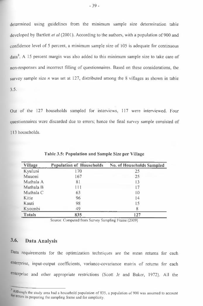
- 39 -
determined using guidelines from the minimum sample size determination table
developed by Bartlett et al (2001). According to the authors, with a population of 900 and
confidence level of 5 percent, a minimum sample size of 105 is adequate for continuous
data8. A 15 percent margin was also added to this minimum sample size to take care of
non-responses and incorrect filling of questionnaires. Based on these considerations, the
survey sample size n was set at 127, distributed among the 8 villages as shown in table
3.5.
Out of the 127 households sampled for interviews, 117 were interviewed. Four
questionnaires were discarded due to errors; hence the final survey sample consisted of
113 households.
Table 3.5: Population and Sample Size per Village
Village Population of Households No. of Households SampledKyuluni 170 25Muuoni 167 25Muthala A 81 13Muthala B 111 17Muthala C 63 10Kitie 96 14Kauti 98 15Kyoimbi 49 8Totals 835 127
Source: Computed from Survey Sampling Frame (2009)
3.6. Data Analysis
Data requirements for the optimization techniques are the mean returns for each
enterprise, input-output coefficients, variance-covariance matrix of returns for each
enterprise and other appropriate restrictions (Scott Jr and Baker, 1972). All the
^Although the study area had a household population of 835, a population of 900 was assumed to account errors in preparing the sampling frame and for simplicity.
- 4 0 -
coefficients and resource constraints were entered into the models as averages of the
sample data, having been calculated with the Statistical Package for Social Sciences
(SPSS) software. The ideal coefficients would have been sourced from experimental
stations, but Ateng (1977) notes that survey data are more reflective of actual smallholder
farm situation than experimental data.
Enterprise gross margins were used to represent enterprise returns. The gross margins
were calculated by subtracting total variable cost of production from value of total output
produced by the enterprise9. For crop enterprises, the value of output was calculated for
individual farmers by multiplying the total yields by average price faced by each farmer.
Non-marketed output was valued using the average price of marketed output. Costs of
production were also calculated using prices and quantities of inputs faced by individual
farmers. For the livestock enterprise, the animals were treated as capital stock, hence
only increases in their value together with physical outputs (milk and manure) were
considered in calculating gross margins. The gross margin was calculated using
guidelines proposed by Millear, et al (2005) as shown in appendix 3.
Gross margin for each enterprise was first calculated per farm then divided by land area
(livestock units for livestock) allocated to the enterprise to get gross margin per unit. The
per unit gross margins of each enterprise were then averaged over the number of farmers
running the enterprise to obtain the mean gross margins for the enterprises. All outputs
and inputs were valued in Kenya Shilling (Ksh). Input-output coefficients and subsistence
restrictions were calculated as averages of survey data using SPSS, as discussed in section
For each enterprise, the gross margin assumes that in the equation Gross Margin = Total Revenue (TR) - °tal Variable Cost (TVC) - Total Fixed Cost (TFC). TFC are not attributable and thus ignored for
convenience, hence, GM = TR-TVC.
-41 -
3.2.3 above. The variance-covariance matrix of enterprise gross margins (table 4.1.3(b)
was calculated using SPSS and entered into the QRP as a table.
To generate the optimal farm plans, a three situation analytical framework was used in
generating the optimal plans. First, maximising farmers’ total farm gross margin (TFGM)
subject to resource constraints and subsistence requirements (Risk-neutral subsistence
model); second, maximising TFGM subject to resource constraints (Risk-neutral non
subsistence model); and third, maximising farm income subject to risk and subsistence
requirements (Subsistence model with risk). Situations one and two were analysed using
an LP model, while situation three was analysed using a QRP model. The suitability of
LP and QRP for this kind of analysis is also acknowledged by Thomson and Hazell, 1972
and Nyikal and Kosura, 2005).
The optimisation models were solved using the General Algebraic Modelling System
(GAMS) computer program. The software is a powerful tool for formulating and solving
mathematical programming models such as linear programming, mixed integer
programming, quadratically constrained programming, mixed complementary and
stochastic linear programming. GAMS has been used in a number of recent risk
optimization studies10 and was therefore deemed appropriate for this study.
3.7. Hypothesis Testing
The first hypothesis was tested using the one sample location test, an application of the
student’s t-test (Wikipedia, 2009). This test was used to compare the mean total gross
Margin from the existing farm plan to a ‘known’ constant, equal to the total gross margin
°f the optimal farm plan.
U)"c ~ I&ee Nyikal and Kosura (2005); Diang’a (2006); Fufa and Hassan (2006); and Kitoo (2008).
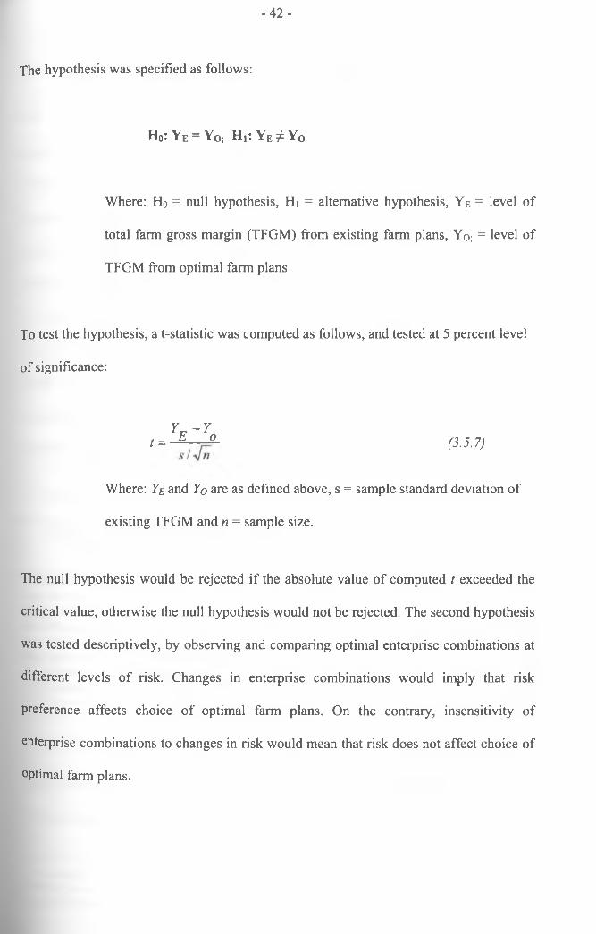
- 4 2 -
The hypothesis was specified as follows:
H0: Ye = Y0; H,: Ye^Y o
Where: Ho = null hypothesis, Hi = alternative hypothesis, Ye = level of
total farm gross margin (TFGM) from existing farm plans, Yo; = level of
TFGM from optimal farm plans
To test the hypothesis, a t-statistic was computed as follows, and tested at 5 percent level
of significance:
t =Y - - Y E o (3.5.7)
Where: Ye and Yo are as defined above, s = sample standard deviation of
existing TFGM and n = sample size.
The null hypothesis would be rejected if the absolute value of computed t exceeded the
critical value, otherwise the null hypothesis would not be rejected. The second hypothesis
was tested descriptively, by observing and comparing optimal enterprise combinations at
different levels of risk. Changes in enterprise combinations would imply that risk
preference affects choice of optimal farm plans. On the contrary, insensitivity of
enterprise combinations to changes in risk would mean that risk does not affect choice of
optimal farm plans.
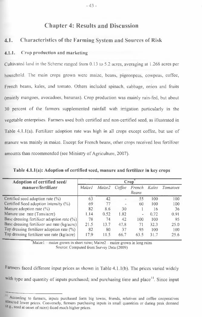
-43 -
Chapter 4: Results and Discussion
4.1. Characteristics of the Farming System and Sources of Risk
4.1.1. Crop production and marketing
Cultivated land in the Scheme ranged from 0.13 to 5.2 acres, averaging at 1.268 acres per
household. The main crops grown were maize, beans, pigeonpeas, cowpeas, coffee,
French beans, kales, and tomato. Others included spinach, cabbage, onion and fruits
(mainly mangoes, avocadoes, bananas). Crop production was mainly rain-fed, but about
30 percent of the farmers supplemented rainfall with irrigation particularly in the
vegetable enterprises. Farmers used both certified and non-certified seed, as illustrated in
Table 4.1.1(a). Fertilizer adoption rate was high in all crops except coffee, but use of
manure was mainly in maize. Except for French beans, other crops received less fertilizer
amounts than recommended (see Ministry of Agriculture, 2007).
Table 4.1.1(a): Adoption of certified seed, manure and fertilizer in key crops
Adoption of certified seed/ manure/fertilizer
CropM a ize l M aize2 C offee F rench
B eansK a les T om atoes
Certified seed adoption rate (%) 63 42 - 55 100 100Certified Seed adoption intensity (%) 69 77 - 60 100 100Manure adoption rate (%) 82 8.6 30 1 16 36Manure use rate (Tons/acre) 1.14 0.52 1.82 - 0.72 0.91Base dressing fertilizer adoption rate (%) 78 74 42 100 100 95Base dressing fertilizer use rate (kg/acre) 21.5 13.7 47.8 71 32.3 25.0Top dressing fertilizer adoption rate (%) 82 80 37 95 100 100Top dressing fertilizer use rate (kg/acre) 17.9 11.5 66.7 63.5 31.7 25.6
Maize 1 - maize grown in short rains; Maize2 - maize grown in long rains Source: Computed from Survey Data (2009)
Farmers faced different input prices as shown in Table 4.1.1(b). The prices varied widely
with type and quantity of inputs purchased; and purchasing time and place". Since input
According to farmers, inputs purchased form big towns, friends, relatives and coffee cooperatives attracted lower prices. Conversely, farmers purchasing inputs in small quantities or during peak demand te-g-, seed at onset o f rains) faced much higher prices.
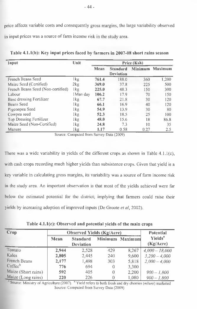
- 4 4 -
price affects variable costs and consequently gross margins, the large variability observed
in input prices was a source of farm income risk in the study area.
Table 4.1.1(b): Key input prices faced by farmers in 2007-08 short rains season
Input UnitMean
PriceStandardDeviation
(Ksh)Minimum Maximum
French Beans Seed 1kg 761.4 188.0 360 1,200Maize Seed (Certified) 2kg 369.0 37.8 225 500French Beans Seed (Non-certified) 1kg 225.0 48.3 150 300Labour 1 Man day 106.2 17.9 70 150Base dressing Fertilizer 1kg 67.7 21.8 30 120Beans Seed 1kg 66.1 16.9 40 120Pigeonpea Seed 1kg 54.9 13.9 30 80Cowpea seed 1kg 52.3 18.5 25 100Top Dressing Fertilizer 1kg 48.0 15.6 18 86.8Maize Seed (Non-Certified) 1kg 24.8 7.3 10 35Manure 1kg 1.17 0.58 0.27 2.5
Source: Computed from Survey Data (2009)
There was a wide variability in yields of the different crops as shown in Table 4.1.1(c),
with cash crops recording much higher yields than subsistence crops. Given that yield is a
key variable in calculating gross margins, its variability was a source of farm income risk
in the study area. An important observation is that most of the yields achieved were far
below the estimated potential for the district; implying that farmers could raise their
yields by increasing adoption of improved inputs (De Groote et al, 2002).
Table 4.1.1(c): Observed and potential yields of the main crops
Crop Observed Yields (Kg/Acre) PotentialYields3
(Kg/Acre)Mean Standard
DeviationMinimum Maximum
Tomato 2,944 2,528 429 8,267 4,000-18,000Kales 2,805 2,445 240 9,600 3,200-4,000French Beans 2,177 1,498 303 5,818 2,000-4,000Coffeeb 776 694 0 3,300Maize (Short rains) 592 405 0 2,200 900-1,800
_ Maize (Long rains) 220 226 0 1,080 900-1,800Source: Ministry o f Agriculture (2007). b Yield refers to both fresh and dry cherries (mbuni) marketed
Source: Computed from Survey Data (2009)
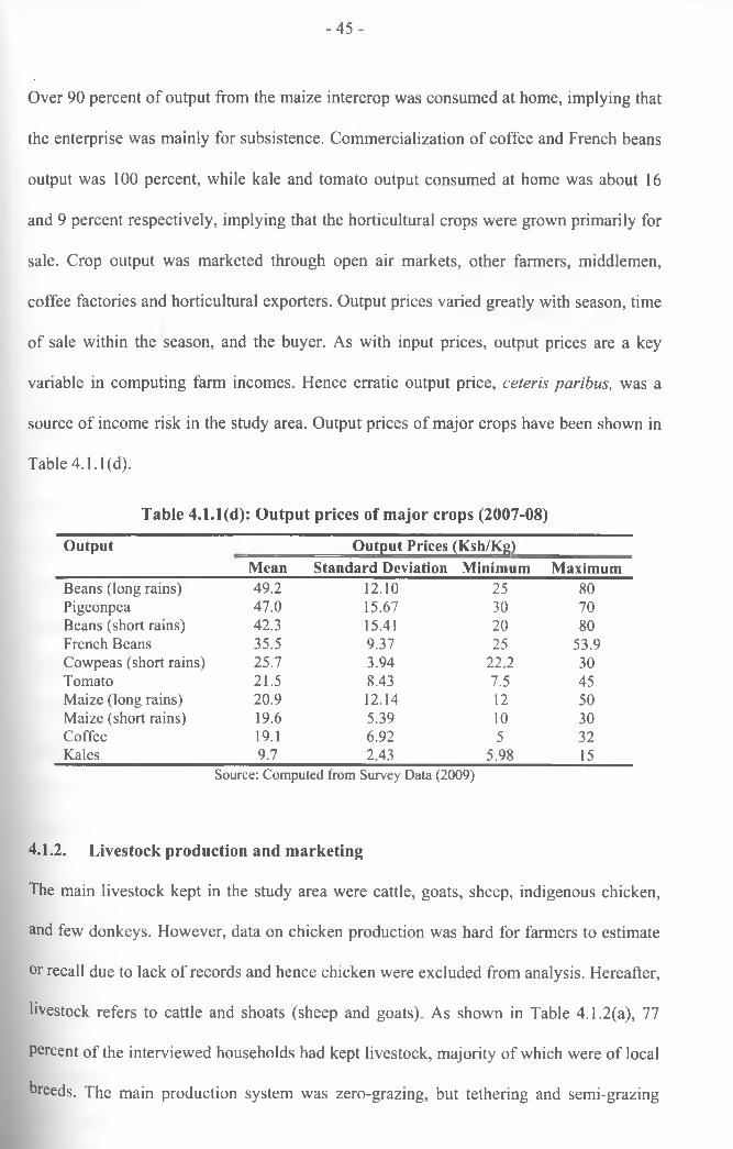
-45 -
Over 90 percent of output from the maize intercrop was consumed at home, implying that
the enterprise was mainly for subsistence. Commercialization of coffee and French beans
output was 100 percent, while kale and tomato output consumed at home was about 16
and 9 percent respectively, implying that the horticultural crops were grown primarily for
sale. Crop output was marketed through open air markets, other farmers, middlemen,
coffee factories and horticultural exporters. Output prices varied greatly with season, time
of sale within the season, and the buyer. As with input prices, output prices are a key
variable in computing farm incomes. Hence erratic output price, ceteris paribus, was a
source of income risk in the study area. Output prices of major crops have been shown in
Table 4.1.1(d).
Table 4.1.1(d): Output prices of major crops (2007-08)
Output Output Prices (Ksh/Kg)Mean Standard Deviation Minimum Maximum
Beans (long rains) 49.2 12.10 25 80Pigeonpea 47.0 15.67 30 70Beans (short rains) 42.3 15.41 20 80French Beans 35.5 9.37 25 53.9Cowpeas (short rains) 25.7 3.94 22.2 30Tomato 21.5 8.43 7.5 45M aize (long rains) 20.9 12.14 12 50M aize (short rains) 19.6 5.39 10 30Coffee 19.1 6.92 5 32Kales 9.7 2.43 5.98 15
Source: Computed from Survey Data (2009)
4.1.2. Livestock production and marketing
The main livestock kept in the study area were cattle, goats, sheep, indigenous chicken,
and few donkeys. However, data on chicken production was hard for farmers to estimate
or recall due to lack of records and hence chicken were excluded from analysis. Hereafter,
livestock refers to cattle and shoats (sheep and goats). As shown in Table 4.1.2(a), 77
percent of the interviewed households had kept livestock, majority of which were of local
breeds. The main production system was zero-grazing, but tethering and semi-grazing
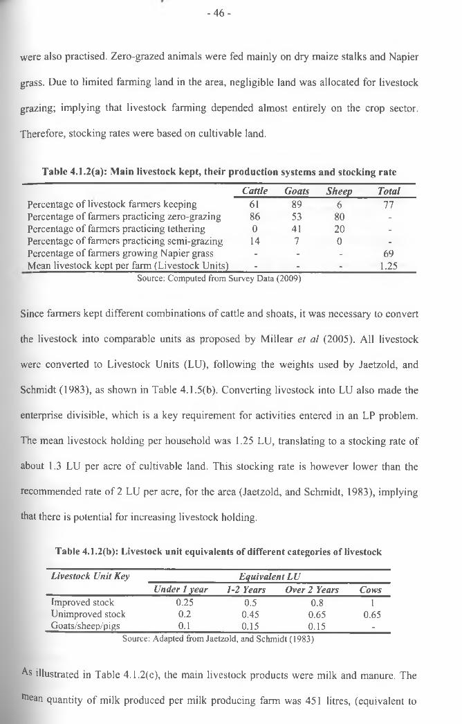
- 4 6 -
were also practised. Zero-grazed animals were fed mainly on dry maize stalks and Napier
grass. Due to limited farming land in the area, negligible land was allocated for livestock
grazing; implying that livestock farming depended almost entirely on the crop sector.
Therefore, stocking rates were based on cultivable land.
Table 4.1.2(a): Main livestock kept, their production systems and stocking rate
Cattle Goats Sheep TotalPercentage of livestock farmers keeping 61 89 6 77Percentage of farmers practicing zero-grazing 86 53 80 -Percentage of farmers practicing tethering 0 41 20 -Percentage of farmers practicing semi-grazing 14 7 0 -Percentage of farmers growing Napier grass - - - 69Mean livestock kept per farm (Livestock Units) - - - 1.25
Source: Computed from Survey Data (2009)
Since farmers kept different combinations of cattle and shoats, it was necessary to convert
the livestock into comparable units as proposed by Millear et al (2005). All livestock
were converted to Livestock Units (LU), following the weights used by Jaetzold, and
Schmidt (1983), as shown in Table 4.1.5(b). Converting livestock into LU also made the
enterprise divisible, which is a key requirement for activities entered in an LP problem.
The mean livestock holding per household was 1.25 LU, translating to a stocking rate of
about 1.3 LU per acre of cultivable land. This stocking rate is however lower than the
recommended rate of 2 LU per acre, for the area (Jaetzold, and Schmidt, 1983), implying
that there is potential for increasing livestock holding.
Table 4.1.2(b): Livestock unit equivalents of different categories of livestock
Livestock Unit Key Equivalent LUUnder 1 year 1-2 Years Over 2 Years Cows
Improved stock 0.25 0.5 0.8 1Unimproved stock 0.2 0.45 0.65 0.65Goats/sheep/pigs 0.1 0.15 0.15 -
Source: Adapted from Jaetzold, and Schmidt (1983)
As illustrated in Table 4.1.2(c), the main livestock products were milk and manure. The
ttiean quantity of milk produced per milk producing farm was 451 litres, (equivalent to
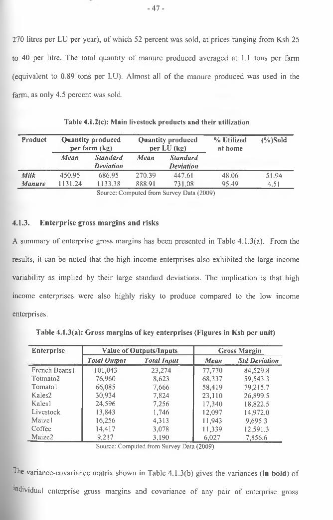
- 4 7 -
270 litres per LU per year), of which 52 percent was sold, at prices ranging from Ksh 25
to 40 per litre. The total quantity of manure produced averaged at 1.1 tons per farm
(equivalent to 0.89 tons per LU). Almost all of the manure produced was used in the
farm, as only 4.5 percent was sold.
Table 4.1.2(c): Main livestock products and their utilization
Product Quantity produced per farm (kg)
Quantity produced per LU (kg)
% Utilized at home
(%)Sold
Mean Standard Mean StandardDeviation Deviation
Milk 450.95 686.95 270.39 447.61 48.06 51.94Manure 1131.24 1133.38 888.91 731.08 95.49 4.51
Source: Computed from Survey Data (2009)
4.1.3. Enterprise gross margins and risks
A summary of enterprise gross margins has been presented in Table 4.1.3(a). From the
results, it can be noted that the high income enterprises also exhibited the large income
variability as implied by their large standard deviations. The implication is that high
income enterprises were also highly risky to produce compared to the low income
enterprises.
Table 4.1.3(a): Gross margins of key enterprises (Figures in Ksh per unit)
Enterprise Value of Outputs/Inputs Gross MarginTotal Output Total Input Mean Std Deviation
French Beans 1 101,043 23,274 77,770 84,529.8Totmato2 76,960 8,623 68,337 59,543.3Tomato 1 66,085 7,666 58,419 79,215.7Kales2 30,934 7,824 23,110 26,899.5Kales 1 24,596 7,256 17,340 18,822.5Livestock 13,843 1,746 12,097 14,972.0M aize 1 16,256 4,313 11,943 9,695.3C offee 14,417 3,078 11,339 12,591.3M aize2 9,217 3,190 6,027 7,856.6
Source: Computed from Survey Data (2009)
The variance-covariance matrix shown in Table 4.1.3(b) gives the variances (in bold) of
mdividual enterprise gross margins and covariance of any pair of enterprise gross
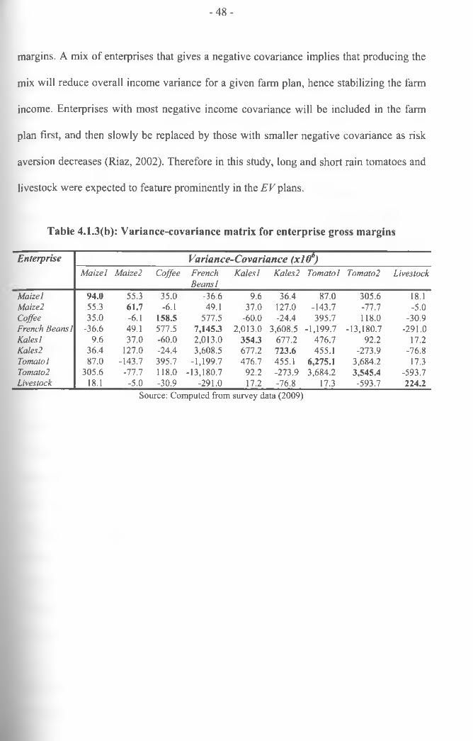
- 4 8 -
margins. A mix of enterprises that gives a negative covariance implies that producing the
mix will reduce overall income variance for a given farm plan, hence stabilizing the farm
income. Enterprises with most negative income covariance will be included in the farm
plan first, and then slowly be replaced by those with smaller negative covariance as risk
aversion decreases (Riaz, 2002). Therefore in this study, long and short rain tomatoes and
livestock were expected to feature prominently in the EV plans.
Table 4.1.3(b): Variance-covariance matrix for enterprise gross margins
E n terp rise Variance-Covariance (xlO6)M aizel Maize2 Coffee French
Beans 1K a lesl Kales2 Tomato 1 Tomato2 Livestock
M aizel 94.0 55.3 35.0 -36.6 9.6 36.4 87.0 305.6 18.1Maize2 55.3 61.7 -6.1 49.1 37.0 127.0 -143.7 -77.7 -5.0Coffee 35.0 -6.1 158.5 577.5 -60.0 -24.4 395.7 118.0 -30.9French Beans 1 -36.6 49.1 577.5 7,145.3 2,013.0 3,608.5 -1,199.7 -13,180.7 -291.0K alesl 9.6 37.0 -60.0 2,013.0 354.3 677.2 476.7 92.2 17.2Kales2 36.4 127.0 -24.4 3,608.5 677.2 723.6 455.1 -273.9 -76.8Tomato 1 87.0 -143.7 395.7 -1,199.7 476.7 455.1 6,275.1 3,684.2 17.3Tomato2 305.6 -77.7 118.0 -13,180.7 92.2 -273.9 3,684.2 3,545.4 -593.7Livestock 18.1 -5.0 -30.9 -291.0 17.2 -76.8 17.3 -593.7 224.2
Source: Computed from survey data (2009)
- 4 9 -
4.2. Optimizing the Farm Plans
4.2.1. Risk-neutral farm plans
Results of the risk-neutral farm plans for the average farm with 1.268 acres of cultivable
land have been presented in Tables 4.2.1(a) and 4.2.1(b). The results in Table 4.2.1(a)
show that with subsistence constraints, the farmer should allocate 0.761 acres to maize
intercrop each season, 0.165 acres to tomatoes in short rains, 0.007 acres to tomatoes in
long rains season and keep 1.65 LU. Coffee, French beans and kales are excluded from
the optimal farm plan, while area under maize intercrop in both seasons and long rain
tomatoes reduces by about 20 and 63 percent respectively. The farmer should also triple
the current area under long rain tomatoes and increase livestock units by 77 percent. This
optimal farm plan earns the farmer an expected TFGM of Ksh 43,746, compared to the
existing plan which gives the farmer an expected TFGM of Ksh 36,049, representing a
21.4 percent increase.
On the other hand, the optimal farm plan without subsistence constraints suggests an
allocation of 0.438 acres to maize intercrop in short rain season, 0.25 acres to tomatoes in
short rain season, 0.203 acres to tomatoes in long rain season and 2.5 LU. In this farm
plan, coffee, French beans, kales and long rain maize are excluded from the optimal farm
plan, while area under short rain maize decreases by 54 percent. The farmer ought to
increase area under short rain tomatoes and long rain tomatoes by about 5 and 10 times
respectively, and increase LU by 169 percent. This plan gives the farmer an expected
TFGM of Ksh 63,913, which is 77.3 percent more than the existing TFGM, and 46.1
Percent above the optimal subsistence TFGM described above.
These results indicate that by having highly diversified farm plans, farmers compromise
°n expected income. The typical farm plan in the irrigation scheme features about 9
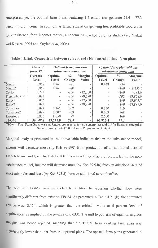
- 50 -
enterprises, yet the optimal farm plans, featuring 4-5 enterprises generate 21.4 - 77.3
percent more income. In addition, as farmers insist on growing less profitable food crops
for subsistence, farm incomes reduce; a conclusion reached by other studies (see Nyikal
and Kosura, 2005 and Kuyiah et al, 2006).
Table 4.2.1(a): Comparison between current and risk-neutral optimal farm plans
Current farm Plan
Optimal farm plan with subsistence constraints
Optimal farm plan without subsistence constraints
C urrentLevel
O ptim alLevel
%C hange
M arginalV alue
O ptim alL evel
%C hange
M arginalV alue
Maize 1 0 .9 6 2 0.761 -21 - 0.438 -54 -
Maize2 0 .9 5 3 0.761 -20 - - -1 0 0 -19,253.6Coffee 0 .2 4 8 - -1 0 0 -12,300 - -1 0 0 -393.6French beans 1 0 .0 1 8 - -1 0 0 -99,590 - -1 0 0 -23,868.6Kales 1 0 .0 2 6 - -1 0 0 -37,950 - -1 0 0 -39,943.7Kales2 0 .0 1 8 - -1 0 0 -38,890 - -1 0 0 -38,895.0Tomatoes 1 0.041 0.165 302 - 0.250 510 -
Tomatoes2 0 .0 1 9 0.007 -63 - 0.203 968 -
Livestock 0 .9 3 0 1.650 77 - 2.500 169 -
TFGM 36,049.2 43,745.8 21.4 - 63,913.4 77.3 -TFGM = Total Farm Gross Margin. Figures are in acres for crop enterprises and LU for livestock enterprise
Source: Survey Data (2009): Linear Programming Output
Marginal analysis presented in the above table indicates that in the subsistence model,
income will decrease most (by Ksh 99,590) from production of an additional acre of
French beans, and least (by Ksh 12,300) from an additional acre of coffee. But in the non
subsistence model, income will decrease most (by Ksh 39,940) from an additional acre of
short rain kales and least (by Ksh 393.5) from an additional acre of coffee.
The optimal TFGMs were subjected to a t-test to ascertain whether they were
significantly different from existing TFGM. As presented in Table 4.2.1(b), the computed
t-value was -2.154, which is greater than the critical t-value at 5 percent level of
significance (as implied by the p-value of 0.033). The null hypothesis of equal farm gross
Margins was hence rejected, meaning that the TFGM from existing farm plan was
Slgnificantly lower than that from the optimal plans. The optimal farm plans generated in
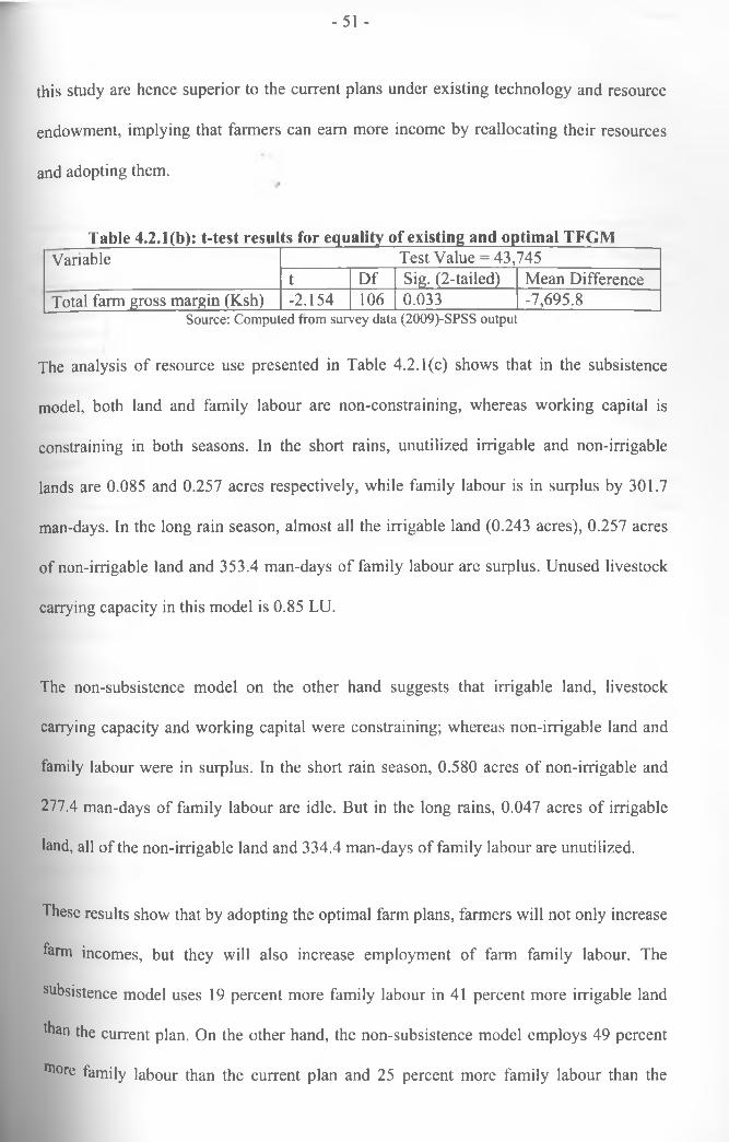
-51 -
this study are hence superior to the current plans under existing technology and resource
endowment, implying that farmers can earn more income by reallocating their resources
and adopting them.
Table 4.2.1(b): t-test results for equality of existing and optimal TFGMVariable Test Value = 43,745
t Df Sig. (2-tailed) Mean DifferenceTotal farm gross margin (Ksh) -2.154 106 0.033 -7,695.8
Source: Computed from survey data (2009)-SPSS output
The analysis of resource use presented in Table 4.2.1(c) shows that in the subsistence
model, both land and family labour are non-constraining, whereas working capital is
constraining in both seasons. In the short rains, unutilized irrigable and non-irrigable
lands are 0.085 and 0.257 acres respectively, while family labour is in surplus by 301.7
man-days. In the long rain season, almost all the irrigable land (0.243 acres), 0.257 acres
of non-irrigable land and 353.4 man-days of family labour are surplus. Unused livestock
carrying capacity in this model is 0.85 LU.
The non-subsistence model on the other hand suggests that irrigable land, livestock
carrying capacity and working capital were constraining; whereas non-irrigable land and
family labour were in surplus. In the short rain season, 0.580 acres of non-irrigable and
277.4 man-days of family labour are idle. But in the long rains, 0.047 acres of irrigable
land, all of the non-irrigable land and 334.4 man-days of family labour are unutilized.
These results show that by adopting the optimal farm plans, farmers will not only increase
farm incomes, but they will also increase employment of farm family labour. The
subsistence model uses 19 percent more family labour in 41 percent more irrigable land
than the current plan. On the other hand, the non-subsistence model employs 49 percent
ITl0re family labour than the current plan and 25 percent more family labour than the
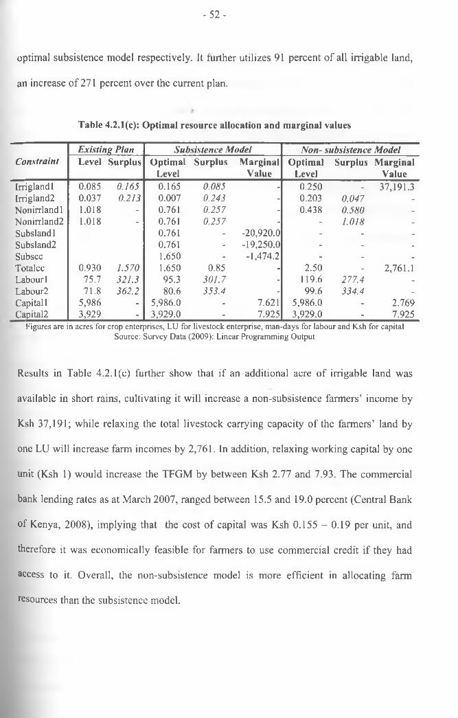
- 5 2 -
optimal subsistence model respectively. It further utilizes 91 percent of all irrigable land,
an increase of 271 percent over the current plan.
Table 4.2.1(c): Optimal resource allocation and marginal values
Existing Plan Subsistence Model Non- subsistence ModelConstraint Level Surplus Optimal Surplus Marginal Optimal Surplus Marginal
Level Value Level ValueIrriglandl 0.085 0.165 0.165 0.085 - 0.250 - 37,191.3Irrigland2 0.037 0.213 0.007 0.243 - 0.203 0.047 -
Nonirrlandl 1.018 - 0.761 0.257 - 0.438 0.580 -
Nonirrland2 1.018 - 0.761 0.257 - - 1.018 -
Subslandl 0.761 - -20,920.0 - - -
Subsland2 0.761 - -19,250.0 - - -
Subscc 1.650 - -1,474.2 - - -
Totalcc 0.930 1.570 1.650 0.85 - 2.50 - 2,761.1Labour 1 75.7 321.3 95.3 301.7 - 119.6 277.4 -
Labour2 71.8 362.2 80.6 353.4 - 99.6 334.4 -
Capital 1 5,986 - 5,986.0 - 7.621 5,986.0 - 2.769Capital2 3,929 - 3,929.0 - 7.925 3,929.0 - 7.925
Figures are in acres for crop enterprises, LU for livestock enterprise, man-days for labour and Ksh for capital Source: Survey Data (2009): Linear Programming Output
Results in Table 4.2.1(c) further show that if an additional acre of irrigable land was
available in short rains, cultivating it will increase a non-subsistence farmers’ income by
Ksh 37,191; while relaxing the total livestock carrying capacity of the farmers’ land by
one LU will increase farm incomes by 2,761. In addition, relaxing working capital by one
unit (Ksh 1) would increase the TFGM by between Ksh 2.77 and 7.93. The commercial
bank lending rates as at March 2007, ranged between 15.5 and 19.0 percent (Central Bank
of Kenya, 2008), implying that the cost of capital was Ksh 0.155-0.19 per unit, and
therefore it was economically feasible for farmers to use commercial credit if they had
access to it. Overall, the non-subsistence model is more efficient in allocating farm
resources than the subsistence model.
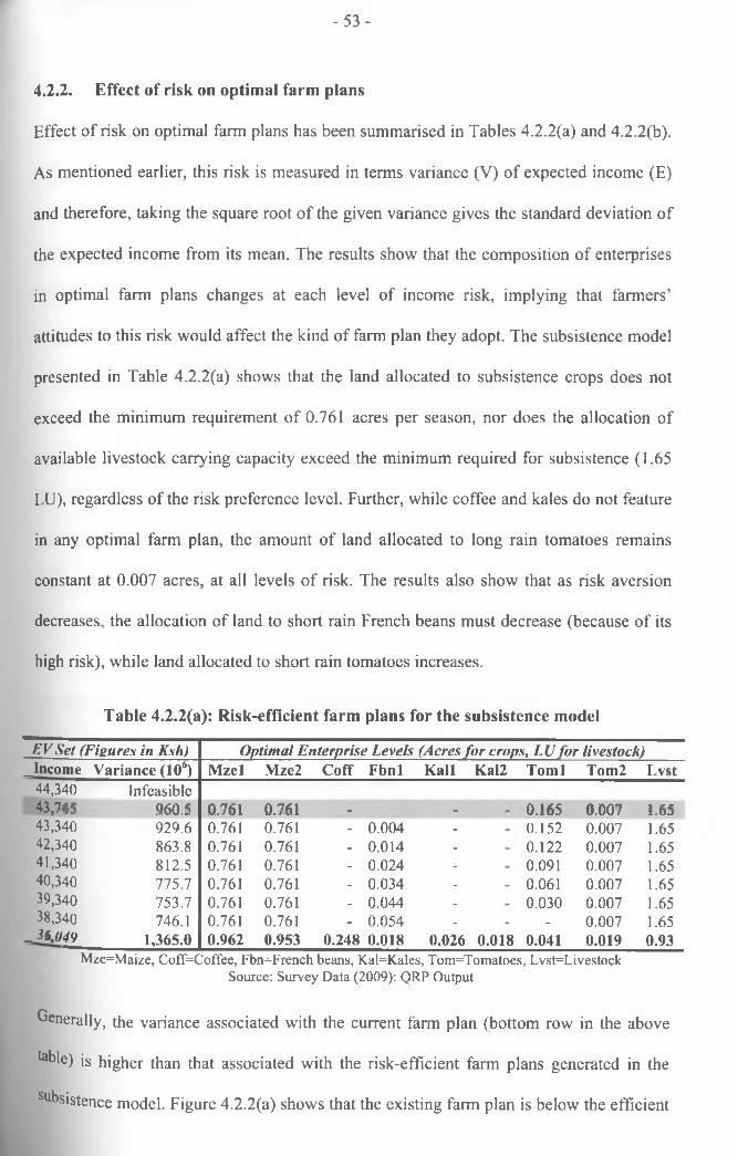
- 5 3 -
4.2.2. Effect of risk on optimal farm plans
Effect of risk on optimal farm plans has been summarised in Tables 4.2.2(a) and 4.2.2(b).
As mentioned earlier, this risk is measured in terms variance (V) of expected income (E)
and therefore, taking the square root of the given variance gives the standard deviation of
the expected income from its mean. The results show that the composition of enterprises
in optimal farm plans changes at each level of income risk, implying that farmers’
attitudes to this risk would affect the kind of farm plan they adopt. The subsistence model
presented in Table 4.2.2(a) shows that the land allocated to subsistence crops does not
exceed the minimum requirement of 0.761 acres per season, nor does the allocation of
available livestock carrying capacity exceed the minimum required for subsistence (1.65
LU), regardless of the risk preference level. Further, while coffee and kales do not feature
in any optimal farm plan, the amount of land allocated to long rain tomatoes remains
constant at 0.007 acres, at all levels of risk. The results also show that as risk aversion
decreases, the allocation of land to short rain French beans must decrease (because of its
high risk), while land allocated to short rain tomatoes increases.
Table 4.2.2(a): Risk-efficient farm plans for the subsistence model
EV Set (Fisures in Ksh) Optimal Enterprise Levels (Acres for crops, LUfor livestock)_Income Variance (106) Mzel Mze2 Coff Fbnl Kail Kal2 Toml Tom2 L vst
44,340 Infeasible43,745 960.5 0.761 0.761 - - 0.165 0.007 1.6543,340 929.6 0.761 0.761 - 0.004 - 0.152 0.007 1.6542,340 863.8 0.761 0.761 - 0.014 - 0.122 0.007 1.6541,340 812.5 0.761 0.761 - 0.024 - 0.091 0.007 1.6540,340 775.7 0.761 0.761 - 0.034 - 0.061 0.007 1.6539,340 753.7 0.761 0.761 - 0.044 - 0.030 0.007 1.6538,340 746.1 0.761 0.761 - 0.054 - - 0.007 1.65
_ 36,049 1,365.0 0.962 0.953 0.248 0.018 0.026 0.018 0.041 0.019 0.93Mze=Maize, Coff=Coffee, Fbn=French beans, Kal=Kales, Tom=Tomatoes, Lvst=Livestock
Source: Survey Data (2009): QRP Output
Generally, the variance associated with the current farm plan (bottom row in the above
^ble) is higher than that associated with the risk-efficient farm plans generated in the
Subsistence model. Figure 4.2.2(a) shows that the existing farm plan is below the efficient
- 5 4 -
EV frontier. The implication is that the current farm plan is highly risky, yet farmers
diversify with the aim of reducing risk. The most risk-averse farmer can optimize risk by
dropping coffee, kales and short rain tomatoes from the current farm plans, growing 0.761
acres of maize intercrop in both seasons, 0.054 acres of French beans in short rains and
0.007 acres of tomatoes in long rains, and keeping 1.65 LU. This farm plan will earn the
farmer an expected income of Ksh 38,340, which has a variance of 746 million (equal to a
standard deviation of KSh 27,315).
On the other hand, the subsistence-oriented farmer with least risk-aversion can earn an
expected income of Ksh 43,745, with a variance of 960.5 million (standard deviation of
KSh 30,992), by growing 0.761 acres of maize intercrop in both short and long rain
seasons; 0.165 acres of tomatoes in the short rains and 0.007 acres of tomatoes in long
rain season; and keeping 1.65 LU. This farm plan can be recommended for adoption
under current level of resource availability because the variance associated with it is 30
percent less than that of the existing farm plan, yet it earns farmers 21 percent more
income, utilises 41 percent more irrigable land and increases employment of family
labour by 19 percent. Detailed information on resource requirement/allocation for this
model can be obtained from Appendix 6 (plan VII).
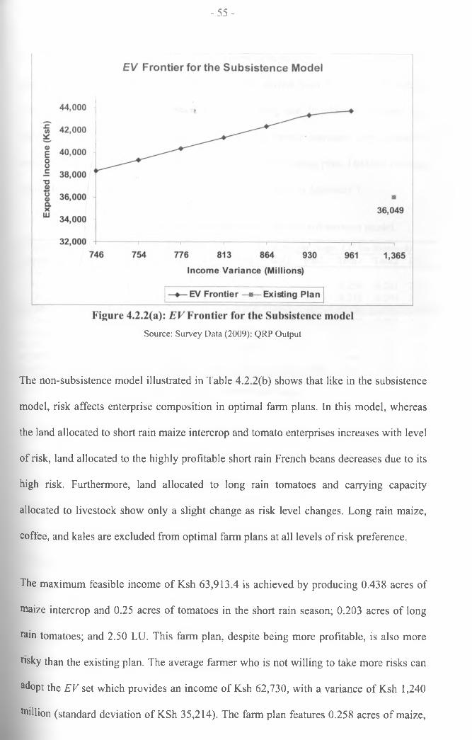
- 55 -
Source: Survey Data (2009): QRP Output
The non-subsistence model illustrated in Table 4.2.2(b) shows that like in the subsistence
model, risk affects enterprise composition in optimal farm plans. In this model, whereas
the land allocated to short rain maize intercrop and tomato enterprises increases with level
of risk, land allocated to the highly profitable short rain French beans decreases due to its
high risk. Furthermore, land allocated to long rain tomatoes and carrying capacity
allocated to livestock show only a slight change as risk level changes. Long rain maize,
coffee, and kales are excluded from optimal farm plans at all levels of risk preference.
The maximum feasible income of Ksh 63,913.4 is achieved by producing 0.438 acres of
maize intercrop and 0.25 acres of tomatoes in the short rain season; 0.203 acres of long
min tomatoes; and 2.50 LU. This farm plan, despite being more profitable, is also more
nsky than the existing plan. The average farmer who is not willing to take more risks can
adopt the EV set which provides an income of Ksh 62,730, with a variance of Ksh 1,240
million (standard deviation of KSh 35,214). The farm plan features 0.258 acres of maize,
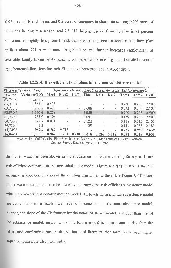
- 56 -
0.05 acres of French beans and 0.2 acres of tomatoes in short rain season; 0.203 acres of
tomatoes in long rain season; and 2.5 LU. Income earned from the plan is 73 percent
more and is slightly less prone to risk-than the existing one. In addition, the farm plan
utilises about 271 percent more irrigable land and further increases employment of
available family labour by 47 percent, compared to the existing plan. Detailed resource
requirements/allocations for each EV set have been provided in Appendix 7.
Table 4.2.2(b): Risk-efficient farm plans for the non-subsistence model
EV Set (Figures in Ksh) Optimal Enterprise Levels (Acres for crops, LU for livestock)Income Variance(106) Mzel Mze2 Coff Fbnl Kail Kal2 Toml Tom2 Lvst63,730.063,913.4
Infeasible1,863.1 0.438 0.250 0.203 2.500
63,730.0 1,760.8 0.410 - - 0.008 - - 0.242 0.203 2.50062,730.0 1,240.4 0.258 - - 0.050 - - 0.200 0.203 2.50061,730.0 783.0 0.106 - - 0.091 - - 0.159 0.203 2.50060,730.0 379.8 0.014 - - 0.122 - - 0.128 0.212 2.40659,730.0 1.2 - - - 0.139 - - 0.111 0.235 2.18343,745.0 960.4 0.761 0.761 - - - - 0.165 0.007 1.65036,049.2 1,365.0 0.962 0.953 0.248 0.018 0.026 0.018 0.041 0.019 0.930
Mze=Maize, Coff-Coffee, Fbn-French beans, Kal=K.ales, Tom=Tomatoes, Lvst=Livestock Source: Survey Data (2009): QRP Output
Similar to what has been shown in the subsistence model, the existing farm plan is not
risk-efficient compared to the non-subsistence model. Figure 4.2.2(b) illustrates that the
income-variance combination of the existing plan is below the risk-efficient EV frontier.
The same conclusion can also be made by comparing the risk-efficient subsistence model
with the risk-efficient non-subsistence model. All levels of risk in the subsistence model
are associated with a much lower level of income than in the non-subsistence model.
Further, the slope of the EV frontier for the non-subsistence model is steeper than that of
the subsistence model, implying that the former model is more prone to risk than the
latter, and confirming earlier observations and literature that farm plans with higher
expected returns are also more risky.
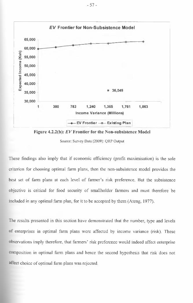
- 57 -
EV Frontier for Non-Subsistence Model
.C</>*<DEoocT3<1)|Q.XUJ
65.000
60.000
55.000
50.000
45.000
40.000
35.000
30.000380
• 36,049
783 1,240 1,365 1,761Income Variance (Millions)
EV Frontier — Existing Plan
1,863
Figure 4.2.2(b): EV Frontier for the Non-subsistence Model
Source: Survey Data (2009): QRP Output
These findings also imply that if economic efficiency (profit maximisation) is the sole
criterion for choosing optimal farm plans, then the non-subsistence model provides the
best set of farm plans at each level of farmer’s risk preference. But the subsistence
objective is critical for food security of smallholder farmers and must therefore be
included in any optimal farm plan, for it to be accepted by them (Ateng, 1977).
The results presented in this section have demonstrated that the number, type and levels
of enterprises in optimal farm plans were affected by income variance (risk). These
observations imply therefore, that farmers’ risk preference would indeed affect enterprise
composition in optimal farm plans and hence the second hypothesis that risk does not
affect choice of optimal farm plans was rejected.
- 5 8 -
4.2.3. Mitigating risk: relaxing the working capital constraint
The results presented in sections 4.2.1 and 4.2.2 have shown that the subsistence model
provides optimal farm plans with lower expected income that the non-subsistence models.
However, subsistence model is deemed more realistic to farmers’ conditions and hence
more likely to be accepted by farmers. In view of this, it became necessary to subject the
subsistence model to some sensitivity analysis12 to assess possibility of lowering income
risk associated with this model.
In this study, varying the maximum available working capital was preferred, because
working capital was the only constraining resource in optimal farm plans for the
subsistence model, as illustrated in Table 4.2.1(b). In addition, farmers in the study area
had in the focus group discussion identified working capital as their most limiting
farming constraint13. It has also been established that while farmers in Machakos District
invest low levels of capital and land as a strategy for mitigating farming risks associated
with erratic rainfall, such a strategy makes the farmers not to exploit opportunities
presented by good seasons (Rao and Okwach, 2005). Investigating the effect of easing
working capital on optimal farm plans would therefore provide guidelines on how the
farmers can invest the additional capital to minimize farm income risk. EV sets were
generated and analysed under unconstrained capital in season 1; unconstrained capital in
season 2; and unconstrained capital in both seasons14. The results of each capital
availability regime were compared with those in which capital was constrained in both
seasons (baseline plans), and the existing plans. The results have been presented below.
12 Sensitivity analysis evaluates how a model’s results will be affected by changes in input values or assumptions (Pasky et al, 2003), and it should concern itself only with changes in inputs (or assumptions) that will lead to different decisions (Frey, 2002). To do this, Panned (1997) suggests that one could vary the contribution o f an activity to the objective; the objective function; a constraint limit; the number of constraints; the number o f activities; or technical parameters; and observe the changes for instance in values of objective function or decision variables.^Some studies also report that most farmers lack access to capital (see for example, Place et al, 2006).
Seasonl refers to short rains season, while season2 refers to long rains season.
- 5 9 -
(a) Risk-efficient subsistence model with unconstrained capital in season 1
Results of the sensitivity analysis show that it would require an additional Ksh 731 (7.3f
percent) to completely relax the capital constraints in the short rains season. This would
result in risk-efficient farm plans that earn the farmer maximum expected returns of Ksh
49,134. The total expected returns earned exceed those provided by the baseline plans by
Ksh 5,389 (12.3 percent), but also increase income variance by 29 percent. However, the
risk level associated with this farm plan is still 10 percent less, while the income earned
would be 36 percent more, compared to the existing plan. This means that by relaxing
working capital constraints, income risks would reduce and farmers would improve their
efficiency, as shown in the EV frontier map in Figure 4.2.3.
As shown in Table 4.2.3(a), the land allocated to subsistence crops does not exceed the
minimum requirement. French beans features in lower risk farm plans but is excluded in
the most profitable farm plan. The best feasible farm plan features 0.761 acres of maize
intercrop in both seasons; 0.25 acres of tomatoes in season 1; and 1.72 LU. This farm
plan utilises about 111 percent more irrigable land than the current plan. It also increases
returns to working capital from KSh 3.6 to KSh 4.6 per shilling invested, representing a
27 percent increase, and increases employment of family labour by 27 percent. Assuming
that the farmers’ risk preference remains at the level depicted in the existing farm plan,
farmers with access to adequate capital in short rains season only can be advised to adopt
this farm plan. Detailed resource requirements and allocations for each EV set are
provided in Appendix 8.
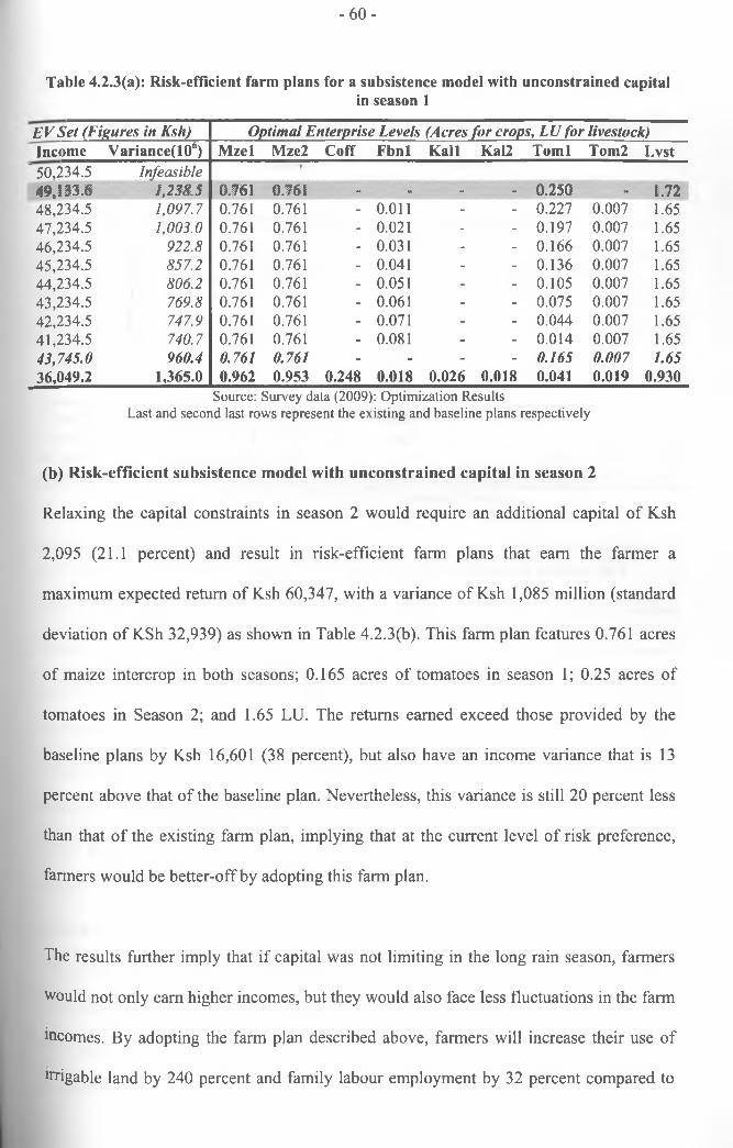
- 60 -
Table 4.2.3(a): Risk-efficient farm plans for a subsistence model with unconstrained capitalin season 1
EVSet (Figures in Ksh) Optimal Enterprise Levels (Acres for crops, LU for livestock)Income Variance(106) Mzel Mze2 Coff Fbnl Kail Kal2 Toml Tom2 Lvst
" 50,234.5 Infeasible I
49,133.6 1,238.5 0.761 0.761 - m - •• 0.250 - 1.7248,234.5 1,097.7 0.761 0.761 - 0.011 - - 0.227 0.007 1.6547,234.5 1,003.0 0.761 0.761 - 0.021 - - 0.197 0.007 1.6546,234.5 922.8 0.761 0.761 - 0.031 - - 0.166 0.007 1.6545,234.5 857.2 0.761 0.761 - 0.041 - - 0.136 0.007 1.6544,234.5 806.2 0.761 0.761 - 0.051 - - 0.105 0.007 1.6543,234.5 769.8 0.761 0.761 - 0.061 - - 0.075 0.007 1.6542,234.5 747.9 0.761 0.761 - 0.071 - - 0.044 0.007 1.6541,234.5 740.7 0.761 0.761 - 0.081 - - 0.014 0.007 1.6543,745.0 960.4 0.761 0.761 - - - - 0.165 0.007 1.6536,049.2 1,365.0 0.962 0.953 0.248 0.018 0.026 0.018 0.041 0.019 0.930
Source: Survey data (2009): Optimization Results Last and second last rows represent the existing and baseline plans respectively
(b) Risk-efficient subsistence model with unconstrained capital in season 2
Relaxing the capital constraints in season 2 would require an additional capital of Ksh
2,095 (21.1 percent) and result in risk-efficient farm plans that earn the farmer a
maximum expected return of Ksh 60,347, with a variance of Ksh 1,085 million (standard
deviation of KSh 32,939) as shown in Table 4.2.3(b). This farm plan features 0.761 acres
of maize intercrop in both seasons; 0.165 acres of tomatoes in season 1; 0.25 acres of
tomatoes in Season 2; and 1.65 LU. The returns earned exceed those provided by the
baseline plans by Ksh 16,601 (38 percent), but also have an income variance that is 13
percent above that of the baseline plan. Nevertheless, this variance is still 20 percent less
than that of the existing farm plan, implying that at the current level of risk preference,
farmers would be better-off by adopting this farm plan.
The results further imply that if capital was not limiting in the long rain season, farmers
would not only earn higher incomes, but they would also face less fluctuations in the farm
incomes. By adopting the farm plan described above, farmers will increase their use of
urigable land by 240 percent and family labour employment by 32 percent compared to
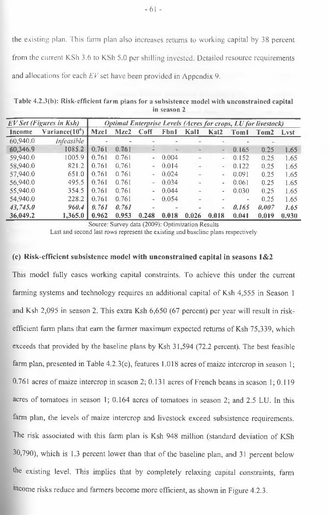
-61 -
the existing plan. This farm plan also increases returns to working capital by 38 percent
from the current KSh 3.6 to KSh 5.0 per shilling invested. Detailed resource requirements
and allocations for each EV set have been provided in Appendix 9.
Table 4.2.3(b): Risk-efficient farm plans for a subsistence model with unconstrained capitalin season 2
EV Set (Figures in Ksh) Optimal Enterprise Levels (Acres for crops, LU for livestock)Income Variance! 106) Mzel Mze2 Coff Fbnl Kail Kal2 Toml Tom2 Lvst60,940.0 Infeasible - - - - - - -
60,346.9 1085.2 0.761 0.761 ■ Wk £ «* 0.165 0.25 1.6559,940.0 1005.9 0.761 0.761 - 0.004 - 0.152 0.25 1.6558,940.0 821.2 0.761 0.761 - 0.014 - 0.122 0.25 1.6557,940.0 651.0 0.761 0.761 - 0.024 - 0.091 0.25 1.6556,940.0 495.5 0.761 0.761 - 0.034 - 0.061 0.25 1.6555,940.0 354.5 0.761 0.761 - 0.044 - 0.030 0.25 1.6554,940.0 228.2 0.761 0.761 - 0.054 - - 0.25 1.6543,745.0 960.4 0.761 0.761 - - - 0.165 0.007 1.6536,049.2 1,365.0 0.962 0.953 0.248 0.018 0.026 0.018 0.041 0.019 0.930
Source: Survey data (2009): Optimization Results Last and second last rows represent the existing and baseline plans respectively
(c) Risk-efficient subsistence model with unconstrained capital in seasons 1&2
This model fully eases working capital constraints. To achieve this under the current
farming systems and technology requires an additional capital of Ksh 4,555 in Season 1
and Ksh 2,095 in season 2. This extra Ksh 6,650 (67 percent) per year will result in risk-
efficient farm plans that earn the farmer maximum expected returns of Ksh 75,339, which
exceeds that provided by the baseline plans by Ksh 31,594 (72.2 percent). The best feasible
farm plan, presented in Table 4.2.3(c), features 1.018 acres of maize intercrop in season 1;
0.761 acres of maize intercrop in season 2; 0.131 acres of French beans in season 1; 0.119
acres of tomatoes in season 1; 0.164 acres of tomatoes in season 2; and 2.5 LU. In this
farm plan, the levels of maize intercrop and livestock exceed subsistence requirements.
The risk associated with this farm plan is Ksh 948 million (standard deviation of KSh
30,790), which is 1.3 percent lower than that of the baseline plan, and 31 percent below
the existing level. This implies that by completely relaxing capital constraints, farm
mcome risks reduce and farmers become more efficient, as shown in Figure 4.2.3.
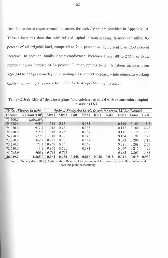
- 6 2 -
Detailed resource requirements/allocations for each EV set are provided in Appendix 10.
These allocations show that with relaxed capital in both seasons, farmers can utilise 83
percent of all irrigable land, compared to 24.4 percent in the current plan (239 percent
increase). In addition, family labour employment increases from 148 to 272 man days,
representing an increase of 84 percent. Further, returns to family labour increase from
KSh 244 to 277 per man day, representing a 14 percent increase, while returns to working
capital increase by 25 percent from KSh 3.6 to 4.5 per Shilling invested.
Table 4.2.3(c): Risk-efficient farm plans for a subsistence model with unconstrained capitalin seasons 1&2
EV Set (Figures in Ksh) Optimal Enterprise Levels (Acres for crops, LU foi livestock)Income Variance(106) Mzel Mze2 Coff Fbnl Kali Kal2 Toml Tom2 Lvst75,500.0 Infeasible75,338.8 948.0 1.018 0.761 0.131 0.119 0.164 2.575,250.0 912.4 1.018 0.761 0.133 0.117 0.166 2.4874,750.0 716.9 1.018 0.761 0.139 0.111 0.178 2.3674,250.0 529.5 1.018 0.761 0.146 0.104 0.191 2.2373,750.0 349.2 0.997 0.761 0.157 0.093 0.200 2.1573,250.0 173.1 0.969 0.761 0.169 0.081 0.208 2.0772,750.0 1.1 0.940 0.761 0.181 0.069 0.215 1.9943,745.0 960.4 0.761 0.761 - - - - 0.165 0.007 1.6536,049.2 1,365.0 0.962 0.953 0.248 0.018 0.026 0.018 0.041 0.019 0.930
Source: Survey data (2009): Optimization Results. Last and second last rows represent the existing andbaseline plans respectively
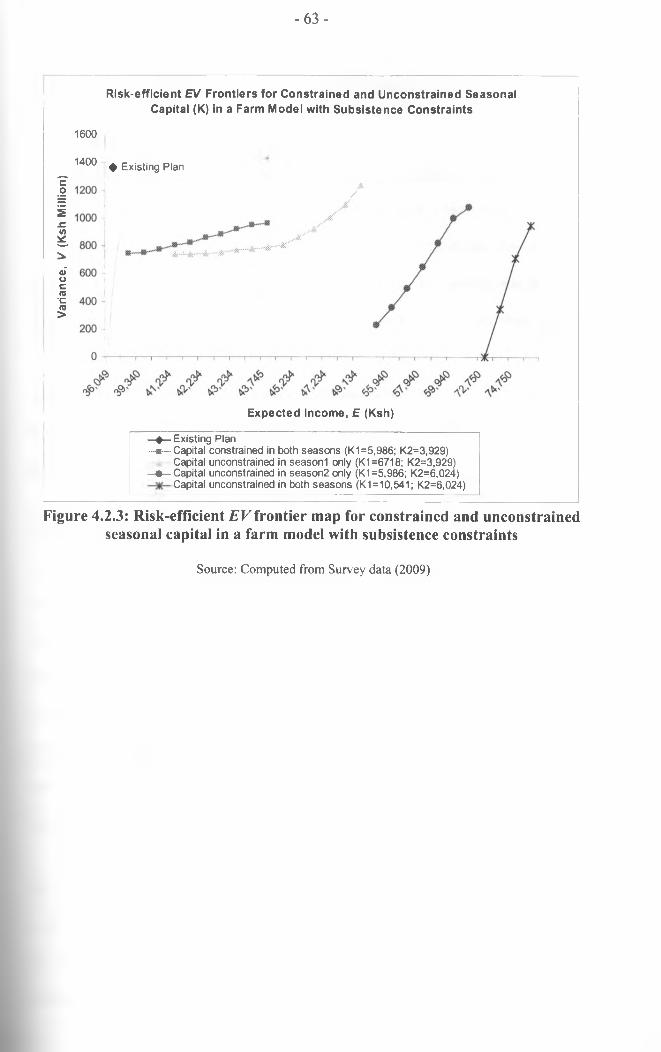
Varia
nce,
V (
Ksh
Mill
ion)
- 6 3 -
Risk-efficient E V Frontiers for Constrained and Unconstrained Seasonal Capital (K) in a Farm Model with Subsistence Constraints
1600
1400 ♦ Existing Plan
Expected Income, E (Ksh)
—# — Existing Plan—«s—• Capital constrained in both seasons (K1 =5,986; K2=3,929)
Capital unconstrained in seasonl only (K1 =6718; K2=3,929)—• — Capital unconstrained in season2 only (K1 =5,986; K2=6,024)
Capital unconstrained in both seasons (K1=10,541; K2=6,024)
Figure 4.2.3: Risk-efficient EV frontier map for constrained and unconstrained seasonal capital in a farm model with subsistence constraints
Source: Computed from Survey data (2009)
- 6 4 -
Chapter 5: Summary, Conclusions and Recommendations
5.1 Summary and Conclusions
This study assessed the effect of farm income risks on production decisions in Kauti
Irrigation Scheme in the highlands of Machakos District, with a view to identifying farm
plans that earn farmers higher incomes at existing or lower levels of risk. Two hypotheses
were tested: one, that existing farm plans in the study area are optimal; and the second,
that risk preference does not affect choice of optimal farm plans in the study area. The
study used crop and livestock production and marketing data covering 2007/08 short rains
and 2008 long rains seasons. The survey was conducted in March 2009 through a farm
household survey involving 113 households. The data were analysed using linear and
quadratic risk programming techniques.
The risk-neutral farm plans produced by the linear program show that with subsistence
constraints, the farmer would earn an expected total farm gross margin (TFGM) of Ksh
43,746 compared to Ksh 36,049 from the existing farm plan, representing a 21.4 percent
increase. On the other hand, without subsistence constraints, the farmer would earn an
expected TFGM of Ksh 63,913, which is 77.3 percent above the existing level, and 46.1
percent above the income from optimal plan with subsistence restrictions. In both models,
coffee, kales and French beans are excluded from the optimal plans. The resultant optimal
farm plans comprise only 4 enterprises (5 if subsistence constraints are imposed) as
opposed to 9 in a typical farm plan in the irrigation scheme.
The differences in TFGM between optimal and existing farm plans were statistically
significant; hence the null hypothesis of equal TFGM was rejected. The implication is
that the current farm plan operated in the study area is sub-optimal, and farmers can
therefore improve their farm incomes under the current production technology by simply
- 6 5 -
reallocating their resources to adopt optimal farm plans. In addition, as farmers produce
for subsistence, they earn less income, implying that a non-subsistence farm model would
utilize farm resources more efficiently than a subsistence one. However, the subsistence
objective is critical for the smallholder farmers’ food security; hence it would be more
realistic for farmers to adopt farm plans that impose minimum subsistence requirements.
Alternatively, if farmers were to increase their productivity, the subsistence needs would
be easily achieved and thus be less of a challenge to commercialization or adoption of
optimal plans as recommended here.
The analysis of resource allocation shows that whereas land, labour and livestock
carrying capacities were underutilized in the risk-neutral farm plans, working capital was
constraining. The Marginal Value Product (MVP) of capital in the optimal farm plans was
at least 2.77, whereas the prevailing cost of bank credit was at most 0.19 per unit, during
the period under study. This implies that it was economically feasible for farmers to use
bank credit if they had access to it. Further, the results show that the optimal farm plans
increase employment of farm family labour by upto 49 percent and utilization of irrigable
land by up to 271 percent, over the current plan.
Results of the quadratic risk programming (QRP) under both the subsistence and non
subsistence models suggest different levels of land allocation to French beans and
tomatoes in short rains season, at each level of income risk. Generally, as risk aversion
decreases, farmers should allocate less land to French beans, and more land to tomatoes,
in order to be risk-efficient. These results show that farm income risk affects the
composition of enterprises in the optimal farm plan and hence farmers’ production
decisions and incomes. The results further show that the EV combination of existing farm
Plan falls below the risk-efficient frontiers for both subsistence and non-subsistence
- 6 6 -
models, implying that although the existing farm plan is highly diversified, it is not risk-
efficient. The risk model without subsistence constraint was also found to be more
profitable and risky than the risk model with subsistence constraints. However, the
subsistence plan is more likely to be adopted by farmers since it promotes household food
self-sufficiency.
Sensitivity analysis indicates that relaxing capital constraints would result in risk-efficient
farm plans that increase expected income by up to 109 percent compared to existing farm
plan, and by up to 72 percent compared to optimal farm plans under constrained capital.
Further, the farm plans reduce income risk by up to 31 percent and increase utilization of
irrigable land by 240 percent; family labour employment by 84 percent; returns to family
labour by 14 percent; and returns to working capital by 25 percent. The greatest impact
would come from relaxing capital in both short and long rains seasons, implying that if
farmers had access to adequate capital throughout the year, they would bring most of the
idle irrigable land into production and adopt farm plans that reduce risks and earn them
more incomes. Alternatively, if strategies were put in place to minimize fluctuations in
farm incomes, then farmers would invest more capital in farming and adopt farm plans
that earn them more incomes.
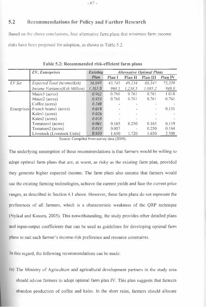
- 6 7 -
5.2 Recommendations for Policy and Further Research
Based on the above conclusions, four alternative farm plans that minimize farm income
risks have been proposed for adoption, as shown in Table 5.2.
Table 5.2: Recommended risk-efficient farm plans
EV, Enterprises Existing_ Alternative Optimal PlansPlan Plan 1 Plan II Plan III Plan IV
EVSet Expected Total Income(Ksh) 36,049 43,745 49,134 60,347 75,339Income Variance(Ksh M illion ) 1,365.0 960.5 1,238.5 1,085.2 948.0Maize 1 (acres) 0.962 0.761 0.761 0.761 1.018Maize2 (acres) 0.953 0.761 0.761 0.761 0.761Coffee (acres) 0.248 - - - -
Enterprises French beans 1 (acres) 0.018 - - - 0.131Kales 1 (acres) 0.026 - - - -Kales2 (acres) 0.018 - - - -
Tomatoes 1 (acres) 0.041 0.165 0.250 0.165 0.119Tomatoes2 (acres) 0.019 0.007 - 0.250 0.164Livestock (Livestock Units) 0.930 1.650 1.720 1.650 2.500
Source: Compiled from survey data (2009).
The underlying assumption of these recommendations is that farmers would be willing to
adopt optimal farm plans that are, at worst, as risky as the existing farm plan, provided
they generate higher expected income. The farm plans also assume that farmers would
use the existing farming technologies, achieve the current yields and face the current price
ranges, as described in Section 4.1 above. However, these farm plans do not represent the
preferences of all farmers, which is a characteristic weakness of the QRP technique
(Nyikal and Kosura, 2005). This notwithstanding, the study provides other detailed plans
and input-output coefficients that can be used as guidelines for developing optimal farm
plans to suit each farmer’s income-risk preference and resource constraints.
In this regard, the following recommendations can be made:
(a) The Ministry of Agriculture and agricultural development partners in the study area
should advise farmers to adopt optimal farm plan IV. This plan suggests that farmers
abandon production of coffee and kales. In the short rains, farmers should allocate
- 68 -
1.018 acres to maize intercrop, 0.131 acres to French beans, and 0.119 acres to
tomatoes; while in the long rains, they should allocate 0.761 acres to maize intercrop
and 0.164 acres for tomatoes. In addition, the farmers should keep an average of 2.5
livestock units (equivalent to 2 improved dairy cows or 1 improved dairy cow + 5
mature goats) throughout the year.
This farm plan would earn farmers a total expected income of Ksh 75,339 annually,
which is more than double the current income. The income risk (variance) associated
with this farm plan is Ksh 948 million (standard deviation of KSh 30,790 and is 31
percent less than that associated with the existing farm plan. Furthermore, this farm
plan increases employment of family labour from the current 148 to 272 man days,
representing 84 percent increase. Returns to family labour also increase from the
existing Ksh 244 to Ksh 277 per man-day, an improvement of about 13 percent.
It should be noted, however, that this plan requires a working capital of Ksh 16,565,
which exceeds the current capital availability by Ksh 6,650 (67 percent). This calls for
increased access to working capital by farmers. Although the government (in
partnership with some donors and private sector players) has set up some farm input
financing programmes, most of them are sector-specific (for instance, Kilimo
Biashara for cereals and Smallholder Horticultural Marketing Programme, SHoMaP,
for horticultural crops), despite the government’s call for diversification of
agricultural activities by smallholder farmers. Furthermore, in the study area, most
farmers have not accessed credit through such programmes15. There is need to assess
the efficacy of these programmes, with the aim of developing a financing strategy that
would allow many farmers to apply at once for a ‘comprehensive’ credit that would
cater for working capital requirements of a diversified, risk-efficient farm plan.
Information source: Ministry o f Agriculture extension staff and farmers in the study area.
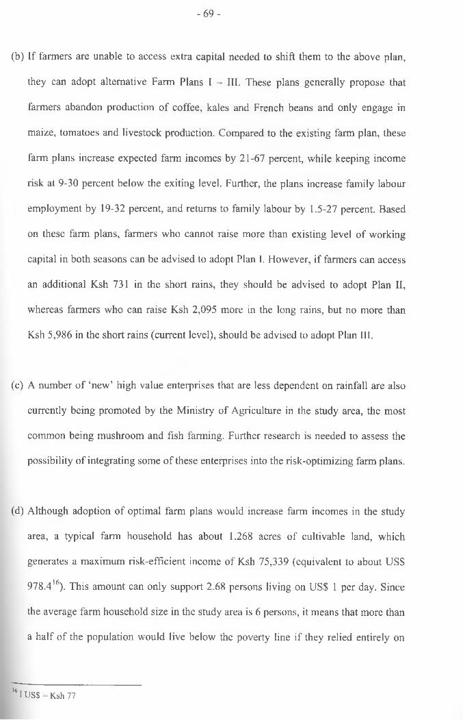
- 6 9 -
(b) If farmers are unable to access extra capital needed to shift them to the above plan,
they can adopt alternative Farm Plans I - III. These plans generally propose that
farmers abandon production of coffee, kales and French beans and only engage in
maize, tomatoes and livestock production. Compared to the existing farm plan, these
farm plans increase expected farm incomes by 21 -67 percent, while keeping income
risk at 9-30 percent below the exiting level. Further, the plans increase family labour
employment by 19-32 percent, and returns to family labour by 1.5-27 percent. Based
on these farm plans, farmers who cannot raise more than existing level of working
capital in both seasons can be advised to adopt Plan I. However, if farmers can access
an additional Ksh 731 in the short rains, they should be advised to adopt Plan II,
whereas farmers who can raise Ksh 2,095 more in the long rains, but no more than
Ksh 5,986 in the short rains (current level), should be advised to adopt Plan III.
(c) A number of ‘new’ high value enterprises that are less dependent on rainfall are also
currently being promoted by the Ministry of Agriculture in the study area, the most
common being mushroom and fish farming. Further research is needed to assess the
possibility of integrating some of these enterprises into the risk-optimizing farm plans.
(d) Although adoption of optimal farm plans would increase farm incomes in the study
area, a typical farm household has about 1.268 acres of cultivable land, which
generates a maximum risk-efficient income of Ksh 75,339 (equivalent to about US$
978.4 16). This amount can only support 2.68 persons living on US$ 1 per day. Since
the average farm household size in the study area is 6 persons, it means that more than
a half of the population would live below the poverty line if they relied entirely on
161 USS = Ksh 77
- 7 0 -
• 1 7 • i ,farming . With increasing population, land subdivision is likely to further worsen the
situation. Furthermore, even the most efficient farm plan would employ only 272 out
of 831 man-days (33 percent) of family labour available annually. In light of this, the
government, in collaboration with development partners, should develop and support
more strategies that increase employment opportunities in the off-farm sector.
17The current poverty in the study area level is estimated at 65 percent.
- 7 1 -
References
Adams, R.M., D.J. Menkhaus and B.A. Woolery. (1980). Alternative Parameter Specification in E, V Analysis: Implications for Farm Level Decision Making. Western Jou rna l o f A g ricu ltu ra l Economics (1980): 13-20.
Adesiyan, O.I., W.A. Samusi and B.A. Salako. (2007). Optimum Enterprise Combination in Maize Farm in Orire Local Govemmaent Area of Oyo State, Nigeria. Pakistan Journa l o f Socia l Sciences 4(2): 256-278.
Alford, A.R., G.R. Griffith, and O. Cacho. (2004). A N orthern Tablelands Whole-Farm L in e a r P rogram fo r Econom ic Evalua tion o f New Technologies a t the Farm Level. Economic Research Report No. 13. NSW Agriculture, Armidale.
Ateng, B.A. (1977). Linear Programming: An Application to the Identification of the Best Existing Farming Strategy for Peasant Farmers in Kenya. Unpublished MA Thesis, University of Nairobi.
Babatunde, R.O., E.O. Olorunsanya, J.S. Orebiyi and A. Falola. (2007). Optimal Farm Plan in Potato Cropping Systems: The Case of Offa and Oyun Local Government Areas of Kwara State, North-Central Nigeria. A g ricu ltu ra l Journa l 2(2): 285-289.
Barkley, A., and H.H. Peterson. (2008). [Online], Wheat Variety Selection: An Application of Portfolio Theory to Improve Returns. Proceedings o f the NCCC-134 Conference on A pp lied Commodity P rice Analysis, Forecasting, and M arket Risk Management H e ld at St. Louis, M issouri on A p r il 21-22, 2008. Available from:http://www.farmdoc.uiuc.edu/ncccl34. Date Accessed: 3rd February 2009.
Bartlett, J.E., J.W. Kotrlik and C.C. Higgins. (2001). Organizational research: Determining appropriate sample size in survey research. In form ation Technology, Learning, and Perform ance Jo u rna l 19(1): 43-50.
Bhende, M.J. and J.V. Venkataram. (1994). The Impact of Diversification on Household Income and Risk: A Whole Farm Modelling Approach. A g ricu ltu ra l Systems 44(3): 301-312.
Bhowmick, B.C. (2005). Risk in Agribusiness. Lecture delivered on 12th May 2005 in the training programme arranged under Agriclinic and Agri-business Centre Programmes sponsored by MANAGE, Hyderabad; NABARD and SFAC and organized by the Directorate of Extension Education, Assam Agricultural University, Jorhat-13.
Central Bank of Kenya. (2008). Survey on Bank Charges and Lending Rates. Nairobi Kenya: the Central Bank of Kenya.
Crisostomo, M.F. and A.M. Featherstone. (1990). Portfolio Analysis of Returns to Farm Equity and Assets. N orth C entra l Jou rna l o f A g ricu ltu ra l Economics 12(1): 9-21
Dantzig, G.B. (1998). L in ea r Program m ing and Extensions. 11th Edition. Princeton University Press.
- 7 2 -
De Groote, H., C.Doss, S.D. Lyimo and W. Mwangi. (2002). Adoption of Maize Technologies in East Africa - What Happened to Africa’s Emerging Maize Revolution? Paper p repa red f o r the FASID Forum V, on " Green Revolution in Asia and its T ransferability to A fr ica ” he ld in Tokyo, Japan on December 8-10, 2002.
Debertin, D.L. (2002). A g ricu ltu ra l P roduction Economics. 3rd Edition. Privately Published.
Diang’a, D.A.O. (2006). Effect of Maize Price Risk on Smallholder Agricultural Prduction Patterns: Case of the Greater Kakamega District. Unpublished M.Sc. Thesis, University of Nairobi.
Eicher, C.K. and J.M. Staatz (1998). In te rna tiona l A g ricu ltu ra l Development. 3rd Edition. Baltimore and London. John Hopkins University Press.
Fan S. and C. Chan-Kang. (2005). Is small beautiful? Farm size, productivity, and poverty in Asian agriculture. A g ricu ltu ra l Economics 32 (1): 135-146
FAO. (2003). Agricu lture , Food and Water. Rome, Italy: Food and Agricultural Organization of the United Nations. ISBN 92-5-104943-2.
Feder, G., R.E. Just, and D. Zilberman. (1985). Adoption of Agricultural Innovations in Developing Countries: A Survey. Economic Development and C u ltu ra l Change 33(2): 255-298.
Freund, R.J. (1956). The Introduction of Risk into a Programming Model. Econom etrica 24(3): 253-263.
Freeman, H.A. and Omiti, J.M. (2003). FertilizerFertiliser use in semi-arid areas of Kenya: analysis of smallholder farmers’ adoption behavior under liberalized markets. N utrien t C ycling in Agroecosystems 66: 23-31
Frey, H.C. (2002). Introduction to Special Section on Sensitivity Analysis and Summary of NCSU/USDA Workshop on Sensitivity Analysis. Risk Analysis 22: 539-546.
Fufa, B. and R.M. Hassan. (2006). Income Risk and Crop Production Patterns of Small-Scale Farmers in Eastern Oromiya Region of Ethiopia. East A frican Social Science Research Review 22(1): 87-101.
Hardaker, J.B., R.B.M Huime, J.R. Anderson and G. Lien. (2004). Coping w ith Risk in Agricu lture. (2nd Edition). CABI Publishing, Oxfordshire, UK.
Harwood, J., R. Heifner, K. Coble, J. Perry, and A. Somwaru. (1999). M anaging Risk in Farm ing : Concepts, Research, and Analysis. Economic Research Service, United States Department of Agriculture (USDA), Agricultural Economics Report No. AER774, March 1999.
Ishtiaq, H., B. Ahmad, M. Akhter and M.M. Aslam. (2005). Use of Linear Cropping Model to Determine the Optimum Cropping pattern: A Case Study of Punjab. E lectron ic Jou rna l o f Environmental, A g ricu ltu ra l and Food Chemistry 4(1): 841-850.
Jaetzold, R. and H. Schmidt. (1983). Farm Management Handbook o f Kenya Vol I I : N a tu ra l Conditions and Farm Management In form ation Vol I I /C East Kenya (Eastern and Coast Provinces). Nairobi, Kenya: Ministry of Agriculture.
- 73 -
Just, R.E. and R.D. Pope (Eds.). (2001). A Comprehensive Assessment o f the Role o f R isk in US Agricu lture. Kluwcr Academic Publishers, Norwell, MA.
Kamunge, J.N. (1989). The Role of Resource Use Optimization in Small-scale Irrigation Schemes: A Case Study of Mitunguu Irrigation Project in Mcru District, Kenya. Unpublished MSc Thesis, University of Nairobi.
Kenya National Bureau of Statistics. (2009). Kenya Facts And Figures 2009. Nairobi, Kenya: Kenya National Bureau of Statistics.
Kibaara, B., J. Ariga, J. Olwandc and T.S. Jayne. (2009). Trends in Kenyan A g ricu ltu ra l P roductiv ity : 1997-2007. Nairobi, Kenya: Tcgemeo Institute of Agricultural Policy and Development. Working Paper 31/2008.
Kinyua, J. (2004). Towards Achieving Food Security in Kenya. A Summary Note Presented at the Session on ‘P rio ritie s f o r Action: Perspectives f o r East and C entra l A fr ic a ' du ring the In te rna tiona l F o od Po licy Research In s titu te ’s (IFP R I) Conference on: Assuring Food and N u trition Security in A fr ica By 2020: P rio r itiz in g Action, Strengthening Actors, and F a c ilita tin g Partnerships, he ld on A p r il 1-3, 2004, in Kampala, Uganda. Available athttp://conferences.ifpri.org/2020africaconference/program/daylsummaries/kinyua.pdf. Acessed on 20th April 2010.
Kitoo, F.N. (2008). Determination of Optimal Farm Plans for Ishiara/Gathigi Irrigation Scheme of Mbeere District, Kenya. Unpublished M.Sc. Thesis, University of Nairobi.
Kliebenstein, J.B. and J.T. Scott, JR. (1975). Assessment of Risk when Contract Crops are Included among Other Crop Alternatives. Southern Jou rna l o f A g ricu ltu ra l Economics, December 1975: 105-110.
Kobzar, O.A. (2006). W hole-Farm Risk Management in A rab le Fa rm ing : P o rtfo lio Methods f o r Farm Specific Business Analysis and P lanning. PhD thesis Wageningen University
Kuyiah, J.W., G. Obare, M. Herrero, and M. Waithaka. (2006). Agriculture, Income Risks and Rural Poverty Dynamics: Strategies of Smallholder Producers in Kenya. C ontribu ted paper p repared f o r presentation a t the In te rna tiona l Association o f A g ricu ltu ra l Economists Conference, G o ld Coast, Austra lia, August 12-18, 2006
Lien, G. (2002). Non-Parametric Estimation of Decision Makers’ Risk Aversion. A g ricu ltu ra l Economics 27: 75-83.
Mafoua-Koukebene, E., R.H. Hombaker and B.J. Sherrick. (1996). Effects of Government Program Payments on Farm Portfolio Diversification. Review o f A g ricu ltu ra l Economics 18(2): 281-291.
Manos, B.D., G.I. Kitsopanidis and E. Meletiadis. (1986). A Quadratic Programming Model for Farm Planning of a Region in Central Macedonia. Interfaces 16(4): 2-12.
Markowitz, H.M. (1952). Portfolio Selection. The Journa l o f F inance 7: 77-91.
- 7 4 -
Mbatia, E.D. (2006). Irrigation Sector in Kenya - Status and Challenges. “Paper Presented du ring the “ Green Water Credits W orkshop” KAR1 Headquarters, N a irob i, on 11-12 O ctober 20 06 ” . Available athttp://www.isric.org/isric/webdocs/PPT/GWC_Directors%20presentation%201atest.ppt. Accessed on 1st September 2010.
Millear, G., A. Conway and T. Mills. (2005). [Online]. C alcu la ting a Gross M arg in fo r Sheep, Goat and Cattle Enterprises. Department of Employment, Economic Development and Innovation, Queensland Primary Industries and Fisheries, Queensland, Australia. Available at http://www2.dpi.qld.gov.au/sheep/5340.html. Accessed on: 30th June 2009.
Ministry of Agriculture. (2005). E n g in e e r in g Design f o r Rehabilitation and Expansion o f K a u ti Irr ig a tio n Scheme, Machakos D is tric t. Volume I : Design D ra ft Report. Earth Water (K) Ltd, Nairobi.
Ministry of Agriculture (2007). Machakos D is tr ic t Farm Management Guidelines. District Agricultural Office, Machakos.
Msusa, H.M.B. (2007). Production Efficiency of Smallholder Farmers in Malawi: A Quadratic Programming Approach. Jou rna l o f Developments in Sustainable A gricu ltu re 2:103-116.
Mukumbu, J.M. (1987). Determination of Optimal Enterprise Mix and Allocation of Resources for West Kano Pilot Irrigation Scheme. Unpublished M.Sc. Thesis, University of Nairobi.
Neubert, S., V. Hesse, S. Iltgen, J.O. Onyando, W. Onchoke V. Peters, A. Seelaff and D. Taras. (2007). Poverty O riented Irr ig a tio n Po licy in Kenya: E m p irica l Results and Suggestions f o r Reform. Bonn, Germeny: German Development Institute, Discussion Paper 12/2007.
Nguta, S.M. (1992). Optimal Farm Plans for Smallholder Farmers Practising Irrigation along Yatta Canal of Machakos District, Kenya: A Linear Programming Approach.Unpublished M.Sc. Thesis, University of Nairobi.
Nyikal, R.A. and W.O. Kosura. (2005). Risk Preference and Optimal Enterprise Combinations in Kahuro Division of Murang’a District, Kenya. Journa l o f A g ricu ltu ra l Economics 32:131 -140.
Olarinde, L.O., V.M. Manyong and V.O. Okoruwa. (2008). Analysing Optimum and Alternative Farm Plans for Risk Averse Grain Crop Farmers in Kaduna State, Northern Nigeria. W orld Jou rna l o f A g ricu ltu ra l Sciences 4(1): 28-35.
Owuor, J. (1999). Determ inants o f A g ricu ltu ra l P roductiv ity in Kenya. Nairobi, Kenya: Tegemeo Institute of Agricultural Policy and Development/Egerton University, Kenya Agricultural Research Institute and Michigan State University.
Panned, D.J. (1997). Sensitivity Analysis of Normative Economic Models: Theoretical framework and practical strategies. A g ricu ltu ra l Economics 16:139-152.
- /D -
Pasky, P., N. Stiber and E. Sunderland. (2003). D ra ft Guidance on the Development, Evaluation, and A pp lica tion o f Regulatory Environm enta l Models. Washington, D.C.: The Council for Regulatory Environmental Modeling.
Rafsnider, G.T., A. Driouchi, B.V Tew and D.W. Reid. (1993). Theory and Application of Risk Analysis in an Agricultural Development Setting: A Moroccan Case Study. European Review o f A g ricu ltu ra l Economics 20(4): 471-489.
Rao, K.P.C. and G.E. Okwach. (2005). Enhancing P roduc tiv ity o f Water under Variable Climate. Available from:http://www.iwmi.cgiar.org/Africa/files/RlPARWIN/05/EARBM_Papers/Themel/KPC %20Rao.doc. Accessed on: January 2009.
Republic of Kenya. (2002). Machakos D is tr ic t Development Plan 2001-2008. Nairobi, Kenya.
Republic of Kenya. (2004a). Poverty Reduction Strategy Paper. Nairobi, Kenya.
Republic of Kenya. (2004b). Strategy f o r Revita liz ing A g ricu ltu re 2004-2014. Nairobi, Kenya: Ministry of Agriculture and Ministry of Livestock and Fisheries Development.
Republic of Kenya (2005). Machakos D is tr ic t Strategic P lan 2005-2010 fo r Implementation o f the N a tiona l Popula tion P o licy f o r Sustainable Development. Nairobi Kenya: the National Coordination Agency for Population and Development, Ministry of Planning and National Development.
Republic of Kenya (2008). Economic Survey 2008. Nairobi, Kenya: the Kenya National Bureau of Statistics, Ministry of Planning and National Development.
Republic of Kenya (2009). Irrigation and Drainage Master Plan. Nairobi Kenya: Ministry of Water and Irrigation.
Riaz, M. (2002). Optimal agricultural land use systems for northern Pakistan: Determination through quadratic risk programming. Farm ing & R u ra l Systems Economics. Vol 40.
Schrijver, A. (1998). Theory o f L in ea r and Integer Program m ing. John Wiley and Sons.
Scott Jr., J.T. and C.B. Baker. (1972). A Practical Way to Select an Optimum Farm Plan under Risk. Am erican Journa l o f A g ricu ltu ra l Economics 54(4): 657-660.
Sharpe, W.F. (1970). P ortfo lio Theory and C ap ita l Markets. McGraw-Hill, United States of America.
Sikei, G., M.O. Odhiambo and J. Olwande. (2009). Labour allocation patterns of rural households to agriculture and forest activities in Kakamega district, Western Kenya. C ontribu ted Paper p repa red f o r presentation a t the In te rna tiona l Association o f A g ric u ltu ra l Economists Conference, Beijing, China, August 16-22, 2009. Available at: http://ageconsearch.umn.edU/bitstream/51464/2/Labour%20allocation%20pattem%20i n%20Kenya%20(IAAE%20Paper%20Ref%20No%20509).pdf. Accessed on: 2ndSeptember 2010.
Stovall, J.G. (1966). Income Variation and Selection of Enterprises. Jou rna l o f Farm Economics 48(5): 1575- 1579
- 7 6 -
Sumpsi, J.M., F. Amador and C. Romero. (1996). On farmers’ Objectives: A multi-criteria approach. European Journa l o f O perationa l Research 96 (1996): 64-71.
Thomson, K.J. and P.B.R. Hazell. (1972). Reliability of Using the Mean Absolute Deviation to Derive Efficient E, V Farm Plans. Am erican Journa l o f A g ricu ltu ra l Economics 54 (3): 503-506.
Umoh, G.S. (2008). Programming Risks in Wetlands Farming: Evidence from Nigerian Floodplains. Journa l o f Human Ecology 24(2): 85-92.
Upton, M. (1996). The Economics o f T rop ica l Fa rm ing Systems. 3rd Edition. Cambridge University Press.
von-Neuman, J. and O. Morgenstem. (1944). Theory o f games and economic behaviour. Princeton, N. J, Princeton University Press.
Wallace, M.T. and J.E. Moss. (2002). Farmer Decision-Making with Conflicting Goals: A Recursive Strategic Programming Analysis Journa l o f A g ricu ltu ra l Economics 53(1): 82-100.
Wanzala, R.A. (1993). Determination of Economic Competitiveness and Optimal Resource Allocation in Rain-fed Rice Production on Smallholder Farms: The Case of Amukura Division, Busia District, Kenya. Unpublished M.Sc. Thesis, University of Nairobi.
Wikipedia. (2009). [Online]. Student’s t-Test. Available from http://en.wikipedia.org/wiki/Student's_t-test. Date accessed: 15th June 2009.
World Bank. (2008). W orld Development Report 2008: A g ricu ltu re fo r Development. Washington DC: the World Bank.
Yansaneh, I. S. (2005). Household surveys in developing and transition countries. In: United Nations. (2005). Household Sample Surveys in Developing and Transition Countries. New York, USA: Department of Economic and Social Affairs Statistics Division, United Nations. Studies in Methods Series F No. 96: 1-34.
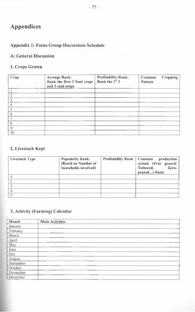
- 7 7 -
Appendices
Appendix 1: Focus Group Discussions Schedule
A: General Discussion
1. Crops Grown
Crop Acreage Rank:Rank the first 3 food crops and 3 cash crops
Profitability Rank: Rank the l “ 3
Common Cropping Pattern
12345678910
2. Livestock Kept
Livestock Type Popularity Rank: (Based on Number of households involved)
Profitability Rank Common production system (Free grazed/ Tethered, Zero- grazed...) Rank
12345
3. Activity (Farming) Calendar
Month Main ActivitiesJanuaryFebruaryMarchAprilMayJuneJulyAugustSeptemberOctoberNovemberDecember
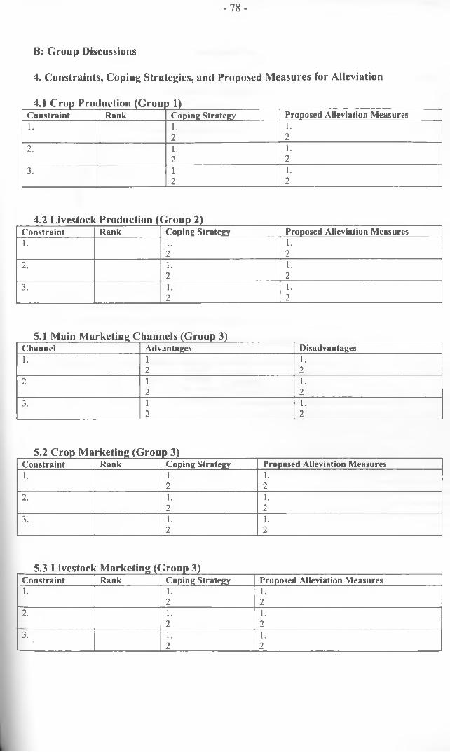
- 7 8 -
B: Group Discussions
4. Constraints, Coping Strategies, and Proposed Measures for Alleviation
4.1 Crop Prod uction (Grou M)Constraint Rank Coping Strategy Proposed Alleviation Measures1. 1. 1.
2 22. 1. 1.
2 23. 1. 1.
2 2
4.2 Livestock Production (Group 2)Constraint Rank Coping Strategy Proposed Alleviation Measures1. 1. 1.
2 22. 1. 1.
2 23. 1. 1.
2 2
5.1 Main Marketing Channels (Group 3)Channel Advantages Disadvantages1. 1. 1.
2 22. 1. 1.
2 23. 1. 1.
2 2
5.2 Crop Marketing (Group 3)Constraint Rank Coping Strategy Proposed Alleviation Measures1. 1. 1.
2 22. 1. 1.
2 23. 1. 1.
2 2
5.3 Livestock Marketing (Group 3)Constraint Rank Coping Strategy Proposed Alleviation Measures1. 1. 1.
2 22. 1. 1.
2 23. 1. 1.
2 2
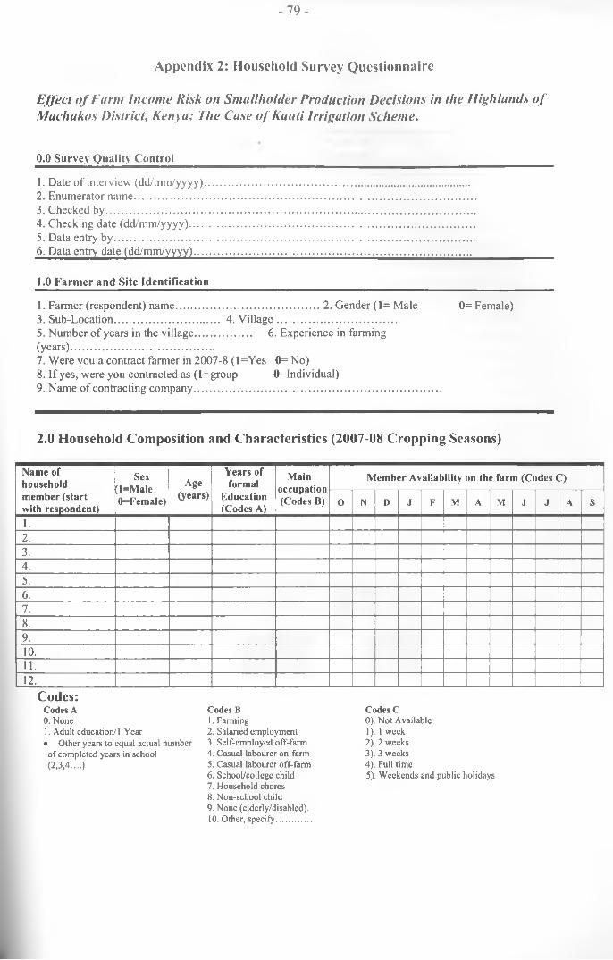
- 7 9 -
A p p en d ix 2: H ou seh o ld S u rvey Q u estio n n a ire
Effect o f Farm Income Risk on Smallholder Production Decisions in the Highlands o f Machakos District, Kenya: The Case o f Kauti Irrigation Scheme.
0. 0.Survey Quality Control_____________________________________________________________
1. Date o f interview (dd/mm/yyyy)...................................................................................................2. Enumerator name................................................................................................................................3. Checked by..........................................................................................................................................4. Checking date (dd/mm/yyyy)..........................................................................................................5. Data entry by......................................................................................................................................6. Data entry date (dd/mm/yyyy).......................................................................................................
1.0 Farmer and Site Identification___________________________________________________
1. Farmer (respondent) name.................................................. 2. Gender (1= Male 0= Female)3. Sub-Location....................................... 4. V illage............................................5. Number o f years in the village..................... 6. Experience in farming(years).....................................................7. Were you a contract farmer in 2007-8 (l=Y es 0= No)8. If yes, were you contracted as (l=group 0=lndividual)9. Name of contracting company............................................................................................
2.0 H ou seh o ld C o m p o sitio n and C h a ra cter istics (2 0 07-08 C ro p p in g S eason s)
N a m e o f h o u s e h o ld m e m b e r ( s ta r t w ith r e s p o n d e n t )
S e x( l= M a le0 = F e m a le )
A g e( y e a r s )
Y e a r s o f fo r m a l
E d u c a t io n (C o d e s A )
M a ino c c u p a t io n ( C o d e s B )
M e m b e r A v a ila b il it y o n th e fa r m ( C o d e s C )
O N D J F M A M J J A S
1.
2 .
3 .
4 .
5 .
6 .
7 .
8 .
9 .
1 0 .
1 1 .
1 2 .
C odes:Codes A Codes B Codes C0. None 1. Farming 0). Not Available1. Adult education/1 Year 2. Salaried employment 1). 1 week• Other years to equal actual number 3. Self-employed off-farm 2). 2 weeksof completed years in school 4. Casual labourer on-farm 3). 3 weeks(2,3,4....) 5. Casual labourer off-farm
6. School/college child7. Household chores8. Non-school child9. None (clderly/disabled).10. Other, specify...............
4) . Full time5) . Weekends and public holidays
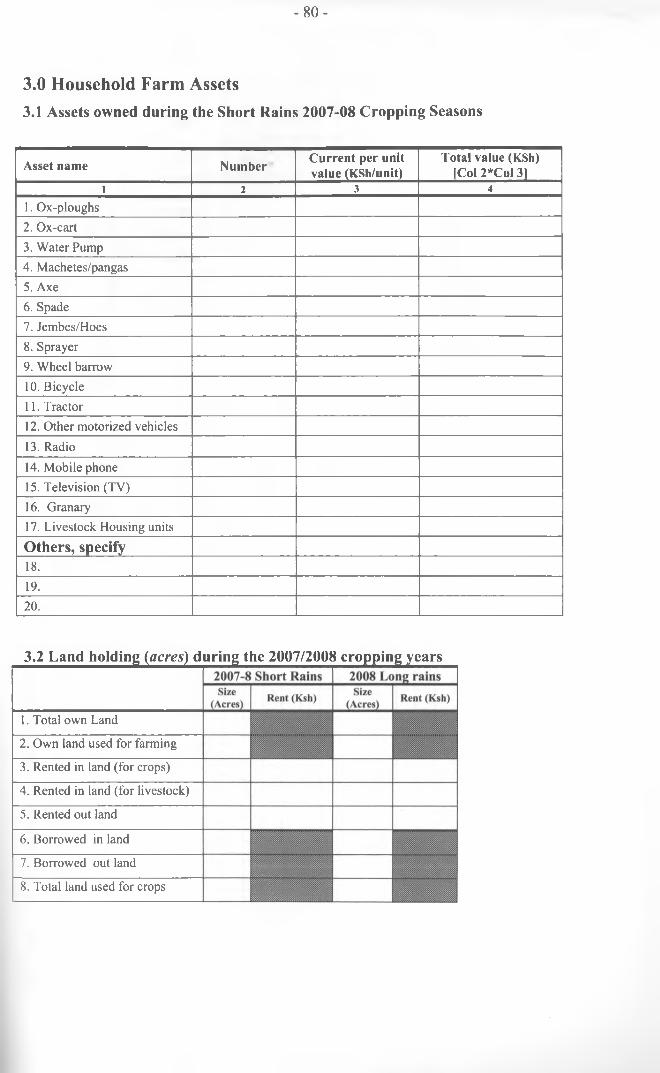
- 8 0 -
3.0 Household Farm Assets3.1 A ssets ow n ed d u rin g the S h ort R ains 2007-08 C ro p p in g S eason s
Asset name Number Current per unit value (KSh/unit)
Total value (KSh) ICol 2*Col 3|
I 2 3 4
1. Ox-ploughs
2. Ox-cart3. Water Pump4. Machetes/pangas
5. Axe6. Spade7. Jembes/Hoes8. Sprayer
9. Wheel barrow10. Bicycle11. Tractor
12. Other motorized vehicles
13. Radio
14. Mobile phone15. Television (TV)
16. Granary17. Livestock Housing units
O th ers, sp ecify18.
19.20.
3.2 L an d h o ld in g (acres) d u r in g the 2 0 0 7 /2008 cro p p in g years
1. Total own Land
2. Own land used for farming
3. Rented in land (for crops)
4. Rented in land (for livestock)
5. Rented out land
6. Borrowed in land
7. Borrowed out land
8. Total land used for crops
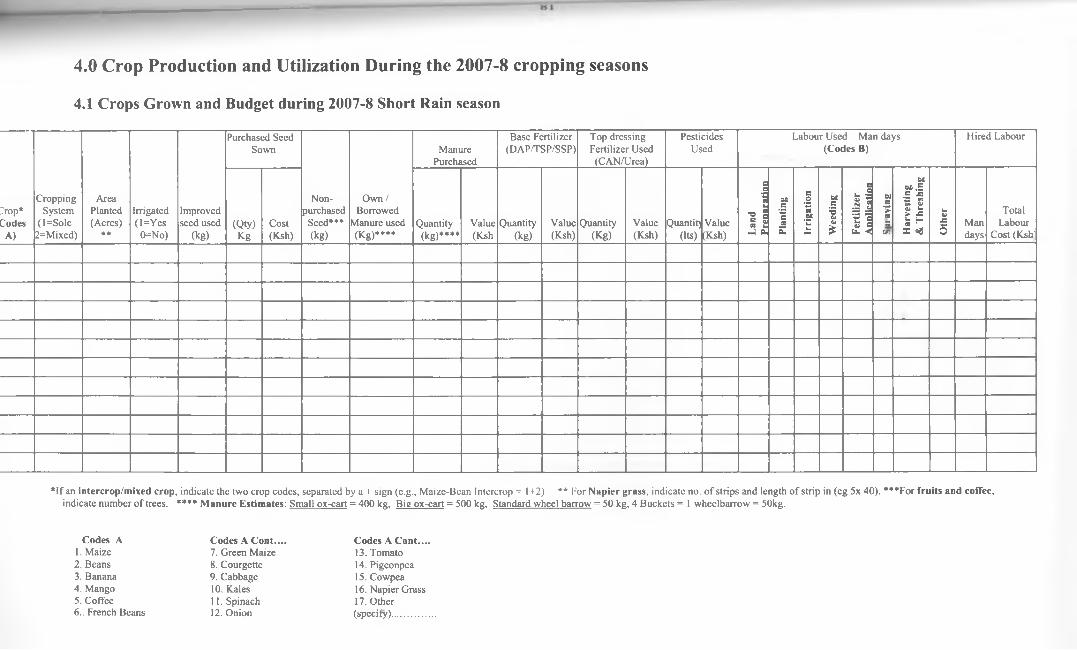
4.0 Crop Production and Utilization During the 2007-8 cropping seasons
4.1 C rop s G row n and B u d get d u rin g 2007-8 S h o rt R ain season
>op*CodesA)
CroppingSystem
(l=Sole2=Mixed)
AreaPlanted(Acres)
**
Irrigated(l=Yes
0=No)
Improved seed used
(kg)
Purchased Seed Sown
Non-purchascdSeed***(kg)
Own / Borrowed
Manure used (Kg)****
ManurePurchased
Base Fertilizer (DAP/TSP/SSP)
Top dressing Fertilizer Used (CAN/Urea)
PesticidesUsed
Labour Used - Man days (Codes B)
Hired Labour
(Q ty)Kg
Cost(Ksh)
Quantity(kg)****
Value(Ksh
Quantity(kg)
Value(Ksh)
Quantity(Kg)
Value(Ksh)
Quantity(Its)
Value(Ksh) L
and
PreD
arat
lon_
_Pl
antin
g
Irri
gatio
n
Wee
ding
Fert
ilize
r A
nnlic
atio
n ___
SIc%SB=C/5 H
arve
stin
g &
Thr
eshi
ng
Oth
er
Mandays
Total Labour
Cost (Ksh'
*If an intercrop/mixed crop, indicate the two crop codes, separated by a + sign (c.g., Maize-Bean Intercrop = I +2) ** For Napier grass, indicate no. of strips and length of strip in (eg 5x 40). ***For fruits and coffee,indicate number of trees. **** Manure Estimates: Small ox-cart = 400 kg, Big ox-cart = 500 kg, Standard wheel barrow = 50 kg, 4 Buckets = 1 wheelbarrow = 50kg.
Codes A1. Maize2. Beans3. Banana4. Mango5. Coffee6.. French Beans
Codes A Cont....7. Green Maize8. Courgette9. Cabbage10. Kales11. Spinach12. Onion
Codes A Cont....13. Tomato14. Pigeonpea15. Cowpea16. Napier Grass17. Other(specify)..............
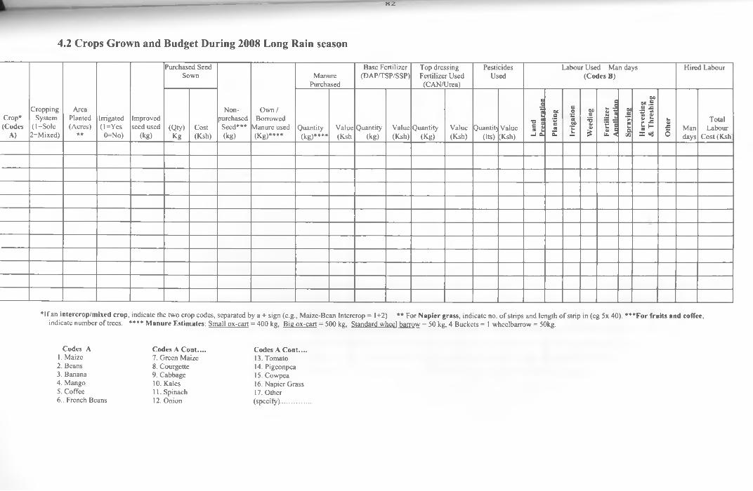
8 2
4.2 C rop s G row n and B u d get D u rin g 2008 L on g R ain season
Crop*(Codes
A)
CroppingSystem
(l=Solc2=Mixed)
AreaPlanted(Acres)
**
Irrigated(l=Ycs
0=No)
Improvedseed used
(kg)
Purchased Seed Sown
Non-purchasedSeed***(kg)
Own / Borrowed
Manure used (Kg)****
ManurePurchased
Base Fertilizer (DAP/TSP/SSP)
Top dressing Fertilizer Used (CAN/Urea)
PesticidesUsed
Labour Used - Man days (Codes B)
Hired Labour
(Qty)Kg
Cost(Ksh)
Quantity(kg)****
Value(Ksh
Quantity(kg)
Value(Ksh)
Quantity(Kg)
Value(Ksh)
Quantity(Its)
Value(Ksh) L
and
Prep
arat
ion_
_Pl
antin
g
Irri
gatio
n
Wee
ding
Fert
ilize
rA
DD
licat
ion
Spra
ving
Har
vest
ing
& T
hres
hing
Oth
er
Mandays
Total Labour
Cost (Ksh
*If an intercrop/mixed crop, indicate the two crop codes, separated by a + sign (c.g., Maize-Bean Intercrop = 1+2) ** For Napier grass, indicate no. of strips and length of strip in (eg 5x 40). ***For fruits and coffee,indicate number of trees. **** Manure Estimates: Small ox-cart = 400 kg, Big ox-cart = 500 kg, Standard wheel barrow = 50 kg, 4 Buckets = 1 wheelbarrow = 50kg.
Codes A1. Maize2. Beans3. Banana4. Mango5. Coffee6.. French Beans
Codes A Cont....7. Green Maize8. Courgette9. Cabbage10. Kales11. Spinach12. Onion
Codes A Cont....13. Tomato14. Pigconpca15. Cowpca16. Napier Grass17. Other(specify)..............
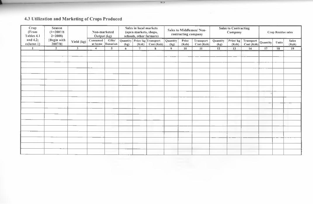
8 3
4.3 U tiliza tion and M ark etin g o f C rop s P rod u ced
Crop (From
T ables 4.1 and 4.2;
colum n 1)
Season (1=2007/8 2=2008)
(Begin with 2007/81
Y ield (kg)
N on-m arketed O utput (kg)
Sales in local m arkets (open m arkets, shops,
schools, other farm ers)
Sales to M iddlem en/ N oncontracting com pany
Sales to C ontracting C om pany Crop Residue sales
Consumed at home
Gifts/Donation
Quantity(kg)
Price/ kg (Ksh)
Transport Cost (Ksh)
Quantity(kg)
Price(Ksh)
Transport Cost (Ksh)
Quantity(kg)
Price/ kg (Ksh)
TransportCost (Ksh) Quantity Units Sales
(Ksh)1 2 3 4 5 6 7 8 9 10 11 12 13 14 17 18 19
•
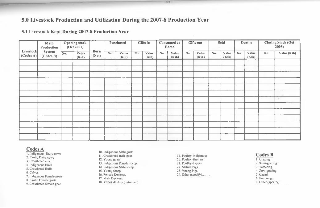
5.0 Livestock Production and Utilization During the 2007-8 Production Year
5.1 L iv esto ck K ep t D u rin g 200 7 -8 P ro d u ctio n Y ear
L ivestock (C odes A)
M ainProduction
System (C odes B)
O pening stock (O ct 2007)
Born(No.)
Purchased G ifts in Consum ed at H om e
G ifts out Sold D eaths C losing Stock (O ct 2008)
No. Value(Ksh)
No. Value(Ksh)
No. Value(Ksh)
No. Value(Ksh)
No. Value(Ksh)
No. Value(Ksh)
No. Value(Ksh)
No. Value (Ksh)
C od es A1. Indigenous Dairy cows2. Exotic Dairy cows3. Crossbreed cow4. Indigenous Bulls5. Crossbreed Bulls6. Calves7. Indigenous Female goats8. Exotic Female goats9. Crossbreed female goat
10. Indigenous Male goats11. Crossbreed male goat12. Young goats13. Indigenous Female sheep14. Indigenous Male sheep15. Young sheep16. Female Donkeys17. Male Donkeys18. Young donkey (untrained)
19. Poultry-Indigenous20. Poultry-Broilers21. Poultry-Layers22. Mature Pigs23. Young Pigs24. Other (specify)......
C o d es B1. Grazing2. Semi-grazing3. Tethering4. Zero-grazing5. Caged6. Free range7. Other (specify).
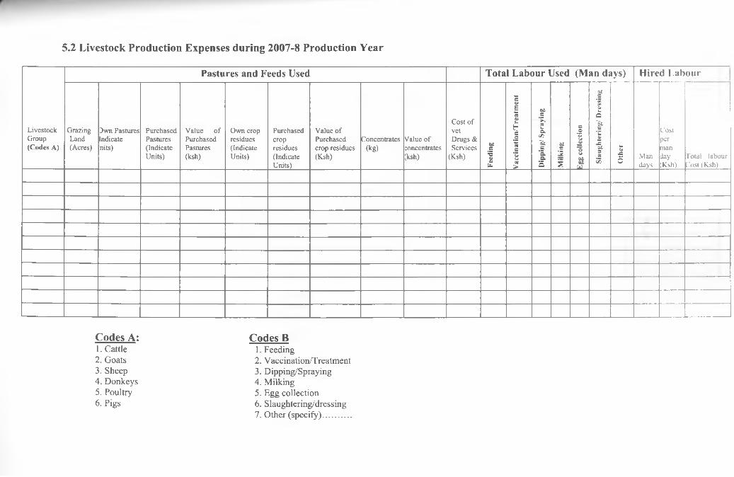
5.2 L iv esto ck P rod u ction E x p en ses d u r in g 200 7 -8 P rod u ction Y ear
Livestock Group (Codes A)
Pastures and Feeds Used Total Labour Used (Man days) Hired Labour
GrazingLand(Acres)
Dwn PasturesIndicatenits)
PurchasedPastures(IndicateUnits)
Value of Purchased Pastures (ksh)
Own crop residues (Indicate Units)
Purchasedcropresidues(IndicateUnits)
Value of Purchased crop residues (Ksh)
Concentrates(kg)
Value ofconcentrates(ksh)
Cost of vetDrugs & Services
(Ksh)
Feed
ing
Vac
cina
tion/
T re
atm
ent
Dip
ping
/ Spr
ayin
g
0£■*J2£ Eg
g co
llect
ion
Slau
ghte
ring
/ Dre
ssin
g
Oth
er
Mandays
Costpermanilay[Ksh)
Total labour Cost (Ksh)
C od es A :1. Cattle2. Goats3. Sheep4. Donkeys5. Poultry6. Pigs
C o d es B1. Feeding2. Vaccination/Treatment3. Dipping/Spraying4. Milking5. Egg collection6. Slaughtering/dressing7. Other (specify).............
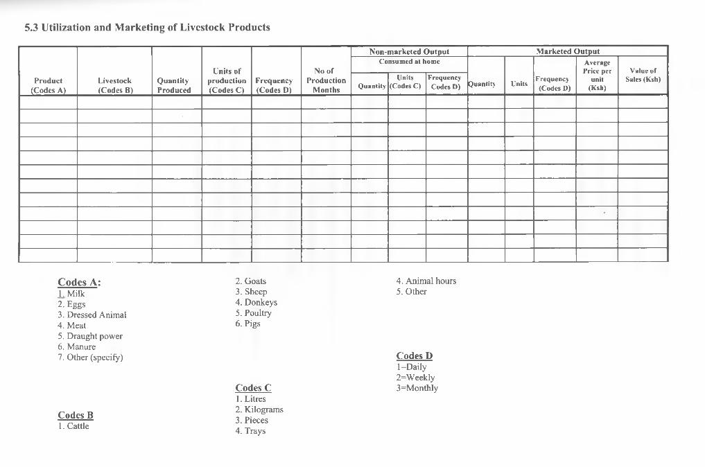
5.3 U tiliza tion and M ark etin g o f L ivestock P rod u cts
Product(Codes A)
L ivestock (C odes B)
Q uantityProduced
Units o f production (C odes C)
Frequency (Codes D)
No of Production
M onths
N on-m arketed O utput M arketed O utputConsumed at home
Quantity UnitsFrequency (Codes D)
Average Price per
unit (Ksh)
Value of Sales (Ksh)
QuantityUnits
(Codes C)Frequency
Codes D)
*
C od es A: 2. Goats 4. Animal hours1. Milk 3. Sheep 5. Other2. Eggs 4. Donkeys3. Dressed Animal 5. Poultry4. Meat 6. Pigs5. Draught power6. Manure7. Other (specify) Codes D
Codes C
l=Daily 2=Weekly 3=Monthly
Codes B
1. Litres2. Kilograms3. Pieces
1. Cattle 4. Trays
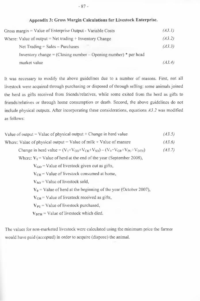
- 87 -
A p p en d ix 3: G ross M argin C a lcu la tio n s for L ivestock E n terp rise .
Gross margin = Value of Enterprise Output - Variable Costs (A3.1)
Where: Value of output = Net trading + Inventory Change (A3.2)
Net Trading = Sales - Purchases (A3.3)
Inventory change = (Closing number - Opening number) * per head
market value (A3.4)
It was necessary to modify the above guidelines due to a number of reasons. First, not all
livestock were acquired through purchasing or disposed of through selling: some animals joined
the herd as gifts received from friends/relatives, while some exited from the herd as gifts to
friends/relatives or through home consumption or death. Second, the above guidelines do not
include physical outputs. After incorporating these considerations, equations A3.2 was modified
as follows:
Value of output = Value of physical output + Change in herd value
Where: Value of physical output = Value of milk + Value of manure
Change in herd value = ( V i + V g o + V c h + V s o ) - ( V 0+ V g r + V p u + V d t h )
Where: Vi = Value of herd at the end of the year (September 2008),
Vgo = Value of livestock given out as gifts,
V c h = Value of livestock consumed at home,
Vso = Value of livestock sold,
Vo = Value of herd at the beginning of the year (October 2007),
Vcr= Value of livestock received as gifts,
Vpt= Value of livestock purchased,
V d t h = Value of livestock which died.
The values for non-marketed livestock were calculated using the minimum price the farmer
would have paid (accepted) in order to acquire (dispose) the animal.
(A3.5)
(A3.6)
(A3.7)
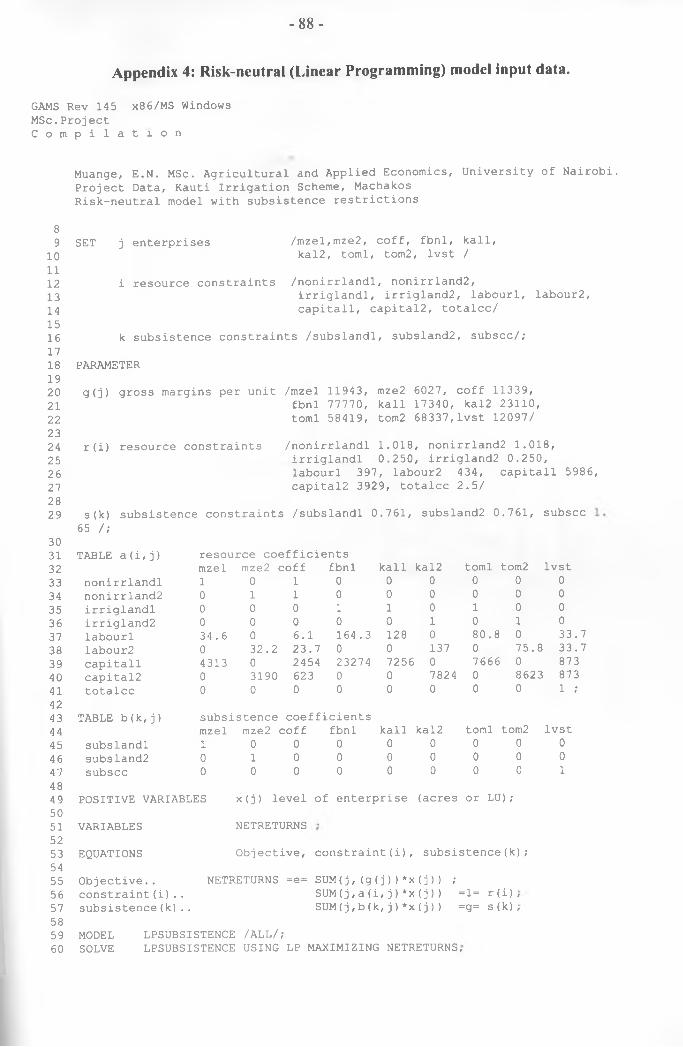
- 88 -
A p p en d ix 4: R isk -n eu tra l (L in ea r P rogram m in g) m odel in p u t data .
GAMS Rev 145 MSc.Project C o m p i 1 a
x86/MS Windows
t 1 o n
Muange, E.N. MSc. Agricultural and Applied Economics, University of Nairobi. Project Data, Kauti Irrigation Scheme, Machakos Risk-neutral model with subsistence restrictions
89
1011121314151617181920 21 2223242526272829
30313233343536373839404142434445464748495051525354555657585960
SET j enterprises /mzel,mze2, coff, fbnl, kail, kal2, toml, tom2, lvst /
i resource constraints /nonirrlandl, nonirrland2,irriglandl, irrigland2, labourl, labour2, capitall, capital2, totalcc/
k subsistence constraints /subslandl, subsland2, subscc/;
PARAMETER
g(j) gross margins per unit /mzel 11943, mze2 6027, coff 11339,fbnl 77770, kail 17340, kal2 23110, toml 58419, tom2 68337,lvst 12097/
r(i) resource constraints /nonirrlandl 1.018, nonirrland2 1.018, irriglandl 0.250, irrigland2 0.250, labourl 397, labour2 434, capitall 5986, capital2 3929, totalcc 2.5/
s(k) subsistencei constraints /subslandl 0.761, subsland2 0.761, subscc65 /;
TABLE a (i,j) resource coefficientsmzel mze2 coff fbnl 1kail kal2 toml tom2 lvst
nonirrlandl 1 0 1 0 0 0 0 0 0nonirrland2 0 1 1 0 0 0 0 0 0irriglandl 0 0 0 1 1 0 1 0 0irrigland2 0 0 0 0 0 1 0 1 0labourl 34.6 0 6.1 164.3 128 0 80.8 0 33.7labour2 0 32.2 23. 7 0 0 137 0 75. 8 33.7capitall 4313 0 2454 23274 7256 0 7666 0 873capital2 0 3190 623 0 0 7824 0 8623 873totalcc 0 0 0 0 0 0 0 0 1 ;
TABLE b(k,j) subsistence coefficientsmzel mze2 coff fbnl kail kal2 toml tom2 lvst
subslandl 1 0 0 0 0 0 0 0 0subsland2 0 1 0 0 0 0 0 0 0subscc 0 0 0 0 0 0 0 0 1
POSITIVE VARIABLES x(j) level of enterprise (acres or LU);
VARIABLES NETRETURNS
EQUATIONS Objective, constraint(i) , subsistence(k);
Objective.. NETRETURNS =e= SUM(j, (g (j))*x (j ) ) ;constraint(i) . . SUM(j,a(i* j)*x (j) ) =1= r(i) !
subsistence(k).. SUM(j,b (k/ j) *x (j )) =g= s(k) •
MODEL LPSUBSISTENCE: /ALL/;SOLVE LPSUBSISTENCE: USING LP MAXIMIZING NETRETURNS/
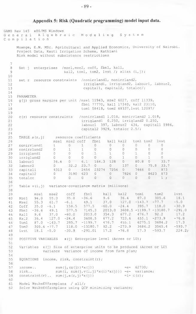
- 89 -
A p p en d ix 5: R isk (Q u a d ra tic p rogram m in g) m odel in p u t data .
GAMS Rev 145 x86/MS WindowsG e n e r a l A l g e b r a i c M o d e l i n g S y s t e m C o m p i l a t i o n
Muange, E.N. MSc. Agricultural and Applied Economics, University of Nairobi. Project Data, Kauti Irrigation Scheme, Kathiani Risk model without subsistence restrictions
78 9
1011121314151617181920 21 222324
5354555657585960 61 62
Set j enterprises /mzel,mze2, coff, fbnl, kail,kal2, toml, tom2, lvst /; alias (i,j);
set r resource constraints /nonirrlandl, nonirrland2,irriglandl, irrigland2, labourl, labour2, capitall, capital2, totalcc/;
PARAMETERg(j) gross margins per unit /mzel 11943, mze2 6027, coff 11339,
fbnl 77770, kail 17340, kal2 23110, toml 58419, tom2 68337,lvst 12097/
c(r) resource constraints /nonirrlandl 1.018, nonirrland2 1.018, irriglandl 0.250, irrigland2 0.250, labourl 397, labour2 434, capitall 5986, capital2 3929, totalcc 2.5/;
25 TABLE a(r,j) resource coefficients26 mzel mze2 icoff fbnl kail kal2 toml tom2 lvst27 nonirrlandl 1 0 1 0 0 0 0 0 028 nonirrland2 0 1 1 0 0 0 0 0 029 irriglandl 0 0 0 i 1 0 1 0 030 irrigland2 0 0 0 0 0 1 0 1 031 labourl 34.6 0 6.1 164 .3 128 0 80.8 0 33.732 labour2 0 32.2 23.7 0 0 137 0 75 .8 33.733 capitall 4313 0 2454 23274 7256 0 7666 0 87334 capital2 0 3190 623 0 0 7824 0 8623 87335 totalcc 0 0 0 0 0 0 0 0 l ;3637 Table v(i,j) variance-covariance matrix (millions)3839 mzel mze2 coff fbnl kail kal2 toml tom2 lvst40 Mzel 94.0 55.3 35.0 -36.6 9.6 36.4 87.0 305.6 18.141 Mze2 55.3 61.7 -6.1 49.1 37 .0 127.0 -143. 7 -77.7 -5.042 Coff 35.0 -6.1 158.5 577. 5 -60 .0 -24.4 395. 7 118.0 -30.943 Fbnl -36.6 49.1 577.5 7145 .3 2013.0 3608.5 -1199 .7 -13180.7 -291.044 Kail 9.6 37.0 -60.0 2013 .0 354.3 677.2 476. 7 92.2 17.245 Kal2 36.4 127.0 -24.4 3608 .5 677.2 723.6 455 .1 -273.9 -76.846 Toml 87.0 -143.7 395.7 -1199 .7 476.7 455.1 6275 .1 3684.2 17.347 Tom2 305.6 -77.7 118.0 -13180.7 92 .2 -273.9 3684 .2 3545.4 -593.748 Lvst 18.1 -5.0 -30.9 -291. 01 17 .2 -76.8 17.3 -593.7 224.24950 POSITIVE VARIABLES x (j) Enterprise level (Acres or LU) ;5152 Variables x (j) Size of enterprise units to be produced (Acres or LU)
variance variance of income from farm plan;
EQUATIONS income, risk, constraint(r);
income.. sum(j, (g(j) ) *x(j ) ) =e= 62730;risk.. sum(i, sum(j , v(i, j)*x(i)*x(j))) =e= variance;constraint(r).. sum(j,a(r,j)*x(j)) =1= c(r);
Model NsubsEVfarmplans / all/;Solve NsubsEVfarmplans using QCP minimizing variance;
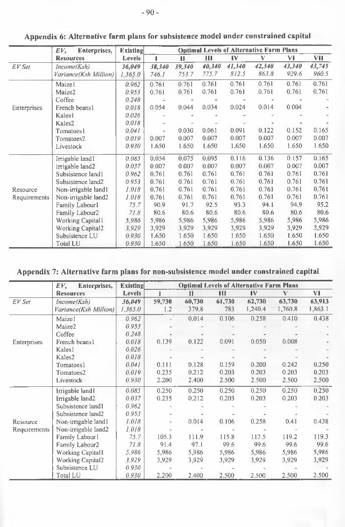
- 9 0 -
A p p en d ix 6: A ltern ative farm p lans for su b sisten ce m odel u n d er co n stra in ed cap ita l
E V , Enterprises, Resources
ExistingLevels
Optimal Levels of Alternative Farm PlansI II III IV V VI VII
E V Set Income(Ksh) 3 6 ,0 4 9 3 8 ,3 4 0 3 9 ,3 4 0 4 0 ,3 4 0 4 1 ,3 4 0 4 2 ,3 4 0 4 3 ,3 4 0 4 3 ,7 4 5Variance(Ksh Million) 1,365.0 746.1 753.7 775.7 812.5 863.8 929.6 960.5
Maize 1 0.962 0.761 0.761 0.761 0.761 0.761 0.761 0.761Maize2 0.953 0.761 0.761 0.761 0.761 0.761 0.761 0.761Coffee 0.248 - - - - - - -
Enterprises French beans 1 0.018 0.054 0.044 0.034 0.024 0.014 0.004 -Kales 1 0.026 - - - - - - -Kales2 0.018 - - - - - - -Tomatoes 1 0.041 - 0.030 0.061 0.091 0.122 0.152 0.165Tomatoes2 0.019 0.007 0.007 0.007 0.007 0.007 0.007 0.007Livestock 0.930 1.650 1.650 1.650 1.650 1.650 1.650 1.650
Irrigable landl 0.085 0.054 0.075 0.095 0.116 0.136 0.157 0.165Irrigable land2 0.037 0.007 0.007 0.007 0.007 0.007 0.007 0.007Subsistence landl 0.962 0.761 0.761 0.761 0.761 0.761 0.761 0.761Subsistence land2 0.953 0.761 0.761 0.761 0.761 0.761 0.761 0.761
Resource Non-irrigable landl 1.018 0.761 0.761 0.761 0.761 0.761 0.761 0.761Requirements Non-irrigable land2 1.018 0.761 0.761 0.761 0.761 0.761 0.761 0.761
Family Labour 1 75.7 90.9 91.7 92.5 93.3 94.1 94.9 95.2Family Labour2 71.8 80.6 80.6 80.6 80.6 80.6 80.6 80.6Working Capital 1 5,986 5,986 5,986 5,986 5,986 5,986 5,986 5,986Working Capital2 3,929 3,929 3,929 3,929 3,929 3,929 3,929 3,929Subsistence LU 0.930 1.650 1.650 1.650 1.650 1.650 1.650 1.650Total LU 0.930 1.650 1.650 1.650 1.650 1.650 1.650 1.650
Appendix 7: Alternative farm plans for non-subsistence model under constrained capital
EV, Enterprises, Resources
ExistingLevels
Optimal Levels of Alternative Farm PlansI II III IV V VI
E V S et Income(Ksh) 36,049 59,730 60,730 61,730 62,730 63,730 63,913Variance(Ksh Million) 1,365.0 1.2 379.8 783 1,240.4 1,760.8 1,863.1Maize 1 0.962 - 0.014 0.106 0.258 0.410 0.438Maize2 0.953 - - - - - -
Coffee 0.248 - - - - - -
Enterprises French beans 1 0.018 0.139 0.122 0.091 0.050 0.008 -
Kales 1 0.026 - - - - - -
Kales2 0.018 - - - - - -
Tomatoes 1 0.041 0.111 0.128 0.159 0.200 0.242 0.250Tomatoes2 0.019 0.235 0.212 0.203 0.203 0.203 0.203Livestock 0.930 2.200 2.400 2.500 2.500 2.500 2.500
Irrigable landl 0.085 0.250 0.250 0.250 0.250 0.250 0.250Irrigable land2 0.037 0.235 0.212 0.203 0.203 0.203 0.203Subsistence landl 0.962 - - - - - -
Subsistence land2 0.953 - - - - - -
Resource Non-irrigable landl 1.018 - 0.014 0.106 0.258 0.41 0.438Requirements Non-irrigable land2 1.018 - - - - - -
Family Labour 1 75.7 105.3 111.9 115.8 117.5 119.2 119.3Family Labour2 71.8 91.4 97.1 99.6 99.6 99.6 99.6Working Capital 1 5,986 5,986 5,986 5,986 5,986 5,986 5,986Working Capital2 3,929 3,929 3,929 3,929 3,929 3,929 3,929Subsistence LU 0.930 - - - - - -
Total LU 0.930 2.200 2.400 2.500 2.500 2.500 2.500
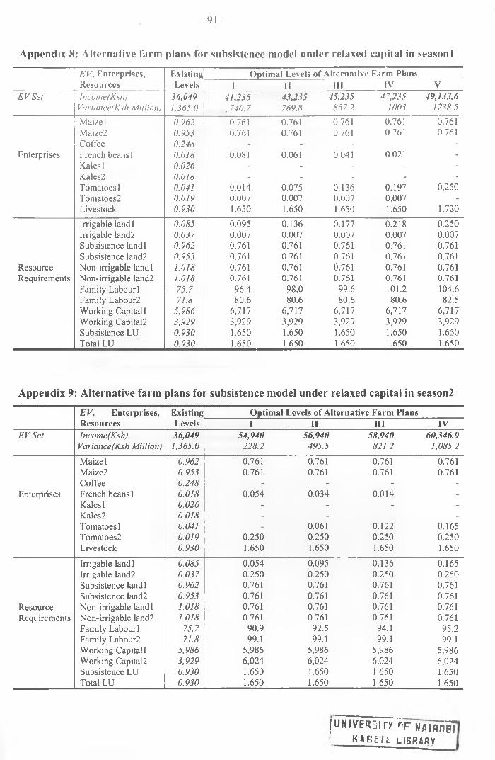
-91 -
A p p en d ix 8: A ltern a tiv e farm p lans for su b sisten ce m odel und er relaxed cap ita l in se a so n l
EV, Enterprises, Resources
ExistingLevels
Optimal Levels of Alternative Farm Plans1 II III IV V
E V S et Income(Ksh) 36,049 41,235 43,235 45,235 47,235 49,133.6Variance(Ksh Million) 1.365.0 , 740.7 769.8 857.2 1003 1238.5
Maize 1 0.962 0.761 0.761 0.761 0.761 0.761Maize2 0.953 0.761 0.761 0.761 0.761 0.761Coffee 0.248 - - - - -
Enterprises French beans 1 0.018 0.081 0.061 0.041 0.021 -Kales 1 0.026 - - - - -Kales2 0.018 - - - - -Tomatoes 1 0.041 0.014 0.075 0.136 0.197 0.250Tomatoes2 0.019 0.007 0.007 0.007 0.007 -
Livestock 0.930 1.650 1.650 1.650 1.650 1.720
Irrigable landl 0.085 0.095 0.136 0.177 0.218 0.250Irrigable land2 0.037 0.007 0.007 0.007 0.007 0.007Subsistence landl 0.962 0.761 0.761 0.761 0.761 0.761Subsistence land2 0.953 0.761 0.761 0.761 0.761 0.761
Resource Non-irrigable landl 1.018 0.761 0.761 0.761 0.761 0.761Requirements Non-irrigable land2 1.018 0.761 0.761 0.761 0.761 0.761
Family Labourl 75.7 96.4 98.0 99.6 101.2 104.6Family Labour2 71.8 80.6 80.6 80.6 80.6 82.5Working Capital 1 5,986 6,717 6,717 6,717 6,717 6,717Working Capital2 3,929 3,929 3,929 3,929 3,929 3,929Subsistence LU 0.930 1.650 1.650 1.650 1.650 1.650Total LU 0.930 1.650 1.650 1.650 1.650 1.650
Appendix 9: Alternative farm plans for subsistence model under relaxed capital in season2
EV, Enterprises, Resources
ExistingLevels
Optimal Levels of Alternative Farm PlansI II III IV
E V S et Income(Ksh) 36,049 54,940 56,940 58,940 60,346.9Variance(Ksh Million) 1,365.0 228.2 495.5 821.2 1,085.2
Maize 1 0.962 0.761 0.761 0.761 0.761Maize2 0.953 0.761 0.761 0.761 0.761Coffee 0.248 - - - -
Enterprises French beans 1 0.018 0.054 0.034 0.014 -
Kales 1 0.026 - - - -
Kales2 0.018 - - - -
Tomatoes 1 0.041 - 0.061 0.122 0.165Tomatoes2 0.019 0.250 0.250 0.250 0.250Livestock 0.930 1.650 1.650 1.650 1.650
Irrigable landl 0.085 0.054 0.095 0.136 0.165Irrigable land2 0.037 0.250 0.250 0.250 0.250Subsistence landl 0.962 0.761 0.761 0.761 0.761Subsistence land2 0.953 0.761 0.761 0.761 0.761
Resource Non-irrigable landl 1.018 0.761 0.761 0.761 0.761Requirements Non-irrigable land2 1.018 0.761 0.761 0.761 0.761
Family Labourl 75.7 90.9 92.5 94.1 95.2Family Labour2 71.8 99.1 99.1 99.1 99.1Working Capital 1 5,986 5,986 5,986 5,986 5,986Working Capital2 3,929 6,024 6,024 6,024 6,024Subsistence LU 0.930 1.650 1.650 1.650 1.650Total LU 0.930 1.650 1.650 1.650 1.650
jUN IVEREITX r t F N m H o i ii K.AEfcii: LI BRARY
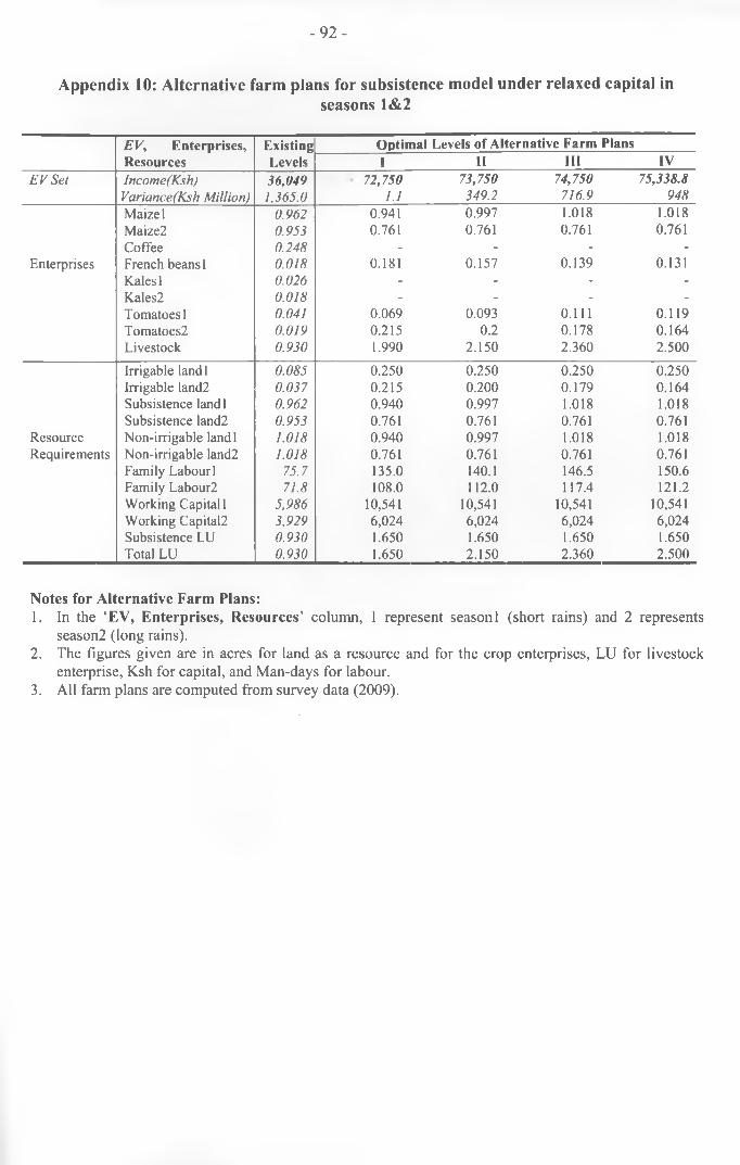
- 9 2 -
Appendix 10: Alternative farm plans for subsistence model under relaxed capital inseasons 1&2
EV, Enterprises, Resources
ExistingLevels
Optimal Levels of Alternative Farm Plans1 II III IV
E V Set Income(Ksh) 36,049 72,750 73,750 74,750 75,338.8Variance(Ksh Million) 1,365.0 1.1 349.2 716.9 948Maize 1 0.962 0.941 0.997 1.018 1.018Maize2 0.953 0.761 0.761 0.761 0.761Coffee 0.248 - - - -
Enterprises French beans 1 0.018 0.181 0.157 0.139 0.131Kales 1 0.026 - - - -Kales2 0.018 - - - -Tomatoes 1 0.041 0.069 0.093 0.111 0.119Tomatoes2 0.019 0.215 0.2 0.178 0.164Livestock 0.930 1.990 2.150 2.360 2.500
Irrigable landl 0.085 0.250 0.250 0.250 0.250Irrigable land2 0.037 0.215 0.200 0.179 0.164Subsistence landl 0.962 0.940 0.997 1.018 1.018Subsistence land2 0.953 0.761 0.761 0.761 0.761
Resource Non-irrigable landl 1.018 0.940 0.997 1.018 1.018Requirements Non-irrigable land2 1.018 0.761 0.761 0.761 0.761
Family Labourl 75.7 135.0 140.1 146.5 150.6Family Labour2 71.8 108.0 112.0 117.4 121.2Working Capital 1 5,986 10,541 10,541 10,541 10,541Working Capital2 3,929 6,024 6,024 6,024 6,024Subsistence LU 0.930 1.650 1.650 1.650 1.650Total LU 0.930 1.650 2.150 2.360 2.500
Notes for Alternative Farm Plans:1. In the ‘EV, Enterprises, Resources’ column, 1 represent seasonl (short rains) and 2 represents
season2 (long rains).2. The figures given are in acres for land as a resource and for the crop enterprises, LU for livestock
enterprise, Ksh for capital, and Man-days for labour.3. A ll farm plans are computed from survey data (2009).