Embed Size (px)
Citation preview

i
EFFECT OF CRUDE OIL CONTAMINATED SAND ON THE
ENGINEERING PROPERTIES OF CONCRETE
BY
WASIU OLABAMIJI AJAGBE
B.Sc, M.Sc (Ibadan)
A thesis in the Department of CIVIL ENGINEERING
Submitted to the Faculty of Technology in partial fulfillment of
the requirement for the Degree of
DOCTOR OF PHILOSOPHY
of the
UNIVERSITY OF IBADAN
Department of Civil Engineering
University of Ibadan
Ibadan
January 2013

ii
ABSTRACT
A considerable fraction of sand in Niger Delta Area of Nigeria is contaminated with
crude oil. The contaminated sand is largely utilised by local contractors for the
production of concrete. However, there is need to establish its suitability in concreting.
Previous works have centered on hardened uncontaminated concrete in crude oil
environment but not on concrete made with Crude Oil Contaminated Sand (COCS).
This research was designed to evaluate the effect of COCS on some engineering
properties of fresh and hardened COCS concrete.
Levels of crude oil contamination were determined using gravimetry method of Total
Petroleum Hydrocarbon (TPH) test on nine sand samples randomly collected from
some oil spill sites in Rivers State. Based on the test results, seven types of artificially
contaminated sand were prepared with crude oil levels of 0.0, 2.5, 5.0, 10.0, 15.0, 20.0
and 25.0%. Workability (slump, compacting factor and flow), compressive strength,
linear shrinkage, water absorption, and fire resistance were determined using concrete
cubes, flexural strength using concrete beams, and surface resistivity using concrete
cylinders in accordance with standard methods. Data obtained were analysed using
ANOVA at p = 0.05. Eight models were developed using historic response surface
methodology to predict the engineering properties of COCS concrete at water-cement
ratio (w/c) of 0.5. Also, COCS concrete design mixes with contamination level and
w/c ratio suitable for reinforced concrete were formulated.
The TPH varied from 8.6 ± 0.2 to 14.1 ± 1.3%. The workability of concrete was
improved by the presence of COCS. Slump, compacting factor and flow of the fresh
concrete increased with increase in contamination from 30.0 to 200.0 mm, 0.5 to 0.9
and 15.0 to 85.0%, respectively. Compressive strength, flexural strength, linear
shrinkage and water absorption of the hardened concrete reduced with levels of
contamination from 31.5 ± 2.3 to 3.5 ± 0.0 N/mm2, 5.9 ± 0.8 to 0.1 ± 0.0 N/mm
2, 0.1 ±
0.0 to 0.0 cm and 0.2 to 0.0 kg respectively. At a temperature of 200.0˚C, the
percentage strength reduction increased from 18.4 to 94.8% for 2.5 to 25.0%
contamination. Surface resistivity ranged from 25.1 ± 0.2 to 32.3 ± 0.2 kΩ-cm. The
compressive and flexural strengths of COCS concrete were reduced by more than
50.0% at crude oil contamination level greater than 10.0%. The water absorption and
surface resistivity values indicated that COCS concrete exhibited greater resistance to
water and chloride penetration respectively, it shrank less when compared with the

iii
uncontaminated concrete, but exhibited poor fire resistance. Coefficient of
determination, R2, of the models developed ranged from 0.823 to 0.999. Concrete
design mix ratio of 1part of cement to1.6 part of COCS (10.0% crude oil) to 2.4 part
of coarse aggregate was found to be appropriate at 0.45 w/c. This mix gave minimum
compressive strength of 21.0 N/mm2 which is acceptable for reinforced concrete
structures.
Concretes produced with sand contaminated with less than ten percent crude oil were
found suitable for use in low strength structures. Mix re-design using lower w/c
improved the strength of the concrete.
Keywords: Crude oil-contaminated sand, Concrete properties, Compressive strength.
Word count: 498

iv
DEDICATION
This thesis is dedicated to my late father, and brothers and sisters on the path of
ALLAH.

v
ACKNOWLEDGEMENT
I give thanks and praises to ALLAH for His Mercies, Protection and Guidance
over me from birth till date; and most importantly for keeping my feet firm on the path
of rectitude. I seek Allah’s Blessing on the soul of our noble prophet Muhammed
(SAW), his house hold and the generality of the muslim community.
I wish to appreciate sincerely my supervisors for their unrelenting efforts
toward the successful completion of this research programme. First to mention is Dr S.
O. Franklin who set the stage for the progamme, followed by Dr G. A. Alade who for a
long time was with me through the thick and thin of the struggle, I thank you for your
physical and spiritual supports. Prof. O. A. Agbede, my all time supervisor (B. Sc., M.
Sc. and Ph.D.)! I thank you for your consistent encouragement from inception till date
and finally is Dr B. I. O. Dahunsi for his timely intervention to see to the completion of
this programme.
I am indebted to all my senior colleagues in the department-Prof. A. O. Coker,
Dr F. Olutoge, Dr W. K. Kupolati, Dr G. M. Ayininuola Mrs E. Adebamowo, Dr
Folake Akintayo, and Dr. Joy Oladejo. The contributions of my colleagues in the
Faculty of Technology are worth mentioning. I specifically appreciate the
contributions of Prof. M. A. Onilude, Prof. A. Olorunnisola, Dr R. Akinoso, Prof. A.
O. Raji, Prof. R. Oloyede, Dr A.S.O. Ogunjuyigbe, Dr Ewemoje, Dr Dare, Dr Zubair,
Dr O. S. Ismail, Dr V. Oladokun, Dr M. T. Lamidi of department of English, U.I., Dr
S. Amidu, and Mr A. Ganiyu. I enjoyed the systemic support and encouragement from
the Dean of the faculty of Technology, Prof. A. E. Oluleye, thanks sir. I wish to
acknowledge the support of Alhaja T. Muritala and all the non teaching staffs in the
department of Civil Engineering, U. I.
Very special thanks go to those that gave my research financial and technical
supports-Engr. S. A. J. Adepoju, Engr. O. Labiran, Engr. Titilola Imran, Engr. W. K.
Aremu, McArtur Foundation, Petroleum Trust Development Fund (PTDF), Academic
Staff Union of Universities (ASUU), and the Postgraduate School, University of
Ibadan.
I thank my project students: Omokehinde Olusola, Olapade Kafayat, Pronen
Gabriel, Akong-Egozi Samuel, Ozulu David, Rabiu Wasiu, Odufuwa Omodayo, and
Owoyele Michael, for their cooperation and supports toward the success of the
research.

vi
My unreserved appreciations go to well wishers: Staffs of OSOT Associates,
Johnak Engineering, staffs of department of Civil Engineering, LAUTECH and The
Polytechnic Ibadan, 2011-2013 Exco members of NSE, Ibadan Branch, members of
Muslim community, U. I. and other individuals too numerous to mention.
Special thanks to my brothers and sisters in faith. My families, particularly my
mother, are appreciated for their understanding and support. The understanding and
supports of my dear wife, Rahmat Olayinka and my daughters: Ameenah, Sofiyyah,
Sumayyah and Aisha, are very much appreciated.

vii
CERTIFICATION
I certify that this work was carried out by W. O. Ajagbe in the Department of
Civil Engineering, Faculty of Technology, University of Ibadan.
--------------------------------------------------------
Supervisor
Prof. O. A. Agbede
B. Sc., M. Sc. (Ife), Ph.D. (London), MNSE
MNSE, MNMGS, MNAH, MIWEM, MAGID
Professor of Civil Engineering
Department of Civil Engineering,
University of Ibadan, Nigeria
--------------------------------------------------------
Supervisor
Dr. B.I.O Dahunsi
B. Sc. (Ife), M. Sc., Ph.D. (Ibadan)
MNSE, AMASCE, M.INEnv, Reg. Engr. (COREN)
Senior Lecturer, Department of Civil Engineering,
University of Ibadan, Nigeria

viii
TABLE OF CONTENTS
TITLE PAGE i
ABSTRACT ii
DEDICATION iv
ACKNOWLEDGEMENT v
CERTIFICATION vii
TABLE OF CONTENT viii
LIST OF TABLE S xii
LIST OF FIGURES xiii
LIST OF PLATES xiv
CHAPTER ONE: INTRODUCTION
1.1. Background to the Research 1
1.2 Research Problems 5
1.3. Research Objectives 5
1.4. Justification of Research 6
1.5. Scope of Research 6
1.6 . Area of Study 6
CHAPTER TWO: LITERATURE REVIEW
2.1. Concrete 10
2.2. Concrete Materials/Composition 10
2.3. Properties of Concrete 12
2.3.1. Fresh Concrete 12
2.3.1.1. Workability and its measurement 12
2.4. Concrete in its Hardened State 13
2.4.1. Concrete Strength 14
2.4.1.1. Effects of Mixing Water on Concrete Strength 15
2.4.1.2. Effects of Water/Cement Ratio on Concrete strength 15
2.4.1.3. Influence of Properties of Coarse Aggregate on Strength of Concrete 16
2.4.1.4. Effects of Aggregate/Cement Ratio on Concrete Strength 17
2.4.1.5. Concrete Strength in Tension 18
2.4.1.6. Influence of Early Temperature on Concrete Strength 18
2.4.1.7. Flexural Strength Test of Concrete 19

ix
2.4.2. Durability of concrete 19
2.4.2.1. Significance of Durability 20
2.4.2.2. Strength and Durability Relationship 22
2.4.2.3. Volume Change in Concrete 23
2.4.2.4. Permeability of concrete 24
2.4.2.5. Fire Resistance of concrete 25
2.5. Crude Oil 26
2.5.1. Nigeria Oil Coastal Area 27
2.5.2. Oil spills and its consequencies 27
2.6. Contamination 29
2.6.1. Concrete in hydrocarbon product environment 30
2.6.2. Effect of crude oil on concrete 32
2.7. Modelling of Concrete Properties and Optimization 34
CHAPTER THREE: METHODOLOGY
3.1. Materials 37
3.1.1. Cement 37
3.1.2. Water 37
3.1.3. Coarse aggregate 37
3.1.4. Fine aggregate 37
3.1.5. Crude oil 37
3.1.6. Contaminated sand 37
3.2. Sample Preparation 38
3.2.1. Aggregate 38
3.2.2. Contaminated sand 38
3.2.3. Contamination of Sand with Crude Oil 38
3.3. Materials Testing 42
3.3.1. Cement 42
3.3.2. Water 42
3.3.3. Aggregates 42
3.3.4 Extraction of crude oil 43
3.4. Concrete Mix Design 44
3.4.1. British Method of Concrete Mix Design 44
x
3.5. Production of Concrete 45
3.6. Concrete Test Procedures 47
3.6.1. Tests on Fresh Concrete 47
3.6.1.1. Slump test 47
3.6.1.2. Compacting factor test 48
3.6.1.3. Flow Table test 50
3.6.2. Tests on Hardened Concrete 51
3.6.2.1. Strength tests 51
3.6.2.1.1 Compressive strength test 54
3.6.2.1.2. Flexural Strength (Modulus of Rupture) Test 54
3.6.2.2. Durability tests 56
3.6.2.2.1. Water absorption test 56
3.6.2.2.2. Shrinkage test 58
3.6.2.2.3. Surface Resistivity indication of concrete’s ability to resist
Chloride ion penetration 58
3.6.2.2.4. Fire Resistance test 59
3.7. Experimental Control 59
3.7.1. Casting of Concrete Sample 59
3.8. Development of Models 60
3.8.1. Design Summary for Compressive Strength Model 60
3.8.2. Design Summary for Other Properties 60
3.9. Mix Proportioning for High Strength COIS Concrete 65
CHAPTER FOUR: RESULTS AND DISCUSSION
4.1. Results of Preliminary Studies 67
4.1.1. Sieve analysis 67
4.1.2. Result of Total Petroleum Hydrocarbon (TPH) 67
4.2. Results and Discussions of Tests on Concrete Samples 74
4.2.1. Results of tests on fresh concrete 74
4.2.1.1. Slump test 74
4.2.1.2. Compacting Factor test 74
4.2.1.3. Result of Flow Table test 74
4.2.2. Effect of COCS on the fresh properties of concrete 78
4.3. Results and Discussions of Tests on Hardened Concrete 78

xi
4.3.1. Strength test results 78
4.3.1.1. Compressive strength test results 78
4.3.1. 2. Flexural strength test results 81
4.3.2. Effect of COCS on the strength of concrete 81
4.3.3. Durability test results 82
4.3.3.1. Water absorption test result 82
4.3.3.2. Shrinkage test result 82
4.3.3.3. Concrete Electrical Resistivity test result 86
4.3.3.4. Fire Resistance test result 86
4.3.4. Effect of COCS on the durability of concrete 90
4.4. Mathematical Models 90
4.4.1. Compressive Strength Model 90
4.4.2. Models for Other Properties 91
4.5. Mix Proportioning Compressive Strength Test Result 99
CHAPTER FIVE: CONCLUSIONS AND RECOMMENDATIONS
5.1. Conclusions 102
5.2. Recommendations 103
REFERENCES 104
APPENDICES 114

xii
LIST OF TABLES
Table 3.1. Mix Proportions of Materials 48
Table 3.2. Experimental Factor Input for Compressive Strength 63
Table 3.3. Measured Response Input for Compressive Strength 64
Table 3.4. Experimental Factor Input for Other Properties 65
Table 3.5. Measured Response Input for Other Properties 66
Table 3.6. Mix Proportion of Materials 68
Table 4.1. TPH Test Results 75
Table 4.2. Results of Slump Test 77
Table 4.3. Results of Compacting Factor Test 78
Table 4.4. Result of Flow Table Test 79
Table 4.5. Flexural Strength Test Results 85
Table 4.6. Water Absorption Test Results 86
Table 4.7. Shrinkage Test Result 87
Table 4.8. Chloride Ion Penetrability Based 89
Table 4.9. Concrete Surface Resistivity Test Results 90
Table 4.10. Compressive Strength of Heated COIS Concrete Cubes 91
Table 4.11. Input Details Showing Factors and Response 94
Table 4.12. Model Summary Statistics 96
Table 4.13. Input Parameters for the Responses and the Model Type 99
Table 4.14. Statistical Models for the other Responses 100
Table 4.15. Compressive Strength for Different Mix Proportions 102
Table 4.16. Designed Mix Ratios and their 28 days Compressive Strength 103

xiii
LIST OF FIGURES
Fig. 1.1. Map Showing Area of Study 8
Fig. 1.2. Map Showing Sample Locations in Gokana Local Government Area 9
Fig. 4.1. Particle Size Distribution Curve of Bodo Spill Location 70
Fig. 4.2. Particle Size Distribution Curve of Bomu Spill Location 71
Fig. 4.3. Particle Size Distribution Curve of B-Dere Spill Location 72
Fig. 4.4. Particle Size Distribution Curve of Uncontaminated Fine Aggregate 73
Fig. 4.5. Particle Size Distribution Curve of Coarse Aggregate 74
Fig. 4.6. Compressive Strength Development of Concrete 81
Fig. 4.7. Percentage Reduction of Compressive Strength of Concrete Cubes 82
Fig. 4.8. Comprssive Strength Measured Values Vs Predicted Values 97
Fig. 4.9. Response Surface for Desirability Effects of Variables Interactions 98

xiv
LIST OF PLATES
Plate 3.1. Oil Spill Location at B-Dere 41
Plate 3.2. Oil Spill Location at Bomu 42
Plate 3.3. Oil Spill Location at Bodo 43
Plate 3.4. Preparing Soil Sample for TPH Test 74
Plate 3.5a. Measuring of the Slump of a Contaminated Concrete 51
Plate 3.5b. The Slump of a Contaminated Concrete 51
Plate 3.6a. The Compacting Factor Apparatus Ready for Use 54
Plate 3.6b. Compacting Factor Test in Progress 54
Plate 3.7a. Flow Table (Locally fabricated) Test in Progress 55
Plate 3.7b. Spread of Concrete being measured in a Flow Table Test in Progress 55
Plate 3.8. Cube in a Compression Machine Ready for Crushing 57
Plate 3.9a. Concrete Beams after Curing Ready for Weighing 59
Plate 3.9b. Concrete Beams in Universal Machine being inspected prior
to Flexural Test 59

CHAPTER ONE
INTRODUCTION
1.1 Background to the Research
Petroleum is a critically important but nonrenewable natural resource. It is a
complex, naturally occurring mixture of organic compounds that is produced by the
incomplete decomposition of biomass over a geologically long period of time. Petroleum
compounds can occur in a gaseous form that is often called natural gas, as a liquid called
crude oil, and as a solid or semisolid asphalt or tar associated with oil sands and shale
(Nigerian Environmental Study/Action Team, 1991). Both crude oil and natural gas are
predominantly a mixture of hydrocarbons (Wikipedia, 2010). Crude oil is a dark, sticky
liquid which can be distilled or refined to make fuels, lubricating oils, asphalts and other
valuable products. Because most petroleum is extracted in locations that are remote from
places where consumption occurs, it is a commodity that must be transported in a very
large quantity. The most important methods of transportation are by oceanic tanker and
overland pipeline. These transportation methods can pollute the environment by accidental
oil spills and by operational discharge (i.e. the cleaning of storage and ballast tanks).
One of the problems that characterize oil producing communities in Nigeria is that
of oil spillage. It is a major environmental concern in the Niger Delta where over 80% of
the country‘s crude oil is produced. Other areas are not left out as oil spills occur as a
result of pipeline vandalism and inadequate care on oil production operations. Thousands
of barrels of oil have been let loose into the environment through oil pipelines and tanks in
the country. Between 1976 and 1996, Nigeria recorded a total of 4,835 oil spill incidents,
which resulted in a loss of 1,896,960 barrels of oil to the environment (Nwilo and Badejo,
2004). Oil spill has led to very serious pollution of lands and water in such areas. Some
major spills in the coastal zone are the Gulf Oil Company of Nigeria‘s (GOCON)
Escravos spill in 1978 of about 300,000 barrels, Shell Petroleum Development Company
of Nigeria‘s (SPDC- a subsidiary of the Royal Dutch Shell) Forcados terminal tank failure
in 1978 of about 580,000 barrels and Texaco Funiwa-5 blow out in 1980 of about 400,000
barrels. Other oil spill incidents are those of the Abudu pipeline in 1982 of about 18,818

2
barrels (Niger Delta Environmental Survey (NDES), 1997). Others are Jesse fire incident
which claimed about a thousand lives and the Idoho oil spill of January 1998, of about
40,000 barrels. The most publicized of all oil spills in Nigeria occurred on January 17,
1980 when a total of 37.0 million litres of crude oil got spilled into the environment. The
heaviest recorded spills so far occurred in 1979 and 1980 with a net volume of 694,117.13
barrels and 600,511.02 barrels respectively (Nwilo and Badejo, 2004). An estimated 9 to
13 million barrels (1.5 million tons) of oil has spilled in the Niger Delta ecosystem over
the past 53 years, representing about 50 times the estimated volume spilled in the Exxon
Valdez Oil Spill in Alaska in 1989 (Leschine, et al., 1993; Weiner et al., 1997).
The harmful effects of oil spill on the environment are many. Oil kills plants and
animals in the estuarine zone. Oil settles on beaches and kills organisms that live there; it
also settles on ocean floor and kills benthic (bottom-dwelling) organisms such as crabs.
Oil poisons algae, disrupts major food chains and decreases the yield of edible
crustaceans. It also coats birds, impairing their flight or reducing the insulative mm,
property of their feathers, thus making the birds more vulnerable to cold. Oil endangers
fish hatcheries in coastal waters and as well contaminates the flesh of commercially
valuable fish. In a bid to clean oil spills by the use of oil dispersants, serious toxic effects
will be exerted on plankton thereby poisoning marine animals. This can further lead to
food poisoning and loss of lives. Another effect of oil slicks is loss of economic resources
to the government when spilled oil is not quickly recovered, it will be dispersed abroad by
the combine action of tide, wind and current. The oil will therefore spread into thin films,
dissolve in water and undergo photochemical oxidation, which will lead to its
decomposition. Oil spill has also destroyed farmlands, polluted ground and drinkable
water and caused drawbacks in fishing off the coastal waters (Nwilo and Badejo, 2008).
Over the past two decades, the amount of hydrocarbon contamination of soil and
environment has continually increased, and presently it constitutes a significant fraction of
waste materials in the environment. It has been reported that the presence of
contamination (organic or inorganic) greatly influences the quality of soil (an essential
component of concrete), as they are either attached physically or chemically to the soil
particles or trapped in the voids between the particles.
3
Concrete is a mixture of water, stone (fine and coarse aggregates) and a binder,
nowadays usually Portland cement, which hardens to a stone-like mass (Scott, 1991).
The binder which is made up of cement and water are key ingredients. When cement and
water are mixed they form a paste that binds the aggregates together. The water needs to
be pure in order to prevent side reactions from occurring as this may weaken the concrete
or otherwise interfere with the hydration process. The role of water is important because
the water to cement ratio is the most critical factor in the production of ‗perfect‘ concrete.
Too much water reduces concrete strength, while too little will make the concrete
unworkable. Concrete needs to be workable so that it may be consolidated and shaped into
different forms. Because concrete must be both strong and workable, a careful balance of
the water to cement ratio is required when making concrete.
The filler which constitutes fine aggregate (sand) is made up of particles which can
pass through 5 mm BS 410 test sieve and coarse aggregates larger than 5 mm BS 410 test
sieve. Aggregates should be clean, hard, and well graded, without natural cleavage planes
such as those that occur in slate or shale. The quality of aggregates is very important since
they make up about 60 to 75% of the volume of the concrete; it is impossible to make
good concrete with poor aggregates. The grading of both fine and coarse aggregates is
very significant because having a full range of sizes reduces the amount of cement paste
needed. Well-graded aggregates tend to make the mix more workable as well (Neville,
1993).
The relative quantities of the mixture of concrete ingredients control its properties
in wet or green state as well as in hardened state. Concrete making is not just a matter of
mixing ingredients to produce a plastic mass, but good concrete has to satisfy performance
requirements in the plastic or green state and also the hardened state. In the plastic state
the concrete should be workable and free from segregation and bleeding. In its hardened
state concrete should be strong, durable, and impermeable; and it should have minimum
dimensional changes (Gambhir, 2005).
In general, compressive strength is considered to be the most important property
and the quality of concrete is often judged by its strength (Gambhir, 2005; Shetty, 2002;
Gupta and Gupta, 2004; Mehta and Monteiro, 2006). There are, however, many occasions
when other properties are more important. For example, low permeability and low

4
shrinkages are required for water retaining structures. Although, in most cases an
improvement in compressive strength results in an improvement of the other properties of
concrete, there are exceptions. For example, increasing the cement content of a mix
improves compressive strength but results in higher shrinkage which in extreme cases can
adversely affect durability and permeability. Since the properties of concrete change with
age and environment it is not possible to attribute absolute value to any of them.
The compressive strength of concrete depends on the properties of its ingredients,
the proportion of mix, the method of compact, the presence of contaminants and their
degree and other controls during placing and curing. One very important factor that affects
the compressive strength is contaminant and their degree. The ingredients of concrete are
naturally contaminated, and by man‘s activities but the extent or degree of contamination
may differ from the ingredient source. These may be silica, sea water (salts), clay
minerals, anaerobic bacteria, chlorides, sulphates (sulfates), crude oil (hydrocarbon)
contaminants etc. The presence of contaminant in large degree in aggregates does not only
affect the appearance of concrete (in terms of colour and smell) but also the strength
developed by the concrete and its durability (British Cement Association, 2001).
Durability is a very important concern in using concrete for a given application.
Concrete provides good performance through the service life of the structure when
concrete is mixed properly and care is taken in curing it. Good concrete can have a long
life span under the right conditions. Water, although important for concrete hydration and
hardening, can also play a role in decreasing durability once the structure is built. This is
because water can transport harmful chemicals to the interior of the concrete leading to
various forms of deterioration.
Considering therefore, the influence of ‗clean‘ soil in preserving concrete
properties, and the overall significance of quality and acceptable concrete to the
construction industry, it is imperative to conduct a study to examine such factors that
threatens the achievement of the desired workability, strength and durability of concrete.
The contaminant in focus is crude oil on sand and its effect on the fresh and hardened
properties of concrete are examined in this research. Three areas, Bodo, B-Dere and
Bomu, in Gokana Local Government of Rivers State of the Niger Delta were used as
reference for gathering background data for the research.

5
1.2. Research Problems
The establishment of Niger Delta Development Commission (NDDC) have been
encouraging the construction of concrete structures of various kinds in the area towards
the actualization of Niger Delta Region Development Master Plan (NDRDMP). In some
areas, it may be difficult to obtain sufficient quantities of uncontaminated fine aggregates
but contaminated aggregates are available. Therefore, the occasional use of contaminated
aggregates for construction purposes, particularly by the local contractors, has to be
considered. The agony of building collapses among all other things has become an
endemic plague constantly striking in recent years in this country without it being properly
addressed and prevented. Hence, the unconditional use of crude oil contaminated sand in
the production of concrete must be subjected to tests and its suitability validated. In
addition, reclamation of polluted site is the best form of cleaning the environment, thus a
research into the effect of Crude Oil Contaminated Sand (COCS) on the properties of
concrete poise to find a use for the contaminated material, and, in return, produce a
marketable good that can offset the environmental cleaning cost.
1.3. Research Objectives
The general objective of this research is to investigate the effect of COCS on the
engineering properties of concrete. The specific objectives are as follows:
1) To investigate the percentage of Total Petroleum Hydrocarbon (TPH) in
the sands of three contaminated sites.
2) To determine the effect of COCS on the workability of fresh concrete.
3) To determine the effect of COCS on the strength and durability of hardened
concrete.
4) To develop mathematical model for the fresh and hardened properties of
COCS concrete.
5) To design mix proportions for improved compressive strength of COCS
concrete.

6
1.4. Justification of Research
Concrete being the most widely used construction materials, is also the material of
choice where strength, permanence, durability, impermeability, fire resistance and
abrasion resistance are required (Newman, 2003). The use of this material is inevitable in
a crude oil polluted environment such as in the Niger Delta. Therefore, a research into the
effect of COCS on the properties of concrete will bring about the following:
a) Reclamation of the contaminated areas.
b) Inculcation of necessary factors of safety into the design of reinforced concrete
structures in the polluted areas.
c) Utilization of the COCS concrete in special circumstances, following the
knowledge of the effect that COCS has on some properties of concrete.
d) Establishment of the effect of COCS when used as concrete material in concrete
structures, unlike the effect of crude oil on concrete structures in a crude oil
polluted environment which had been largely considered in previous researches.
1.5 Scope of Research
The study was carried out using dead (stored) crude oil as the hydrocarbon
contaminant in sand. Where more than one test is available for a particular concrete
property, the most relevant of the tests to this research was considered, in addition to
availability of test apparatus. Only the fine aggregate component of concrete was
contaminated with crude oil, prior to concrete production.
1.6. Area of Study
While oil was first discovered in commercial quantity in 1956 in Oloibiri town in
the present day Bayelsa State, the second discovery of oil in commercial volume was at
Bomu in 1958. The Bomu oil field contributed major supply to the first shipment of oil
from Nigeria in 1958. Bomu in Ogoni town is administratively located in Gokana Local
Government Area (LGA) of Rivers state. There are 96 oil wells connected to the five flow
stations in Ogoni, operated by SPDC. Three of the Ogoni flow stations named Bomu, B-

7
Dere and Bodo West are situated in Gokana LGA and constituted the area of study for this
research (Fig. 1.1).
Gokana LGA is among the 23 LGAs in Rivers State of Nigeria. It was created out
of Gokana/Tai/Eleme LGA in September 23, 1991. The council head quarter is located in
Kpor. The LGA is located within the South-East Senatorial District of the state and has
both riverine and upland communities.
The LGA is bounded in the North by Tai LGA, in the East by Khana LGA, in the
West by Ogu/Bolo Local Government Area, in the South by Bonny LGA and in the South
– East by Andoni LGA. Gokana is about 50km south of Port Harcourt and 30km from the
Onne industrial axis. It is blessed with large expanse of mangrove and thick rain forest.

8
Fig. 1.1. Map Showing Area of Case Study, Rivers State, Nigeria

9
Fig. 1.2. Map Showing Sample Locations in Gokana Local Government Area
B Dere
Bomu
Bodo

10
CHAPTER TWO
LITERATURE REVIEW
2.1 Concrete
Concrete is a composite material composed of coarse granular material (the
aggregate or filler) embedded in a hard matrix of material (the cement or binder) that fills
the space between the aggregate particles and glues them together. Concrete can also be
considered as a composite material that consists essentially of a binding medium within
which are embedded particles or fragments of aggregates (Sun et al., 2007). West (2002)
observed that concrete can be defined completely by two parameters, namely its yield
value (the stress is required to get concrete to flow) and its plastic viscosity (how ‘runny‘
it is when it does flow). Concrete can be reliably and repeatably characterised using these
two parameters, to a high degree of accuracy, such that that any change to the concrete
constituents can be diagnosed with some confidence. Concrete is the most versatile
material of construction the world over. It has achieved the distinction of being the
―largest man-made material‖ with the average per capita consumption exceeding 2 kg.
Concrete is the material of choice for a variety of applications such as housing, bridges,
highway pavements, industrial structures, water-carrying and retaining structures, etc. The
credit for this achievement goes to well-known advantages of concrete such as easy
availability of ingredients, adequate engineering properties for a variety of structural
applications, adaptability, versatility, relative low cost, etc. Moreover, concrete has an
excellent ecological profile compared with other materials of construction (Kulkarni,
2009). Shetty (2002), opined that cement concrete is one of the seemingly simple but
actually complex materials. Many of its complex behaviours are yet to be identified to
employ this material advantageously and economically. The behaviour of concrete with
respect to long-term drying shrinkage, creep, fatigue, morphology of gel structure, bond,
fracture mechanism, and polymer modified concrete, and fibrous concrete are some of the
areas of active research in order to have a deeper understanding of the complex behaviour
of this material.
Concrete is a site-made material unlike other materials of construction and as such
can vary to a very great extent in its quality, properties and performance owing to the use

11
of natural materials except cement. From materials of varying properties, to make
concrete of stipulated qualities, an intimate knowledge of the interaction of various
ingredients that go into the making of concrete is required, both in the plastic condition
and in the hardened condition (Shetty, 2002). In addition, Neville and Brooks (1990)
observed that concrete has to be satisfactory in its hardened state and also in its fresh state.
Generally, the requirements in the fresh state are that the consistency of the mix is such
that the concrete can be compacted and that the mix is cohesive enough to be transported
and placed without segregation by the means available. As far as the hardened state is
concerned, the usual requirement is a satisfactory comprehensive strength.
2.2. Concrete Materials/Composition
Concrete composition refers to the various constituents or ingredients that are
needed in varying proportions for the production of concrete. These are cement, fine
aggregate, coarse aggregate and water. Concrete is made up of two major components
which are cement paste and inert materials. The cement paste consists of Portland cement,
water and some air either in the form of naturally entrapped air voids or minute,
intentionally entrained air bubbles.
The inert materials are usually composed of fine aggregates, which is material such
as sand, and coarse aggregate which is a material such as gravel, crushed stone or slag
(Microsoft Encarta, 2009). It is obtained by mixing cementitious materials, water and
aggregate (and sometimes admixtures) in required proportions. The mixture, when placed
in forms and allowed to cure, hardens into rock-like mass known as concrete.
Concrete is made from cement, aggregate and water with the occasional addition
of an admixture (Cement and Concrete Association, 1979). In practice, the choice of
materials for any particular job is subject to constraints imposed by design requirements
for strength, durability and when necessary, appearance of the concrete. There is some
variety in the properties of cement, thus concrete is always a heterogeneous material with
variable properties.

12
2.3. Properties of Concrete
The properties of concrete refer to its characteristics or basic qualities. The special
property desired of concrete is a function of the particular purpose for which the concrete
is intended. For concrete to be suitable for a particular purpose it is necessary to select the
constituent materials and to combine them in such a manner as to develop the special
properties required as economically as possible. The properties of concrete can also be
addressed in terms of its state/condition i.e. in its fresh or hardened state. Visually, thought
of as two major components: paste and essentially inert materials. The paste consists of
Portland cement, water, and some air, either in the form of naturally entrapped air voids or
minute initially entrained air bubbles. The inert materials are usually composed of sand
and gravel, crushed stone and slag.
2.3.1. Fresh concrete
According to Shetty (2002), fresh concrete or plastic concrete is a freshly mixed
material which can be moulded into any shape. Concrete is termed ‗fresh‘ when the
constituents are first mixed together and is in the ‗plastic‘ state. The relative quantities of
cement, aggregates and water mixed together, control the properties of concrete in the wet
state as well as in the hardened state. Fresh concrete is a transient material with
continuously changing properties. It is however, essential that these are such that the
concrete can be handled, transported, placed, compacted and finished to form a
homogenous, usually void-free, solid mass that realizes the full potential hardened
properties (Domone, 2003). Among these qualities, two properties cover all that is
required of the freshly mixed concrete; they are (a) workability and (b) Stability. Both are
essentially ‗practical‘ properties and are therefore intuitive to everyone dealing with
concrete production. However, each is highly complex and not easily, precisely defined.
2.3.1.1. Workability and its measurement
Domone (2003) observed that a satisfactory definition of workability is by no
means straight forward. Workability, according to Indian Standard, IS: 6461 Pt VII
(1973), is that property of freshly mixed concrete or mortar which determines the ease and
homogeneity with which it can be mixed, placed, compacted and finished while Road
Research Laboratory, U.K. based on extensive study of the field of compaction and
workability, defined workability as ―the property of concrete which determines the
13
amount of useful internal work necessary to produce full compaction.‖ Another definition
which envelopes a wider meaning is that, it is the ―ease with which concrete can be
compacted hundred percent having regard to mode of compaction and place of deposition‖
(Shetty, 2002). ASTM (1993) considered workability as the amount of work needed to
produce full compaction; thereby relating it to the placing rather than the handling
process. A more recent ACI definition has encompassed other operations; it is ‗that
property of freshly mixed concrete or mortar which determines the ease and homogeneity
with which it can be mixed, placed, consolidated and finished‘ (ACI, 1990). This makes
no attempt to define how the workability can be measured or specified. A similar criticism
applies to the ASTM definition of ‗that property determining the effort required to
manipulate a freshly mixed quantity of concrete with minimum loss of homogeneity‘
(ASTM, 1993).
Workability depends on water content, aggregate (shape and size distribution),
cementitious content and age (level of hydration), and can be modified by adding
chemical admixtures. Raising the water content or adding chemical admixtures will
increase concrete workability. Excessive water will lead to increase bleeding (surface
water) and/or segregation of aggregates (when the cement and aggregates start to
separate), with the resulting concrete having reduced quality. The use of an aggregate with
an undesirable gradation can result in a very harsh mix design with a very low slump,
which cannot be readily made more workable by addition of reasonable amounts of water.
Numerous tests have been devised for this purpose. Domone (2003) identified
four tests that have a current British Standard: slump, compacting factor, Vebe and flow
table (or more simply, flow). Shetty (2002) included Kelly Ball test as being among the
commonly employed methods of measuring workability.
2.4. Concrete in Its Hardened State
After water is added, the outer layers dissolve and, as the cement cures, it becomes
solid again. A chemical reaction has occurred. If there are no moistures, there will be no
chemical reaction. When Portland cement is mixed with water, the compounds of the
cement react to form a cementing substance. As the hydration reactions proceed, not only
do the reaction product take up what was originally ‗free‘ water, but in the gel and other
reaction product begin to occupy more space, and the mobility of the space is decreased.

14
Finally, increasing number of particles of gel and product make sufficiently close contact
and develop bonds of increasing strength, and if the mass is left undisturbed, it begins to
develop rigidity. In normally and correctly mixed cement, each particle of sand and coarse
aggregate is completely surrounded and coated by this paste, and all spaces between the
particles are filled with it. As the cement set and hardens, it binds the aggregate into a
solid mass-the hardened cement paste, and at some point, the mass can sustain more or
less arbitrary load without flowing, and the paste is said to have set (Bogue and Lerch,
1984).
2.4.1. Concrete strength
Mehta and Monteiro (2006) opined that strength of concrete is commonly
considered its most valuable property especially by designers and quality control
engineers, although, in many practical cases, other characteristics, such as durability and
permeability, may in fact be more important. Nevertheless, strength usually gives an
overall picture of quality of concrete because strength is directly related to the structure of
the hydrated cement paste. Moreover, the strength of concrete is almost invariably a vital
element of structural design and is specified for compliance purposes.
The strength of concrete in compression and tension (both direct tension and
flexural tension) are closely related, but the relationship is not of the type of direct
proportionality. The ratio of the two strengths depends on general level of strength of
concrete. Some factors affect tensile and compressive strength differently e.g. the tensile is
less sensitive to variations in the water/cement (W/C) ratio. Consequently, the ratio of
tensile to compressive strength is not constant and decreases with increasing concrete
strength. In most cases, it varies from 0.01 to 0.20 for strong and weak concretes
respectively, when the tensile strength is determined in flexure (Soroka, 1993). Of the
various strengths of concrete the determination of compressive strength is of most
important because concrete is primarily meant to withstand compressive stresses. In
situations where the shear or tension strength is of importance, the compressive strength is
usually used as a measure of these properties (Gupta and Gupta, 2004).

15
2.4.1.1. Effects of mixing water on concrete strength
The quality of mixing water plays a significant role on the strength of concrete:
impurities in water can interfere with the setting of cement, adversely affect the strength of
the concrete or cause staining of concrete surface and also can lead to corrosion of the
reinforcement in concrete. The mixing water should not contain undesirable organic
substances or inorganic constituents in excessive proportion (Lamond and Pielert, 2006).
Sea water as a total salinity of about 3.5 percent (78% of the dissolved solids being NaCl
and 15% of MgCl2 and MgSO4) and produce a slightly higher early strength but a lower
long-term strength: the loss of strength is usually no more than 15 percent and therefore
can be tolerated (Wegian, 2010).
2.4.1.2. Effects of water/cement ratio on concrete strength
The strength of concrete at a given age and cured in water at a prescribed
temperature depends on two major factors: the water/cement ratio and the degree of
compaction. When concrete is fully compacted (i.e. hardened concrete with about 1
percent of air voids), its strength is taken to be inversely proportional to the water/cement
ratio. This relation was described by a so-called law established by Duff Abrams in 1919.
He found strength to be equal to:
c
w
K
Kfc
2
1 ...........................................................(2.1)
Where w/c is the water/cement ratio of the mix and K1 and K2 are empirical constants.
Abram‘s rule is similar to Rene Feret‘s rule formulated in 1896 in that both strength of
concrete to the volumes of water and cement is
2
awC
CKfc .............................................(2.2)
Where fc is the strength of concrete, c absolute volume of cement, w is absolute volume of
water and a is absolute volume of air and k is constant.
The water/cement ratio determines the porosity of the hardened cement paste at
any stage of hydration. Thus the water/cement ratio and degree of compaction both affect
the volume of voids in concrete, and this is why volume of air is included in Feret‘s
concrete expression. It also seems that mixes with very low water/cement ratio and an

16
extremely high cement content exhibit retrogression of strength when large aggregate is
used. Thus, at later years, in this type of mix, a lower water/cement ratio would not lead to
a higher strength. This behaviour is due to stresses induced by shrinkage, whose restraint
by aggregate particles causes cracking of the cement paste or loss of the cement aggregate
bound (Neville, 1999).
Vandegrift and Schindler (2006) stated that for a given cement and acceptable
aggregate, the strength that may be developed by a workable, properly placed mixture of
cement, aggregate, and water (under the same mixing, curing and testing conditions) is
influenced by the:
(a) ratio of cement to mixing water
(b) ratio of cement to aggregate
(c) grading, surface texture, shape, strength and stiffness of aggregate particles.
(d) maximum size of the aggregate
As pointed out by Nielsen and Hoang (2010), ―the strength of concrete results
from: (1) the strength of the mortar; (2) the bound between the mortar and the coarse
aggregate; and (3) the strength of the coarse aggregate particles, i.e. its ability to resist the
applied stress‖.
2.4.1.3. Influence of properties of coarse aggregate on strength of concrete
The stress at which cracks develop depends largely on the properties of coarse
aggregate: smooth gravel leads to cracking at lower stress than rough and angular crushed
rock, this is due to the fact that mechanical bond is influenced by the surface properties
and, to a certain degree, by the shape of the coarse aggregate (Neville, 1999).
Mamlouk and Zaniewski (2011) observed that the relation between the flexural
and the compressive strength depends on the type of coarse aggregate used, because the
properties of aggregate, especially its shape and surface texture affect the ultimate strength
in compression very much less than the strength in tension or the cracking load in
compression. The influence of the type of coarse aggregate on the strength of concrete
varies in magnitude and depends on the water/cement ratio of the mix. For water/cement
ratio below 0.4, the use of crushed aggregate has resulted in strengths up to 38% higher
than when gravel is used. With an increase in the water/cement ratio, the influence of
aggregate falls off, presumably because the strength of the hydrated cement paste itself

17
becomes paramount and at a water/cement ratio of 0.65, no difference in the strengths of
concrete made with crushed rock and gravels has been observed.
The influence of aggregate on flexural strength seems to depend also on the
moisture condition of the concrete and the time of test. The shape and surface texture of
coarse aggregate affect also the impact strength of concrete, the influence being
qualitatively the same as on the flexural strength (Lamond and Pielert, 2006). It was
further observed that the flexural strength of concrete is generally lower than the flexural
strength of corresponding mortar. Mortar would thus seem to set the upper limit to the
flexural strength of concrete and thus, the presence of the coarse aggregate generally
reduces the flexural strength. On the other hand, the compressive strength of concrete is
higher than the compressive strength of mortar, which indicates that the mechanical
interlocking of the coarse aggregate contributes to the strength of concrete in compression.
Hence, at this stage, coarse aggregate acts as crack arresters, so that, under an increasing
load, another crack is likely to open.
2.4.1.4. Effects of aggregate/cement ratio on concrete strength
The richness of a concrete mix affects the strength of a concrete. For a constant
water/cement ratio, a leaner mix leads to a higher strength. The reasons for this are not
clear, in certain cases; some water may be absorbed by the aggregate: a large amount of
aggregate absorbs a greater quantity of water, the effective water/cement ratio being thus
reduced. In other cases, a high aggregate content could lead to a lower shrinkage and
lower bleeding, and therefore to less damage to the bond between the aggregate and the
cement paste; likewise, the thermal changes caused by the heat of hydration of cement
would be smaller (Neville, 1999). The most likely explanation lies in the fact that the total
water content per cubic metre of concrete is lower in a leaner mix than in a rich one. As a
result, in a leaner mix, the voids form a smaller fraction of the total volume of concrete
and it is these voids that have an adverse effect on strength.
Studies on the influence of aggregate content on the strength of concrete with a
given quality of cement paste indicate that, when the volume of aggregate (as a percentage
of the total volume) is increased from zero to 20, there is a gradual decrease in
compressive strength, but between 40 to 80 percent there is an increase. The influence of
the volume of aggregate on tensile strength is broadly similar (Neville, 1999).

18
2.4.1.5. Concrete strength in tension
The actual strength of hydrated cement paste or other similar brittle materials
such as stone is very much lower than the theoretical strength estimated on the basis of
molecular cohesion, and calculated from the surface energy of a solid assumed to be
perfectly homogeneous and flawless. Hydrated cement paste is known to contain
numerous discontinuities–pores, micro cracks and voids – but the exact mechanism
through which they affect the strength is not known. The voids themselves need not act as
flaws but the flaws can be cracks in individual crystals associated with the void or caused
by shrinkage or poor bond (Neville, 1999).
2.4.1.7. Influence of early temperature on concrete strength
The curing temperate speeds up the chemical reaction of hydration and this
affects beneficially the early strength of concrete without any ill effect on the latter
strength. Although a high temperature during placing and setting increases the early
strength of concrete, it adversely affects the strength after 7 days. The reason is that at
high temperature, a rapid initial hydration appears to form products of a poorer physical
structure, probably more porous, so that a proportion of pores will always remain unfilled.
This conforms to gel/space ratio rule that a lower strength will result than a less porous
though slowly hydrating cement paste. This explanation of the adverse effect of a high
early temperature on later strength is that the rapid initial rate of hydration at high
temperature retard the subsequent hydration and produces a non-uniform distribution of
the product of hydration within the cement paste. The reason for this is that, at high initial
rate of hydration, there is insufficient time available for the diffusion of the products of
hydration away from the cement particles for a uniform precipitation in the interstitial
space.
As a result, a high concentration of the products of hydration is built up in the
vicinity of the hydrating particles, and this retards the subsequent hydration and adversely
affect the long-term strength because the gel/space ratio in the interstices is lower than
would be otherwise the case for an equal degree of hydration: the local weaker area lower
the strength of the hydrated cement paste as a whole.

19
2.4.1.8. Flexural strength test of concrete
A prismatic beam of concrete is supported on a steel roller bearing near each end is
loaded through similar steel bearings placed at the third points on the top surface (2-point
loading). Test details are described in BS EN 12390-5. The reference also described a
method whereby the load is applied through a single roller at centre span (centre-point
loading).
For two-point loading a constant bending moment is produced in the zone between
the upper roller bearings. This induces a symmetrical triangular stress distribution along
vertical sections (assuming elasticity) from compression above the neutral axis at mid
height to tension below the neutral axis. The flexural strength (the maximum tensile stress
at the bottom surface) is FL/bd2 where F is the total load, L is the distance between the
lower supporting rollers and b and d are the breadth and depth of the beam. The Standard
gives details of the testing rig and requires that the compression testing machine used to
apply load shall conform to BS EN 12390-4.
For centre-point loading the flexural strength is 3FL/2bd2 which has been found to
give results 13 per cent higher than two-point loading (Newman, 2003).
2.4.2. Durability of concrete
For a long time, concrete was considered to be very durable material requiring
little or no maintenance (Bogue and Lerch, 1984). The assumption is largely true, except
when it is subjected to highly aggressive environments. Concrete structures are built in
highly polluted and contaminated urban and industrial areas, aggressive marine
environments, harmful sub-soil water in coastal area and many other hostile conditions
where other materials of construction are found to be non-durable. Since the use of
concrete in recent years have spread to highly harsh and hostile conditions, the earlier
impression that concrete is a very durable material is being threatened, particularly on
account of premature failures of number of structures in the recent past.
In the past, only strength of concrete was considered in the concrete mix design
procedure assuming strength of concrete is an all pervading factor for all other desirable

20
properties of concrete including durability. For the first time, this pious opinion was
proved wrong in late 1930s when Troxell (1988), found that series of failures of concrete
pavement have taken place due to frost attack. Although compressive strength is a
measure of durability, to a great extent it is not entirely true that the strong concrete is
always a durable concrete. It has been proved that the degree of harshness of the
environmental condition to which concrete is exposed over its entire life is equally
important. Therefore both strength and durability have to be considered explicitly at the
design stage.
ACI Committee 201(2002) defines durability of cement concrete as the ability to
resist weathering action, chemical attack, abrasion, or any other process of deterioration.
Durable concrete will retain its original form, quality, and serviceability when exposed to
its environment. A durable concrete is one that performs satisfactorily under anticipated
exposure (working) condition during its life span (Mehta and Monteiro, 2006). Therefore,
the materials and mix proportions used should be such as to maintain its integrity and, if
applicable, to protect embedded metal from corrosion. One of the main characteristics
influencing the durability of concrete is its permeability to the ingress of water, oxygen,
carbon dioxide, chloride, sulphate and other potentially deleterious substances, thus
resulting in micro and macro-cracks, and voids developed during production and service
of concrete structures.
Most of the durability problems in concrete can be attributed to the volume
change in the concrete. Volume change in concrete is caused by many factors. The entire
hydration process is nothing but an internal volume change, the effect of heat of hydration,
the pozzolanic action, the sulphate attack, the carbonation, the moisture movement, all
types of shrinkages, the effect of chlorides, corrosion of steel reinforcement and a host of
other aspects come under the preview of volume change in concrete (Neville and Brooks,
1993). The internal or external restraints to volume change in concrete results in the
cracks. It is the cracks that promotes permeability and thus becomes a part of cyclic
action, till such time that concrete deteriorates, degrades, disrupts, and eventually fails
(Shetty, 2002).

21
2.4.2.1. Significance of durability
Even though concrete is a durable material requiring little or no maintenance in
normal environment, but when subjected to highly aggressive or hostile environment, it
has been found to deteriorate resulting in premature failure of structure or reach a state of
requiring costly repairs (Neville and Brooks, 1993). Therefore, when designing a concrete
structure, the exposure condition at which the concrete is supposed to withstand is to be
assessed in the beginning with good judgment. In case of foundations, the soil
characteristics are also required to be investigated. The environment pollution is
increasing day by day particularly in urban areas and industrial atmosphere. It was
reported by Murdock et.al. (1991) that in industrially developed countries over 40% of
total resources of the building industries are spent on repairs and maintenance; this is due
to the fact that presently, the use of concrete has been extended to more hostile
environments, having already used up all good, favorable sites. Even the good materials
such as aggregate-sand, are becoming short in supply. No doubt that the cement
production is modernized, but sometimes the second grade raw materials such as
limestone‘s containing excess of chloride is being used for pressing economical reasons.
Earlier specification of Portland cement permitted a maximum chloride content of 0.05%.
Recently, maximum permissible chloride content in cement has been increased to 0.1%
(Gupta and Gupta, 2004). This high permissible chloride content in cement demands
much stricter durability considerations in other aspects of concrete making practices to
keep the total chloride content in concrete within the permissible limits. In other words,
considerations for durability of modern concrete constructions assume much more
importance, than hitherto practiced.
Mehta and Monteiro (2006) summarized the significance of durability as follows:
a) The escalation in replacement costs of structures and the growing emphasis on the
life-cycle cost rather than the first cost are forcing engineers to pay serious
attention to durability issues.
b) Conservation of natural resources by making the construction materials last longer
is therefore an ecological step.
c) Failure of offshore steel structures has shown that both the human and the
economic costs associated with sudden failure of the material of construction can

22
be very high Therefore, the uses of concrete are being extended increasingly to
severe environments, such as offshore platforms in the North Sea, and concrete
containers for handling liquefied gases at cryogenic temperatures.
2.4.2.2. Strength and durability relationship
By Clients demands, construction industry needs faster development of strength in
concrete so that the projects can be completed in time or before time. This demand is
catered for by high early strength cement, use of very low W/C ratio through the use of
increased cement content and reduced water content as observed by Gambhir (2005). The
above steps result in higher thermal shrinkage, drying shrinkage, modulus of elasticity and
lower creep coefficient. With higher quantity of cement content, the concrete exhibits
greater cracking tendencies because of increased thermal and drying shrinkage. As the
creep coefficient is low in such concrete, there will not be much scope for relaxation of
stresses. Therefore, high early strength concretes are more prone to cracking than
moderate or low strength concrete. Of course, the structural cracks in high strength
concrete can be controlled by use of sufficient steel reinforcements, but this practice does
not help the concrete durability, as provision of more steel reinforcement, will only result
in conversion of the bigger cracks into smaller cracks which are sufficient to allow
oxygen, carbon dioxide, and moisture get into the concrete to affect its long term
durability.
Alexander (1983), stated that field experience has also corroborated that high early
strength concrete are more cracks-prone. According to a study by Bogue and Lerch
(1984), the cracks in pier caps have been attributed to the use of high cement content in
concrete. A point for consideration is that the high early strength concrete made with
modern Portland cement, which is finer in nature, containing higher sulphates and alkalis,
when used up to 400 kg/m3
or more, are prone to cracking. Therefore if long-term service
life is the goal, a proper balance between a too high and a too low cement content must be
considered. This is where the use of mineral admixtures comes in handy. The high early
strength concrete has high cement and low water content, which results in only surface
hydration of cement particle, leaving considerable amount of unhydrated core cement
grains. This unhydrated core of cement grains has strength in reserve. When micro cracks
have developed, the unhydrated core gets hydrated, getting moisture through micro cracks.

23
The hydration products so generated seal the cracks and restore the integrity of concrete
for long time durability.
The micro structure of concrete with very low W/C ratio is much stronger and less
permeable. The interconnected networks of capillaries are so fine that water cannot flow
any more through them. It is reported that when tested for chloride ion permeability, it
showed 10-50 times slower penetration than low strength concrete (Mehta and Monteiro,
2006).
2.4.2.3. Volume change in concrete
Volume change in concrete is caused by many factors. Causes of volume change
fully expose the various factors affecting durability which encompasses a wide spectrum
of concrete technology. The entire hydration process is nothing but an internal volume
change, the effect of heat of hydration, the pozzolanic action, the sulphate action, the
carbonation, moisture movement, all types of shrinkages, the effect of chloride, rusting of
steel reinforcement and a host of others come under the preview of volume change in
concrete.
It can also be viewed that it is the permeability that leads to volume change. The
volume change results in cracks. It is the cracks that promote more permeability and thus
it becomes a cyclic action, till such time that concrete undergoes deterioration,
degradation, disruption and eventual failure (Chastain, 1980).
Understanding the nature of volume changes in concrete is useful in planning or
analysing concrete work. If concrete were free of any restraints to deform, normal volume
changes would be of little consequence; but since concrete in service is usually restrained
by foundations, subgrades, reinforcement, or connecting members, significant stresses can
develop. This is particularly true of tensile stresses.
Cracks develop because concrete is relatively weak in tension but quite strong in
compression. Controlling the variables that affect volume changes can minimize high
stresses and cracking. Tolerable crack widths should be considered in the structural
design. Volume change was defined by Powers (1958) as an increase or decrease in
volume. Most commonly, the subject of concrete volume changes deals with linear
expansion and contraction due to temperature and moisture cycles. But chemical effects
such as carbonation shrinkage, sulfate attack, and the disruptive expansion of alkali-

24
aggregate reactions also cause volume changes. In addition, creep is a volume change or
deformation caused by sustained stress or load. Equally important is the elastic or inelastic
change in dimensions or shape that occurs instantaneously under applied load. For
convenience, the magnitude of volume changes is generally stated in linear rather than
volumetric units. Changes in length are often expressed as a coefficient of length in parts
per million, or simply as millionths. It is applicable to any length unit (for example, m/m
or ft/ft); one millionth is 0.000001 m/m (0.000001 in./in.) and 600 millionths is 0.000600
m/m (0.000600 in./in.). Change of length can also be expressed as a percentage; thus
0.06% is the same as 0.000600, which incidentally is approximately the same as 6 mm per
10 m (3⁄4 in. per 100 ft). The volume changes that ordinarily occur in concrete are small,
ranging in length change from perhaps 10 millionths up to about 1000 millionths.
2.4.2.4. Permeability of concrete
Theoretically, the introduction of low-permeability aggregate particles into a high-
permeability cement paste (especially with high water-cement ratio; pastes at early ages
when the capillary porosity is high) is expected to reduce the permeability of the system
because the aggregate particles should intercept the channels of flow within the cement
paste matrix. Compared to a neat cement paste, therefore, a mortar or a concrete with the
same water-cement ratio and degree of maturity should give a lower coefficient of
permeability. Test data by Neville and Brooks (1990) indicated that, in practice, this does
not happen. The two sets of data clearly show that the addition of aggregate to a cement
paste or a mortar increased the permeability considerably; in fact, the larger the aggregate
size, the greater the coefficient of permeability. Typically, the permeability coefficients
for moderate-strength concrete (containing 38 mm aggregate, 356 kg/m3 cement, and an
0.5 water-cement ratio), and low-strength concrete used in dams (75 to 150 mm aggregate,
148 kg/m3 cement, and an 0.75 water-cement ratio) are of the order of 1 × 10
−10 and 30 ×
10−10
cm/s, respectively. The explanation as to why the permeability of mortar or concrete
is higher than the permeability of the corresponding cement paste lies in the micro-cracks
normally present in the interfacial transition zone between aggregate and the cement paste.
Studies have shown that, the aggregate size and grading affect the bleeding characteristic
of a concrete mixture that, in turn, influences the interfacial transition zone (Neville and
Brooks, 1993).

25
During the early hydration period, the interfacial transition zone is weak and
vulnerable to cracking from differential strains between the cement paste and the
aggregate particles that are induced by drying shrinkage, thermal shrinkage, and externally
applied load. The cracks in the interfacial transition zone are too small to be seen by the
naked eye, but are larger than most capillary cavities present in the cement paste matrix.
Later, the propagation of micro-cracks established the interconnections that become
instrumental in increasing the permeability of the system, due to the significance of the
permeability to physical and chemical processes of deterioration of concrete, because
strength and permeability are related to each other through the capillary porosity.
2.4.2.5. Fire resistance of concrete
Concrete though not a refractory material is incombustible and has good fire-
resistant properties. Mehta and Monteiro (2006) confirmed that concrete has a good
service record in respect of fire resistance. Fire resistance of concrete structure is
determined by three main factors-the capacity of the concrete itself to withstand heat and
the subsequent action of water without losing strength unduly, without cracking or
spalling; the conductivity of the concrete to heat and coefficient of thermal expansion of
concrete. In the case of reinforced concrete, the fire resistance is not only dependent upon
the type of concrete but also on the thickness of cover to reinforcement. The fire
introduces high temperature gradients and as a result of it, the surface layers tend to
separate and spall off from the cooler interior. The heating of reinforcement aggravates the
expansion both laterally and longitudinally of the reinforcement bars resulting in loss of
bond and loss of strength of reinforcement.
The effect of increase in temperature on the strength of concrete is not much up to
a temperature of about 250ºC but above 300ºC, definite loss of strength takes place
(Neville, 1993). Hydrated hardened concrete contains a considerable proportion of free
calcium hydroxide which loses its water above 400ºC leaving calcium oxide. If this
calcium oxide gets wetted or is exposed to moist air, rehydrates to calcium hydroxide
accompanied by an expansion in volume. This expansion disrupts the concrete. Portland
blast furnace slag cement is found to be more resistant to the action of fire in this regard.
In mortar and concrete, the aggregates undergo a progressive expansion on heating while
the hydrated products of the set cement, beyond the point of maximum expansion, shrinks.

26
These two opposing actions progressively weaken and crack the concrete. The various
aggregates used differ considerably in their behavior on heating. Quartz, the principal
mineral in sand, granites and gravels expands steadily up to about 573ºC. At this
temperature it undergoes a sudden expansion of 0.85% which expansion has a disruptive
action on the stability of concrete. The fire resisting properties of concrete is least, if
quartz is the predominant mineral in the aggregate.
The best fire resistant aggregates, amongst the igneous rocks are the basalts and
dolerities. Limestone expands steadily until temperature of about 900ºC and then begins to
contract owing to decomposition with liberation of carbondioxide. Since the
decomposition takes place only at a very high temperature of 900ºC, it has been found that
dense limestone is considered as a good fire resistant aggregate. Perhaps the best fire
resistant aggregate is blast furnace slag aggregate. Broken bricks also form a good
aggregate in respect of fire resistance. The long series of tests indicated that even the best
fire resistant concretes have been found to fail if concrete is exposed for a considerable
period to a temperature exceeding 900ºC, while serious reduction in strength occurs at a
temperature of about 600ºC. Concrete does not show appreciable loss of strength up to a
temperature of about 300ºC. The loss of strength may be about 50% or more at about
500ºC. This determines the effect of temperature on the relative modulus of elasticity.
2.5. Crude Oil
Crude oil or petroleum is a complex mixture of thousand of organic compounds
called hydrocarbon (Fingas, 2001; BPES, 2006). Crude Oil is defined as a mixture of
hydrocarbons that exists in a liquid phase in natural underground reservoirs and remains
liquid at atmospheric pressure after passing through surface production facilities. It is a
naturally occurring liquid that can be distilled or refined to make fuels, lubricating oils,
asphalts and other valuable products. It is a hydrocarbon composed mainly of hydrogen
and carbon, along with minor impunities like sulphur, nitrogen and oxygen.
Crude oils are complex mixtures containing many different hydrocarbon compounds that
vary in appearances and composition from one oil field to another. Crude oils range in
consistency from water to tar-like solids, and in colour from clear to black. An ―average‖
crude oil contains about 84% carbon, 14% hydrogen, 1%-3% sulphur and less than 1%

27
each of nitrogen, naphthenic or aromatic, based on the predominant proportion of similar
hydrocarbon molecules.
2.5.1. Nigeria oil coastal area
Nigeria has a coastline of approximately 853 km facing the Atlantic Ocean. This
coastline lies between latitude 4o 10΄ to 6
o 20΄ N and Longitude 2
o 45΄ to 8
o 35΄ E. The
terrestrial portion of this zone is about 28,000 km2 in area, while the surface area of the
continental Shelf is 46,300 km2. The coastal area is low lying with heights of not more
than 3.0 m above sea level and is generally covered by fresh water swamp, mangrove
swamp, lagoonal mashes, tidal channels, beach ridges and sand bars (Dublin- Green et al,
1998). The Nigerian coast is composed of four distinct geomorphologic units namely the
Barrier-Lagoon complex; the Mud coast; the Actuate Niger delta; and the Strand coast
(lbe, 1988). Nigeria is one of the world's largest oil exporters.
2.5.2. Oil spills and its consequences
Oil spills are a frequent occurrence, particularly because of the heavy use of oil and
petroleum products in our daily lives (Fingas, 2001). Oil spill is the release of a liquid
petroleum hydrocarbon into the environment, and is a form of pollution. The term often
refers to marine oil spills, where oil is released into the ocean or coastal waters. The oil
may be a variety of materials, including crude oil, refined petroleum products (such as
gasoline or diesel fuel) or by- products, ships‘ bunkers, oily refuse or oil mixed in waste.
Hence, spills take months or even years to clean up and thus, oil is also released into the
environment from natural geologic seeps on the sea floor. Onabolu et al. (1994) observed
that oil spills in Nigeria occur due to a number of causes which include: corrosion of
pipelines and tankers (accounts for 50% of all spills), sabotage (28%), and oil production
operations (21%), with 1% of the spills being accounted for by inadequate or non-
functional production equipment. The largest contributor to the total oil spill, corrosion of
pipes and tanks, is the rupturing or leaking of production infrastructures that are described
as, "very old and lack regular inspection and maintenance. A reason that corrosion
accounts for such a high percentage of oil spills is that as a result of the small size of the
oilfields in the Niger Delta, there is an extensive network of pipelines between the fields,
as well as numerous small networks of flowlines—the narrow diameter pipes that carry oil

28
from wellheads to flow stations—allowing many opportunities for leaks. In onshore areas,
most pipelines and flow lines are laid above ground. Pipelines, which have an estimated
life span of about fifteen years, are old and susceptible to corrosion. Many of the pipelines
are as old as 20 to 25 years. Even Shell admits that "most of the facilities were
constructed between the 1960s and early 1980s to the then prevailing standards. Shell
operates the Bonny Terminal in Rivers State, which has reportedly been in operation for
forty years without a maintenance overhaul; its original lifespan was supposed to be 25
years (Onabolu et al., 1994).
Oil spillage has a major impact on the ecosystem into which it is released.
Immense tracts of the mangrove forests, which are especially susceptible to oil (this is
mainly because it is stored in the soil and re-released annually with inundation), have been
destroyed. An estimated 5-10% of Nigerian mangrove ecosystems have been wiped out
either by settlement or oil. The rainforest which previously occupied some 7,400 km² of
land has disappeared as well. Spills in populated areas often spread out over a wide area,
taking out crops and aquacultures through contamination of the groundwater and soils,
though the consumption of dissolved oxygen by bacteria feeding on the spilled
hydrocarbons also contributes to the death of fishes. In agricultural communities, often a
year's supply of food can be destroyed by only a minor leak, debilitating the farmers and
their families who depend on the land for their livelihood. Drinking water is also
frequently contaminated, and sheen of oil is visible in many localized bodies of water. If
the drinking water is contaminated, even if no immediate health effects are apparent, the
numerous hydrocarbons and chemicals present in oil are highly carcinogenic. Although,
people often do manifest sickness following consumption of polluted water, offshore
spills, which are usually much greater in scale, contaminate coastal environments and
cause a decline in local fishing production (Nwilo and Badejo, 2004).
The harmful effects of oil spill on the environment are many. Oil kills plants and
animals in the estuarine zone. Oil settles on beaches and kills organisms that live there; it
also settles on ocean floor and kills benthic (bottom-dwelling) organisms such as crabs.
Oil poisons algae disrupt major food chains and decreases the yield of edible crustaceans.
It also coats birds, impairing their flight or reducing the insulative property of their
feathers, thus making the birds more vulnerable to cold. Oil endangers fish hatcheries in

29
coastal waters and as well contaminates the flesh of commercially valuable fish. In a bid
to clean oil spills by the use of oil dispersants, serious toxic effects will be exerted on
plankton, thereby poisoning marine animals. This can further lead to food poisoning and
loss of lives. Another effect of oil slicks is loss of economic resources to the Government
when spilled oil is not quickly recovered, it will be dispersed abroad by the combined
action of tide, wind and current (Nwilo and Badejo, 2004; Imoobe and Iroro, 2009).
Control of oil spills is difficult as it requires ad hoc methods and often a large
amount of manpower. Oil spills on land are more readily containable if a makeshift earth
dam can be rapidly ‗bulldozed‘ around the spill site, before most of the oil escapes.
Modern techniques would include pumping the oil from the wreck, like in the prestige oil
spill or the Erika oil spill. However, bioremediation was noted as an economical and safe
method for cleaning up oil spills and soil contaminated with petroleum hydrocarbons and
dangerous organic compounds. The bioremediation process utilizes beneficial microbes,
surfactants, micronutrients and bio-stimulants to decompose contaminants transforming
them into harmless by-products, i.e. water and carbondioxide. The remediation process
can be performed in-situ or ex-situ. The in-situ process is adopted where excavation is
impractical and involves either bio-stimulation or bio-augmentation. Bio-stimulation
involves aeration and the application of selected micronutrients and bio-stimulants which
are only effective when indigenous microbial populations, present in the substrates, are
high enough to degrade the contaminants and when these microbes can readily adapt to
foreign contaminants. Bio-augmentation involves the application of beneficial microbes
that have an affinity towards specific contaminants. Typically, these microbes are
suspended by a stabilizing agent and lie dormant in a spore until activated in solution and
applied together with micronutrients and bio stimulants.
2.6. Contamination
Contamination, as defined by the US Environmental Protection Agency (2005) is
the influx of unwanted materials/substances into a body/medium (soil, water etc) due to
spills, industrial waste, soil reaction etc. In view of these, it is pertinent to note that the
presence of contaminant (organic or inorganic) greatly influence the quality of soil (which
is an essential component of concrete), as they are either attached physically or chemically

30
to the soil particles or trapped in the voids between the particles (US Environmental
Protection Agency, 2005)
Soil contamination is caused by the presence of man-made chemicals or other
alteration in the natural soil environment. This type of contamination typically arises from
the rupture of underground storage tank, application of pesticides, percolation
contaminated surface water to subsurface strata, oil and fuel dumping, leaching of waste
from landfills or direct discharge of industrial wastes to the soil.
2.6.1. Concrete in hydrocarbon product environment
Research into the effect of constituents of hydrocarbon on the properties of
concrete has been on for decades. Biczok (1964) and Lea (1970) observed that the
chemical constituents of mineral oils (hydrocarbons) retard the hardening and affect the
hydration of fresh concrete resulting in a reduction of long-term strength. Lea (1970)
indicated that the effects on hardened concrete were not significant and that the oils do not
contain any constituents that react chemically with set and hardened concrete. He did,
however, suggested that phenols, creosotes and similar acidic compounds in creosote may
have some effect on hardened concrete which was confirmed by Orchard (1971) who
reported that creosote causes mild deterioration of hardened concrete. Smith (1985)
considered the effects of phenols on concrete by curing 100 mm concrete cubes in phenol
solution of varying strengths and observed that though the phenol has caused a reduction
gain in strength, the actual strength in all the solutions continued to increase above the 28-
day compressive strength of the control. The actual reduction in strength compared with
the control varied between 6% and 19% at two years. Dobrowlski (1998) reported that
petroleum oils and coal-tar distillates had very slight or no effect on hardened concrete
strength and durability. Indeed coal-tar paints and pitches are used in protective coatings
to concrete to prevent deterioration by other compounds. Pye and Harrison (1997) opined
that the chemical resistance of Portland cement concrete surfaces to mineral oil and
organic solvents is good, although oil will cause staining. Wilson et. al. (2001)
investigated the effects of hydrocarbon contamination on the strength development of
foundation concrete. They assessed common substances that originally caused the ground
contamination, i.e diesel, lubricating oil and creosote, rather than looking at concentrations
of the specific chemicals which make up the compounds. They confirmed that

31
hydrocarbon contamination of concrete affect the long-term strength of in-situ concrete
and thereafter recommended allowance of 20% to 25% reduction in long-term strength of
fresh concrete. Ham et. al. (1999) analysed the physical and chemical properties of
concrete specimen soaked in grease for 180 days and tested for strengths and static elastic
modulus. They noticed increase in the values of the tested parameters due to grease that
penetrated into the concrete and thus fill up pores. Hamad et. al. (2003) investigated the
effect of used engine oil on properties of fresh and hardened concrete and the results
indicated that used engine oil acted as an air-entraining agent by improving the slump and
fluidity of the concrete mix, and enhancing the air content of fresh concrete. Reductions in
the strength properties of hardened concrete due to the incorporation of oil were not as
significant as when a commercial chemical air-entraining admixture was used. Hamad and
Rteil (2003) further evaluated the effect of used engine oil on structural behavior of
reinforced concrete elements. The beam specimens were subjected to flexure, shear, and
bond tests. Results showed that regardless of the mode of failure, used engine oil did not
have any significant effect on the ultimate load or load-deflection behavior of the beams.
Used engine oil caused small reductions in the ultimate flexural capacity, maximum shear
load, and bond splitting resistance. The losses relative to the companion beams with no oil
were 2.7, 6 and 6.9%, respectively.
The above researchers worked on petroleum products other than crude oil in their
investigations. However, while focusing on crude oil, Blaszczyriski (2002) found that
crude oil products with very low neutralization number are the physico-chemical active
agents on the concrete. In technical literature, effects of crude oil products on concrete are
classified either as non-harmful or only mildly harmful, but there is evidence that serious
damage can be caused. In case of physico-chemical environment, usually, physico-
chemical bonds are affected and because of that, the process can be reversible sometime.
Using three different industrial mineral oils (machine oil, hydraulic oil and turbine oil) in
his experiment, Blaszczyriski (2002) observed that the direct reason for the decrease of
bond is the progressive degradation of oiled concrete and its adhesion to reinforcement.
The friction between cement matrix and reinforcement is influenced by increase of
mineral oil viscosity.

32
2.6.2. Effect of crude oil on concrete
One aspect that is true of all crude oil type is that each has differing amount of
sulphur content, which is usually in compound form. Nigerian crude oil has been rated as
both sweet and sour crude as a result of sulphur content percentage which is greater or
equal to 10% (Kline, 2004). Though sulphur content is expected to be removed during
refining, it requires extra processing and records have shown that most of the oil spill in
the Niger Delta area is of crude type, thereby endangering aquatic and human lives; and
may be cement-based materials. Kline (2004) also showed that sulphurous compounds are
aggressive medium for cement based materials. According to his report, concrete
deterioration in sulphur pit environment is characterized by the concrete cement paste
matrix being chemically modified and no longer exhibiting properties consistent with
structural support/containment. Usually, the concrete/mortar mass exposure to sulphurous
products normally undergoes chemical reactions that expand the mortar fraction. This
expansion always proves fatal to long term concrete durability as it causes increase in
solid volume. The formation of ettringite is the root cause of most expansion and
disruption of mortar/concrete caused by sulphate solutions. This problem can only be
exacerbated by changes in temperature as well as other erosive agents like the sea water.
There are many concrete structures related to oil industry, which are located in
marine environment. Generally, the bond strength of repair materials immersed in crude
oil decreased compared to that of samples held in a laboratory environment. Based on the
obtained results, the bond strength of concrete repair material is decreased by 11% in
crude oil environment (Paul and Spry, 1997). Ejeh and Uche (2009) investigated the effect
of crude oil spillage on the strength properties of concrete made with ordinary Portland
cement (OPC), used in constructions in Nigeria. The results obtained showed that the
ordinary Portland cement concrete is susceptible to different aggressiveness of the
solutions of crude oil concentrations as they led to low rates of strength development of
concrete specimens. Corrosion rate is highest in undiluted crude oil than in the crude
oil/water mix as the reductions in compressive strength are in the ratio 23:13 percent. It
was also found that the entire media, even the control medium, led to increase in strength
of concrete specimens after two months of immersion but the rate of compressive strength
development is low in the crude oil and crude oil/water mix. The investigation conducted

33
by Ramzi and Azad (2000) also indicated that at 70% loading, compressive strength of
concrete after 60 days of soaking in crude oil was reduced by 12.52% as compared with
initial unsoaked strength.
Other researchers concentrated on the effect of contaminated sand on concrete and
its use in concrete products. Calabrese et al (1991) examined the effect of petroleum
contamination on concrete strength. The compressive and flexural results indicated that,
irrespective of the soil type, concrete containing higher Petroleum Contaminated Soil
(PCS)/sand replacement ratio develops lower compressive and flexural strengths at early
and late stages. The presence of contamination seems to interfere with the water-cement
binding reactions, delaying or preventing full hydration of the cement particles. The
increase of PCS content (increase in PCS / sand replacement ratio) yields to the presence
of more petroleum contaminants that separate the cement particles from water. Hence, for
the same total content of cement, a less amount is actually reacting with water to produce
the hardened binder. This results in concrete weaker than the control. The strength
reduction at each PCS/sand replacement ratio level depends on contaminated concrete,
contaminant type and soil type. The increase in contaminated concrete has an adverse
effect on the concrete strength. For a particular soil, at 40% PCS/sand replacement ratio,
the concrete strength reduced by 10% for the two days compressive strength and 13% for
the seven days compressive strength. The results also indicate that sandy soil
contaminated with gasoline produces concrete with lower strength than concrete
containing a higher concentration of heating oil. This is observed for early and late stages.
Ayininuola (2009) investigated the effects of dielsel oil and bitumen contaminated marine
sand in concrete and observed a reduction in the compressive strength of concrete cubes
when compared with uncontaminated sand concrete. The 28-day compressive strengths of
diesel oil and bitumen contaminated concrete cubes were in the range of 96.8 to 77.4%
and 76.2 to 26.2% respectively of those of uncontaminated concrete cubes. Ezeldin and
Vaccari (1996) conducted an environmental investigation to evaluate the feasibility of
using Petroleum (hydrocarbons at levels of 0.5 and 3.0% by weight of benzene)
contaminated sand in concrete for exterior, nonresidential construction purposes. They
recommended based on the results of the tests conducted that fixation of low hydrocarbon
levels within concrete is a technically viable and safe technology for recycling petroleum-

34
contaminated soil. Hassan (2009) used PCS as a fine aggregate substitute in Hot Mix
Asphalt concrete (HMA) with a percentage up to 40%, by total aggregate weight and
observed a reduction in both the dynamic modulus and tensile strength due to the PCS,
though, tensile strength ratio criteria is satisfied for the mixes containing up to 15% PCS.
Al-Mutairi and Eid (1997) utilized crude oil contaminated sand to mix asphalt concrete to
determine the feasibility of using sand contaminated with oil as feed stock in the
production of asphalt construction materials. They recommended, following laboratory
tests, the use of crude oil contaminated sand in the construction of secondary roads, road
beds, road sub-base, impermeable layers for landfill and contaminated facilities, or as
stabilizers for steep embankments. Mansurov et. al.(2001) investigated the possibility of
producing a cold asphalt concrete mixture from solid waste residue on addition of mineral
fillers and proposed a thermal method of separating wastes into organic and mineral parts
for processing crude oil sludges and oil-contaminated soils. They succeeded in
manufacturing grade BN 90/10 construction asphalt. So far none of the previous
researches was focused on the utilization of crude oil contaminated sand wholly in the
production of concrete taking into consideration the concentration of the oil in the sand
and modeling the effect of the contaminated sand on the fresh and hardened properties of
concrete as considered in this research.
2.7. Modelling of Concrete Properties and Optimization
Models are tools designed to represent simplified version of reality (Agbede, 1996).
Ogunsola et. al. (2006) stated that concrete is a porous, heterogeneous material whose
abundant use in numerous applications demands a detailed understanding of its properties.
Besides experimental measurements, mathematical models can be useful to investigate its
behaviour with respect to frequency, moisture content or other agents. Models of different
types have been applied to many aspects of concrete. Khan (2010) developed a predictive
model based on experimentally obtained values to predict chloride permeability of High
Performance Concrete containing supplementary composites at 7, 28, 90, and 180 days.
Sun et. al.(2007) adopted a combination of experiments and simulation to model the
concrete elastic properties. The model proved to accurately compute the elastic properties
of concrete composite by using a differential effective medium theory (D- EMT).
Ogunsola et. al. (2006) developed models that can be used in electromagnetic

35
compatibility to predict the shielding effectiveness of a concrete structure against external
electromagnetic waves. Yeh (1998) provided a methodology for predicting the
compressive strength of High Performance Concrete (HPC) and observed that the strength
model based on the artificial neural network is more accurate than the model based on
regression analysis. Jamil et. al. (2009) adapted artificial neural network in the
development of neural network simulator model for workability (measured by slump) and
compressive strength (measured by compressive test) for HPC incorporating silica fume,
fly ash and rice husk ash. Al-Qadi et.al. (2009) carried out statistical models to model the
influence of key mixture parameter (cement, water to powder ratio, fly ash and super
plasticizer) on hardened properties affecting the performance of Self Compacting
Concrete. Franklin (2010) addresses the problem of the design of suitable model concrete
mixes for the investigation of the punching strength of post-tensioned concrete flat slabs.
Carstensen (2011) extended existing models for the ambient condition of concrete to
elevated temperatures by applying the material properties at a given elevated temperature
to the current formulation. Several other mathematical and statistical models have been
used to predict a property or properties of concrete when modified by either varying any
of its constituents or the addition of a foreign material to investigate the effect of such
material on the properties of concrete. Among several mathematical models used for
concrete is the Response Surface Methodology (RSM) and it has been found very useful
particularly when it has to do with design of experiment and optimization.
RSM consists of a group of empirical techniques devoted to the evaluation of
relations existing between a cluster of controlled experimental factors and the measured
responses, according to one or more selected criteria (Cornell, 1990; Mayer and
Montgometry, 1995; Montgometry, 2001). Prior knowledge and understanding of the
process and the process variables under investigation is important for achieving a realistic
model. RSM provides an approximate relationship between a true response y and p design
variables, which is based on the observed data from the process or system (Lepadatu et al.,
2005, 2006). The response is generally obtained from real experiments or computer
simulations and the true response y is the expected response. Murali and Kandasamy
(2009) observed that RSM is a set of techniques that encompasses: designing of a set of
experiments for adequate and reliable measurement of the true mean response;

36
determining the mathematical model with best fit; finding the optimum set of
experimental factors that produces maximum and minimum values of the response, and
representing the direct and interactive effect of the process parameters. Marinela and
Lepadatu (2008) used a statistical investigation to analyze data from mixture experiment
design and involve regression models to determine the response surface polymer concrete.
And from the statistical analysis carried out, it was observed that all factors have an
important influence on the mechanical characteristics of polymer concrete; the polymer
percentage obtained satisfies the requirement of low cost and high strength. Al Qadi et.
al.(2009) predicted workability and hardened properties of Self-Compacting Concrete
(SCC) via statistical modeling the influence of key mixture parameter (cement, water to
powder ratio, fly ash and super plasticizer) on hardened properties affecting the
performance of SCC. Full quadratic models that show high correlations were developed.
Murali and Kandasamy (2009) carried out an experimental program in which RSM was
employed to optimize a four-component concrete containing fly-ash subjected to six
performances criteria. The four key mixture constituents used in the models included
cement, fly-ash, and high range water reducer and water binder ratio. The modeled
response that included the compaction factor, compressive strength, split tensile strength
and flexural strength at 28 days. The derived models are valid for a wide range of mixtures
with ranges of water binder ratio of 0.28-0.44, cement content of 400 to 600 kg/m3, fly-
ash 0 to 10% (by weight of mass cement and HRWR dosage of 1 to 3% (by weight of
mass cement). Similarly, RSM was considered in this research based on its proven
efficiency in modeling concrete properties due to modification of the constituents.
Specifically, a software package for RSM-Design Expert, was adopted to carry out the
modeling.
37
CHAPTER THREE
METHODOLOGY
3.1. Materials
3.1.1. Cement
The cement used for the investigation was the Type I normal Ordinary Portland
Cement that conforms to BS 12 and was obtained in 50 kg bags from retailers in Ibadan.
3.1.2. Water
Potable water supplied by the University of Ibadan water supply unit was used for
concreting and curing of samples. The water aided the hydration of cement which resulted
in the setting and hardening of the concrete (BS 3148).
3.1.3. Coarse aggregate
Since the cubes were 100 x 100 x 100 mm in size, the nominal maximum size
must not exceed 20 mm size of coarse aggregate. Crushed aggregate from Ladson quarry
in Ibadan, with nominal size of 10 mm in accordance to BS 882 (1993) was used.
3.1.4. Fine aggregate
A tipper load of sand was obtained in Ibadan, through F.M. construction company
Ltd.
3.1.5. Crude oil
The crude oil was obtained in gallons from Bomu oil field in Rivers state, Nigeria.
3.1.6. Contaminated sand
Samples of contaminated sands were obtained from three different crude oil
polluted sites for preliminary analysis. This was intended to determine the grading of the
soil of the area and the percentage crude oil contamination of the soil in order to serve as a
basis for choosing the sand type and the percentage crude oil contamination for the
38
research. The three sites are located at Bodo-city, Bomu, and B-Dere in Gokana LGA of
River state (Plates 3.1 to 3.3). The samples were obtained at an average depth of 1000 mm
below the ground level and then transported in sacks to the laboratory.
3.2. Sample Preparation
3.2.1. Aggregate
The coarse and fine aggregates were air dried to obtain saturated surface dry
condition to ensure that water to cement ratio was not affected. The sand was sieved
through 10 mm mesh in order to increase the zone of the fine aggregate thus making it
finer.
3.2.2. Contaminated sand
The samples were pulverized using scoop (Plate 3.4), air dried and labelled to
differentiate among different sites samples. Samples were subsequently taken for Total
Petroleum Hydrocarbon (TPH) test. CS was used as prefix for each sample while numbers
1 to 3 were used to designate the site where the sample was taken from while block letters
A, B, and C where used to differentiate the three specimens obtained from each sample.
Thus a specimen labelled CS 1A implies specimen A taken from sample obtained from B-
Dere (1).
3.2.3. Contamination of sand with crude oil
Following the result of the TPH test, the sieved uncontaminated fine aggregate was
divided into seven equal parts and each part was contaminated with crude oil in 2.5%, 5%,
10%, 15%, 20%, and 25% by weight of the fine aggregate. The uncontaminated part was
left for the production of control samples.

39
Plate 3.1: Oil Spill Location at B-Dere

40
Plate 3.2: Oil Spill Location at Bomu

41
Plate 3.3: Oil Spill Location at Bodo

42
Plate 3.4: Preparing Soil Sample for TPH Test
43
3.3. Materials Testing
3.3.1. Cement
Being a manufactured product, the properties of the cement as supplied by the
manufacturer was considered for this research.
3.3.2. Water
Water sample was collected and tested for chloride, sulphate, alkalis and total
solids at the analytical laboratory of the department of Civil Engineering, University of
Ibadan.
3.3.3 Aggregates
The granite, sand and the contaminated sand from polluted sites were graded using
dry sieve analysis (Plate 3.6).
The sieve analysis was used to determine the grain size distribution curve of
samples by passing them through a stack of sieves of decreasing mesh opening sizes and
by measuring the weight retained on the sieve in accordance to BS 812 PT 103.1 (1989).
The percentages retained and passing were calculated as follows:
Percentage retained = weight of retained soil mass X 100% ....................(3.1)
total weights of soil sample
Percentage passing = 100 – cumulative sum of percentage retained
Using the grain size distribution obtained for the fine aggregate, the coefficient of
uniformity (Cu) and the coefficient of curvature (Cc) were calculated as stated below.
Cu = D60 / D10 ...................... (3.2)
Cc = (D30)2 / (D60 X D10) ...................... (3.3)
Where D60 = grain diameter at 60% finer
D30 = grain diameter at 30% finer
D10 = grain diameter at 10% finer

44
3.3.4. Extraction of crude oil
Total Petroleum Hydrocarbon (TPH) in the contaminated samples from polluted
sites was determined using gravimetry, following saponification in methanolic-KOH,
extraction by n-Hexane, and separation via liquid chromatography. The test was carried
out at the analytical laboratory of the department of Chemistry, University of Ibadan. The
TPH in the samples was requred to serve as guide in the quantity of crude oil needed for
the artificial contamination of clean sand to simulate the COCS for the experiment.
A sample of the crude oil was tested for classification. The specific gravity and the
viscosity tests were carried out at the department of Petroleum Engineering laboratory,
University of Ibadan.
3.4. Concrete Mix Design
A design mix was employed to enable the proportioning of available materials to
produce concrete of desired strength (Day, 1992). Hence, to select the correct proportions
of cement, fine and coarse aggregates, and water to produce concrete having the specified
properties, the British method of concrete mix design, popularly referred to as the
Department of Environment (DOE) United Kingdom was adopted in this study.
3.4.1. British method of concrete mix design
STAGE 1
Characteristic strength = 13.5 N/mm2
@ 7 days (Proportion Defective 5%)
Grade of concrete = M20
ft = fc + (K * S)
ft = Target mean strength
fc = Characteristic strength
K = Statistical coefficient known as tolerance factor, using K = 1.65
S = Standard deviation, using S = 4.0 N/mm2
ft = 13.5 + 1.65(4) = 20.1 N/mm2
Cement Type – Ordinary Portland Cement
Aggregate Type: Coarse - crushed
Fine – crushed
Since it is a plain concrete, W/C ratio maximum = 0.50

45
STAGE 2
Maximum size of coarse aggregate = 10mm
Using slump = 25 – 50mm
Free water content = 200 kg/m3
STAGE 3
Cement content = 200/ 0.5 = 400 kg/m3
STAGE 4
Relative density of aggregate = 2.7
Concrete density = 2400 kg/m3
Total aggregate content = 2400 – 200 – 400 = 1800 kg/m3
STAGE 5
Grading of fine aggregate (% passing 600µm) = 38%
Proportion of fine aggregate = 40%
Fine aggregate content = 1800 x 0.40 = 720 kg/m3
Coarse aggregate content = 1800 – 720 = 1080 kg/m3
Proportions of the mix design determined using the British method is presented in Table
3.1.
3.5. Production of Concrete
Following the result of the above mix design, a mix ratio of 1 : 1.8 : 2.7 at a water-
to-cement ratio (w/c) of 0.5 was arrived at for all mixes. Materials were weighed on air
dry basis. Batching of the mix was carried out according to the proportion presented in
Table 3.1. The quantity of concrete prepared in each batch was at least 10% in excess of
the required quantity. The constituent materials were thoroughly mixed manually at
ambient temperature such that each particle of aggregate in fresh concrete was well coated
with the cement paste.
Mix ratio: Cement: Fine aggregate: Coarse aggregate
400/400 720/400 1080/400
1 1.8 2.7

46
Table 3.1.: Mix Proportion of Materials
Crude Oil
Contamination
(%)
Cement
(Kg/m3)
Water
(Kg/m3)
Fine
aggregate
(Kg/m3)
Coarse
aggregate
(Kg/m3)
Crude oil
content (Kg/m3)
Control (0 ) 400 200 720 1080 -
2.5 400 200 720 1080 18
5 400 200 720 1080 36
10 400 200 720 1080 72
15 400 200 720 1080 108
20 400 200 720 1080 144
25 400 200 720 1080 180

47
3.6. Concrete Test Procedures
Tests were carried out on both fresh and hardened concrete in order to investigate
the effect of the Crude Oil Contaminated Sand on the engineering properties of concrete.
3.6.1. Tests on fresh concrete
Tests carried out on the properties of freshly mixed concrete include the following:
slump, compacting factor, unit weight, and flow table tests. All tests on the properties of
freshly mixed concrete were conducted immediately after the mixing and in accordance
with the appropriate BS 1881 specifications.
3.6.1.1. Slump test
This test is useful for finding the variations in the uniformity of a mix of given
nominal proportions and specifies procedure for determining the consistency of concrete
where the nominal maximum size of the aggregate does not exceed 38.0 mm. The test was
conducted on each of the contaminated samples (Plates 3.5a and b) as well as the control,
at the concrete laboratory of the department of Civil Engineering, University of Ibadan
and in accordance with the procedure stated in BS 1881, PT 102 (1983).
Procedure:
The mould for the slump test is the frustum of a cone, 300 mm high. The base is
200 mm diameter and is placed on a smooth surface with the smaller opening of 100 mm
diameter at the top.
The container was filled with concrete in three layers. Each layer was tamped 25
times with a standard 16 mm diameter steel rod, rounded at the end, and the top surface
was strucked off by means of a screeding and rolling motion of the tamping rod. The
mould was firmly held against its base during the entire operation. This was facilitated by
handles or foot-rest brazed to the mould. Immediately after filling, the cone was slowly
lifted and the unsupported concrete slumped.
The decrease in the height of the centre of the slump concrete was called slump
and was measured to the nearest 5 mm. In order to reduce the influence of the variation in
the surface friction on slump, the inside of the mould and its base were moistened at the

48
beginning of every test. Prior to lifting of the mould, the area immediately around the base
of the cone was cleared of concrete which may have dropped accidentally.
3.6.1.2. Compacting factor test
This test measures the degree of compaction resulting from the application of a
standard amount of work (British Cement Association, 1993; Shetty, 2002; Gupta and
Gupta, 2004). The apparatus (Plate 3.6a) used was obtained from the concrete laboratory
of the department of Civil Engineering, University of Ibadan. It consists essentially of two
hoppers, each of the shape of a frustum of a cone and one cylinder. The hoppers are
hinged on a vertical frame one above the other. The hoppers have hinged doors at their
bottoms. The inside surfaces of the hoppers are polished to reduce friction. The
dimensions of the hoppers mould and the distances between them are as stated below:
Upper hopper
Top diameter=254 mm
Bottom diameter=127 mm
Height=279 mm
Lower hopper
Top diameter=229 mm
Bottom diameter=127 mm
Height=229 mm
The distance between the two hoppers and between the lower hopper and the cylinder =
203 mm
The test was conducted (Plates 3.6b) in accordance with the procedure stated in BS
1881 PT 103 (1983) for each of the contaminated mixes and the control.
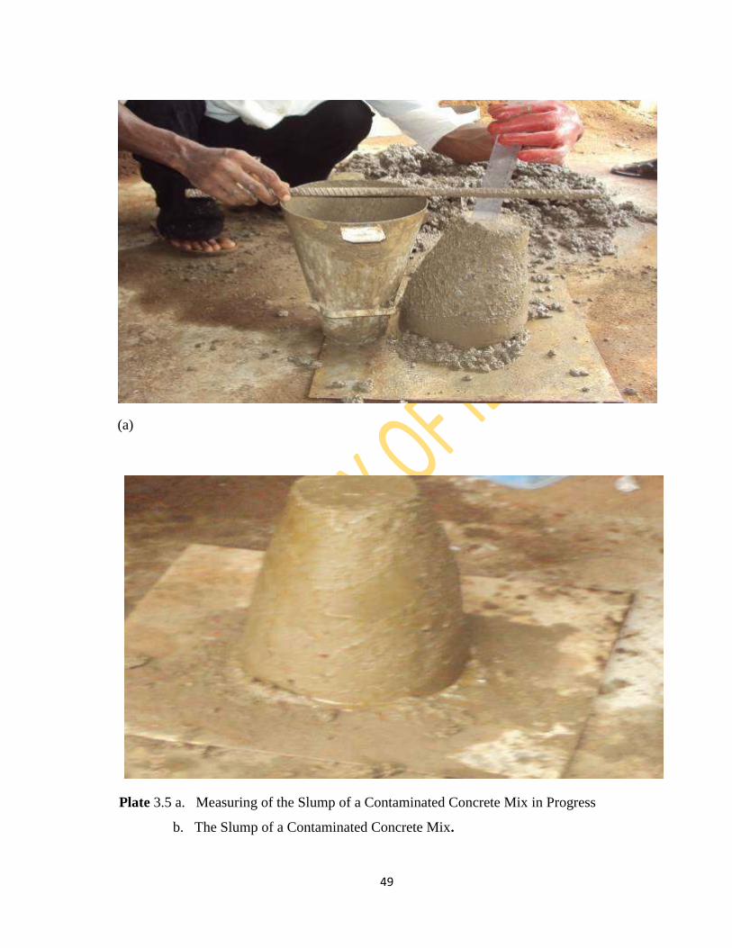
49
(a)
Plate 3.5 a. Measuring of the Slump of a Contaminated Concrete Mix in Progress
b. The Slump of a Contaminated Concrete Mix.

50
Procedure:
The cylinder was weighed empty, set in position and covered. Concrete as mixed
was put into the top hopper gently to fill approximately, but no consolidation was given. It
was then allowed to fall into the second hopper by release of the top flap. When settled in
the second hopper, the cylinder was uncovered and the second flap opened. The cylinder
fills and some concrete spills over. Consolidation is only by gravity.
The excess concrete was cut off by two trowels working inward and the full
cylinder then removed and weighed. The net weight was obtained. The cylinder was then
emptied, and refilled in layers approximately 50 mm deep and heavily rammed or
preferably vibrated (if of low workability) and completely filled. The objective was to
remove all air voids after reweighing; the second net weight was calculated.
The compacting factor was obtained as the ratio of the actual density obtained
during the test to the density of fully compacted concrete.
The compacting factor, (CF) =1st net weight/2nd net weight
This is a fraction and the higher its value the more workable; and the lower, the less
workable. Compacting factor is always less than one (BS 1881 Part 103: 1993; British
Cement Association, 1993).
3.6.1.3. Flow table test
This method gives an indication of the concrete consistency and cohesiveness and
also proneness to segregation by measuring the spread of a pile of concrete subjected to
jolting. This test is of greatest value with regard to segregation. However it gives a good
assessment of consistency of stiff, rich and cohesive concrete mixes. The flow table test
gives satisfactory results for concrete of the consistencies for which slump test may be
used.
Apparatus: The test requires two apparatuses as follows:
1. Mould: A mould in the form of a frustum of cone of base diameter 250 mm, top
diameter 170 mm and height 120 mm. The internal surface of the mould should be
smooth. It should also be provided with two handles. A tamping rod 600 mm long
and 16 mm diameter having one end rounded is also needed for rodding the
concrete.

51
2. Flow table: It is a 760 mm square brass top table. It is mounted in such a way that it
can be jolted by a drop of 13 mm. This table is bolted to a concrete or wooden base
having a height of 400 mm and weighing not less than 140 kg.
Both the flow table and the mould were fabricated purposely for this research
(Plates 3.7a and b). The test was conducted in accordance with the procedure stated in BS
1881 PT 105 (1983) for each of the contaminated mixes and the control.
Procedure:
To perform the test, the cone mould was placed at the centre of the plate and filled
in two layers, each of which was compacted with a tamping rod. The plate was lifted with
the attached handle a distance of 40 mm and then dropped a total of 15 times. The
horizontal spread of the concrete was measured. Resistance to segregation can be assessed
qualitatively: in concrete mixes that are susceptible to segregation, the paste will tend to
separate from the coarse aggregate around the perimeter of the concrete mass.
3.6.2. Tests on hardened concrete
Tests were also conducted on hardened concrete to investigate the effect of Crude
Oil Contaminated Sand on the engineering properties of concrete. Tests on hardened
concrete were categorized into two: strength tests and durability tests.
3.6.2.1. Strength tests
Compressive and flexural strength tests were conducted on contaminated samples
as well as the control samples.

52
(a)
Plate 3.6a. The Compacting Factor Apparatus Ready for Use
b. Compacting Factor Test in Progress

53
(a)
Plate 3.7a: Flow Table (Locally fabricated) Test in Progress
b. Spread of Concrete Being Measured in a Flow Table Test in Progress

54
3.6.2.1.1 Compressive strength test
The cubes produced were of size 100 mm x 100 mm x 100 mm. The filling of the
mould was in three layers and were manually compacted using 16 mm diameter metal rod
at 25 strokes per layer (BS 1881: Part 1, 1983). Following this, 147 concrete cubes
comprising of 21 controls and 126 crude oil contaminated specimens were produced. The
cubes were demoulded after 24 hrs of casting and cured in a water container (BS 1881:
Part 111, 1983). The compressive strength gained was observed at ages 3, 7, 14, 28, 56,
84, and 168 days (BS 1881-116, 1983). The compressive test was conducted at Segun-
Labiran & Associates, Consulting Civil & Structural Engineers material laboratory (Plate
3.8). The compressive strengths of the tested samples were obtained from the following
relationship:
Compressive Strength = P/A (N/mm2)
Where:
P = Ultimate compressive load on concrete (kN)
A = Surface area in contact with the platens (mm2)
3.6.2.1.2. Flexural strength (Modulus of Rupture) test
100 mm x 100 mm x 500 mm timber formwork and steel moulds were used for the
casting of both contaminated and control samples of unreinforced concrete beams. Three
specimens each were cast per percentage of crude oil contamination and control. Thus a
total of 21 beam samples (18 contaminated, 3 uncontaminated-control beams) were cast
for the experiment. The samples were cured in water, separating the contaminated samples
from the control, for 28 days after which they were weighed and tested for flexure in a
Universal Testing Machine (UTM) (Plates 3.9a and b). Single/central point loading
method of flexural test was adopted and was carried out at the material laboratory of
Polytechnic Ado-Ekiti in accordance to EN 12390-5 (2000). Both the crushing load and
the point of fracture from each support ends were determined.

55
Plate 3.8. Cube in a Compression Machine Ready for Crushing

56
The flexural strength of the resulting concrete beam using central point loading test
was determined as
Fcf = (3 x F x l)/(2xd1xd22)
Where Fcf is the flexural strength of concrete
F is the maximum crushing load on beam
l = 3d=300 mm
d1 = d2 = 100 mm
3xl/(2xd1xd22) = 3x300/(2x100
3) = 4.5x10
-4 (mm
-2)
Fcf = 4.5x10⁻⁴
F (N/mm2)
3.6.2.2. Durability tests
The ability of the COCS concrete to resist any process of deterioration-durability,
was investigated via water absorption, linear shrinkage, electrical resistivity and fire
resistance tests. The control samples were also subjected to the same tests for comparison
purpose.
3.6.2.2.1. Water absorption test
The test for water absorption of concrete was performed to determine the rate of
water absorption of a given concrete mix exposed to different environmental conditions
and draw inference from such results on the durability of the concrete mix.
The test was conducted on 21 (3 control and 18 contaminated samples), 100 mm
concrete cubes and were then subjected to the test in accordance with BS 1881 Part 122
(1983). The test was carried out at the materials laboratory of the department of Civil
Engineering, University of Ibadan.

57
Plate 3.9 a. Concrete Beams after Curing Ready for Weighing
b. Concrete Beams in Universal Machine being inspected prior to Flexural Test
(a)

58
3.6.2.2.2. Shrinkage test
Drying shrinkage is defined as the contracting of a hardened concrete mixture due
to the loss of capillary water. This shrinkage causes an increase in tensile stress, which
may lead to cracking, internal warping, and external deflection, before the concrete is
subjected to any kind of loading. The behavior of COCS concrete in relation to shrinkage
needs to be examined and thus its consideration among the tests conducted. The ASTM C
157 test for shrinkage allows the use of either 100 by 100 mm (4 inch) or 75 by 75 mm (3
inch) concrete cubes depending on the maximum aggregate size. For a maximum
aggregate size of 25 mm (1 inch), either size of concrete cubes may be used, since rate and
magnitude of shrinkage are influenced by specimen size, any specification based on
ASTM C 157 must include the specimen size. Thus 100 mm cubes were considered in this
test.
The mould preparation was done as in reference to paragraph 3.6 of ASTM C 157,
and also casting of 21 (3 control and 18 contaminated samples) 100 mm concrete cubes in
reference to paragraph 3.7 ASTM C 157. As per the code requirement, the samples were
cured in lime-saturated water for 27 days and other procedures were followed accordingly.
3.6.2.2.3. Surface resistivity indication of concrete’s ability to resist chloride ion
penetration
This non-destructive laboratory test method determines the electrical resistivity of
water-saturated concrete and provides a rapid indication of its resistance to the penetration
of chloride ions. The test result is a function of the electrical resistance of the specimen.
According to the AASHTO T XXX-08, Surface resistivity meter (0 to 100 kΩ-cm
range, resolution of 0.1 kΩ-cm and an accuracy of +/- 3% of reading) with a Wenner
linear four-probe array, was used to measure the resistivity of 200 mm nominal length and
100 mm nominal diameter cylinderical moulds meeting the requirements of ASTM C-470
were the major apparatuses used to conduct the test. A total of 21 (3 control and 18
contaminated samples) cylindrical concrete samples were cast for the test with three
samples cast for each of the percentage contamination and in accordance to ASTM C-192
or ASTM C-31. All specimens were moist cured in accordance to ASTM-192. Using the
resistivity metre locally fabricated for this research, an AC potential difference was

59
applied in the outer pins of the Wenner array generating current flow in the concrete. The
potential difference generated by this current was measured by the two inner probes. The
current used and the potential obtained along with the area affected were used to calculate
the resistivity of the concrete in Ohms-cm. Resistivity of the concrete specimens to the
flow of current were measured following the procedure stated in AASHTO T XXX-08
and the average readings for the different categories were recorded and used to
characterize the penetrability of the specimens.
3.6.2.2.4. Fire Resistance
The test was conducted on 21 (3 control and 18 contaminated samples), 100 mm
concrete cubes in accordance with IS:519-1959. The test examined the effect of elevated
temperature of 2000C on COCS concrete cubes as percentages of crude oil contamination
increases. The preparation of the mould, casting, curing and monitoring of the
compressive strength of the heated samples were as discussed under section 3.6.2.1.1.
The compressive test was conducted at SEGUN-LABIRAN & ASSOCIATES
consulting Civil & Structural Engineers material laboratory.
3.7. Experimental Control
To ensure reliability of the test results, some measures were taken to ensure that
alternatives adopted as substitutes to any of the recommended equipment or apparatus for
tests produced results similar to the expected ones assuming the appropriate specifications
were followed.
3.7.1. Casting of concrete samples:
Timber moulds were used for both concrete cubes and beams for compressive
strength and flexural strength tests respectively. This was against the recommended steel
materials in the British Standard. Thus, for the two cases, the steel moulds were used to
cast samples, three each, for cubes and beams and cured for 28 days. The compressive test
and flexural strength test were conducted on the cubes and beams respectively and
subsequently compared with that of timber mould samples.
Also, all the precautions stated along-side the different tests in the standards were
strictly adhered to during the testing operations. For slump test, the workability of a
concrete mix changes with time due to the hydration of the cement and, possibly, loss of

60
moisture. Tests on different samples were, therefore, carried out at a constant time interval
after mixing in order to obtain comparable results.
3.8. Development of Models
Statistical models were carried out to establish the influence of the percentage
crude oil contamination of sand on fresh and hardened properties of COCS concrete. Such
responses included compressive strength, flexural strength, chloride resistivity, water
absorption, slump, campacting factor, and flow. Response Surface Methodology (RSM)
was adopted in developing the models using Design Expert-8.0.5.2 software package. A
model was developed for compressive strength to allow for the variation of strength with
curing age while other models were developed to predict other parameters. The design
summary for compressive strength model and models for others are as stated in sections
3.8.1 and 3.8.2 respectively.
3.8.1. Design summary for compressive strength model
The design parameters for modelling compressive strength are as stated below.
Similarly the experimental factor input and measured response input for compressive
strength model development are presented in Tables 3.2 and 3.3 respectively.
Study Type Response Surface Runs 49
Design Type Central Composite Blocks No Blocks
Design Model Quadratic Build Time (ms) 4.45
Factor A: Crude Oil Contamination (%) Factor B: Curing Age (Days)
3.8.2. Design summary for other properties
Similarly, the experimental factors input and measured responses input of other
properties‘ model development are presented in Tables 3.4 and 3.5 respectively.

61
Table 3.2. Experimental Factor Input for Compressive Strength
Factor Type Sub-Type Actual Value Coded Value
Mean Standard
Deviation
Min. Max. Min. Max.
A Numeric Continuous 0.00 25.00 -1.00 1.00 11.07 8.65
B Numeric Continuous 3.00 168.00 -1.00 1.00 51.43 54.69

62
Table 3.3. Measured Response Input for Compressive Strength
Resp-
onse Name Units Obs
Analy-
sis Min. Max Mean
Std.
Dev. Ratio Trans. Model
Y1 Compr.
Strength N/mm
2 49
Poly
nomial 0.83 40.3 13.86 10.37 48.55 Log10 Sixth

63
Table 3.4. Experimental Factor Input for Other Properties
Resp-
onse Name Units Type
Sub-
type
Actual
Values
Coded
Values Mean
Std.
Dev. Min Max Min Max
A Crude
Oil % Numeric Cont. 0.00 25.00 -1.00 1.00 10.11 9.52
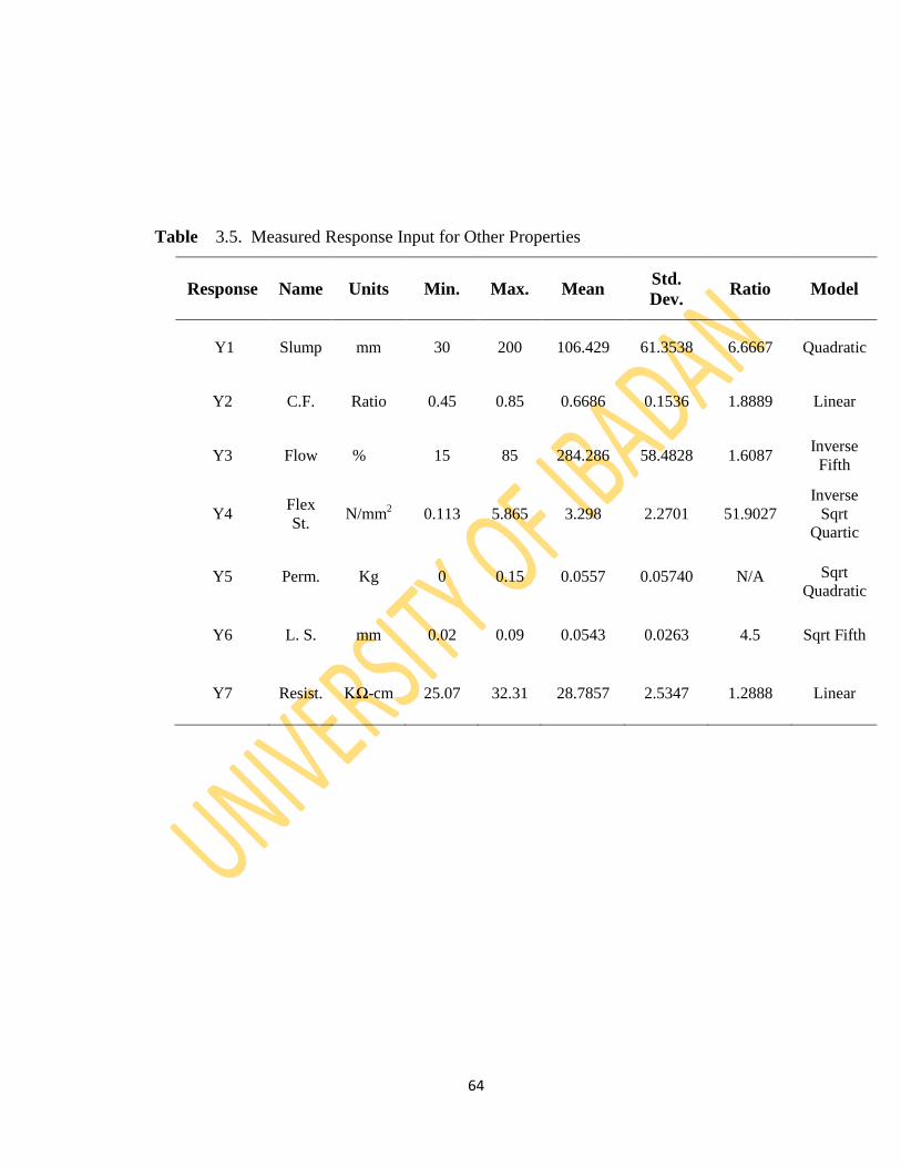
64
Table 3.5. Measured Response Input for Other Properties
Response Name Units Min. Max. Mean Std.
Dev. Ratio Model
Y1 Slump mm 30 200 106.429 61.3538 6.6667 Quadratic
Y2 C.F. Ratio 0.45 0.85 0.6686 0.1536 1.8889 Linear
Y3 Flow % 15 85 284.286 58.4828 1.6087 Inverse
Fifth
Y4 Flex
St. N/mm
2 0.113 5.865 3.298 2.2701 51.9027
Inverse
Sqrt
Quartic
Y5 Perm. Kg 0 0.15 0.0557 0.05740 N/A Sqrt
Quadratic
Y6 L. S. mm 0.02 0.09 0.0543 0.0263 4.5 Sqrt Fifth
Y7 Resist. KΩ-cm 25.07 32.31 28.7857 2.5347 1.2888 Linear

65
3.9. Mix Proportioning for Enhanced Strength COCS Concrete
The purpose of mix proportioning is to obtain a product that will perform
according to certain predetermined requirements (Hansen and Demaro, 1997), the most
essential requirements being the workability of fresh concrete and the strength and
durability of the hardened concrete. This exercise followed the outcome of the
investigation of the effect of COCS on the fresh and hardened properties of concrete. The
concrete constituents were re-proportioned using the COCS (5 and 10% contaminations)
with the aim of finding an appropriate mix that would produce desired compressive
strength relative to that of uncontaminated concrete. The water cement ratio was reduced
from 0.5, used for the previous experiment, to 0.45, 0.42, 0.38, and 0.35. For the sake of
workability, a super plasticizer – CONPLAST-SP 430, was added to mixes of w/c of 0.38
and 0.35. The four different mixes were designed using British method-DOE (See section
3.4.1 of this thesis) and the material proportion schedule is presented in Table 3.6. A total
of 108 (12 controls and 96 contaminated samples with varying w/cs) samples, 100 x 100 x
100 mm cubes were cast and cured for ages 3, 7, 14, and 28 days. The compressive
strength of the cubes were determined at the curing ages.

66
Table 3.6. Mix Proportion of Materials
Water/
Cement
Ratio
Material Quantities (Kg/m3)
Plasticizer
(L/ m3)
Plastic
Density
(Kg/m3)
Cement Sand Granite Water
0.5 400 720 1080 200 - 2400
0.45 444 710 1066 200 - 2420
0.42 488 686 1031 205 - 2410
0.38 500 690 1050 190 7.50 2430
0.35 500 710 1065 175 10.00 2450

67
CHAPTER FOUR
RESULTS AND DISCUSSION
4.1. Results of Preliminary Studies
4.1.1. Sieve analysis
The results of particle size grading of the contaminated samples, and the
uncontaminated fine and coarse aggregates are presented in Figs. 4.1 to 4.5. The grading
curves of all the fine aggregate samples fell within the fine aggregate grading envelope as
specified in BS 812: Part 103 (1989). From the particle size distribution curve of the
uncontaminated fine aggregate (Fig. 4.4), it was deduced that the fine aggregate consist of
12% fine, 65% medium and 23% coarse sand. It possesses coefficient of uniformity (Cu)
of 4.3 and coefficient of curvature (Cc) of 0.74 which shows that the fine aggregate is well
graded.
The coarse aggregate when analysed had more than 80% of its particle fell within
13.2 mm and 6.7 mm sieve sizes. This conformed to the specification by BS 1881 PT 108
(1983) that for a cube size of 100 x 100 x 100 mm, the nominal size of aggregate must not
exceed 20 mm. Also, Fig. 4.5 shows that the coarse aggregate is of the normal size of
graded aggregate based on BS 812: Part 103 specification. This can be used for normal
concrete works.
4.1.2. Result of Total Petroleum Hydrocarbon (TPH)
The results of TPH analysis of the soil samples obtained from the three polluted
sites are presented in Table 4.1 below. The results showed that samples from B-Dere have
the highest average percentage crude oil contamination of 14.1%, Bodo has 10.1%
contamination while Bomu has lowest value of 8.6%. Based on this result, the percentage
contamination by weight of sand for the research was set at 2.5%, 5.0%, 10.0%, 15.0%,
20.0%, and 25.0%.

68
Fig. 4.1. Particle Size Distribution Curve of Sand from Bodo Spill Location.
Sieve Metric Size (mm)
Per
cen
tage
Pass
ing (
%)

69
Fig. 4.2. Particle Size Distribution Curve of Sand from Bomu Spill Location.
Sieve Metric Size (mm)
Per
cen
tage
Pass
ing (
%)

70
Fig. 4.3: Particle Size Distribution Curve of Sand from B-Dere Spill
Location
Per
cen
tage
Pass
ing (
%)
Sieve Metric Size (mm)
Fig. 4.3. Particle Size Distribution Curve of Sand from B-Dere Spill Location.

71
Weight of Soil Sample = 500g
Sieve Metric Size (mm)
Fig. 4.4. Particle Size Distribution Curve of Uncontaminated Fine Aggregate

72
Sieve Metric Size (mm)
Per
cen
tage
Pass
ing (
%)
Fig. 4.5: Particle Size Distribution Curve of Coarse Aggregate

73
Table 4.1. TPH Test Results
S/N Sample
Location
ID/Code TPH (%) AVG (%)
1
B-DERE
CS1A 15.4
14.1±1.30 2 CS1B 12.8
3 CS 1C 14.1
4
BOMU
CS 2A 8.43
8.6±0.15 5 CS 2B 8.68
6 CS 2C 8.69
7
BODO
CS 3A 10.23
10.1±0.14 8 CS 3B 9.96
9 CS 3C 10.11

74
4.2. Results and Discussions of Tests on Concrete Samples
The results of the different tests conducted on both fresh and hardened concrete to
investigate the effect of crude oil contaminated sand on the properties of concrete are as
presented in the following sections. Similarly, the corresponding impacts of COCS, based
on the test results, on concrete are inferred.
4.2.1. Results of tests on fresh concrete
4.2.1.1. Slump test
The slump values obtained for each of the samples are as presented in Table 4.2
below. When compared with the control sample‘s slump value of 30, the contaminated
samples have greater values that increase with increase in percentage contamination of
sand with crude oil. The slump value increases from 55 for 2.5% contamination to 200 for
25%. This implies that the addition of crude oil to sand will improve the workability of
concrete, the slump values corresponding to medium-high workability levels. It is,
however, obvious that increasing crude oil contamination beyond 25% will further
increase the slump till it ultimately become too wet and thus result into a collapse slump.
4.2.1.2. Compacting factor test
Though the test is more suitable for low workability concrete having a slump of
less than 10, applying the test to the samples further revealed that COCS concrete samples
have higher compacting factor and thus higher workability when compared with the
control sample. The compacting factors of the contaminated samples increased with
increase percentage contamination (Table 4.3). The very low workability implied by the
results is due to the fact that the samples are not of the dry mix for which the test is most
suitable.
4.2.1.3. Result of Flow Table test
The flow test is most suitable for very high workability concrete with a slump of
more than 175, applying the test to all the samples, however, clearly established that the
presence of crude oil in the mix truly improves the workability. While the flow rate of the
control mix was 15% (Table 4.4), a contamination of 2.5% crude oil in sand increased the
flow rate by 3% and this trend increases as the crude oil percentage increases. Hence, 25%

75
Table 4.2. Results of Slump Test
Crude oil
Contamination (%) Slump (mm) Degree of workability
0 30 Low
2.5 55 Medium
5.0 75 Medium
10.0 95 Medium
15.0 120 High
20.0 170 High
25.0 200 High

76
Table 4.3. Results of Compacting Factor Test
Crude Oil
Contamination
(%)
Compacting
Factor Remark
0 0.45 Very Low
2.5 0.48 Very Low
5.0 0.65 Very Low
10.0 0.70 Very Low
15.0 0.75 Very Low
20.0 0.80 Very Low
25.0 0.85 Low
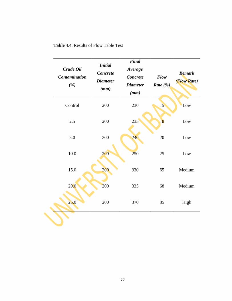
77
Table 4.4. Results of Flow Table Test
Crude Oil
Contamination
(%)
Initial
Concrete
Diameter
(mm)
Final
Average
Concrete
Diameter
(mm)
Flow
Rate (%)
Remark
(Flow Rate)
Control 200 230 15 Low
2.5 200 235 18 Low
5.0 200 240 20 Low
10.0 200 250 25 Low
15.0 200 330 65 Medium
20.0 200 335 68 Medium
25.0 200 370 85 High

78
contamination produced a flow rate of 85%, a value far more than that of the control
value.
4.2.2. Effect of COCS on the fresh properties of concrete
Fresh concrete is defined as workable and consistent when the concrete can be
transported, placed, compacted and finished sufficiently easily and without segregation.
When the sand with different percentages of crude oil contamination were mixed to
produce the contaminated concrete samples, the property at the concrete fresh state differ
from the control sample. The three tests conducted on the concrete samples at the fresh
state established that COCS concrete is more workable than the uncontaminated mix. The
presence of crude oil in the mix acted as a plasticizer improving the fluidity and almost
doubling the slump of the concrete mix at 2.5% contamination. Also, crude oil plasticize
fresh concrete mixtures by reducing the surface tension of water and thus reduces the
quantity of water required for cement hydration. This implies that COCS concrete is more
easily transported, placed and compacted when compared with the uncontaminated
concrete.
4.3. Results and Discussions of Tests on Hardened Concrete
4.3.1. Strength test results
4.3.1.1. Compressive strength test results
The results of the compressive strength test are depicted in Fig. 4.6 (see details in
Appendix A.). The compressive strength for all the samples increased with time but at
different rate. The control sample maintains the highest compressive strength values over
time while the values for the contaminated samples decreased with increase in crude oil
contamination but increases with time. The percentage reduction in compressive strength
of COCS concrete in relation to the control is expressed graphically in Fig. 4.6 to show the
level of strength loss. The average of the percentage strength reduction indicated that
about 18% of the strength was lost when the soil was contaminated with 2.5% crude oil
while almost 90% of the strength was lost due to 25% contamination (Fig. 4.7).

79
Fig. 4.6: Compressive Strength Development of Concrete
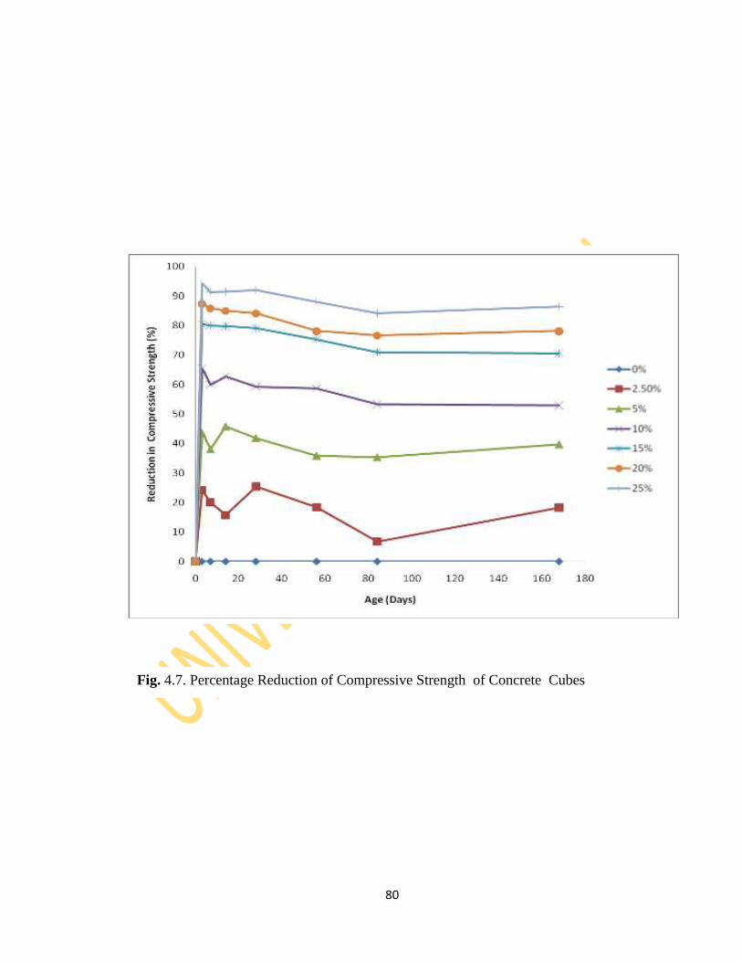
80
Fig. 4.7. Percentage Reduction of Compressive Strength of Concrete Cubes

81
4.3.1.2 Flexural strength test results
The results of the flexural strength tests (Table 4.5) indicated a negative effect of
COCS on the flexural strength of concrete. The results are similar to that of the
compressive strength in that the flexural strength reduces with increase in crude oil
percentage contamination. Thus the control sample had the highest value of 5.87 N/mm2
while the highest percentage contamination gave the lowest value of 0.11 N/mm2. The
presence of crude oil in the sand of concrete will reduce its flexural strength.
4.3.2 Effect of COCS on the Strength of Concrete
The effect of COCS was negative on both the compressive and flexural strengths
of concrete. The values of the control maintained a consistent increase in compressive
strength as the curing age increases. This is not surprising as the strength of cement-based
materials cured in water with no contamination increases with age. The crude oil
contaminated concrete cubes also increases but at lower rate of strength development. The
reduction in strength can be related to the varying percentages of crude oil contamination
in the concrete which may lead to loss of water content/moisture and preventing water
from entering the concrete cube when curing in water which has effect on the hydration of
cement present in the concrete cubes. The contamination of fine aggregate with crude oil
which forms part of the microstructure of the matrix of concrete may have caused dilation
of the gel and weakening of the cohesive forces in the paste and hence low strength
development of the concrete cubes cast with COCS. The outcome of this research as per
compressive strength reduction is in agreement with the findings of past researchers
(Onabolu, 1989; Ramzi, 2000; Ejeh and Uche, 2009); on the adverse effect of
hydrocarbons on concrete.
The large losses in compressive strength imply that crude oil percentages above
10% would not be suitable for most structural applications where high compressive
strengths are required (Ajagbe et al., 2011). However, this type of concrete could be used
in low-strength-concrete applications e.g. sidewalks, sandcrete blocks, etc. Due to the low
strength of COCS concrete which would not be acceptable for reinforced concrete in most
cases, the research was thereafter extended to improve on the strengths of 5% and 10%

82
contaminated COCS concrete by reducing the water cement ratio and the addition of
plasticizer to assist the concrete in workability at low water/cement ratio.
4.3.3 Durability test results
4.3.3.1. Water absorption test result
The water absorption characteristic of the COCS concrete is as shown in Table 4.6.
The increase in the dimensions and weight of the samples clearly showed that water was
absorbed by the concrete samples but in varying quantity. While the control sample
absorbed the highest volume of water, the quantity of water absorbed by COCS concrete
samples reduced as the percentage of crude oil increases and this implies that COCS
concrete offer resistance to the penetration of water. The outcome of the tests is better
explained by the fact that water and oil are immiscible and thus the presence of crude oil
in the concrete repels water and thus prevented it from penetrating. In porous solids, water
is known to be the cause of many types of physical processes of degradation and as a
vehicle for transport of aggressive ions; water can also be a source of chemical processes
of degradation. Also, the physical-chemical phenomena associated with water transport in
porous solids are controlled by the permeability of the solid (Mehta and Monteiro, 2006).
This behavior of COCS concrete makes it more durable than the uncontaminated concrete
since there would be resistance to aggressive chemicals or elements, such as chloride,
from penetrating into the concrete thus protecting the reinforcement in reinforced concrete
from corrosion.
4.3.3.2 Shrinkage test results
With reference to Table 4.7, the linear shrinkage of the sample was much on the
control when compared with contaminated samples. The 25% crude oil contamination was
least affected by shrinkage. Shrinkage is one of the detrimental properties of concrete,
which affects its long-term strength and durability. Volume change in concrete results into
the formation of unsightly cracks and is one of the most objectionable defects particularly
in floors and pavements. Shrinkage particularly contributes to the formation crack.
Therefore, the presence of crude oil in the fine aggregate of the concrete has limited its

83
Table 4.5. Flexural Strength Test Results
Contamination
(%)
Avg. Weight
(kg)
Flexural
Strength
(N/mm2)
0 11.97 5.87
2.5 11.87 4.82
5.0 10.98 4.70
10.0 11.73 4.53
15.0 11.55 2.57
20.0 11.57 0.50
25.0 11.51 0.11

84
Table 4.6. Water Absorption Test Result
Crude oil
Contamination
(%)
Change in Dimension (∆L) in cm Weight
Difference
(Kg) Length Breadth Depth
0 0.13 0.12 0.12 0.15
2.5 0.10 0.08 0.08 0.12
5 0.06 0.05 0.05 0.05
10 0.04 0.04 0.04 0.04
15 0.03 0.03 0.03 0.02
20 0.01 0.02 0.02 0.01
25 0.00 0.01 0.01 0.00

85
Table 4.7. Shrinkage Test Results
Crude oil
Contamination
(%)
Change in Dimension (∆L) in cm
Length Breadth Depth
0 0.10 0.08 0.09
2.5 0.08 0.07 0.08
5 0.07 0.06 0.07
10 0.05 0.05 0.06
15 0.04 0.04 0.05
20 0.03 0.03 0.03
25 0.01 0.02 0.02

86
volume change and hence the shrinkage. It could be said that COCS concrete is more
durable than uncontaminated concrete when subjected to similar conditions of shrinkage.
4.3.3.3 Concrete Electrical Resistivity test results
Likewise, the same observation was made for the concrete electrical resistivity test
as a rapid indication of its resistance to the penetration of chloride ions. The control mix
of concrete cylinders made with uncontaminated sand offered least resistance to the
passage of electric current ranging from about 24.00 to 25.50 KΩ-cm, which can be
compared with International Standard Surface Resistivity Penetrability (Table 4.8). The
control mix of concrete cylinder made with uncontaminated sand show a trend of about 21
– 37 KΩ-cm, indicating a low chloride ion penetrability. Similarly, the contaminated
samples displayed lower chloride penetration when compared with the control. The
chloride ion penetrability reduces with increase in crude oil percentage contamination
(Table 4.9).
4.3.3.4 Fire Resistance test result
The compressive strength of sample cubes subjected to elevated temperature of
200ºC was used as an indication of the fire resistance of the samples. Significant decrease
in compressive strength of heated concrete cubes were observed with increased in
percentage contamination. The compressive strength decreased from 21.2 N/mm2 (control)
to 3.33 N/mm2 for 15% contamination (See Table 4.10) . By these results, fire resistance
of concrete decreases as the crude oil contamination level in the fine aggregate increases.
This is not unconnected with the fact that crude oil is a fuel that can on its own aid
ignition of fire. It specifically increases the heat within the concrete which resulted into
the reduction of the concrete strength.

87
Table 4.8. Chloride Ion Penetrability Based
Chloride Ion
Penetrability
Surface Resistivity Test
100 mm X 200 mm
Cylinder (KΩ-cm) a = 1.5
150 mm X 300 mm
Cylinder (KΩ-cm) a = 1.5
High < 12 < 9.5
Moderate 12 -21 9.5 – 16.5
Low 21 – 37 16.5 – 29
Very Low 37 – 254 29 – 199
Negligible ˃254 ˃199
a = Wenner probe tip spacing
AASHTO: T XXX-08

88
Table 4.9. Concrete Surface Resistivity Test Results
Crude oil Contamination
(%)
Surface Resistivity Test
(KΩ-cm)
Chloride Ion
Penetrability
0 25.07 Low
2.5 27.22 Low
5.0 28.05 Low
10.0 28.38 Low
15.0 28.66 Low
20.0 31.81 Low
25.0 32.31 Low

89
Table 4.10. Compressive Strength of Heated (200˚C) COCS Concrete Cubes
Crude oil
Contamination
(%)
Specimen Crushing
Load (N)
Compressive
Strength
(N/mm2)
Average Compressive
Strength (N/mm2)
0.0
A1 215 21.5
21.17±1.04 A2 220 22.0
A3 200 20.0
2.5
B1 170 17.0
17.33±0.29 B2 175 17.5
B3 175 17.5
5.0
C1 138 13.8
13.77±0.25 C2 140 14.0
C3 135 13.5
10.0
D1 100 10.0
11.17±1.26 D2 125 12.5
D3 110 11.0
15.0 E1 35 3.5 3.33±0.29
E2 35 3.5
E3 30 3.0
20.0 F1 29.1 2.9 2.7±0.34
F2 28.9 2.9
F3 23.3 2.3
25.0 G1 12.1 1.2 1.1±0.10
G2 1.05 1.1
G3 1.04 1.0

90
4.3.4 Effect of COCS on the durability of concrete
Unlike the effect of COCS on the strength of hardened concrete, the durability
tests conducted in this research showed clearly that the effect of crude oil in the sand of
the concrete improves the resistance of the COCS concrete to water and chloride
penetrability. These two attributes greatly increases the durability of the concrete by
preventing the corrosion of steel and other substances that may affect the durability of
concrete. The use of COCS concrete can thus be extended to the production of concrete
products wherein the absorption of water affects the aesthetics as is the case in roof tiles,
and reduces the passage of water in liquid retainning structures such as septic tank etc. In
addition, the reduction of water absorption by COCS concrete makes it a better choice as
damp proof courses in a water logged area to reduce seepage.
The low fire resistance of the COCS concrete will not compromise the durability
of the concrete when adopted in the liquid retainning structures and damp proof courses as
suggested above. Furthermore, the exhibition of good durability properties by the COCS
confirmed the recommendations by Al-Mutairi and Eid (1997) of the suitability of the
material for use in the production of asphalt concrete mixes for use in secondary roads,
road beds, impermeable layers for landfill and containment facilities, or as stabilizers for
steep embarkments.
4.4 Mathematical Models
The result of the derived models in this research is presented, along with the
correlation coefficients and the relative significance.
4.4.1. Compressive strength model
The response surface methodology was used to investigate the effect of some
parameters (crude oil contamination and curing age) on the compressive strength of
concrete. The experimental values for compressive strength at 3, 7, 14, 28, 56, 84 and 168
days under different crude oil contamination percentages are presented in Table 4.11 . The
model summary statistics of linear, 2FI (Two Factors Interaction), quadratic, cubic,
quartic, fifth and sixth polynomials are presented in Table 4.12. Statistical analysis for
compressive strength at the curing ages and different contamination percentages indicated
that the model (sixth order polynomial) with coefficient of correlation R2 equal to 0.9982

91
was adequate, possessing less significant lack of fit than other models and its thus the best
one fit. The final model, after a base 10 logarithmic transformation, for the compressive
strength as determined by the above analysis is presented below.
Log10(Compressive Strength) = 0.73288+9.07341E-003*A+0.14930*B-0.030193*A2-
0.013114*B2+6.07861E-003*A
3+5.28517E-004*B
3-5.35718E-004*A
4-9.78501E-
006*B4+2.130221E-005*A
5+9.97399E-007*B
5-3.11650E-007*A
6-2.24025E-
010*B6 ...(Eqtn. 4.1)
Fig. 4.9 show the correlation between measured and predicted models while Fig.
4.10 shows the non-linear response surface interactions between the factors.
4.4.2. Models for other properties
The input parameters and the model types for the slump, compacting factor, flow,
flexural strength, permeability, linear shrinkage and chloride resistivity of the COCS
concrete are shown in Table 4.13. Similarly, the model equations and the R2 values for
each of the responses are presented in Table 4.14. Statistical analysis for slump and
compacting factor was best described by linear type model while a model based on the
inverse of flow values gave a R2 of 1.000. Linear model also described permeability and
resistivity better while a transformation of the inverse of the square root of flexural
strength improved the R2 to 0.9950.
Based on the correlation observed between the measured and the predicted models
for all the factors, the models can be used to navigate the design space. Thus the fresh and
hardened properties of concrete when made with COCS can be predicted by the developed
models. Further details on the statistical analyses of the models are contained in appendix
B.

92
Table 4.11. Input Details Showing Factors and Response
Order
Factor A:
Contamination
(%)
Factor B:
Curing Age
(Days)
Response 1:
Compressive Strength
(N/mm2)
1 0.00 3.00 14.50
2 0.00 7.00 21.25
3 0.00 14.00 25.50
4 0.00 28.00 31.50
5 0.00 56.00 33.50
6 0.00 84.00 33.50
7 0.00 168.00 40.30
8 2.50 3.00 11.00
9 2.50 7.00 17.00
10 2.50 14.00 21.50
11 2.50 28.00 23.17
12 2.50 56.00 27.33
13 2.50 84.00 31.25
14 2.50 168.00 33.00
15 5.00 3.00 8.17
16 5.00 7.00 13.17
17 5.00 14.00 13.83
18 5.00 28.00 18.33
19 5.00 56.00 21.50
20 5.00 84.00 21.67
21 5.00 168.00 24.30
22 10.00 3.00 5.00
23 10.00 7.00 8.50
24 10.00 14.00 9.50
25 10.00 28.00 12.83
26 10.00 56.00 13.83

93
Table 4.11. Input details Showing Factors and Response (Cont‘d).
Order
Factor A:
Contamination
(%)
Factor B:
Curing Age
(Days)
Response 1:
Compressive
Strength
(N/mm2)
27 10.00 84.00 15.67
28 10.00 168.00 19.00
29 15.00 3.00 2.83
30 15.00 7.00 4.25
31 15.00 14.00 5.17
32 15.00 28.00 6.61
33 15.00 56.00 8.27
34 15.00 84.00 9.73
35 15.00 168.00 11.90
36 20.00 3.00 1.83
37 20.00 7.00 3.00
38 20.00 14.00 3.83
39 20.00 28.00 5.00
40 20.00 56.00 7.33
41 20.00 84.00 7.83
42 20.00 168.00 8.80
43 25.00 3.00 0.83
44 25.00 7.00 1.83
45 25.00 14.00 2.17
46 25.00 28.00 3.50
47 25.00 56.00 4.00
48 25.00 84.00 5.33
49 25.00 168.00 5.50

94
Table 4.12. Model Summary Statistics
Source Std. Dev. R-Squared Adjusted
R-Squared
Predicted
R-Squared
PRESS
Linear 0.13 0.8947 0.8902 0.8788 0.91
2FI 0.13 0.9031 0.8966 0.8800 0.90
Quadratic 0.087 0.9565 0.9514 0.9421 0.44
Cubic 0.063 0.9793 0.9745 0.9664 0.25
Quartic 0.051 0.9881 0.9833 0.9758 0.18
Fifth 0.043 0.9930 0.9880 0.9723 0.21
Sixth 0.026 0.9982 0.9959 0.9764 0.18 Suggested
Response 1: Compressive Strength Transform: Base 10 Log Constant: 0

95
Fig. 4.9. Comprssive Strength Measured Values Vs Predicted Values
Design-Expert® SoftwareCompressive Strength
Color points by value ofCompressive Strength:
40.3
0.83
Actual
Pre
dic
ted
Predicted vs. Actual
0.00
10.00
20.00
30.00
40.00
50.00
0.00 10.00 20.00 30.00 40.00 50.00

96
Fig. 4.10. Response Surface for Desirability Effects of Variables Interactions
Design-Expert® SoftwareFactor Coding: ActualOriginal ScaleCompressive Strength
Design points above predicted valueDesign points below predicted value40.3
0.83
X1 = A: ContaminationX2 = B: Days
3.00
36.00
69.00
102.00
135.00
168.00
0.00
5.00
10.00
15.00
20.00
25.00
0.794103
4.30555E+061
8.6111E+061
1.29167E+062
1.72222E+062
C
om
pre
ss
ive
Str
en
gth
A: Contamination B: Days

97
Table 4.13. Input Parameters for the Responses and the Model Type
Response Name Units Min. Max. Mean Std.
Dev. Ratio Model
Y1 Slump mm 30 200 106.429 61.3538 6.6667 Quadratic
Y2 C.F. Ratio 0.45 0.85 0.6686 0.1536 1.8889 Linear
Y3 Flow mm 230 370 284.286 58.4828 1.6087 Inverse
Fifth
Y4 Flex
St. N/mm
2 0.113 5.865 3.298 2.2701 51.9027
Inverse
Sqrt
Quartic
Y5 Perm. Kg 0 0.15 0.0557 0.05740 N/A Sqrt
Quadratic
Y6 L. S. mm 0.02 0.09 0.0543 0.0263 4.5 Sqrt Fifth
Y7 Resist. 25.07 32.31 28.7857 2.5347 1.2888 Linear

98
Table 4.14. Statistical Models for Other Responses
Response Model Equation R2
Slump Y1 = 51.73293+3.36976A+0.10685A2 0.9535
C.F. Y2 = 0.53075+0.013626A 0.8323
Flow 1/Y3 = 4.34772E-003-4.04052E-004A+1.45468E-
004A2-1.80853E-005A
3+8.63682E-007A
4-1.40548E-
008A5
1.000
Flexural
Strength
1/√Y4 = 0.41581+0.11320A+0.021411A2+1.20874E-
003 A3-1.47846E-005 A
4
0.995
Permeability √Y5 = 0.32287-0.011316A-4.45260E-005 A2 0.8721
Linear
Shrinkage
√Y6 = 0.3003-0.072901A+0.016220 A2
-1.45447E-003
A3+5.65235E-005 A
4-8.01463E-007 A
5
1.000
Resistivity Y7 = 26.52368+0.22365A 0.8230

99
4.5. Mix Proportioning Compressive Strength Test Result
Compressive strength test for the four different mixes with COCS was carried out
at 3, 7, 14 and 28 days with the intention of improving the compressive strength of COCS
concrete when the contamination by crude oil does not exceed 10%. The results of the test
are presented in Table 4.15. It was observed from the result that the compressive strength
of the mixes increases with decrease in water cement ratio. Thus the maximum values at
28 days for 5% and 10% contamination for 0.35 water/cement ratio are 28.33 N/mm2
and
26.77 N/mm2
respectively. The designed mix ratios and the corresponding 28 days
compressive strengths are shown in Table 4.16. The least 28 days strength for 10%
contamination was 21 N/mm2 obtained at water/cement ratio of 0.45. Thus a mix ratio of
1: 1.6 : 2.4 at 0.45 water/cement ratio could be used for reinforced concrete to resist
tension provided the crude oil contamination does not exceed 10% by weight of the fine
aggregate.

100
Table 4.15. Compressive Strength for Different Mix Proportions
Crude Oil
Contamination
(%)
Water/Cement
Ratio
Compressive Strength (N/mm2)
3 Days 7 Days 14 Days 28 Days
5
0.5* 8.17 13.17 13.83 18.33
0.45 10.67 15.67 20.67 23.67
0.42 11.69 16.67 23.00 25.67
0.38 14.00 23.50 24.00 27.33
0.35 18.00 21.33 25.33 28.33
10
0.5* 5.00 8.50 9.50 12.83
0.45 10.33 15.00 19.00 21.00
0.42 11.67 16.00 22.33 23.67
0.38 13.50 18.33 22.67 25.00
0.35 13.50 19.67 24.33 26.67
*From previous experiment

101
Table 4.16. Designed Mix Ratios and their 28 days Compressive Strength
S/N Design Mix Ratio W/C
Ratio
Compressive Strength (N/mm2)
@ 28 days
5% 10%
1 1 : 1.8 : 2.7 0.5 18.33 12.83
2 1 : 1.6 : 2.4 0.45 23.67 21.00
3 1 : 1.4 : 2.1 0.42 25.67 23.67
4* 1 : 1.38 : 2.1 0.38 27.33 25.00
5* 1 : 1.42 : 2.13 0.35 28.33 26.67
*CONPLAST SP-430 -Super plasticizer added.

102
CHAPTER FIVE
CONCLUSIONS AND RECOMMENDATIONS
5.1 Conclusions
The effect of Crude Oil Contaminated Sand on the fresh and hardened concrete
was investigated in this research. The consistency and workability of COCS concrete were
evaluated through slump, compacting factor and flow table tests while the hardened
properties were estimated by assessing the compressive and flexural strengths; water
absorption, linear shrinkage, electrical resistivity and fire resistance tests. The findings of
the research are stated below:
(i). The presence of crude oil in the fine aggregate of concrete improved the
rheological behaviour of the concrete thus making the concrete more
workable. It was confirmed that hydrocarbons adversely affect the hydration
of fresh concrete and thus retard the strength gain.
(ii). The compressive strength of the COCS concrete was reduced beyond 50%
when the fine aggregate was contaminated by crude oil to more than 10% by
weight of the sand. The flexural strength of the COCS concrete was greatly
affected particularly at 20% to 25% contamination.
(iii). COCS concrete exhibited better resistance to water and chloride penetration
when compared to the uncontaminated concrete. Similarly, the COCS
concrete shrink less compared to the control sample.
(iv). COCS concrete exhibited poor fire resistance relative to the uncontaminated
concrete. The COCS concrete is suitable for use in low strength structures or
generally where durability requirement outweighed that of strength.
(v). Mathematical models were developed for compressive strength and other
properties (flexural strength, slump, compacting factor, flow, water
absorption, chloride resistivity, and linear shrinkage) of COCS concrete at 0.5
water/cement ratio.
(vi). At 0.45 water/cement ratio, a strength of 21 N/mm2
was obtained at 10%
crude oil contamination. This is a suitable strength for reinforced concrete
structures. Further reduction in water/cement ratio will increase the strength

103
accordingly, a table of compressive strength at 3, 7, 14 and 28 days for
different mix proportions was provided.
5.2 Recommendation for further Studies
Further studies in the following areas would improve the use of contaminated soils
in the polluted sites in the Niger Delta area
a. A research should be conducted on the use of COCS for sandcrete block
production.
b. More durability tests should be conducted on the COCS concrete over a longer
period of time than considered in this research.
c. The possibility of using locally available material as admixture such as
metakaolin, to improve the strength of the COCS concrete should be
investigated.

104
REFERENCES
ACI Committee, 2003. Guide for the silica fume in concrete. ACI Manual of Concrete
Practices, l. 96, 234 R-1 to 46.
ACI 1990. Cement and concrete terminology. ACI 116R-90. American Concrete Institute,
Detroit, USA.
ACI Committee 201, 2002. Guide to durable concrete. ACI Manual of Concrete Practice,
Detroit, USA.
ACI Committee 211, 2002. Guide for proportioning low slump concrete. ACI Manual of
Concrete Practice, Detroit, USA.
Agbede O. A. 1996. Ground water modelling-an overview. Journal of Mining and
Geology. 32. 2: 105-112.
Ajagbe W. O., Omokehinde S. O., Agbede O. A., and Alade G. A. 2011. Effect of crude
oil impacted sand on compressive strength of concrete. Construction and Building
Materials 26. 1: 9-12.
Alexander, K. M. 1983. A study of concrete strength and mode of fracture in terms of
matrix, bond and aggregate strengths. Tewksbury Symposium on Fracture,
University of Melbourne, 25-34.
Al-Mutairi, N. M. 1995. Kuwait oil-based pollution: effect on building material. Journal
of Materials in Civil Engineering 7. 3: 154 – 160.
Al-Mutairi, N. M. and Eid, W. K. 1997. Utilization of oil-contaminated sands in asphalt
concrete for secondary roads. Materials and structures. 30: 497-505.
Al Qadi, A. N. S., Nasharuddin, K., Al-Mattarneh, H and AL-Kadi, Q. N. S.. 2009.
Statistical Models for Hardened Properties of Self-Compacting Concrete.
American J. of Engineering and Applied Sciences 2 (4): 764-770
ASTM 1993. Standard definitions and terms relating to concrete and concrete aggregates.
American Society for Testing and Materials, West Conshohocken, Pennsylvania,
USA.
ASTM C125-93. American Society for Testing and Materials, West Conshohocken,
Pennsylvania, USA.
ASTM C143-78, Test for slump of Portland Cement Concrete. American Society for
Testing and Materials, West Conshohocken, Pennsylvania, USA.

105
Ayininuola, G. M. 2009. Influence of diesel oil and bitumen on compressive strength of
concrete. Journal of Civil Engineering (IEB), 37(1) 65-7.1
Badejo, O.T. and Nwilo, P.C. 2004. Management of oil spill dispersal along the Nigerian
coastal areas, Department of Surveying and Geoinformatics, University of Lagos.
pp. 1
Biczok, I. 1964. Concrete corrosion and concrete protection. Publishing House of the
Hungarian Academy of Sciences, Budapest. In. Wilson, S.A., Langdon, N.J. &
Walden, P.J. 2001. The effects of hydrocarbon contamination on concrete strength.
Proceedings of the Institution of Civil Engineers. Geotechnical Engineering. 149.
3:189–193.
Blaszczynski, T. Z. 2002. Reinforced concrete structures in crude oil products
environment. Proceedings of the Foundations of Civil and Structural Engineering,
Poznan University of Technology. 2.
Bogue, R. H. and Lerch, W. 1984. Hydration of portland cement compounds: Industrial
and Engineering Chemistry. Easton, Pa.
BP Educational Services (BPES), 2006. Oil refining and products. Energy Business
Booklet, BP International Ltd. Retrieved April 15, 2011 from
http/www.bp.com/bpes.
Building Research Establishment 212 (BRE), 1991.Construction of new buildings on gas-
contaminated land. Garston, Watford.
British Cement Association, 2001. Computer aided learning for concrete. Version 2.3.
British Precast 2003. Sustainable development in the cement and concrete sector. Project
summary. pp. 3.
British Standard Institution 1985. Methods of determination of particle size distribution.
BS 3148 (1980). Methods of test of water for making concrete. London. British Standards
Institution.
BS 1881: Part 1 1983. Method for making test cubes from fresh concrete. London. British
Standard Institution.
BS 1881: Part 116 1983. Method for determination of compressive strength of concrete
cubes. London. British Standard Institution.

106
BS 812: Part 1 1975. Methods for sampling and testing of mineral aggregates, sands and
fillers: sampling, shape, size and classification. London. British Standard
Institution.
BS 812: Part 103. 1989. Method of determination of particle size distribution. London.
British Standard Institution.
BS 812: Part 2. 1995. Method of determination of density. London. British Standard
Institution.
BS 882: 1983. Aggregates from natural sources for concrete. London. British Standard
Institution.
Calabrese, E.J., Kostecki, P.T. and Bonazountas, M. 1991. Hydrocarbon contaminated
soils. Vol. II. CRC Press.
Carstensen, J. V. 2011. Materialmodelling of reinforced concrete at elevated temperatures.
M.Sc. thesis, department of Civil Engineering, the Technical University, Denmark.
Pp124.
Cement and Concrete Association, 1979. Concrete Practice. Pp 61
Chastain, W. E. 1980. Performance of concrete pavement on granular sub-base. Highway
Research Board Bull. 52.
Cornell, J. A. 1990. How to apply response surface methodology. 8. ASQC. Wisconsin.
Cox, I. 2002. Innovative housing development goes underground. Concrete Quarterly.
Winter 2002/2003 ed. 203.
Craig, C.F. 2006. How oil refining works. How stuff works. Retrieved Nov. 19, 2006,
from http://science.howstuffworks.com/oil-refining.
Day, K. W. 1992. Concrete mix design, quality control and specification. 2nd ed. E & FN
Spon
Dobrowolski, J. A. 1998. Concrete construction handbook. 4th
ed. New York: McGraw-
Hill.
Domone, P. L. 2003. Advanced concrete technology-concrete properties. J. Newman and
B. S. Choo Eds. Elsevier Ltd.
Dublin-Green, W. F., Nwankwo, J. N. and Irechukwu, D. O. 1998. Effective regulation
and mangement of HSE issues in the petroleum industry. SPE International

107
Conference on Health, Safety and Environment in Oil and Gas Exploration and
Production. Caracas, Venezeula, 7-10 June, 1998. Paper No. SPE 40/26.
Duggal, S. K. 1997. Building Materials. 2nd
Ed. New Age International.
Ejeh, S. P. and Uche, O. A. U. 2009. Effect of crude oil spill on compressive strength of
concrete materials. Journal of Applied Science Research 1756, 61.
EN 12390-5: 2000. Testing hardened concrete-part 5: flexural strength of test specimens.
Energy Information Association 1998. Refining and simple distillation. Retrieved Nov.
18, 2006, from http://www.eia.doe.gov/.
Ezeldin, H. S. and Vaccari, D. A. 1996. Organic Emissions from Petroleum-Contaminated
Soil Fixed in Concrete. Journal of Soil Contamination, 5(1):35–52
Etxeberria, M., Vazquez, E., Mari, Antonio R., and Barra, M. 2004. Influence of amount
of recycled coarse aggregates and production process on properties of recycled
aggregate concrete. Department of Construction Engineering, Faculty of Civil
Engineering, Universitat Politécnica de Catalunya (UPC), Barcelona, Spain.
Fingas, M. 2001. The basics of oil spill clean up. 2nd
Ed. London: Lewis Publishers. 191-
208.
Franklin, S. O. 2010. Modelling of the compressive and tensile strength relationship of
concrete in studies on the punching phenomenon in prestressed flat slabs. Journal
of Applied Sciences Research, 6(3): 205-211.
Gambhir, M. L. 2005. Concrete Technology. 3rd
ed. New Delhi: Tata McGraw-Hill
Company Ltd. 147 – 175.
Garvin, S. L. and Lewry, A. J. 1996. The Performance of Contaminated Land. In Concrete
in the Service of Mankind-Concrete for Environment Enhancement and Protection,
Conference Proceedings, University of Dundee, Scotland, 24-26 June. E & FN
Spon, London.
Gupta et al 1982. A multidimensional finite element code for the analysis of coupled fluid,
energy and solute transport. Battelle Pacific Northwest Laboratory PNL 2939,
EPA Contract 68-03-3116
Gupta, B. L. and Gupta, A. 2004. Concrete technology. Delhi: Standard publishers
Distributors.

108
Hamad, B. S., Rteil, A. A. and El-Fadel, M. 2003. Effect of used engine oil on properties
of fresh and hardened concrete. Construction and Building Materials 17 311–318
Hamad, B. S.and Rteil, A. A. 2003, Effect of used engine oil on structural behavior of
reinforced concrete elements. Construction and Building Materials 17 203 – 211.
Ham, Y., Lin, J., Lee, J., and Kim, S. 1999. Properties of grease-soaked concrete in
containment building. Transactions of the 15th
International Conference on
Structural Mechanics in Reactor Technology (SMiRT-15), Seoul, Korea, August
15 – 20, 49 -56.
Hansen, M. R. and Demaro J. R. 1997. HPC mixture proportion optimization for precast
concrete using statistical. Proceedings of the international symposium on HPC,
New Orleans: Lousiane.
Hassan, H. F. 2009. Evaluation of Petroleum-Contaminated Soil effect on the properties of
hot-mix asphalt concrete using dynamic modulus |E*| and indirect tensile tests.
Advanced Testing and Characterization of Bituminous Materials. Taylor & Francis
Group, London. 497 - 505
Ibe, A. C., 1988. Coastline erosion in Nigeria. University of Ibadan Press.
Imoobe, T. O. T. and Iroro T. 2009. Ecological restoration of oil spill sites in the Niger
Delta, Nigeria. Journal of Sustainable Development in Africa 2. 2.
IS: 6461 Pt VII. 1973. Glossary of terms relating to cement concrete: Part VII Mixing,
Laying, Compaction, Curing, and Other Construction Aspects.
Jamil, M., Zain, M. F. M., and Basri, H. B. 2009. Neural network simulator model for
optimization in high performance concrete mix design. European Journal of
Scientific Research. Vol.34 No.1, pp.61-68.
Khan, M. I. 2010. Chloride ingress resistant concrete: high performance
concrete containing supplementary composites. International Journal of Civil &
Environmental Engineering IJCEE-IJENS. Vol:10 No: 04, pp. 41-47.
Kline, T. R. 2004. Sulfur pit assessment and repair strategies, structural preservation
systems Inc, Houston, Texas.
Kulkarni,V. R. 2009. Exposure classes for designing durable concrete. The Indian
Concrete Journal, 23-43.
Lamond, J. F., and Pielert, J. H. 2006. Significance of tests and properties of concrete and
concrete making materials. ASTM international, West Conshohocken, PA.

109
Lea, F. M. 1970. The chemistry of cement and concrete. 3rd
ed. London: Edward Arnold
(Publishers) Ltd. In. Wilson, S.A., Langdon, N.J. & Walden, P.J. 2001. The effects
of hydrocarbon contamination on concrete strength. Proceedings of the Institution
of Civil Engineers. Geotechnical Engineering. 149. 3: 189 – 193. Retrieved Nov.
18, 2006, from http://www.thomastelford.com/journals.
Lepadatu, D. C. et al., 2005. Optimization of springback bending process using FEM and
response surface methodology. Int. J. Adv. Manuf. Tech., 27: 40-47.
Lepadatu, D. C. et al., 2006. Statistical Investigation of Die Wear in Metal Extrusion
Process. Int. J. Adv. Manuf. Tech., 28: 272-278.
Leschine, T. M., McGee J. and Gaunt, R. 1993. Federal on-scene coordinator‘s report
T/V Exxon Valdez Oil Spill, vol. I. Department of Transportation, Springfield,
Virginia.
Mamlouk, M. S. and Zaniewski, J. P. 2011. Materials for civil and construction engineers.
Third ed. New Jersey :Prentice Hall.
Mansurov, Z. A., Ongarbaev, E. K., and Tuleutaev, B. K. 2001. Contamination of soil by
crude oil and drilling muds. Use of Wastes by Production of Road Construction
Materials. Chemistry and technology of fuels and oils. Vol. 37, Issue 6. Pp 441 –
443.
Marinela, B. and Lepadatu, D. 2008. Mechanical characteristics investigation of polymer
concrete using mixture design of experiments and response surface method.
Journal of applied sciences 8 (12): 2242- 2249.
Mayer, R. H. and Montgomery, D. C. 1995. Response surface methodology process and
product optimization using design of experiments. New York: Wiley.
Mehta, P. K. and Monteiro, P. J. M. 2006. Concrete: Microstructure, Properties, and
Materials. 3rd
ed. New York: McGraw-Hill Company Ltd.
Microsoft Encarta, 2008. Concrete, microsoft corporation.
Microsoft Encarta. 2009. Concrete, microsoft corporation.
Miflin, H. 2000. The American heritage dictionary of the english language, 4th
ed.
Houghton Mifflin Company.
Mindess, S. and Young, J. F. 1981. Concrete. 1st ed. N. J.: Prentice-Hall Inc. 118-119.

110
Montgomery, D. C. 2001. Design and analysis of experiments. 5th Ed. USA: John Wiley
& Sons.
Murali, T. M. and Kandasamy, S. 2009. Mix proportioning of high performance self-
compacting concrete using response surface methodology. The Open Civil
Engineering Journal, 3: 93-97.
Murdock, L. J., Brook, K. M. and Dewar, J. D. 1991. Concrete: materials and practice. 6th
ed. Edward Arnold.
NDES, 1997. Environmental and socio-economic characteristics. 1. Niger Delta
Environmental Survey ERML, Ikoyi Lagos, pp. 268.
Nielsen, M. P. and Hoang, L. C. 2010. Limit analysis and concrete plasticity. Third ed.
CRC Press Inc. 796
Newman, J. B. 2003. Advanced concrete technology: constituent materials. J. Newman
and B. S. Choo. Eds .Elsevier Ltd.
Newman, J. B. 2003. Advanced concrete technology: concrete properties. J. Newman and
B. S. Choo. Eds .Elsevier Ltd.
Newman, J. B. 2003. Advanced concrete technology: processes. J. Newman and B. S.
Choo. Eds .Elsevier Ltd.
Newman, J. B. 2003. Advanced concrete technology: testing and quality. J. Newman and
B. S. Choo. Eds .Elsevier Ltd.
Neville, A.M. and Brooks, J. J. 1990. Concrete technology. Revised ed. Singapore:
Longman Group UK Limited.
Neville, A.M. and Brooks, J. J. 1993. Concrete technology. ELBS ed. Singapore :
Longman Publishers Ltd.
Neville, A.M. 1981. Properties of concrete. Third ed. Longman.
Neville, A.M. 1993. Properties of concrete. ELBS ed. of third Edition. Longman.
Neville, A.M. 1999. Properties of concrete. Fourth Edition. Longman.
Nigerian Environmental Study/Action Team (NEST) 1991. Threatened environment: a
national profile. Ibadan, 288 pp.

111
Nwilo, P.C. and Badejo, O.T. 2004. Management of oil spill dispersal along the Nigerian
coastal areas. Department of Surveying and Geoinformatics, University of Lagos
Retrieved 15 September 2011, from http://www.oceandocs.net/handle/1834/267.
Nwilo, P.C. and Badejo, O.T. 2008. Impacts of oil spills along the Nigerian coast. Niger
Delta Today, 24 October 2008. Retrieved 15 Sptember 2011, from
pttp://nigerdeltatoday.wordpress.com/2008/10/24/mpacts-of-oil-spills-along-the-
nigerian-coast.
Ogunsola, A., Reggiani, U., and Sandrolini, L. 2006. Modelling shielding properties of
concrete. 17th International Zurich Symposium on Electromagnetic Compatibility.
84 - 87.
Onabolu O. A. 1989. Some properties of crude oil soaked concrete exposure at ambient
temperature. ACI Materials Journal: 150-158
Onabolu, G. et al. 1994. Offshore structures. ELBS ed. Nigeria: Longman Publishers Ltd.
Orchard, D. F. 1971. Concrete technology- properties of materials. 11, 4th
ed. London:
Applied Science publishers In Wilson, S.A., Langdon, N.J. & Walden, P.J. 2001.
The effects of hydrocarbon contamination on concrete strength. Proceedings of the
Institution of Civil Engineers. Geotechnical Engineering. 149. 3: 189 – 193.
Retrieved Nov. 18, 2006, from http://www.thomastelford.com/journals.
Ossevorth, R., 2009. Concrete Theory: The cement mason‘s quick fix survival guide to
concrete theory. Retrieved May 10, 2011 from www.cementmanson.com/cement
Masons Guide to Concrete Theory.pdf.
Power, T. C., 1958. The physical structure and engineering properties of concrete. Bulletin
90, Portland Cement Association, Skokie II.
Paul, E. and Spry, O. 1997. Aggressive underground environment. Proceedings of
International Conference on Environment Protection, University of Dundee,
United Kingdom. 2. (4):57–68.
Pye, P. W. and Harrison. H. W. 1997. BRE building elements, floors and flooring,
performance, diagnostics, maintenance, repair and the avoidance of defects.
Building Research Establishment, Construction Research Communications Ltd.,
London.

112
Ramachandran, V. S., Malhotra, V.M., Jolicoeur, C. and Spiratos, N. 2001.
Superplasticizers: properties and applications in concrete. CAMNET, Ottawa,
Canada.
Ramzi, B. A. and Azad, A. M. 2000. Compressive and tensile strength of concrete loaded
in crude oil. Engineering Journal of the University of Qatar 13: 18.
Reynolds, C. E. and Steedman, J. C. 1994. Reinforced concrete designers’ handbook. 10th
ed. London: E & FN Spon,.
Scott, J.S. 1991. Penguin dictionary of civil engineering. 4th ed. London : the Penguin
Group. 88.
Shetty, M. S. 2002. Concrete technology: theory and practice. 5th
ed. India: Rajendra
Ravindra Printers. Ingraffea, A. R. (Eds). Martinius Nijhoff Publishers, Dordrecht,
The Neiderlands.
Slate, F. O. and Hover, K. C. 1984. Fracture mechanics of concrete: material
characterisation and testing. Carpinteri, A. and Ingr
Smith, M. A. 1985. The effect of phenol upon concrete. Magazine of Concrete Research.
133: 234-237.
Soroka, I. 1993. Concrete in hot environments. Modern Concrete Technology series.
139.
Sun, Z., Garboczi, E. J. and Shah, S. P. 2007. Modelling the elastic properties of concrete
composites: experiment, differential effective medium theory, and numerical
simulation. Cement and concrete composite 29,pp. 22- 38.
Tanigawa, Y., Mori, H., and Watanabe, K. 1990. Computer simulation of consistency and
rheology tests of fresh concrete by viscoplastic finite element method. Properties
of fresh concrete proceedings of the RILEM colloquium.
Tattersall, G.H. 1991. Workability and quality control of concrete. London: E & FN Spon.
Tattersall, G.H. and Banfill, P. F. G. 1983. The rheology of fresh concrete.
Pitman:London.
Troxell, G. F. 1988. Composition and properties of concrete. 2nd
ed. ELBS Macmillan.
U. S. Energy Information 2004. Crude oil and petroleum products. Retrieved Dec. 2,
2008, from http://en.wikipedia.org/wiki/concrete

113
U.S. Bureau of Reclamation, 1975. Concrete manual. 8th
ed. Denver, Colarado.
U.S. Environmental Protection Agency 2005. Emission facts: average carbon
dioxide emissions resulting from gasoline and diesel. Retrieved March 16, 2009
from http://www.epa.gov.otaq/climate/420f05001.htm.
Vandegrift, D. and Schindler, A. 2006. The effect of test cylinder size on the compressive
strength of sulfur capped concrete specimens. Highway and research centre and
department of civil engineering: Auburn University.
Wegian, F. M. 2010. Effect of seawater for mixing and curing on structural concrete. The
EIS Journal Part A: Civil and Structural Engineering. 3. 4: 235-243.
Weiner, A.; Berg, C.; Gerlach, T.; Grunblatt, J.; Holbrook, K.; Kuwanda, M. 1997. The
exxon valdez oil spill: habitat protection as a restoration strategy. Restoration
Ecology 5(1): 44- 55.
Wikipedia. 2005. Concrete materials and structures. Retrieved Dec. 2, 2008, from
http://en.wwikipedia.org/wiki/concrete.
Wikipedia. 2006: Concrete, cement and masonry- ―Truth be Told‖. Everything necessary
to know about concrete. Retrieved Nov.21, 2008, from
http://en.wikipedia.org/concrete.
Wikipedia. 2009. Concrete and its properties. Everything necessary to know about
concrete. Retrieved March. 30, 2009, from http://en.wikipedia.org/wiki/Concrete.
Wilby, C.B. 1991. Concrete materials and structures. Revised edition. Press Syndicate of
The University of Cambridge.
Wilson, S.A., Langdon, N.J. & Walden, P.J. 2001. The effects of hydrocarbon
contamination on concrete strength. Proceedings of the Institution of Civil
Engineers. Geotechnical Engineering. 149. 3: 189 – 193. Retrieved Nov. 18, 2006,
from http://www.thomastelford.com/journals.
Wong, Y. L., Yu, X., Poon, C. S., and Anson, M. 2000. Damage to PFA concrete subject
to high temperatures. Proceedings of International symposium on high
performance concrete-workability, strength and durability. Hong Kong, 1093 –
1100.
Yeh, I. C; 1998. Modeling of Strength High – Performance Concrete using Artificial
Neutral Network. Cement and Concrete Research 28 (12) 1797- 1808.

114
APPENDIX A
Density/ Compressive Strength of both Contaminated and Uncontaminated Concrete
Contamination
Age
(Days)
7
14
28
56
84
168
3
Density
Compr
Srength Density
Compr.
Srength Density
Compr.
Srength Density
Compr.
Srength Density
Compr.
Srength Density
Compr.
Srength Density
Compr.
Srength
150x150 0%
2479.01 31
100x100 0% 2416.67 14.5 2533.33 21.25 2433.33 25.5 2416.67 31.5 2383.33 33.5 2583.33 33.5
40.3
2.50% 2466.67 11 2533.33 17 2383.33 21.5 2433.33 23.17 2400 27.33 2533.33 31.25
33
5% 2366.67 8.17 2500 13.17 2400 13.83 2550 18.33 2350 21.5 2433.33 21.67
24.3
10% 2350 5 2400 8.5 2400 9.5 2433.33 12.83 2350 13.83 2400 15.67
19
15% 2233.33 0.83 2366.67 3 2333.33 4.5 2400 5.4 2216.67 7.33 2333.33 8.33
9.3
20% 2300 1.83 2333.33 3 2233.33 3.83 2383.33 5 2233.33 7.33 2366.67 7.83
8.8
25% 2233.33 0.83 2316.67 1.83 2266.67 2.17 2316.67 3.5 2200 4 2300 5.33
5.5
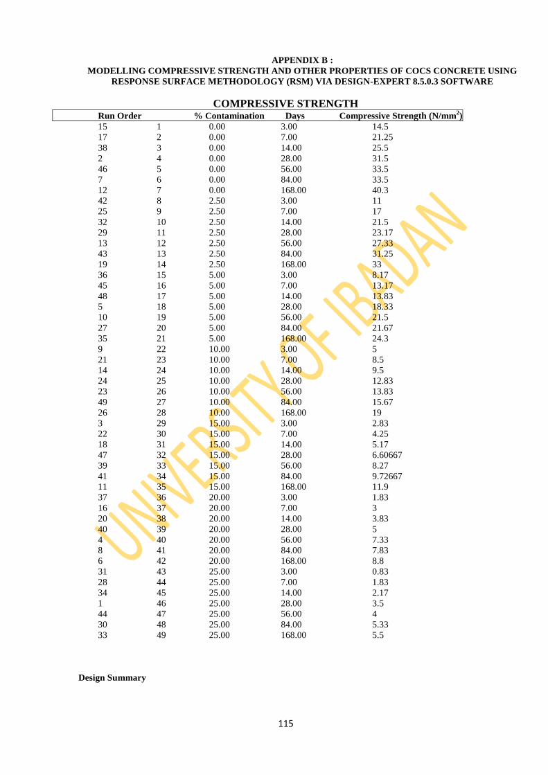
115
APPENDIX B :
MODELLING COMPRESSIVE STRENGTH AND OTHER PROPERTIES OF COCS CONCRETE USING
RESPONSE SURFACE METHODOLOGY (RSM) VIA DESIGN-EXPERT 8.5.0.3 SOFTWARE
COMPRESSIVE STRENGTH Run Order % Contamination Days Compressive Strength (N/mm
2)
15 1 0.00 3.00 14.5
17 2 0.00 7.00 21.25
38 3 0.00 14.00 25.5
2 4 0.00 28.00 31.5
46 5 0.00 56.00 33.5
7 6 0.00 84.00 33.5
12 7 0.00 168.00 40.3
42 8 2.50 3.00 11
25 9 2.50 7.00 17
32 10 2.50 14.00 21.5
29 11 2.50 28.00 23.17
13 12 2.50 56.00 27.33
43 13 2.50 84.00 31.25
19 14 2.50 168.00 33
36 15 5.00 3.00 8.17
45 16 5.00 7.00 13.17
48 17 5.00 14.00 13.83
5 18 5.00 28.00 18.33
10 19 5.00 56.00 21.5
27 20 5.00 84.00 21.67
35 21 5.00 168.00 24.3
9 22 10.00 3.00 5
21 23 10.00 7.00 8.5
14 24 10.00 14.00 9.5
24 25 10.00 28.00 12.83
23 26 10.00 56.00 13.83
49 27 10.00 84.00 15.67
26 28 10.00 168.00 19
3 29 15.00 3.00 2.83
22 30 15.00 7.00 4.25
18 31 15.00 14.00 5.17
47 32 15.00 28.00 6.60667
39 33 15.00 56.00 8.27
41 34 15.00 84.00 9.72667
11 35 15.00 168.00 11.9
37 36 20.00 3.00 1.83
16 37 20.00 7.00 3
20 38 20.00 14.00 3.83
40 39 20.00 28.00 5
4 40 20.00 56.00 7.33
8 41 20.00 84.00 7.83
6 42 20.00 168.00 8.8
31 43 25.00 3.00 0.83
28 44 25.00 7.00 1.83
34 45 25.00 14.00 2.17
1 46 25.00 28.00 3.5
44 47 25.00 56.00 4
30 48 25.00 84.00 5.33
33 49 25.00 168.00 5.5
Design Summary

116
Study Type Response Surface Runs 49
Design Type Central Composite Blocks No Blocks
Design Model Quadratic Build Time (ms) 4.45
Factor Name Units Type Subtype Min. Max. Coded Values Mean
Std. Dev. A Conta. % Numeric Contin. 0.00 25.00 -1.000=0.00 1.000=25.00 11.07 8.65
B Days No Numeric Contin. 3.00 168.00 -1.000=3.00 1.000=168.00 51.43 54.69
Resp. Name Units Obs Analysis Min Max Mean Std. Dev. Ratio Trans Model Y1 Compr. Str.N/mm
2 49 Polynomia l0.83 40.3 13.8599 10.371 48.5542 None Sixth
Response 1 Compressive Strength
ANOVA for Response Surface Sixth Model
Analysis of variance table [Partial sum of squares - Type III] Sum of Mean F p-value significant
Source Squares df Squar Value Prob > F Model 5146.02 27 190.59 239.74 < 0.0001
A-Cont. 48.05 1 48.05 60.44 < 0.0001
B-Days 4.55 1 4.55 5.72 0.0262
AB 0.60 1 0.60 0.75 0.3964
A2 1.45 1 1.45 1.83 0.1910
B2 4.53 1 4.53 5.70 0.0264
A2B 0.060 1 0.060 0.075 0.7869
AB2 1.82 1 1.82 2.29 0.1453
A3 4.07 1 4.07 5.12 0.0344
B3 4.77 1 4.77 5.99 0.0232
A2B2 0.19 1 0.19 0.24 0.6298
A3B 0.16 1 0.16 0.20 0.6610
AB3 3.34 1 3.34 4.20 0.0530
A4 10.42 1 10.42 13.11 0.0016
B4 2.72 1 2.72 3.43 0.0783
A3B2 0.51 1 0.51 0.64 0.4333
A2B3 0.019 1 0.019 0.024 0.8789
A4B 0.19 1 0.19 0.24 0.6328
AB4 1.61 1 1.61 2.03 0.1691
A5 5.71 1 5.71 7.18 0.0140
B5 4.71 1 4.71 5.93 0.0239
A3B3 1.44 1 1.44 1.81 0.1926
A4B2 2.59 1 2.59 3.26 0.0853
A2B4 1.20 1 1.20 1.51 0.2333
A5B 0.076 1 0.076 0.095 0.7608
AB5 2.66 1 2.66 3.34 0.0818
A6 12.18 1 12.18 15.33 0.0008
B6 4.97 1 4.97 6.26 0.0207
Residual 16.70 21 0.80
Cor Total 5162.72 48
The Model F-value of 239.74 implies the model is significant. There is only
a 0.01% chance that a "Model F-Value" this large could occur due to noise.
Values of "Prob > F" less than 0.0500 indicate model terms are significant.
In this case A, B, B2, A3, B3, A4, A5, B5, A6, B6 are significant
model terms.
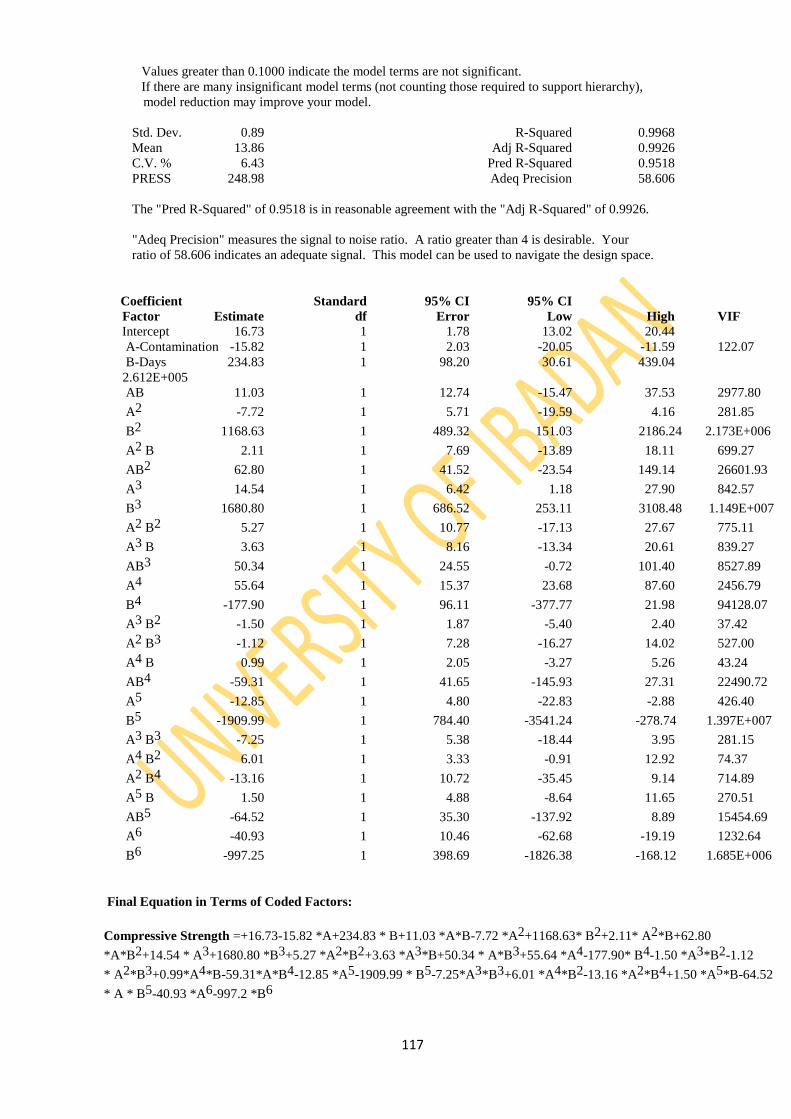
117
Values greater than 0.1000 indicate the model terms are not significant.
If there are many insignificant model terms (not counting those required to support hierarchy),
model reduction may improve your model.
Std. Dev. 0.89 R-Squared 0.9968
Mean 13.86 Adj R-Squared 0.9926
C.V. % 6.43 Pred R-Squared 0.9518
PRESS 248.98 Adeq Precision 58.606
The "Pred R-Squared" of 0.9518 is in reasonable agreement with the "Adj R-Squared" of 0.9926.
"Adeq Precision" measures the signal to noise ratio. A ratio greater than 4 is desirable. Your
ratio of 58.606 indicates an adequate signal. This model can be used to navigate the design space.
Coefficient Standard 95% CI 95% CI
Factor Estimate df Error Low High VIF Intercept 16.73 1 1.78 13.02 20.44
A-Contamination -15.82 1 2.03 -20.05 -11.59 122.07
B-Days 234.83 1 98.20 30.61 439.04
2.612E+005
AB 11.03 1 12.74 -15.47 37.53 2977.80
A2 -7.72 1 5.71 -19.59 4.16 281.85
B2 1168.63 1 489.32 151.03 2186.24 2.173E+006
A2 B 2.11 1 7.69 -13.89 18.11 699.27
AB2 62.80 1 41.52 -23.54 149.14 26601.93
A3 14.54 1 6.42 1.18 27.90 842.57
B3 1680.80 1 686.52 253.11 3108.48 1.149E+007
A2 B2 5.27 1 10.77 -17.13 27.67 775.11
A3 B 3.63 1 8.16 -13.34 20.61 839.27
AB3 50.34 1 24.55 -0.72 101.40 8527.89
A4 55.64 1 15.37 23.68 87.60 2456.79
B4 -177.90 1 96.11 -377.77 21.98 94128.07
A3 B2 -1.50 1 1.87 -5.40 2.40 37.42
A2 B3 -1.12 1 7.28 -16.27 14.02 527.00
A4 B 0.99 1 2.05 -3.27 5.26 43.24
AB4 -59.31 1 41.65 -145.93 27.31 22490.72
A5 -12.85 1 4.80 -22.83 -2.88 426.40
B5 -1909.99 1 784.40 -3541.24 -278.74 1.397E+007
A3 B3 -7.25 1 5.38 -18.44 3.95 281.15
A4 B2 6.01 1 3.33 -0.91 12.92 74.37
A2 B4 -13.16 1 10.72 -35.45 9.14 714.89
A5 B 1.50 1 4.88 -8.64 11.65 270.51
AB5 -64.52 1 35.30 -137.92 8.89 15454.69
A6 -40.93 1 10.46 -62.68 -19.19 1232.64
B6 -997.25 1 398.69 -1826.38 -168.12 1.685E+006
Final Equation in Terms of Coded Factors:
Compressive Strength =+16.73-15.82 *A+234.83 * B+11.03 *A*B-7.72 *A2+1168.63* B2+2.11* A2*B+62.80
*A*B2+14.54 * A3+1680.80 *B3+5.27 *A2*B2+3.63 *A3*B+50.34 * A*B3+55.64 *A4-177.90* B4-1.50 *A3*B2-1.12
* A2*B3+0.99*A4*B-59.31*A*B4-12.85 *A5-1909.99 * B5-7.25*A3*B3+6.01 *A4*B2-13.16 *A2*B4+1.50 *A5*B-64.52
* A * B5-40.93 *A6-997.2 *B6

118
Response 1 Compressive Strength Transform: None
Diagnostics Case Statistics
Internally Externally Influence on
Standard Actual Predicted Studentized Studentized Fitted Value Cook's Run
Order Value Value Residual Leverage Residual Residual DFFITS Distance Order 1 3.50 3.50 7.964E-004 0.762 0.002 0.002 0.003 0.000 46
2 31.50 30.70 0.80 0.647 1.514 1.565 * 2.12 0.150 4
3 2.83 2.30 0.53 0.500 0.834 0.828 0.828 0.025 29
4 7.33 7.07 0.26 0.559 0.441 0.432 0.487 0.009 40
5 18.33 17.92 0.41 0.412 0.603 0.594 0.497 0.009 18
6 8.80 8.65 0.15 0.965 0.896 0.892 * 4.71 0.799 42
7 33.50 34.18 -0.68 0.873 -2.129 -2.346 * -6.14 * 1.11 6
8 7.83 7.87 -0.036 0.726 -0.078 -0.076 -0.124 0.001 41
9 5.00 5.72 -0.72 0.480 -1.121 -1.128 -1.084 0.041 22
10 21.50 20.93 0.57 0.433 0.855 0.849 0.743 0.020 19
11 11.90 12.33 -0.43 0.862 -1.298 -1.321 * -3.30 0.376 35
12 40.30 40.32 -0.022 0.975 -0.161 -0.157 -0.991 0.037 7
13 27.33 27.88 -0.55 0.444 -0.831 -0.824 -0.736 0.020 12
14 9.50 9.84 -0.34 0.365 -0.485 -0.476 -0.361 0.005 24
15 14.50 14.59 -0.094 0.690 -0.189 -0.185 -0.276 0.003 1
16 3.00 3.40 -0.40 0.425 -0.589 -0.580 -0.499 0.009 37
17 21.25 21.03 0.22 0.445 0.333 0.326 0.292 0.003 2
18 5.17 4.92 0.25 0.383 0.361 0.353 0.279 0.003 31
19 33.00 32.68 0.32 0.707 0.656 0.647 1.006 0.037 14
20 3.83 3.53 0.30 0.417 0.437 0.429 0.363 0.005 38
21 8.50 8.77 -0.27 0.369 -0.381 -0.373 -0.285 0.003 23
22 4.25 4.57 -0.32 0.381 -0.453 -0.444 -0.348 0.005 30
23 13.83 14.10 -0.27 0.497 -0.428 -0.419 -0.417 0.006 26
24 12.83 11.82 1.01 0.401 1.466 1.510 1.236 0.051 25
25 17.00 17.01 -0.014 0.364 -0.019 -0.019 -0.014 0.000 9
26 19.00 18.38 0.62 0.792 1.530 1.584 * 3.09 0.318 28
27 21.67 22.82 -1.15 0.539 -1.897 -2.033 * -2.20 0.150 20
28 1.83 2.16 -0.33 0.468 -0.500 -0.491 -0.461 0.008 44
29 23.17 24.78 -1.61 0.413 -2.350 -2.671 * -2.24 0.139 11
30 5.33 5.36 -0.028 0.962 -0.160 -0.156 -0.781 0.023 48
31 0.83 0.82 8.837E-003 0.778 0.021 0.021 0.038 0.000 43
32 21.50 20.76 0.74 0.380 1.055 1.057 0.828 0.024 10
33 5.50 5.52 -0.018 0.998 -0.508 -0.499 * -12.24 * 5.55 49
34 2.17 1.79 0.38 0.582 0.667 0.658 0.776 0.022 45
35 24.30 24.92 -0.62 0.625 -1.131 -1.139 -1.470 0.076 21
36 8.17 7.59 0.58 0.441 0.872 0.867 0.770 0.021 15
37 1.83 1.53 0.30 0.578 0.516 0.507 0.593 0.013 36
38 25.50 25.92 -0.42 0.502 -0.675 -0.666 -0.669 0.016 3
39 8.27 8.45 -0.18 0.499 -0.293 -0.286 -0.285 0.003 33
40 5.00 5.57 -0.57 0.504 -0.911 -0.907 -0.915 0.030 39
41 9.73 9.52 0.20 0.583 0.354 0.347 0.410 0.006 34
42 11.00 11.60 -0.60 0.454 -0.911 -0.907 -0.828 0.025 8
43 31.25 29.54 1.71 0.495 2.707 3.274 * 3.24 0.257 13
44 4.00 4.02 -0.022 0.878 -0.072 -0.070 -0.189 0.001 47
45 13.17 12.07 1.10 0.349 1.535 1.590 1.165 0.045 16
46 33.50 33.30 0.20 0.746 0.434 0.426 0.730 0.020 5
47 6.61 6.66 -0.050 0.425 -0.074 -0.073 -0.062 0.000 32
48 13.83 14.74 -0.91 0.345 -1.255 -1.274 -0.925 0.030 17
49 15.67 15.70 -0.029 0.580 -0.051 -0.049 -0.058 0.000 27
* Exceeds limits
Current Transform: None
Box-Cox Power Transformation

119
Constant 95% CI 95% CI Best Rec.
k Low High LambdaTransform 0.000 -1.000E-002 0.44 0.21 Log
Transformation:
Response 1: Compressive Strength Transform: Base 10 Log Constant: 0
Fit Summary (detailed tables shown below)
Sequential Lack of Fit Adjusted Predicted
Source p-value p-value R-Squared R-Squared Linear < 0.0001 0.8902 0.8788
2FI 0.0549 0.8966 0.8800
Quadratic < 0.0001 0.9514 0.9421
Cubic < 0.0001 0.9745 0.9664
Quartic 0.0014 0.9833 0.9758
Fifth 0.0149 0.9880 0.9723
Sixth < 0.0001 0.9959 0.9764 Suggested
Sequential Model Sum of Squares [Type I]
Sum of Mean Fp-value
Source Squares df Square ValueProb > F Mean vs Total 48.48 1 48.48
Linear vs Mean 6.74 2 3.37 195.51< 0.0001
2FI vs Linear 0.063 1 0.063 3.880.0549
Quadratic vs 2FI 0.40 2 0.20 26.35< 0.0001
Cubic vs Quadratic 0.17 4 0.043 10.74< 0.0001
Quartic vs Cubic 0.067 5 0.013 5.090.0014
Fifth vs Quartic 0.037 6 6.110E-003 3.250.0149
Sixth vs Fifth 0.039 7 5.567E-003 8.56 < 0.0001 Suggested
Residual 0.014 21 6.505E-004
Total 56.01 49 1.14
"Sequential Model Sum of Squares [Type I]": Select the highest order polynomial where the
additional terms are significant and the model is not aliased.
Model Summary Statistics
Std. Adjusted Predicted
Source Dev. R-Squared R-Squared R-Squared PRESS Linear 0.13 0.8947 0.8902 0.8788 0.91
2FI 0.13 0.9031 0.8966 0.8800 0.90
Quadratic 0.087 0.9565 0.9514 0.9421 0.44
Cubic 0.063 0.9793 0.9745 0.9664 0.25
Quartic 0.051 0.9881 0.9833 0.9758 0.18
Fifth 0.043 0.9930 0.9880 0.9723 0.21
Sixth 0.026 0.9982 0.9959 0.9764 0.18 Suggested
"Model Summary Statistics": Focus on the model maximizing the "Adjusted R-Squared"
and the "Predicted R-Squared".
Response 1 Compressive Strength
Transform: Base 10 Log Constant: 0
ANOVA for Response Surface Sixth Model
Analysis of variance table [Partial sum of squares - Type III]

120
Sum of Mean F p-value
Source Squares df Square Value Prob > F Model 7.52 27 0.28 428.18 < 0.0001significant
A-Contamination 0.058 1 0.058 89.60 < 0.0001
B-Days 0.022 1 0.022 33.65 < 0.0001
AB 7.435E-005 1 7.435E-005 0.11 0.7386
A2 2.312E-003 1 2.312E-003 3.55 0.0733
B2 0.022 1 0.022 34.31 < 0.0001
A2B 4.733E-004 1 4.733E-004 0.73 0.4033
AB2 5.622E-005 1 5.622E-005 0.086 0.7716
A3 0.010 1 0.010 15.86 0.0007
B3 0.024 1 0.024 36.37 < 0.0001
A2B2 7.734E-004 1 7.734E-004 1.19 0.2879
A3B 4.348E-004 1 4.348E-004 0.67 0.4228
AB3 3.007E-004 1 3.007E-004 0.46 0.5040
A4 7.907E-003 1 7.907E-003 12.16 0.0022
B4 0.012 1 0.012 18.48 0.0003
A3B2 7.486E-005 1 7.486E-005 0.12 0.7378
A2B3 7.276E-004 1 7.276E-004 1.12 0.3023
A4B 3.817E-004 1 3.817E-004 0.59 0.4522
AB4 3.076E-005 1 3.076E-005 0.047 0.8299
A5 0.012 1 0.012 18.44 0.0003
B5 0.023 1 0.023 35.89 < 0.0001
A3B3 5.157E-005 1 5.157E-005 0.079 0.7810
A4B2 1.192E-003 1 1.192E-003 1.83 0.1902
A2B4 1.983E-003 1 1.983E-003 3.05 0.0954
A5B 3.617E-004 1 3.617E-004 0.56 0.4641
AB5 1.482E-004 1 1.482E-004 0.23 0.6380
A6 0.010 1 0.010 15.80 0.0007
B6 0.025 1 0.025 38.36 < 0.0001
Residual 0.014 21 6.505E-004
Cor Total 7.53 48
The Model F-value of 428.18 implies the model is significant. There is only
a 0.01% chance that a "Model F-Value" this large could occur due to noise.
Values of "Prob > F" less than 0.0500 indicate model terms are significant.
In this case A, B, B2, A3, B3, A4, B4, A5, B5,
A6, B6 are significant model terms.
Values greater than 0.1000 indicate the model terms are not significant.
If there are many insignificant model terms (not counting those required to support hierarchy),
model reduction may improve your model.
Std. Dev. 0.026 R-Squared 0.9982
Mean 0.99 Adj R-Squared 0.9959
C.V. % 2.56 Pred R-Squared 0.9764
PRESS 0.18 Adeq Precision 86.018
The "Pred R-Squared" of 0.9764 is in reasonable agreement with the "Adj R-Squared" of 0.9959.
"Adeq Precision" measures the signal to noise ratio. A ratio greater than 4 is desirable. Your
ratio of 86.018 indicates an adequate signal. This model can be used to navigate the design space.
Coefficient Standard 95% CI 95% CI

121
Factor Estimate df Error Low High VIF Intercept 1.37 1 0.051 1.26 1.47
A-Contamination -0.55 1 0.058 -0.67 -0.43 122.07
B-Days 16.29 1 2.81 10.45 22.14 2.612E+005
AB 0.12 1 0.36 -0.63 0.88 2977.80
A2 -0.31 1 0.16 -0.65 0.032 281.85
B2 81.98 1 14.00 52.87 111.09 2.173E+006
A2 B 0.19 1 0.22 -0.27 0.65 699.27
AB2 -0.35 1 1.19 -2.82 2.12 26601.93
A3 0.73 1 0.18 0.35 1.11 842.57
B3 118.42 1 19.64 77.58 159.26 1.149E+007
A2 B2 0.34 1 0.31 -0.30 0.98 775.11
A3 B -0.19 1 0.23 -0.68 0.29 839.27
AB3 -0.48 1 0.70 -1.94 0.98 8527.89
A4 1.53 1 0.44 0.62 2.45 2456.79
B4 -11.82 1 2.75 -17.53 -6.10 94128.07
A3 B2 -0.018 1 0.054 -0.13 0.093 37.42
A2 B3 -0.22 1 0.21 -0.65 0.21 527.00
A4 B 0.045 1 0.059 -0.077 0.17 43.24
AB4 0.26 1 1.19 -2.22 2.74 22490.72
A5 -0.59 1 0.14 -0.87 -0.30 426.40
B5 -134.42 1 22.44 -181.08 -87.76 1.397E+007
A3 B3 0.043 1 0.15 -0.28 0.36 281.15
A4 B2 0.13 1 0.095 -0.069 0.33 74.37
A2 B4 -0.54 1 0.31 -1.17 0.10 714.89
A5 B 0.10 1 0.14 -0.19 0.39 270.51
AB5 0.48 1 1.01 -1.62 2.58 15454.69
A6 -1.19 1 0.30 -1.81 -0.57 1232.64
B6 -70.64 1 11.40 -94.35 -46.92 1.685E+006
Final Equation in Terms of Coded Factors:
Log10(Compressive Strength) = +1.37-0.55 * A+16.29 * B+0.12 * A * B-0.31 * A2+81.98 * B2+0.19* A2 *B-0.35 * A
* B2+0.73 * A3+118.42 * B3+0.34 * A2* B2-0.19 * A*B-0.48 * A * B3+1.53 *A-11.82 *B4-0.018 *A3*B2-0.22 *A2
*B3+0.045 * A4 *B+0.26 *A*B4-0.59 *A5-134.42 *B5+0.043 *A3*B3+0.13 *A4*B2-0.54 *A2*B4+0.10 *A5 *B+0.48
*A*B5-1.19 *A6-70.64* B6

122
Design-Expert® SoftwareLog10(Compressive Strength)
Color points by value ofLog10(Compressive Strength):
1.60531
-0.0809219
Internally Studentized Residuals
No
rma
l %
Pro
ba
bilit
y
Normal Plot of Residuals
-3.00 -2.00 -1.00 0.00 1.00 2.00 3.00
1
5
10
20
30
50
70
80
90
95
99
Design-Expert® SoftwareLog10(Compressive Strength)
Color points by value ofLog10(Compressive Strength):
1.60531
-0.0809219
Predicted
Inte
rna
lly
Stu
de
nti
ze
d R
es
idu
als
Residuals vs. Predicted
-3.00
-2.00
-1.00
0.00
1.00
2.00
3.00
-0.50 0.00 0.50 1.00 1.50 2.00

123
Design-Expert® SoftwareLog10(Compressive Strength)
Color points by value ofLog10(Compressive Strength):
1.60531
-0.0809219
Run Number
Inte
rna
lly
Stu
de
nti
ze
d R
es
idu
als
Residuals vs. Run
-3.00
-2.00
-1.00
0.00
1.00
2.00
3.00
1 7 13 19 25 31 37 43 49
Design-Expert® SoftwareLog10(Compressive Strength)
Color points by value ofLog10(Compressive Strength):
1.60531
-0.0809219
Actual
Pre
dic
ted
Predicted vs. Actual
-0.50
0.00
0.50
1.00
1.50
2.00
-0.50 0.00 0.50 1.00 1.50 2.00

124
Design-Expert® SoftwareLog10(Compressive Strength)
LambdaCurrent = 0Best = 0.21Low C.I. = -0.01High C.I. = 0.44
Recommend transform:Log (Lambda = 0)
Lambda
Ln
(Re
sid
ua
lSS
)
Box-Cox Plot for Power Transforms
0.00
5.00
10.00
15.00
20.00
-3 -2 -1 0 1 2 3
Design-Expert® SoftwareLog10(Compressive Strength)
Color points by value ofLog10(Compressive Strength):
1.60531
-0.0809219
Contamination
Inte
rna
lly
Stu
de
nti
ze
d R
es
idu
als
Residuals vs. Contamination
-3.00
-2.00
-1.00
0.00
1.00
2.00
3.00
0.00 5.00 10.00 15.00 20.00 25.00

125
Design-Expert® SoftwareLog10(Compressive Strength)
Color points by value ofLog10(Compressive Strength):
1.60531
-0.0809219
Run Number
Ex
tern
ally
Stu
de
nti
ze
d R
es
idu
als
Externally Studentized Residuals
-4.00
-2.00
0.00
2.00
4.00
1 7 13 19 25 31 37 43 49
Design-Expert® SoftwareLog10(Compressive Strength)
Color points by value ofLog10(Compressive Strength):
1.60531
-0.0809219
Run Number
Le
ve
rag
e
Leverage vs. Run
0.00
0.20
0.40
0.60
0.80
1.00
1 7 13 19 25 31 37 43 49

126
Design-Expert® SoftwareLog10(Compressive Strength)
Color points by value ofLog10(Compressive Strength):
1.60531
-0.0809219
Run Number
DF
FIT
S
DFFITS vs. Run
-10.00
-5.00
0.00
5.00
10.00
1 7 13 19 25 31 37 43 49
Design-Expert® SoftwareLog10(Compressive Strength)
Color points by value ofLog10(Compressive Strength):
1.60531
-0.0809219
Run Number
DF
BE
TA
S f
or
Inte
rce
pt
DFBETAS for Intercept vs. Run
-2.00
-1.00
0.00
1.00
2.00
1 7 13 19 25 31 37 43 49

127
Design-Expert® SoftwareLog10(Compressive Strength)
Color points by value ofLog10(Compressive Strength):
1.60531
-0.0809219
Run Number
Co
ok
's D
ista
nc
e
Cook's Distance
0.00
0.50
1.00
1.50
2.00
2.50
1 7 13 19 25 31 37 43 49
Response 1 Compressive Strength Transform: Base 10 Log Constant: 0.000
Diagnostics Case Statistics
Internally Externally Influence on
Standard Actual Predicted Studentized Studentized Fitted Value Cook's Run
Order Value Value Residual Leverage Residual Residual DFFITS Distance Order 1 0.54 0.53 0.018 0.762 1.459 1.502 * 2.69 0.244 46
2 1.50 1.49 6.224E-003 0.647 0.411 0.403 0.545 0.011 4
3 0.45 0.43 0.021 0.500 1.160 1.170 1.171 0.048 29
4 0.87 0.83 0.035 0.559 2.044 2.228 * 2.51 0.189 40
5 1.26 1.26 5.086E-003 0.412 0.260 0.254 0.213 0.002 18
6 0.94 0.94 1.224E-003 0.965 0.258 0.252 1.330 0.066 42
7 1.53 1.54 -0.012 0.873 -1.367 -1.397 * -3.66 0.458 6
8 0.89 0.91 -0.015 0.726 -1.121 -1.128 -1.835 0.119 41
9 0.70 0.72 -0.026 0.480 -1.414 -1.451 -1.394 0.066 22
10 1.33 1.32 8.723E-003 0.433 0.454 0.446 0.390 0.006 19
11 1.08 1.08 -2.594E-003 0.862 -0.274 -0.268 -0.670 0.017 35
12 1.61 1.61 2.890E-004 0.975 0.072 0.071 0.445 0.007 7
13 1.44 1.45 -0.012 0.444 -0.618 -0.608 -0.543 0.011 12
14 0.98 0.98 8.455E-004 0.365 0.042 0.041 0.031 0.000 24
15 1.16 1.15 0.014 0.690 0.958 0.956 1.426 0.073 1
16 0.48 0.49 -9.575E-003 0.425 -0.495 -0.486 -0.418 0.006 37
17 1.33 1.35 -0.023 0.445 -1.187 -1.199 -1.073 0.040 2
18 0.71 0.71 2.785E-003 0.383 0.139 0.136 0.107 0.000 31
19 1.52 1.52 1.802E-003 0.707 0.131 0.127 0.198 0.001 14
20 0.58 0.58 -9.679E-004 0.417 -0.050 -0.049 -0.041 0.000 38
21 0.93 0.92 4.610E-003 0.369 0.227 0.222 0.170 0.001 23
22 0.63 0.64 -0.015 0.381 -0.756 -0.748 -0.587 0.013 30
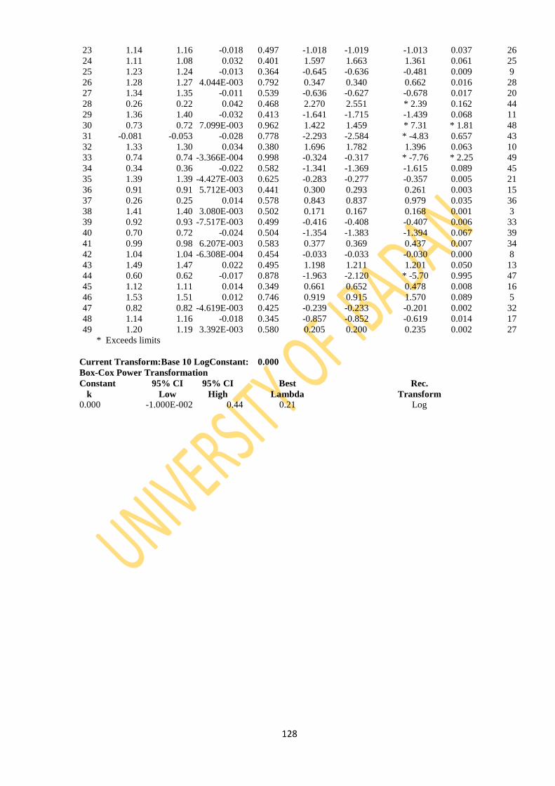
128
23 1.14 1.16 -0.018 0.497 -1.018 -1.019 -1.013 0.037 26
24 1.11 1.08 0.032 0.401 1.597 1.663 1.361 0.061 25
25 1.23 1.24 -0.013 0.364 -0.645 -0.636 -0.481 0.009 9
26 1.28 1.27 4.044E-003 0.792 0.347 0.340 0.662 0.016 28
27 1.34 1.35 -0.011 0.539 -0.636 -0.627 -0.678 0.017 20
28 0.26 0.22 0.042 0.468 2.270 2.551 * 2.39 0.162 44
29 1.36 1.40 -0.032 0.413 -1.641 -1.715 -1.439 0.068 11
30 0.73 0.72 7.099E-003 0.962 1.422 1.459 * 7.31 * 1.81 48
31 -0.081 -0.053 -0.028 0.778 -2.293 -2.584 * -4.83 0.657 43
32 1.33 1.30 0.034 0.380 1.696 1.782 1.396 0.063 10
33 0.74 0.74 -3.366E-004 0.998 -0.324 -0.317 * -7.76 * 2.25 49
34 0.34 0.36 -0.022 0.582 -1.341 -1.369 -1.615 0.089 45
35 1.39 1.39 -4.427E-003 0.625 -0.283 -0.277 -0.357 0.005 21
36 0.91 0.91 5.712E-003 0.441 0.300 0.293 0.261 0.003 15
37 0.26 0.25 0.014 0.578 0.843 0.837 0.979 0.035 36
38 1.41 1.40 3.080E-003 0.502 0.171 0.167 0.168 0.001 3
39 0.92 0.93 -7.517E-003 0.499 -0.416 -0.408 -0.407 0.006 33
40 0.70 0.72 -0.024 0.504 -1.354 -1.383 -1.394 0.067 39
41 0.99 0.98 6.207E-003 0.583 0.377 0.369 0.437 0.007 34
42 1.04 1.04 -6.308E-004 0.454 -0.033 -0.033 -0.030 0.000 8
43 1.49 1.47 0.022 0.495 1.198 1.211 1.201 0.050 13
44 0.60 0.62 -0.017 0.878 -1.963 -2.120 * -5.70 0.995 47
45 1.12 1.11 0.014 0.349 0.661 0.652 0.478 0.008 16
46 1.53 1.51 0.012 0.746 0.919 0.915 1.570 0.089 5
47 0.82 0.82 -4.619E-003 0.425 -0.239 -0.233 -0.201 0.002 32
48 1.14 1.16 -0.018 0.345 -0.857 -0.852 -0.619 0.014 17
49 1.20 1.19 3.392E-003 0.580 0.205 0.200 0.235 0.002 27
* Exceeds limits
Current Transform:Base 10 LogConstant: 0.000
Box-Cox Power Transformation
Constant 95% CI 95% CI Best Rec.
k Low High Lambda Transform 0.000 -1.000E-002 0.44 0.21 Log

129
Design-Expert® SoftwareFactor Coding: ActualOriginal ScaleCompressive Strength
Design Points40.3
0.83
X1 = A: ContaminationX2 = B: Days
0.00 5.00 10.00 15.00 20.00 25.00
3.00
36.00
69.00
102.00
135.00
168.00
Compressive Strength
A: Contamination
B:
Da
ys
5E+0611E+062
Design-Expert® SoftwareFactor Coding: ActualOriginal ScaleCompressive Strength
Actual FactorsA: Contamination = 12.50B: Days = 85.50
Perturbation
Deviation from Reference Point (Coded Units)
Co
mp
res
siv
e S
tre
ng
th
-1.000 -0.500 0.000 0.500 1.000
2.34152
4.71023E+060
9.42046E+060
1.41307E+061
1.88409E+061
2.35512E+061
2.82614E+061
A AB B

130
Design-Expert® SoftwareCompressive Strength
Color points by value ofCompressive Strength:
40.3
0.83
Actual
Pre
dic
ted
Predicted vs. Actual
0.00
10.00
20.00
30.00
40.00
50.00
0.00 10.00 20.00 30.00 40.00 50.00
Design-Expert® SoftwareFactor Coding: ActualOriginal ScaleCompressive Strength
Design points above predicted valueDesign points below predicted value40.3
0.83
X1 = A: ContaminationX2 = B: Days
3.00
36.00
69.00
102.00
135.00
168.00
0.00
5.00
10.00
15.00
20.00
25.00
0.794103
4.30555E+061
8.6111E+061
1.29167E+062
1.72222E+062
C
om
pre
ss
ive
Str
en
gth
A: Contamination B: Days

131
Model B (others)
Design Summary
File Version 8.0.5.2
Study Type Response Surface Runs 7 Analysis Polynomial
Design Type One Factor Blocks No Blocks Trans None
Design Model Quadratic Build Time (ms) 6.16
Factor Name Units Type Sub-
type
Actual Values Coded Values Mean
Std.
Dev. Min Max Min Max
A Crude
Oil % Numeric Cont. 0.00 25.00 -1.00 1.00 10.11 9.52
Response Name Units Min. Max. Mean Std. Dev. Ratio Model
Y1 Slump mm 30 200 106.429 61.3538 6.6667 Quadratic
Y2 C.F. Ratio 0.45 0.85 0.6686 0.1536 1.8889 Linear
Y3 Flow mm 230 370 284.286 58.4828 1.6087 Inverse Fifth
Y4 Flex St. N/mm2 0.113 5.865 3.298 2.2701 51.9027
Inverse Sqrt
Quartic
Y5 Perm. Kg 0 0.15 0.0557 0.05740 N/A Sqrt Quadratic
Y6 L. S. mm 0.02 0.09 0.0543 0.0263 4.5 Sqrt Fifth
Y7 Resist. 25.07 32.31 28.7857 2.5347 1.2888 Linear
SLUMP
Response 1 Slump Transform: None
Summary (detailed tables shown below)
Sequential Lack of Fit Adjusted Predicted
Source p-value p-value R-Squared R-Squared
Linear 0.0003 0.9282 0.8836 Suggested
Quadratic 0.3439 0.9302 0.8831
Cubic 0.9737 0.9070 0.3285
Quartic 0.2392 0.9413 -7.9099
Fifth 0.0759 0.9983
Sixth
Sequential Model Sum of Squares [Type I]
Sum of Mean F p-value
Source Squares df Square Value Prob > F Mean vs Total 79289.29 1 79289.29
Linear vs Mean 21233.51 1 21233.51 78.51 0.0003 Suggested
Quadratic vs Linear 301.95 1 301.95 1.15 0.3439
Cubic vs Quadratic 0.45 1 0.45 1.281E-003 0.9737
Quartic vs Cubic 607.69 1 607.69 2.75 0.2392
Fifth vs Quartic 435.87 1 435.87 69.77 0.0759
Sixth vs Fifth 6.25 1 6.25
Residual 0.000 0
Total 1.019E+005 7 14553.57

132
"Sequential Model Sum of Squares [Type I]": Select the highest order polynomial where the
additional terms are significant and the model is not aliased.
Model Summary Statistics
Std. Adjusted Predicted
Source Dev. R-Squared R-Squared R-Squared PRESS Linear 16.45 0.9401 0.9282 0.8836 2627.93 Suggested
Quadratic 16.20 0.9535 0.9302 0.8831 2639.90
Cubic 18.71 0.9535 0.9070 0.3285 15165.59
Quartic 14.87 0.9804 0.9413 -7.9099 2.012E+005
Fifth 2.50 0.9997 0.9983 +
Sixth +
+ Case(s) with leverage of 1.0000: PRESS statistic not defined
Response 1 Slump
ANOVA for Response Surface Quadratic Model
Analysis of variance table [Partial sum of squares - Type III]
Sum of Mean F p-value
Source Squares df Square Value Prob > F Model 21535.46 2 10767.73 41.01 0.0022 significant
A-Crude Oil 20362.70 1 20362.70 77.55 0.0009
A2 301.95 1 301.95 1.15 0.3439
Residual 1050.26 4 262.56
Cor Total 22585.71 6
The Model F-value of 41.01 implies the model is significant. There is only
a 0.22% chance that a "Model F-Value" this large could occur due to noise.
Std. Dev. 16.20 R-Squared 0.9535
Mean 106.43 Adj R-Squared 0.9302
C.V. % 15.23 Pred R-Squared 0.8831
PRESS 2639.90 Adeq Precision 14.237
The "Pred R-Squared" of 0.8831 is in reasonable agreement with the "Adj R-Squared" of 0.9302.
"Adeq Precision" measures the signal to noise ratio. A ratio greater than 4 is desirable. Your
ratio of 14.237 indicates an adequate signal. This model can be used to navigate the design space.
Coefficient Standard 95% CI 95% CI
Factor Estimate df Error Low High VIF Intercept 110.55 1 11.02 79.96 141.14
A-Crude Oil 75.51 1 8.57 51.71 99.32 1.14
A2 16.70 1 15.57 -26.53 59.92 1.14
Final Equation in Terms of Coded Factors:
Slump = +110.55+75.51 * A+16.70 * A2
Response 1 Slump Transform: None
Diagnostics Case Statistics
Internally Externally Influence on
Standard Actual Predicted Studentized Studentized Fitted Value Cook's Run
Order Value Value Residual Leverage Residual Residual DFFITS Distance Order 1 170.00 161.87 8.13 0.307 0.603 0.548 0.365 0.054 6

133
2 120.00 126.32 -6.32 0.413 -0.509 -0.456 -0.382 0.061 5
3 30.00 51.73 -21.73 0.353 -1.667 -2.612 -1.928 0.504 1
4 75.00 53.62 21.38 0.308 1.587 2.256 1.506 0.374 3
5 55.00 52.58 2.42 0.331 0.182 0.159 0.112 0.005 2
6 95.00 96.12 -1.12 0.451 -0.093 -0.081 -0.073 0.002 4
7 200.00 202.76 -2.76 0.837 -0.422 -0.374 -0.847 0.305 7
Current Transform: None
Box-Cox Power Transformation
Constant 95% CI 95% CI Best Rec.
k Low High Lambda Transform 0.000 0.63 3.72 2.23 None
Response 1 Slump Transform: None
Diagnostics Case Statistics
Internally Externally Influence on
Standard Actual Predicted Studentized Studentized Fitted Value Cook's Run
Order Value Value Residual Leverage Residual Residual DFFITS Distance Order 1 170.00 161.87 8.13 0.307 0.603 0.548 0.365 0.054 6
2 120.00 126.32 -6.32 0.413 -0.509 -0.456 -0.382 0.061 5
3 30.00 51.73 -21.73 0.353 -1.667 -2.612 -1.928 0.504 1
4 75.00 53.62 21.38 0.308 1.587 2.256 1.506 0.374 3
5 55.00 52.58 2.42 0.331 0.182 0.159 0.112 0.005 2
6 95.00 96.12 -1.12 0.451 -0.093 -0.081 -0.073 0.002 4
7 200.00 202.76 -2.76 0.837 -0.422 -0.374 -0.847 0.305 7
Current Transform: None
Box-Cox Power Transformation
Constant 95% CI 95% CI Best Rec.
k Low High LambdaTransform 0.000 0.63 3.72 2.23 None
Design-Expert® SoftwareSlump
Color points by value ofSlump:
200
30
Actual
Pre
dic
ted
Predicted vs. Actual
0.00
50.00
100.00
150.00
200.00
250.00
0.00 50.00 100.00 150.00 200.00

134

135
COMPACTING FACTOR
Response 2 C.F. Transform: None
Summary (detailed tables shown below)
Sequential Lack of Fit Adjusted Predicted
Source p-value p-value R-Squared R-Squared Linear 0.0042 0.7988 0.6638 Suggested
Quadratic 0.5363 0.7743 0.6582
Cubic 0.6997 0.7161 0.1927
Quartic 0.4725 0.6927 -36.7777
Fifth 0.3033 0.8707
Sixth
Sequential Model Sum of Squares [Type I]
Sum of Mean F p-value
Source Squares df Square Value Prob > F Mean vs Total 3.13 1 3.13
Linear vs Mean 0.12 1 0.12 24.82 0.0042 Suggested
Quadratic vs Linear 2.430E-003 1 2.430E-003 0.46 0.5363
Cubic vs Quadratic 1.207E-003 1 1.207E-003 0.18 0.6997
Quartic vs Cubic 5.589E-003 1 5.589E-003 0.77 0.4725
Fifth vs Quartic 0.011 1 0.011 3.75 0.3033
Sixth vs Fifth 3.049E-003 1 3.049E-003
Residual 0.000 0
Total 3.27 7 0.47
"Sequential Model Sum of Squares [Type I]": Select the highest order polynomial where the
additional terms are significant and the model is not aliased.

136
Model Summary Statistics
Std. Adjusted Predicted
Source Dev. R-Squared R-Squared R-Squared PRESS Linear 0.069 0.8323 0.7988 0.6638 0.048 Suggested
Quadratic 0.073 0.8495 0.7743 0.6582 0.048
Cubic 0.082 0.8581 0.7161 0.1927 0.11
Quartic 0.085 0.8976 0.6927 -36.7777 5.35
Fifth 0.055 0.9785 0.8707 +
Sixth +
+ Case(s) with leverage of 1.0000: PRESS statistic not defined
"Model Summary Statistics": Focus on the model maximizing the "Adjusted R-Squared"
and the "Predicted R-Squared".
Response 2 C.F.
ANOVA for Response Surface Linear Model
Analysis of variance table [Partial sum of squares - Type III]
Sum of Mean F p-value
Source Squares df Square Value Prob > F Model 0.12 1 0.12 24.82 0.0042 significant
A-Crude Oil 0.12 1 0.12 24.82 0.0042
Residual 0.024 5 4.744E-003
Cor Total 0.14 6
The Model F-value of 24.82 implies the model is significant. There is only
a 0.42% chance that a "Model F-Value" this large could occur due to noise.
Values of "Prob > F" less than 0.0500 indicate model terms are significant.
In this case A are significant model terms.
Values greater than 0.1000 indicate the model terms are not significant.
If there are many insignificant model terms (not counting those required to support hierarchy),
model reduction may improve your model.
Std. Dev. 0.069 R-Squared 0.8323
Mean 0.67 Adj R-Squared 0.7988
C.V. % 10.30 Pred R-Squared 0.6638
PRESS 0.048 Adeq Precision 9.253
The "Pred R-Squared" of 0.6638 is in reasonable agreement with the "Adj R-Squared" of 0.7988.
"Adeq Precision" measures the signal to noise ratio. A ratio greater than 4 is desirable. Your
ratio of 9.253 indicates an adequate signal. This model can be used to navigate the design space.
Final Equation in Terms of Coded Factors:
C.F. =+0.70+0.17 * A

137
Design-Expert® SoftwareC.F.
Color points by value ofC.F.:
0.85
0.45
Actual
Pre
dic
ted
Predicted vs. Actual
0.40
0.50
0.60
0.70
0.80
0.90
0.40 0.50 0.60 0.70 0.80 0.90
FLOW TEST Response 3 Flow Transform: Inverse
Summary (detailed tables shown below)
Sequential Lack of Fit Adjusted Predicted
Source p-value p-value R-Squared R-Squared Linear 0.0005 0.9099 0.8900 Suggested
Quadratic 0.8620 0.8884 0.7210
Cubic 0.2643 0.9084 -0.6891
Quartic 0.4711 0.9011 -14.2503
Fifth 0.0005 1.0000 Suggested
Sixth
Sequential Model Sum of Squares [Type I]
Sum of Mean F p-value
Source Squares df Square Value Prob > F Mean vs Total 9.280E-005 1 9.280E-005
Linear vs Mean 2.743E-006 1 2.743E-006 61.63 0.0005 Suggested
Quadratic vs Linear 1.895E-009 1 1.895E-009 0.034 0.8620
Cubic vs Quadratic 8.490E-008 1 8.490E-008 1.88 0.2643
Quartic vs Cubic 3.798E-008 1 3.798E-008 0.78 0.4711
Fifth vs Quartic 9.779E-008 1 9.779E-008 1.583E+006 0.0005 Suggested
Sixth vs Fifth 6.177E-014 1 6.177E-014
Residual 0.000 0
Total 9.577E-005 7 1.368E-005

138
Model Summary Statistics
Std. Adjusted Predicted
Source Dev. R-Squared R-Squared R-Squared PRESS Linear 2.110E-004 0.9250 0.9099 0.8900 3.263E-007 Suggested
Quadratic 2.349E-004 0.9256 0.8884 0.7210 8.275E-007
Cubic 2.127E-004 0.9542 0.9084 -0.6891 5.009E-006
Quartic 2.211E-004 0.9670 0.9011 -14.2503 4.523E-005
Fifth 2.485E-007 1.0000 1.0000 + Suggested
Sixth +
+ Case(s) with leverage of 1.0000: PRESS statistic not defined
Response 3 Flow
Transform: Inverse
ANOVA for Response Surface Fifth Model
Analysis of variance table [Partial sum of squares - Type III]
Sum of Mean F p-value
Source Squares df Square Value Prob > F Model 2.966E-006 5 5.932E-007 9.602E+006 0.0002 significant
A-Crude Oil 4.453E-007 1 4.453E-007 7.209E+006 0.0002
A2 2.050E-009 1 2.050E-009 33188.87 0.0035
A3 1.432E-007 1 1.432E-007 2.318E+006 0.0004
A4 1.876E-009 1 1.876E-009 30372.82 0.0037
A5 9.779E-008 1 9.779E-008 1.583E+006 0.0005
Residual 6.177E-014 1 6.177E-014
Cor Total 2.966E-006 6
The Model F-value of 9602036.92 implies the model is significant. There is only
a 0.02% chance that a "Model F-Value" this large could occur due to noise.
Values of "Prob > F" less than 0.0500 indicate model terms are significant.
In this case A, A2, A3, A4, A5 are significant model terms.
Values greater than 0.1000 indicate the model terms are not significant.
If there are many insignificant model terms (not counting those required to support hierarchy),
model reduction may improve your model.
Final Equation in Terms of Coded Factors:
1/(Flow) = +3.500E-003-2.663E-003 * A+3.848E-004 * A2+6.129E-003 * A3-3.599E-004 * A4-4.289E-003 * A5
Current Transform: Inverse
Box-Cox Power Transformation
Constant 95% CI 95% CI Best Rec.
k Low High Lambda Transform 0.000 -1.01 -0.61 -0.81 Inverse

139
Design-Expert® SoftwareFlow
Color points by value ofFlow:
370
230
Actual
Pre
dic
ted
Predicted vs. Actual
200.00
250.00
300.00
350.00
400.00
220.00 240.00 260.00 280.00 300.00 320.00 340.00 360.00 380.00
FLEXURAL STRENGTH
Response 4 Flex St Transform: Inverse Sqrt Constant: 0
Summary (detailed tables shown below)
Sequential Lack of Fit Adjusted Predicted
Source p-value p-value R-Squared R-Squared Linear 0.0231 0.6116 0.1690
Quadratic 0.0014 0.9702 0.8603
Cubic 0.0016 0.9990 0.9779 Suggested
Quartic 0.0604 0.9998 0.9956
Fifth 0.7415 0.9997
Sixth
Sequential Model Sum of Squares [Type I]
Sum of Mean F p-value
Source Squares df Square Value Prob > F Mean vs Total 6.64 1 6.64
Linear vs Mean 3.67 1 3.67 10.45 0.0231
Quadratic vs Linear 1.65 1 1.65 61.11 0.0014
Cubic vs Quadratic 0.11 1 0.11 121.01 0.0016 Suggested
Quartic vs Cubic 2.304E-003 1 2.304E-003 15.06 0.0604
Fifth vs Quartic 4.774E-005 1 4.774E-005 0.18 0.7415
Sixth vs Fifth 2.582E-004 1 2.582E-004
Residual 0.000 0
Total 12.07 7 1.72
Model Summary Statistics
Std. Adjusted Predicted
Source Dev. R-Squared R-Squared R-Squared PRESS Linear 0.59 0.6764 0.6116 0.1690 4.51
Quadratic 0.16 0.9801 0.9702 0.8603 0.76
Cubic 0.029 0.9995 0.9990 0.9779 0.12 Suggested
Quartic 0.012 0.9999 0.9998 0.9956 0.024
Fifth 0.016 1.0000 0.9997 +
Sixth +

140
Response 4 Flex St
Transform: Inverse Sqrt Constant: 0
ANOVA for Response Surface Quartic Model
Analysis of variance table [Partial sum of squares - Type III]
Sum of Mean F p-value
Source Squares df Square Value Prob > F Model 5.43 4 1.36 8867.05 0.0001 significant
A-Crude Oil 0.013 1 0.013 85.52 0.0115
A2 0.041 1 0.041 264.95 0.0038
A3 0.073 1 0.073 475.10 0.0021
A4 2.304E-003 1 2.304E-003 15.06 0.0604
Residual 3.060E-004 2 1.530E-004
Cor Total 5.43 6
Std. Dev. 0.012 R-Squared 0.9999
Mean 0.97 Adj R-Squared 0.9998
C.V. % 1.27 Pred R-Squared 0.9956
PRESS 0.024 Adeq Precision 244.836
Final Equation in Terms of Coded Factors:
1/Sqrt(Flex St) = +0.49+0.36 * A+1.57 * A2+0.92 * A3-0.36 * A4
Current Transform: Inverse Sqrt Constant: 0.000
Box-Cox Power Transformation
Constant 95% CI 95% CI Best Rec.
k Low High Lambda Transform 0.000 -0.91 0.16 -0.58 Inverse Sqrt
Design-Expert® SoftwareFlex St
Color points by value ofFlex St:
5.865
0.113
Actual
Pre
dic
ted
Predicted vs. Actual
0.00
1.00
2.00
3.00
4.00
5.00
6.00
0.00 1.00 2.00 3.00 4.00 5.00 6.00
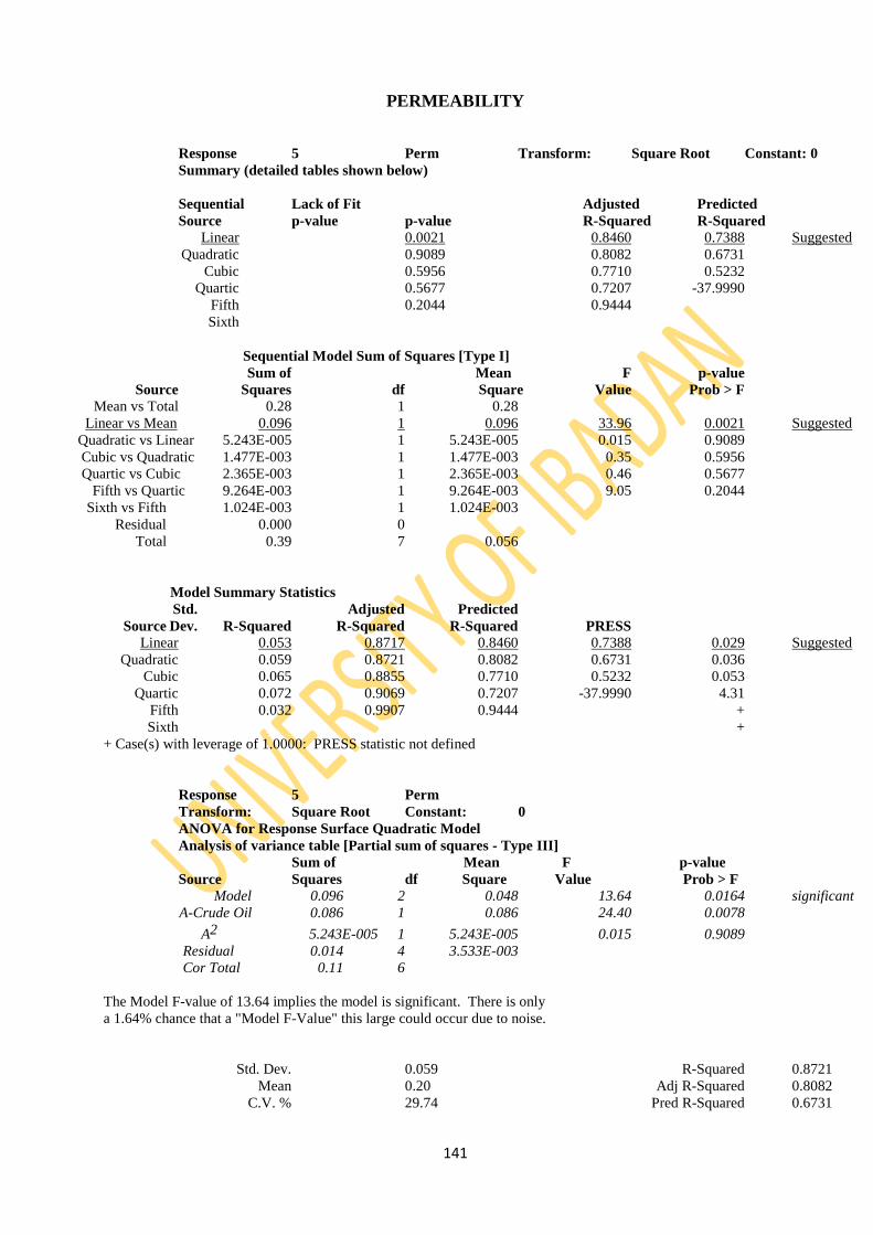
141
PERMEABILITY
Response 5 Perm Transform: Square Root Constant: 0
Summary (detailed tables shown below)
Sequential Lack of Fit Adjusted Predicted
Source p-value p-value R-Squared R-Squared Linear 0.0021 0.8460 0.7388 Suggested
Quadratic 0.9089 0.8082 0.6731
Cubic 0.5956 0.7710 0.5232
Quartic 0.5677 0.7207 -37.9990
Fifth 0.2044 0.9444
Sixth
Sequential Model Sum of Squares [Type I]
Sum of Mean F p-value
Source Squares df Square Value Prob > F Mean vs Total 0.28 1 0.28
Linear vs Mean 0.096 1 0.096 33.96 0.0021 Suggested
Quadratic vs Linear 5.243E-005 1 5.243E-005 0.015 0.9089
Cubic vs Quadratic 1.477E-003 1 1.477E-003 0.35 0.5956
Quartic vs Cubic 2.365E-003 1 2.365E-003 0.46 0.5677
Fifth vs Quartic 9.264E-003 1 9.264E-003 9.05 0.2044
Sixth vs Fifth 1.024E-003 1 1.024E-003
Residual 0.000 0
Total 0.39 7 0.056
Model Summary Statistics
Std. Adjusted Predicted
Source Dev. R-Squared R-Squared R-Squared PRESS Linear 0.053 0.8717 0.8460 0.7388 0.029 Suggested
Quadratic 0.059 0.8721 0.8082 0.6731 0.036
Cubic 0.065 0.8855 0.7710 0.5232 0.053
Quartic 0.072 0.9069 0.7207 -37.9990 4.31
Fifth 0.032 0.9907 0.9444 +
Sixth +
+ Case(s) with leverage of 1.0000: PRESS statistic not defined
Response 5 Perm
Transform: Square Root Constant: 0
ANOVA for Response Surface Quadratic Model
Analysis of variance table [Partial sum of squares - Type III]
Sum of Mean F p-value
Source Squares df Square Value Prob > F Model 0.096 2 0.048 13.64 0.0164 significant
A-Crude Oil 0.086 1 0.086 24.40 0.0078
A2 5.243E-005 1 5.243E-005 0.015 0.9089
Residual 0.014 4 3.533E-003
Cor Total 0.11 6
The Model F-value of 13.64 implies the model is significant. There is only
a 1.64% chance that a "Model F-Value" this large could occur due to noise.
Std. Dev. 0.059 R-Squared 0.8721
Mean 0.20 Adj R-Squared 0.8082
C.V. % 29.74 Pred R-Squared 0.6731

142
PRESS 0.036 Adeq Precision 7.986
The "Pred R-Squared" of 0.6731 is in reasonable agreement with the "Adj R-Squared" of 0.8082.
"Adeq Precision" measures the signal to noise ratio. A ratio greater than 4 is desirable. Your
ratio of 7.986 indicates an adequate signal. This model can be used to navigate the design space.
Coefficient Standard 95% CI 95% CI
Factor Estimate df Error Low High VIF Intercept 0.17 1 0.040 0.062 0.29
A-Crude Oil -0.16 1 0.031 -0.24 -0.068 1.14
A2 -6.957E-003 1 0.057 -0.17 0.15 1.14
Final Equation in Terms of Coded Factors:
Sqrt(Perm) = +0.17-0.16 * A -6.957E-003 * A2
Design-Expert® SoftwarePerm
Color points by value ofPerm:
0.15
0
Actual
Pre
dic
ted
Predicted vs. Actual
0.00
0.05
0.10
0.15
0.20
0.00 0.05 0.10 0.15 0.20
SHRINKAGE LINEAR Response 6 S.L Transform: Square Root Constant: 0
Summary (detailed tables shown below)
Sequential Lack of Fit Adjusted Predicted
Source p-value p-value R-Squared R-Squared Linear < 0.0001 0.9686 0.9476 Suggested
Quadratic 0.8721 0.9611 0.9341
Cubic 0.5650 0.9544 0.8532
Quartic 0.4261 0.9542 -6.0660
Fifth 0.0022 1.0000 Suggested
Sixth
Sequential Model Sum of Squares [Type I]
Sum of Mean F p-value
Source Squares df Square Value Prob > F

143
Mean vs Total 0.36 1 0.36
Linear vs Mean 0.020 1 0.020 186.36 < 0.0001
Suggested
Quadratic vs Linear 3.971E-006 1 3.971E-006 0.029 0.8721
Cubic vs Quadratic 6.572E-005 1 6.572E-005 0.42 0.5650
Quartic vs Cubic 1.562E-004 1 1.562E-004 0.98 0.4261
Fifth vs Quartic 3.180E-004 1 3.180E-004 82125.58 0.0022
Suggested
Sixth vs Fifth 3.872E-009 1 3.872E-009
Residual 0.000 0
Total 0.38 7 0.054
Model Summary Statistics
Std. Adjusted Predicted
Source Dev. R-Squared R-Squared R-Squared PRESS Linear 0.010 0.9739 0.9686 0.9476 1.090E-003 Suggested
Quadratic 0.012 0.9741 0.9611 0.9341 1.373E-003
Cubic 0.013 0.9772 0.9544 0.8532 3.055E-003
Quartic 0.013 0.9847 0.9542 -6.0660 0.15
Fifth 6.223E-005 1.0000 1.0000 + Suggested
Sixth +
+ Case(s) with leverage of 1.0000: PRESS statistic not defined
Design-Expert® SoftwareS.L
Color points by value ofS.L:
0.09
0.02
Actual
Pre
dic
ted
Predicted vs. Actual
0.02
0.04
0.06
0.08
0.10
0.02 0.03 0.04 0.05 0.06 0.07 0.08 0.09
RESISTIVITY
Response 7 Resist Transform: None
Summary (detailed tables shown below)
Sequential Lack of Fit Adjusted Predicted
Source p-value p-value R-Squared R-Squared Linear 0.0048 0.7876 0.6638 Suggested
Quadratic 0.5373 0.7616 0.5523
Cubic 0.9391 0.6829 -2.6999

144
Quartic 0.1385 0.8774 -13.8967
Fifth 0.3007 0.9492
Sixth

145
Sequential Model Sum of Squares [Type I]
Sum of Mean F p-value
Source Squares df Square Value Prob > F Mean vs Total 5800.32 1 5800.32
Linear vs Mean 31.73 1 31.73 23.25 0.0048 Suggested
Quadratic vs Linear 0.70 1 0.70 0.45 0.5373
Cubic vs Quadratic 0.014 1 0.014 6.881E-003 0.9391
Quartic vs Cubic 4.54 1 4.54 5.76 0.1385
Fifth vs Quartic 1.25 1 1.25 3.83 0.3007
Sixth vs Fifth 0.33 1 0.33
Residual 0.000 0
Total 5838.87 7 834.12
Model Summary Statistics
Std. Adjusted Predicted
Source Dev. R-Squared R-Squared R-Squared PRESS Linear 1.17 0.8230 0.7876 0.6638 12.96 Suggested
Quadratic 1.24 0.8411 0.7616 0.5523 17.26
Cubic 1.43 0.8414 0.6829 -2.6999 142.62
Quartic 0.89 0.9591 0.8774 -13.8967 574.22
Fifth 0.57 0.9915 0.9492 +
Sixth +
+ Case(s) with leverage of 1.0000: PRESS statistic not defined
Std. Dev. 1.17 R-Squared 0.8230
Mean 28.79 Adj R-Squared 0.7876
C.V. % 4.06 Pred R-Squared 0.6638
PRESS 12.96 Adeq Precision 8.956
The "Pred R-Squared" of 0.6638 is in reasonable agreement with the "Adj R-Squared" of 0.7876.
Final Equation in Terms of Coded Factors:
Resist =+29.32+2.80 * A
Response 7 Resist Transform: None
Diagnostics Case Statistics
Internally Externally Influence on
Standard Actual Predicted Studentized Studentized Fitted Value Cook's Run
Order Value Value Residual Leverage Residual Residual DFFITS Distance Order 1 31.81 31.00 0.81 0.297 0.831 0.800 0.520 0.146 6
2 28.66 29.88 -1.22 0.180 -1.152 -1.203 -0.564 0.146 5
3 25.07 26.52 -1.45 0.304 -1.492 -1.792 -1.184 0.486 1
4 28.05 26.65 1.40 0.287 1.423 1.650 1.047 0.408 3
5 27.22 26.58 0.64 0.296 0.654 0.611 0.397 0.090 2
6 28.38 28.76 -0.38 0.143 -0.352 -0.318 -0.130 0.010 4
7 32.31 32.11 0.20 0.492 0.234 0.211 0.208 0.027 7
Current Transform: None
Box-Cox Power Transformation
Constant 95% CI 95% CI Best Rec.
k Low High LambdaTransform 0.000 -4.87 9.57 2.35 None

146
Design-Expert® SoftwareResist
Color points by value ofResist:
32.31
25.07
Actual
Pre
dic
ted
Predicted vs. Actual
24.00
26.00
28.00
30.00
32.00
34.00
24.00 26.00 28.00 30.00 32.00 34.00