Effect of corruption on educational quantity and quality

HAL Id: hal-03194726https://hal.uca.fr/hal-03194726

Preprint submitted on 9 Apr 2021

HAL is a multi-disciplinary open accessarchive for the deposit and dissemination of sci-entific research documents, whether they are pub-lished or not. The documents may come fromteaching and research institutions in France orabroad, or from public or private research centers.

L’archive ouverte pluridisciplinaire HAL, estdestinée au dépôt et à la diffusion de documentsscientifiques de niveau recherche, publiés ou non,émanant des établissements d’enseignement et derecherche français ou étrangers, des laboratoirespublics ou privés.

Effect of corruption on educational quantity and quality :theory and evidence

Amadou Boly, Kole Keita, Assi Okara, Guei Okou

To cite this version:Amadou Boly, Kole Keita, Assi Okara, Guei Okou. Effect of corruption on educational quantity andquality : theory and evidence. 2021. �hal-03194726�

https://hal.uca.fr/hal-03194726

https://hal.archives-ouvertes.fr

C E N T R E D ' É T U D E S E T D E R E C H E R C H E S S U R L E D E V E L O P P E M E N T I N T E R N A T I O N A L

SÉRIE ÉTUDES ET DOCUMENTS

Effect of Corruption on Educational Quantity and Quality: Theory and Evidence

Amadou Boly

Kole Keïta Assi Okara

Guei C. Okou

Études et Documents n°16

April 2021

To cite this document:

Boly A., Keïta K., Okara A., Okou G.C. (2021) “Effect of Corruption on Educational Quantity and Quality: Theory and Evidence”, Études et Documents, n°16, CERDI.

CERDI POLE TERTIAIRE 26 AVENUE LÉON BLUM F- 63000 CLERMONT FERRAND TEL. + 33 4 73 17 74 00 FAX + 33 4 73 17 74 28 http://cerdi.uca.fr/

http://cerdi.uca.fr/

Études et Documents n°16, CERDI, 2021

2

The authors Amadou Boly Special assistant, Office of the Chief Economist & Vice President, African Development Bank (AFD), Abidjan, Côte d’Ivoire Email address : [email protected] Kole Keïta Lecturer, Département de Mathématiques Physique Chimie Informatique, Unité de Formation et de Recherche (UFR), Univeristé Jean Lorougnon Guédé, Daloa, Côte d’Ivoire Email address : [email protected] Assi Okara PhD candidate, Université Clermont Auvergne, CNRS, CERDI, F-63000 Clermont-Ferrand, France Email address : [email protected] Guei C. Okou Lecturer, Département de Mathématiques Physique Chimie Informatique, Unité de Formation et de Recherche (UFR), Univeristé Jean Lorougnon Guédé, Daloa, Côte d’Ivoire Email address : [email protected] Corresponding author: Assi Okara

This work was supported by the LABEX IDGM+ (ANR-10-LABX-14-01) within the program “Investissements d’Avenir” operated by the French National Research Agency (ANR).

Études et Documents are available online at: https://cerdi.uca.fr/etudes-et-documents/ Director of Publication: Grégoire Rota-Graziosi Editor: Catherine Araujo-Bonjean Publisher: Aurélie Goumy ISSN: 2114 - 7957 Disclaimer:

Études et Documents is a working papers series. Working Papers are not refereed, they constitute research in progress. Responsibility for the contents and opinions expressed in the working papers rests solely with the authors. Comments and suggestions are welcome and should be addressed to the authors.

mailto:[email protected]





3

Abstract Human capital development, through education and skill development, is instrumental for economic growth. And education and skills development require learning efforts. In the presence of corruption however, applicants have little incentive to learn as they can pass an exam or obtain a qualification by relying on bribery instead. In this paper, we present a simple model with corrupt and honest examiners, as well as applicants with heterogeneous innate ability. A key assumption is that effort and bribe are explicitly modelled as strategic substitutes. Our results show that “strong” candidates rely only upon effort; “medium” candidates choose positive levels of both bribe and effort, while “weak” candidates rely only on bribery. We also find that corruption may decrease education quality by lowering aggregate effort level, while increasing education quantity by increasing the aggregate chances of obtaining a degree. We explore these implications empirically and find support for the key predictions of the model. Keywords

Bribery, Effort, Education JEL Codes

D73, I21, O15


4

1. Introduction

Whether corruption has positive or negative effects on welfare has been a major theoretical

debate in the corruption literature. The positive or “grease-in-the-wheel” view suggested that

corruption may help overcome systemic governmental inefficiencies and distortions, through

simple transfer from firms or individuals to corrupt officials (Leff, 1964; Huntington, 1968;

Leys, 1970; or Lui, 1985). In contrast, the “sand-in-the-wheel” strand argued that, given

officials’ degree of discretionary power, corruption can lead to the creation of

counterproductive regulations to extract more bribes, thereby reducing efficiency and welfare

(Banerjee, 1997; Ades and Di Tella, 1999; Guriev, 2004).1

Available evidence tends to support the “sand-in-the-wheel” view, and corruption is now

widely acknowledged as a major obstacle to economic and social development. Indeed,

corruption has been found to negatively affect growth (Mauro, 1995, 1997; Kaufmann and

Kraay, 2002; Méon and Sekkat, 2005; Swaleheen, 2011); deny government tax revenues

(Friedman, 2000); and cause misallocations of public expenditures (Mauro, 1997; Tanzi and

Davoodi, 1997; Mironov and Zhuravskaya, 2012), lowering in particular the quantity and

quality of health care and educational services (Gupta et al., 2000). Corruption has also been

found to discourage domestic investments (Gyimah-Brempong, 2002) as well as foreign

investments (Wei, 2000; Smarzynska and Wei, 2000; Castro and Nunes, 2013).

In the basic bribery situation, an agent exploits his discretionary power for private gain. For

instance, in exchange for a bribe, an official can lower tax burden or allocate a license to an

undeserving firm (e.g., Amir and Burr, 2015). In the latter case, corruption substitutes itself for

or undermine qualification (Drugov, 2010) or a capacitating activity, such as learning and skill

building. This is particularly so in the education sector, our focus, where effort and learning are

required to build human capital, pass an exam, or obtain a degree; and student time and

engagement may be considered the single most important input in the educational process

(Bishop, 1996). But clearly, corruption may substitute itself for learning effort, and anecdotal

evidence abounds. For instance, in 2014, an audit of the 2011 entrance examination at the Ecole

Normale Supérieure in Cote d’Ivoire revealed that 23 candidates who never sat the exam were

1 For instance, to attract bribes, the official could reduce the number of licences to allocate, be overzealous in his tax collection effort, or delay unnecessarily the production of an official document.


5

admitted. An applicant was ranked 3rd while actual ranking was 724th; another one was ranked

6th while actual ranking was 185th. 2

Corruption in the education sector may have serious economic implications.3 Education, as

part of human capital, has been shown to have a positive effect on growth (Hanushek and

Kimko, 2000; Barro, 2001). Yet, corruption can weaken incentives to work hard and acquire

skills, thereby negatively impacting growth. Corruption in education can also affect the labour

markets if firms only observe educational attainment but not the level of skills acquired

(Costrell, 1994; Betts, 1998). In this case, the expected level of productivity conditional on

graduating may be lower in the presence of corruption, leading to a lower level of wage (see

e.g., Heyneman, Anderson, and Nuraliyeva, 2008).

A small literature explores specifically the link between education and corruption. Ehrlich

and Lui (1999) showed that corruption affects economic growth by diverting resources from

human capital formation towards non-productive rent-seeking activities (political capital).

Eicher et al. (2009) analyzed the interplay between education, corruption (embezzlement of

public funds) and growth. They showed that education increases the rents obtained by a corrupt

politician, but also the probability of being identified as corrupt and not being reelected.

Corruption in turn affects investment in education by lowering income level. In contrast to these

earlier studies, this paper examines how corruption may undermine the learning process at the

root, by altering individuals’ incentives to invest in education.

Our model is as follows. To obtain a qualification or pass an exam, valued at V,

heterogeneous risk-neutral applicants have to pass a test, optimally choosing between learning

effort and bribery to maximize their utility.4 Applicants’ heterogeneity is modelled as a

difference in innate ability, denoted 𝛽𝛽. There are two types of officials: honest or corrupt. The

types are determined by nature. For simplicity, honest officials take only learning effort (effort

hereafter) into account in measuring the candidate’s performance, while corrupt officials care

only about the bribe size. Both effort and bribery positively contribute to the candidate’s

probability of success, but are costly. A key assumption in our model is that effort and bribe are

explicitly modelled as strategic substitutes; and there is no detection probability or sanction.

2 See http://www.civox.net/Ecole-Nationale-de-l-Administration-Toute-la-verite-sur-les-fraudes-a-l-ENA_a5867.html 3 For reviews of corruption in academe, see Heyneman (2004) and Rumyantseva (2005). 4 In our model, bribery may be interpreted as any kind of effort not directed at learning and with the objective to obtain some favour or influence. So our definition of bribery goes beyond monetary payments (see Clark and Riis 2000).

http://www.civox.net/Ecole-Nationale-de-l-Administration-Toute-la-verite-sur-les-fraudes-a-l-ENA_a5867.html

http://www.civox.net/Ecole-Nationale-de-l-Administration-Toute-la-verite-sur-les-fraudes-a-l-ENA_a5867.html


6

Our results show behavioural heterogeneity regarding candidates’ optimal choices of effort

and bribe (see Fender, 1999). The “strong” candidates rely only on effort; “medium” candidates

choose positive levels of both bribe and effort, while “weak” candidates rely only on bribery.

Such behavioural differences result in inefficiencies, as the best candidates would fail if they

encounter a corrupt official; while weak candidates may still succeed through bribery. Such a

result is closest to Ahlin and Bose (2007) who, in a dynamic setting, showed that in the presence

of honest officials and the opportunity to re-apply for a permit, efficient applicants have a lower

willingness to pay a bribe and prefer to wait until the next period while inefficient applicants

pay the bribe in the first period. As a result, the inefficient type is serviced ahead of the efficient

one, which may even never be serviced.

By aggregating heterogeneous individual decisions into “economy-wide” effort level or

expected rate of success, we provide a simple channel through which micro-level corruption

decisions may translate into macro-economic effects, potentially impeding economic and social

development.5 Specifically, effort level or expected rate of success could be interpreted as

education quality and education quantity respectively. Our results suggest that corruption may

decrease education quality, as a higher proportion of corrupt officials lowers aggregate effort

level and increases the proportion of candidates choosing to exert no effort at all. On the other

hand, corruption may increase education quantity by increasing the chances of obtaining a

degree, even without effort.

Although we focus on the education sector, our analysis has a more general applicability as

it extends to most situations where corruption substitutes itself for learning and skill building

to attain the desired goal. For instance, before obtaining a driver license, it is necessary to pass

both a knowledge and a road test. If corruption may be used instead of effort to obtain a driver

license (e.g., Bertrand et al., 2006), more unsafe drivers may be put on the road, which may

translate into a higher number of road accidents or deaths. Likewise, firms are typically required

to invest into satisfying some requirements before being eligible for certain licenses. In the

presence of corruption, firms can buy these licenses rather than investing, possibly imposing

negative externalities on society.

5 One characteristic of the corruption literature is that most theoretical studies of corruption are micro-models, while empirical studies focus on cross-country analyses, leaving a gap between these two approaches to study corruption.


7

2. The Benchmark Case

We start by presenting a model without corruption before turning to the case with corruption.

Our model builds on De Paola and Scoppa (2007). In this model, applicants are risk neutral

with utility function:

𝑈𝑈(𝑒𝑒, 𝛽𝛽) = 𝑃𝑃𝑃𝑃(𝑆𝑆 = 1) 𝑉𝑉 − 𝑐𝑐(𝑒𝑒) = 𝛽𝛽𝑒𝑒𝑉𝑉 −12

𝑒𝑒2

This utility function is derived as follows. To obtain a qualification or pass an exam, valued

at 𝑉𝑉 Є [0,1], heterogeneous risk-neutral applicants have to pass a test, by choosing a learning

effort level 𝑒𝑒; which also denotes the skill level acquired in the learning process. Applicants are

characterized by their innate ability β, uniformly distributed on [0, 1]. In this section, we assume

that the examiners are all honest, meaning that only 𝑒𝑒 is taken into account in performance

evaluation. A candidate’s performance, denoted s, therefore depends only on effort 𝑒𝑒 and innate

ability β such that:

𝑠𝑠 = 𝛽𝛽𝑒𝑒.

The final performance is given by 𝑠𝑠 − 𝜀𝜀, indicating that performance is measured with

error 𝜀𝜀, uniformly distributed on the interval [0, 1]. To pass an exam, performance must be

higher or equal to a given threshold, here zero (𝑠𝑠 − 𝜀𝜀 ≥ 0). We define S a random variable

which is equal to 1 if an applicant is successful in passing an exam; and 0 otherwise:

� 𝑆𝑆 = 1 𝑖𝑖𝑖𝑖 𝑠𝑠 − 𝜀𝜀 ≥ 0 𝑆𝑆 = 0 otherwise

An applicant therefore passes his/her exam with probability:

𝑃𝑃𝑃𝑃(𝑆𝑆 = 1) = 𝑃𝑃𝑃𝑃(𝑠𝑠 − 𝜀𝜀 ≥ 0) = 𝑃𝑃(𝑠𝑠 ≥ 𝜀𝜀) = ∫ 𝑑𝑑𝜀𝜀𝑠𝑠0 = 𝛽𝛽𝑒𝑒 .

The partial derivative relative to effort is: 𝜕𝜕𝜕𝜕𝜕𝜕(𝑆𝑆=1)𝜕𝜕𝜕𝜕

= 𝛽𝛽 ≥ 0 , indicating that the probability

of success is increasing in effort level. However, it is worth noting that effort exerted by a

candidate increases chances of success but does not guarantee it. Likewise, the partial derivative

relative to innate ability β is: 𝜕𝜕𝜕𝜕𝜕𝜕(𝑆𝑆=1)𝜕𝜕𝜕𝜕

= 𝑒𝑒 ≥ 0, suggesting that the probability of success

increases with ability.


8

The cost function of effort is given by 𝑐𝑐(𝑒𝑒) = 12

𝑒𝑒2. This function is increasing and convex

since 𝑐𝑐′(𝑒𝑒) = 𝑒𝑒 ≥ 0 and 𝑐𝑐′′(𝑒𝑒) = 1.

The optimal value of effort is given by 𝜕𝜕𝜕𝜕(𝜕𝜕,𝜕𝜕)𝜕𝜕𝜕𝜕

= 0 ⟹ 𝑒𝑒∗ = 𝛽𝛽𝑉𝑉.

Optimal effort is monotonically increasing in applicants’ innate ability 𝛽𝛽 and in the value

of 𝑉𝑉. All types of applicants exert a positive amount of effort except the lowest type whose

optimal effort level is 0. The aggregate effort is given by:

𝐸𝐸(𝑒𝑒∗) = � 𝑒𝑒∗𝑖𝑖(𝛽𝛽)𝑑𝑑𝛽𝛽1

0

= � 𝛽𝛽𝑉𝑉𝑖𝑖(𝛽𝛽)𝑑𝑑𝛽𝛽 = 𝑉𝑉 � 𝛽𝛽𝑑𝑑𝛽𝛽 =𝑉𝑉2

1

0

1

0

.

The aggregate probability of success is given by:

𝐸𝐸(𝑆𝑆 = 1|0 ≤ 𝛽𝛽 ≤ 1) = 𝐸𝐸(𝜀𝜀 ≤ 𝛽𝛽e∗ |0 ≤ 𝛽𝛽 ≤ 1) = � 𝜀𝜀 𝑖𝑖𝜀𝜀|0≤𝜕𝜕≤1(𝜀𝜀)

𝜕𝜕e∗

0

dε

= � 𝜀𝜀 𝑖𝑖(𝜀𝜀, 0 ≤ 𝛽𝛽 ≤ 1)𝑖𝑖(0 ≤ 𝛽𝛽 ≤ 1)

𝜕𝜕e∗

0

dε = � 𝜀𝜀 𝑖𝑖(𝜀𝜀, 0 ≤ 𝛽𝛽 ≤ 1)

𝜕𝜕e∗

0

dε = � 𝜀𝜀

𝜕𝜕e∗

0

dε = 𝛽𝛽2e∗2

2

= 𝛽𝛽4𝑉𝑉2

2.

3. The Case with Corruption

Now, among the examiners, we assume that there exists a proportion θ that is corrupt and (1-θ)

that is honest. Officials’ types are private information but θ is common knowledge.6 As in the

previous section, applicants are characterized by their innate ability β, uniformly distributed on

[0,1]. To obtain a qualification, a candidate chooses between effort 𝑒𝑒, bribe 𝑏𝑏, or a combination.

In this case, final performance is measured as 𝑠𝑠 − 𝜀𝜀 = (1 − 𝜃𝜃)𝛽𝛽𝑒𝑒 + 𝜃𝜃𝑏𝑏 − 𝜀𝜀 where the error ε

is uniformly distributed on [0, 1].

The probability of success of a candidate is given by

𝑃𝑃(𝑆𝑆 = 1) = 𝑃𝑃(𝑠𝑠 − 𝜀𝜀 ≥ 0) = (1 − 𝜃𝜃)𝛽𝛽𝑒𝑒 + 𝜃𝜃𝑏𝑏

6 This assumption denotes the presence of intrinsically motivated agents that resist corruption (see e.g. Ahlin and Bose 2007).


9

This probability of success increases with innate ability, effort and bribe because

𝜕𝜕𝜕𝜕(𝑆𝑆=1)𝜕𝜕𝜕𝜕

≥0, 𝜕𝜕𝜕𝜕(𝑆𝑆=1)𝜕𝜕𝜕𝜕

≥0 and 𝜕𝜕𝜕𝜕(𝑆𝑆=1)𝜕𝜕𝜕𝜕

≥0.

The cost function is given by:

𝐶𝐶(𝑒𝑒, 𝑏𝑏) = 12

(𝑒𝑒2 + 𝑏𝑏2) + 𝑘𝑘𝑒𝑒𝑏𝑏 where 𝑘𝑘 ∈ [0, 1].

This cost function assumes that effort and bribery are strategic substitutes and 𝑘𝑘 is a measure

of the degree of substitutability.7 An increase in the level of effort increases the marginal cost

of bribe and vice-versa. As a result, a risk neutral applicant’s utility function is given by:

𝑈𝑈(𝑒𝑒, 𝑏𝑏, 𝛽𝛽) = 𝑃𝑃(𝑆𝑆 = 1)𝑉𝑉 − 𝐶𝐶(𝑒𝑒, 𝑏𝑏) = �(1 − 𝜃𝜃)𝛽𝛽𝑒𝑒 + 𝜃𝜃𝑏𝑏�𝑉𝑉 − 12

(𝑒𝑒2 + 𝑏𝑏2) − 𝑘𝑘𝑒𝑒𝑏𝑏

The applicant chooses effort 𝑒𝑒 and bribe 𝑏𝑏 in order to maximize this utility function.

Optimal Behavior

Let 𝜆𝜆 (resp µ) be the Lagrange multipliers associated to 𝑒𝑒 (resp 𝑏𝑏 ). The Lagrangian is

given by:

𝐿𝐿(𝑒𝑒, 𝑏𝑏, 𝜆𝜆, µ) = �(1 − 𝜃𝜃)𝛽𝛽𝑒𝑒 + 𝜃𝜃𝑏𝑏�𝑉𝑉 − 12

(𝑒𝑒2 + 𝑏𝑏2) − 𝑘𝑘𝑒𝑒𝑏𝑏 + 𝜆𝜆𝑒𝑒 + 𝜇𝜇𝑏𝑏.

The Lagrangian is a concave function. So, using Karush-Kuhn-Tucker (KKT) sufficient

conditions, we find the following:

�𝛻𝛻𝐿𝐿(𝑒𝑒, 𝑏𝑏, 𝜆𝜆, µ) = 0

𝑒𝑒 ≥ 0, 𝑏𝑏 ≥ 0, 𝜆𝜆 ≥ 0,𝜆𝜆𝑒𝑒 = 0, 𝜇𝜇𝑏𝑏 = 0

µ ≥ 0

⟹ �(1 − 𝜃𝜃)𝛽𝛽𝑉𝑉 − 𝑒𝑒 − 𝑘𝑘𝑏𝑏 + 𝜆𝜆 = 0, 𝜃𝜃𝑉𝑉 − 𝑏𝑏 − 𝑘𝑘𝑒𝑒 + 𝜇𝜇 = 0

𝑒𝑒 ≥ 0, 𝑏𝑏 ≥ 0, 𝜆𝜆 ≥ 0, µ ≥ 0𝜆𝜆𝑒𝑒 = 0, 𝜇𝜇𝑏𝑏 = 0

By resolving the first equations, for 𝑘𝑘 ≠ 1 we obtain:

7 See Dixit (2002) for such a modelling of substitutable tasks, with actions interacting in the cost, but not in the production function. If 𝑘𝑘 = 0, effort and bribery are independent, while if 𝑘𝑘 = 1, they are perfect substitutes.


10

𝑒𝑒∗ =

�(1 − 𝜃𝜃)𝛽𝛽 − 𝑘𝑘𝜃𝜃�𝑉𝑉1 − 𝑘𝑘2 +

𝜆𝜆1 − 𝑘𝑘2 −

𝑘𝑘𝜇𝜇1 − 𝑘𝑘2 ,

𝑏𝑏∗ =(𝜃𝜃 − 𝑘𝑘(1 − 𝜃𝜃)𝛽𝛽)𝑉𝑉

1 − 𝑘𝑘2 −𝑘𝑘𝜆𝜆

1 − 𝑘𝑘2 +𝜇𝜇

1 − 𝑘𝑘2.

We will now discuss the various solutions by analyzing different cases:

Case 1 2 3 4

𝒆𝒆∗ 0 �(1−𝜃𝜃)𝜕𝜕−𝑘𝑘𝜃𝜃�𝑉𝑉1−𝑘𝑘2 0 (1 − 𝜃𝜃)𝛽𝛽𝑉𝑉

𝒃𝒃∗ 0 (𝜃𝜃−𝑘𝑘(1−𝜃𝜃)𝜕𝜕)𝑉𝑉1−𝑘𝑘2 𝜃𝜃𝑉𝑉 0

𝝀𝝀∗ −(1 − 𝜃𝜃)𝛽𝛽𝑉𝑉 0 (𝑘𝑘𝜃𝜃 − (1 − 𝜃𝜃)𝛽𝛽)𝑉𝑉 0

𝝁𝝁∗ −𝜃𝜃𝑉𝑉 0 0 (𝑘𝑘(1 − 𝜃𝜃)𝛽𝛽 − 𝜃𝜃)𝑉𝑉

Proposition 1: The optimal levels of bribe and effort result in a probability success

𝑃𝑃(𝑆𝑆 = 1) Є [0,1].

Proof:

Case 1 can be excluded since the non-negativity constraints of the Lagrange multipliers would

be violated.

In case 2, e∗ > 0 and 𝑏𝑏∗ > 0 , then 𝑒𝑒∗ + 𝑏𝑏∗ = (𝜃𝜃+(1−𝜃𝜃)𝜕𝜕)𝑉𝑉 𝑘𝑘+1

.

We have 𝜃𝜃 + (1 − 𝜃𝜃)𝛽𝛽 as a convex combination of 𝛽𝛽 and 1 (this combination is inferior

or equal to 1 because β ≤ 1 and 0 ≤ 𝑉𝑉𝑘𝑘+1

≤ 1) . So, if 0 ≤ 𝑒𝑒∗ + 𝑏𝑏∗ ≤ 1, then 0 ≤

(1 − 𝜃𝜃)𝛽𝛽𝑒𝑒∗ + 𝜃𝜃𝑏𝑏∗ ≤ 1 as a convex combination, noting that 𝑃𝑃(𝑆𝑆 = 1) = (1 − 𝜃𝜃)𝛽𝛽𝑒𝑒 + 𝜃𝜃𝑏𝑏.

The optimal solution is 𝑒𝑒∗ = �(1−𝜃𝜃)𝜕𝜕−𝑘𝑘𝜃𝜃�𝑉𝑉1−𝑘𝑘2 and 𝑏𝑏∗ = (𝜃𝜃−𝑘𝑘(1−𝜃𝜃)𝜕𝜕)𝑉𝑉

1−𝑘𝑘2 . The applicant exerts

some effort in addition to bribery in order to obtain her qualification. This situation resembles

the case where an applicant obtains the exams but not the solutions (see Tucker 2000).

Partially differentiating 𝑒𝑒∗ and 𝑏𝑏∗ with respect to 𝜃𝜃 gives:

𝜕𝜕𝜕𝜕∗

𝜕𝜕𝜃𝜃= − (𝜕𝜕+𝑘𝑘)𝑉𝑉

1−𝑘𝑘2 ≤ 0 and 𝜕𝜕𝜕𝜕∗

𝜕𝜕𝜃𝜃= (1+𝑘𝑘𝜕𝜕)𝑉𝑉

1−𝑘𝑘2 ≥ 0, or all 𝑘𝑘 Є [0,1[.

The graphs below depict the evolution of optimal effort and bribe according to the

proportion of corrupt examiners.


11

Figure 1: Evolution of the optimal effort (blue curve) and optimal bribe (black curve)

according to the proportion of corrupt examiners.

Note: The curves are represented with k = 1

2 . The curves correspond to the evolutions of the optimal values

according to the proportion of corrupt examiners θ. The variations of optimal values depend on the selected values of innate ability β and qualification V. The amplitudes of optimal values depend on V. In summary, optimal values of effort and bribe are proportionally linear in qualification V, but the slopes of the curves depend on innate ability. The curves show that 𝑒𝑒∗ decreases with θ while 𝑏𝑏∗ increases.

Partially differentiating 𝑒𝑒∗ and 𝑏𝑏∗ with respect to 𝛽𝛽 gives:

𝜕𝜕𝜕𝜕∗

𝜕𝜕𝜕𝜕= (1−𝜃𝜃)𝑉𝑉

1−𝑘𝑘2 ≥ 0 and 𝜕𝜕𝜕𝜕∗

𝜕𝜕𝜕𝜕= − 𝑘𝑘(1−𝜃𝜃)𝑉𝑉

1−𝑘𝑘2 ≤ 0 for all 𝑘𝑘 Є [0,1[ . This implies that optimal

effort increases in innate ability β while the optimal bribe decreases with β.

Partially differentiating 𝑒𝑒∗ and 𝑏𝑏∗ with respect to V gives:

𝜕𝜕𝜕𝜕∗

𝜕𝜕𝑉𝑉= �(1−𝜃𝜃)𝜕𝜕−𝑘𝑘𝜃𝜃�

1−𝑘𝑘2 and 𝜕𝜕𝜕𝜕∗

𝜕𝜕𝑉𝑉= (𝜃𝜃−𝑘𝑘(1−𝜃𝜃)𝜕𝜕)

1−𝑘𝑘2 . These variations of ∂e∗

∂V and ∂b∗

∂V depend on the

innate ability value 𝛽𝛽.

If we suppose that 𝛽𝛽 + 𝑘𝑘 ≠ 0, then:


12

• for all 𝜃𝜃 Є [0, 𝜕𝜕𝜕𝜕+𝑘𝑘

], 𝜕𝜕𝜕𝜕∗

𝜕𝜕𝑉𝑉≥ 0 ⟹ 𝑒𝑒∗ increases according to the qualification.

• for all 𝜃𝜃 Є [ 𝜕𝜕𝜕𝜕+𝑘𝑘

, 1], 𝜕𝜕𝜕𝜕∗

𝜕𝜕𝑉𝑉≤ 0 ⟹ 𝑒𝑒∗ decreases according to the qualification.

For the variation of bribe with respect to the qualification, we have:

• for all 𝜃𝜃 Є [0, 𝑘𝑘𝜕𝜕1+𝑘𝑘𝜕𝜕

], 𝜕𝜕𝜕𝜕∗

𝜕𝜕𝑉𝑉≤ 0 ⟹ 𝑏𝑏∗ decreases according to the qualification.

• for all 𝜃𝜃 Є [ 𝑘𝑘𝜕𝜕1+𝑘𝑘𝜕𝜕

, 1], 𝜕𝜕𝜕𝜕∗

𝜕𝜕𝑉𝑉≥ 0 ⟹ 𝑏𝑏∗ increase according to the qualification.

In case 3, the optimal solution is 𝑒𝑒∗ = 0 and 𝑏𝑏∗ = 𝜃𝜃𝑉𝑉. The applicant exerts no effort to obtain

her degree and relies solely upon bribery. Using Tucker (2000)’s example, this can correspond

to the case where the applicant obtains the exams and the solutions. Applicants pay a fixed price

whenever they do not exert any effort, and 𝑏𝑏∗ in this case is independent of innate ability 𝛽𝛽.

In case 4, the optimal solution is 𝑒𝑒∗ = (1 − 𝜃𝜃)𝛽𝛽𝑉𝑉 and 𝑏𝑏∗ = 0. The applicant does not resort

to bribery to get the degree or pass an exam. This coincides with the case where the applicant

does not try to obtain either the exams or the solutions. The level of effort is decreasing in the

proportion of corrupt officials and increasing in ability.

Using the results of case 2, it is possible to find the values of 𝛽𝛽 that makes an individual

indifferent between 𝑒𝑒∗ = 0 and 𝑒𝑒∗ = �(1−𝜃𝜃)𝜕𝜕−𝑘𝑘𝜃𝜃�𝑉𝑉1−𝑘𝑘2 , or between 𝑏𝑏∗ = 0 and 𝑏𝑏∗ = (𝜃𝜃−𝑘𝑘(1−𝜃𝜃)𝜕𝜕)𝑉𝑉

1−𝑘𝑘2 .

The results are summarized in the following proposition.

Proposition 2: There exists a threshold 𝛽𝛽𝑙𝑙 = 𝑘𝑘𝜃𝜃(1−𝜃𝜃)

such that for all 𝛽𝛽 ∈ [0, 𝛽𝛽𝑙𝑙], a candidate

does not exert any effort in order to obtain qualification. There also exists a threshold 𝛽𝛽ℎ =𝜃𝜃

𝑘𝑘(1−𝜃𝜃) such that for all 𝛽𝛽 ∈ [𝛽𝛽ℎ, 1], a candidate relies solely on effort in order to obtain

qualification. For 𝛽𝛽 ∈ [𝛽𝛽𝑙𝑙, 𝛽𝛽ℎ], a candidate uses both effort and bribery to get their

qualifications 𝑒𝑒∗ = �(1−𝜃𝜃)𝜕𝜕−𝑘𝑘𝜃𝜃�𝑉𝑉1−𝑘𝑘2 and 𝑏𝑏∗ = (𝜃𝜃−𝑘𝑘(1−𝜃𝜃)𝜕𝜕)𝑉𝑉

1−𝑘𝑘2 .

Proof:

𝛽𝛽𝑙𝑙 is obtained using 𝑒𝑒∗ = �(1−𝜃𝜃)𝜕𝜕−𝑘𝑘𝜃𝜃�𝑉𝑉1−𝑘𝑘2 = 0, giving:

(1 − 𝜃𝜃) 𝛽𝛽𝑙𝑙 − 𝑘𝑘𝜃𝜃 = 0 ⇔ 𝛽𝛽𝑙𝑙 = 𝑘𝑘𝜃𝜃(1−𝜃𝜃) , assuming 𝜃𝜃 Є [0,1[.


13

𝛽𝛽ℎ is obtained in a similar way by equalizing 𝑏𝑏∗ = 0 where 𝑏𝑏∗ = (𝜃𝜃−𝑘𝑘(1−𝜃𝜃)𝜕𝜕)𝑉𝑉1−𝑘𝑘2 with 𝑉𝑉 ≠ 0.

Then 𝜃𝜃 − 𝑘𝑘(1 − 𝜃𝜃)𝛽𝛽ℎ = 0 ⇔ 𝛽𝛽ℎ = 𝜃𝜃𝑘𝑘(1−𝜃𝜃) , assuming 𝜃𝜃 Є [0,1[.

Note that 𝛽𝛽𝑙𝑙 ≤ 𝛽𝛽ℎ. We assume 0 ≤ 𝛽𝛽𝑙𝑙 ≤ 𝛽𝛽ℎ ≤ 1 and 𝜃𝜃 ≤ 𝑚𝑚𝑖𝑖𝑚𝑚 � 𝑘𝑘1+𝑘𝑘

, 11+𝑘𝑘

� = 𝑘𝑘1+𝑘𝑘

. Note

also that when 𝜃𝜃 tends to 11+𝑘𝑘

, then 𝛽𝛽𝑙𝑙 tends to 1 and effort remains zero.

Partially differentiating 𝛽𝛽𝑙𝑙 and 𝛽𝛽ℎ with respect to 𝜃𝜃 gives:

𝜕𝜕𝜕𝜕𝑙𝑙𝜕𝜕𝜃𝜃

= 𝑘𝑘(1−𝜃𝜃)2 ≥ 0 and 𝜕𝜕𝜕𝜕ℎ

𝜕𝜕𝜃𝜃= 1

𝑘𝑘(1−𝜃𝜃)2 ≥ 0 ⟹ 𝛽𝛽𝑙𝑙 is increasing in 𝜃𝜃.

A higher proportion of candidates does not acquire any skill when 𝜃𝜃 increases. As 𝛽𝛽ℎ is

also increasing in 𝜃𝜃, a higher proportion of candidates that was initially relying only on effort,

now substitute effort for bribery.

4. Aggregate Effort

Since effort and bribery are substitutes, an intuitive implication is that a higher proportion of

corrupt officials decreases the expected level of effort exerted by candidates. At the societal

level, this may translate in a lower level of acquired skills, and therefore a lower level of

education quality.

The expected level of effort is given by the expression below:

𝐸𝐸(𝑒𝑒∗) = ∫ 𝑒𝑒∗𝑖𝑖(𝛽𝛽) 𝑑𝑑𝛽𝛽 = ∫ 𝑒𝑒∗𝑖𝑖(𝛽𝛽) 𝑑𝑑𝛽𝛽𝜕𝜕𝑙𝑙0 + ∫ 𝑒𝑒∗ 𝑖𝑖(𝛽𝛽)𝑑𝑑𝛽𝛽𝜕𝜕ℎ

𝜕𝜕𝑙𝑙+ ∫ 𝑒𝑒∗ 𝑖𝑖(𝛽𝛽)𝑑𝑑𝛽𝛽1

𝜕𝜕ℎ

10

= � 0 𝑑𝑑𝛽𝛽

𝜕𝜕𝑙𝑙

0

+ ��(1 − 𝜃𝜃)𝛽𝛽 − 𝑘𝑘𝜃𝜃�𝑉𝑉

1 − 𝑘𝑘2 𝑑𝑑𝛽𝛽

𝜕𝜕ℎ

𝜕𝜕𝑙𝑙

+ �(1 − 𝜃𝜃)𝛽𝛽𝑉𝑉𝑑𝑑𝛽𝛽1

𝜕𝜕ℎ

=𝑉𝑉

1 − 𝑘𝑘2 [ (1 − 𝜃𝜃)𝛽𝛽2

2− 𝑘𝑘𝜃𝜃𝛽𝛽 ]𝜕𝜕𝑙𝑙

𝜕𝜕ℎ + 𝑉𝑉[(1 − 𝜃𝜃)𝛽𝛽2

2 ]𝜕𝜕ℎ

1

= 𝑉𝑉

1 − 𝑘𝑘2 [ (1 − 𝜃𝜃)�𝛽𝛽ℎ

2 − 𝛽𝛽𝑙𝑙2�

2− 𝑘𝑘𝜃𝜃(𝛽𝛽ℎ − 𝛽𝛽𝑙𝑙)] +

𝑉𝑉(1 − 𝜃𝜃)(1 − 𝛽𝛽ℎ2)

2 .

We replace 𝛽𝛽𝑙𝑙 = 𝑘𝑘𝜃𝜃(1−𝜃𝜃)

and 𝛽𝛽ℎ = 𝜃𝜃𝑘𝑘(1−𝜃𝜃)

in the expression above to obtain respectively:


14

𝑘𝑘𝑉𝑉𝜃𝜃1−𝑘𝑘2 (𝛽𝛽ℎ − 𝛽𝛽𝑙𝑙) = 𝑉𝑉𝜃𝜃2

1−𝜃𝜃 , 𝑉𝑉(1−𝜃𝜃)(𝜕𝜕ℎ

2−𝜕𝜕𝑙𝑙2)

2(1−𝑘𝑘2)= 𝑉𝑉𝜃𝜃2(1+𝑘𝑘2)

2𝑘𝑘2(1−𝜃𝜃) and 𝑉𝑉(1−𝜃𝜃)(1−𝜕𝜕ℎ

2)2

= 𝑉𝑉(𝑘𝑘2(1−𝜃𝜃)2−𝜃𝜃2)2𝑘𝑘2(1−𝜃𝜃)

.

As a result, the expected level of effort is given by:

𝐸𝐸(𝑒𝑒∗) = 𝑉𝑉(1−2𝜃𝜃)2(1−𝜃𝜃)

with 𝜕𝜕𝜕𝜕(𝜕𝜕∗)𝜕𝜕𝜃𝜃

= − 𝑉𝑉2(1−𝜃𝜃)2 ≤ 0.

This result suggests that the expected level of effort exerted by applicants decreases with

the proportion of corrupt examiners. Therefore, a higher proportion of corrupt officials can lead

to a lower level of education quality. The expected level of effort converges to the result

obtained in the model of the Benchmark case (not considering the corruption) if the proportion

of corrupt graders tends to zero.

5. Aggregate Rate of Success

In this section, we compute the expected rate of success among applicants in the presence of

corruption. We distinguish three cases according to applicants’ types.

Case 1: 𝜷𝜷 ∈ [𝟎𝟎, 𝜷𝜷𝒍𝒍]

In the presence of corruption, this type of candidate relies solely on bribery. Since an applicant

in this interval chooses 𝑒𝑒∗ = 0 , he will be disqualified by honest officials whose proportion is

(1 − 𝜃𝜃). On the other hand, he may be successful if he encounters a corrupt official, leading to

a first inefficiency result.

Conditional on the official being corrupt, the bribe paid is 𝑏𝑏∗ = 𝜃𝜃 𝑉𝑉. Taking into account

the proportion of corrupt official, we obtain that the probability of success is 𝜃𝜃2 𝑉𝑉. So, the

average probability of success is given by:

𝐸𝐸(𝑆𝑆 = 1|0 ≤ 𝛽𝛽 ≤ 𝛽𝛽𝑙𝑙) = 𝐸𝐸(𝜀𝜀 ≤ 𝜃𝜃2𝑉𝑉|0 ≤ 𝛽𝛽 ≤ 𝛽𝛽𝑙𝑙)

= � 𝜀𝜀 𝑖𝑖(𝜀𝜀, 0 ≤ 𝛽𝛽 ≤ 𝛽𝛽𝑙𝑙)𝑖𝑖(0 ≤ 𝛽𝛽 ≤ 𝛽𝛽𝑙𝑙)

𝑑𝑑𝜀𝜀𝜃𝜃2𝑉𝑉

0

= � 𝜀𝜀 𝑖𝑖(𝜀𝜀, 0 ≤ 𝛽𝛽 ≤ 𝛽𝛽𝑙𝑙)

𝛽𝛽𝑙𝑙𝑑𝑑𝜀𝜀

𝜃𝜃2𝑉𝑉

0

= �𝜀𝜀𝛽𝛽𝑙𝑙

𝑑𝑑𝜀𝜀𝜃𝜃2𝑉𝑉

0

= 𝜃𝜃4

2𝛽𝛽𝑙𝑙𝑉𝑉2.


15

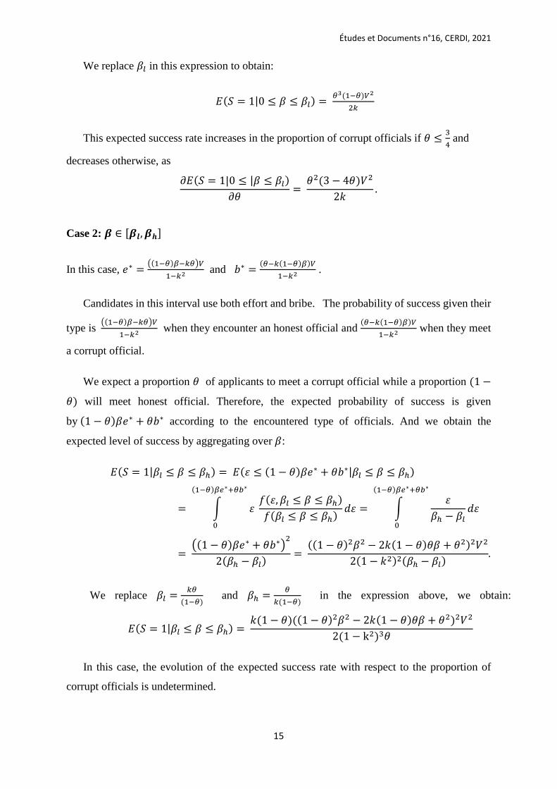
We replace 𝛽𝛽𝑙𝑙 in this expression to obtain:

𝐸𝐸(𝑆𝑆 = 1|0 ≤ 𝛽𝛽 ≤ 𝛽𝛽𝑙𝑙) = 𝜃𝜃3(1−𝜃𝜃)𝑉𝑉2

2𝑘𝑘

This expected success rate increases in the proportion of corrupt officials if 𝜃𝜃 ≤ 34 and

decreases otherwise, as

𝜕𝜕𝐸𝐸(𝑆𝑆 = 1|0 ≤ |𝛽𝛽 ≤ 𝛽𝛽𝑙𝑙)𝜕𝜕𝜃𝜃

= 𝜃𝜃2(3 − 4𝜃𝜃)𝑉𝑉2

2𝑘𝑘.

Case 2: 𝜷𝜷 ∈ [𝜷𝜷𝒍𝒍, 𝜷𝜷𝒉𝒉]

In this case, 𝑒𝑒∗ = �(1−𝜃𝜃)𝜕𝜕−𝑘𝑘𝜃𝜃�𝑉𝑉1−𝑘𝑘2 and 𝑏𝑏∗ = (𝜃𝜃−𝑘𝑘(1−𝜃𝜃)𝜕𝜕)𝑉𝑉

1−𝑘𝑘2 .

Candidates in this interval use both effort and bribe. The probability of success given their

type is �(1−𝜃𝜃)𝜕𝜕−𝑘𝑘𝜃𝜃�𝑉𝑉1−𝑘𝑘2 when they encounter an honest official and (𝜃𝜃−𝑘𝑘(1−𝜃𝜃)𝜕𝜕)𝑉𝑉

1−𝑘𝑘2 when they meet

a corrupt official.

We expect a proportion 𝜃𝜃 of applicants to meet a corrupt official while a proportion (1 −

𝜃𝜃) will meet honest official. Therefore, the expected probability of success is given

by (1 − 𝜃𝜃)𝛽𝛽𝑒𝑒∗ + 𝜃𝜃𝑏𝑏∗ according to the encountered type of officials. And we obtain the

expected level of success by aggregating over 𝛽𝛽:

𝐸𝐸(𝑆𝑆 = 1|𝛽𝛽𝑙𝑙 ≤ 𝛽𝛽 ≤ 𝛽𝛽ℎ) = 𝐸𝐸(𝜀𝜀 ≤ (1 − 𝜃𝜃)𝛽𝛽𝑒𝑒∗ + 𝜃𝜃𝑏𝑏∗|𝛽𝛽𝑙𝑙 ≤ 𝛽𝛽 ≤ 𝛽𝛽ℎ)

= � 𝜀𝜀 𝑖𝑖(𝜀𝜀, 𝛽𝛽𝑙𝑙 ≤ 𝛽𝛽 ≤ 𝛽𝛽ℎ)𝑖𝑖(𝛽𝛽𝑙𝑙 ≤ 𝛽𝛽 ≤ 𝛽𝛽ℎ) 𝑑𝑑𝜀𝜀

(1−𝜃𝜃)𝜕𝜕𝜕𝜕∗+𝜃𝜃𝜕𝜕∗

0

= �𝜀𝜀

𝛽𝛽ℎ − 𝛽𝛽𝑙𝑙𝑑𝑑𝜀𝜀

(1−𝜃𝜃)𝜕𝜕𝜕𝜕∗+𝜃𝜃𝜕𝜕∗

0

= �(1 − 𝜃𝜃)𝛽𝛽𝑒𝑒∗ + 𝜃𝜃𝑏𝑏∗�

2

2(𝛽𝛽ℎ − 𝛽𝛽𝑙𝑙)=

((1 − 𝜃𝜃)2𝛽𝛽2 − 2𝑘𝑘(1 − 𝜃𝜃)𝜃𝜃𝛽𝛽 + 𝜃𝜃2)2𝑉𝑉2

2(1 − 𝑘𝑘2)2(𝛽𝛽ℎ − 𝛽𝛽𝑙𝑙).

We replace 𝛽𝛽𝑙𝑙 = 𝑘𝑘𝜃𝜃(1−𝜃𝜃)

and 𝛽𝛽ℎ = 𝜃𝜃𝑘𝑘(1−𝜃𝜃)

in the expression above, we obtain:

𝐸𝐸(𝑆𝑆 = 1|𝛽𝛽𝑙𝑙 ≤ 𝛽𝛽 ≤ 𝛽𝛽ℎ) = 𝑘𝑘(1 − 𝜃𝜃)((1 − 𝜃𝜃)2𝛽𝛽2 − 2𝑘𝑘(1 − 𝜃𝜃)𝜃𝜃𝛽𝛽 + 𝜃𝜃2)2𝑉𝑉2

2(1 − k2)3𝜃𝜃

In this case, the evolution of the expected success rate with respect to the proportion of

corrupt officials is undetermined.


16

Case 3: 𝜷𝜷 ∈ [ 𝜷𝜷𝒉𝒉, 𝟏𝟏]

In the presence of corruption, this type resort only to effort. It is successful only when it meets

an honest official. This is the second inefficiency result since such candidates will fail if a

corrupt official is encountered. Conditional on meeting an honest official, the probability of

success is given by (1 − 𝜃𝜃)𝛽𝛽2𝑉𝑉.

Taking into account the proportion of honest officials then the probability is given by:

Pr(𝑆𝑆 = 1|𝛽𝛽) = ((1 − 𝜃𝜃)𝛽𝛽)2𝑉𝑉. In consequence, the average probability of success such as

𝛽𝛽 ≥ 𝛽𝛽ℎ is given by:

𝐸𝐸(𝑆𝑆 = 1|𝛽𝛽ℎ ≤ 𝛽𝛽 ≤ 1) = 𝐸𝐸(𝜀𝜀 ≤ ((1 − 𝜃𝜃)𝛽𝛽)2𝑉𝑉|𝛽𝛽ℎ ≤ 𝛽𝛽 ≤ 1)

= � 𝜀𝜀 𝑖𝑖(𝜀𝜀, 𝛽𝛽ℎ ≤ 𝛽𝛽 ≤ 1)𝑖𝑖(𝛽𝛽ℎ ≤ 𝛽𝛽 ≤ 1)

𝑑𝑑𝜀𝜀

((1−𝜃𝜃)𝜕𝜕)2𝑉𝑉

0

= �𝜀𝜀

1 − 𝛽𝛽ℎ𝑑𝑑𝜀𝜀

((1−𝜃𝜃)𝜕𝜕)2𝑉𝑉

0

=((1 − 𝜃𝜃)𝛽𝛽)4𝑉𝑉2

2(1 − 𝛽𝛽ℎ)

= 𝑘𝑘(1 − 𝜃𝜃)5𝛽𝛽4𝑉𝑉2

2(𝑘𝑘 − 𝜃𝜃(1 − 𝑘𝑘)).

and:

𝜕𝜕𝐸𝐸(𝑆𝑆 = 1|𝛽𝛽 ≥ 𝛽𝛽ℎ)𝜕𝜕𝜃𝜃

= 𝑘𝑘(1 − 𝜃𝜃)4𝛽𝛽4𝑉𝑉2(−8𝑘𝑘 + 𝜃𝜃(10 + 8𝑘𝑘))

4(𝑘𝑘 − 𝜃𝜃(1 − 𝑘𝑘))2 .

This expected success rate increases in the proportion of corrupt officials if 𝜃𝜃 ≥ 8𝑘𝑘10+8𝑘𝑘

, but

decreases otherwise.

The overall expected success rate in the presence of corruption is given by

𝐸𝐸(𝑆𝑆 = 1) = 𝐸𝐸(𝑆𝑆 = 1|0 ≤ 𝛽𝛽 ≤ 𝛽𝛽𝑙𝑙) + 𝐸𝐸(𝑆𝑆 = 1|𝛽𝛽𝑙𝑙 ≤ 𝛽𝛽 ≤ 𝛽𝛽ℎ) + 𝐸𝐸(𝑆𝑆 = 1|𝛽𝛽ℎ ≤ 𝛽𝛽 ≤ 1)

= 𝜃𝜃3(1 − 𝜃𝜃)𝑉𝑉2

2𝑘𝑘+

𝑘𝑘(1 − 𝜃𝜃)((1 − 𝜃𝜃)2𝛽𝛽2 − 2𝑘𝑘(1 − 𝜃𝜃)𝜃𝜃𝛽𝛽 + 𝜃𝜃2)2𝑉𝑉2

2(1 − k2)3𝜃𝜃+

𝑘𝑘(1 − 𝜃𝜃)5𝛽𝛽4𝑉𝑉2

2(𝑘𝑘 − 𝜃𝜃(1 − 𝑘𝑘)).

The sign for the overall expected rate of success with regards to 𝜃𝜃 is uncertain. We therefore

proceed to an empirical analysis in trying to examine the impact of corruption on success rate.

In the case without corruption (Benchmark case), we have 𝜃𝜃 = 0 and this implies that 𝛽𝛽𝑙𝑙 = 0

and 𝛽𝛽ℎ = 0. In this case 𝐸𝐸(𝑆𝑆 = 1) = 𝐸𝐸(𝑆𝑆 = 1|0 ≤ 𝛽𝛽 ≤ 1) = 𝜕𝜕4𝑉𝑉2

2 (The result obtained above

in the part without corruption).


17

Although for simplicity, we have presented the case where 𝑉𝑉 is independent of the

proportion of corrupt official, this needs not to be the case. For instance, it is believable that the

value of a diploma obtained in a very corrupt country may be lower than one obtained in a less

corrupt country, both at the national and international level. Rumyantseva (2005) reports cases

where many employers in Russia and Ukraine explicitly state in job advertisements that only

graduates from certain universities are welcome to apply. The locals explain that this is because

they do not trust other institutions due to corruption. Allowing 𝑉𝑉 to depend on 𝜃𝜃 changes only

the result regarding candidates' probability of success. The expected rate of success at the

societal level may be positive or negative. Indeed, an increase in corruption produces two

opposite effects. It increases the returns to bribery, but decreases the value of the qualification,

leaving the net effect undetermined.

6. Some Empirical Evidence

In this section, we empirically investigate the central implication of our model regarding the

macro-economic effects of individual decisions about corruption, through the education

channel. More precisely, we first examine whether higher levels of corruption are associated

with low education quality, as a higher proportion of corrupt officials lowers aggregate learning

effort. Then, we test whether education quantity is positively related to corruption as it may

increase the chances of obtaining a degree or passing an exam.

The main challenge facing the empirical investigation is the data constraint. Providing an

evidence-based relationship between our education outcomes and corruption requires

appropriate measures of the variables of interest, namely corruption in the education sector, as

well as measures of the quality and quantity of education. The following sub-section describes

how we deal with this challenge, and the ensuing limitations and implications of our findings.

6.1. Data and Sample

Corruption

Despite many reported cases of corruption in the educational system of countries, our search

for data on bribery in the education sector has been inconclusive. In the absence of the preferred

data, we resort to three common measures of corruption used in literature: the corruption

component of the political risk rating of the International Country Risk Guide (ICRG), the


18

Control of Corruption estimates from the World Wide Governance Indicators (WGI), and the

Corruption Perception Index (CPI) from Transparency International (TI).

The ICRG measure is an assessment of corruption within the political system. It ranges

from 0 to 6. The Control of Corruption indicator from the WGI captures perceptions of the

extent to which public power serves for private gain by the means of corruption. The values

range between -2.5 and 2.5. The CPI index from the TI captures perceptions of people on how

corrupt their public sectors are, within a range from 0 to 100.

None of these measures is exclusively related to education. Consequently, the estimation

results implicitly assume that bribery in the educational system largely reflects corruption in

the public sector overall. For each measure, the higher the score, the lower the level of

corruption (the lower the score, the higher the level of corruption). To ensure consistency and

for ease of interpretation, we transform the values so that high scores indicate high levels of

bribery.

Education quality

We proxy the quality of education using harmonized test scores (HTS) from the Human Capital

Index database. The data are obtained by harmonizing test scores from major international

student achievement testing programs, where 300 is minimal attainment and 625 is advanced

attainment. Using HTS data allow us to have the most expansive cross-country dataset on the

quality of education. However, most of the testing programs included in the HTS measure

achievements on early-grade students. The preferred dataset should have been comprehensive

measures of education quality (at all levels).

At least two considerations can justify the use of the HTS data to test the predictions of our

model. First, we cannot rule out the possibility that parents engage in any form or bribery to

have their children pass exams. As such, corruption is at play at all levels of education including

primary education. Second, early-grade students’ performance is highly correlated with

performance of students at higher levels. Early education is the foundation upon which

advanced education is built. Accordingly, a student with good achievements at early stages is

expected to perform well at advanced stages. In short, the quality of education at early stages

can reflect education quality overall.


19

Education quantity

Education quantity is captured through two alternative education outcomes: the proportion of

graduates from tertiary education in total population; and the gross enrolment ratio in tertiary

education. Data are from the WDI and from the UNESCO Statistics.

6.2. Econometric estimations

To examine the prediction of our model, we adopt the following specification:

log (𝑒𝑒𝑑𝑑𝑒𝑒𝑐𝑐𝑒𝑒𝑒𝑒𝑖𝑖𝑒𝑒𝑚𝑚𝑖𝑖𝑖𝑖) = 𝛼𝛼 + 𝛽𝛽 𝑐𝑐𝑒𝑒𝑃𝑃𝑃𝑃𝑒𝑒𝑐𝑐𝑒𝑒𝑖𝑖𝑒𝑒𝑚𝑚𝑖𝑖𝑖𝑖 + log(𝐺𝐺𝐺𝐺𝑃𝑃𝑃𝑃𝐶𝐶𝑖𝑖𝑖𝑖) + 𝐸𝐸𝐸𝐸𝑐𝑐𝑒𝑒𝑚𝑚𝑑𝑑𝑖𝑖𝑒𝑒𝑒𝑒𝑃𝑃𝑒𝑒𝑖𝑖𝑖𝑖 + 𝜀𝜀𝑖𝑖𝑖𝑖

Where 𝑖𝑖 = 1, … , 𝑚𝑚 represent countries and 𝑒𝑒 = 1, … , 𝑇𝑇 years, log (𝑒𝑒𝑑𝑑𝑒𝑒𝑐𝑐𝑒𝑒𝑒𝑒𝑖𝑖𝑒𝑒𝑚𝑚) is the natural

log of one of our variables of education, 𝑐𝑐𝑒𝑒𝑃𝑃𝑃𝑃𝑒𝑒𝑐𝑐𝑒𝑒𝑖𝑖𝑒𝑒𝑚𝑚 is one of the corruption indicators;

log (𝐺𝐺𝐺𝐺𝑃𝑃𝑃𝑃𝐶𝐶) represents the natural log of the per capita GDP; 𝐸𝐸𝐸𝐸𝑐𝑐𝑒𝑒𝑚𝑚𝑑𝑑𝑖𝑖𝑒𝑒𝑒𝑒𝑃𝑃𝑒𝑒 is the government

expenditure per student as a percent of GDP per capita (we consider primary and secondary

education for education quality, and tertiary education for education quantity); α is a constant,

and 𝜀𝜀 denotes the error term. We estimate the equation using OLS and Poisson regressions.

Corruption and Education quality

The education quality data is available for 2017. However, the rounds of the tests from which

HTS scores are come from earlier years. For instance, the years for the Early Grade Reading

Assessment (EGRA) test scores are 2007 onwards. Consequently, we estimate the equation

using average values of corruption and control variables over the period 2010-2017. We

consider all countries for which data are available. Depending on the variables included, the

sample countries range from 92 to 1578. Tables 1.a, 1.b and 1.c give the OLS and Poisson

estimates using respectively the ICRG, TI and WGI measures of corruption. Columns (1) and

(5) report the coefficient of corruption without the control variables from the OLS and Poisson

regressions respectively. In columns (2) and (3), we add the two controls one at a time for the

OLS regressions. We do the same thing in columns (6) and (7) for the Poisson regressions.

Columns (4) and (8) include both controls in the OLS and Poisson regressions respectively.

We find evidence that higher corruption correlates negatively with the quality of education.

The coefficient of corruption is negative and statistically significant in all specifications, except

for some including (log) per capita GDP, no matter the measure of corruption used, or the

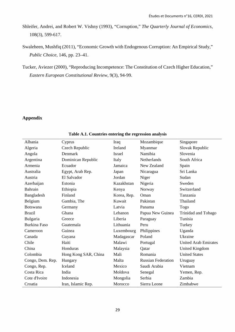
8 The full list of the countries is reported in appendix, Table A.1


20

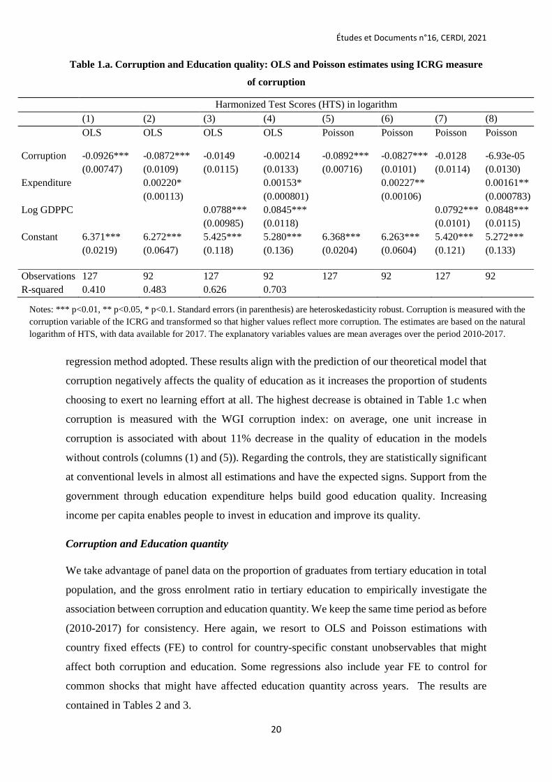
Table 1.a. Corruption and Education quality: OLS and Poisson estimates using ICRG measure

of corruption

regression method adopted. These results align with the prediction of our theoretical model that

corruption negatively affects the quality of education as it increases the proportion of students

choosing to exert no learning effort at all. The highest decrease is obtained in Table 1.c when

corruption is measured with the WGI corruption index: on average, one unit increase in

corruption is associated with about 11% decrease in the quality of education in the models

without controls (columns (1) and (5)). Regarding the controls, they are statistically significant

at conventional levels in almost all estimations and have the expected signs. Support from the

government through education expenditure helps build good education quality. Increasing

income per capita enables people to invest in education and improve its quality.

Corruption and Education quantity

We take advantage of panel data on the proportion of graduates from tertiary education in total

population, and the gross enrolment ratio in tertiary education to empirically investigate the

association between corruption and education quantity. We keep the same time period as before

(2010-2017) for consistency. Here again, we resort to OLS and Poisson estimations with

country fixed effects (FE) to control for country-specific constant unobservables that might

affect both corruption and education. Some regressions also include year FE to control for

common shocks that might have affected education quantity across years. The results are

contained in Tables 2 and 3.

Harmonized Test Scores (HTS) in logarithm (1) (2) (3) (4) (5) (6) (7) (8) OLS OLS OLS OLS Poisson Poisson Poisson Poisson

Corruption -0.0926*** -0.0872*** -0.0149 -0.00214 -0.0892*** -0.0827*** -0.0128 -6.93e-05 (0.00747) (0.0109) (0.0115) (0.0133) (0.00716) (0.0101) (0.0114) (0.0130) Expenditure 0.00220* 0.00153* 0.00227** 0.00161** (0.00113) (0.000801) (0.00106) (0.000783) Log GDPPC 0.0788*** 0.0845*** 0.0792*** 0.0848*** (0.00985) (0.0118) (0.0101) (0.0115) Constant 6.371*** 6.272*** 5.425*** 5.280*** 6.368*** 6.263*** 5.420*** 5.272*** (0.0219) (0.0647) (0.118) (0.136) (0.0204) (0.0604) (0.121) (0.133) Observations 127 92 127 92 127 92 127 92 R-squared 0.410 0.483 0.626 0.703

Notes: *** p<0.01, ** p<0.05, * p<0.1. Standard errors (in parenthesis) are heteroskedasticity robust. Corruption is measured with the corruption variable of the ICRG and transformed so that higher values reflect more corruption. The estimates are based on the natural logarithm of HTS, with data available for 2017. The explanatory variables values are mean averages over the period 2010-2017.


21

Table 1.b. Corruption and Education quality: OLS and Poisson estimates using the CPI index of TI

Table 1.c. Corruption and Education quality: OLS and Poisson estimates using the WGI Control of Corruption index

Harmonized Test Scores (HTS) in logarithm (1) (2) (3) (4) (5) (6) (7) (8) OLS OLS OLS OLS Poisson Poisson Poisson Poisson Corruption -0.113*** -0.112*** -0.0280* -0.0175 -0.110*** -0.108*** -0.0257* -0.0159 (0.00741) (0.0108) (0.0145) (0.0177) (0.00716) (0.0101) (0.0144) (0.0177) Expenditure 0.00151 0.00163** 0.00164* 0.00169** (0.00101) (0.000770) (0.000948) (0.000744) Log GDPPC 0.0681*** 0.0730*** 0.0690*** 0.0731*** (0.0103) (0.0126) (0.0104) (0.0125) Constant 6.058*** 5.998*** 5.471*** 5.370*** 6.065*** 6.000*** 5.469*** 5.372*** (0.00925) (0.0343) (0.0882) (0.105) (0.00933) (0.0329) (0.0888) (0.105) Observations 157 108 156 107 157 108 156 107 R-squared 0.476 0.567 0.610 0.705

Harmonized Test Scores (HTS) in logarithm (1) (2) (3) (4) (5) (6) (7) (8) OLS OLS OLS OLS Poisson Poisson Poisson Poisson Corruption -0.00593*** -0.00602*** -0.00173** -0.00129 -0.00580*** -0.00582*** -0.00165** -0.00124 (0.000375) (0.000542) (0.000753) (0.000899) (0.000365) (0.000511) (0.000744) (0.000890) Expenditure 0.00141 0.00154** 0.00154* 0.00160** (0.000981) (0.000768) (0.000920) (0.000742) Log GDPPC 0.0648*** 0.0694*** 0.0650*** 0.0690*** (0.0105) (0.0124) (0.0105) (0.0121) Constant 6.386*** 6.335*** 5.596*** 5.475*** 6.385*** 6.325*** 5.594*** 5.478*** (0.0199) (0.0560) (0.127) (0.149) (0.0187) (0.0523) (0.127) (0.147) Observations 152 108 151 107 152 108 151 107 R-squared 0.489 0.583 0.608 0.708

Notes: *** p<0.01, ** p<0.05, * p<0.1. Standard errors (in parenthesis) are heteroskedasticity robust. Corruption is measured with the Corruption Perception Index (CPI) of Transparency International and transformed so that higher values reflect more corruption. The estimates are based on the natural logarithm of HTS, with data available for 2017. The explanatory variables values are mean averages over the period 2010-2017

Notes: *** p<0.01, ** p<0.05, * p<0.1. Standard errors (in parenthesis) are heteroskedasticity robust. Corruption is measured with the control of corruption index of the WGI and transformed so that higher values reflect more corruption. The estimates are based on the natural logarithm of HTS, with data available for 2017. The explanatory variables values are mean averages over the period 2010-2017


22

They tend to confirm the predictions of our theoretical model as corruption is found to be

positively associated with the expected rate of success, whether measured by the proportion of

graduates (Table 2) or the gross enrolment ratio in tertiary education (Table 3). The coefficients

of corruption in Table 2 are all positive and significant at 1% or 5% levels, no matter the

measure of bribery or the regression type used. These results are confirmed in Table 3 when

using the ICRG measure of bribery in columns 1 to 4. No statistically significant link is detected

with the TI and WGI measures. Unlike GDP per capita which has the expected sign when it is

significant, government expenditure in tertiary education is found to be negatively associated

with education quantity in some of the regressions.


23

Table 2. Corruption and Education quantity: OLS and Poisson estimates using the proportion of tertiary graduates in total population as proxy for

education quantity

Proportion of graduates from tertiary education in total population (in logarithm) (1) (2) (3) (4) (5) (6) (7) (8) (9) (10) (11) (12) OLS OLS Poisson Poisson OLS OLS Poisson Poisson OLS OLS Poisson Poisson Corrup_ICRG 0.157*** 0.153*** 0.123** 0.125** (0.0514) (0.0513) (0.0537) (0.0551) Corrup_TI 0.00969** 0.0110** 0.00992** 0.0102** (0.00449) (0.00500) (0.00390) (0.00458) Corrup_WGI 0.184** 0.210** 0.236*** 0.252*** (0.0926) (0.0867) (0.0837) (0.0790) Log GDPPC 0.506 -0.0378 0.195 -0.0995 0.742** 0.357 0.429 0.383 0.342 -0.0660 0.0469 -0.191 (0.315) (0.319) (0.287) (0.270) (0.332) (0.336) (0.298) (0.274) (0.262) (0.237) (0.206) (0.177) Expenditure -0.00316* -0.00296* -0.00452** -0.00432*** -0.000525 -0.000508 -0.00171 -0.00152 -0.00362** -0.00357** -0.00518*** -0.00498*** (0.00175) (0.00150) (0.00182) (0.00166) (0.00101) (0.000926) (0.00201) (0.00179) (0.00167) (0.00146) (0.00162) (0.00152) Constant -5.412* -0.493 -7.626** -4.270 -3.436 0.194 (2.975) (2.979) (3.092) (3.080) (2.367) (2.121) Observations 354 354 343 343 282 282 262 262 419 419 400 400 R-squared 0.216 0.290 0.059 0.081 0.145 0.201 Countries 85 85 74 74 96 96 76 76 109 109 90 90 Country FE Yes Yes Yes Yes Yes Yes Yes Yes Yes Yes Yes Yes Year FE No Yes No Yes No Yes No Yes No Yes No Yes

Notes: *** p<0.01, ** p<0.05, * p<0.1. Standard errors (in parenthesis) are heteroskedasticity robust. Corrup_ICRG: WGI measure of corruption; Corrup_TI: Corruption perception index of TI; Corrup_WGI: control of corruption index of the WGI. All corruption variables are transformed so that higher values reflect more corruption. Education is measured with the proportion of graduates from tertiary education in total population. The estimates are based on yearly data over the period 2010-2017


24

Table 3. Corruption and education quantity: OLS and Poisson estimates using the gross enrolment ratio in tertiary education as proxy for education

quantity

Gross enrolment ratio in tertiary education (in logarithm) (1) (2) (3) (4) (5) (6) (7) (8) (9) (10) (11) (12) OLS OLS Poisson Poisson OLS OLS Poisson Poisson OLS OLS Poisson Poisson Corrup_ICRG 0.0666*** 0.0539** 0.0771*** 0.0735*** (0.0242) (0.0262) (0.0263) (0.0269) Corrup_TI -0.00150 -0.00140 0.00260 0.00364 (0.00303) (0.00329) (0.00210) (0.00228) Corrup_WGI -0.0992 -0.0981 -0.0233 -0.0216 (0.0958) (0.0795) (0.0788) (0.0636) Log GDPPC 0.625*** 0.189 0.468*** 0.182 0.723*** 0.407** 0.573*** 0.359** 0.630*** 0.157 0.350** 0.0328 (0.129) (0.189) (0.136) (0.163) (0.199) (0.205) (0.181) (0.168) (0.168) (0.174) (0.168) (0.175) Expenditure -0.00191*** -0.00185*** -0.00222*** -0.00211*** -0.00171** -0.00168** -0.00162** -0.00163** -0.00198*** -0.00190*** -0.00287*** -0.00270*** (0.000589) (0.000582) (0.000575) (0.000568) (0.000783) (0.000723) (0.000708) (0.000673) (0.000558) (0.000536) (0.000941) (0.000933) Constant -2.102* 1.762 -2.656 0.0655 -1.982 2.074 (1.163) (1.684) (1.709) (1.780) (1.474) (1.508) Observations 449 449 434 434 363 363 340 340 555 555 534 534 R-squared 0.365 0.443 0.230 0.264 0.201 0.269 Number of id 102 102 87 87 116 116 93 93 132 132 111 111 Country FE Yes Yes Yes Yes Yes Yes Yes Yes Yes Yes Yes Yes

Notes: *** p<0.01, ** p<0.05, * p<0.1. Standard errors (in parenthesis) are heteroskedasticity robust. Corrup_ICRG: WGI measure of corruption; Corrup_TI: Corruption Perception Index of TI; Corrup_WGI: control of corruption index of the WGI. All corruption variables are transformed so that higher values reflect more corruption. Education is measured with the gross enrolment ratio in tertiary education. The estimates are based on yearly data over the period 2010-2017


25

7. Conclusion

A simple model is developed in the context of the education sector, to highlight individuals'

heterogeneous behaviours in presence of bribery, as well as the effects of corruption on the quality

and quantity of education at the societal level.

To obtain a qualification or pass an exam, heterogeneous applicants have to pass a test, choosing

between productive effort and corrupt effort (i.e. bribery). Applicants' heterogeneity is modelled as a

difference in innate ability. There are two types of officials: honest or corrupt. Honest officials take

only learning effort into account in measuring the candidate performance, while corrupt officials care

only about the bribe size. Both effort and bribery positively contribute to the candidate's probability

of success but are costly. In case of success, the candidate obtains a degree, whose value decreases

with the proportion of corrupt officials in the economy. The key assumption of our model is that effort

and bribe are explicitly modelled as strategic substitutes.

We find that “strong” candidates rely only on effort; “medium” candidates choose positive levels of

both bribe and effort, while “weak” candidates rely only on bribery. In the presence of corruption,

such differences in behaviour result in inefficiencies in a simple way. The best candidates have a 0

probability of getting the degree when they encounter a corrupt official, while weak candidates may

still get the degree without exerting any effort.

Individual decisions also translate into aggregate effort level in the economy or aggregate expected

rate of success among applicants. Here, aggregate effort level may be interpreted as education quality,

while aggregate expected rate of success may be a proxy of education quantity. In this analysis,

aggregation is useful as it allows investigating the macro-economic effects of individual decisions

about corruption, highlighting in particular a channel (education), through which corruption may

impact growth. The results suggest that corruption may decrease education quality, as a higher

proportion of corrupt officials lowers aggregate effort level, and increases the proportion of

candidates choosing to exert no effort at all. On the other hand, corruption may increase education

quantity by increasing the chances of obtaining a degree. The empirical evidence supports these

conclusions: corruption appears to be positively correlated to both education quality (proxied with

HTS scores) and education quantity (as measured by the proportion of graduates from tertiary

education in total population; and the gross enrolment ratio in tertiary education).


26

References

Abbink, Klaus (ed.) (2006), “Laboratory Experiments on Corruption” in: S. Rose-Ackerman (eds.),

The Handbook of Corruption, Cheltenham, UK, and Northampton, US: Edward Elgar Publishers.

Ades, Alberto, and Rafael Di Tella (1999), “Rents, Competition, and Corruption,” The American

Economic Review, 89(4), 982-993.

Ades, Alberto, and Rafael Di Tella (1997), “National Champions and Corruption: Some Unpleasant

Interventionist Arithmetic,” The Economic Journal, 107 (443), 1023-1042.

Ahlin, Christian, and Pinaki Bose (2007), “Bribery, Inefficiency, and Bureaucratic delay,” Journal of

Development Economics 84 (1), 465-486.

Aidt, Toke S. (2003), “Economic Analysis of Corruption: A survey,” The Economic Journal,

113(491), 632-652.

Amir, Rabah, and Chrystie Burr (2015), “Corruption and Socially Optimal Entry,” Journal of Public

Economics, Vol. 123, pp. 30-41.

Banerjee, Abhijit V. (1997), “A Theory of Misgovernance,” The Quarterly Journal of Economics,

112(4), 1289-1332.

Bardhan, Pranab (1997), “Corruption and Development: A Review of Issues,” Journal of Economic

Literature, 35, 1320-1346.

Barro, Robert J. (2001), “Human Capital and Growth,” The American Economic Review, 91(2), 12-

17.

Beck, Paul J, and Michael W. Maher (1986), “A comparison of Bribery and Bidding in thin markets,”

Economics Letters, 20(1), 1-5.

Betts, Julian R. (1998), “The impact of educational standards on the level and distribution of

earnings,” The American Economic Review 88 (1), 266-275.

Bishop, John H. (1996), “The Impact of Curriculum-based External Examinations on school Priorities

and Student Learning,” International Journal of Education Research, 23(8), 653-752.

Bliss, Christopher, and Rafael Di Tella (1997), “Does Competition Kill Corruption?” Journal of

Political Economy, 105(5), 1001-1023.


27

Castro, Conceição, and Pedro Nunes (2013), “Does Corruption Inhibit Foreign Direct Investment?”

Política, 51(1), 61–83.

Clark, Derek J., and Christian Riis (2000), “Allocation Efficiency in a Competitive Bribery Game,”

Journal of Economic Behavior & Organization, 42(1), 109-124.

Costrell, Robert M. (1994), “A Simple Model of Educational Standards,” The American Economic

Review 84 (4), 956-971.

De Paola, Maria, and Vincenzo Scoppa (2007), “Returns to Skills, Incentives to Study and Optimal

Educational Standards,” Journal of Economics, 92(3), 229-262.

Dixit, Avinash (2002), “Incentives and Organizations in the Public Sector: An Interpretative Review,”

Journal of Human Resources 37 (4), 696-727.

Dreher, Axel, and Thomas Herzfeld (2005), “The Economic Costs of Corruption: A Survey and New

Evidence,” Working paper 0506001, Public Economics, EconWPA.

Dusek, Libor, Andreas Ortmann, and Lubomir Lizal (2005) “Understanding Corruption and

Corruptibility through experiments,” Prague Economic Papers, 14 (2), 147-162.

Drugov, Mikhail (2010), “Competition in Bureaucracy and Corruption,” Journal of Development

Economics, Vol. 92, No 2, pp. 107-114.

Eicher, Theo, Cecilia García-Peñalosa, and Tanguy van Ypersele (2009), “Education, Corruption,

and the Distribution of Income,” Journal of Economic Growth, 14, 205–231.

Fender, John (1999) “A General Equilibrium Model of Crime and punishment,” Journal of Economic

Behavior & Organization, 39 (4), 437-453.

Glaeser, Edward L., and Raven E. Saks (2006), “Corruption in America,” Journal of Public

Economics, 90, 1053-1072.

Guriev, Sergei (2004), “Red tape and corruption,” Journal of Development Economics, 73(2), 489-

504.

Hanushek, Eric A., and Dennis D., Kimko (2000), “Schooling, labor-force quality, and the growth of

nations,” The American Economic Review, 90(5), 1184-1208.

Heyneman, Stephen P. (2004), “Education and Corruption,” International Journal of Educational

Development, 24(6), 637-648.


28

Heyneman, Stephen P., Kathryn H. Anderson, and Nazym Nuraliyeva (2008), “The Cost of

Corruption in Higher Education,” Comparative Education Review, 52(1).

Huntington, Samuel P. (1968), “Political Order in Changing Societies,” New Haven and London,

Yale University.

Jain, Arvind K. (2001), “Corruption: A Review,” Journal of Economic Surveys, 15, 71-121.

Kulshreshtha, Praveen (2007), “An Efficiency and Welfare Classification of Rationing by Waiting in

the Presence of Bribery,” Journal of Development Economics, 83(2), 530-548.

Lambsdorff, Johann G. (2006), “Causes and Consequences of Corruption: What do we Know from a

Cross-section of Countries,” in: S. Rose-Ackerman (eds.), International Handbook on the

Economics of Corruption (pp. 3–51). Cheltenham, UK: Edward Elgar.

Leff, Nathaniel H. (1964), “Economic Development through Bureaucratic Corruption,” American

Behavioral Scientist, 82 (2), 337-341.

Leys, Colin (1970), “What is the problem about corruption?” in: A. Heidenheimer (eds.), Political

Corruption: Readings in Comparative Analysis. Holt Reinehart, New York.

Lien, Da-Hsiang D. (1986), “A Note on Competitive Bribery Games,” Economics Letters, 22 (4),

337-341.

Lien, Da-Hsiang D. (1990), “Corruption and Allocation Efficiency,” Journal of Development

Economics, 33(1), 153-164.

Lui, Francis T. (1985), “An Equilibrium Queuing Model of Bribery,” Journal of Political Economy,

93(4), 760-781.

Mironov, Maxim and Ekaterina Zhuravskaya (2012), “Corruption in Procurement and Shadow

Campaign Financing: Evidence from Russia”, mimeo.

Rose-Ackerman, Susan (1997), “The Political Economy of Corruption,” in: K. A. Elliott (eds.),

Corruption and the Global Economy, pp. 31-60. Washington, DC: Institute for International

Economics.

Rumyantseva, Nataliya L. (2005), “Taxonomy of Corruption in Higher Education,” Peabody Journal

of Education, 80(1), 81-92.


29

Shleifer, Andrei, and Robert W. Vishny (1993), “Corruption,” The Quarterly Journal of Economics,

108(3), 599-617.

Swaleheen, Mushfiq (2011), “Economic Growth with Endogenous Corruption: An Empirical Study,”

Public Choice, 146, pp. 23–41.

Tucker, Aviezer (2000), “Reproducing Incompetence: The Constitution of Czech Higher Education,”

Eastern European Constitutional Review, 9(3), 94-99.

Appendix

Table A.1. Countries entering the regression analysis

Albania Cyprus Iraq Mozambique Singapore Algeria Czech Republic Ireland Myanmar Slovak Republic Angola Denmark Israel Namibia Slovenia Argentina Dominican Republic Italy Netherlands South Africa Armenia Ecuador Jamaica New Zealand Spain Australia Egypt, Arab Rep. Japan Nicaragua Sri Lanka Austria El Salvador Jordan Niger Sudan Azerbaijan Estonia Kazakhstan Nigeria Sweden Bahrain Ethiopia Kenya Norway Switzerland Bangladesh Finland Korea, Rep. Oman Tanzania Belgium Gambia, The Kuwait Pakistan Thailand Botswana Germany Latvia Panama Togo Brazil Ghana Lebanon Papua New Guinea Trinidad and Tobago Bulgaria Greece Liberia Paraguay Tunisia Burkina Faso Guatemala Lithuania Peru Turkey Cameroon Guinea Luxembourg Philippines Uganda Canada Guyana Madagascar Poland Ukraine Chile Haiti Malawi Portugal United Arab Emirates China Honduras Malaysia Qatar United Kingdom Colombia Hong Kong SAR, China Mali Romania United States Congo, Dem. Rep. Hungary Malta Russian Federation Uruguay Congo, Rep. Iceland Mexico Saudi Arabia Vietnam Costa Rica India Moldova Senegal Yemen, Rep. Cote d'Ivoire Indonesia Mongolia Serbia Zambia Croatia Iran, Islamic Rep. Morocco Sierra Leone Zimbabwe


30

Table A.2. Summary statistics

Variable Obs Mean Std. Dev. Min Max Log (HTS) 1413 6.052145 0.1613995 5.720057 6.364519

Log (tertiary graduates, % pop) 778 -0.6454133 0.8439206 -4.290663 0.7786503

Log (gross enrolment ratio) 961 3.387359 0.9505207 -0.3928797 4.839314

Corruption (ICRG) 1104 3.342089 1.178687 0 5.625

Corruption (TI) 1222 57.16367 19.56328 8 92

Corruption (WGI) 1624 0.0293827 0.9991876 -2.404901 1.82574

Log (GDPPC) 1954 8.659834 1.423839 5.363194 12.1631

Expenditure 545 36.97322 14.65778 6.44574 101.8884

Notes: The statistics are based on the panel data