AALBORG UNIVERSITY ESBJERG

DEPARTMENT OF CIVIL ENGINEERING

Effect of 2nd Order Wave on Mooring Line Forces of a Floating Space Frame Structure

FLOATING SPACE FRAME STRUCTURE

by

Shravan Kantharaja

9 June 2016

iii

Title Page Title: Effect of 2nd Order Wave on Mooring Line Forces of a Float-

ing Space Frame Structure Institution: Aalborg University Esbjerg Department: Civil Engineering Supervisors: Lars Damkilde & Morten Eggert Nielsen Project period: 01/09/2015 - 09/06/2016 Author

Shravan Kantharaja Abstract

This project report contains the prediction of the mooring line forces and the prediction of the dynamic response of the floating space frame structure when subjected to a 1st order regular wave and a 2nd order regular wave. Different wave theories and the method of selecting of an appropriate wave theory is explained. A co-rotational beam formulation is implemented since the floating structures would undergo large deformations when subjected to a wave. Cylindrical beam elements are used to model all the structural elements in the project.

Relative Morison’s equation has been implemented in the project to take into account the movement of the structure when subjected to the wave forces. For validation of the wave structure interaction a simple V-shaped submerged structure is subjected to a linear regular wave and the results obtained from MATLAB and Ansys are compared. Drifting of the structure can be noticed when subjected to a 2nd order regular wave with the same wave parameters.

An anchored floating space frame structure similar to the WEPTOS Wave Energy Con-verter is modelled. This structure is subjected to a 1st order and a 2nd order wave to carry out a time domain analysis. The predicted mooring line forces and the predicted displace-ment of the structure is compared.

Total number of pages: 65

Aalborg University Esbjerg, 09 June 2016

v

Preface This thesis concludes the master degree at the Department of Civil Engineering at AAU-Aalborg University. The formulation of this thesis has been done in the 9th and the 10th semester in the period from the 1st of September 2015 to the 9th of June 2016.

The theme of the project is the effect of 2nd order wave on the Mooring Line of a floating space frame structure. This thesis focuses on the theory in addition to the numerical calculations. The numerical calculations have been carried out in Ansys Workbench and Simulation of Floaters in Action (SOFIA). The project consists of a main report and an appendix with the expansion of the formulas.

The target group for this report is civil engineers, students studying civil engineering and others interested in the considered topics. It is assumed that the reader has knowledge concerning technical subjects such as wave mechanics, wave dynamics, structural dynamics, finite element method and continuum mechanics. A copy of the report in PDF format is enclosed in the DVD. In order to use all of the enclosed material present in the DVD, Ansys Workbench and MATLAB software are required.

I want to thank my supervisors Lars Damkilde, professor at the Department of Civil Engineering at Aalborg University and Morten E. Nielsen, research assistant at Aalborg University. I appreciate your help and your guidance that I have received throughout my studies.

vi

vii

Reading guide The report is started with an introduction to the project. In the introduction the different types of ways the energy can be extracted from the ocean, followed by different type of ways the energy can be extracted from the waves is explained. This is followed by the state of art wave energy converters (WEC) that are being tested or used at present and a selection of WEC for the project.

This is followed by the description and the modelling of the waves. This chapter covers the regular waves and the irregular waves. The boundary conditions have been explained in the regular wave section as well as the method of selection of a proper wave theory based on the wave parameters. This is followed by an introduction and a detailed explanation of the linear wave theory and the second order wave theory. The irregular wave theory section covers the introduction and the explanation of the formation of an irregular wave. It also has the detailed explanation of the first order irregular wave and the second order irregular wave.

The co-rotational beam formulation chapter contains the concept of co-rotation followed by its validation. This is followed by the non-linear newmark algorithm and its validation. The next chapter is the Hydrodynamic Modelling. This chapter contains the Morison’s equation and the explanation of the different terms and the coefficients in the equation. The wave load modelling chapter contains the projection of the kinematic quantities. This is followed by the validation of the wave structure interaction and then the drift forces. The next chapter is the floating space frame structure which contains the modelling of the anchoring cable and the space frame structure similar to the WEPTOS wave energy converter. The last section of this chapter contains the dynamic response of the structure when subjected to first order regular wave and the second order regular wave.

Finally, the last chapter containe the conclusion and the explanation of all the results obtained from the project.

The literature used in thesis is shown in the bibliography, while the references in the report are symboled with e.g. [1].

ix

Nomenclature Symbols

𝜂𝜂 Surface Elevation 𝜌𝜌 Density Δ Roughness 𝜑𝜑 Velocity Potential 𝜇𝜇 Shallow Wave Parameter 𝜓𝜓 Wake Amplification Factor 𝛾𝛾 Peak Enhancement Factor 𝜅𝜅 Curvature 𝜗𝜗 Phase Angle 𝑎𝑎 Wave Amplitude As Submerged Cross-Sectional Area c Phase Velocity C Damping CA Added Mass Coefficient CD Drag Coefficient CDS Drag coefficient for the steady state flow CM Inertia Coefficient D Diameter E Young’s Modulus F Force f Frequency fp Spectral peak frequency Δ𝑓𝑓 Frequency Width g Acceleration due to Gravity HS Significant wave height h Water Depth H Wave Height I Moment of Inertia k Wave Number K Stiffness KC Keulegan-Carpenter number L Wave Length M Mass, Moment R Radius Re Reynolds Number S Wave Steepness Parameter S(f) Spectral Density T Return period; Wave period; Design wave period Tp Peak period u Horizontal Velocity ��𝑢 Horizontal Acceleration

x

um Maximum Orbital Particle Velocity Ur Ursell Parameter 𝑤𝑤 Vertical Velocity ��𝑤 Vertical Acceleration Zc Evaluation Coordinate

Abbrevations

EMEC European Marine Energy Centre LIMPET Land Installed Marine Power Energy Transmitter MWL Mean Water Level OTEC Ocean Thermal Energy Conversion OWC Oscillating Water Column SOFIA Simulation of Floaters in Action USP Underwater Substation Pod WEC Wave Energy Converter

xi

Table of Contents

1. Introduction ...................................................................................... 1 1.1 Types of Ocean Energy ......................................................................................... 1 1.2 Types of Wave Energy Converters ........................................................................ 2 1.3 State of Art Wave Energy Converters .................................................................. 4 1.4 Selection of a WEC for the project ....................................................................... 9 1.5 Aim of the project................................................................................................. 9

2. Description and Modelling of Waves .............................................. 11 2.1 Regular Waves ..................................................................................................... 11

2.1.1 Boundary Conditions ....................................................................................... 11 2.1.2 Different Wave Theories and Selection of Correct Theory ................................ 12 2.1.3 Linear Regular Wave Theory (1st Order Wave Theory) ................................... 14 2.1.4 Second Order Regular Wave Theory ................................................................ 17

2.2 Irregular Waves ................................................................................................... 21 2.2.1 JONSWAP Spectrum ....................................................................................... 22 2.2.2 First Order Irregular Waves ............................................................................. 24 2.2.3 Second Order Irregular Waves ......................................................................... 25

3. Co-rotational Beam Formulation .................................................... 30 3.1 Concept of Co-rotation ........................................................................................ 30

3.1.1 Validation of large rotation in the corotational beam formulation .................... 32 3.1.2 Validation of large deformation in corotational beam formulation .................... 34

3.2 Nonlinear Newmark Algorithm ............................................................................ 36 3.2.1 Validation ........................................................................................................ 38

3.3 Newton-Raphson Method ..................................................................................... 39 3.4 Numerical Damping ............................................................................................. 41

4. Hydrodynamic Modelling ............................................................... 42 4.1 Morison’s Equation .............................................................................................. 42 4.2 Relative Morison’s Equation ................................................................................ 43 4.3 Calculation of Hydrodynamic Coefficients............................................................ 45

4.3.1 Drag and Inertia Coefficients ........................................................................... 45 4.3.2 Added Mass Coefficient .................................................................................... 46

5. Wave Load Modelling ..................................................................... 48 5.1 Projection of the Kinematic Quantities ................................................................ 48 5.2 Extraction Points ................................................................................................. 49 5.3 Polynomial Regression of Hydrodynamic Forces .................................................. 49 5.4 Modelling of Self Weight ...................................................................................... 50 5.5 Validation of the wave structure interaction ........................................................ 51 5.6 Drift forces ........................................................................................................... 53

6. Floating Space Frame Structure ..................................................... 54

xii

6.1 Modelling of Anchoring Cable ............................................................................. 54 6.2 Modelling of the Space frame structure. .............................................................. 55 6.3 Dynamic response of the Structure ...................................................................... 55

7. Conclusion ...................................................................................... 60

Bibliography......................................................................................... 61

Appendix.............................................................................................. 63

1. Introduction An increase in the issue of global warming and a decrease in the availability of oil and other fossil fuels has led to an increasing need to find an alternative source of sustainable energy resources which will have less environmental impact. The challenge is to move from fossil based power production to a cheap, efficient and sustainable energy produc-tion. The solar, wind and bio-fuel industries are mainly leading in this aspect but research has been going on in ocean energy. Oceans cover over 70% of the Earth’s surface and represent an enormous source of renewable energy in the form of waves, tides, marine currents and thermal resources [1].

1.1 Types of Ocean Energy

Two forms of energy that are produced from the oceans are the thermal energy which uses the sun’s heat and the mechanical energy which uses the currents, tides and waves.

Ocean Thermal Energy Conversion Oceans are the world’s largest solar collectors as they cover more than 70% of the Earth’s surface. The heat from the sun causes a temperature difference between the surface of the ocean and at the ocean depth more than 1000 meters from the MWL. This temperature difference is used by the Ocean Thermal Energy Conversion or OTEC to generate elec-tricity. With only 20 degree Celsius temperature difference this form of energy can be yielded.

There are two types of OTEC technologies namely closed cycle and the open cycle. The closed cycle utilises a working fluid which has a low boiling point such as ammonia to vaporise it using the ocean’s warmth in order to turn the turbines. The vapour is con-verted back to liquid by passing it through the cold water found in the ocean depth. In the open cycle the warm sea water is actually boiled by operating it at the low pressures to convert it into steam in order to run the turbines.

OTEC plant has a very small efficiency, just a few percent. Due to this it has to work hard to produce a small amount of electricity. From the electricity produced about a third of it is used for operating the system i.e. to pump the water in and out. Since they are less efficient, they have to be constructed on a large scale which makes them an expensive investments [2] [3].

Current Energy Marine currents are the ocean water moving in a certain direction. Tides also produce currents. The mechanical energy of these currents can be converted into electricity by the use of submerged turbines which appear to be similar to a miniature version of wind turbines. The constant movement of water in the current moves the rotor blade to pro-duce electricity. There are very few of these places on Earth where sufficient energy from this method can be produced [1].

2

Tidal Energy Tides are produced due to gravitational force of the moon. Potential energy due to the difference in the water height between the low tide and the high tide is used to generate electricity.

During high tides the water comes to the shore and is trapped behind the reservoirs and during low tides this trapped water is forced through the hydro turbines. In order to capture sufficient power from the tides potential energy, the height of high tide must at least be five meters greater than the low tide. There are very few ideal locations for the construction of tidal power plant.

Wave Energy Winds produced due to differential heating of the Earth’s surface generate waves when they interact with the ocean surface, which is used for the production of electricity. When the wind energy near the surface of the water exceeds a critical value of 1m/s, one can see the water surface ripple of length 5-10cm and height 1-2cm.

Wave development is a complex process. Wind-wave interaction first transfers wind en-ergy to shorter waves. Wave-wave interaction later transfers the energy in shorter waves to energy in longer waves resulting in the growth of longer waves. Only when the compo-nent of surface wind in the direction of the wave travel exceeds the speed of wave propa-gation can the wind energy be transferred to the waves. When the intensity of the wind decreases or when the wind changes direction the waves begin to decay [4].

Wave energy represents the largest source of ocean energy. The size of the waves is de-termined by the duration to which the wind blows, its direction and the speed with which it blows. The long periodic components of these wind generated waves travel in groups called wave trains over long distances with almost no losses. This makes ocean waves a sustainable, power dense, relatively predictable and widely available source of energy [5]. The energy contained in the waves has the potential to produce up to 80,000TWh of electricity per year sufficient to meet our global energy demands five times over [6].

Wave energy is generated by the movement of the device either floating on the surface of the ocean or moored to the ocean floor. Wave energy being the largest source of ocean energy is proving to be the most commercially advanced of the ocean energy technologies with a number of companies competing for the lead. Energy production from waves is more predictable than wind, since waves come and go slowly and can be forecast 24 hours ahead. Many different techniques for converting wave energy to electric power has been studied. Some of the commonly used methods for capturing energy from waves is discussed in the following section.

1.2 Types of Wave Energy Converters

There are different types of wave energy converters. Some converters extract energy from the surface of waves. Others extract energy from the pressure fluctuations below the water surface or from the full wave. Some system are fixed in position and let waves pass by

3

them, while others follow with the waves and move with them. Figure 1.1 shows the different types of wave energy converters.

Figure 1.1: Different types of Wave Energy Converters 1. Point absorber, 2. Atten-uator, 3. Oscillating wave surge converter, 4. Oscillating water column, 5. Overtop-

ping device, 6. Submerged pressure differential [26].

The first figure is known as the point absorber which is a floating structure with its base fixed to the sea bed that absorbs energy from the waves through its movement. The point absorber converts the motion of the buoyant top relative to the base into electrical power. Electromotive force generated by electrical transmission cables and acoustic of these de-vices maybe a concern for marine organisms.

The second figure represents the surface attenuator which is also a floating device with multiple segments connected to one another and operates parallel to the direction of the wave. The attenuators rides the wave to create a flexing motion that drives the hydraulic pumps to generate electricity. They affect the environment similar to the point absorber, with an additional concern that some organism might get struck in the joints.

The third figure represents the oscillating wave surge converter. One end of this device is fixed to the sea bed while the other end is free to move. The free arm oscillates due to the movement of the water in the waves. This movement of the free arm is used to produce electricity. These devices have a minor risk of collision and also the possibility of artificial reefing near the fixed point.

The fourth figure represents the oscillating water column (OWC) which is a partially submerged structure and can be located both onshore and offshore. The device consists of an air column on top of a water column. The submerged part of the device is open to the sea. The waves causes water in the water column to rise and fall. The air gets com-pressed as the water rises and is passed through an air turbine to generate electricity. A lot of noise is produced by this process which can affect the birds and other marine organisms in the vicinity. There is also a concern of the marine organisms getting struck and entangled in the air columns.

The fifth figure represents overtopping wave energy converter. These are long structures that use the waves to increase the water level in the reservoirs with respect to the sur-rounding sea. The potential energy due to the increased water level is used to produce

4

electricity. These devices can be both onshore and offshore as floating devices. They have similar environmental problems like the previously mentioned devices.

The sixth figure is the submerged pressure differential device which is usually located near the shore and attached to the seabed. As the name indicates this device uses the pressure difference caused due to the rise and fall of sea level due to wave motion to produce electricity.

Due to a wide variety of ways through which energy can be absorbed from waves, a number of concepts and applications exists for each of them. Currently, around 254 wave energy developers are listed on the European Marine Energy Centre (EMEC) website [7]. Since there are a lot of wave energy developers, studying the WEC devices from each of them would be difficult due to time restriction. Hence, only some of the major WEC devices have been covered in the following section.

1.3 State of Art Wave Energy Converters

Some of the state of art WEC that have already been either implemented or are being tested in the lab are studied and described below.

Pelamis Wave Energy Converter (Wikipedia and EMEC website) Pelamis WEC is an offshore surface attenuator that uses the motion of the ocean surface waves to generate electricity.

Figure 1.2: Pelamis prototype machine at EMEC [26].

It operates in ocean depths of greater than 50 meter. The device is made up of sections that are connected. These sections flex and bend as the wave passes, the motion that is induced is resisted by hydraulic cylinders which pumps high pressure oil through hydrau-lic motors to generate electricity. Figure 1.2 shows the full-scale prototype of this device that was tested at EMEC in Orkney, Scotland between 2004 and 2007.

5

Pelamis device was the world’s first WEC to successfully generate electricity into a na-tional grid. The tested device in Figure 1.2 was 120 meters long, having a diameter of 3.5 meters and comprised of four tube sections.

Due to the machine’s long thin shape and low drag profile, the hydrodynamic forces are minimised, namely inertia, drag and slamming, which in large waves give rise to large loads. The device responds to the curvature of the wave rather than the wave height. Since waves can only reach a certain curvature before breaking, the range of motion through which the machine must move is limited but large motion at joints due to small waves is maintained. It should be noted that the production and utilization of the Pelamis device has been stopped.

Oyster Wave Energy Converter [6] Oyster Wave Energy Converter is an oscillating wave surge converter that captures en-ergy from near shore waves and converts it into clean sustainable energy. Figure 1.3 represents the working of this device.

Figure 1.3: Oyster Wave Energy Converter [6].

This wave power device has a mechanical buoyant hinged flap that is attached to the sea bed at depths of around 10-15 meters. The hinged flap moves forward and backward due to the nearshore waves. This movement drives two hydraulic pistons which pumps high pressure water through the flow lines to the hydroelectric power conversion plant to gen-erate electricity. By locating the device nearshore, severe storms can be avoided which occur further out to the sea. Since the power generation plant is located onshore it can be accessed anytime for inspection.

6

Wave Dragon Wave Energy Converter Wave Dragon is an overtopping device in which two wave reflectors focus waves up the ramp into an offshore reservoir. The water then returns to the ocean by the force of gravity passing through hydroelectric generators to produce electricity.

Figure 1.4: Concept of Wave Dragon [26].

The concept of wave dragon is illustrated in Figure 1.4. It uses the principle from a traditional hydropower plant in an offshore floating platform. The device is durable and heavy. Since it has only one moving i.e. the turbines compared to other WEC which have several moving parts, the chances of it getting affected due to severe weather condition is greatly reduced.

Islay LIMPET Wave Power Plant [8] Islay LIMPET (Land Installed Marine Power Energy Transmitter) Wave Power Plant works on the principle of Oscillating Water Column coupled to a well turbine or induction generator combination. This device is located on the shoreline. Figure 1.5 illustrates the working of the power plant.

Figure 1.5: Islay Limpet Wave Power Plant [8].

7

The plant has an opening at the bottom from where the waves enter and exit and in turn compress and decompress the air inside the chamber. This causes the air to flow forward and backward through a pair of contra-rotating turbines to generate electricity. It pro-vides easy maintenance as it is located onshore.

PowerBuoy Wave Energy Converter PowerBuoy is a floating power generation system that works on the concept of point absorber. Figure 1.6 illustrates the principle through which the device captures and con-verts wave energy to electricity.

Figure 1.6: PowerBuoy Wave Energy Converter [9].

A mooring keeps the device at station in the ocean. The float on the ocean surface moves along a spar in response to the ocean waves with a reduced response due to the presence of the heave plate at its base. The linear movement of the float into the spar is used by the power take-off system and is converted into a rotary motion that drives the electric generator. A number of such devices are placed together and the electricity produced by each of them is fed to USP and sent to the shore by cables. [9]

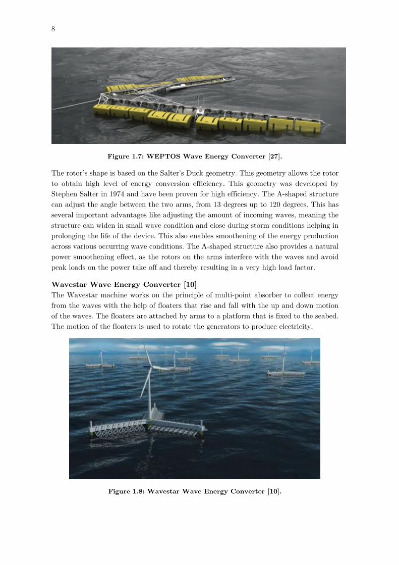
WEPTOS Wave Energy Converter [7] WEPTOS Wave Energy Converter is a floating device that uses an effective method in order to extract wave energy. The device is designed in such a way that it can regulate the amount of incoming wave energy and reduce the hydrodynamic loads during extreme wave conditions. As seen in Figure 1.7 the device is a floating A-shaped structure that absorbs the energy from the waves through a line of rotors attached to the two arms. The wave power absorbed by each of the rotors is mechanically transferred through a common axle that turns in one direction which is attached to the generator due to which an even energy is produced.

8

Figure 1.7: WEPTOS Wave Energy Converter [27].

The rotor’s shape is based on the Salter’s Duck geometry. This geometry allows the rotor to obtain high level of energy conversion efficiency. This geometry was developed by Stephen Salter in 1974 and have been proven for high efficiency. The A-shaped structure can adjust the angle between the two arms, from 13 degrees up to 120 degrees. This has several important advantages like adjusting the amount of incoming waves, meaning the structure can widen in small wave condition and close during storm conditions helping in prolonging the life of the device. This also enables smoothening of the energy production across various occurring wave conditions. The A-shaped structure also provides a natural power smoothening effect, as the rotors on the arms interfere with the waves and avoid peak loads on the power take off and thereby resulting in a very high load factor.

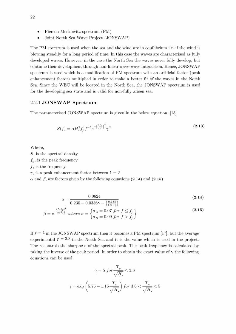
Wavestar Wave Energy Converter [10] The Wavestar machine works on the principle of multi-point absorber to collect energy from the waves with the help of floaters that rise and fall with the up and down motion of the waves. The floaters are attached by arms to a platform that is fixed to the seabed. The motion of the floaters is used to rotate the generators to produce electricity.

Figure 1.8: Wavestar Wave Energy Converter [10].

9

This device can also be installed with a wind turbine as shown in Figure 1.8 with the three arms having a number of floats to draw energy from the waves. The use of wind turbine further increases efficiency and reduces set-up cost. The device can continue pro-duction in strong winds and waves, and will automatically rise floats out of the sea when the conditions become too stormy.

1.4 Selection of a WEC for the project

A similar geometry to that of the WEPTOS WEC has been selected in this project for making further calculation which is carried out in Chapter 6. The WEPTOS WEC is based on a proven salter’s duck design, with high power to weight ratio, high load factor and effective storm survival mechanism all together [11]. The ability of the A-shaped structure to adjust angle between the two arms has helped it to maintain the amount of wave loads acting on the structure. During storm conditions, extreme loads on the struc-ture are being significantly reduced in size to such an extent that these are in the same range as those occurring during average wave conditions. This helps to avoid further strengthening the structure in order to handle the loads of extreme wave conditions. The ability of SOFIA to be able to handle such a detailed floating space frame structure is of interest, especially the importance of the effects of the first order and the second order wave theory.

1.5 Aim of the project

The aim of the report is to be able to predict the non-linear time domain response of a WEPTOS floating space frame structure subjected to a linear wave theory and a nonlinear wave theory and to determine the difference and effects of both the theories on the struc-ture and the mooring line connected to the structure.

Figure 1.9: Floating space frame structure on the water surface

In order to take into account the large motions namely rotation, translation and defor-mation which the floating space frame structure is subjected to, the co-rotational beam formulation has been implemented. The dynamic response of the structure as well as the loads that act on the structure due to the wave are predicted in time domain. The ocean

10

loads are the only environmental loads that have been considered in the project. Other environmental loads such as loads due to wind, current, ice loads etc. have not been considered. All the structural components are discretized by means of beam elements with cylindrical cross section. The prediction of the major loads and the dynamic response of the floating space frame structure is carried out in the programming language SOFIA. The results of the minor calculations have been validated against Ansys Workbench.

11

2. Description and Modelling of Waves The dominating environmental loads which the floating WEC is subjected to, are caused by the wind, waves, current and ice out of which the waves contribute to the largest amount of environmental loads. The effect of all the other loads apart from waves will not be considered in this project. This chapter deals with the regular and irregular waves, the theory and the methods used to generate these waves and the particle kinematics behind them.

2.1 Regular Waves

Waves generated due to wind develop when the wind speed is approximately 1m/s at the water surface, where the wind energy is partially transformed to wave energy due to surface shear. The below figure illustrates different parameters in a wave.

Figure 2.1: Wave Parameters

A windblown sea surface is an irregular surface, where waves continuously arise and dis-appear. Small ripples are superimposed on larger waves and the waves travel partially in different directions at different speed. Waves are classified as either long crested waves or short crested waves. Long crested waves travel in the same direction and are 3 dimensional whereas short crested waves are 2 dimensional and travel in different directions [12]. Long crested waves are considered in the rest of the report which is a good approximation in many cases.

2.1.1 Boundary Conditions

The fluid is assumed to have an irrotational flow and is assumed to be incompressible. The character of the flow of the fluid is determined by the boundary conditions. The boundary conditions are of kinematic and dynamic nature. The kinematic boundary con-dition relates to the motions of the water particles while the dynamic boundary condition relates to the forces acting on the particles. Free surface flow requires one boundary condition at the bottom and two boundary condition at the free surface. The general boundary conditions are listed below:

12

Kinematic Boundary Condition at the bottom – Since there cannot be a flow through the sea bed the vertical velocity component is zero. As the fluid is assumed to be ideal (no friction), boundary condition for the horizontal velocity at the sea bed is not included.

𝜕𝜕𝜑𝜑𝜕𝜕𝜕𝜕

= 𝑤𝑤 = 0 𝑎𝑎𝑎𝑎 𝜕𝜕 = −ℎ (2.1)

Kinematic Boundary Condition at the free surface – It specifies that the particle at the surface remains at the surface. It relates the vertical velocity of a particle at the surface to the vertical velocity of the surface.

𝜕𝜕𝜑𝜑𝜕𝜕𝜕𝜕

= 𝜕𝜕𝜂𝜂𝜕𝜕𝜕𝜕

+ 𝜕𝜕𝜂𝜂𝜕𝜕𝜕𝜕

𝜕𝜕𝜑𝜑𝜕𝜕𝜕𝜕

𝑎𝑎𝑎𝑎 𝜕𝜕 = 𝜂𝜂 (2.2)

Dynamic Boundary Condition at the free surface – It specifies that the pressure is con-stant at the surface as the pressure variations induced by the wind are not taken into account.

𝑔𝑔𝜂𝜂 + 12��𝜕𝜕𝜑𝜑

𝜕𝜕𝜕𝜕�

2+ �𝜕𝜕𝜑𝜑

𝜕𝜕𝜕𝜕�

2� + 𝜕𝜕𝜑𝜑

𝜕𝜕𝜕𝜕= 0 𝑎𝑎𝑎𝑎 𝜕𝜕 = 𝜂𝜂

(2.3)

The mathematical derivations for the boundary conditions and the governing equations can be found in Water Wave Mechanics [12].

2.1.2 Different Wave Theories and Selection of Correct Theory

A regular wave can be represented by the following theories

• Linear wave theory (Stokes 1. Order Theory) • Stokes wave theories for high waves • Stream function theory • Boussinesq higher order theory (for shallow water)

The linear wave theory is the simplest wave theory that can be applied, but it is also shown by experiments that this theory leads to unacceptable results in many cases. This is because the linear theory describes the waves as a cosine wave [13]. In reality the wave crest is shorter and steeper than the cosine wave and the wave trough is longer and less steep. To calculate the analytical solution using the linear wave theory the two boundary conditions at the surface have to be linearized (the wave amplitude ‘𝑎𝑎’ is small compared to the water depth ‘ℎ’ and therefore ‘𝐻𝐻/ℎ’ and ‘𝐻𝐻/𝐿𝐿’ have to be small) [14]. These requirements limit the linear wave theory to be represented only in very deep water. To give a more realistic description of the wave kinematics one of the other theories listed above should be used. It is also be noted that the other theories require a longer compu-tational time compared to the linear wave theory. The validity of the different theories has been covered in detail in DNV OS-J101.

Selection of Wave Theory Three parameters are used for the determination of the wave theories. The parameters are the wave height 𝐻𝐻, the wave period 𝑇𝑇 and the water depth ℎ. These parameters are

13

used to define three non-dimensional parameters that determine the validity of different theories [15].

- Wave steepness parameter 𝑆𝑆 = 2𝜋𝜋 𝐻𝐻𝑔𝑔𝑇𝑇 2 = 𝐻𝐻

𝜆𝜆𝑜𝑜

- Shallow water parameter 𝜇𝜇 = 2𝜋𝜋 ℎ𝑔𝑔𝑇𝑇 2 = ℎ

𝜆𝜆𝑜𝑜

- Ursell parameter 𝑈𝑈𝑟𝑟 = 𝐻𝐻𝑘𝑘𝑜𝑜

2ℎ3 = 14𝜋𝜋2

𝑆𝑆𝜇𝜇3

Where 𝜆𝜆𝑜𝑜 and 𝑘𝑘𝑜𝑜 are the linear deep water wavelength and the wave number correspond-ing to the wave period 𝑇𝑇 . The range of applications of the different wave theories is given in the table below.

Range of application of regular wave theories Theory Application

Depth Approximate range Linear (Airy) wave Deep and shallow water 𝑆𝑆 < 0.006; 𝑆𝑆/𝜇𝜇 < 0.03 2nd order stokes wave Deep water 𝑈𝑈𝑟𝑟 < 0.65; 𝑆𝑆 < 0.04 5th order stokes wave Deep water 𝑈𝑈𝑟𝑟 < 0.65; 𝑆𝑆 < 0. 14 Cnoidal theory Shallow water 𝑈𝑈𝑟𝑟 > 0.65; 𝜇𝜇 < 0.125

The Figure 2.2 from DNV OS-J101 can also be used to determine the wave theories to be used for different hydrodynamic load cases.

Figure 2.2: Range of validity for wave theories

14

2.1.3 Linear Regular Wave Theory (1st Order Wave Theory)

Linear wave theory also known as the small amplitude wave theory, sinusoidal wave theory or as Airy wave theory is discussed in the present section and the assumptions made are discussed. It is the simplest theory and is obtained by taking the wave height to be much smaller than both the wavelength and the water depth. For a regular linear wave the height of the crest is equal to the height of the trough i.e. the wave amplitude is half the wave height. The theory assumes that the fluid has a uniform mean depth, and that the fluid flow is inviscid, incompressible and ir-rotational. This theory is only valid for non-breaking waves with small amplitude.

This theory gives the linearized description of the propagation of gravity waves on the surface of a homogenous fluid layer. By assuming 𝐻𝐻𝐿𝐿 ≪ 1, i.e. small amplitude, the bound-ary conditions can be linearized and 𝜂𝜂 is eliminated. This means that the surface condition is valid for 𝜕𝜕 = 0 instead of 𝜕𝜕 = 𝜂𝜂. The surface elevation of this theory is denoted by

𝜂𝜂(1) = 𝐻𝐻2

cos (𝜔𝜔𝜕𝜕 − 𝑘𝑘𝜕𝜕) (2.4)

The surface elevation obtained by the use of (2.4) with ℎ = 30𝑚𝑚,𝑇𝑇 = 11𝑎𝑎 and 𝐻𝐻 = 13𝑚𝑚 is shown in the Figure 2.3.

Figure 2.3: Surface Profile for a 1st order regular wave

The velocity potential for the 1st order wave theory is

15

𝜑𝜑(1) = −𝑎𝑎𝑔𝑔𝜔𝜔

cosh (𝑘𝑘(𝜕𝜕 + ℎ))cosh (𝑘𝑘ℎ)

sin (𝜔𝜔𝜕𝜕 − 𝑘𝑘𝜕𝜕) (2.5)

Where 𝑘𝑘 and 𝑎𝑎 are the wave number and wave amplitude respectively. Detailed descrip-tion and derivation of the velocity potential is given in [12]. The velocity field can be found out by differentiating the velocity potential from (2.5) and the acceleration fields can be found out by differentiating the velocities with respect to time as shown below.

𝑢𝑢(1) = 𝜕𝜕𝜑𝜑𝜕𝜕𝜕𝜕

(2.6)

𝑤𝑤(1) = 𝜕𝜕𝜑𝜑𝜕𝜕𝜕𝜕

(2.7)

��𝑢(1) = 𝜕𝜕𝑢𝑢𝜕𝜕𝜕𝜕

(2.8) ��𝑤(1) = 𝜕𝜕𝑤𝑤𝜕𝜕𝜕𝜕

(2.9)

Theoretically the expressions in (2.6) to (2.9) are only valid for 𝐻𝐻𝐿𝐿 ≪ 1, i.e. in the inter-val −ℎ < 𝜕𝜕 ≅ 0. However, it is quite common to use the expressions for the negative and the positive values of 𝜂𝜂, i.e. also for 𝜕𝜕 = 𝜂𝜂. But this gives a crude approximation as the theory is not valid near the surface. Hence wheeler stretching of the velocity profiles and the acceleration profiles is done. In wheeler stretching the profiles are stretched and com-pressed as shown in Figure 2.4. This is done so that the evaluation coordinate 𝜕𝜕𝑐𝑐 is never positive. The evaluation coordinate is given by 𝜕𝜕𝑐𝑐 = ℎ(𝑧𝑧−𝜂𝜂)

ℎ+𝜂𝜂 where 𝜂𝜂 is the instantaneous water surface elevation.

Figure 2.4: Wheeler Stretching Modification [16]

The horizontal velocity and the horizontal acceleration as well as the vertical velocity and vertical acceleration at a depth of -11m below the mean water level of the regular wave shown in Figure 2.3 is calculated and shown in Figure 2.5. As expected the horizontal acceleration is zero at the crest and trough of the wave whereas the horizontal velocity is the highest at the crest of the wave and lowest at the trough of the wave. Similarly the vertical acceleration is lowest at the crest at the crest of the wave and highest at the trough of the wave whereas the vertical velocity remains zero at both these places. The

16

first order regular wave profile as well as the velocities and accelerations have been com-pared to WAVELAB [17] and validated.

Figure 2.5: Velocity and Acceleration at a depth of -11m below MWL

Validation of the first order regular wave theory In this section the first order regular wave theory programmed in MATLAB has been validated against the first order theory in WAVELAB [17].

Figure 2.6: Comparison of 1st order elevation from WAVELAB and MATLAB

-8

-6

-4

-2

0

2

4

6

8

0 5 10 15 20 25 30 35

Ele

vatio

n [m

]

Time [sec]

WAVELAB

MATLAB

17

Figure 2.6 shows the elevation of the 1st order regular wave having a wave height, water depth and time period of 13m, 30m and 11sec respectively. The surface elevation obtained from WAVELAB lies exactly on the surface elevation obtained from MATLAB. For val-idating the first order wave kinematics, the horizontal and vertical velocities and acceler-ations were chosen at random in MATLAB and seen at the same point in WAVELAB and the results were exactly the same. Hence, validating the surface elevation and the wave kinematics of the first order regular wave theory.

2.1.4 Second Order Regular Wave Theory

In practice many waves have a steepness 𝐻𝐻𝐿𝐿 so large that the calculations done by the linear wave theory does not describe the real wave properly and are too inaccurate. In order to describe the real waves better than the 1st order theory allows, we must discard fewer terms in the linearized boundary conditions. Furthermore, we need to introduce an extra boundary condition, if we want to fulfil the boundary conditions at 𝜕𝜕 = 𝜂𝜂 instead of at 𝜕𝜕 = 0. In the real wave it is seen that both the wave crest (𝜂𝜂 > 0) and the wave trough (𝜂𝜂 < 0) are lifted compared to the cosine wave. In order to better describe the regular waves Stokes higher order wave theories are used in which the surface elevation is given by

𝜂𝜂 = 𝜂𝜂(1) + 𝜂𝜂(2) + ⋯ + 𝜂𝜂(𝑖𝑖) (2.10) Where 𝑖𝑖 represents the order of the theory. Therefore the 2nd order Stokes regular wave theory contains an extra component in addition to the 1st order term.

Figure 2.7: 1st order and 2nd order regular wave

18

The expression for the 2nd order surface elevation component is given below

𝜂𝜂(2) = 𝐻𝐻2

𝐻𝐻𝐿𝐿

𝜋𝜋4

(3 coth3 𝑘𝑘ℎ − coth 𝑘𝑘ℎ) cos 2(𝜔𝜔𝜕𝜕 − 𝑘𝑘𝜕𝜕) (2.11)

The above expression when added to the 1st order surface profile given in (2.4), gives the surface profile for the 2nd order. The figure below shows the 2nd order regular wave and the 1st order regular wave. The Figure 2.7 was calculated for a water depth of 30m, wave height 13m and a wave period of 11sec. It can be seen in the figure that the 2nd order wave has a shorter and steeper wave crest than the 1st order wave, also the trough for the 2nd order regular wave is longer and less steep which better describes the real wave. It can also be seen that the 2nd order component is oscillating twice as fast as the 1st order term.

Figure 2.8: Location of wave parameters

The selection of the wave based on the parameters used for Figure 2.7 and Figure 2.11 are shown in Figure 2.8. A different wave parameter is selected in the validation section as this lies deeper in the 2nd order wave region.

Similar to the surface elevation, the velocity potential of the 2nd order wave is the sum-mation of the velocity potential of the 1st order wave and the velocity potential of the 2nd order component. The velocity potential of the 2nd order wave is given below

19

𝜑𝜑 = 𝜑𝜑(1) + 332

𝑐𝑐𝑘𝑘𝐻𝐻2cosh (2𝑘𝑘(𝜕𝜕 + ℎ))sinh4(𝑘𝑘ℎ)

sin�2(𝜔𝜔𝜕𝜕 − 𝑘𝑘𝜕𝜕)� − 18𝑔𝑔𝐻𝐻2𝜕𝜕

𝑐𝑐ℎ (2.12)

To obtain the velocities and accelerations from the velocity potential (2.6) to (2.9) are used.

Figure 2.9: Velocity at -11m below MWL

Figure 2.9 compares the horizontal and vertical velocities obtained from the 1st order theory and the 2nd order theory a well as the contribution of the 2nd order component. In the figure it is noticed that the 2nd order wave theory as expected gives a higher velocity when compared to the 1st order wave theory.

20

Figure 2.10: Acceleration at -11m below MWL

Figure 2.10 compares the horizontal and vertical accelerations obtained from the 1st order theory and the 2nd order theory a well as the contribution of the 2nd order component. Kinematics obtained from a 2nd and above order wave theory can be used to validate the kinematics of the 2nd order wave theory which has been done in this case and is validated with the kinematics of the 5th order wave theory obtained in WAVELAB.

Validation of the second order regular wave theory In this section the second order regular wave theory programmed in MATLAB has been validated against the fifth order regular wave theory in WAVELAB [17].

21

Figure 2.11: Comparison of elevation from 5th order WAVELAB and 2nd order MATLAB

Since the second order wave theory hasn’t been programmed in WAVELAB, the fifth order wave theory is used for validation. Appendix A1 contains the script for the 2nd order regular wave theory. The use of a higher order wave theory for validation shouldn’t be a problem as when a lower order wave theory is valid, the higher order wave theory should also give the same results but would require more computational time. Figure 2.11 shows the surface elevation of the 5th order regular wave obtained from WAVELAB and the 2nd order regular wave obtained from MATLAB having a wave height, water depth and time period of 7m, 30m and 11sec respectively. The surface elevation obtained from WAVELAB lies exactly on the surface elevation obtained from MATLAB. For validating the wave kinematics, the horizontal and vertical velocities and accelerations were chosen at random in MATLAB and seen at the same point in WAVELAB and the results were exactly the same. Hence, validating both the surface elevation and the wave kinematics of the second order regular wave theory. The use of a higher order wave theory shows a more realistic wave as well as the drift forces are taken into account by use of a higher order wave theory compared to the first order theory where the drift is not taken into account.

2.2 Irregular Waves

Modelling and realistic representation of wind generated waves and swells require the introduction of irregular waves. A real sea state is best described by the irregular wave, since the waves in the ocean are irregular in shape, length, height and phase. If the surface elevation of the irregular wave is available over a time series then the frequency domain analysis can be used to study the irregular waves. But for the project since no wave data is available, irregular waves are generated arbitrarily. Irregular waves are modelled by superposition of 𝑁𝑁 number of regular waves. Two theories which are mainly used for generation of irregular waves are

-4

-3

-2

-1

0

1

2

3

4

5

0 5 10 15 20 25 30 35Ele

vatio

n []m

Time [sec]

5th order WAVELAB

2nd order MATLAB

22

• Pierson-Moskowitz spectrum (PM) • Joint North Sea Wave Project (JONSWAP)

The PM spectrum is used when the sea and the wind are in equilibrium i.e. if the wind is blowing steadily for a long period of time. In this case the waves are characterised as fully developed waves. However, in the case the North Sea the waves never fully develop, but continue their development through non-linear wave-wave interaction. Hence, JONSWAP spectrum is used which is a modification of PM spectrum with an artificial factor (peak enhancement factor) multiplied in order to make a better fit of the waves in the North Sea. Since the WEC will be located in the North Sea, the JONSWAP spectrum is used for the developing sea state and is valid for non-fully arisen sea.

2.2.1 JONSWAP Spectrum

The parameterised JONSWAP spectrum is given in the below equation. [13]

Where, 𝑆𝑆, is the spectral density 𝑓𝑓𝑝𝑝, is the peak frequency 𝑓𝑓 , is the frequency 𝛾𝛾, is a peak enhancement factor between 𝛼𝛼 and 𝛽𝛽, are factors given by the following equations (2.14) and (2.15)

𝛼𝛼 = 0.06240.230 + 0.0336𝛾𝛾 − �0.185

1.9+𝛾𝛾� (2.14)

𝛽𝛽 = 𝑒𝑒−�𝑓𝑓−𝑓𝑓𝑝𝑝�2

2𝜎𝜎2𝑓𝑓𝑝𝑝2 𝑤𝑤ℎ𝑒𝑒𝑒𝑒𝑒𝑒 𝜎𝜎 = �𝜎𝜎𝐴𝐴 = 0.07 𝑓𝑓𝑓𝑓𝑒𝑒 𝑓𝑓 ≤ 𝑓𝑓𝑝𝑝𝜎𝜎𝐵𝐵 = 0.09 𝑓𝑓𝑓𝑓𝑒𝑒 𝑓𝑓 > 𝑓𝑓𝑝𝑝

� (2.15)

If in the JONSWAP spectrum then it becomes a PM spectrum [17], but the average experimental in the North Sea and it is the value which is used in the project. The 𝛾𝛾 controls the sharpness of the spectral peak. The peak frequency is calculated by taking the inverse of the peak period. In order to obtain the exact value of 𝛾𝛾 the following equations can be used

𝛾𝛾 = 5 𝑓𝑓𝑓𝑓𝑒𝑒𝑇𝑇𝑝𝑝

�𝐻𝐻𝑠𝑠≤ 3.6

𝛾𝛾 = exp�5.75 − 1.15𝑇𝑇𝑝𝑝

�𝐻𝐻𝑠𝑠�𝑓𝑓𝑓𝑓𝑒𝑒 3.6 <

𝑇𝑇𝑝𝑝

�𝐻𝐻𝑠𝑠< 5

𝑆𝑆(𝑓𝑓) = 𝛼𝛼𝐻𝐻𝑠𝑠2𝑓𝑓𝑝𝑝

4𝑓𝑓−5𝑒𝑒−54�𝑓𝑓𝑝𝑝

𝑓𝑓 �4

𝛾𝛾𝛽𝛽 (2.13)

23

𝛾𝛾 = 1 𝑓𝑓𝑓𝑓𝑒𝑒 5 ≤𝑇𝑇𝑝𝑝

�𝐻𝐻𝑠𝑠

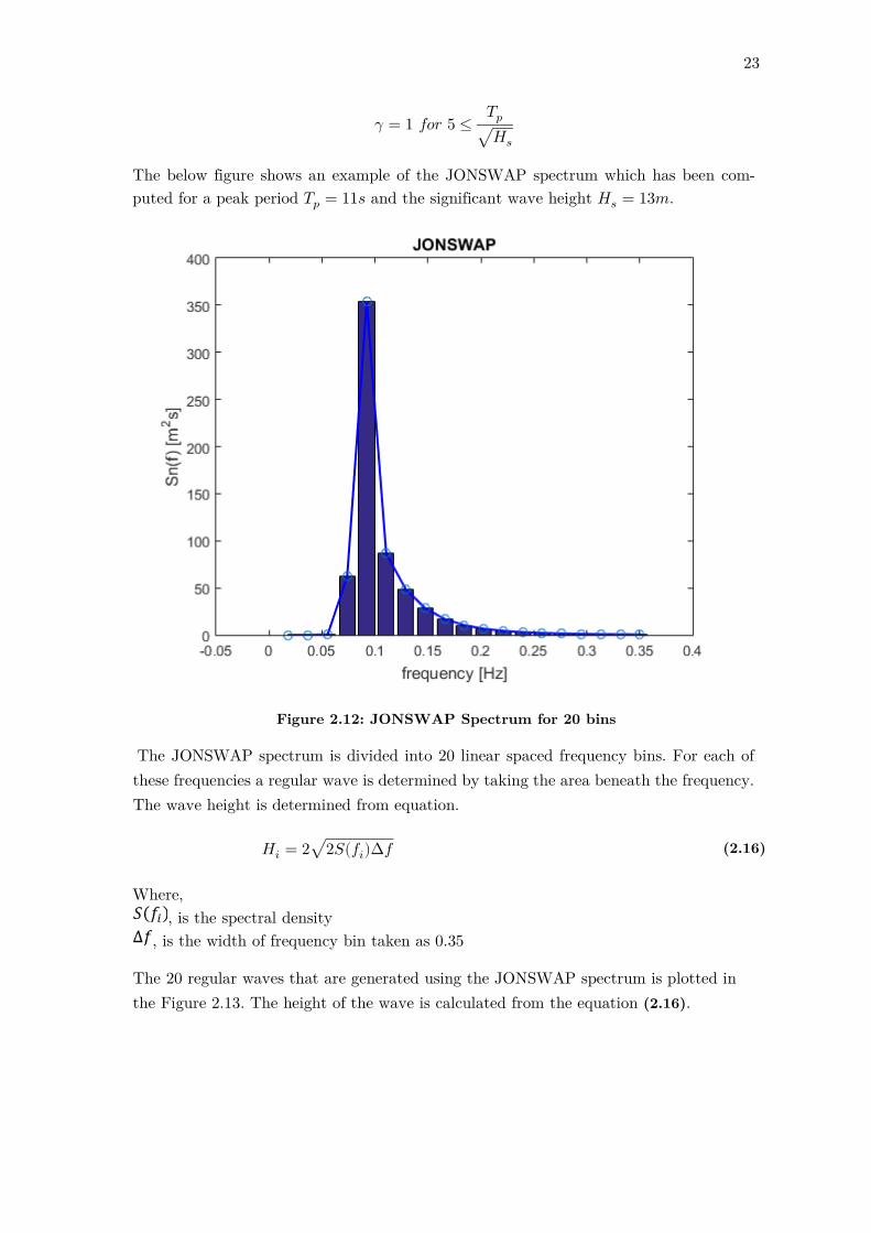
The below figure shows an example of the JONSWAP spectrum which has been com-puted for a peak period 𝑇𝑇𝑝𝑝 = 11𝑎𝑎 and the significant wave height 𝐻𝐻𝑠𝑠 = 13𝑚𝑚.

Figure 2.12: JONSWAP Spectrum for 20 bins

The JONSWAP spectrum is divided into 20 linear spaced frequency bins. For each of these frequencies a regular wave is determined by taking the area beneath the frequency. The wave height is determined from equation.

𝐻𝐻𝑖𝑖 = 2�2𝑆𝑆(𝑓𝑓𝑖𝑖)∆𝑓𝑓

(2.16)

Where, , is the spectral density

, is the width of frequency bin taken as 0.35

The 20 regular waves that are generated using the JONSWAP spectrum is plotted in the Figure 2.13. The height of the wave is calculated from the equation (2.16).

24

Figure 2.13: 20 Regular waves from JONSWAP Spectrum

2.2.2 First Order Irregular Waves

The common approach to simulate a random wave field is to superimpose all the regular waves obtained in the JONSWAP spectrum shown in Figure 2.13. This superimposing or the summation of the regular waves will produce an irregular wave. According to the linear wave theory or the first order theory, the surface elevation can be expressed as follows

𝜂𝜂(1) = �𝑎𝑎𝑛𝑛cos (𝜔𝜔𝑛𝑛𝜕𝜕 − 𝑘𝑘𝜕𝜕 − 𝜗𝜗𝑛𝑛)𝑁𝑁

𝑛𝑛=1

(2.17)

Where, 𝑎𝑎𝑛𝑛, is the wave amplitude 𝜔𝜔𝑛𝑛, is the wave frequency 𝜗𝜗𝑛𝑛, is the phase angle

The wave profile for the first order irregular wave is written as the summation of cosine terms which is given in the equation (2.17). The regular waves will have different phase angles, which is obtained randomly from uniformly distributing the phase angles 𝜗𝜗𝑛𝑛 be-tween 0 and 2𝜋𝜋. The velocity potential of the First order irregular wave that corresponds to the surface elevation given in equation (2.17) reads

𝜑𝜑(1) = �𝑏𝑏𝑛𝑛cosh�𝑘𝑘𝑛𝑛(𝜕𝜕 + ℎ)�

cosh(𝑘𝑘𝑛𝑛ℎ)sin(𝜔𝜔𝑛𝑛𝜕𝜕 − 𝑘𝑘𝑛𝑛𝜕𝜕 − 𝜗𝜗𝑛𝑛)

𝑁𝑁

𝑛𝑛=1

(2.18)

25

Where 𝑏𝑏𝑚𝑚 is the amplitude coefficient given by 𝑏𝑏𝑛𝑛 = 𝑎𝑎𝑛𝑛𝑔𝑔𝜔𝜔𝑛𝑛

. In the reference system used in these expressions, 𝜕𝜕 is positive in the propagation direction of the waves. The vertical coordinate 𝜕𝜕 is positive upwards and is zero at mean sea level. From the above velocity potential the expressions for the first order horizontal and vertical velocities and acceler-ations can be obtained by differentiating as shown in equations (2.6) to (2.9). The surface elevation obtained for the first order irregular wave is shown in Figure 2.14.

Figure 2.14: Surface Elevation of 1st Order Irregular Wave

2.2.3 Second Order Irregular Waves

The first order irregular wave doesn’t show the actual wave as the interactions between the wave components are neglected in it. The second order irregular wave model predicts more realistic crest height distribution [18], which means higher individual wave crests and consequently more realistic and higher viscous contributions above the still water level, especially for large sea states. The second order irregular wave is generated by adding the second order correction to the first order wave profile. The second order accu-rate sea surface elevation is a perturbation expansion of the first order formulation and is given as

𝜂𝜂(2)(𝑡𝑡) = 𝜂𝜂(1) + Δ𝜂𝜂(2) = 𝜂𝜂(1) + ∆𝜂𝜂(2+) + ∆𝜂𝜂(2−) (2.19)

26

The ∆𝜂𝜂(2+) and Δ𝜂𝜂(2−) are the difference and sum frequency corrections also known as the sub and super harmonics which is given as [19]

Δ𝜂𝜂(2)(𝑡𝑡) = � �[𝑎𝑎𝑚𝑚𝑎𝑎𝑛𝑛{𝐵𝐵𝑚𝑚𝑛𝑛+ cos�𝜓𝜓𝑚𝑚 + 𝜓𝜓𝑛𝑛� + 𝐵𝐵𝑚𝑚𝑛𝑛

− cos�𝜓𝜓𝑚𝑚 − 𝜓𝜓𝑛𝑛�}] 𝑁𝑁

𝑛𝑛=1

𝑁𝑁

𝑚𝑚=1

(2.20)

The expressions for the transfer functions of the 2nd order amplitude, 𝐵𝐵𝑚𝑚𝑛𝑛+ and 𝐵𝐵𝑚𝑚𝑛𝑛

− are lengthy and are therefore given in the appendix section.

The positive interaction term in the equation (2.20) produce the sharpening of the crests and flattening of the troughs which is associated with the second-order stokes wave. The negative interaction term given in the equation (2.20), gives the set down of the water level under wave groups.

Figure 2.15: Surface Profile of First and Second order Components

Therefore, the sum of first order irregular wave surface elevation given in equation (2.17) and the second order surface correction given in equation (2.20) gives the second order accurate sea surface elevation. The Surface profiles of the first order irregular wave and the second order surface correction given in equation (2.19) is shown in Figure 2.15.

27

Figure 2.16: 2nd Order and 1st Order Irregular wave

The summation of the 1st order irregular wave with the 2nd order component give the second order irregular wave profile. Figure 2.16 shows surface elevation of the first order irregular wave and the second order irregular wave and also the second order surface correction. This irregular wave is produced by the 20 regular waves shown in the Figure 2.13. Due to the difference in the wave profile the kinematics obtained will also be differ-ent. The second order irregular wave will have a higher velocity and acceleration when compared to the first order irregular wave as it takes wave to wave interaction into account. As expected the 2nd order irregular wave produces higher crest and lower trough when compared to the 1st order irregular wave which is also the same for regular wave which is shown in Figure 2.7.

Similar to the surface elevation of the second order wave, the wave parameters can be expressed as a summation of the 1st and 2nd order terms of the velocity potential and its derivatives.

𝜑𝜑(2) = 𝜑𝜑(1) + ∆𝜑𝜑(2)

(2.21)

The second order difference and sum velocity potential that corresponds to the surface elevation perturbations from equation (2.21) is given below

∆𝜑𝜑(2)(𝜕𝜕, 𝜕𝜕) = 14

� ��𝑏𝑏𝑚𝑚𝑏𝑏𝑛𝑛cosh (𝑘𝑘𝑚𝑚𝑛𝑛

± (𝜕𝜕 + ℎ))cosh (𝑘𝑘𝑚𝑚𝑛𝑛

± ℎ)𝐷𝐷𝑚𝑚𝑛𝑛

±

(𝜔𝜔𝑚𝑚 ± 𝜔𝜔𝑛𝑛)sin(𝜓𝜓𝑚𝑚 ± 𝜓𝜓𝑛𝑛)�

𝑁𝑁

𝑛𝑛=1

𝑁𝑁

𝑚𝑚=1

(2.22)

28

In the similar way as for the first order kinematics, second order perturbation contribu-tions can be obtained by differentiating the above velocity potential. The addition of equations (2.18) and (2.22) gives the velocity potential of the second order irregular wave. The velocity potential is differentiated with respect to ′𝜕𝜕′and ′𝜕𝜕′ to obtain the horizontal velocity ′𝑢𝑢′ and the vertical velocity ′𝑤𝑤′ which is shown in the appendix. The horizontal and the vertical velocities obtained at -11m below the Mean Water Level (MWL) is shown in Figure 2.17.

Figure 2.17: Horizontal and Vertical Velocities at a depth of -11 meters below MWL

Figure 2.17 compares the velocities obtained for the 1st order irregular wave, 2nd order irregular wave contribution and the 2nd order irregular wave which is the sum of the velocities of the 1st order irregular wave and the 2nd order contribution at the same depth.

29

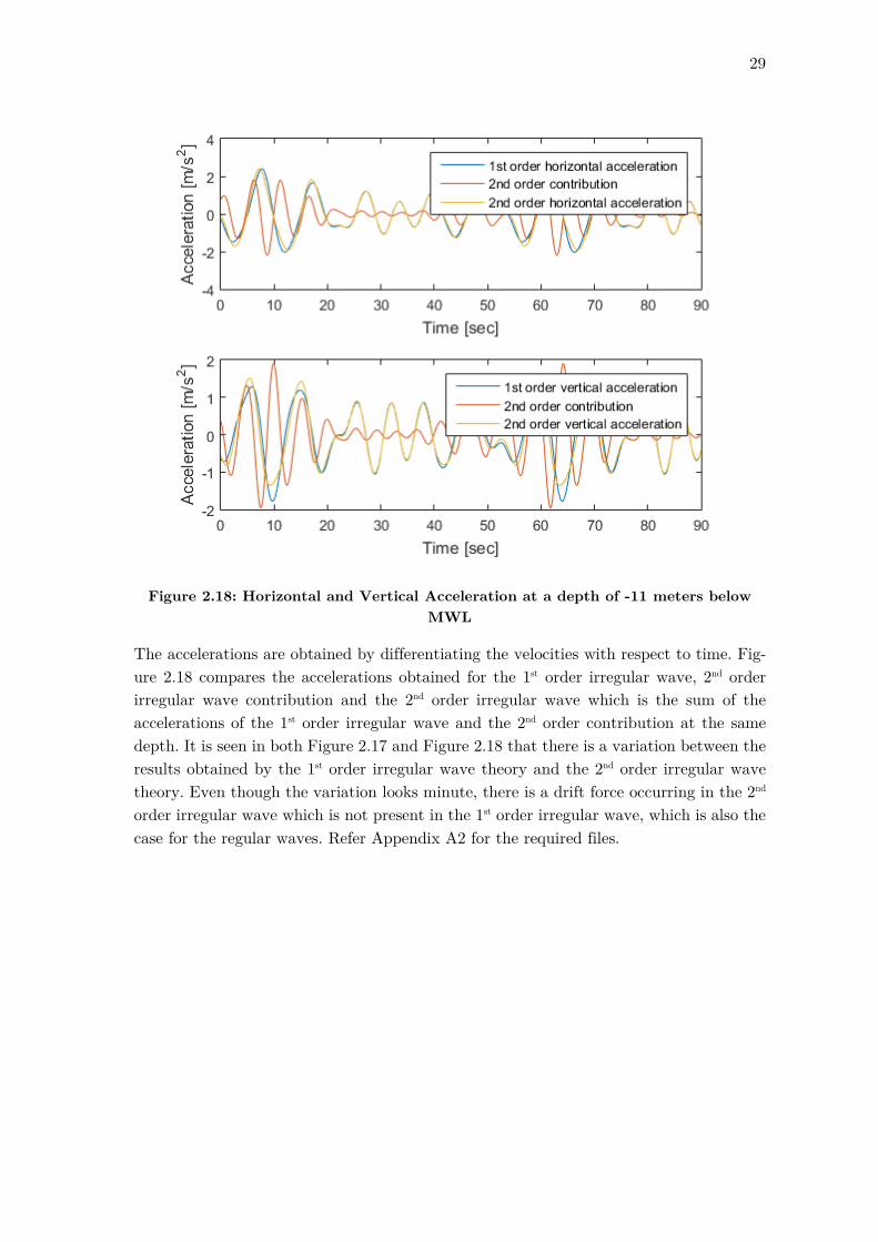
Figure 2.18: Horizontal and Vertical Acceleration at a depth of -11 meters below MWL

The accelerations are obtained by differentiating the velocities with respect to time. Fig-ure 2.18 compares the accelerations obtained for the 1st order irregular wave, 2nd order irregular wave contribution and the 2nd order irregular wave which is the sum of the accelerations of the 1st order irregular wave and the 2nd order contribution at the same depth. It is seen in both Figure 2.17 and Figure 2.18 that there is a variation between the results obtained by the 1st order irregular wave theory and the 2nd order irregular wave theory. Even though the variation looks minute, there is a drift force occurring in the 2nd order irregular wave which is not present in the 1st order irregular wave, which is also the case for the regular waves. Refer Appendix A2 for the required files.

30

3. Co-rotational Beam Formulation Since the WEC will be subjected to large displacements and rotations due to the action of the waves, it cannot be neglected that loads may change their orientation according to the displacements and the supports may change during the loading. Therefore, an efficient beam element formulation has to be developed. In this chapter an introduction to a simple two-dimensional co-rotational beam formulation is done. The main ideas of co-rotational approach can be summarised by defining an element reference frame that translates and rotates with the element’s overall rigid body motion, but does not deform with the ele-ment. By calculation of the nodal variables with respect to this reference frame, the ele-ment’s overall rigid-body motion is thus excluded in the computation of the local internal force vector and the element tangent stiffness matrix, resulting in an element-independent formulation. By the geometric nonlinearity which are induced by the large element rigid-body motion which is incorporated in the transformation matrix relating the local and global internal force vector and tangent stiffness matrix [20].

The structural nonlinearities that can be identified are the geometric nonlinearities, ma-terial nonlinearities and boundary nonlinearities. The geometric nonlinearities are signif-icant in the WEC and are included in the project. The material nonlinearities have not been included in the project. The structure supports and the insistence of the degrees of freedom which are part of the boundary nonlinearities are included as the modelled forces and are set as a function of the updated node coordinates and thus as a function of the displacements.

3.1 Concept of Co-rotation

A floating structure will undergo large displacement and rotation unless it is somehow constrained to avoid it. Large rigid body motions are allowed in a co-rotational beam theory where as it is not allowed in the regular beam theory which is a problem. The co-rotational concept in terms of beam elements is valid as long as the element strains are small and all beam elements are assumed to remain linear elastic. Unlike a regular beam theory where deformations and rotations are defined with reference to the global coordi-nate system, the co-rotational beam theory uses the element based local coordinate sys-tem. When a load is applied on a frame structure, the entire frame deforms from its original configuration. During this process each individual beam element potentially does three things; it rotates, translates and deforms. The global displacements of the end nodes of the beam element has the information about how the beam element has rotated, trans-lated and deformed from its initial position. If the rotation and translation which are rigid body motions are removed from the motion of the beam all that will remain are the strain that are causing deformations of the beam element. These strain causing local defor-mations are related to the forces that are induced in the beam element.

A co-rotational formulation thus tries to separate the rigid body motions from the strain producing deformations at the local element level. To accomplish this, a local element

31

reference frame (or coordinate system) is attached to each element. This coordinate sys-tem rotates and translates with the beam element. With respect to this local co-rotating coordinate frame the rigid body rotations and translations are zero and only local strain producing deformations remain [21]. As shown in the Figure 3.1 the x-axis is directed along the element and the y-axis is perpendicular to it.

Figure 3.1: Initial and current position of co-rotating beam elements

The figure shows a beam element in its initial and current configuration. The beam ele-ment has translated and rotated from its initial configuration to the current configuration. The beam also has local flexural deformations. In the above figure 𝛽𝛽0 is the initial angle and 𝛽𝛽 is the current angle of the beam. The initial configuration of the global nodal coordinate axis for node 1 is (𝑋𝑋1, 𝑌𝑌1) and for node 2 is (𝑋𝑋2, 𝑌𝑌2). Then the original length of the beam is

𝐿𝐿𝑜𝑜 = �(𝑋𝑋2 − 𝑋𝑋1)2 + (𝑌𝑌2 − 𝑌𝑌1)2 (3.1)

The beam element is moved from the initial configuration to the current configuration having the global nodal coordinate as (𝑋𝑋1 + 𝑢𝑢1, 𝑌𝑌1 + 𝑤𝑤1) for node 1 and (𝑋𝑋2 + 𝑢𝑢2, 𝑌𝑌2 +𝑤𝑤2) for node 2, where 𝑢𝑢1 is the global nodal displacement of node 1 in x-direction and 𝑤𝑤1 is the global nodal displacement of node 1 in y-direction. Then the current length of the beam is given as

𝐿𝐿 = ��(𝑋𝑋2 + 𝑢𝑢2) − (𝑋𝑋1 + 𝑢𝑢1)�2 + �(𝑌𝑌2 + 𝑤𝑤2) − (𝑌𝑌1 + 𝑤𝑤1)�

2 (3.2)

32

The initial and the current angle of rotation are 𝛽𝛽𝑜𝑜 and 𝛽𝛽 respectively which are defined by the global variables and are used in the calculation of 𝜃𝜃1𝑙𝑙 and 𝜃𝜃2𝑙𝑙 which are the local nodal rotations. These local nodal rotations allow the two-dimensional beam element to have arbitrarily large rotations and are used in the calculation of the local end mo-ments 𝑀𝑀1 and 𝑀𝑀2 of the beam element.

For a more detailed description of the concept and theory of the co-rotational beam formulation reference is made to the paper presented by Louie L. Yaw [21]. The validation of the co-rotational beam elements is shown below.

3.1.1 Validation of large rotation in the corotational beam formulation

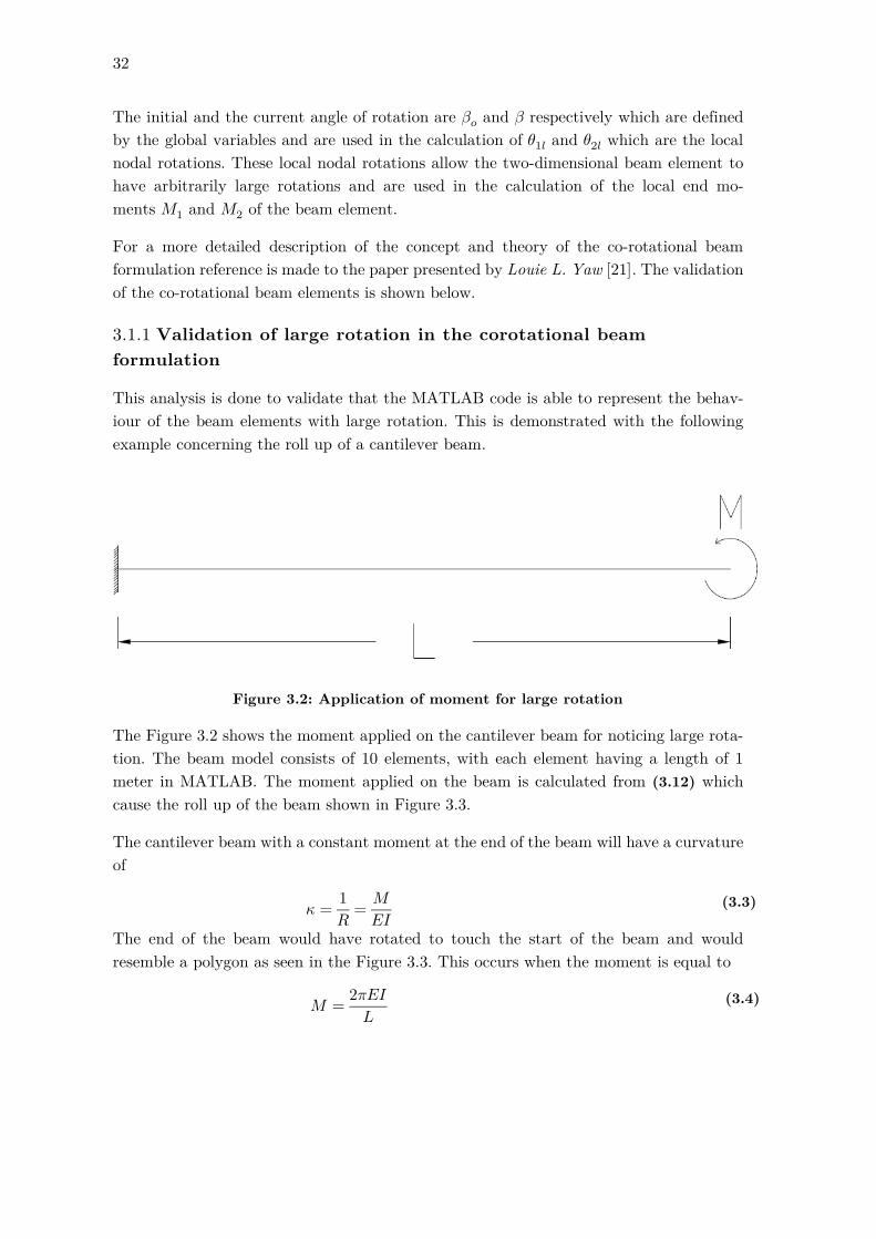
This analysis is done to validate that the MATLAB code is able to represent the behav-iour of the beam elements with large rotation. This is demonstrated with the following example concerning the roll up of a cantilever beam.

Figure 3.2: Application of moment for large rotation

The Figure 3.2 shows the moment applied on the cantilever beam for noticing large rota-tion. The beam model consists of 10 elements, with each element having a length of 1 meter in MATLAB. The moment applied on the beam is calculated from (3.12) which cause the roll up of the beam shown in Figure 3.3.

The cantilever beam with a constant moment at the end of the beam will have a curvature of

𝜅𝜅 = 1𝑅𝑅

= 𝑀𝑀𝐸𝐸𝐸𝐸

(3.3)

The end of the beam would have rotated to touch the start of the beam and would resemble a polygon as seen in the Figure 3.3. This occurs when the moment is equal to

𝑀𝑀 = 2𝜋𝜋𝐸𝐸𝐸𝐸𝐿𝐿

(3.4)

33

Figure 3.3: Roll up of the cantilever beam in MATLAB

Only beam theories that can handle large rotations will be able to model this phenomena. The same result is achieve every time since the applied moment is dependent on the beam dimension and properties. Since the example requires a static solving method, the moment is incrementally increased over a sufficient amount of time.

34

Figure 3.4: Moment vs Displacement plot

The above figure shows the moment vs displacement plot. It is seen in the figure that the moment displacement is linear for small moments but as the moment increases and be-comes large the curve becomes nonlinear. Due to the applied positive bending moment, the displacement in the z-direction remains positive and causes the beam to rotate in the counter clockwise direction.

In preparation for the nonlinear dynamic analyses further in the project, it is necessary that the MATLAB script is able to handle the nonlinear dynamic problems. Hence, the Newmark algorithm is extended to consider the nonlinear dynamic problems and the nonlinear Newmark algorithm is introduced in Section 3.2.

3.1.2 Validation of large deformation in corotational beam formulation

In this example the geometric nonlinear behaviour of a single bar truss subjected to lateral loading is illustrated. This is the ability to handle large deformations.

0

200

400

600

800

1000

1200

-1 0 1 2 3 4 5 6 7 8

Mom

ent [

Nm

]

Displacement in z-direction [m]

35

Figure 3.5: Application of load for large deformation

For the example a bar truss element having a radius of 0.01m is subjected to an increasing load of up to 1000KN. The load is applied to the bar truss element as shown in Figure 3.5. the geometric nonlinear behaviour is determined in MATLAB and validated by large deflection analysis carried out in ANSYS Workbench.

Figure 3.6: Initial configuration and after deformation

Figure 3.6 shows the initial configuration and the deformed state of the bar truss element. Figure 3.7 shows the load vs displacement plot. From the figure it can be seen that the displacement is linear for small loads and the curve becomes nonlinear as the load in-creases. Further the bar truss becomes stiffer as the load increases due to geometric stiff-ness of the bar.

0

0.05

0.1

0.15

0.2

0.25

0.3

0.35

0.4

0 0.2 0.4 0.6 0.8 1 1.2

Z [m

]

X [m]

Before deformation

After deformation

36

Figure 3.7: Load vs Displacement plot

3.2 Nonlinear Newmark Algorithm

The Newmark method also known as the Newmark-Beta method is a method of numeri-cal time integration used to solve differential equations. It is an implicit method, where the motion of the beam elements are calculated through the mass, stiffness, damping, the degrees of forward weighing and the forces acting on the beam. It is widely used in nu-merical evaluation of the dynamic response of structures and solids such as in finite ele-ment analysis to model dynamic systems. The linear Newmark algorithm is extensively used for solving the linear structural dynamic problems which is a direct integration method but for solving the nonlinear structural dynamic problems, the Newmark’s algo-rithm has to be extended so that the iterations is performed at each time step in order to satisfy the equilibrium.

Since deformation is related to the nonlinear effects it is preferable to use the equation of motion to find the initial deformation and use this initial deformation to make predictions of the initial velocity and initial acceleration. Hence, the Newmark solution method is rearranged so that the prediction relates to the velocity ��𝑢 and the acceleration ��𝑢. Whereas the displacement 𝑢𝑢 is solved in the iterative solution of the equation of motion. As the equation of motion is time related and is satisfied in time increments 𝜕𝜕1, 𝜕𝜕2,… , 𝜕𝜕𝑛𝑛, 𝜕𝜕𝑛𝑛+1 the forces on the beam element at 𝜕𝜕𝑛𝑛+1 can be found by

𝑓𝑓𝑛𝑛+1 = [𝑀𝑀]��𝑢𝑛𝑛+1 + 𝑔𝑔(𝑢𝑢𝑛𝑛+1, ��𝑢𝑛𝑛+1)

(3.5)

0

200000

400000

600000

800000

1000000

1200000

0 0.02 0.04 0.06 0.08 0.1 0.12 0.14 0.16 0.18 0.2

Load

[N]

Deformation [m]

ANSYSMATLAB

37

Where [𝑀𝑀]��𝑢𝑛𝑛+1 represents the inertia forces, and 𝑔𝑔(𝑢𝑢𝑛𝑛+1, ��𝑢𝑛𝑛+1) is an expression for the internal forces. To solve all the forces present in the nonlinear equation of motion, the Newton-Raphson iterative linear approximation method is used to obtain the residual 𝑒𝑒.

𝑒𝑒 = 𝑓𝑓𝑛𝑛+1 − [𝑀𝑀]��𝑢𝑛𝑛+1 − 𝑔𝑔(𝑢𝑢𝑛𝑛+1, ��𝑢𝑛𝑛+1)

(3.6)

Thus the residual 𝑒𝑒 depends on 𝑢𝑢, ��𝑢 and ��𝑢. The first step of the nonlinear Newmark al-gorithm is to initialize the vectors 𝑢𝑢, ��𝑢 and ��𝑢 in which the initial velocity vector and the initial displacement vector are assumed to be known and are defined as zero vectors. The steps involved in the nonlinear Newmark algorithm are introduced below. The accelera-tion vector is defined as the following

1. Initial displacement and velocity vectors are assumed to be zero vectors

��𝑢0 = 𝑀𝑀−1(𝑓𝑓0 − 𝐶𝐶��𝑢0 − 𝐾𝐾𝑢𝑢0)

(3.7)

2. A loop over time is performed and the predicted values of 𝑢𝑢 and ��𝑢 are defined

��𝑢𝑛𝑛+1 = ��𝑢𝑛𝑛 ��𝑢𝑛𝑛+1 = ��𝑢𝑛𝑛 + 𝑑𝑑𝜕𝜕 ��𝑢𝑛𝑛

𝑢𝑢𝑛𝑛+1 = 𝑢𝑢𝑛𝑛 + 𝑑𝑑𝜕𝜕 ��𝑢𝑛𝑛 + 12𝑑𝑑𝜕𝜕2 ��𝑢𝑛𝑛

(3.8)

3. The residual 𝑒𝑒 mentioned before is calculated as

𝑒𝑒 = 𝐹𝐹𝑛𝑛+1 − 𝑀𝑀��𝑢𝑛𝑛+1 − 𝐶𝐶��𝑢𝑛𝑛+1 − 𝐹𝐹𝑖𝑖𝑛𝑛𝑖𝑖

(3.9)

Where 𝐹𝐹𝑖𝑖𝑛𝑛𝑖𝑖 is the global internal force vector and 𝐹𝐹𝑛𝑛+1 is a vector containing the global nodal forces.

4. Modification of the global tangent stiffness matrix and increment correction

𝐾𝐾∗ = 𝐾𝐾 + 𝑀𝑀 1𝑑𝑑𝜕𝜕2 𝛽𝛽

+ 𝐶𝐶 𝛾𝛾 𝑑𝑑𝜕𝜕𝛽𝛽 𝑑𝑑𝜕𝜕2

𝛿𝛿𝑢𝑢 = (𝐾𝐾∗)−1𝑒𝑒

(3.10)

The corrected values of 𝑢𝑢𝑛𝑛+1, ��𝑢𝑛𝑛+1 and ��𝑢𝑛𝑛+1 are then defined as

𝑢𝑢𝑛𝑛+1 = 𝑢𝑢𝑛𝑛 + 𝛿𝛿𝑢𝑢

��𝑢𝑛𝑛+1 = ��𝑢𝑛𝑛 + 𝛾𝛾 𝑑𝑑𝜕𝜕𝛽𝛽 𝑑𝑑𝜕𝜕2

𝛿𝛿𝑢𝑢

��𝑢𝑛𝑛+1 = ��𝑢𝑛𝑛 + 1𝑑𝑑𝜕𝜕2 𝛽𝛽

𝛿𝛿𝑢𝑢

(3.11)

If the residual > tolerance a new iteration starts, i.e. it returns to step 3. 5. The algorithm now returns to step 2 for a new time step or stops.

The nonlinear Newmark algorithm is implemented in MATLAB and is validated below.

38

3.2.1 Validation

The nonlinear Newmark method is validated by the use of the following example in which a cantilever beam is subjected to a harmonic excitation force at the free end as shown in the figure below

Figure 3.8: Harmonic load applied on a cantilever beam

The harmonic excitation force is given as 𝑃𝑃(𝜕𝜕) = 𝑃𝑃0 sin(𝜕𝜕) in which 𝑃𝑃0 = 19𝑁𝑁 . The initial configuration and the maximum deformed state of the beam is shown in the figure below.

Figure 3.9: Initial configuration and Maximum deformation of the beam

This dynamic problem is solved by the nonlinear Newmark algorithm and compared with the linear and the nonlinear solution in Ansys Workbench. The plot obtained is shown in the figure below

-0.0045

-0.004

-0.0035

-0.003

-0.0025

-0.002

-0.0015

-0.001

-0.0005

00 0.2 0.4 0.6 0.8 1 1.2

Dis

plac

emen

t [m

]

Length of the cantilever beam [m]

Undeformed State Maximum deformation

39

Figure 3.10: Comparison between MATLAB and Ansys Workbench results

It is observed from the above figure that the nonlinear Newmark solution from MATLAB agrees with the nonlinear solution obtained from Ansys Workbench from which it can be concluded that the nonlinear Newmark algorithm is validated. The linear solution from Ansys is included to show the difference between the nonlinear solution and the linear solution. The only sort of damping included in the analysis is the mass-proportional damping. In the upcoming subsection numerical damping is introduced and explained further. The Ansys file used for validation is present in Appendix A4.

3.3 Newton-Raphson Method

This section covers the load control algorithm which is used for performing a co-rotational beam analysis. It may be explained as a way of extracting a root of a polynomial. The load control algorithm is an implicit function which uses the Newton-Raphson iteration at a global level to achieve equilibrium at each incremental time step. This method is used for finding successively better approximations to the roots of a real-valued function. Newton-Raphson method is based on the idea of linear approximations and is very effec-tive in solving the equations numerically. The Figure 3.11 illustrates the Newton Raphson Method.

-0.005

-0.004

-0.003

-0.002

-0.001

0

0.001

0.002

0.003

0.004

0.005

0 10 20 30 40 50 60 70

Dis

plac

emen

t [m

]

Time [sec]

MATLAB ANSYS

40

Figure 3.11: Newton-Raphson Method

The method starts with an initial guess 𝜕𝜕𝑜𝑜 which is reasonably close to the true root. Then the function 𝑓𝑓 is approximated by the tangent line 𝑓𝑓′(𝜕𝜕𝑜𝑜) which is the derivative. The x-intercept of this tangent line 𝜕𝜕1 will typically be a better approximation to the function’s root then the original guess and the method can be iterated as shown in the Figure 3.11. The equation (3.12) is used for finding out the first approximation.

𝜕𝜕1 = 𝜕𝜕0 − 𝑓𝑓(𝜕𝜕0)𝑓𝑓′(𝜕𝜕0)

(3.12)

The process is repeated until a sufficiently accurate result is obtained

𝜕𝜕𝑛𝑛+1 = 𝜕𝜕𝑛𝑛 − 𝑓𝑓(𝜕𝜕𝑛𝑛)𝑓𝑓′(𝜕𝜕𝑛𝑛)

(3.13)

There are some disadvantages in the use of the Newton-Raphson method as the method is sometimes unreliable, as it fails to converge for some examples. Furthermore, it requires high computational time as each step in the iterative process requires a solution of a linearized set of equations. Although this method fails to converge for all the problems,

41

continued iteration typically causes the errors to decrease and approach the correct value. However, one of the major advantages of the Newton-Raphson method is that it fulfils square convergence, which means the method provides a doubling of the number of sig-nificant values of 𝜕𝜕.

3.4 Numerical Damping

Numerical damping also known as the algorithmic damping is introduced is introduced to the Newmark integration in order to stabilise the structure by damping out the unde-sirable high frequency modes, which means the algorithmic damping controls the numer-ical noise produced by the higher frequencies of the structure. Numerical damping is preferred since the higher frequency modes don’t usually have accurate contributions.

Ansys Workbench already has algorithmic damping as an option and as default been set to 0.1 for Transient Structural Analysis. The Numerical damping 𝛼𝛼 for the Newmark formulation in the MATLAB script by the two parameters 𝛾𝛾 and 𝛽𝛽.

𝛾𝛾 = 12

+ 𝛼𝛼

𝛽𝛽 = 14

(1 + 𝛼𝛼)2

(3.14)

In which the parameter 𝛼𝛼 ≥ 0. It can be noticed for the figure given below that uncondi-tional stability is obtained if 12 ≤ 𝛾𝛾 ≤ 2𝛽𝛽.

Figure 3.12: Newmark Integration Algorithm Stability scheme

The high frequency vibrations related to high modes are of no interest during which the unconditionally stable Newmark scheme is preferred. Stable results are obtained in this scheme but the results might not necessarily be accurate.

42

4. Hydrodynamic Modelling The kinematic quantities which have been determined from the linear irregular wave theory and the second order irregular wave theory are used in this chapter for the deter-mination of the hydrodynamic forces to which the WEC would be subjected to. In this chapter the calculation of the hydrodynamic forces has been explained.

4.1 Morison’s Equation

Morison’s equation is used for the determination of the hydrodynamic forces. It should be noted that the Morison’s load formula is only valid for non-breaking waves and for circular cross-section. However, if the structural member is fully covered by water then the for-mula also becomes valid for breaking water. The Morison equation doesn’t take into account the motion of the structure. In shallow water, the water breaks as 𝐻𝐻𝐿𝐿 exceeds 0.78 and for deep water, the water breaks when 𝐻𝐻𝐿𝐿 > 0.14. The general Morison’s differential equation is written as

𝑑𝑑𝐹𝐹 = 𝑑𝑑𝐹𝐹𝑖𝑖𝑛𝑛𝑖𝑖𝑟𝑟𝑖𝑖𝑖𝑖𝑎𝑎 + 𝑑𝑑𝐹𝐹𝑑𝑑𝑟𝑟𝑎𝑎𝑔𝑔 (4.1) The Morison’s force is equal to the sum of the Inertia forces and the sum of the Drag forces. The inertia forces is proportional to the particle acceleration and the drag forces are proportional to the square of the particle velocities as shown in equation (4.3). The Morison differential equation is only valid if the following ratio between the wave length 𝐿𝐿 and the tube diameter 𝐷𝐷 is valid.

𝐿𝐿 > 5𝐷𝐷 (4.2) If the ratio given in equation (4.2) is satisfied then the diffraction theory can be ignored when computing the kinematic quantities as diffraction has no significance for slender members.

Figure 4.1: Relative Importance of Drag, Inertia and Diffraction Wave Forces [15]

43

The Figure 4.1 refers to the horizontal forces induced by a regular wave acting on a vertical cylinder. The figure indicates the influence of different forces to the resulting force the cylinder is subjected to.

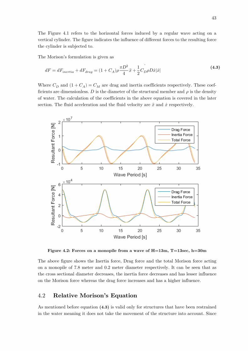
The Morison’s formulation is given as

𝑑𝑑𝐹𝐹 = 𝑑𝑑𝐹𝐹𝑖𝑖𝑛𝑛𝑖𝑖𝑟𝑟𝑖𝑖𝑖𝑖𝑎𝑎 + 𝑑𝑑𝐹𝐹𝑑𝑑𝑟𝑟𝑎𝑎𝑔𝑔 = (1 + 𝐶𝐶𝐴𝐴)𝜌𝜌 𝜋𝜋𝐷𝐷2

4𝜕𝜕 + 1

2𝐶𝐶𝐷𝐷𝜌𝜌𝐷𝐷𝜕𝜕|𝜕𝜕|

(4.3)

Where 𝐶𝐶𝐷𝐷 and (1 + 𝐶𝐶𝐴𝐴) = 𝐶𝐶𝑀𝑀 are drag and inertia coefficients respectively. These coef-ficients are dimensionless. 𝐷𝐷 is the diameter of the structural member and 𝜌𝜌 is the density of water. The calculation of the coefficients in the above equation is covered in the later section. The fluid acceleration and the fluid velocity are 𝜕𝜕 and 𝜕𝜕 respectively.

Figure 4.2: Forces on a monopile from a wave of H=13m, T=13sec, h=30m

The above figure shows the Inertia force, Drag force and the total Morison force acting on a monopile of 7.8 meter and 0.2 meter diameter respectively. It can be seen that as the cross sectional diameter decreases, the inertia force decreases and has lesser influence on the Morison force whereas the drag force increases and has a higher influence.

4.2 Relative Morison’s Equation

As mentioned before equation (4.3) is valid only for structures that have been restrained in the water meaning it does not take the movement of the structure into account. Since

44

in this project the movement of the structure is necessary in order to determine the most realistic forces, the Morison’s equation is reformulated to account for the relative velocities and accelerations. The hydrodynamic forces are calculated by using the second order theory for the regular waves and the first order theory for irregular waves.

Figure 4.3: Distributed Wave Loading on a Submerged Cylinder

Figure 4.3 shows the incoming wave acting on a structure. The distributed wave forces 𝑞𝑞𝑤𝑤𝑛𝑛

is dependent on the orientation of the beam and is perpendicular to the axis of the beam. The distributed wave loads are calculated using the relative Morison formula-tion as shown below

𝑞𝑞𝑤𝑤𝑛𝑛 = 𝐶𝐶𝑀𝑀𝜌𝜌𝑤𝑤𝐴𝐴��𝑢𝐹𝐹𝑛𝑛 − 𝜌𝜌𝑤𝑤𝐶𝐶𝐴𝐴𝐴𝐴��𝑢𝑆𝑆𝑛𝑛 + 12𝜌𝜌𝑤𝑤𝐶𝐶𝐷𝐷𝑛𝑛

𝐻𝐻𝑒𝑒𝑛𝑛|𝑒𝑒𝑛𝑛| (4.4)

Where, 𝐴𝐴 is the cross sectional area ��𝑢𝐹𝐹𝑛𝑛 is the fluid particle acceleration normal to the beam axis ��𝑢𝑆𝑆𝑛𝑛 is the structural acceleration normal to the beam axis 𝐶𝐶𝐴𝐴 is the added mass coefficient 𝑒𝑒𝑛𝑛 is the relative fluid structure velocity normal to the beam axis 𝐶𝐶𝐷𝐷𝑛𝑛

is the normal drag coefficient

Since the structure is damped in the Relative Morison Formula due to the added mass coefficient 𝐶𝐶𝐴𝐴, the use of additional hydrodynamic damping coefficients for the drag forces in the equation is not necessary. The relative fluid structure velocity is the difference between the fluid particle velocity and the structural velocity and the relative fluid struc-ture acceleration is the difference between the fluid particle acceleration and the structural acceleration shown in the equation below

𝑒𝑒𝑛𝑛 = 𝑢𝑢𝑖𝑖 − 𝜕𝜕𝑖𝑖 𝑒𝑒𝑖𝑖 = ��𝑢𝑖𝑖 − 𝜕𝜕��𝑖

(4.5)

45

The structural velocities are interpolated with the nodal velocities 𝒙𝒙 and the structural accelerations are interpolated with the nodal accelerations ��𝒙 as shown below

𝜕𝜕𝑖𝑖 = 𝑁𝑁𝑇𝑇 (𝜕𝜕𝑖𝑖)𝒙𝒙

𝜕𝜕��𝑖 = 𝑁𝑁𝑇𝑇 (𝜕𝜕��𝑖)��𝒙 (4.6)

The distributed wave loading 𝑞𝑞𝑤𝑤𝑡𝑡which is tangential to the beam axis is mainly due to

skin friction. Even though this tangential drag force is small compared to the normal drag force will have an important impact for long slender elements. The contribution from the distributed wave loading tangential to the beam axis 𝑞𝑞𝑤𝑤𝑡𝑡

is given as

𝑞𝑞𝑤𝑤𝑖𝑖 = 12𝜌𝜌𝑤𝑤𝐶𝐶𝐷𝐷𝑡𝑡

𝐻𝐻𝑒𝑒𝑖𝑖|𝑒𝑒𝑖𝑖| (4.7)

In which 𝐶𝐶𝐷𝐷𝑡𝑡 and 𝑒𝑒𝑖𝑖 are the tangential drag coefficient and the relative fluid structure

velocity tangential to the beam axis respectively. The calculation of the hydrodynamic coefficients of the structure is covered in the following section.

4.3 Calculation of Hydrodynamic Coefficients

The determination of hydrodynamic coefficients should be done before the calculation or analysis of the forces can be carried out. In the Morison equation there are two hydrody-namic coefficients namely the inertia coefficient 𝐶𝐶𝑀𝑀 and the drag coefficient 𝐶𝐶𝐷𝐷, whereas in the Relative Morison equation there is a third hydrodynamic coefficient namely the added mass coefficient 𝐶𝐶𝐴𝐴.

4.3.1 Drag and Inertia Coefficients

Offshore cylindrical structures are dominated by inertia and drag forces. If the cross sec-tion of the cylindrical structure are large then the forces would be inertia dominated due to wave diffraction but if the cross section of the cylindrical structure is small then the drag forces would have a higher impact compared to the inertia forces. This is shown in Figure 4.2. The Reynolds number 𝑅𝑅𝑖𝑖, the Keulegan-Carpenter Number 𝐾𝐾𝐶𝐶 and the roughness ∆ are the important parameters required for the determination of Drag and Inertia coefficients. These parameters are given as

𝑅𝑅𝑖𝑖 = 𝑢𝑢𝐷𝐷𝑣𝑣

𝐾𝐾𝐶𝐶 = 𝑢𝑢𝑚𝑚𝑇𝑇𝐷𝐷

∆= 𝑘𝑘𝐷𝐷

(4.8)

Where, 𝐷𝐷 is the diameter of the cylinder 𝑇𝑇 is the wave period 𝑘𝑘 is the surface roughness 𝑢𝑢 is the flow velocity 𝑣𝑣 is the fluid kinematic viscosity 𝑢𝑢𝑚𝑚 is the maximum orbital particle velocity

The inertia coefficient and the drag coefficient is given as

46

𝐶𝐶𝑀𝑀 = � 2.0 𝑓𝑓𝑓𝑓𝑒𝑒 𝐾𝐾𝐶𝐶 < 3max[2.0 − 0.044(𝐾𝐾𝐶𝐶 − 3); 1.6 − (𝐶𝐶𝐷𝐷𝑆𝑆 − 0.65)] 𝑓𝑓𝑓𝑓𝑒𝑒 𝐾𝐾𝐶𝐶 > 3

(4.9)

𝐶𝐶𝐷𝐷 = 𝐶𝐶𝐷𝐷𝑆𝑆 𝜓𝜓(𝐶𝐶𝐷𝐷𝑆𝑆,𝐾𝐾𝐶𝐶)

(4.10)

Where 𝐶𝐶𝐷𝐷𝑆𝑆 is the drag coefficient for the steady state which is given in equation (4.11) and 𝜓𝜓 is the wake amplification factor which is taken from Figure 4.4.

𝐶𝐶𝐷𝐷𝑆𝑆 =

⎩���⎨���⎧ 0.65 𝑓𝑓𝑓𝑓𝑒𝑒 𝑘𝑘

𝐷𝐷< 10−4(𝑎𝑎𝑚𝑚𝑓𝑓𝑓𝑓𝜕𝜕ℎ)

29 + 4 log (𝑘𝑘𝐷𝐷)

20𝑓𝑓𝑓𝑓𝑒𝑒 10−4 < 𝑘𝑘

𝐷𝐷< 10−2

1.05 𝑓𝑓𝑓𝑓𝑒𝑒 𝑘𝑘𝐷𝐷

> 10−2(𝑅𝑅𝑓𝑓𝑢𝑢𝑔𝑔ℎ)

(4.11)

The surface roughness 𝑘𝑘 is assumed to be smooth for uncoated and painted steel and if the surface is covered with marine growth, then it is chosen to between 0.005𝑚𝑚 − 0.05𝑚𝑚.

Figure 4.4: Wake Amplification Factor [15]

In the above figure the solid line is used if the surface is smooth and the dotted line is used if the surface is rough. For proper calculation the drag and inertia coefficients have to be calculated at each node and extraction point throughout every time step which would be time consuming. So, for the sake of simplification and to reduce the calculation time the drag and inertia coefficients are kept constant. For all the calculations in this project the drag coefficient 𝐶𝐶𝐷𝐷 is set to 0.5 and the inertia coefficient 𝐶𝐶𝑀𝑀 is set to 2 as per the recommendation of DNV.

4.3.2 Added Mass Coefficient

47

As mentioned before in the Relative Morison equation there is an extra coefficient called the Added Mass coefficient 𝐶𝐶𝐴𝐴. Due to the fluid acting on a body under water an addi-tional force has to be included in the analysis of the body’s motion in the waves. As the body moves in the fluid, an amount of fluid moves with it, i.e. the fluid accelerates as the body accelerates. Compared to vacuum more fore is required in fluids to accelerate a body. This additional force is given by the added mass and is calculated as

𝑚𝑚𝑎𝑎 = 𝜌𝜌𝜋𝜋𝑒𝑒2𝐿𝐿 (4.12) Where 𝑒𝑒 and 𝐿𝐿 are the radius and length of the cylinder respectively. The non-dimen-sional added mass coefficient 𝐶𝐶𝐴𝐴 is found by

𝐶𝐶𝐴𝐴 = 𝑚𝑚𝑎𝑎𝜌𝜌𝐴𝐴𝑠𝑠

(4.13)

Therefore as the body moves in the wave the amount of body submerged in water changes with time which changes the added mass coefficient.

48

5. Wave Load Modelling The wave kinematics obtained from Chapter 3 is applied in the relative Morison formu-lation in Chapter 4 to obtain the hydrodynamic forces which helps in determining the impact of wave loads on the floating space frame structure. As the hydrodynamic forces are given in differential form as a force per unit length, a transformation of the differential hydrodynamic forces into nodal loads is needed. This transformation is explained in this chapter and can be accomplished by the two following approaches.

• Numerical integration is introduced to transform the nodal forces into the hydro-dynamic forces, based on the trapezoidal rule and by means of numerical integra-tion.

• A higher order polynomial regression is used to represent the differential hydro-dynamic forces. These hydrodynamic forces are subsequently transformed into consistent beam loads by the interpolation function.

The projection of the kinematic quantities are described and explained in the present chapter and an explanation of the implementation of the above two mentioned methods for representing the hydrodynamic forces is followed.

5.1 Projection of the Kinematic Quantities

A transverse and a tangential force contribution is induced on each member of the floating space frame structure by the kinematic quantities. Depending on the angle of the member, either the difference or the sum of the projected horizontal and vertical components of the kinematic quantities are used to obtain the transverse and tangential force contribu-tion. The transformation matrix is used to represent the orientation of each of the member which is given as follows

�𝜕𝜕𝑙𝑙𝜕𝜕𝑙𝑙

� = � cos 𝜃𝜃 sin 𝜃𝜃− sin 𝜃𝜃 cos 𝜃𝜃� �𝑋𝑋𝑍𝑍� �𝑋𝑋𝑍𝑍� = �cos 𝜃𝜃 −sin 𝜃𝜃

sin 𝜃𝜃 cos 𝜃𝜃 � �𝜕𝜕𝑙𝑙𝜕𝜕𝑙𝑙

� (5.1)

The below figure shows the illustration of the projection of the kinematic quantities which has been implemented in MATLAB.

Figure 5.1: Projection of Kinematic Quantities [16]

49

In the calculation of the differential hydrodynamic forces by the means of the relative Morison’s formula, the transverse and the tangential contributions of the kinematic quan-tities has been applied and the obtained hydrodynamic forces are subsequently trans-formed into nodal loads. A satisfactory distribution of the hydrodynamic forces is needed in order to obtain an accurate transformation of the hydrodynamic forces into nodal loads. This distribution of the hydrodynamic forces is achieved by sufficiently discretising the beam. In order to reduce the computational time which is caused due to large discretisa-tion of the structure, extraction points have been introduced which is explained in the following section.

5.2 Extraction Points

Extra sub nodes are generated between the main nodes in order to ensure that a given structure has sufficient number of nodes. These nodes are also known as the extraction points. The below figure shows the illustration of a beam element with three extraction points.

Figure 5.2: A beam element with 3 extraction points

The number of extraction points needed to obtain a sufficient representation of the hy-drodynamic forces depends on the average length between all the connected main nodes in the structure and it also depends on the method which has been used to transform the forces into consistent nodal loads.

5.3 Polynomial Regression of Hydrodynamic Forces

A higher order polynomial regression is used to represent the differential hydrodynamic forces in this section. The type of load the structure is exposed to determines the degree of polynomial. A quadratic regression provides a decent fit to the hydrodynamic forces for a first order wave. The quadratic regression is written as

50

𝑝𝑝(𝜕𝜕) = 𝑝𝑝1𝜕𝜕2 + 𝑝𝑝2𝜕𝜕 + 𝑝𝑝3 (5.2) The coefficients 𝑝𝑝1 to 𝑝𝑝3 are obtained by using the function in MATLAB called Polyfit, where the input parameters are the differential hydrodynamic forces in the nodes and in the extraction points for each element, the distance between the nodes, the extraction points and the degree of the polynomial.

Transformation of Hydrodynamic forces into Beam Loads With the quadratic regression describing the distributed forces over the elements, the forces are now transformed into beam loads by means of the consistent load vectors. The consistent load vectors are defined via the integration of the product of the product of the transposed shape function 𝑁𝑁𝑇𝑇 and the polynomial loads 𝑝𝑝 over the length of the ele-ment 𝐿𝐿.

𝑒𝑒 = �𝑁𝑁𝑇𝑇 𝑝𝑝 𝑑𝑑𝐿𝐿 (5.3)

The consistent load vector contains a transverse load, a tangential load and a bending moment at each node of each element and is illustrated in the figure below

Figure 5.3: Transverse and Tangential loads and bending moments acting on two beam elements [16]

The last step of the transformation is the use of the transformation matrix for the pro-jection of the local loads to global loads.

5.4 Modelling of Self Weight

The loading obtained from the mass due to the acceleration of gravity has an impact on the floating space frame structure. The self-weight is implemented in the same manner as the hydrodynamic forces, namely by projection and transformation of the distributed self-

51

weight load to nodal loads. The self-weight load of the structure is separated into a trans-verse load and a tangential load by projection as shown in the below figure.

Figure 5.4: The loading obtained by the mass due to the gravity acceleration acting on the structure [16]

By application of the consistent load vectors, the distributed loads are transformed into beam loads and subsequently projected to global loads. The self-weight is included in all the wave analyses performed in the project.

5.5 Validation of the wave structure interaction

Figure 5.5: Model setup for calculation

The interaction between the wave and the structure is done by the use of the following example. The model is setup as shown in the figure above. The model is prevented from moving in the vertical direction i.e. a roller support is applied at the intersection of the two arms, point 1 and point 2. The displacement is calculated at point 1 and point 2

52

shown in the above figure and validated against ANSYS. A regular 1st order wave having a wave height of 7m and a time period of 11 sec is applied on the model.

Figure 5.6: Displacement comparison in x-direction between MATLAB and ANSYS

Figure 5.7: Displacement comparison in y-direction between MATLAB and ANSYS

The displacement obtained in the x-direction in ANSYS and MATLAB is shown in the Figure 5.6. The displacement obtained in the y-direction in Ansys and MATLAB is shown in the Figure 5.7. The displacement obtained in both x and y-direction in both ANSYS and MATLAB are the same and hence the code is validated. Appendix A5 contains the Ansys file used.

-0.3

-0.2

-0.1

0

0.1

0.2

0.3

0 5 10 15 20 25 30 35

Dis

plac

emen

t in

x-di

rect

ion

[m]

Time [sec]

MATLAB (x1) MATLAB (x2)

ANSYS (x1) ANSYS (x2)

-5-4.5

-4-3.5

-3-2.5

-2-1.5

-1-0.5

00.5

0 5 10 15 20 25 30 35

Dis

plac

emen

t in

y-di

rect

ion

[m]

Time [sec]

MATLAB (y1) MATLAB (y2) ANSYS (y1) ANSYS (y2)

53

5.6 Drift forces

The average over time of the 1st order waves loads on a structure is always equal to zero, if the loads are integrated to the mean load [22]. This is due to the fact that all the load components that are determined by the 1st order theory and the integration of all the wave loads stops at the mean water level (MWL). Drift forces are of major importance for the motions of a floating body.

Drift velocity is not present in the 1st order wave theory and hence for the model setup shown in Figure 5.6 the displacement obtained in Figure 5.8 will always be less than the displacement that will be obtained by use of a higher order theory. The figure below shows the comparison of the displacement obtained by the use of the 1st order regular wave theory and the 2nd order regular wave theory.

Figure 5.8: Displacement comparison in y-direction between the 1st order and the 2nd order theory

The displacement obtained in y-direction by the use of 1st order wave from both points 1 and point 2 lie on each other. The displacement obtained in y-direction by the use of the 2nd order wave at point 1 and point 2 lie on each other but show a greater displacement compared to the 1st order wave due to the presence of drift. The obtained displacement values are present in Appendix A6

-8

-7

-6

-5

-4

-3

-2

-1

0

1

0 5 10 15 20 25 30 35

Dis

plac

emen

t in

Y-di

rect

ion

Time

1st y1 1st y2 2nd y1 2nd y2

54

6. Floating Space Frame Structure In this present chapter the time-domain dynamic response of the floating space frame structure is explained and determined by SOFIA. The WEPTOS Floating Space Frame Structure that has been designed and used in this section is shown in Figure 6.1.

Figure 6.1: Floating Space Frame Structure

The detailed structure shown in Figure 6.1 and the anchoring rope with the cable speci-fication has not been possible to model in Ansys Workbench due to which no comparison of the predicted dynamic response of the floating space frame structure with the anchoring cable obtained from SOFIA is conducted. Instead the analyses have been performed with varying the stiffness of the node in the cable and the mooring line forces obtained from the 1st order regular wave and the 2nd order regular wave as well as the dynamic response of the floating space frame structure is compared. The modelling of the anchoring cable as well as the modelling of the boundary conditions in MATLAB have been described in the following subsections.

6.1 Modelling of Anchoring Cable

The anchoring cable supporting the floating space frame structure is modelled based on the product information catalogue given by the manufacturer Bridon [23]. The anchoring cables are modelled as circular cross-sectional solids and the moment of inertia of these anchoring cables are reduced so as to assume that these anchoring cables are flexible in bending, in which they possess only axial stiffness. These anchoring cables used in MATLAB are an approximation of a realistic anchoring cables.

55

Figure 6.2: Bridon Tiger Dyform 6R 6x36 Class [23]

The anchoring cable used for the space frame structure is a steel wire rope manufactured in a 6X36 wire lay construction as shown in Figure 6.2. The rope is designed for applica-tions of mooring lines. The diameter of the rope is 33𝑚𝑚𝑚𝑚 and having an approximate mass of 4.52𝑘𝑘𝑔𝑔/𝑚𝑚. The anchoring cable has a length of 25𝑚𝑚 and is divided into 25 element each having 1𝑚𝑚 length.

6.2 Modelling of the Space frame structure.

The WEPTOS space frame structure is modelled by cylinders having an inner diameter of 0.2𝑚𝑚 and an outer diameter of 0.23𝑚𝑚. To ensure floating the elements are modelled such that the buoyancy is always more than the weight of the elements. The Floating Space Frame Structure is shown in Figure 6.1 is a representation of the WEPTOS like Structure taken from the website [24]. It should be noted that since it was not possible to obtain the actual dimensions of the WEPTOS space frame structure, the dimensions used are only a physical representation and are not the actual dimensions.

The arms of the WEPTOS space frame structure has a length of 64𝑚𝑚. The angle between the two arms is of 60°. A simple connection instead of the actual connection is made between the two arms in order to simplify the design. The dimension of the connection has been increased in order to provide more buoyancy to the structure and increase its strength. An inner diameter of 0.33𝑚𝑚 and an outer diameter of 0.37𝑚𝑚 has been used for the connection.

6.3 Dynamic response of the Structure

The last element of the anchoring cable is fixed to prevent it from having displacement and moment in any of the 3 direction. Three different analyses have been performed by varying the stiffness of the second last element in the anchoring cable. The third last element in the anchoring cable represents the investigation point 1. Changing of the stiff-ness is an illustration of how the buoyancy of the buoy to which the anchoring cable is

56

supposed to be attached will affect the structure. The Figure 6.3 shows the modelled space frame structure and the points that have been investigated.

Figure 6.3: Investigation points in the Space Frame structure

A time domain analysis with a simulation duration of 30𝑎𝑎𝑒𝑒𝑐𝑐 and having a time step of 0.005𝑎𝑎𝑒𝑒𝑐𝑐 has been performed. The structure has a total of 463 beam elements due to which the computational time is very high. The floating space frame structure has been subjected to a regular first order wave and a regular second order wave having a wave height 𝐻𝐻 = 7𝑚𝑚, water depth ℎ = 30𝑚𝑚 and a wave period of 11𝑎𝑎𝑒𝑒𝑐𝑐. The location of this wave parameter is present in Figure 2.8. This wave parameter has been chosen as the second order regular wave theory is valid for this wave specification which can be calcu-lated from Figure 2.2 and it will be possible to see the variations that are obtained be-tween the wave theories. Mooring line forces at investigation point 1 are extracted in order to determine the forces to which the anchoring cable will be subjected to. The horizontal displacements in the y-direction and vertical displacements are extracted at both investigation point 1 and 2. The corresponding velocities and accelerations are pre-sent in the excel file in Appendix A7. The number 1st and 2nd are used to represent the 1st order regular wave and the 2nd order regular wave respectively in the upcoming figures.

57

Figure 6.4: Mooring line Force vs Time for stiffness reduced by 10%

Figure 6.4 shows mooring line force vs time plot obtained for reducing the stiffness of the mooring line at the point shown in Figure 6.3. The stiffness at the node in the mooring line is reduced by 10% i.e. only 90% of the total stiffness is acting at the specified point. The reduction of stiffness is an indirect illustration of the buoy being pulled by the space frame structure.

Figure 6.5: Mooring line Force vs Time for actual stiffness and stiffness increased by 10% at the node

-500000

0

500000

1000000

1500000

2000000

2500000

3000000

0 5 10 15 20 25 30 35

Moo

ring

Lin

e Fo

rce

[N]

Time [sec]

1st mooring 90% 2nd mooring 90%

-1000000

0

1000000

2000000

3000000

4000000

5000000

6000000

7000000

8000000

0 5 10 15 20 25 30 35

Moo

ring

Lin

e Fo

rce

[N]

Time [sec]

1st mooring 2nd mooring 1st mooring 110% 2nd mooring 110%

58

Figure 6.5 shows mooring line force vs time plot obtained for the actual stiffness and for increasing the stiffness of the mooring line at the point shown in Figure 6.3. It can be noticed from the figure that the mooring line force obtained when the 2nd order regular wave is acting on the model is higher than the mooring line force obtained when the model is subjected to a 1st order wave for the same stiffness. The peaks represents when the mooring line stretches and is in tension. The other parts of the figure represents when there is no tension on the mooring line and the mooring line is free. In theory it should be possible to see a constant tension on the mooring line for the 2nd order wave. But for this the analysis has to be carried out for a longer period of time.

Figure 6.6: Vertical displacement at investigation point 1 & 2 for varying stiffness

Figure 6.6 shows the vertical displacement vs time at the investigation point 1 and inves-tigation point 2. In the legend the letter ‘m’ is used to represent the mooring line i.e. the investigation point 1 and the letter ‘s’ is used to represent the structure i.e. the investi-gation point 2. As expected the vertical displacement at investigation point 1 which is present on the mooring line is far less compared to investigation point 2 which is on the structure. The vertical displacement of the investigation point 2 represents the floating of the structure on the acting wave and hence the structure moves along with the wave. It can be noticed that there is a peak in displacement once every 11sec which represents the wave time period in this case.

-5

-4

-3

-2

-1

0

1

2

3

4

5

0 5 10 15 20 25 30 35

Dis

plac

emen

t [m

]

Time [sec]

2nd zm 110% 2nd zm 90% 2nd zm 1st zm 110%

1st zm 90% 1st zm 1st zs 1st zs 90%

1st zs 110% 2nd zs 2nd zs 90% 2nd zs 110%

59

Figure 6.7: Horizontal displacement at investigation point 1 & 2 for varying stiffness

Figure 6.7 shows the horizontal displacement vs time at the investigation point 1 and investigation point 2. The horizontal displacement is in the y-direction which is along the direction of the wave. As expected there is not much displacement at investigation point 1 which represents the mooring line. In the graph at 15.83 sec and at 26.08 sec the dis-placement has increased for the 2nd order wave whereas it remains the same for the 1st order wave. This displacement from the 2nd order wave will tend to increase constantly if the analysis is carried out for longer periods of time which will lead to a constant tension on the mooring line.

-7

-6

-5

-4

-3

-2

-1

0

1

0 5 10 15 20 25 30 35D

ispl

acem

ent

[m]

Time [sec]

2nd ym 110% 2nd ym 90% 2nd ym 1st ym 110%

1st ym 90% 1st ym 1st ys 1st ys 90%

1st ys 110% 2nd ys 2nd ys 90% 2nd ys 110%

60

7. Conclusion The objective of this project is to investigate the mooring line forces and the dynamic response of the WEPTOS WEC when subjected to a linear wave theory and a 2nd order wave theory. Out of all the wave theories only the first order wave theory and the second order wave theory have been taken into account in this project. All the structural elements in the project are modelled by cylindrical beam elements. The calculations in the project are based on the co-rotational beam formulation and is done numerically. The implemen-tation of the co-rotational beam formulation allows the WEPTOS WEC and other float-ing structure to have large displacement and rotation.

In order to take into account the movement of the structure when subjected to waves, the relative Morison’s equation has been implemented. A submerged V-structure is sub-jected to a wave for validation of the wave structure interaction. The displacement ob-tained along the direction of the wave for this structure is more when it is subjected to a 2nd order wave theory compared to a first order wave theory.

An anchored floating space frame structure similar to the WEPTOS WEC is modelled and subjected to first order regular wave and a second order regular wave. The mooring line forces is higher for the 2nd order regular wave theory when compared to the 1st order regular wave theory. Similarly the displacement of the structure along the direction of the wave appears to be larger for the 2nd order wave theory. If the analysis is carried out for a longer period of time a constant tension on the mooring line can be obtained.

61

Bibliography

[1] U.S. National Renewable Energy Laboratory, “Ocean Energy Technology Overview,” DOE/GO-102009-2823, July 2009.

[2] Chris Woodford, “OTEC (Ocean Thermal Energy Conversion),” 2012. [Online]. Available: http://www.explain that stuff.com/how-otec-works.html.

[3] National Renewable Energy Labratory and Department of Energy, “Ocean Energy,” [Online]. Available: http://www.renewableenergyworld.com/ocean-energy/tech.html.

[4] Zhou Liu and Peter Frigaard, Generation and Analysis of Random Waves, Aalborg Universitet, January 2001.

[5] Se Joon Lim, “Wave Energy Convertors,” Stanford University, December 15, 2013.

[6] “Technology,” [Online]. Available: www.aquamarinepower.com.

[7] Arthur Pecher, “Performance Evaluation of Wave Energy Converters,” Aalborg University, Department of Civil Engineering, Aalborg, Denmark, October 2012.

[8] The Queen's University of Belfast, “Islay Limpet Wave Power Plant,” 1 November 1998 to 30 April 2002.

[9] Mike Mekhiche and Kathleen A Edwards, “Ocean Power Technologies Powerbuoy: System-level design, development and validation methodology,” Seattle, WA, 2014.

[10] [Online]. Available: wavestarenergy.com.

[11] A. Pecher, J. P. Kofoed and T. Larsen, “The extensive R&D behind the Weptos WEC,” Renewable Energies Offshore, no. ISBN: 978-1-138-02871-5, p. 351, 2015.

[12] Thomas Lykke Andersen, Peter Frigaard and Hans F. Burcharth, Lecture notes for the course in Water Wave Mechanics, Aalborg: Aalborg University, ISSN: 1901-7286, October 2014.

[13] Michael Brorsen, “Non-linear Waves,” Aalborg Universitet, ISSN: 1901-7286, Aalborg, 2007.

[14] Robert M. Sorensen, Basic Coastal Engineering, 3rd ed., Springer US, 2006.

[15] DNV-OS-J101, Design of Offshore Wind Turbine Structures, Det Norske Veritas AS, May 2014.

62

[16] A. Taha and A. Kadriu, “Nonlinear Time-domain Analysis of Floating <space Frame Structures,” 2015.

[17] DNV-RP-C205, Environmental Conditions and Environmental Loads, Det Norske Veritas AS, October 2010.

[18] George Z. Forristall, “Wave Crest Distributions: Observations and Second-Order Theory,” Journal of Physical Oceanography, pp. 1931-1943, 2000.

[19] M.B. van der Meulen, T. Ashuri, G.J.W. van Bussel and D.P. Molenaar, “Influence of Nonlinear Irregular Waves on the Fatigue Loads of an Offshore Wind Turbine,” Siemens Wind Power, Hague, Netherlands.

[20] Z. X. Li and L. Vu-Quoc, “A Mixed Co-rotational 3D Beam Element Formulation for Arbitrarily Large Rotations,” Advanced Steel Construction, vol. 6, no. 2, pp. 767-787, 2010.

[21] Louie L. Yaw, “2D Corotational Beam Formulation,” Walla Walla University, November 30, 2009.

[22] Michael Brorsen, “Slowly-varying 2. order Wave Forces on Large Structures,” Aalborg University, Aalborg, 2006.

[23] “Bridon,” [Online]. Available: http://www.bridon.com/usa/site/products/undergroundmining/tigerdyform6r6x36.php.

[24] “Kirt Thomsen Visual R&D Consultancy,” [Online]. Available: http://kirt-thomsen.com/WEPTOS-Investor-presentation-1. [Accessed 19 3 2016].

[25] Maarten De Rijcke, Thomas Lykke Andersen, Luca Martinelli, Barbara Zanuttigh, Jørgen Harch Nørgaard, Rodolfo Silva and Piero Roul, “Wave Energy Convertors,” 8 November 2013. [Online]. Available: http://www.coastalwiki.org/wiki/Wave_energy_converters.

[26] “Wave Power,” [Online]. Available: https://en.wikipedia.org/wiki/Wave_power.

[27] Arthur Pecher, Jens Peter Kofoed and Tommy Larsen, “Design Specifications for the Hanstholm WEPTOS Wave Energy Converter,” Energies, pp. 1001-1017, 2012.

63

Appendix This Appendix contains the expansion of the formulas mentioned in the above chapters.

First order regular wave Horizontal Velocity

𝑢𝑢(1) = 𝜕𝜕𝜑𝜑(1)

𝜕𝜕𝜕𝜕= 𝑎𝑎𝑔𝑔𝑘𝑘

𝜔𝜔cosh (𝑘𝑘(𝜕𝜕 + ℎ))

cosh (𝑘𝑘ℎ)cos (𝜔𝜔𝜕𝜕 − 𝑘𝑘𝜕𝜕)

Vertical Velocity

𝑤𝑤(1) = 𝜕𝜕𝜑𝜑(1)

𝜕𝜕𝜕𝜕= − 𝑎𝑎𝑔𝑔𝑘𝑘

𝜔𝜔sinh (𝑘𝑘(𝜕𝜕 + ℎ))

cosh (𝑘𝑘ℎ)sin (𝜔𝜔𝜕𝜕 − 𝑘𝑘𝜕𝜕)

Horizontal Acceleration

��𝑢(1) = 𝑑𝑑𝑢𝑢(1)

𝑑𝑑𝜕𝜕≈ 𝜕𝜕𝑢𝑢(1)

𝜕𝜕𝜕𝜕= −𝑎𝑎𝑔𝑔𝑘𝑘 cosh (𝑘𝑘(𝜕𝜕 + ℎ))

cosh (𝑘𝑘ℎ)sin (𝜔𝜔𝜕𝜕 − 𝑘𝑘𝜕𝜕)

Vertical Acceleration

��𝑤(1) = 𝑑𝑑𝑤𝑤(1)

𝑑𝑑𝜕𝜕≈ 𝜕𝜕𝑤𝑤(1)

𝜕𝜕𝜕𝜕= −𝑎𝑎𝑔𝑔𝑘𝑘 sinh (𝑘𝑘(𝜕𝜕 + ℎ))

cosh (𝑘𝑘ℎ)cos (𝜔𝜔𝜕𝜕 − 𝑘𝑘𝜕𝜕)

Second order regular wave Horizontal Velocity

𝑢𝑢(2) = 𝜕𝜕𝜑𝜑(2)

𝜕𝜕𝜕𝜕= 𝑢𝑢(1) − 3

32𝑐𝑐𝑘𝑘2𝐻𝐻2cosh (2𝑘𝑘(𝜕𝜕 + ℎ))

sinh4(𝑘𝑘ℎ)cos�2(𝜔𝜔𝜕𝜕 − 𝑘𝑘𝜕𝜕)� − 1

8𝑔𝑔𝐻𝐻2

𝑐𝑐ℎ

Vertical Velocity

𝑤𝑤(2) = 𝜕𝜕𝜑𝜑(2)

𝜕𝜕𝜕𝜕= 𝑤𝑤(1) + 3

32𝑐𝑐𝑘𝑘𝐻𝐻2sinh (2𝑘𝑘(𝜕𝜕 + ℎ))

sinh4(𝑘𝑘ℎ)sin�2(𝜔𝜔𝜕𝜕 − 𝑘𝑘𝜕𝜕)�

Horizontal Acceleration

��𝑢(2) = 𝑑𝑑𝑢𝑢(2)

𝑑𝑑𝜕𝜕≈ 𝜕𝜕𝑢𝑢(2)

𝜕𝜕𝜕𝜕= ��𝑢(1) + 3

32𝑐𝑐𝑘𝑘2𝜔𝜔𝐻𝐻2cosh (2𝑘𝑘(𝜕𝜕 + ℎ))

sinh4(𝑘𝑘ℎ)sin�2(𝜔𝜔𝜕𝜕 − 𝑘𝑘𝜕𝜕)�

Vertical Acceleration

��𝑤(2) = 𝑑𝑑𝑤𝑤(2)

𝑑𝑑𝜕𝜕≈ 𝜕𝜕𝑤𝑤(2)

𝜕𝜕𝜕𝜕= ��𝑤(1) + 3

32𝑐𝑐𝑘𝑘𝜔𝜔𝐻𝐻2sinh (2𝑘𝑘(𝜕𝜕 + ℎ))

sinh4(𝑘𝑘ℎ)cos�2(𝜔𝜔𝜕𝜕 − 𝑘𝑘𝜕𝜕)�

First order irregular wave

64

Horizontal Velocity

𝑢𝑢(1) = 𝜕𝜕𝜑𝜑(1)

𝜕𝜕𝜕𝜕= �−𝑏𝑏𝑛𝑛𝑘𝑘𝑛𝑛

cosh (𝑘𝑘𝑛𝑛(𝜕𝜕 + ℎ))cosh (𝑘𝑘𝑛𝑛ℎ)

cos (𝜔𝜔𝑛𝑛𝜕𝜕 − 𝑘𝑘𝑛𝑛𝜕𝜕 − 𝜗𝜗𝑛𝑛)𝑁𝑁

𝑛𝑛=1

Vertical Velocity

𝑤𝑤(1) = 𝜕𝜕𝜑𝜑(1)

𝜕𝜕𝜕𝜕= �𝑏𝑏𝑛𝑛𝑘𝑘𝑛𝑛

sinh (𝑘𝑘𝑛𝑛(𝜕𝜕 + ℎ))cosh (𝑘𝑘𝑛𝑛ℎ)

sin (𝜔𝜔𝑛𝑛𝜕𝜕 − 𝑘𝑘𝑛𝑛𝜕𝜕 − 𝜗𝜗𝑛𝑛)𝑁𝑁

𝑛𝑛=1

Horizontal Acceleration

��𝑢(1) = 𝑑𝑑𝑢𝑢(1)

𝑑𝑑𝜕𝜕≈ 𝜕𝜕𝑢𝑢(1)

𝜕𝜕𝜕𝜕= �𝑏𝑏𝑛𝑛𝑘𝑘𝑛𝑛𝜔𝜔𝑛𝑛

cosh (𝑘𝑘𝑛𝑛(𝜕𝜕 + ℎ))cosh (𝑘𝑘𝑛𝑛ℎ)

sin (𝜔𝜔𝑛𝑛𝜕𝜕 − 𝑘𝑘𝑛𝑛𝜕𝜕 − 𝜗𝜗𝑛𝑛)𝑁𝑁

𝑛𝑛=1

Vertical Acceleration

��𝑤(1) = 𝑑𝑑𝑤𝑤(1)

𝑑𝑑𝜕𝜕≈ 𝜕𝜕𝑤𝑤(1)

𝜕𝜕𝜕𝜕= �𝑏𝑏𝑛𝑛𝑘𝑘𝑛𝑛𝜔𝜔𝑛𝑛

sinh (𝑘𝑘𝑛𝑛(𝜕𝜕 + ℎ))cosh (𝑘𝑘𝑛𝑛ℎ)

sin (𝜔𝜔𝑛𝑛𝜕𝜕 − 𝑘𝑘𝑛𝑛𝜕𝜕 − 𝜗𝜗𝑛𝑛)𝑁𝑁

𝑛𝑛=1

Second order irregular wave The transfer function used in the second order amplitude is given as

𝐵𝐵𝑚𝑚𝑛𝑛+ = 1

4�𝐷𝐷𝑚𝑚𝑛𝑛

+ − (𝑘𝑘𝑚𝑚𝑘𝑘𝑛𝑛 − 𝑅𝑅𝑚𝑚𝑅𝑅𝑛𝑛)�𝑅𝑅𝑚𝑚𝑅𝑅𝑛𝑛

+ (𝑅𝑅𝑚𝑚 + 𝑅𝑅𝑛𝑛)�

𝐷𝐷𝑚𝑚𝑚𝑚+ =

��𝑅𝑅𝑚𝑚 + �𝑅𝑅𝑛𝑛���𝑅𝑅𝑛𝑛(𝑘𝑘𝑚𝑚2 − 𝑅𝑅𝑚𝑚

2 ) + �𝑅𝑅𝑚𝑚(𝑘𝑘𝑛𝑛2 − 𝑅𝑅𝑛𝑛

2)���𝑅𝑅𝑚𝑚 + �𝑅𝑅𝑛𝑛�2 − 𝑘𝑘𝑚𝑚𝑛𝑛

+ tanh(𝑘𝑘𝑚𝑚𝑛𝑛+ ℎ)

+2��𝑅𝑅𝑚𝑚 + �𝑅𝑅𝑛𝑛�2(𝑘𝑘𝑚𝑚𝑘𝑘𝑛𝑛 − 𝑅𝑅𝑚𝑚𝑅𝑅𝑛𝑛)��𝑅𝑅𝑚𝑚 + �𝑅𝑅𝑛𝑛�2 − 𝑘𝑘𝑚𝑚𝑛𝑛

+ tanh(𝑘𝑘𝑚𝑚𝑛𝑛+ ℎ)

𝐵𝐵𝑚𝑚𝑛𝑛− = 1

4�𝐷𝐷𝑚𝑚𝑛𝑛

− − (𝑘𝑘𝑚𝑚𝑘𝑘𝑛𝑛 + 𝑅𝑅𝑚𝑚𝑅𝑅𝑛𝑛)�𝑅𝑅𝑚𝑚𝑅𝑅𝑛𝑛

+ (𝑅𝑅𝑚𝑚 + 𝑅𝑅𝑛𝑛)�

𝐷𝐷𝑚𝑚𝑚𝑚− =

��𝑅𝑅𝑚𝑚 − �𝑅𝑅𝑛𝑛���𝑅𝑅𝑛𝑛(𝑘𝑘𝑚𝑚2 − 𝑅𝑅𝑚𝑚

2 ) − �𝑅𝑅𝑚𝑚(𝑘𝑘𝑛𝑛2 − 𝑅𝑅𝑛𝑛

2)���𝑅𝑅𝑚𝑚 − �𝑅𝑅𝑛𝑛�2 − 𝑘𝑘𝑚𝑚𝑛𝑛

− tanh(𝑘𝑘𝑚𝑚𝑛𝑛− ℎ)

+2��𝑅𝑅𝑚𝑚 + �𝑅𝑅𝑛𝑛�2(𝑘𝑘𝑚𝑚𝑘𝑘𝑛𝑛 − 𝑅𝑅𝑚𝑚𝑅𝑅𝑛𝑛)��𝑅𝑅𝑚𝑚 − �𝑅𝑅𝑛𝑛�2 − 𝑘𝑘𝑚𝑚𝑛𝑛

− tanh(𝑘𝑘𝑚𝑚𝑛𝑛− ℎ)

The reduced wave numbers and the difference and sum wave numbers are given as

𝑘𝑘𝑚𝑚𝑚𝑚− = |𝑘𝑘𝑚𝑚 − 𝑘𝑘𝑛𝑛|

𝑘𝑘𝑚𝑚𝑚𝑚+ = 𝑘𝑘𝑚𝑚 + 𝑘𝑘𝑛𝑛

𝜓𝜓𝑚𝑚 = 𝜔𝜔𝑚𝑚𝜕𝜕 − 𝑘𝑘𝑚𝑚𝜕𝜕 − 𝜗𝜗𝑚𝑚

65

𝑅𝑅𝑚𝑚 =𝜔𝜔𝑚𝑚

2

𝑔𝑔

∆𝜑𝜑(2)(𝜕𝜕, 𝜕𝜕) = 14

� ��𝑏𝑏𝑚𝑚𝑏𝑏𝑛𝑛cosh (𝑘𝑘𝑚𝑚𝑛𝑛

± (𝜕𝜕 + ℎ))cosh (𝑘𝑘𝑚𝑚𝑛𝑛

± ℎ)𝐷𝐷𝑚𝑚𝑛𝑛

±

(𝜔𝜔𝑚𝑚 ± 𝜔𝜔𝑛𝑛)sin(𝜓𝜓𝑚𝑚 ± 𝜓𝜓𝑛𝑛)�

𝑁𝑁

𝑛𝑛=1

𝑁𝑁

𝑚𝑚=1

Horizontal Velocity

𝑢𝑢(2) = 𝜕𝜕𝜑𝜑(2)

𝜕𝜕𝜕𝜕= 𝑢𝑢(1)

± 14

� ��𝑏𝑏𝑚𝑚𝑏𝑏𝑛𝑛(𝑘𝑘𝑚𝑚 ± 𝑘𝑘𝑛𝑛) cosh (𝑘𝑘𝑚𝑚𝑛𝑛± (𝜕𝜕 + ℎ))

cosh (𝑘𝑘𝑚𝑚𝑛𝑛± ℎ)

𝐷𝐷𝑚𝑚𝑛𝑛±

(𝜔𝜔𝑚𝑚 ± 𝜔𝜔𝑛𝑛)cos(𝜓𝜓𝑚𝑚 ± 𝜓𝜓𝑛𝑛)�

𝑁𝑁

𝑛𝑛=1

𝑁𝑁

𝑚𝑚=1

Vertical Velocity

𝑤𝑤(2) = 𝜕𝜕𝜑𝜑(2)

𝜕𝜕𝜕𝜕= 𝑤𝑤(1) + 1

4� ��𝑏𝑏𝑚𝑚𝑏𝑏𝑛𝑛𝑘𝑘𝑚𝑚𝑛𝑛

± sinh (𝑘𝑘𝑚𝑚𝑛𝑛± (𝜕𝜕 + ℎ))

cosh (𝑘𝑘𝑚𝑚𝑛𝑛± ℎ)

𝐷𝐷𝑚𝑚𝑛𝑛±

(𝜔𝜔𝑚𝑚 ± 𝜔𝜔𝑛𝑛)sin(𝜓𝜓𝑚𝑚 ± 𝜓𝜓𝑛𝑛)�

𝑁𝑁

𝑛𝑛=1

𝑁𝑁

𝑚𝑚=1

Horizontal Acceleration

��𝑢(2) = 𝑑𝑑𝑢𝑢(2)

𝑑𝑑𝜕𝜕≈ 𝜕𝜕𝑢𝑢(2)

𝜕𝜕𝜕𝜕= ��𝑢(1)

± 14

� ��𝑏𝑏𝑚𝑚𝑏𝑏𝑛𝑛(𝑘𝑘𝑚𝑚 ± 𝑘𝑘𝑛𝑛)(𝜔𝜔𝑚𝑚

𝑁𝑁

𝑛𝑛=1

𝑁𝑁

𝑚𝑚=1

± 𝜔𝜔𝑛𝑛) cosh (𝑘𝑘𝑚𝑚𝑛𝑛± (𝜕𝜕 + ℎ))

cosh (𝑘𝑘𝑚𝑚𝑛𝑛± ℎ)

𝐷𝐷𝑚𝑚𝑛𝑛±

(𝜔𝜔𝑚𝑚 ± 𝜔𝜔𝑛𝑛)sin(𝜓𝜓𝑚𝑚 ± 𝜓𝜓𝑛𝑛)�

Vertical Acceleration

��𝑤(2) = 𝑑𝑑𝑤𝑤(2)

𝑑𝑑𝜕𝜕≈ 𝜕𝜕𝑤𝑤(2)

𝜕𝜕𝜕𝜕= ��𝑤(1)

+ 14

� ��𝑏𝑏𝑚𝑚𝑏𝑏𝑛𝑛𝑘𝑘𝑚𝑚𝑛𝑛± (𝜔𝜔𝑚𝑚

𝑁𝑁

𝑛𝑛=1

𝑁𝑁

𝑚𝑚=1

± 𝜔𝜔𝑛𝑛) sinh (𝑘𝑘𝑚𝑚𝑛𝑛± (𝜕𝜕 + ℎ))

cosh (𝑘𝑘𝑚𝑚𝑛𝑛± ℎ)

𝐷𝐷𝑚𝑚𝑛𝑛±

(𝜔𝜔𝑚𝑚 ± 𝜔𝜔𝑛𝑛)cos(𝜓𝜓𝑚𝑚 ± 𝜓𝜓𝑛𝑛)�