1

C. F. Jeff WuSchool of Industrial and Systems Engineering

Georgia Institute of Technology

Post-Fisherian Experimentation:from Physical to Virtual

•Fisher’s legacy in experimental design.•Post-Fisherian work in Factorial experiments: principles for factorial effects. conditional main effect analysis.

•Computer (virtual) experiments: numerical approach. stochastic approach via kriging.

•Summary remarks.

R. A. Fisher and his legacy

• In Oct 1919, Fisher joined RothamstedExperimental Station. His assignment was to “examine our data and elicit further information that

we had missed.” (by John Russell, Station Director )

• And the rest is history!

• By 1926 (a mere 7 years), Fisher had invented ANalysis Of VAriance and Design Of Experiments as new methods to design and analyze agricultural experiments.

2

Fisher’s Principles in Design

• Replication: to assess and reduce variation.

• Blocking.

• Randomization.

“Block what you can,

and randomize what you cannot.”

• Originally motivated by agricultural expts, have been widely used for any physical expts.

3

Factorial Experiments

• Factorial arrangement to accommodate factorial structure of treatment/block, by Fisher (1926) . Originally called “complex experiments”.

• Major work on factorial design by F. Yates (1935, 1937), and fractional factorials by D. Finney (1945); both worked with Fisher.

• Major development after WWII for applications to industrial experiments, by the Wisconsin School, G. Box and co-workers (J. S. Hunter, W. G. Hunter).

• What principles should govern factorial experiments?

4

Guiding Principles for Factorial Effects

• Effect Hierarchy Principle:

– Lower order effects more important than higher order effects;

– Effects of same order equally important.

• Effect Sparsity Principle: Number of relatively important effects is small.

• Effect Heredity Principle: for an interaction to be significant, at least one of its parent factors should be significant.

(Wu-Hamada book “Experiments”, 2000, 2009)5

Effect Hierarchy Principle

• First coined in Wu-Hamada book; was known in early work in data analysis.

• “From physical considerations and practical experience, (interactions) may be expected to be small in relation to error - - “ (Yates, 1935); “higher-order interactions - -are usually of less interest than the main effects and interactions between two factors only.” (Yates, 1937).

• The more precise version is used in choosing optimal fractions of designs; it can be used to justify maximum resolution criterion (Box-Hunter, 1961) and minimum aberration criterion (Fries-Hunter, 1980).

6

Effect Heredity Principle

• Coined by Hamada-Wu (1992); originally used to rule out incompatible models in model search.

• Again it was known in early work and used for analysis: “- - factors which produce small main effects usually show no significant interactions.” p.12 of Yates (1937): “The design and analysis of factorial experiments”,

Imperial Bureau of Soil Science, No. 35.

7

More on Heredity Principle

• Strong (both parents) and weak (single parent) versions defined by Chipman (1996) in bayesian framework. Strong heredity is the same as the marginality principle by McCullagh-Nelder (1989) but with different motivations.

• Original motivation in HW: application to analysis of experiments with complex aliasing.

8

9

Design Matrix OA(12, 27) and Cast Fatigue Data

Full Matrix: )2,12( 11OA

10

Partial and Complex Aliasing• For the 12-run Plackett-Burman design OA(12, 211)

partial aliasing: coefficient

complex aliasing: partial aliases.

• Traditionally complex aliasing was considered to be a disadvantage (called “hazards” by C. Daniel).

• Standard texts pay little attention to this type of designs.

ikj

jkii

,3

1 ˆE

3

1

)2

10 ( 45

Analysis Strategy

• Use effect sparsity to realize that the size of true model(s) is much smaller than the nominal size.

• Use effect heredity to rule out many incompatible models in model search.

• Frequentist version by Hamada-Wu (1992); Bayesian version by Chipman (1996)

• Effective if the number of significant interactions is small.

11

12

• Cast Fatigue Experiment:Main effect analysis: F (R2=0.45)

F, D (R2=0.59)HW analysis: F, FG (R2=0.89)

F, FG, D (R2=0.92)•Blood Glucose Experiment (3-level factors):

Main effect analysis: Eq, Fq (R2=0.36)HW analysis: Bl, (BH)lq, (BH)qq (R2=0.89)

•Bayesian analysis also identifies Bl, (BH)ll, (BH)lq, (BH)qq as having the highest posterior model probability.

Analysis Results

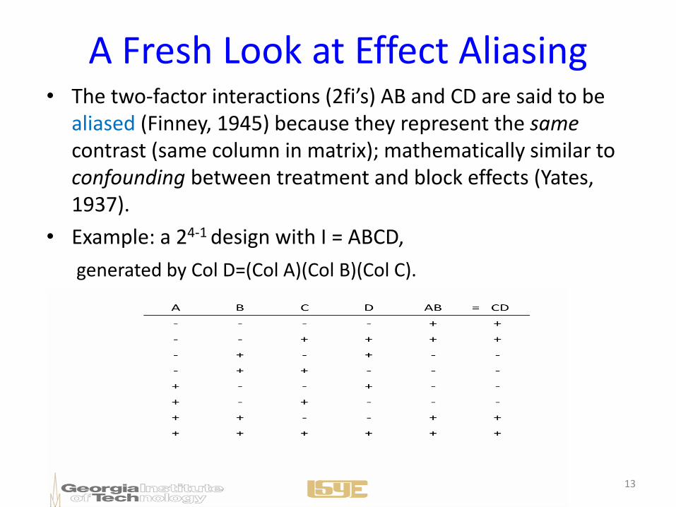
A Fresh Look at Effect Aliasing• The two-factor interactions (2fi’s) AB and CD are said to be

aliased (Finney, 1945) because they represent the samecontrast (same column in matrix); mathematically similar to confounding between treatment and block effects (Yates, 1937).

• Example: a 24-1 design with I = ABCD,

generated by Col D=(Col A)(Col B)(Col C).

13

De-aliasing of Aliased Effects

• The pair of effects cannot be disentangled, and are `thus not estimable. They are said to be fully aliased.

• Can they be de-aliased without adding runs??

• Hint: an interaction, say AB, should be viewed `together with its parent effects A and B.

• Approach: view AB as part of the 3d space of A, B, `AB; similarly for C, D, CD; because AB=CD, joint ` ` ` `space has 5 dimensions, not 6; then reparametrize`each 3d space.

14

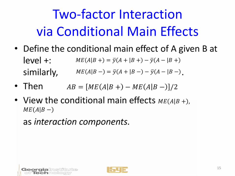
Two-factor Interaction via Conditional Main Effects

15

De-aliasing via CME Analysis

• Reparametrize the 3d space as A, B|A+, B|A-; the three effects are orthogonal but not of same length; similarly, we have C, D|C+, D|C-; in the joint 5d space, some effects are not orthogonal some conditional main effects (CME) can be estimated via variable selection, call this the CME Analysis.

• Non-orthogonality is the saving grace.

• Potential applications to social and medicalstudies which tend to have fewer factors.

16

Matrix Representation

• For the 24-1design with I = ABCD

17

A B C D B|A+ B|A- D|C+ D|C-

- - - - 0 - 0 -

- - + + 0 - + 0

- + - + 0 + 0 +

- + + - 0 + - 0

+ - - + - 0 0 +

+ - + - - 0 - 0

+ + - - + 0 0 -

+ + + + + 0 + 0

Car marriage station simulation experiment(GM, Canada, 1988)

18

DataFactors

yA B C D E F

- - - - - - 13+ + - - - - 5- - + - + - 69- - - + - + 16+ - + + - - 5+ - + - - + 7+ - - + + - 69+ - - - + + 69- + + + - - 9- + + - - + 11- + - + + - 69- + - - + + 89+ + + - + - 67+ + - + - + 13- - + + + + 66+ + + + + + 56

19

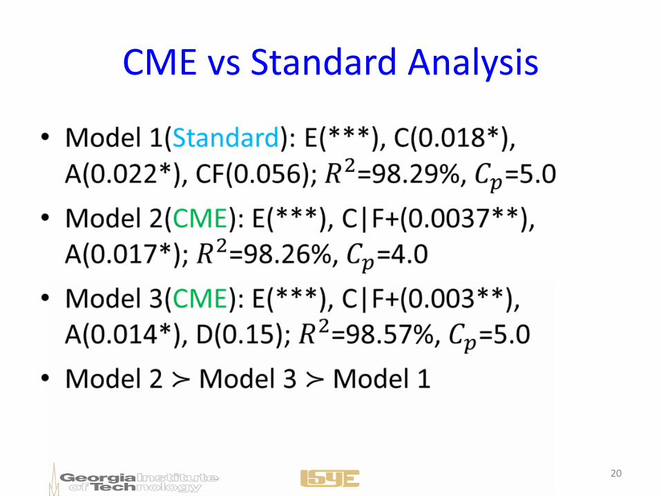
CME vs Standard Analysis

20

Interpretation of C|F+

• Lane selection C has a significant effect for larger cycle time F+, a more subtle effect than the obvious effect of E (i.e., % repair affects throughput).

21

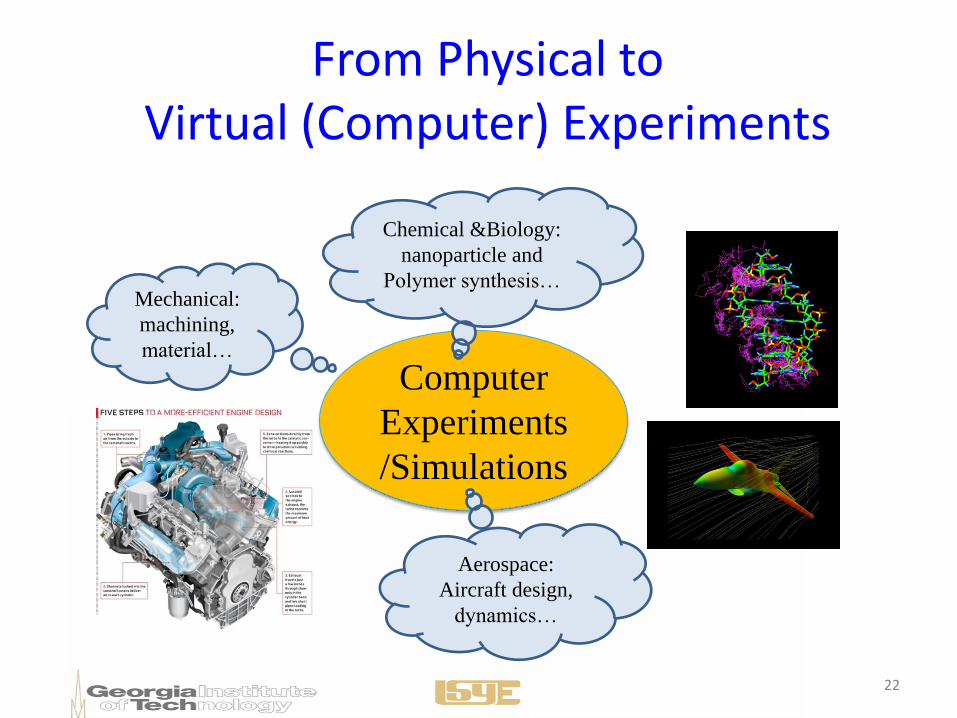
Computer

Experiments

/Simulations

Aerospace:

Aircraft design,

dynamics…

Mechanical:

machining,

material…

Chemical &Biology:

nanoparticle and

Polymer synthesis…

From Physical to Virtual (Computer) Experiments

22

Example of Computer Simulation:Designing Cellular Heat Exchangers

W

H

D

w1 w2 w3 wNh. . .

h2

h1

hNv

th

tv

Heat

Source

Tsource

Air Flow, Tin

.

.

.

x

y

z

Important Factors

• Cell Topologies, Dimensions, and Wall Thicknesses

• Temperatures of Air Flow and Heat Source

• Conductivity of Solid

• Total Mass Flowrate of Air

Response

• Maximum Total Heat Transfer

23

Heat Transfer Analysis

ASSUMPTIONS

–Forced Convection

–Laminar Flow: Re < 2300

–Fully Developed Flow

–Three Adiabatic (Insulated) Sides

–Constant Temperature Heat

Source on Top

–Fluid enters with Uniform Temp

–Flowrate divided among cells

*B. Dempsey, D.L. McDowell

ME, Georgia Tech

GOVERNING EQUATIONS

c s c c cT

Q k A A q in wallsx

h h h hQ hA T A q convection from walls to fluid

f pQ mc T fluid heating

24

Heat Transfer AnalysisA Detailed Simulation Approach--FLUENT

• FLUENT solves fluid flow and heat transfer problems with a computational fluid dynamics (CFD) solver.

• Problem domain is divided into thousands or millions of elements.

• Each simulation requires hours to days of computer time on a Pentium 4 PC.

FLUENT

25

Why Computer Experiments?• Physical experiments can be time-consuming, costly or

infeasible (e.g., car design, traffic flow, forest fire).

• Because of advances in numerical modeling and computing speed, computer modeling is commonly used in many investigations.

• A challenge: Fisher’s principles not applicable to deterministic (or even stochastic) simulations. Call for new principles!

• Two major approaches to modeling computer expts:

– stochastic modeling, primarily the kriging approach,

– numerical modeling.

26

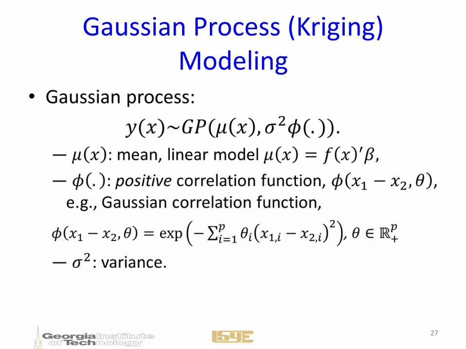
Gaussian Process (Kriging) Modeling

27

Kriging Predictor

28

0 0.2 0.4 0.6 0.8 1-1

-0.5

0

0.5

1

1.5

Kriging Predictor

Data

True Function

95% Confidence Interval

0 0.2 0.4 0.6 0.8 1-1

-0.5

0

0.5

1

1.5

New Kriging Predictor

Data

True Function

New Data

Old Kriging Predictor

95% Confidence Interval

Kriging as Interpolator and Predictor

29

Statistical Surrogate Modeling of Computer Experiments

prediction, optimization

surrogate model(Kriging)

computer modeling(finite-element simulation)

physical experiment or observations

more FEA runs

30

More on Kriging

31

Interplay Between Design and Modeling

• Computer simulations with different levels of accuracy (Kennedy-O’Hagan, 2000; Qian et al., 2006; Qian-Wu, 2008)

construction of nested space-filling (e.g., Latin hypercube) designs (Qian-Ai-Wu, 2009, various papers by Qian and others, 2009-date).

• GP model with quantitative and qualitativefactors (Qian-Wu-Wu, 2008, Han et al., 2009)

construction of sliced space-filling (e.g., Latin hypercube) designs (Qian-Wu, 2009, Qian, 2010).

32

Numerical Approach

• Can provide faster and more stable computation, and fit non-stationary surface with proper choice of basis functions.

• Some have inferential capability: Radial Basis interpolating Functions (closely related to kriging), smoothing splines (Bayesian interpretation).

• Others do not: MARS, Neural networks, regression-based inverse distance weighting interpolator (var est, but no distribution), sparse representation from overcompletedictionary of functions. Need to impose a stochastic structure to do Uncertainty Quantification. One approach discussed next.

33

Uncertainty Quantification

Prediction

Surrogate model(Kriging)

computer modeling(finite-element simulation)

Physical experiment or observations

UQ

UQ

34

35

Response Surface for Bistable Laser Diodes

1pS

cm

Scientific Objectives in Laser Diode Problem

• Each PLE corresponds to a chaotic light output, which can accommodate a secure optical communication channel; finding more PLEs would allow more secure communication channels.

• Objectives: Search all possible PLE (red area) and obtain predicted values for PLEs.

• A numerical approach called OBSM (next slide) can do this. Question: how to attach error limits to the predicted values?

36

Overcomplete Basis Surrogate Model

• Use an overcomplete dictionary of basis functions, no unknown parameters in basis functions.

• Use linear combinations of basis functions to approximate unknown functions; linear coefficients are the only unknown parameters.

• Use Matching Pursuit to identify nonzero coefficients; for fast and greedy computations.

• Choice of basis functions to “mimic” the shape of the surface. Can handle nonstationarity.

Chen, Wang, and Wu (2010)

37

Imposing a Stochastic Structure

38

Simulation Results I

Comparison between MP and SSVS

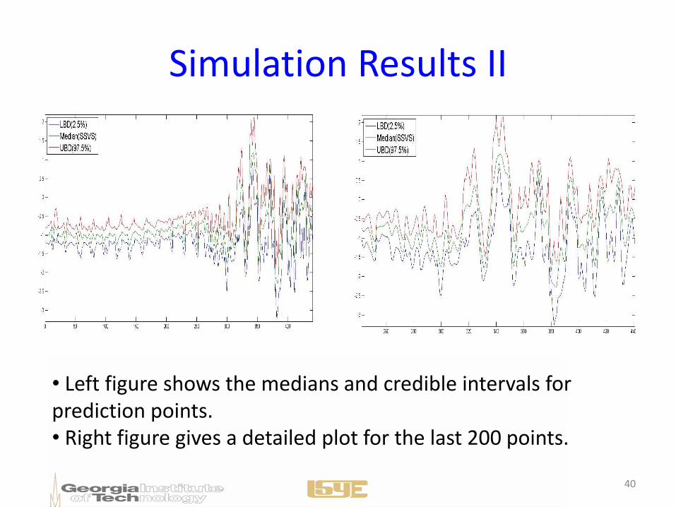
Simulation Results II

• Left figure shows the medians and credible intervals for prediction points.• Right figure gives a detailed plot for the last 200 points.

40

Summary Remarks

• Fisher’s influence continued from agricultural expts to industrial expts; motivated by the latter, new concepts (e.g., hierarchy, sparsity, heredity) and methodologies (e.g., response surface methodology, parameter design) were developed, which further his legacy.

• Because Fisher’s principles are less applicable to virtual experiments, we need new guiding principles.– Kriging can have numerical problems; tweaking or new

`stochastic approach?

– Numerical approach needs Uncertainty Quantification, a `new opportunity between stat and applied math.

– Design construction distinctly different from physical expts; `need to exploit its interplay with modeling.

41