Embed Size (px)
Citation preview
The Environmental Fluid Dynamics Code Theory and Computation
Volume 2: Sediment and Contaminant Transport and Fate
Tetra Tech, Inc. 10306 Eaton Place
Suite 340 Fairfax, VA 22030
June 2007
EFDC Sediment and Contaminant Theory and Computation
2
Preface
This document comprises the second volume of the theoretical and computational
documentation for the Environmental Fluid Dynamics Code (EFDC). The material in
this volume was previously distributed as:
Tetra Tech, 2002: EFDC Technical Memorandum: Theoretical and Computational
Aspects of Sediment and Contaminant Transport in the EFDC Model. Fairfax, VA.
.
EFDC Sediment and Contaminant Theory and Computation
3
Acknowledgements
The Environmental Fluid Dynamics Code (EFDC) is a public domain, open source,
surface water modeling system, which includes hydrodynamic, sediment and
contaminant, and water quality modules fully integrated in a single source code
implementation. EFDC has been applied to over 100 water bodies including rivers, lakes,
reservoirs, wetlands, estuaries, and coastal ocean regions in support of environmental
assessment and management and regulatory requirements.
EFDC was originally developed at the Virginia Institute of Marine Science (VIMS) and
School of Marine Science of The College of William and Mary, by Dr. John M. Hamrick
beginning in 1988. This activity was supported by the Commonwealth of Virginia
through a special legislative research initiative. Dr. Robert Byrne, the late Dr. Bruce
Neilson, and Dr. Albert Kuo of VIMS are acknowledged for their efforts in supporting
the original development activity. Subsequent support for EFDC development at VIMS
was provided by the U.S. Environmental Protection Agency and the National Oceanic
and Atmospheric Administration’s Sea Grant Program. The contributions of VIMS staff
and former students including Mr. Gamble Sisson, Dr. Zaohqing Yang, Dr. Keyong Park,
Dr. Jian Shen, and Dr. Sarah Rennie are gratefully acknowledged.
Tetra Tech, Inc. (Tt) became the first commercial user of EFDC in the early 1990’s and
upon Dr. Hamrick’s joining Tetra Tech in 1996, the primary location for the continued
development of EFDC. Tetra Tech has provided considerable internal research and
development support for EFDC over the past 10 years and Mr. James Pagenkopf, Dr.
Mohamed Lahlou, and Dr. Leslie Shoemaker are gratefully acknowledged for this. Mr.
Michael Morton of Tetra Tech is particularly recognized for his many contributions to
EFDC development and applications. The efforts Tetra Tech colleagues including Dr.
Jeff Ji, Dr. Hugo Rodriguez, Mr. Steven Davie, Mr. Brain Watson, Dr. Ruiz Zou, Dr. Sen
Bai, Dr. Yuri Pils, Mr. Peter von Lowe, Mr. Will Anderson, and Dr. Silong Lu are also
recognized. Their wide-ranging applications of EFDC have contributed to the robustness
of the model and lead to many enhancements.
Primary external support of both EFDC development and maintenance and applications
at Tetra Tech over the past 10 years has been generously provided by the U. S.
Environmental Protection Agency including the Office of Science and Technology, the
Office of Research and Development and Regions 1 and 4. In particular, Dr. Earl Hayter
(ORD), Mr. James Greenfield (R4), Mr. Tim Wool (R4) and Ms. Susan Svirsky (R1) are
recognized for their contributions in managing both EFDC developmental and application
work assignments.
The ongoing evolution of the EFDC model has to a great extent been application driven
and it is appropriate to thank Tetra Tech’s many clients who have funded EFDC
applications over the past 10 years. The benefits of ongoing interaction with a diverse
group of EFDC users in the academic, governmental, and private sectors are also
acknowledged.
EFDC Sediment and Contaminant Theory and Computation
4
Table of Contents
Preface
2
Acknowledgements
3
Contents
4
List of Figures
5
1. Introduction
6
2. Summary of Hydrodynamic and Generic Transport Formulations
7
3. Solution of the Sediment Transport Equation
13
4. Hydrodynamic and Sediment Boundary Layers
16
5. Sediment Bed Mass Conservation and Geomechanics
39
6. Noncohesive Sediment Settling, Deposition and Resuspension
56
7. Cohesive Sediment Settling, Deposition and Resuspension
68
8. Sorptive Contaminant Transport
75
9. References
91
EFDC Sediment and Contaminant Theory and Computation
5
List of Figures
Page
5.1
Specific Weight Normalized Effective Stress Versus Void Ratio 54
5.2
Compress Length Scale, ( ) ( )
1/
w eg d dρ σ ε
−, Versus Void Ratio. 54
5.3
Hydraulic Conductivity Versus Void Ratio 55
5.4
Hydraulic Conductivity/(1 + Void Ratio) Versus Void Ratio 55
6.1 Critical Shield's shear velocity and settling velocity as a function
of sediment grain size 67
EFDC Sediment and Contaminant Theory and Computation
6
1. Introduction
This report summarizes theoretical and computational aspects of the sediment and
sorptive contaminant transport formulations used in the EFDC model. Theoretical and
computational aspects for the basic EFDC hydrodynamic and generic transport model
components are presented in Hamrick (1992). Theoretical and computational aspects of
the EFDC water quality-eutrophication model component are presented in Park et al.
(1995). The paper by Hamrick and Wu (1997) also summarized computational aspects of
the hydrodynamic, generic transport and water quality-eutrophication components of the
EFDC model. The EFDC model has been extensively applied to estuaries (Fredricks and
Hamrick, 1996; Shen and Kuo, 1999; Shen et al., 1999; Ji et al., 2001), lakes (Jin et al.,
2000; 2002), reservoirs (Hamrick and Mills, 2000), rivers (Ji et al., 2002), and wetlands
(Moustafa and Hamrick, 2000). The model has also been used for a number of
fundamental process studies (Hamrick, 1994; Kuo et al., 1996; Yang et al., 2000).
This report is organized as follows. Chapter 2 summarizes the hydrodynamic and generic
transport formulations used in EFDC. Chapter 3 summarizes the solution of the transport
equation for suspended cohesive and noncohesive sediment. A discussion of near bed
boundary layer processes relevant to sediment transport is presented in Chapter 4.
Sediment bed mass conservation and methods for representation of the bed’s
geomechanical properties are discussed in Chapter 5. Chapters 6 and 7 summarize
noncohesive and cohesive sediment settling, deposition and resuspension process
representations. The final chapter, Chapter 9, documents the EFDC model's sorptive
contaminant transport and fate formulations.
EFDC Sediment and Contaminant Theory and Computation
7
2. Summary of Hydrodynamic and Generic Transport
Formulations
This section summarizes the hydrodynamic and transport equations used by the EFDC
model. Reference is made to Hamrick (1992), Hamrick and Wu (1997) and Tetra Tech
(2007a) for details of the computational procedure. This section does however describe
modifications to the solution procedure when the model operates in a geomorphologic
mode.
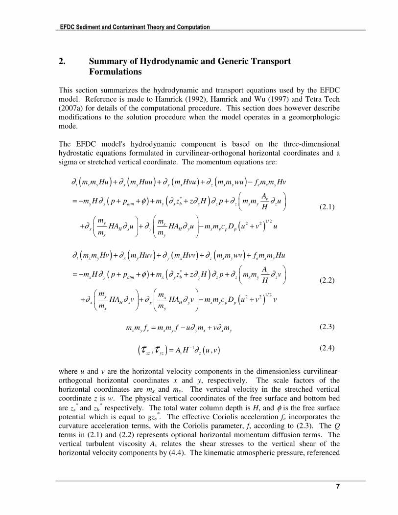
The EFDC model's hydrodynamic component is based on the three-dimensional
hydrostatic equations formulated in curvilinear-orthogonal horizontal coordinates and a
sigma or stretched vertical coordinate. The momentum equations are:
( ) ( ) ( ) ( )
( ) ( )
( )
*
1/ 22 2
t x y x y y x z x y e x y
vy x atm y x b x z z x y z
y xx H x y H y x y p p
x y
m m Hu m Huu m Hvu m m wu f m m Hv
Am H p p m z z H p m m u
H
m mHA u HA u m m c D u v u
m m
∂ ∂ ∂ ∂
∂ φ ∂ ∂ ∂ ∂ ∂
∂ ∂ ∂ ∂
+ + + −
= − + + + + +
+ + − +
(2.1)
( ) ( ) ( ) ( )
( ) ( )
( )
*
1/ 22 2
t x y x y y x z x y e x y
vx y atm x y b y z z x y z
y xx H x y H y x y p p
x y
m m Hv m Huv m Hvv m m wv f m m Hu
Am H p p m z z H p m m v
H
m mHA v HA v m m c D u v v
m m
∂ ∂ ∂ ∂
∂ φ ∂ ∂ ∂ ∂ ∂
∂ ∂ ∂ ∂
+ + + +
= − + + + + +
+ + − +
(2.2)
x y e x y y x x ym m f m m f u m v m∂ ∂= − + (2.3)
( ) ( )1, ,xz yz v z
A H u v∂τ τ −= (2.4)
where u and v are the horizontal velocity components in the dimensionless curvilinear-
orthogonal horizontal coordinates x and y, respectively. The scale factors of the
horizontal coordinates are mx and my. The vertical velocity in the stretched vertical
coordinate z is w. The physical vertical coordinates of the free surface and bottom bed
are zs*
and zb* respectively. The total water column depth is H, and φ is the free surface
potential which is equal to gzs*. The effective Coriolis acceleration fe incorporates the
curvature acceleration terms, with the Coriolis parameter, f, according to (2.3). The Q
terms in (2.1) and (2.2) represents optional horizontal momentum diffusion terms. The
vertical turbulent viscosity Av relates the shear stresses to the vertical shear of the
horizontal velocity components by (4.4). The kinematic atmospheric pressure, referenced
EFDC Sediment and Contaminant Theory and Computation
8
to water density, is patm, while the excess hydrostatic pressure in the water column is
given by:
( ) 1
z o op gHb gH∂ ρ ρ ρ −= − = − − (2.5)
where ρ and ρo are the actual and reference water densities and b is the buoyancy. The
horizontal turbulent stress on the last lines of (2.1) and (2.2), with AH being the horizontal
turbulent viscosity, are typically retained when the advective acceleration are represented
by central differences. The last terms in (2.1) and (2.2) represent vegetation resistance
where cp is a resistance coefficient and Dp is the dimensionless projected vegetation area
normal to the flow per unit horizontal area.
The three-dimensional continuity equation in the stretched vertical and curvilinear-
orthogonal horizontal coordinate system is:
( ) ( ) ( ) ( ) ( )( )0t x y x y y x z x y H SS SW
m m H m Hu m Hv m m w Q Q Q∂ ∂ ∂ ∂ δ+ + + = + + (2.6)
with QH representing volume sources and sinks including rainfall, evaporation, and lateral
inflows and outflows having negligible momentum fluxes. The terms QSS and QSW are
the net volumetric fluxes of sediment and water between the bed and water column,
defined as positive from the bed to the water column, when the model operates in a
geomorphologic mode. The delta function, δ(0) indicates these fluxes enter the bottom
layer of the water column. Integration of (2.6) over the depth gives
( ) ( ) ( )t x y x y y x H SS SWm m H m Hu m Hv Q Q Q∂ ∂ ∂+ + = + + (2.7)
In the geomorphologic mode, the water column continuity equation is coupled to a bulk
volume conservation equation for the sediment bed.
( )t x y GW SS SWm m B Q Q Q∂ = − − (2.8)
where B is the total thickness of the resolved sediment bed and QGW is the volumetric
ambient groundwater inflow at the bottom of the sediment bed. The bed surface
elevation is defined by
*
bbB zη = + (2.9)
Where zbb* is the time invariant elevation at the bottom of the sediment bed. Using (2.9),
equation (2.8) can be written as
( )t x y GW SS SWm m Q Q Q∂ η = − − (2.10)
Adding (2.7) and (2.10) gives
EFDC Sediment and Contaminant Theory and Computation
9
( ) ( ) ( )t x y x y y x H GWm m m Hu m Hv Q Q∂ ζ ∂ ∂+ + = + (2.11)
where the water surface elevation, ζ, is defined by
*
sz Hζ η= = + (2.12)
The EFDC model solves the external mode continuity equation (2.11) using a two-step
procedure. The first step corresponding to the standard implicit external mode
hydrodynamic solution is
( ) ( ) ( ) ( )
( ) ( )
* 1
1 1/ 2
2 2
2 2
n n n
x y x y x y x y
n n n
y x y x H
m m m m m Hu m Hu
m Hv m Hv Q
θ θζ ζ ∂ ∂
θ θ∂ ∂ θ
+
+ +
− + +
+ + =
(2.13)
where θ is the time step between n and n+1. The intermediate time level notation, n+1/2,
denotes an average between the two time levels. The second step is taken after the bed
volumetric continuity equation is updated to time level n+1 and is
( ) ( )1 *
1/ 2n
n
x y x y Gm m m m Qζ ζ θ
+ +− = (2.14)
Combining (2.13) and (2.14) gives the equivalent full step.
( ) ( ) ( ) ( )
( ) ( )
1 1
1 1/ 2 1/ 2
2 2
2 2
n n n n
x y x y x y x y
n n n n
y x y x H G
m m m m m Hu m Hu
m Hv m Hv Q Q
θ θζ ζ ∂ ∂
θ θ∂ ∂ θ θ
+ +
+ + +
− + +
+ + = +
(2.15)
The water column depth is then updated by
1 1 1n n nH ζ η+ + += − (2.16)
prior to the next hydrodynamic time step.
The EFDC model includes the ability to simulate drying and wetting of shallow areas.
Drying and wetting is iteratively determined during the implicit solution of equation
(2.13) after the time discrete depth average horizontal momentum equations have been
inserted to form an elliptic equation for the water surface elevation. The solution
procedure is as follows. A preliminary solution for the water surface elevation is
determined by solving (2.13) with all horizontal grid interior horizontal cell faces open.
The resulting cell center water depth in each cell is then compared to a small dry depth
Hdry. If the depth is greater than the dry depth, the cell is defined as wet. If the depth is
EFDC Sediment and Contaminant Theory and Computation
10
less than the dry depth and less than the depth at the previous time step, the cell is defined
as wet and its four flow faces are blocked. If the depth is less than the dry depth, but
greater than the depth at the previous time step, the direction of flow on each cell face is
checked and faces having outflow are block. Following this checking and blocking,
(2.13) is solved again, followed by the same checking procedure. This iteration is
repeated until wet or dry status of each cell does not change from that of the subsequent
iteration. Typically two or three iterations are required. This implementation of drying
and wetting is fully mass conservative and does not produce negative water column
depths.
The generic transport equation for a dissolved or suspended material having a mass per
unit volume concentration C, is
( ) ( ) ( ) ( ) ( )t x y x y y x z x y z x y sc
y x vx H x y H y z x y z c
x y
m m HC m HuC m HvC m m wC m m w C
m m KHK C HK v m m C Q
m m H
∂ ∂ ∂ ∂ ∂
∂ ∂ ∂ ∂ ∂ ∂
+ + + −
= + + +
(2.17)
where KV and KH are the vertical and horizontal turbulent diffusion coefficients,
respectively, wsc is a positive settling velocity went C represents a suspended material,
and Qc represents external sources and sinks and reactive internal sources and sinks.
The solution of the momentum equations, (2.1) and (2.2) and the transport equation
(2.17), requires the specification of the vertical turbulent viscosity, AV, and diffusivity,
Kv. To provide the vertical turbulent viscosity and diffusivity, the second moment
turbulence closure model developed by Mellor and Yamada (1982) (MY) and modified
by Galperin et al. (1988) and Blumberg et al. (1988) is used. The MY model relates the
vertical turbulent viscosity and diffusivity to the turbulent intensity, q, a turbulent length
scale, l, and a turbulent intensity and length scaled based Richardson number, Rq, by:
( )( )( )
( ) ( )
( )( )
1
1
1 1
2 3
11 1 1/3
1 1
12 2 1 2 1
11
1 2
11
1
1
2 1 2
1
3 2 1 2 3
1
1 1
6 11 3
63 1 3 6
36
1 3
9
3 6 1
v A o
q
A
q q
o
A A ql
R R
R R R R
AA A C
B B
AB A C B A
BR A
AC
B
R A A
R A A B C
φ
φ
−
− −
−
−
−
=
+=
+ +
= − − =
− − − +
=
− −
=
= + −
(2.18)
EFDC Sediment and Contaminant Theory and Computation
11
( )1
3
12
1
1
1
61
v K o
K
q
o
K K ql
R R
AK A
B
φ
φ−
=
=+
= −
(2.19)
2
2 2
zq
gH b lR
q H
∂= −
(2.20)
where the so-called stability functions, φA and φK, account for reduced and enhanced
vertical mixing or transport in stable and unstable vertically density stratified
environments, respectively. Mellor and Yamada (1982) specify the constants A1, B1, C1,
A2, and B2 as 0.92, 16.6, 0.08, 0.74, and 10.1, respectively.
The turbulent intensity and the turbulent length scale are determined by the transport
equations:
( ) ( ) ( ) ( )
( ) ( )( ) ( )
2 2 2 2
32
1
3/ 22 2 2 2
2
2
t x y x y y x z x y
q
z x y z x y
vx y z z p p p v z q
m m Hq m Huq m Hvq m m wq
A Hqm m q m m
H B l
Am m u v c D u v gK b Q
H
∂ ∂ ∂ ∂
∂ ∂
∂ ∂ η ∂
+ + +
= −
+ + + + + +
(2.21)
( ) ( ) ( ) ( )
( )( )
( ) ( )( ) ( )
2 2 2 2
223
2
2 4 5
1
3/ 22 2 2 2
1 3 1
11
t x y x y y x z x y
ql
z x y z x y
vx y z z v z p p p l
m m Hq l m Huq l m Hvq l m m wq l
A Hlq l lm m q l m m E E E
H lB Hz H z
Am m l E u v E gK b E c D u v Q
H
∂ ∂ ∂ ∂
∂ ∂κ κ
∂ ∂ ∂ η
+ + +
= − + + −
+ + + + + +
(2.22)
where (E1, E2, E3, E4, E5) = (1.8, 1.0,1.8,1.33, 0.25). The second term on the last line of
each equation represents net turbulent energy production by vegetation drag where ηp is a
production efficiency factor having a value less than one. The terms Qq and Ql may
represent additional source-sink terms such as subgrid scale horizontal turbulent
diffusion. The vertical diffusivity, Aq, is set to 0.2ql following Mellor and Yamada
(1982). For stable stratification, Galperin et al. (1988) suggest limiting the length scale
such that the square root of Rq is less than 0.52. When horizontal turbulent viscosity and
diffusivity are included in the momentum and transport equations, they are determined
independently using Smagorinsky's (1963) subgrid scale closure formulation.
EFDC Sediment and Contaminant Theory and Computation
12
Vertical boundary conditions for the solution of the momentum equations are based on
the specification of the kinematic shear stresses, equation (2.4), at the bed and the free
surface. At the free surface, the x and y components of the stress are specified by the
water surface wind stress
( ) ( ) ( )2 2, , ,xz yz sx sy s w w w w
c U V U Vτ τ τ τ= = + (2.23)
where Uw and Vw are the x and y components of the wind velocity at 10 meters above the
water surface. The wind stress coefficient is given by:
( )2 20.001 0.8 0.065as w w
w
c U Vρ
ρ= + +
(2.24)
for the wind velocity components in meters per second, with ρa and ρw denoting air and
water densities, respectively. At the bed, the stress components are related to the near
bed or bottom layer velocity components by the quadratic resistance formulation
( ) ( ) ( )2 2
1 1 1 1, , ,xz yz bx by b
c u v u vτ τ τ τ= = + (2.25)
where the 1 subscript denotes bottom layer values. Under the assumption that the near
bottom velocity profile is logarithmic at any instant of time, the bottom stress coefficient
is given by
2
1ln( / 2 )b
o
cz
κ =
∆
(2.26)
where κ, is the von Karman constant, ∆1 is the dimensionless thickness of the bottom
layer, and zo=zo*/H is the dimensionless roughness height. Vertical boundary conditions
for the turbulent kinetic energy and length scale equations are:
2 2 /3
1 : 1sq B z= =τ (2.27)
2 2 /3
1 : 0bq B z= =τ (2.28)
0 : 0,1l z= = (2.29)
where the absolute values indicate the magnitude of the enclosed vector quantity.
Equation (2.28) can become inappropriate under a number of conditions associated with
either or both high near bottom sediment concentrations and high frequency surface wave
activity. The quantification of sediment and wave effects on the bottom stress is
discussed in Chapter 4.
EFDC Sediment and Contaminant Theory and Computation
13
3. Solution of the Sediment Transport Equation
This section describes the solution of the transport equations for suspended sediment.
The general procedure follows that for the salinity transport equation, which uses a high
order upwind difference solution scheme for the advective terms, described in Hamrick
(1992) and Tetra Tech (2007a). Although the advection scheme is designed to minimize
numerical diffusion, a small amount of horizontal diffusion remains inherent in the
scheme. Due the small inherent numerical diffusion, the physical horizontal diffusion
terms in (2.17) are omitted as to give:
( ) ( ) ( ) ( )
( )
t x y j x y j y x j z x y j
E IVz x y sj j z x y z j sj sj
m m HS m HuS m HvS m m wS
Km m w S m m S Q Q
H
∂ ∂ ∂ ∂
∂ ∂ ∂
+ + +
− = + +
(3.1)
where Sj represents the concentration of the jth sediment class and the source-sink term
has been split into an external part, which would include point and nonpoint source loads,
and internal part which could include reactive decay of organic sediments or the
exchange of mass between sediment classes if floc formation and destruction were
simulated. Vertical boundary conditions for (3.1) are:
: 0
0 : 1
Vz j sj j jo
Vz j sj j
KS w S J z
H
KS w S z
H
∂
∂
− − = ≈
− − = =
(3.2)
where Jjo is the net water column-bed exchange flux defined as positive into the water
column.
The numerical solution of (3.1) utilizes a fractional step procedure. The first step
advances the concentration due to advection and external sources and sinks having
corresponding volume fluxes by
( )
( )( ) ( )( ) ( )( )
1/ 21 *
1/ 2 1/ 2 1/ 2
nn n n E
sj
x y
n nn n n n
x y y x z x y
x y
H S H S Qm m
m Hu S m Hv S m m w Sm m
θ
θ∂ ∂ ∂
++
+ + +
= +
− + +
(3.3)
where n and n+1 denote the old and new time levels and * denotes the intermediate
fractional step results. The portion of the source and sink term, associated with
volumetric sources and sinks is included in the advective step for consistency with the
continuity constraint. This source-sink term, as well as the advective field (u,v,w), is
defined as intermediate in time between the old and new time levels consistent with the
EFDC Sediment and Contaminant Theory and Computation
14
temporal discretization of the continuity equation. Note that the sediment class subscripts
have been dropped for clarity. The advection step uses the anti-diffusive MPDATA
scheme (Smolarkiewicz and Clark, 1986) with optional flux corrected transport
(Smolarkiewicz and Grabowski, 1990).
The second fractional step or settling step is given by
( )** * **
1 z snS S w S
H
θ∂
+= +
(3.4)
which is solved by a fully implicit upwind difference scheme
( )
( ) ( )
( )
** * **
1
** * ** **
1 111
** * **
1 1 1 2
: 2 1
kc kc sn kcz
k k s sn nk kz
sn
z
S S w SH
S S w S w S k kcH H
S S w SH
θ
θ θ
θ
+
+ ++
+
= −∆
= + − ≤ ≤ −∆ ∆
= +∆
(3.5)
marching downward from the top layer. The implicit solution includes an optional anti-
diffusion correction across internal water column layer interfaces.
The third fractional step accounts for water column-bed exchange by resuspension and
deposition
*** ** ***
1 1 1 o on
z
S S L JH
θ+
= +∆
(3.6)
Where Lo is a flux limiter such that only the current top layer of the bed can be
completely resuspended in single time step. The representation of the water column bed
exchange by a distinct fractional step is equivalent to a splitting of the bottom boundary
condition (3.2) such that the bed flux is imposed intermediate between settling and
vertical diffusion. For resuspension and deposition of suspended noncohesive sediment,
the bed flux is given by
( )*** ***
1s
o eq
wJ S Sµ
ν= −
(3.7)
which will be further discussed in Chapters 4 and 6. Inserting (3.7) into (3.6) gives
*** **
1 11 11 o s o s
eqn n
z z
L w L wS S S
H H
θ θµ
ν ν+ +
+ = +
∆ ∆
(3.8)
EFDC Sediment and Contaminant Theory and Computation
15
For cohesive sediment resuspension, the bed flux is specified as a function of the bed
stress and bed geomechanical properties. For cohesive sediment deposition, the bed flux
is typically given by
*** ***
1o d sJ P w S= − (3.9)
where Pd is a probability of deposition which will be further discussed in Chapter 7.
Inserting (3.9) into (3.6) gives
*** **
1 111 d s
n
z
P wS S
H
θ+
+ =
∆
(3.10)
The remaining step is an implicit vertical turbulent diffusion step corresponding
1
1 *** 1
2
n
n nVz z
KS S S
Hθ∂ ∂
+
+ +
= +
(3.11)
with zero diffusive fluxes at the bed and water surface.
EFDC Sediment and Contaminant Theory and Computation
16
4. Hydrodynamic and Sediment Boundary Layers
Both two-dimensional and three-dimensional applications of the EFDC model require
parameterization of near bed boundary layer processes. In the absences of high
frequency surface gravity waves and when sediment transport is not being simulated, this
parameterization is made through the bottom friction coefficient, (2.26) and the bottom
turbulence intensity boundary conditions (2.28). The presence of high frequency surface
gravity waves and near bed gradients of suspended sediment requires additional
parameterization since the sediment and wave boundary layers cannot be directly
resolved by typical vertical grid resolution. Approximate parameterizations of
hydrodynamic and sediment boundary layer appropriate for representing the bottom
stress and the water column-bed exchange of sediment under conditions including
ambient flow, high frequency surface waves and high near bed suspended sediment
gradients can be derived form simplified forms of the momentum and sediment transport
equations and the turbulent kinetic energy equation.
4.1 Boundary Layer Equations
First consider the horizontally homogeneous momentum equation written in vector form
( ) ( )1
t z V zp g H Aζ −∂ = −∇ + + ∂ ∂u u
(4.1)
The horizontal velocity, pressure and water surface elevation can be decomposed into
components associated with the current or mean flow and the high frequency surface
gravity wave motion
c w
w
c w
p p
ζ ζ ζ
= +
=
= +
u u u
(4.2)
where the current pressure in excess of hydrostatic pressure has been set to zero.
Assuming the current is steady with respect to the time scale of the wave motion and
inserting (4.2) into (4.1) gives
( ) ( )( )1
t w w w c z V z w cp g H Aζ ζ −∂ = −∇ − ∇ + + ∂ ∂ +u u u
(4.3)
On non-geophysical scales where the bottom current boundary layers does not exhibit
Ekman effects, equation (4.3) can be vectorially split into components aligned with the
wave and current directions
EFDC Sediment and Contaminant Theory and Computation
17
( )
( )
2
2cos 0
v
t w w w w z z w
vc w c c z z c
Au p g u
H
Ag u
H
ζ
ψ ψ ζ
∂ + ∇ + − ∂ ∂
+ − ∇ − ∂ ∂ =
(4.4)
( ) ( ) 2
2
cos
0
vc w t w w w w z z w
vc c z z c
Au p g u
H
Ag u
H
ψ ψ ζ
ζ
− ∂ + ∇ + − ∂ ∂
+ ∇ − ∂ ∂ =
(4.5)
where ψc and ψw are the directions of the current and wave propagation, respectively, and
for simplicity in notation uw and uc are the wave and current velocities in these two
directions. Subtracting the wave period average of (4.4) from (4.4) gives an equation for
the wave motion
( )
( )( )
2 2
2cos 0
v vt w w w w z z w z w
v v
c w z z c
A Au p g u u
H H
A Au
H
ζ
ψ ψ
∂ + ∇ + − ∂ ∂ − ∂
−− − ∂ ∂ =
(4.6)
Averaging (4.5) over the wave period gives an equation for the mean current
( )2 2cos 0
v vc c z z c c w z z w
A Ag u u
H Hζ ψ ψ
∇ − ∂ ∂ − − ∂ ∂ =
(4.7)
Wave-current boundary layer models formulated for use with numerical circulation
models typically neglect variations in the vertical turbulent viscosity at the wave time
scale (Styles and Glenn, 2000) allowing (4.6) and (4.7) to be reduced to
( ) 20v
t w w w w z z w
Au p g u
Hζ
∂ + ∇ + − ∂ ∂ =
(4.8)
20v
c c z z c
Ag u
Hζ
∇ − ∂ ∂ =
(4.9)
Above the wave boundary layer, the wave velocity field is inviscid and (4.8) reduces to
( ) 0t w w w wu p gζ∞∂ + ∇ + =
(4.10)
EFDC Sediment and Contaminant Theory and Computation
18
which is subtracted from (4.8) to give the wave boundary layer equation
2
vt w z z w t w
Au u u
H∞
∂ − ∂ ∂ = ∂
(4.11)
The boundary conditions for (4.11) are
0
vz w wb
w
Au
H
or
u
τ∂ =
=
(4.12)
As z goes to the roughness height zo, and
w wu u ∞→
(4.13)
as z becomes large.
Integrating of (4.9) over the bottom hydrodynamic model layer and subtracting the results
from (4.9) gives the current boundary layer equation
( )1
1
c cbvz z c
Au
H
τ τ− ∂ ∂ =
∆
(4.14)
where the c1 and cb subscripts denote the shear stresses at the top and bottom of the
bottom grid layer. Integration of (4.14) gives
( )1
1
vz c cb c cb
A zu
Hτ τ τ∂ = + −
∆
(4.15)
where ∆1 is the dimensionless thickness of the bottom grid layer. For small z near the
bed, (4.15) is approximated as a constant stress layer
vz c cb
Au
Hτ∂ =
(4.16)
The boundary condition for (4.16) is
0c
u =
(4.17)
as z goes to the roughness height zo. In the bottom hydrodynamic layer the integral
condition
EFDC Sediment and Contaminant Theory and Computation
19
1
1 1
0
cu dz u
∆
= ∆∫ (4.17)
is imposed where u1 is the current velocity in the bottom grid layer.
The sediment boundary layer equation can be derived form the horizontally
homogeneous approximation to the sediment transport equation (3.1).
( ) 0Vt z s z
KHS w S S
H
∂ − ∂ + ∂ =
(4.18)
Integrating (4.18) over the bottom hydrodynamic layer gives
( ) 11
1
sb st
J JHS
−∂ =
∆
(4.19)
where S1 is the bottom layer sediment concentration and Jsb and Js1 are the sediment
fluxes at the bed and the top of the bottom grid layer. Subtracting (4.19) from (4.18)
gives
( ) 11
1
V s sbt z s z
K J JHS HS w S S
H
− ∂ − − ∂ + ∂ =
∆
(4.20)
Assuming that the temporal derivative in (4.20) is small and can be neglected, (4.20) is
integrated to give
( )1
1
Vs z sb s sb
K zw S S J J J
H− − ∂ = + −
∆
(4.21)
For small z near the bed, (4.21) is approximated as a constant flux layer
1
1Vs z sb
K zw S S J
H
− − ∂ = −
∆
(4.21x)
Vs z sb
Kw S S J
H− − ∂ =
(4.22)
The bottom boundary condition for (4.22) is
rS S=
(4.23)
EFDC Sediment and Contaminant Theory and Computation
20
as z goes to the dimensionless sediment reference height zr, which can be the roughness
height. In the bottom hydrodynamic layer the integral condition
1
1 1
0
Sdz S
∆
= ∆∫ (4.24)
is imposed.
The near bed wave, current and sediment boundary layer equations (4.11, 4.16, and 4.22)
require specification of the near bed forms of the vertical turbulent viscosity and
diffusion coefficients. Near the bed, the turbulent kinetic energy equation (2.21) can be
approximated by its equilibrium form
( ) ( )( )3
2 2
2
1
v vz z z
A Kqu v g b
B l H H∂ ∂ ∂= + +
(4.25)
where the vegetation term has been dropped since the horizontal velocity components
approach zero. Introducing the definitions of Av and Kv given by (2.18) and (2.19) and
solving for the turbulent intensity gives
( ) ( )( )2
2 22 1
2
11
o Az z
o K q
B A lq u v
B K R H
φ∂ ∂
φ
= + +
(4.26)
Equation (4.25) can be also be written in terms of the shear stresses after multiplying by
Av, inserting the definitions of Av and Kv given by (2.18) and (2.19), and using (2.20), to
give
( ) ( )1/ 2
1/ 21/ 22 2 21
11o K q xz yz
o A
Bq B K R
Aφ
φτ τ
− = + +
(4.27)
When (4.27) is evaluated at the bed, the results
( ) ( )1/ 2
1/ 21/ 22 2 21
11b o K q bx by
o A
Bq B K R
Aφ
φτ τ
− = + +
(4.28)
is equivalent to (2.28) under neutral conditions where Rq is equal to zero. High near bed
sediment concentrations and associated vertical gradients can result in nonzero values of
Rq immediately above the bed.
The buoyancy gradient near the bed is primarily due to gradients in suspended sediment
concentration with the effect of sediment on density given by
EFDC Sediment and Contaminant Theory and Computation
21
1j j
w sj
j sj sj
S Sρ ρ ρ
ρ ρ
= − +
∑
(4.29)
where Sj is the mass concentration of sediment class j per unit volume of the water-
sediment mixture. The buoyancy is expressed in terms of the sediment concentration
using
sj w jwj j
j jw w sj
Sb S
ρ ρρ ρα
ρ ρ ρ
− −= = =
∑ ∑
(4.30)
which can be used to evaluate the buoyancy gradients.
When high frequency surface waves are present, the velocity components in (4.25) and
(4.26) and the shear stress components in (4.26) and (4.27) can be decomposed into
cos cos
sin sin
c c w w
c c w w
u u u
v u u
ψ ψ
ψ ψ
=
=
+
+
(4.31)
cos cos
sin sin
xz cz c wz w
yz cz c wz w
ψ ψ
ψ ψ
τ τ τ
τ τ τ
=
=
+
+
(4.32)
where uc and uw are the current and wave velocities and τc and τw are the current and
wave shear stress magnitudes, each aligned with the current and wave directions denoted
by ψc and ψw. Using (4.32) and (4.32), the shear and bed stress terms can be written as
( ) ( )( ) ( ) ( ) ( )2 2 2 2
2cosz z z c z w c w z c z wu v u u u uψ ψ∂ + ∂ = ∂ + ∂ + − ∂ ∂ (4.33)
( ) ( )2 2 2 2 2cosxz yz cz wz c w cz wz
ψ ψτ τ τ τ τ τ+ = + + − (4.34)
Assuming the wave velocity and shear stress to be periodic
( )
( )
( )( )
sin
sin
sgn sin
w wm
wz wzm
w wm
t
t
t
u u ω
ω
ψ ψ ω
τ τ
=
=
=
(4.35)
the wave period averages of (4.31) and (4.32) are
( ) ( ) ( ) ( ) ( )2 2 2 21 4
cos2
z c z w z c z wm c wm z c z wmu u u u u uψ ψ
π∂ + ∂ = ∂ + ∂ + ∂ ∂−
(4.36)
EFDC Sediment and Contaminant Theory and Computation
22
( )2 2 2 21 4cos
2cz wz cz wzm c wm cb wzm
ψ ψπ
τ τ τ τ τ τ+ = + + − (4.37)
Analytical solutions of the wave, current and sediment boundary layer equations (4.11,
4.16, and 4.22), as exemplified most recently by Styles and Glenn (2000), typically
assume tractable forms of the vertical turbulent viscosity and diffusivity inside the wave-
current and the current boundary layers. The following sections discuss boundary layer
parameterization for neutral and stratified boundary layers in absences and presences of
waves.
4.2 Neutral Current and Sediment Boundary Layers
For neutral conditions, the turbulent intensity (4.27) and the vertical turbulent exchange
coefficients (2.18) and (2.19) can be written as
( )1/ 2
2 2 /3 2 2
1 xz yzq B τ τ= + (4.38)
( )1/ 4
2 2n
v o xz yzA A ql lτ τ= = + (4.39)
( )1/ 4
2 2n ov o xz yz
o
KK K ql l
Aτ τ= = +
(4.40)
For three-dimensional, multiple vertical layer applications equation (4.16) becomes
z c cb
lu
Hτ∂ =
(4.41)
Letting l/H = κz, and using (4.17) gives the logarithmic profile
lncb
c
o
zu
zκ
τ =
(4.42)
Applying the integral condition (4.17) over the bottom layer gives
1 1
2
1ln( / 2 )
cb b
b
o
c u u
cz
κ
τ =
=
∆
(4.43)
For two-dimensional depth average applications (4.15) becomes
EFDC Sediment and Contaminant Theory and Computation
23
1z c cb
lu z
Hτ∂ = −
(4.44)
For consistency with the subsequent solution of the sediment boundary layer equation,
the length scale is chosen as
1
l z
H z
κ=
−
(4.45)
With the solution of (4.44) becoming
( )lncb
c o
o
zu z z
zκ
τ = − −
(4.46)
Applying the integral constraint (4.14) to (4.46) gives
1 1
2
ln(1/ 2 )
cb b
b
o
c u u
cz
κ
τ =
=
(4.47)
For three-dimensional multiple layer, applications, the sediment boundary layer equation
(4.22) can be written as
sbz
s
JzS S
R w∂ + = −
(4.48)
where
o s
o cb
A wR
K κ τ=
(4.49)
is the Rouse parameter. The solution of (4.48) is
sb
R
s
J CS
w z= − +
(4.50)
For noncohesive sediment, the constant of integration is evaluated using
: 0eq eq sb
S S z z and J= = = (4.51)
that sets the near bed sediment concentration to an equilibrium value, Seq, defined just
above the bed under no net flux condition. Using (4.51), equation (4.50) becomes
EFDC Sediment and Contaminant Theory and Computation
24
R
eq sbeq
s
z JS S
z w
= −
(4.52)
For non-equilibrium conditions, the net flux is given by evaluating (4.52) at the
equilibrium level
( )sb s eq neJ w S S= − (4.53)
where Sne is the actual concentration at the reference equilibrium level. Equation (4.53)
indicates that when the near bed sediment concentration is less than the equilibrium value
a net flux from the bed into the water column occurs. Likewise when the concentration
exceeds equilibrium, a net flux to the bed occurs. For the relationship (4.53) to be useful
in a numerical model, the bed flux must be expressed in terms of the model layer mean
concentration. For a three-dimensional application, (4.53) and the constraint (4.24) give
( )1sb s eqeJ w S S= − (4.54)
where
( )( )
( )( )( )( )
1
1
11
1
ln: 1
1
1: 1
1 1
eq
eqe eq
eq
R
eq
eqe eq
eq
zS S R
z
z
S S RR z
−
−
−−
−
∆= =
∆ −
∆ −= ≠
− ∆ −
(4.55)
defines an effective bottom layer mean equilibrium concentration in terms of the near bed
equilibrium concentration. The corresponding quantities in the numerical solution
bottom boundary condition (3.7) are
r r s eqe
d s
W S w S
W w
=
=
(4.56)
If the dimensionless equilibrium elevation, zeq exceeds the dimensionless layer thickness,
(4.54) and (4.55) can be modified to
( )sb s eqeJ w S S= − (4.57)
EFDC Sediment and Contaminant Theory and Computation
25
( )( )
( )( )( )( )
1
1
11
1
ln: 1
1
1: 1
1 1
eq
eqe eq
eq
R
eq
eqe eq
eq
M zS S R
M z
M z
S S RR M z
−
−
−−
−
∆= =
∆ −
∆ −= ≠
− ∆ −
(4.58)
where the over bars in (4.57) and (4.58) implying an average of the first M grid layers
above the bed. When multiple sediment size classes are simulated, the equilibrium
concentration, Seq, in (4.55) and (4.58) are reduced from their uniform values by
multiplying by the sediment class volume fractions at the bed surface.
For cohesive sediment resuspension, the flux is presumed known, and the constant of
integration in (4.48) is determined by the integral constraint with the resulting sediment
concentration distribution being
( ) ( )
( )( )
( )
1
11 1
1
1
11
1
1: 1
: 1ln
rsb sb
R R Rs sr
rsb sb
s sr
R zJ JS S R
w wz z
zJ JS S R
w wz z
− −
−
− ∆ − = − + + ≠
∆ −
∆ − = − + + =
∆
(4.59)
For cohesive sediment deposition, the bed flux is given by
sb d s rJ P w S= − (4.60)
where Pd is the probability of deposition. Evaluating (4.59) at the reference level,
inserting into (4.60) and solving, gives the deposition flux in terms of the bottom layer
concentration
( )( )
( )( ) ( )
( )
( )
( )( )
( )
1
1 1
11 1 1 1
1 1
1
1 1
11 1
1 1
1 11 : 1
1 : 1ln ln
d r r
sb d d sR R R R R R
r r r r
d r r
sb d d s
r r r r
P R z R zJ P P w S R
z z z z
P z zJ P P w S R
z z z z
−
− − − −
−
− −
− ∆ − − ∆ − = − − + ≠ ∆ − ∆ −
∆ − ∆ − = − − + = ∆ ∆
(4.61)
The sediment concentration profile under depositional conditions is also give by (4.59)
using the flux from (4.61).
For depth average applications, the sediment boundary layer equation (4.21) can be
written as
EFDC Sediment and Contaminant Theory and Computation
26
( )1
1sbz
s
Jz lS S z
R H wκ
−∂ + = − −
(4.59)
A closed form solution is possible by choosing
1
l z
H z
κ=
−
(4.60)
with (4.59) becoming
( )1sbz
s
JR RS S z
z w z∂ + = − −
(4.61)
The solution of (4.61) is
( )1
1
sb
R
s
JRz CS
R w z
= − − + +
(4.62)
Evaluating the constant of integration using (4.51) gives
( )1
1
R
eq sbeq
s
z JRzS S
z R w
= − − +
(4.63)
For non-equilibrium conditions, the net flux is given by evaluating (4.63) at the
equilibrium level
( )
( )( )
1
1 1sb s eq ne
eq
RJ w S S
R z
+ = − + −
(4.64)
where Sne is the actual concentration at the reference equilibrium level. Since zeq is on
the order of the sediment grain diameter divided by the depth of the water column, (4.64)
is essentially equivalent to (4.54). To obtain an expression for the bed flux in terms of
the depth average sediment concentration, equation (4.63) is integrated over the depth to
give
( )
( )( )
2 1
2 1sb s eqe
eq
RJ w S S
R z
+ = − + −
(4.65)
where
EFDC Sediment and Contaminant Theory and Computation
27
( )( )
( )( )( )
1
1
1
1
ln: 1
1
1: 1
1 1
eq
eqe eq
eq
R
eq
eqe eq
eq
zS S R
z
zS S R
R z
−
−
−
−
= =−
−= ≠
− −
(4.66)
When multiple sediment size classes are simulated, the equilibrium concentration, Seq, in
(4.66) is reduced from its uniform value by multiplying by the sediment class volume
fractions at the bed surface. The corresponding quantities in the numerical solution
bottom boundary condition (3.7) are
( )
( )
( )
( )
2 1
2 1
2 1
2 1
r r s eqe
eq
d s
eq
RW S w S
R z
RW w
R z
+ = + −
+ = + −
(4.67)
For cohesive sediment resuspension, the flux is presumed known, and the constant of
integration in (4.62) is determined by the integral constraint with the resulting sediment
concentration distribution being
( )( )
( )( )
( ) ( ) ( )
( )( )
( ) ( )
( ) ( )
( )
1 1
1 1
1
1 1
1 1
1
1
1 11
1 1
1 11 1
2 1 1
1: 1
ln 1 14 2
ln
r r sb
R R R
sr
r
R R R
r
r r sb
r s
r
r
R z z R JRzS
R z R wz
z R SR
zz
z z JzS
z z w
z
z z
− −
− −
−
∆ + ∆ − − = − − − + +∆ −
∆ − −+ ≠ ∆ −
∆ − ∆ + ∆ = − − −
∆ − ∆+
( )
1
1 : 1S R
−
=
(4.68)
For cohesive sediment deposition, the bed flux is given by
sb d s rJ P w S= − (4.69)
where Pd is the probability of deposition. The depositional flux can be determined by
evaluating (4.68) at the reference level, inserting the results into (4.69), and solving for
the flux. The sediment concentration profile under depositional conditions is also give by
(4.68) using the depositional flux.
EFDC Sediment and Contaminant Theory and Computation
28
4.3 Stratified Current and Sediment Boundary Layers
Analytical solutions for stratified current and sediment boundary layers are difficult to
obtain unless tractable expressions are assumed for the near bed distribution of the
vertical turbulent viscosity and diffusion coefficients. An alternative is a numerical
solution of the boundary layer equations using a sub-grid embedded in the bottom
hydrodynamic grid layer. The distribution of the vertical turbulent viscosity and
diffusion coefficients is presumed known form the sub-grid layer solution at the previous
time step using (4.26) or (4.27) to determine the turbulent intensity. The sub-grid layer
solution proceeds by writing equation (4.16) in finite difference form as
1
k
k k sc c cb
v
Hu u
A
δτ+
= +
(4.70)
where k denotes the sub-grid layer and
( )1 o
s
s
z
kδ
∆ −=
(4.71)
is the thickness of the sub-grid layers with ks being the number of sub-grid layers
embedded in the bottom grid layer. The integral constraint (4.17) becomes
1
1
skk
c s c
k
u k u=
=∑ (4.72)
where uc1 is the current velocity in the bottom grid layer. Solving the recursion (4.70)
and substituting into (4.72) gives
( )1
1
1
1 sk
k
sc s cb c
s v
Hu k k u
k A
δτ
+ − = ∑
(4.73)
The velocity profile in the bottom half of the near bed sub-grid layer is assumed to be
logarithmic
1 ln2
cb sc
uδ
κ
τ =
(4.74)
Inserting (4.74) into (4.73) gives
EFDC Sediment and Contaminant Theory and Computation
29
( )2
1 1
1
1
1 11 ln
2
sk
k
s sc s c c
s v
Hu k k u u
k A
δ δ
κ
− + − = ∑
(4.75)
which can be solved iteratively for the current velocity in the bottom sub-grid layer when
the distribution of the turbulent viscosity at the sub-grid interfaces is known. The
recursion (4.70) can then be solved for the velocity in the remaining sub-grid layers.
The finite difference form of the sediment boundary layer equation (4.22) is
( ) 11
k k
k k k kv vs s Sb
s s
K Kw S w S
H HJλ λ
δ δ+
− − − + =
(4.76)
where λ equals 1 for upwind settling and 0.5 for central difference settling. The
constraint equation is
1
1
skk
s
k
S k S=
=∑ (4.77)
For noncohesive sediment transport, the sub-grid near bottom sediment concentration S1
is specified as a function of the bed stress and the bed composition. The sediment flux
and primary bottom grid layer concentration, S1, must then be determined. This is
accomplished by introducing a dimensionless sediment variable
1 k
k s
Sb
w S
Jψ =
(4.78)
Into (4.76) to give
1 1k k k kβ ψ γ ψ+ − = −
(4.79)
where
( )
1 1
1 11
kk
k v s
s s s
kk
k v s
s s s
K w
w H w
K w
w H w
β λδ
γ λδ
= +
= − −
(4.80)
Since S1 is known, the first equation becomes
EFDC Sediment and Contaminant Theory and Computation
30
1 2 1 1 1β ψ γ ψ= −
(4.81)
and (4.78) now represents a closed system of ks-1 equations. The of solution of (4.79)
can be written as
ˆk k kψ ψ ψ= +%
(4.82)
which is the sum of the solutions of the two simpler linear systems
1k k k kβ ψ γ ψ+ =% %
(4.83)
1 2
1
ˆ 1
ˆ ˆ 1 : 2k k k k k
β ψ
β ψ γ ψ+
= −
= − ≥
(4.84)
The solution of (4.83) can be written as
1 1 1 1
1
kkk k
kk
γψ ψ σ ψ
β+ +
=
= = ∏%
(4.85)
while (4.80) is solved numerically. The dimensionless form of the constraint (4.77) is
1
1
1 skk
sk
ψ ψ= ∑ (4.86)
and can be written as
1
1ψ µψ ν= −
(4.87)
where
1
11
1
1
1: 1
: 2
skk
ks
k kk
k
k
k
k
µ σ
σ γσ
β
=
−−
−
=
=
= ≥
∑
(4.88)
1
1ˆ
skk
ksk
ν ψ=
= − ∑ (4.89)
EFDC Sediment and Contaminant Theory and Computation
31
Reverting to the original variables gives the bed flux
( )1
1
1s
Sb
wJ S Sµ
ν= −
(4.90)
where µS1 can be interpreted as the equilibrium sediment concentration for the bottom
layer of the primary vertical grid. The flux relationship (4.90) is used to determine the
sediment concentration, S1 in the bottom grid layer, using
1 1
1
old
sbS S J
H
θ= +
∆
(4.91)
where θ is the time step for integration of the primary grid equations. The flux is then
evaluated and used to determine the vertical sediment concentration distribution in the
sub-grid layers using
1
1ˆ : 2k k k Sb
s
JS S k
wσ ψ= + ≥
(4.92)
which follows from (4.76), (4.82), and (4.85). The sediment concentration is used to
determine the buoyancy distribution in the sub-grid layers.
For cohesive sediment resuspension, the bed flux is known as a function of the bed stress
and geomechanical bed properties. The sediment concentration in the bottom grid layer,
S1, can be determined using (4.91). The ks-1 equations (4.76) supplemented by (4.77)
then form a tri-diagonal system linear system, with a zero lower diagonal, supplemented
by a full last row. The system is readily solved using the Sherman-Morrison formula
(Press et al., 1992) for the vertical distribution of sediment in the boundary layer sub-
grid. For cohesive sediment deposition, the bed flux can be represented by
1 1
Sbd d sJ P w S= −
(4.93)
where Pd is the probability of deposition which depends on the bed stress and a critical
depositional stress. Inserting (4.93) into (4.76) gives a system of ks-1 equations which
must be supplement the equation formed by introducing (4.93) and (4.91) into (4.74) or
1 1
1
1
sk
k old
s d s s
k b
S k P w S k SH
θ
=
+ =∆
∑ (4. 94)
The resulting system of linear equations is of tri-diagonal form, with a zero a zero lower
diagonal, supplemented by a full first column and a full last row. The system is readily
solved using the Sherman-Morrison formula (Press et al., 1992) for the vertical
distribution of sediment in the boundary layer sub-grid.
EFDC Sediment and Contaminant Theory and Computation
32
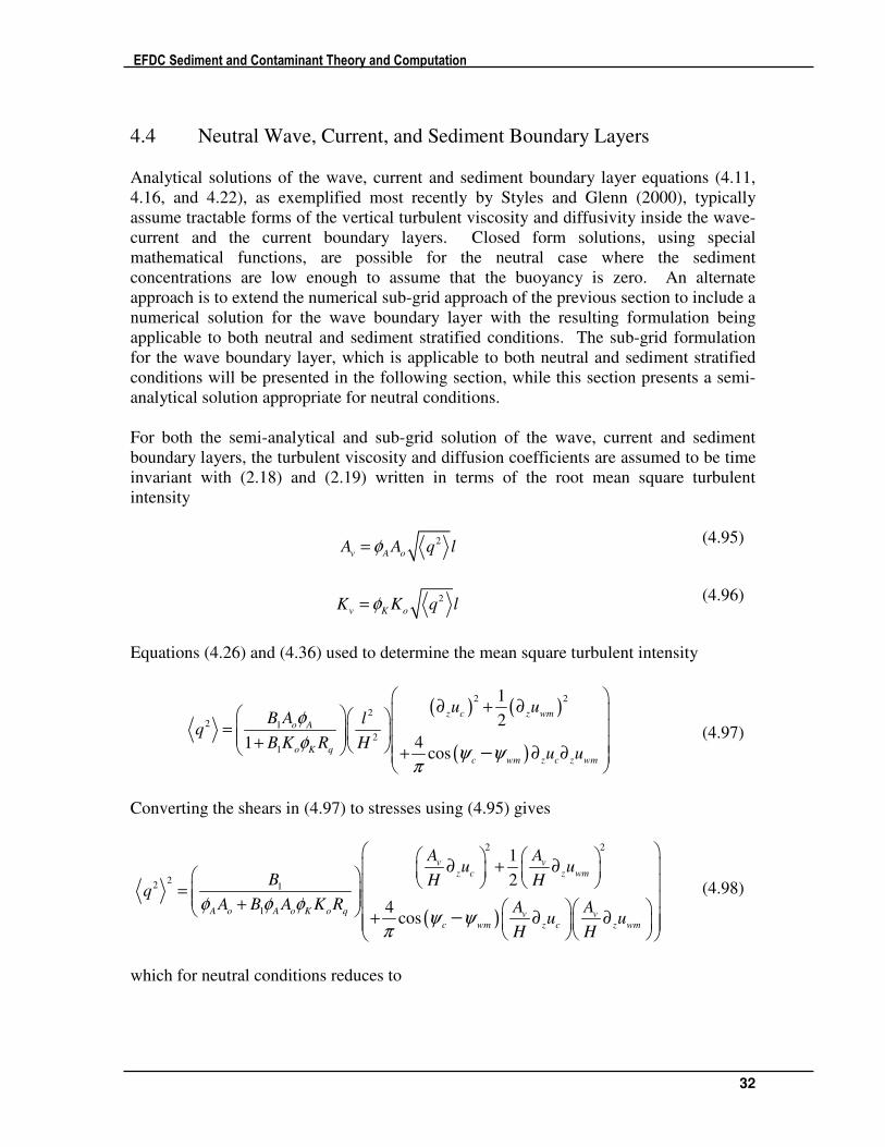
4.4 Neutral Wave, Current, and Sediment Boundary Layers
Analytical solutions of the wave, current and sediment boundary layer equations (4.11,
4.16, and 4.22), as exemplified most recently by Styles and Glenn (2000), typically
assume tractable forms of the vertical turbulent viscosity and diffusivity inside the wave-
current and the current boundary layers. Closed form solutions, using special
mathematical functions, are possible for the neutral case where the sediment
concentrations are low enough to assume that the buoyancy is zero. An alternate
approach is to extend the numerical sub-grid approach of the previous section to include a
numerical solution for the wave boundary layer with the resulting formulation being
applicable to both neutral and sediment stratified conditions. The sub-grid formulation
for the wave boundary layer, which is applicable to both neutral and sediment stratified
conditions will be presented in the following section, while this section presents a semi-
analytical solution appropriate for neutral conditions.
For both the semi-analytical and sub-grid solution of the wave, current and sediment
boundary layers, the turbulent viscosity and diffusion coefficients are assumed to be time
invariant with (2.18) and (2.19) written in terms of the root mean square turbulent
intensity
2
v A oA A q lφ=
(4.95)
2
v K oK K q lφ=
(4.96)
Equations (4.26) and (4.36) used to determine the mean square turbulent intensity
( ) ( )
( )
2 2
22 1
2
1
1
2
41cos
z c z wm
o A
o K qc wm z c z wm
u uB A l
qB K R H
u u
φ
φψ ψ
π
∂ + ∂
= + + ∂ ∂
−
(4.97)
Converting the shears in (4.97) to stresses using (4.95) gives
( )
2 2
22 1
1
1
2
4cos
v v
z c z wm
A o A o K o q v v
c wm z c z wm
A Au u
B H Hq
A B A K R A Au u
H H
φ φ φψ ψ
π
∂ + ∂ = + + ∂ ∂
−
(4.98)
which for neutral conditions reduces to
EFDC Sediment and Contaminant Theory and Computation
33
( )
2 2
22 4/3
1
1
2
4cos
v v
z c z wm
v v
c wm z c z wm
A Au u
H Hq B
A Au u
H Hψ ψ
π
∂ + ∂
= + ∂ ∂
−
(4.99)
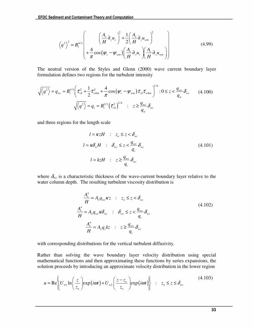
The neutral version of the Styles and Glenn (2000) wave current boundary layer
formulation defines two regions for the turbulent intensity
( )
( )
1/ 4
2 1/3 2 2
1
1/ 42 1/3 2
1
1 4cos : 0
2
:
wcwc cb wbm c wm cb wbm wc
w
wcc cb wc
w
qq q B z
q
qq q B z
q
ψ ψ δπ
δ
τ τ τ τ
τ
= = + + ≤ <
= = ≥
−
(4.100)
and three regions for the length scale
:
:
:
o wc
wcw wc wc
c
wc
wc
c
l zH z z
ql H z
q
ql kzH z
q
κ δ
κδ δ δ
δ
= ≤ <
= ≤ <
= ≥
(4.101)
where δwc is a characteristic thickness of the wave-current boundary layer relative to the
water column depth. The resulting turbulent viscosity distribution is
:
:
:
n
vo wc o wc
n
v wco wc wc wc wc
c
n
v wco c wc
c
AA q z z z
H
A qA q z
H q
A qA q kz z
H q
κ δ
κδ δ δ
δ
= ≤ <
= ≤ <
= ≥
(4.102)
with corresponding distributions for the vertical turbulent diffusivity.
Rather than solving the wave boundary layer velocity distribution using special
mathematical functions and then approximating these functions by series expansions, the
solution proceeds by introducing an approximate velocity distribution in the lower region
( ) ( )1 2Re ln exp exp :ow w o wc
o o
z zzu U i t U i t z z
z zω ω δ
− = + ≤ ≤
(4.103)
EFDC Sediment and Contaminant Theory and Computation
34
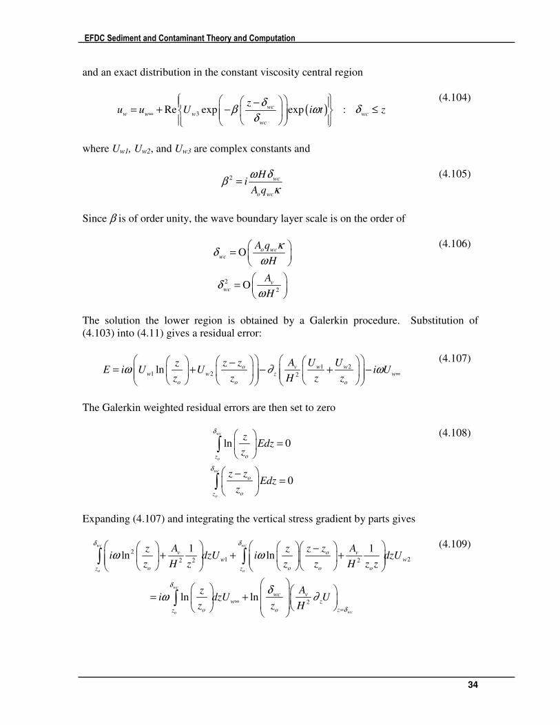
and an exact distribution in the constant viscosity central region
( )3Re exp exp :wcw w w wc
wc
zu u U i t z
δβ ω δ
δ∞
− = + − ≤
(4.104)
where Uw1, Uw2, and Uw3 are complex constants and
2 wc
o wc
Hi
A q
ω δβ
κ=
(4.105)
Since β is of order unity, the wave boundary layer scale is on the order of
2
2
O
O
o wcwc
vwc
A q
H
A
H
κδ
ω
δω
=
=
(4.106)
The solution the lower region is obtained by a Galerkin procedure. Substitution of
(4.103) into (4.11) gives a residual error:
1 21 2 2ln o v w w
w w z w
o o o
z z A U UzE i U U i U
z z H z zω ∂ ω ∞
−= + − + −
(4.107)
The Galerkin weighted residual errors are then set to zero
ln 0
0
wc
o
wc
o
oz
o
oz
zEdz
z
z zEdz
z
δ
δ
=
−=
∫
∫
(4.108)
Expanding (4.107) and integrating the vertical stress gradient by parts gives
2
1 22 2 2
2
1 1ln ln
ln ln
wc wc
o o
wc
wco
v o vw w
o o o oz z
wc vw z
zo oz
A z z Az zi dzU i dzU
z H z z z H z z
Azi dzU U
z z H
δ δ
δ
δ
ω ω
δω ∂∞
=
−+ + +
= +
∫ ∫
∫
(4.109)
EFDC Sediment and Contaminant Theory and Computation
35
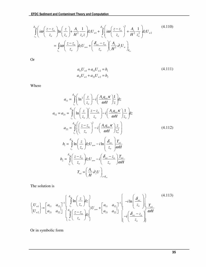
2
1 22 2 2
2
1 1ln
wc wc
o o
wco
o v o vw w
o o o o oz z
o wc o vw z w
o oz
z z A z z Azi dzU i dzU
z z H z z z H z
z z z Ai dzU U
z z H
δ δ
δ
ω ω
δω ∂∞
− − + + +
− − = +
∫ ∫
∫
(4.110)
Or
11 1 12 2 1
21 1 22 2 2
w w
w w
a U a U b
a U a U b
+ =
+ =
(4.111)
Where
2
11
12 21
2
22 2
1
1ln
1ln
ln ln
wc
o
wc
o
wc
o
wc
o
o wc
oz
o o wc
o o oz
o o wc
o oz
wcw
oz
A qza i dz
z H z
z z A qza a i dz
z z H z
z z A q za i
z H z
zb dzU i
z z
δ
δ
δ
δ
κ
ω
κ
ω
κ
ω
δ∞
= −
− = = −
− = −
= −
∫
∫
∫
∫
2
wc
o
wc
wi
o
o wc o wiw
o oz
vwi z
z
T
H
z z z Tb dzU i
z z H
AT U
H
δ
δ
ω
δ
ω
∂
∞
=
− −= −
=
∫
(4.112)
The solution is
1 1
1 11 12 11 12
2 21 22 21 22
ln ln
wc
o
wc
o
wc
oz ow wiw
wo
wc o
ozo
zdz i
z zU a a a a TU
U a a a a Hz z zdz iz z
δ
δ
δ
ωδ
− −
∞
− = +
− − −
∫
∫
(4.113)
Or in symbolic form
EFDC Sediment and Contaminant Theory and Computation
36
1 11 12
2 21 22
wiw w
wiw w
TU A U A
h
TU A U A
h
ω
ω
∞
∞
= +
= +
(4.114)
where the complex stress amplitude Twi at the interface between the lower and central
regions remains to be determined as does the constant, Uw3, in the central region solution.
The two constants, Twi and Uw3, must be determined such that the velocity and its vertical
gradient are continuous at the interface between the two boundary layer regions by the
solution of
( ) ( )
12 22 3
11 21
12 22 11 213
ln
ln
wc wc o wiw
o o
wc wc ow w w
o o
wi
w w
wc o wc wc o
z TA A U
z z h
zU A U A U
z z
TA A A AU U
z h z
δ δ
ω
δ δ
β
δ ω δ δ
∞ ∞ ∞
∞
− + −
−= − −
+ + = − +
(4.115)
The solution provides the interface stress in terms of the inviscid wave velocity amplitude
and in turn allows Uw1 and Uw2 to be expressed in terms of the inviscid wave velocity
amplitude. The maximum wave bed stress can then be determined by
1 2wbm o wc w wA q U Uκτ = + (4.116)
Note that in the absence of currents
1/3
1/ 21
1/ 42wc wbm
Bq τ=
(4.117)
with (4.116) becoming
2
2 2
1 2
221 2
2
2
2
wbm w w bw w
w w
bw
w
U U c U
U Uc
U
κ
κ
τ ∞
∞
= + =
+=
(4.118)
The solution for the current velocity is
EFDC Sediment and Contaminant Theory and Computation
37
lncb
c
o wc o
zu
A q zκ
τ =
(4.119)
in the lower region,
ln 1cb wc
c
o wc wc o
zu
A q z
δ
κ δ
τ = + −
(4.120)
in the central region, and
ln
c
wc
cb wc
c
o wc c e
q
qe wc o
wc c wc
q zu
A q q z
z e q z e
q
κ
δ δ
τ =
=
(4.121)
in the upper region. To enforce the integral constraint, the current profile is integrated
over the three regions to give
( )ln lnwc
o
cb cb wc
wc wc o
o wc o o wc oz
zdz z
A q z A q z
δδ
δ δκ κ
τ τ = − −
∫
(4.122)
2
ln 1
1 11 ln
2 2
wcwc
c
wc
q
q
cb wc
o wc wc o
cb wc wc wc wc
wc
o wc c c c o
zdz
A q z
q q q
A q q q q z
δ
δ
δ
κ δ
δδ
κ
τ
τ
+ −
= − + − +
∫
(4.123)
2
ln
ln 1
ln 1
wcwc
c
m
cb wc
qo wc c e
q
cb wc
o wc c e
cb wc wc wcwc
o wc c e c
q zdz
A q k q z
q mm
A q k q z
q q
A q k q z q
δ
δδ
τ
τ
τ
∆
∆= ∆ −
− −
∫
(4.124)
EFDC Sediment and Contaminant Theory and Computation
38
with the general integral constraint being
( )
( )
1
2
ln
1 11 ln
2 2
ln 1
m
o ck
k
cb wcwc wc o
o wc o
cb wc wc wc wcwc
o wc c c c o
cb wc
o wc c e
cb wc
o wc c
m z u
zA q z
q q q
A q q q q z
q mm
A q q z
q
A q q
δδ δ
κ
δδ
κ
κ
κ
τ
τ
τ
τ
=
∆ −
= − −
+ − + − +
∆+ ∆ −
−
∑
2
ln 1wc wcwc
e c
q
z q
δδ
−
(4.125)
For the thickness of the wave-current layer exceeding the lower hydrodynamic grid layer.
When the wave-current boundary remains inside the bottom layer of the hydrodynamic
grid, (4.125) reduces to
( )
( )
1
3
2 2
ln ln ln
wc c wcwc wc o
c wccbo c c
o wc wc wc wcwc wc
o e c e c
q qz
q qA q u
z q q
z z q z q
δδ δ
κδ δ
δ δ
τ
− + ∆ − −
=
∆ − ∆ + + ∆ −
(4.126)
Introducing (4.100) into (4.126) gives
( )
1 1
22
2
ln 12
cb bc c c
o
bc
wc wc co
e c wc
c u u
zc
q qz
z q q
κ
δ
τ =
∆ −= ∆
∆ − + − +
(4.127)
an expression for the current stress and bottom current friction coefficient.
4.5 Stratified Wave, Current, and Sediment Boundary Layers
Currently under development.
EFDC Sediment and Contaminant Theory and Computation
39
5. Sediment Bed Mass Conservation, Armoring and
Consolidation
The general conservation of mass for bed sediment has the form
( ) ( ) ( ) ( ), , , 1i i i i
t t SB A t PA A t PAkS B k k J k k J k k J∂ δ α δ α δ= − + − − (5.1)
where S is the mass concentration of per total volume of a bed layer k, B is the layer
thickness, JSB is the net sediment mass flux, mass per unit area and unit time, positive
from the bed to the water column, αA is an armoring parameter (1 for armoring, 0
otherwise), and JPA is the parent to armoring layer flux when the top or surface layer of
the bed, kt, acts to simulate armoring. The superscript i denotes the ith sediment size-type
class. The sediment concentration can also be defined by
1
i ii s
FS
ρ
ε=
+
(5.2)
where F is the sediment volume fraction, ρs is the sediment particle density, and ε is the
void ratio. The sediment volume fraction is defined by
1
i ii
k i ii s sk k
S B S BF
ρ ρ
−
= ∑
(5.3)
Assuming that the sediment particles are incompressible (5.1) can be alternately
expressed by
( ) ( ) ( ), , , 11
i i ii
SB PA PAt t A t A ti i i
s s sk
J J JF Bk k k k k k∂ δ α δ α δ
ε ρ ρ ρ
= − + − −
+
(5.4)
Summing (5.4) over the sediment size classes gives
( ) ( ) ( ), , , 11
i i i
SB PA PAt t A t A ti i i
i i ik s s s
J J JBk k k k k k∂ δ α δ α δ
ε ρ ρ ρ
= − + − −
+ ∑ ∑ ∑
(5.5)
The conservation of water volume in a bed layer is given by
EFDC Sediment and Contaminant Theory and Computation
40
( )
( )
( )
: :
1
1
, max ,0 min ,0
,max ,0 min ,0
, 1
t w k w k
k
i ii iSB SB
t kt depi ii is s
i it i iPA PA
A kt kti ii is st
Bq q
J Jk k
k k J J
k k
ε∂
ε
δ ε ερ ρ
δα ε ε
ρ ρδ
− +
−
= −
+
− +
+ + − −
∑ ∑
∑ ∑
(5.6)
Where ε without the i superscript is the bulk void ratio of the bed layer, and ε’s with
superscripts i denote sediment class void ratios required by the mixed material
consolidation formulation to be subsequently discussed. Equations (5.5) and (5.6)
combine to give
( ) ( ) ( )
( ) ( ) ( )
( )
: :
1
, 1 max ,0 1 min ,0
, 1 max ,0 1 min ,0
, 1 1
t k w k w k
i ii iSB SB
t kt depi ii is s
i ii iPA PA
A t kt kti ii is s
A t
B q q
J Jk k
J Jk k
k k
∂
δ ε ερ ρ
α δ ε ερ ρ
α δ ε
− +
−
= −
− + + +
+ + + +
− − +
∑ ∑
∑ ∑
( ) ( )1 max ,0 1 min ,0i i
i iPA PAkt kti i
i is s
J Jε
ρ ρ−
+ +
∑ ∑
(5.7)
The solution procedure for the bed uses a fractional step approach. The first step
involves deposition and resuspension while the second step involves pore water flow and
consolidation.
5. 1 Deposition, Resuspension, and Armoring
The discrete deposition and resuspension step for the sediment class i mass conservation
equation (5.1) is
( ) ( ) ( ) ( ) ( )*
, , , 1n
i i i i i
t SB A t PA A t PAk kS B S B k k J k k J k k Jθδ θα δ θα δ= − + − − (5.8)
Or
( ) ( ) ( )*
, , , 11 1
ni i ii i
SB PA PAt A t A ti i i
s s sk k
J J JF B F Bk k k k k kθδ θα δ θα δ
ε ε ρ ρ ρ
= = − + − −
+ +
(5.9)
The corresponding discrete forms of (5.5), (5.6) and (5.7) are
EFDC Sediment and Contaminant Theory and Computation
41
( ) ( )
( )
*
, ,1 1
, 1
n i i
SB PAt A ti i
i ik k s s
i
PAA t i
i s
J JB Bk k k k
Jk k
θδ θα δε ε ρ ρ
θα δρ
= = − +
+ +
− −
∑ ∑
∑
(5.10)
( )
( ) ( )( )
*
1
, max ,0 min ,01 1
, , 1 max ,0 min ,0
n i ii iSB SB
t kt depi iik k s s
i ii iPA PA
A t t kt kti ii s s
J JB Bk k
J Jk k k k
ε εθδ ε ε
ε ε ρ ρ
θα δ δ ε ερ ρ
−
= − + + +
+ − − +
∑
∑
(5.11)
( ) ( ) ( )
( ) ( ) ( )
( ) ( ) ( )
*
1
1
, 1 max ,0 1 min ,0
, 1 max ,0 1 min ,0
, 1 1 max ,0 1 min ,0
n
k k
i ii iSB SB
t kt depi ii s s
i ii iPA PA
A t kt kti ii s s
i ii iPA PA
A t kt kti i
s s
B B
J Jk k
J Jk k
J Jk k
θδ ε ερ ρ
θα δ ε ερ ρ
θα δ ε ερ ρ
−
−
=
− + + +
+ + + +
− − + + +
∑
∑
i
∑
(5.12)
When the armoring option is inactive, the deposition and resuspension step operates only
on the top layer of the bed with (5.8) solved for the new top layer sediment mass per unit
area
( ) ( )* n
i i i
SBkt ktS B S B Jθ= − (5.13)
using a known sediment depositional or resuspension flux. If the flux in (5.13) is
positive, representing resuspension, it is limited over the time step by
( )( )1min ,n
i i i
SB SBRkt
J J S Bθ −= (5.14)
where the subscript SBR represents the predicted resuspension flux. Following the
solution of (5.13) for each sediment class, equations (5.12) is solved for the new top layer
thickness and (5.10) is solved for the new top layer void ratio.
When the noncohesive sediment armoring option is active, equation (5.8) is applied to the
top two layers of the bed
EFDC Sediment and Contaminant Theory and Computation
42
( ) ( )
( ) ( )
*
*
1 1
ni i i i
SB PAkt kt
ni i i
PAkt kt
S B S B J J
S B S B J
θ θ
θ− −
= − +
= −
(5.15a)
(5.15b)
with the flux limiter (5.14) being applied to (5.15a) for resuspension flux from the top
layer. Two options exist for determining the parent to active layer flux. One option is to
require that the total mass of sediment in the surface, active layer remains constant during
the deposition-resuspension step. The total parent to active layer flux is then given by
(5.10) as
ii
SBPA
i ii is s
JJ
ρ ρ=∑ ∑
(5.16)
The class fluxes can then be assigned by
1 max ,0 min ,0i ii
i iSB SBPAkt kti i i
i is s s
J JJF F
ρ ρ ρ−
= +
∑ ∑
(5.17)
allowing (5.15) to be updated. Equation (5.10) and (5.12) are then solved for the new
thicknesses and void ratios of the parent and active layer. Another option is to require
that the thickness of the active layer to be time invariant during the deposition and
resuspension step. Equation (5.12) reduces to
( ) ( )
( ) ( )
11 max ,0 1 min ,0
1 max ,0 1 min ,0
i ii iPA PAkt kti i
i is s
i ii iSB SBkt depi i
i s s
J J
J J
ε ερ ρ
ε ερ ρ
−
+ + +
= + + +
∑ ∑
∑
(5.18)
The sediment class fluxes can be assigned by
( )( )
( )( )
( ) ( )
1
1
max ,0 min ,01 1
1 max ,0 1 min ,0
i ii
kt ktPASW SWi i i
s kt kt
i ii iSB SB
SW kt depi ii s s
F FJQ Q
J JQ
ρ ε ε
ε ερ ρ
−
−
= ++ +
= + + +
∑
(5.19)
allowing solution of equations (5.15), (5.10), and (5.12).
5. 2 Consolidation of Homogeneous Sediment Beds
This section discusses options for representing consolidation of sediment beds containing
either cohesive sediment or a mixture of noncohesive sediments defined by multiple size
EFDC Sediment and Contaminant Theory and Computation
43
classes. Mixed cohesive and noncohesive bed consolidation is discussed in the
subsequent section. For the second, consolidation half step, the sediment mass per unit
area and the sediment volume per unit area remain constant, with (5.1) and (5.5) giving
( ) ( )1 *n
i i
k kS B S B
+
= (5.20)
1 *
1 1
n
k k
B B
ε ε
+
= + +
(5.21)
The second half step for the water volume conservation equation (5.6) is
( )1 *
: :1 1
n
w k w k
k k
B Bq q
ε εθ
ε ε
+
− +
= + −
+ +
(5.22)
Equations (5.21) and (5.22) can be combined to give
( )1 *
: :
n
k k w k w kB B q qθ+− += + − (5.23)
an equation for the layer thickness, and
( )1
1 *
: :
1n
n
k k w k w k
k
q qB
εε ε θ
+
+
− +
+ = + −
(5.24)
an equation for the void ratio. The EFDC model includes four options for consolidation
and pore water flow.
The first option is a constant porosity bed, with (5.24) giving
: :w k w k GWq q q− += = (5.25)
which indicates that the pore water specific discharge is equal to a specified groundwater
specific discharge at the bottom of the lowest bed layer. The second option is a simple
consolidation model based on relaxation of the vertical void ratio profile to a specified
profile given by
( ) ( )( )expm o m c ot tε ε ε ε α= + − − − (5.26)
where αc is a consolidation rate coefficient, and εm is an ultimate minimum void ratio,
which can be dependent on the vertical position in the bed. Evaluating (5.26) at two
successive time levels gives
( ) ( )( )expn
m o m c on tε ε ε ε α θ− = − − − (5.27)
EFDC Sediment and Contaminant Theory and Computation
44
( ) ( )( )1 expn
m o m c on tε ε ε ε α θ θ+ − = − − + − (5.28)
Taking their ratio gives
( )1
*exp
n
mc
m
ε εα θ
ε ε
+ −= −
−
(5.29)
or
( ) ( )1 * expn
k m k m cε ε ε ε α θ+ = + − − (5.30)
Using the new void ratio given by (5.30), the new bed layer thickness is updated by
(5.21). The pore water specific discharges are then given by recursively solving (5.23)
( )1 1 *
: :
n
w k w k k kq q B Bθ − +
+ −= − − (5.31)
From k = 1, kt using
:1w GWq q− = (5.32)
The third option for consolidation and pore water flow is based on finite strain
consolidation theory. Use of this option requires the bed layers to be composed of either
cohesive or noncohesive sediment, such that a single set of constitutive relationships are
used over the entire thickness of the bed. The specific discharges in (5.23) or (5,24) are
determined using the Darcy equation
z
w
Kq u
g∂
ρ= −
(5.33)
where K is the hydraulic conductivity and u is the excess pore pressure defined as the
difference between the total pore pressure, ut, and the hydrostatic pressure, uh.
t hu u u= − (5.34)
The total pore pressure is defined as the difference between the total stress σ and
effective stress σe.
t eu σ σ= − (5.35)
The total stress and hydrostatic pressure are given by
EFDC Sediment and Contaminant Theory and Computation
45
( )1
1 1
bz
i i
b w s
iz
p g F dzε
σ ρ ρε ε
= + +
+ + ∑∫
(5.36)
( )h b w bu p g z zρ= + − (5.37)
where pb is the water column pressure at the bed surface zb. Solving for the excess pore
pressure using (5.34) through (5.37) gives
11
1
bz
sw e
wz
u g dzρ
ρ σε ρ
= − − +
∫ (5.38)
where
( )i i
s s
i
Fρ ρ=∑ (5.39)
is the average sediment density. The specific discharge (5.33), can alternately be
expressed in terms of the effective stress
11
sz e
w w
K Kq
g
ρ∂ σ
ρ ρ ε
= + −
+
(5.40)
or the void ratio
11
e sz
w w
K Kq
g
σ ρ∂ ε
ρ ε ρ ε
∂ = + −
∂ +
(5.41)
where dε/dσc is a coefficient of compressibility. For consistency with the Lagrangian
representation of sediment mass conservation, a new vertical coordinate ζ, defined by
1
1
d
dz
ζ
ε=
+
(5.42)
is introduced, with (5.40) and (5.41) becoming
11 1
e sw
w w
K Kq
gζ
σ ρ∂
ε ρ ρ ε
= + −
+ +
(5.43)
and
EFDC Sediment and Contaminant Theory and Computation
46
11 1
sw
w
K Kq ζ
ρλ ∂ ε
ε ρ ε
= − + −
+ +
(5.44)
where λ is a length scale
1 e
wg
∂σλ
ρ ∂ε= −
(5.45)
The consistency of (5.43) and (5.44) at bed layer interfaces also requires consideration.
The finite difference form of (5.33) in the transformed coordinate, defined by (5.42), at
an interface between bed layers can be written as
2
1
i k
kw k
u uKq
gρ ε
− = −
+ ∆
(5.46)
below the interface and
1
1 1
2
1
k i
kw k
u uKq
gρ ε+
+ +
− = −
+ ∆
(5.47)
above the interface, where
( )1k k kBε∆ = + (5.48)
is the transformed coordinate thickness of the bed layer. Solving (5.47) for the interface
excess pore pressure and inserting the results into (5.46) gives
( )( )
1
1/ 2 1
2
1
k k
k w k k
u uKq
gε ρ+
+ +
− = −
+ ∆ + ∆
(5.49)
where
( )1 1
1/ 2 1
1 1 1k k k k
k k kK K K
ε ε ε+ +
+ +
+ + + ∆ + ∆ = ∆ + ∆
(5.50)
defines the hydraulic conductivity at the bed layer interface between layers k and k+1.
The discrete from of (5.38) in the transformed coordinate is
EFDC Sediment and Contaminant Theory and Computation
47
1 1
1
1 12 2
s s
w w w wk k k k
e e
w wk k
u u
g g
g g
ρ ρ
ρ ρ ρ ρ
σ σ
ρ ρ
+ +
+
∆ ∆− = − − + −
− +
(5.51)
which after introduction into (5.49) gives
( )1/ 2 1 1
1/ 2 1/ 2
2
1
11
e e
k k k w wk k
s
k w k
Kq
g g
K
σ σ
ε ρ ρ
ρ
ε ρ
+ + +
+ +
= − + ∆ + ∆
+ −
+
(5.52)
where
( ) 1
11/ 2 1
11 1 1s s s
k k
w k k w wk k k
ρ ρ ρ
ρ ρ ρ+
++ +
− = ∆ − + ∆ − ∆ + ∆
(5.53)
In terms of the void ratio, (5.52) is
( )( )1/ 2
1
1/ 2 1/ 21 1/ 2
21
1 1
k sk k
k kk k w k
K Kq
λ ρε ε
ε ε ρ+
+
+ ++ +
= − − + −
+ ∆ + ∆ +
(5.54)
where
, 1 ,
1/ 2
1
1 e k e k
k
w k kg
σ σλ
ρ ε ε+
+
+
− = −
−
(5.55)
The effective stress and hydraulic conductivity are functions of the void ratio. For
cohesive material
exp
exp
e o
eo
e eo o
σ
σ σ
σ ε ε
σ ε
∂σ σ ε ε
∂ε ε ε
−= −
−= − −
(5.56)
exp o
o K
K
K
ε ε
ε
−=
(5.57)
EFDC Sediment and Contaminant Theory and Computation
48
are the simplest functional relationships consistent with observational data. Figures 5.1
through 5.4, based on data presented in Cargill (1985) and Palermo et al. (1998) confirm
these choices. However, they show essentially two regions of behavior, below and above
a void ratio of approximately 6. For noncohesive material the linear relationships
1e o
eo
e eo
σ
σ
σ ε ε
σ ε
∂σ σ
∂ε ε
−= −
= −
(5.58)
1 o
o K
K
K
ε ε
ε
−= +
(5.59)
are appropriate.
Given the unique dependence of the specific discharge on the void ratio, the void ratio
form of the consolidation step, (5.24) is selected for the solution, with the thickness of the
bed layers then determined by (5.23). The specific discharges at the top and bottom of
layer k, follow from (5.54) and are given by
( )
( )
: 1
1
: 1
1
21
1 1
21
1 1
k sw k k k
k kk k w k
k sw k k k
k kk k w k
K Kq
K Kq
λ ρε ε
ε ρ ε
λ ρε ε
ε ρ ε
++ +
+ ++ +
−− −
− −− −
= − − + −
∆ + ∆ + +
= − − + −
∆ + ∆ + +
(5.60)
For the bottom layer of the bed,
:1w gwiq q− = (5.61)
where qgwi is a known specific discharge due to groundwater interaction.
For the top layer of the bed, two alternate formulations are possible. The first
formulation assumes that the void ratio at the water column-sediment bed interface is
specified by εdep, with (5.60a) modified to
( ):
21
1 1
kt sw kt dep k
kt ktkt w kt
K Kq
λ ρε ε
ε ρ ε+
+
+ ++
= − − + −
∆ + +
(5.62)
The second formulation assumes that the excess pore pressure, u, at the water column-
sediment bed interface is zero with (5.46) giving
EFDC Sediment and Contaminant Theory and Computation
49
:
2
1w kt
Kt Kt w Kt
K uq
gε ρ+
=
+ ∆
(5.63)
Using (5.38) the excess pore pressure at the midpoint of the top layer is
12
s e
w w w
u
g g
ρ σ
ρ ρ ρ
∆= − −
(5.64)
which combines with (5.63) to give
:
21
1 1
e sw kt
Kt KtKt w w Kt
K Kq
g
σ ρ
ε ρ ε ρ+
= − + −
+ ∆ +
(5.65)
Equation (5.65) can be expressed in terms of the void ratio at the new time level n+1 by
expanding the effective stress at time level n+1 in a Taylor series
( ) ( )1 1 *nn n n
e e eεσ σ σ ε ε+ += + ∂ − (5.66)
Substituting (5.61) into (5.65) gives
* 1
:
* *
21
1 1
2
1
n sw kt
Kt KtKt w Kt
n
e
Kt Kt w Kt
K Kq
K
g
ρλ ε
ε ε ρ
σλ ε
ε ρ
++
= + −
+ ∆ +
− +
+ ∆
(5.67)
The numerical values of the various parameters in the expressions for the specific
discharge indicate that an implicit solution of (5.24) is necessary. This is done in two
stages with an intermediate void ratio, denoted by **, determined by substituting the
internal specific discharges, written as
( )
( )
* * ***
: 1
1
* * ***
: 1
1
21
1 1
21
1 1
k sw k k k
k kk k w k
k sw k k k
k kk k w k
K Kq
K Kq
λ ρε ε
ε ρ ε
λ ρε ε
ε ρ ε
++ +
− ++ +
−− −
− −− −
= − − + −
∆ + ∆ + +
= − − + −
∆ + ∆ + +
(5.68)
and one of the surface specific discharges corresponding to (5.62)
( )** * *
**
:
21
1 1
sw kt dep k
kt kt ktw kt
K Kq
ρλε ε
ε ρ ε+
+ +
= − − + −
∆ + +
(5.69)
EFDC Sediment and Contaminant Theory and Computation
50
or (5.67)
* * *
**
:
**
21
1 1
2
1
sw kt
kt kt kt w
e
kt kt w kt
K Kq
K
g
ρλε
ε ε ρ
σλε
ε ρ
+
+ +
+
= + −
+ ∆ +
− +
+ ∆
(5.70)
into
( )**
** *
: :
1
2k k w k w k
k
q qB
θ εε ε − +
+ = + −
(5.71)
and solving the resulting tri-diagonal system of equations. The specific discharges are
then exactly calculated using (5.68) and (5.69) or (5.70). The new time level thickness of
the layers is determined by (5.23) with the void ratios determined from (5.24). The
linearized form of this scheme is unconditionally stable.
5. 3 Consolidation of Mixed Cohesive and Noncohesive Sediment Beds
This section presents a methodology for representing consolidation of sediment beds
containing both cohesive and noncohesive sediments. The methodology allows for both
cohesive and noncohesive sediment in any bed layer and is based on the following
assumptions. First, it is assumed that during the consolidation step, a fraction of the bed
pore water volume per unit horizontal area is associated with each sediment type or
( )1
wc wn
BB
εψ ψ
ε
= +
+
(5.72)
where the subscripts wc and wn denote water associated with cohesive and noncohesive
sediment, respectively. Likewise the volume of sediment per unit horizontal area can be
fractionally partitioned between cohesive and noncohesive
( )1
sc sn
BBψ ψ
ε
= +
+
(5.73)
Following the Lagrangian formulation of the previous section, the total volume of
sediment and the fractional sediment volume in a bed layer remain constant during a
consolidation step.
( ) ( ) 0t sc t snB Bψ ψ∂ = ∂ = (5.74)
Fractional void ratios can also be defined
EFDC Sediment and Contaminant Theory and Computation
51
wcc
sc
ψε
ψ=
(5.75)
wnn
sn
ψε
ψ=
(5.76)
and using (5.72) and (5.73), the void ratio of the mixture is
sc c sn n
sc sn
ψ ε ψ εε
ψ ψ
+=
+
(5.77)
which is the sediment volume weighted average of the void ratios of the two sediment
types.
The second assumption is that during the consolidation time step, the fraction of water
associated with noncohesive sediment remains constant, as does the fractional void ratio.
This is equivalent to the assuming that the portion of the bed layer associated with
noncohesive sediment is incompressible, and that the pore water associated the
noncohesive sediment is specified by εn.
Consistent with the preceding assumptions, the thickness of the bed layer can be divided
into cohesive and noncohesive fractions, Bc and Bn, respectively.
( ) ( )
( ) ( )
1
1
c wc sc c sc
n wn sn n sn
B B B
B B B
ψ ψ ε ψ
ψ ψ ε ψ
= + = +
= + = +
(5.78)
The hydraulic conductivity of the layer can be expressed by
( )c n
c n
c n
B BK
B B
K K
+=
+
(5.79)
which is equivalent to an infinite number of alternating infinitesimal cohesive and
noncohesive sublayers of proportional thickness comprising the mixed bed layer.
Equation (5.79) can be written as
( ) ( ) ( )1
1 1 1c n
sc sn
c n
K
f fK K
ε ε ε=
+ + + +
(5.80)
where
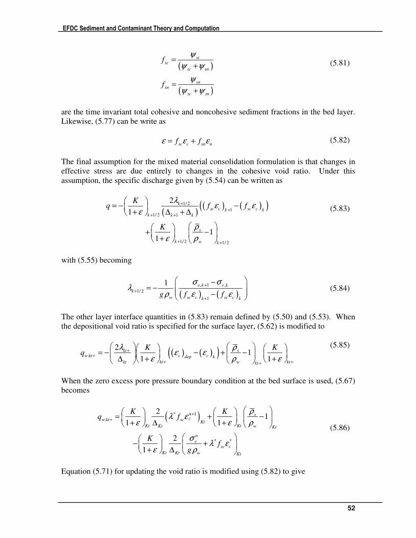
EFDC Sediment and Contaminant Theory and Computation
52
( )
( )
scsc
sc sn
snsn
sc sn
f
f
ψ
ψ ψ
ψ
ψ ψ
=+
=+
(5.81)
are the time invariant total cohesive and noncohesive sediment fractions in the bed layer.
Likewise, (5.77) can be write as
sc c sn nf fε ε ε= + (5.82)
The final assumption for the mixed material consolidation formulation is that changes in
effective stress are due entirely to changes in the cohesive void ratio. Under this
assumption, the specific discharge given by (5.54) can be written as
( )( ) ( )( )1/ 2
11/ 2 1
1/ 2 1/ 2
2
1
11
ksc c sc ck k
k k k
s
k w k
Kq f f
K
λε ε
ε
ρ
ε ρ
+
++ +
+ +
= − −
+ ∆ + ∆
+ −
+
(5.83)
with (5.55) becoming
( ) ( ), 1 ,
1/ 2
1
1 e k e k
k
w sc c sc ck kg f f
σ σλ
ρ ε ε+
+
+
−= − −
(5.84)
The other layer interface quantities in (5.83) remain defined by (5.50) and (5.53). When
the depositional void ratio is specified for the surface layer, (5.62) is modified to
( ) ( )( ):
21
1 1
kt sw kt c cdep k
kt ktkt w kt
K Kq
λ ρε ε
ε ρ ε+
+
+ ++
= − − + −
∆ + +
(5.85)
When the zero excess pore pressure boundary condition at the bed surface is used, (5.67)
becomes
( )* 1
:
* *
21
1 1
2
1
C
n sw kt sc
KtKt KtKt w Kt
n
esc c
Kt Kt w Kt
K Kq f
Kf
g
ρλ ε
ε ε ρ
σλ ε
ε ρ
++
= + −
+ ∆ +
− +
+ ∆
(5.86)
Equation (5.71) for updating the void ratio is modified using (5.82) to give
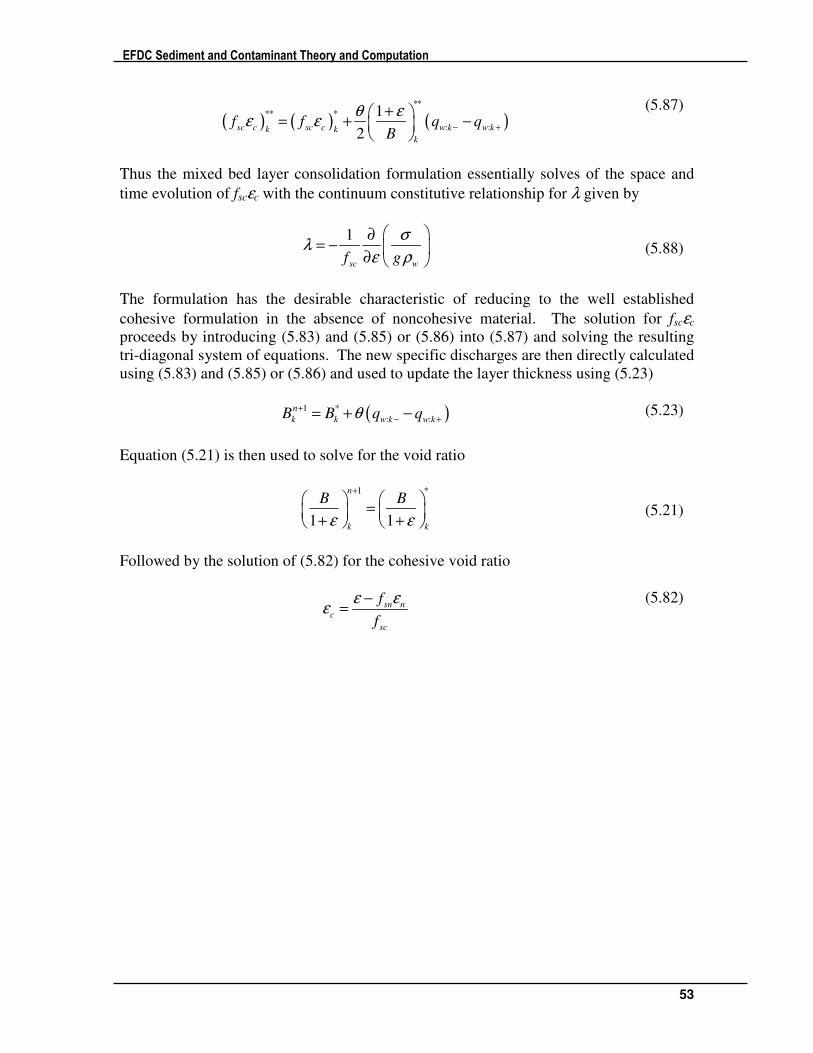
EFDC Sediment and Contaminant Theory and Computation
53
( ) ( ) ( )**
** *
: :
1
2sc c sc c w k w kk k
k
f f q qB
θ εε ε − +
+ = + −
(5.87)
Thus the mixed bed layer consolidation formulation essentially solves of the space and
time evolution of fscεc with the continuum constitutive relationship for λ given by
1
sc wf g
σλ
ε ρ
∂= −
∂
(5.88)
The formulation has the desirable characteristic of reducing to the well established
cohesive formulation in the absence of noncohesive material. The solution for fscεc
proceeds by introducing (5.83) and (5.85) or (5.86) into (5.87) and solving the resulting
tri-diagonal system of equations. The new specific discharges are then directly calculated
using (5.83) and (5.85) or (5.86) and used to update the layer thickness using (5.23)
( )1 *
: :
n
k k w k w kB B q qθ+− += + − (5.23)
Equation (5.21) is then used to solve for the void ratio
1 *
1 1
n
k k
B B
ε ε
+
= + +
(5.21)
Followed by the solution of (5.82) for the cohesive void ratio
sn nc
sc
f
f
ε εε
−=
(5.82)
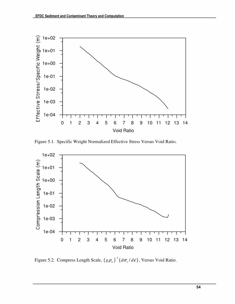
EFDC Sediment and Contaminant Theory and Computation
54
Figure 5.1. Specific Weight Normalized Effective Stress Versus Void Ratio.
Figure 5.2. Compress Length Scale, ( ) ( )1
/w e
g d dρ σ ε−
, Versus Void Ratio.
0 1 2 3 4 5 6 7 8 9 10 11 12 13 14
1e-04
1e-03
1e-02
1e-01
1e+00
1e+01
1e+02
Void Ratio
0 1 2 3 4 5 6 7 8 9 10 11 12 13 14
1e-04
1e-03
1e-02
1e-01
1e+00
1e+01
1e+02
Void Ratio
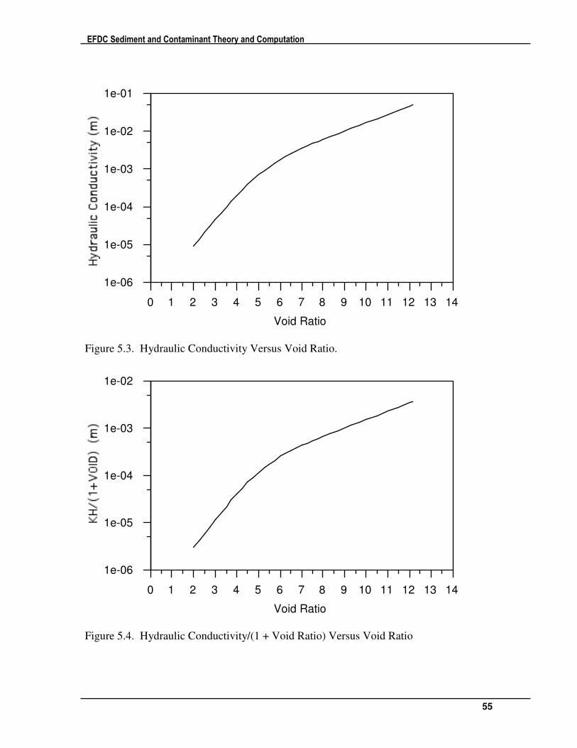
EFDC Sediment and Contaminant Theory and Computation
55
Figure 5.3. Hydraulic Conductivity Versus Void Ratio.
Figure 5.4. Hydraulic Conductivity/(1 + Void Ratio) Versus Void Ratio
0 1 2 3 4 5 6 7 8 9 10 11 12 13 14
1e-06
1e-05
1e-04
1e-03
1e-02
1e-01
Void Ratio
0 1 2 3 4 5 6 7 8 9 10 11 12 13 14
1e-06
1e-05
1e-04
1e-03
1e-02
Void Ratio
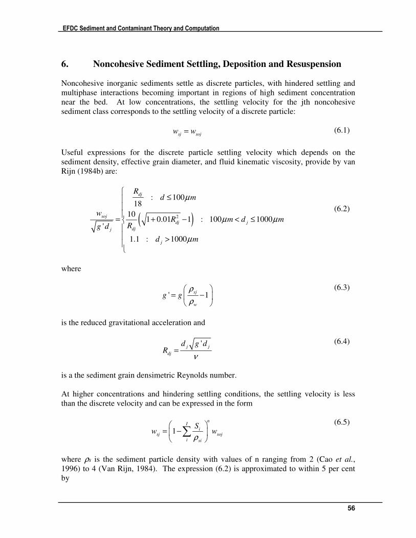
EFDC Sediment and Contaminant Theory and Computation
56
6. Noncohesive Sediment Settling, Deposition and Resuspension
Noncohesive inorganic sediments settle as discrete particles, with hindered settling and
multiphase interactions becoming important in regions of high sediment concentration
near the bed. At low concentrations, the settling velocity for the jth noncohesive
sediment class corresponds to the settling velocity of a discrete particle:
sj sojw w= (6.1)
Useful expressions for the discrete particle settling velocity which depends on the
sediment density, effective grain diameter, and fluid kinematic viscosity, provide by van
Rijn (1984b) are:
( )2
: 10018
101 0.01 1 : 100 1000
'
1.1 : 1000
dj
soj
dj j
djj
j
Rd m
wR m d m
Rg d
d m
µ
µ µ
µ
≤
= + − < ≤ >
(6.2)
where
' 1sj
w
g gρ
ρ
= −
(6.3)
is the reduced gravitational acceleration and
'j j
dj
d g dR
ν=
(6.4)
is a the sediment grain densimetric Reynolds number.
At higher concentrations and hindering settling conditions, the settling velocity is less
than the discrete velocity and can be expressed in the form
1
nI
isj soj
i si
Sw w
ρ
= − ∑
(6.5)
where ρs is the sediment particle density with values of n ranging from 2 (Cao et al.,
1996) to 4 (Van Rijn, 1984). The expression (6.2) is approximated to within 5 per cent
by
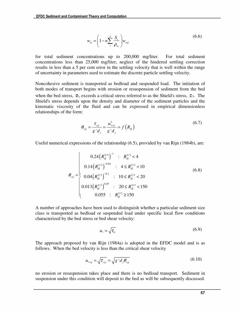
EFDC Sediment and Contaminant Theory and Computation
57
1I
isj soj
i si
Sw n w
ρ
= −
∑ (6.6)
for total sediment concentrations up to 200,000 mg/liter. For total sediment
concentrations less than 25,000 mg/liter, neglect of the hindered settling correction
results in less than a 5 per cent error in the settling velocity that is well within the range
of uncertainty in parameters used to estimate the discrete particle settling velocity.
Noncohesive sediment is transported as bedload and suspended load. The initiation of
both modes of transport begins with erosion or resuspension of sediment from the bed
when the bed stress, τb, exceeds a critical stress referred to as the Shield's stress, τcs. The
Shield's stress depends upon the density and diameter of the sediment particles and the
kinematic viscosity of the fluid and can be expressed in empirical dimensionless
relationships of the form:
( )2
*
' '
csj csj
csj dj
j j
uf R
g d g d
τθ = = =
(6.7)
Useful numerical expressions of the relationship (6.5), provided by van Rijn (1984b), are:
( )
( )
( )
( )
12 /3 2 /3
0.642 /3 2 /3
0.12/3 2/3
0.292/3 2/3
2/3
0.24 : 4
0.14 : 4 10
0.04 : 10 20
0.013 : 20 150
0.055 : 150
dj dj
dj dj
csjdj dj
dj dj
dj
R R
R R
R R
R R
R
θ
−
−
−
<
≤ <
= ≤ < ≤ < ≥
(6.8)
A number of approaches have been used to distinguish whether a particular sediment size
class is transported as bedload or suspended load under specific local flow conditions
characterized by the bed stress or bed shear velocity:
* bu τ= (6.9)
The approach proposed by van Rijn (1984a) is adopted in the EFDC model and is as
follows. When the bed velocity is less than the critical shear velocity
* 'csj csj j csj
u g d θτ= = (6.10)
no erosion or resuspension takes place and there is no bedload transport. Sediment in
suspension under this condition will deposit to the bed as will be subsequently discussed.
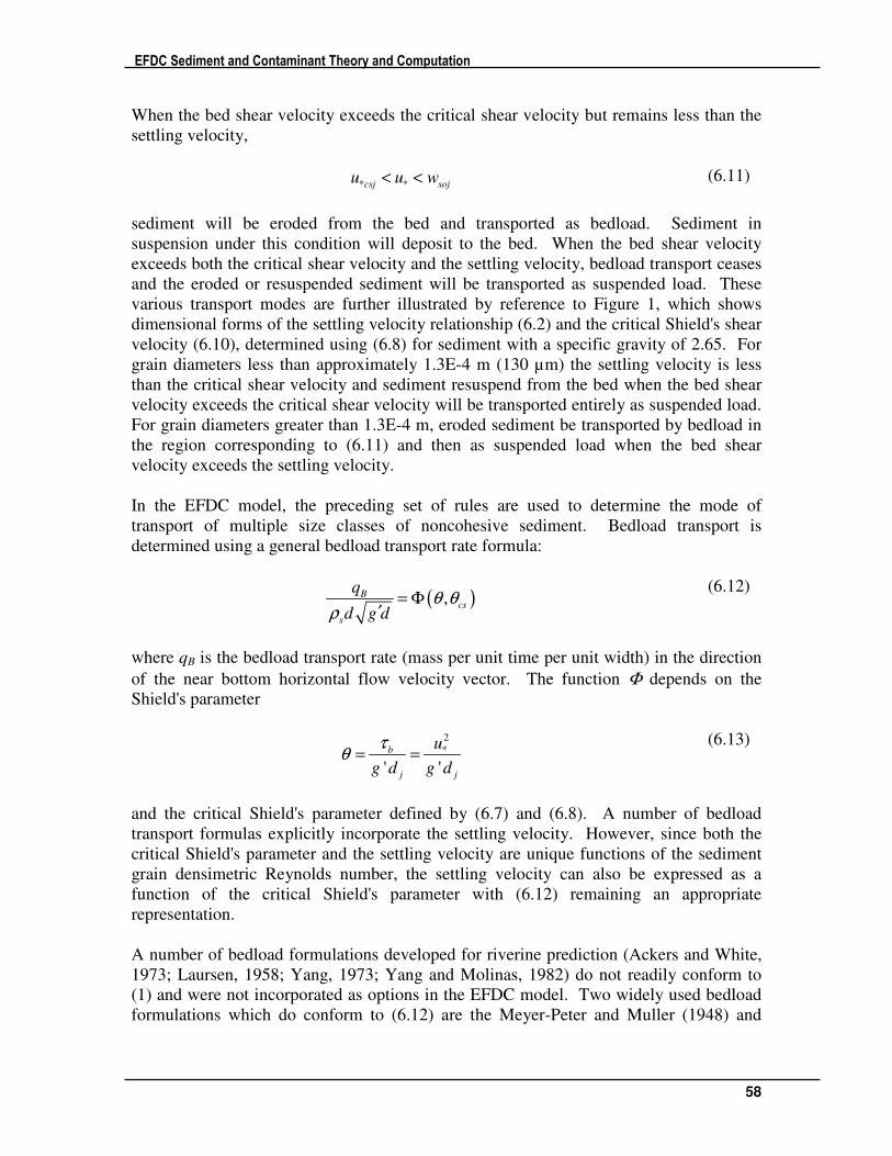
EFDC Sediment and Contaminant Theory and Computation
58
When the bed shear velocity exceeds the critical shear velocity but remains less than the
settling velocity,
* *csj soju u w< < (6.11)
sediment will be eroded from the bed and transported as bedload. Sediment in
suspension under this condition will deposit to the bed. When the bed shear velocity
exceeds both the critical shear velocity and the settling velocity, bedload transport ceases
and the eroded or resuspended sediment will be transported as suspended load. These
various transport modes are further illustrated by reference to Figure 1, which shows
dimensional forms of the settling velocity relationship (6.2) and the critical Shield's shear
velocity (6.10), determined using (6.8) for sediment with a specific gravity of 2.65. For
grain diameters less than approximately 1.3E-4 m (130 µm) the settling velocity is less
than the critical shear velocity and sediment resuspend from the bed when the bed shear
velocity exceeds the critical shear velocity will be transported entirely as suspended load.
For grain diameters greater than 1.3E-4 m, eroded sediment be transported by bedload in
the region corresponding to (6.11) and then as suspended load when the bed shear
velocity exceeds the settling velocity.
In the EFDC model, the preceding set of rules are used to determine the mode of
transport of multiple size classes of noncohesive sediment. Bedload transport is
determined using a general bedload transport rate formula:
( ),Bcs
s
q
d g dθ θ
ρ= Φ
′
(6.12)
where qB is the bedload transport rate (mass per unit time per unit width) in the direction
of the near bottom horizontal flow velocity vector. The function Φ depends on the
Shield's parameter
2
*
' '
b
j j
u
g d g d
τθ = =
(6.13)
and the critical Shield's parameter defined by (6.7) and (6.8). A number of bedload
transport formulas explicitly incorporate the settling velocity. However, since both the
critical Shield's parameter and the settling velocity are unique functions of the sediment
grain densimetric Reynolds number, the settling velocity can also be expressed as a
function of the critical Shield's parameter with (6.12) remaining an appropriate
representation.
A number of bedload formulations developed for riverine prediction (Ackers and White,
1973; Laursen, 1958; Yang, 1973; Yang and Molinas, 1982) do not readily conform to
(1) and were not incorporated as options in the EFDC model. Two widely used bedload
formulations which do conform to (6.12) are the Meyer-Peter and Muller (1948) and
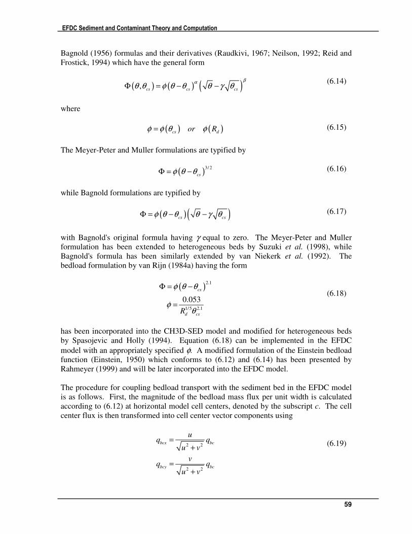
EFDC Sediment and Contaminant Theory and Computation
59
Bagnold (1956) formulas and their derivatives (Raudkivi, 1967; Neilson, 1992; Reid and
Frostick, 1994) which have the general form
( ) ( ) ( ),cs cs cs
βαθ θ φ θ θ θ γ θΦ = − −
(6.14)
where
( ) ( )cs dor Rφ φ θ φ= (6.15)
The Meyer-Peter and Muller formulations are typified by
( )3/ 2
csφ θ θΦ = − (6.16)
while Bagnold formulations are typified by
( )( )cs csφ θ θ θ γ θΦ = − − (6.17)
with Bagnold's original formula having γ equal to zero. The Meyer-Peter and Muller
formulation has been extended to heterogeneous beds by Suzuki et al. (1998), while
Bagnold's formula has been similarly extended by van Niekerk et al. (1992). The
bedload formulation by van Rijn (1984a) having the form
( )2.1
1/5 2.1
0.053
cs
d csR
φ θ θ
φθ
Φ = −
=
(6.18)
has been incorporated into the CH3D-SED model and modified for heterogeneous beds
by Spasojevic and Holly (1994). Equation (6.18) can be implemented in the EFDC
model with an appropriately specified φ. A modified formulation of the Einstein bedload
function (Einstein, 1950) which conforms to (6.12) and (6.14) has been presented by
Rahmeyer (1999) and will be later incorporated into the EFDC model.
The procedure for coupling bedload transport with the sediment bed in the EFDC model
is as follows. First, the magnitude of the bedload mass flux per unit width is calculated
according to (6.12) at horizontal model cell centers, denoted by the subscript c. The cell
center flux is then transformed into cell center vector components using
2 2
2 2
bcx bc
bcy bc
uq q
u v
vq q
u v
=+
=+
(6.19)
EFDC Sediment and Contaminant Theory and Computation
60
where u and v are the cell center horizontal velocities near the bed. Cell face mass fluxes
are determined by down wind projection of the cell center fluxes
( )
( )bfx bcx upwind
bfy bcy upwind
q q
q q
=
=
(6.20)
where the subscript upwind denotes the cell center upwind of the x normal and y normal
cell faces. The net removal or accumulation rate of sediment material from the deposited
bed underlying a water cell is then given by:
( ) ( ) ( ) ( )x y b y bfx y bfx x bfy x bfye w n sm m J m q m q m q m q= − + − (6.21)
where Jb is the net removal rate (gm/m2-sec) from the bed, mx and my are x and y
dimensions of the cell, and the compass direction subscripts define the four cell faces.
The implementation of (6.19) through (6.21) in the EFDC code includes logic to limit the
out fluxes (6.20) over a time step, such that the time integrated mass flux from the bed
does not exceed bed sediment available for erosion or resuspension.
Under conditions when the bed shear velocity exceeds the settling velocity and critical
Shield's shear velocity, noncohesive sediment will be resuspended and transported as
suspended load. When the bed shear velocity falls below both the settling velocity and
the critical Shield's shear velocity, suspended sediment will deposit to the bed. A
consistent formulation of these processes can be developed using the concept of a near
bed equilibrium sediment concentration. Under steady, uniform flow and sediment
loading conditions, an equilibrium distribution of sediment in the water column tends to
be established, with the resuspension and deposition fluxes canceling each other. Using a
number of simplifying assumptions, the equilibrium sediment concentration distribution
in the water column can be expressed analytically in terms of the near bed reference or
equilibrium concentration, the settling velocity and the vertical turbulent diffusivity. For
unsteady or spatially varying flow conditions, the water column sediment concentration
distribution varies in space and time in response to sediment load variations, changes in
hydrodynamic transport, and associated nonzero fluxes across the water column-sediment
bed interface. An increase or decrease in the bed stress and the intensity of vertical
turbulent mixing will result in net erosion or deposition, respectively, at a particular
location or time.
To illustrate how an appropriate suspended noncohesive sediment bed flux boundary
condition can be established, consider the approximation to the sediment transport
equation (3.1) for nearly uniform horizontal conditions
( ) vt z z s
KHS S w S
H∂ ∂ ∂
= +
(6.22)
Integrating (6.22) over the depth of the bottom hydrodynamic model layer gives
EFDC Sediment and Contaminant Theory and Computation
61
( ) 0tHS J J∂ ∆∆ = − (6.23)
where the over bar denotes the mean over the dimensionless layer thickness, ∆.
Subtracting (6.23) from (6.22) gives
( ) 0vt z z s
K J JHS S w S
H∂ ∂ ∂ ∆−
′ = + − ∆
(6.24)
Assuming that the rate of change of the deviation of the sediment concentration from the
mean is small
( ) ( )t tHS HS∂ ∂′ << (6.25)
allows (6.24) to be approximated by
0vz z s
K J JS w S
H∂ ∂ ∆−
+ = ∆
(6.26)
Integrating (6.26) once gives
( )0 0v
z s
K zS w S J J J
H∂ ∆+ = − −
∆
(6.27)
Very near the bed, (6.27) can be approximated by
0v
z s
KS w S J
H∂ + = −
(6.28)
Neglecting stratification effects and using the results of Chapter 4, the near bed
diffusivity is approximately
*v
o
K lK q u z
H Hκ= ≅
(6.29)
Introducing (6.29) into (6.28) gives
oz
s
JR RS S
z z w∂ + = −
(6.30)
where
EFDC Sediment and Contaminant Theory and Computation
62
*
sw
Ru κ
= (6.31)
is the Rouse parameter. The solution of (6.30) is
o
R
s
J CS
w z= − +
(6.32)
The constant of integration is evaluated using
: 0eq eq o
S S z z and J= = = (6.33)
which sets the near bed sediment concentration to an equilibrium value, defined just
above the bed under no net flux condition. Using (6.33), equation (6.32) becomes
R
eq oeq
s
z JS S
z w
= −
(6.34)
For non-equilibrium conditions, the net flux is given by evaluating (6.34) at the
equilibrium level
( )o s eq neJ w S S= − (6.35)
where Sne is the actual concentration at the reference equilibrium level. Equation (6.35)
clearly indicates that when the near bed sediment concentration is less than the
equilibrium value a net flux from the bed into the water column occurs. Likewise when
the concentration exceeds equilibrium, a net flux to the bed occurs. For this case when
Sne is greater than Seq
1eq
o s ne
ne
SJ w S
S
= − −
(6.35b)
and the term inside the ( ) can be considered as the deposition factor which does not
exceed unity.
For the relationship (6.35) to be useful in a numerical model, the bed flux must be
expressed in terms of the model layer mean concentration. For a three-dimensional
application, (6.34) can be integrated over the bottom model layer to give
( )o s eqJ w S S= − (6.36)
where
EFDC Sediment and Contaminant Theory and Computation
63
( )( )
( )( )( ) ( )
1
1
11
1
ln: 1
1
1: 1
1 1
eq
eq eq
eq
R
eq
eq eq
eq
zS S R
z
z
S S RR z
−
−
−−
−
∆= =
∆ −
∆ −= ≠
− ∆ −
(6.37)
defines an equivalent layer mean equilibrium concentration in terms of the near bed
equilibrium concentration. The corresponding quantities in the numerical solution
bottom boundary condition (3.6) are
r r s eq
d s s
w S w S
P w w
=
=
(6.38)
If the dimensionless equilibrium elevation, zeq exceeds the dimensionless layer thickness,
(6.19) can be modified to
( )( )
( )( )( ) ( )
1
1
11
1
ln: 1
1
1: 1
1 1
eq
eq eq
eq
R
eq
eq eq
eq
M zS S R
M z
M z
S S RR M z
−
−
−−
−
∆= =
∆ −
∆ −= ≠
− ∆ −
(6.39)
where the over bars in (6.36) and (6.38) implying an average of the first M layers above
the bed.
For two-dimensional, depth averaged model application, a number of additional
considerations are necessary. For depth average modeling, the equivalent of (6.27) is
( )1vz s o
KS w S J z
H∂ + = − −
(6.40)
Neglecting stratification effects and using the results of Chapter 4, the diffusivity is
( )* 1vo
K lK q u z z
H H
λκ= ≅ −
(6.41)
Introducing (6.41) into (6.40) gives
( )
( )1
1
1
oz
s
R z JRS S
z wz z
λ
λ∂
−−
+ = −−
(6.42)
EFDC Sediment and Contaminant Theory and Computation
64
A close form solution of (6.42) is possible for λ equal to zero. Although the resulting
diffusivity is not as reasonable as the choice of λ equal to one, the resulting vertical
distribution of sediment is much more sensitive to the near bed diffusivity distribution
than the distribution in the upper portions of the water column. For λ equal to zero, the
solution of (6.42) is
( )1
1
o
R
s
JRz CS
R w z
= − − + +
(6.43)
Evaluating the constant of integration using (6.43) gives
( )1
1
R
eq oeq
s
z JRzS S
z R w
= − − +
(6.44)
For non-equilibrium conditions, the net flux is given by evaluating (6.44) at the
equilibrium level
( )
( )( )
1
1 1o s eq ne
eq
RJ w S S
R z
+ = − + −
(6.45)
where Sne is the actual concentration at the reference equilibrium level. Since zeq is on the
order of the sediment grain diameter divided by the depth of the water column, (6.45) is
essentially equivalent (6.35). To obtain an expression for the bed flux in terms of the
depth average sediment concentration, (6.44) is integrated over the depth to give
( )
( )( )
2 1
2 1o s eq
eq
RJ w S S
R z
+ = − + −
(6.46)
where
( )( )
( )( ) ( )
1
1
1
1
ln: 1
1
1: 1
1 1
eq
eq eq
eq
R
eq
eq eq
eq
zS S R
z
zS S R
R z
−
−
−
−
= =−
−= ≠
− −
(6.47)
The corresponding quantities in the numerical solution bottom boundary condition (3.6)
are
EFDC Sediment and Contaminant Theory and Computation
65
( )
( )
( )
( )
2 1
2 1
2 1
2 1
r r s eq
eq
d s s
eq
Rw S w S
R z
RP w w
R z
+ = + −
+ = + −
(6.48)
When multiple sediment size classes are simulated, the equilibrium concentrations given
by (6.37), (6.39), and (6.47) are adjusted by multiplying by their respective sediment
volume fractions in the surface layer of the bed.
The specification of the water column-bed flux of noncohesive sediment has been
reduced to specification of the near bed equilibrium concentration and its corresponding
reference distance above the bed. Garcia and Parker (1991) evaluated seven
relationships, derived by combinations of analysis and experiment correlation, for
determining the near bed equilibrium concentration as well as proposing a new
relationship. All of the relationships essential specify the equilibrium concentration in
terms of hydrodynamic and sediment physical parameters
( )*, , , , ,eq eq s w sS S d w uρ ρ ν= (6.49)
including the sediment particle diameter, the sediment and water densities, the sediment
settling velocity, the bed shear velocity, and the kinematic molecular viscosity of water.
Garcia and Parker concluded that the representations of Smith and McLean (1977) and
Van Rijn (1984b) as well as their own proposed representation perform acceptably when
tested against experimental and field observations.
Smith and McLean's formula for the equilibrium concentration is
0.65
1
oeq s
o
TS
T
γρ
γ=
+
(6.50)
where γo is a constant equal to 2.4E-3 and T is given by
2 2
* *
2
*
b cs cs
cs cs
u uT
u
τ ττ− −
= = (6.51)
where τb is the bed stress and τcs is the critical Shields stress. The use of Smith and
McLean's formulation requires that the critical Shields stress be specified for each
sediment size class. Van Rijn's formula is
3/ 2 1/5
*0.015eq s d
eq
dS T R
zρ −=
(6.52)
EFDC Sediment and Contaminant Theory and Computation
66
where zeq* ( = Hzeq ) is the dimensional reference height and Rd is a sediment grain
Reynolds number. When van Rijn's formula is select for use in EFDC, the critical
Shields stress in internally calculated using relationships from van Rijn (1984b). van
Rijn suggested setting the dimensional reference height to three grain diameters. In the
EFDC model, the user specifies the reference height as a multiple of the largest
noncohesive sediment size class diameter.
Garcia and Parker's general formula for multiple sediment size classes is
( )( )( )
5
51 3.33
j
jeq s
A ZS
A Z
λρ
λ=
+
(6.53)
3/5*j dj H
sj
uZ R F
w=
(6.54)
1/5
50
j
H
dF
d
=
(6.55)
( )1 1o
o
φ
φ
σλ λ
σ= + −
(6.56)
where A is a constant equal to 1.3E-7, d50 is the median grain diameter based on all
sediment classes, λ is a straining factor, FH is a hiding factor and σφ is the standard
deviation of the sedimentological phi scale of sediment size distribution. Garcia and
Parker's formulation is unique in that it can account for armoring effects when multiple
sediment classes are simulated. For simulation of a single noncohesive size class, the
straining factor and the hiding factor are set to one. The EFDC model has the option to
simulate armoring with Garcia and Parker's formulation. For armoring simulation, the
current surface layer of the sediment bed is restricted to a thickness equal to the
dimensional reference height.
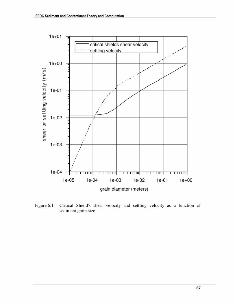
EFDC Sediment and Contaminant Theory and Computation
67
1e-05 1e-04 1e-03 1e-02 1e-01 1e+00
1e-04
1e-03
1e-02
1e-01
1e+00
1e+01
grain diameter (meters)
critical shields shear velocity
settling velocity
Figure 6.1. Critical Shield's shear velocity and settling velocity as a function of
sediment grain size.
EFDC Sediment and Contaminant Theory and Computation
68
7. Cohesive Sediment Settling, Deposition and Resuspension
The settling of cohesive inorganic sediment and organic particulate material is an
extremely complex process. Inherent in the process of gravitational settling is the process
of flocculation, where individual cohesive sediment particles and particulate organic
particles aggregate to form larger groupings or flocs having settling characteristics
significantly different from those of the component particles (Burban et al., 1989; 1990;
Gibbs, 1985; Mehta et al., 1989). Floc formation is dependent upon the type and
concentration of the suspended material, the ionic characteristics of the environment, and
the fluid shear and turbulence intensity of the flow environment. Progress has been made
in first principles mathematical modeling of floc formation or aggregation, and
disaggregation by intense flow shear (Lick and Lick, 1988; Tsai et al., 1987). However,
the computational intensity of such approaches precludes direct simulation of flocculation
in operational cohesive sediment transport models for the immediate future.
An alternative approach, which has met with reasonable success, is the parameterization
of the settling velocity of flocs in terms of cohesive and organic material fundamental
particle size, d; concentration, S; and flow characteristics such as vertical shear of the
horizontal velocity, du/dz, shear stress, Avdu/dz, or turbulence intensity in the water
column or near the sediment bed, q. This has allowed semi-empirical expressions having
the functional form
, , ,se se
duW W d S q
dz
=
(7.1)
to be developed to represent the effective settling velocity. A widely used empirical
expression, first incorporated into a numerical by Ariathurai and Krone (1976), relates the
effective settling velocity to the sediment concentration:
a
s so
o
Sw w
S
=
(7.2)
with the o superscript denoting reference values. Depending upon the reference
concentration and the value of α, this equation predicts either increasing or decreasing
settling velocity as the sediment concentration increases. Equation (7.2) with user
defined base settling velocity, concentration and exponent is an option in the EFDC
model. Hwang and Mehta (1989) proposed
( )2 2
n
s m
aSw
S b=
+
(7.3)
based on observations of settling at six sites in Lake Okeechobee. This equation has a
general parabolic shape with the settling velocity decreasing with decreasing
EFDC Sediment and Contaminant Theory and Computation
69
concentration at low concentrations and decreasing with increasing concentration at high
concentration. Least squares analysis for the parameters, a, m, and n, in (7.3) was shown
to agree well with observational data. Equation (7.3) does not have a dependence on
flow characteristics, but is based on data from an energetic field condition having both
currents and high frequency surface waves. A generalized form of (7.3) can be selected
as an option in the EFDC model.
Ziegler and Nisbet (1994, 1995) proposed a formulation to express the effective settling
as a function of the floc diameter, df
b
s fw ad= (7.4)
with the floc diameter given by:
1/ 2
2 2
f
f
xz xz
dS
α
τ τ
= +
(7.5)
where S is the sediment concentration, αf is an experimentally determined constant and
τxz and τyz are the x and y components of the turbulent shear stresses at a given position in
the water column. Other quantities in (7.4) have been experimentally determined to fit
the relationships:
( )0.85
2 2
1 xz xza B S τ τ
−
= + (7.6)
( )2 2
20.8 0.5logxz xz
b S Bτ τ= − − −+ (7.7)
where B1 and B2 are experimental constants. This formulation is also an option in the
EFDC model.
A final settling option in EFDC is based on that proposed by Shrestha and Orlob (1996).
The formulation in EFDC has the form
( )exp 4.21 0.147
0.11 0.039
sw S G
G
α
α
= − +
= +
(7.8)
where
( ) ( )2 2
z zG u v∂ ∂= +
(7.9)
is the magnitude of the vertical shear of the horizontal velocity. It is noted that all of
these formulations are based on specific dimensional units for input parameters and
EFDC Sediment and Contaminant Theory and Computation
70
predicted settling velocities and that appropriate unit conversion are made internally in
their implementation in the EFDC model.
Water column-sediment bed exchange of cohesive sediments and organic solids is
controlled by the near bed flow environment and the geomechanics of the deposited bed.
Net deposition to the bed occurs as the flow-induced bed surface stress decreases. The
most widely used expression for the depositional flux is:
:
0 :
cd bs d s d d b cd
cd
d
o
b cd
w S w T S
J
τ ττ τ
τ
τ τ
−− = − ≤
= ≥
(7.10)
where τb is the stress exerted by the flow on the bed, τcd is a critical stress for deposition
which depends on sediment material and floc physiochemical properties (Mehta et al.,
1989) and Sd is the near bed depositing sediment concentration. The critical deposition
stress is generally determined from laboratory or in situ field observations and values
ranging form 0.06 to 1.1 N/m2 have been reported in the literature. Given this wide range
of reported values, in the absence of site specific data the depositional stress and is
generally treated as a calibration parameter. The depositional stress is an input parameter
in the EFDC model.
Since the near bed depositing sediment concentration in (7.10) is not directly calculated,
the procedures of Chapter 5 can be applied to relate the near bed depositional
concentration to the bottom layer or depth averaged concentration. Using (6.14) the near
bed concentration during times of deposition can be determined in terms of the bottom
layer concentration for three-dimensional model applications. Inserting (7.10) into (6.14)
and evaluating the constant at a near bed depositional level gives
( )1R
dd d dR
zS T T S
z
= + −
(7.11)
Integrating (7.11) over the bottom layer gives
( )( )
( )
( )( )( )( )
( )
11
1
11
1
1
ln1 : 1
1
11 : 1
1 1
d
d d d
d
R
eq
d d d
d
zS T T S R
z
zS T T S R
R z
−−
−
−−−
−
∆ = + − = ∆ −
∆ −
= + − ≠ − ∆ −
(7.12)
EFDC Sediment and Contaminant Theory and Computation
71
The corresponding quantities in the numerical solution bottom boundary condition (3.6)
are
( )( )
( )
( )( )( ) ( )
( )
11
1
11
1
1
ln1 : 1
1
11 : 1
1 1
d
d s d d s
d
R
eq
d s d d s
d
zP w T T w R
z
zP w T T w R
R z
−−
−
−−−
−
∆ = + − = ∆ −
∆ −
= + − ≠ − ∆ −
(7.13)
For depth averaged model application, (7.10) is combined with (6.25) and the constant of
integration is evaluated at a near bed depositional level to give
( ) ( )1 1 1
1 1
R
d dd d d d R
Rz zRzS T S T S
R R z
= − + − − + +
(7.14)
Integrating (7.14) over the depth gives
( )( )
( )( )
( )( )
( )( )
( )( )( ) ( )
11
1
11
1
ln2 1 1 11 : 1
2 1 11
12 11 1 : 1
2 1 11 1
dd d
d d d
d
R
dd dd d d
d
zR z R zS T T S R
R Rz
zR z RzS T T S R
R RR z
−−
−
−−
−
+ − + − = + − = + +−
− + − = + − − ≠ + +− −
(7.15)
The corresponding quantities in the numerical solution bottom boundary condition (3.6)
are
( )( )
( )( )
( )( )
( )( )
( )( )( ) ( )
11
1
11
1
ln2 1 1 11 : 1
2 1 11
12 11 1 : 1
2 1 11 1
dd d
d s d d s
d
R
dd dd s d d s
d
zR z R zP w T T w R
R Rz
zR z RzP w T T w R
R RR z
−−
−
−−
−
+ − + − = + − = + +−
− + − = + − − ≠ + +− −
(7.16)
It is noted that the assumptions used to arrive at the relationships, (7.12) and (7.15) are
more tenuous for cohesive sediment than the similar relationships for noncohesive
sediment. The settling velocity for cohesive sediment is highly concentration dependent
and the use of a constant settling velocity to arrive at (7.12) and (7.15) is questionable.
The specification of an appropriate reference level for cohesive sediment is difficult. One
EFDC Sediment and Contaminant Theory and Computation
72
possibility is to relate the reference level to the floc diameter using (7.5). An alternative
is to set the reference level to a laminar sublayer thickness
( )
*
d
Sz
Hu
ν=
(7.17)
where ν(S) is a sediment concentration dependent kinematic viscosity and the water
depth is included to non-dimensionalize the reference level. A number of investigators,
including Mehta and Jiang (1990) have presented experimental results indicating that at
high sediment concentrations, cohesive sediment-water mixtures behave as high viscosity
fluids. Mehta and Jain's results indicate that a sediment concentration of 10,000 mg/L
results in a viscosity ten time that of pure water and that the viscosity increases
logarithmically with increasing mixture density. Use of the relationships (7.12) and
(7.16) is optional in the EFDC model. When they are used, the reference height is set
using (7.17) with the viscosity determined using Mehta and Jain's experimental
relationship between viscosity and sediment concentration. To more fully address the
deposition prediction problem, a nested sediment, current and wave boundary layer
model based on the near bed closure presented in Chapter 4 is under development.
Cohesive bed erosion occurs in two distinct modes, mass erosion and surface erosion.
Mass erosion occurs rapidly when the bed stress exerted by the flow exceeds the depth
varying shear strength, τs, of the bed at a depth, Hme, below the bed surface. Surface
erosion occurs gradually when the flow-exerted bed stress is less than the bed shear
strength near the surface but greater than a critical erosion or resuspension stress, τce,
which is dependent on the shear strength and density of the bed. A typical scenario under
conditions of accelerating flow and increasing bed stress would involve first the
occurrence of gradual surface erosion, followed by a rapid interval of mass erosion,
followed by another interval of surface erosion. Alternately, if the bed is well
consolidated with a sufficiently high shear strength profile, only gradual surface erosion
would occur. Transport into the water column by mass or bulk erosion can be expressed
in the form
( )me s br
o r r
me
mJ w S
T
τ τ≤= =
(7.18)
where Jo is the erosion flux, the product wrSr represents the numerical boundary condition
(3.6), mme is the dry sediment mass per unit area of the bed having a shear strength, τs,
less than the flow-induced bed stress, τb, and Tme is a somewhat arbitrary time scale for
the bulk mass transfer. The time scale can be taken as the numerical model integration
time step (Shrestha and Orlob, 1996). Observations by Hwang and Mehta (1989) have
indicated that the maximum rate of mass erosion is on the order of 0.6 gm/s-m2 which
provides a means of estimating the transfer time scale in (4.10). The shear strength of the
cohesive sediment bed is generally agreed to be a linear function of the bed bulk density
(Mehta et al., 1982; Villaret and Paulic, 1986; Hwang and Mehta, 1989).
EFDC Sediment and Contaminant Theory and Computation
73
s s b sa bρτ = + (7.19)
For the shear strength in N/m2 and the bulk density in gm/cm
3, Hwang and Mehta (1989)
give as and bs values of 9.808 and -9.934 for bulk density greater than 1.065 gm/cm3.
The EFDC model currently implements Hwang and Mehta's relationship, but can be
readily modified to incorporate other functional relationships.
Surface erosion is generally represented by relationships of the form
:r e b ceo r r b ce
ce
dmJ w S
dt
ατ τ
τ ττ
−= = ≥
(7.20)
or
exp :r e b ceo r r b ce
ce
dmJ w S
dt
γ
βτ τ
τ ττ
− = = − ≥
(7.21)
where dme/dt is the surface erosion rate per unit surface area of the bed and τce is the
critical stress for surface erosion or resuspension. The critical erosion rate and stress and
the parameters α, β, and γ are generally determined from laboratory or in situ field
experimental observations. Equation (7.20) is more appropriate for consolidated beds,
while (7.21) is appropriate for soft partially consolidated beds. The base erosion rate and
the critical stress for erosion depend upon the type of sediment, the bed water content,
total salt content, ionic species in the water, pH and temperature (Mehta et al., 1989) and
can be measured in laboratory and sea bed flumes.
The critical erosion stress is related to but generally less than the shear strength of the
bed, which in turn depends upon the sediment type and the state of consolidation of the
bed. Experimentally determined relationships between the critical surface erosion stress
and the dry density of the bed of the form
d
ce scρτ = (7.22)
have been presented (Mehta et al., 1989). Hwang and Mehta (1989) proposed the
relationship
( )b
ce b la cρ ρτ = − + (7.23)
between the critical surface erosion stress and the bed bulk density with a, b, c, and ρl
equal to 0.883, 0.2, 0.05, and 1.065, respectively for the stress in N/m2 and the bulk
density in gm/cm3. Considering the relationship between dry and bulk density
EFDC Sediment and Contaminant Theory and Computation
74
( )( )
b w
d s
s w
ρ ρρ ρ
ρ ρ
−=
−
(7.24)
equations (7.22) and (7.23) are consistent. The EFDC model allow for a user defined
constant critical stress for surface erosion or the use of (7.23). Alternate predictive
expression can be readily incorporated into the model.
Surface erosion rates ranging from 0.005 to 0.1 gm/s-m2 have been reported in the
literature, and it is generally accepted that the surface erosion rate decreases with
increasing bulk density. Based on experimental observations, Hwang and Mehta (1989)
proposed the relationship
10
0.198log 0.23exp
1.0023
e
b
dm
dt ρ
=
−
(7.25)
for the erosion rate in mg/hr-cm2 and the bulk density in gm/cm
3. The EFDC model
allows for a user defined constant surface erosion rate or predicts the rate using (7.25).
Alternate predictive expression can be readily incorporated into the model. The use of
bulk density functions to predict bed strength and erosion rates in turn requires the
prediction of time and depth in bed variations in bulk density which is related to the water
and sediment density and the bed void ratio by
1
1 1b w s
ερ ρ ρ
ε ε
= +
+ +
(7.26)
Selection of the bulk density dependent formulations in the EFDC model requires
implementation of a bed consolidation simulation to predict the bed void ratio as
discussed in the following chapter.
EFDC Sediment and Contaminant Theory and Computation
75
8. Sorptive Contaminant Transport
The transport of a sorptive contaminant in the water column is governed by transport
equations for the contaminant dissolved in the water phase, for the contaminant sorbed to
material effectively dissolved in the water phase, and for the contaminant sorbed to
suspended particles. For the portion of the contaminant dissolved directly in the water
phase
( ) ( ) ( ) ( )
( ) ( )
( ) ( )
( ) ( )
ˆ
ˆ
t x y w x y w y x w z x y w
i i i j j jbz x y z w x y dS S dD D
i j
i i i iwaS w S S
i
x y
j j j jwaD w D D w
j
m m HC m HuC m HvC m m wC
Am m C m m H K S K D
H
CK S
m m HC
K D C
∂ ∂ ∂ ∂
∂ ∂ χ χ
ψ χ χφ
ψ χ χ γφ
+ + +
= + +
−
− + − +
∑ ∑
∑
∑
(8.1)
where Cw is the mass of water dissolved contaminant per unit total volume, χS is the
mass of contaminant sorbed to sediment class i per mass of sediment, χD is the mass of
contaminant sorbed to dissolved material j per unit mass of dissolved material, φ is the
porosity, ψw is the fraction of the water dissolved contaminant available for sorption, Ka
is the adsorption rate, Kd is the desorption rate, and γ is a net linearized decay rate
coefficient. The sorption kinetics are based on the Langmuir isotherm (Chapra, 1997)
with χ̂ denoting the saturation sorbed mass per carrier mass. The sediment and dissolved
material concentrations, S and D are defined as mass per unit total volume. The transport
equation for the portion of material sorbed to a dissolved constituent D is,
( ) ( ) ( ) ( )
( ) ( ) ( )
( )( )
ˆ
j j j j j j j j
t x y D x y D y x D z x y D
j j j j j jb wz x y z D x y sD w D D
j j j
x y dD D
m m HD m HuD m HvD m m wD
A Cm m D m m H K D
H
m m H K D
∂ χ ∂ χ ∂ χ ∂ χ
∂ ∂ χ ψ χ χφ
γ χ
+ + +
= + −
− +
(8.2)
The transport equation for the portion of material sorbed to a suspended constituent S is,
( ) ( ) ( ) ( )
( ) ( )
( ) ( ) ( )( )ˆ
i i i i i i i i
t x y S x y S y x S z x y S
i i i i ibz x y S S z x y z S
i i i i i i iwx y aS w S S x y dS S
m m HS m HuS m HvS m m wS
Am m w S m m S
H
Cm m H K S m m H K S
∂ χ ∂ χ ∂ χ ∂ χ
∂ χ ∂ ∂ χ
ψ χ χ γ χφ
+ + +
+ =
+ − − +
(8.3)
EFDC Sediment and Contaminant Theory and Computation
76
Introducing sorbed concentrations defining sorbed mass per unit total volume
j j j
D DC D χ= (8.4)
i i i
S SC S χ= (8.5)
Allows equations (8.1) through (8.3) to be written as
( ) ( ) ( ) ( )
( ) ( )
( ) ( )
( ) ( )
ˆ
ˆ
t x y w x y w y x w z x y w
i i j jbz x y z w x y dS S dD D
i j
i i i iwaS w S S
i
x y
j j j jwaD w D D w
j
m m HC m HuC m HvC m m wC
Am m C m m H K C K C
H
CK S
m m HC
K D C
∂ ∂ ∂ ∂
∂ ∂
ψ χ χφ
ψ χ χ γφ
+ + +
= + +
−
− + − +
∑ ∑
∑
∑
(8.6)
( ) ( ) ( ) ( )
( ) ( )
( )
ˆ
j j j j
t x y D x y D y x D z x y D
j j j j jb wz x y z D x y sD w D D
j j
x y dD D
m m HC m HuC m HvC m m wC
A Cm m C m m H K D
H
m m H K C
∂ ∂ ∂ ∂
∂ ∂ ψ χ χφ
γ
+ + +
= + −
− +
(8.7)
( ) ( ) ( ) ( )
( )
( ) ( ) ( )ˆ
i i i i
t x y S x y S y x S z x y S
i i ibz x y S S z x y z S
i i i i i iwx y aS w S S x y dS S
m m HC m HuC m HvC m m wC
Am m w C m m C
H
Cm m H K S m m H K C
∂ ∂ ∂ ∂
∂ ∂ ∂
ψ χ χ γφ
+ + +
+ =
+ − − +
(8.8)
The EFDC sorbed contaminant transport formulation currently employees equilibrium
partitioning with the adsorption and desorption terms in (8.7) and (8.8) balancing
( ) ( )ˆj j j j j jwsD w D D dD D
CK D K Cψ χ χ
φ
− =
(8.9)
( ) ( )ˆi i i i i iwaS w S S dS S
CK S K Cψ χ χ
φ
− =
(8.10)
EFDC Sediment and Contaminant Theory and Computation
77
Solving (8.9) and (8.10) for the sorbed to water phase concentration ratios gives
1
1ˆ
ˆ
j j jjD D
D
w w
j j j wD Do Do j
D
j j
j w aD DDo j
dD
C f DP
C f
CP P P
KP
K
φ
χ φ
ψ χ
−
= =
= +
=
(8.11)
1
1ˆ
ˆ
i i iiS S
S
w w
i i i wS So So i
S
i ij w aS S
So i
dS
C f SP
C f
CP P P
KP
K
φ
χ φ
ψ χ
−
= =
= +
=
(8.12)
where P denotes the partition coefficient, and Po is its linear equilibrium value. For
linear equilibrium partitioning, P is set to Po, which in effect approximates ( )-1
terms in
(8.11) and (8.12) by unity. Requiring the mass fractions to sum to unity
1i j
w S D
i j
f f f+ + =∑ ∑ (8.13)
gives
ww i i j j
S D
i j
j j jj D D
D i i j j
S D
i j
i i ii S S
S i i j j
S D
i j
Cf
C P S P D
C P Df
C P S P D
C P Sf
C P S P D
φ
φ
φ
φ
= =+ +
= =+ +
= =+ +
∑ ∑
∑ ∑
∑ ∑
(8.14)
The dissolved concentrations can be alternately expressed by mass per unit volume of the
water phase
EFDC Sediment and Contaminant Theory and Computation
78
:
:
:
ww w
jj D
D w
jJ
w
CC
CC
DD
φ
φ
φ
=
=
=
(8.15)
with (8.14) becoming
:
:
: :
:
:
1w w
i i j J
S D w
i j
j j J
D w D w
i i j J
S D w
i j
i i i
S S
i i j J
S D w
i j
C
C P S P D
C P D
C P S P D
C P S
C P S P D
φ φ
φ φ
φ φ
=+ +
=+ +
=+ +
∑ ∑
∑ ∑
∑ ∑
(8.16)
which is a generalization of Chapra's (1997) formulation for sorption to dissolved and
particulate organic carbon.
Adding equations (8.6), (8.7), and (8.8), using the equilibrium partitioning relationships
(8.9) and (8.10) gives
( ) ( ) ( ) ( )1 1t x y x y y x z x y
x y x y
i i bz x y S S z x y z x y
i
m m HC m HuC m HvC m m wCm m m m
Am m w f C m m C m m H C
H
∂ ∂ ∂ ∂
∂ ∂ ∂ γ
+ + +
− = −
∑
(8.17)
the equation for the total concentration, C. The boundary condition at the water column-
sediment bed interface, z = 0, is
EFDC Sediment and Contaminant Theory and Computation
79
( )
( )
max ,0 max ,0
min ,0 min ,0
max ,0
i ibz S S
i
j
w Diji i SBS
SBS S ii S
SB
j
w Diji i SBS
SBS S dep ii S dep
WC
i
SBB
i
S
AC w f C
H
C CJ
J
C CJ
J
J
∂
χ ερ φ
χ ερ φ
ερ
− −
+
= +
+
+ +
+
∑
∑∑
∑∑
( ) ( )
min ,0
max ,0 min ,0
j
w D
j
i
SB
j
w DijSBB
dep ii S dep
WC
j j
w D w D
j j
w w
dep
SB WC
j
w D
j
dif
C C
C CJ
C C C C
q q
C C
q
φ
ερ φ
φ φ
φ
+
+
+
+ +
+ +
+
−
∑∑
∑∑
∑ ∑
∑ j
w D
j
dep
WC SB
C C
φ
+
−
∑
(8.18)
where JSBS and JSBB are the suspended load and bedload sediment fluxes between the
sediment bed and the water column, defined as positive from the bed, ρs is the sediment
density, qw is the water specific discharge due to bed consolidation and groundwater
interaction, defined as positive from the bed, and qdif is a diffusion velocity incorporating
the effects of molecular diffusion, hydrodynamic dispersion, and biological induced
mixing. The subscript SB denotes conditions in the top layer of the sediment bed, while
the subscript WC denotes condition in the water column immediately above the bed, with
the exception that the specific discharge and diffusion velocity are defined at the water
column-bed interface. The subscript, dep, is used to denote the void ratio and porosity of
newly depositing sediment. Equation (8.16) indicates that contaminant flux between the
bed and water column includes, a flux of suspended sediment sorbed material; fluxes of
water dissolved and sorbed to water dissolved material due to the specific discharge of
water associated with consolidation and ground water interaction and water entrainment
and expulsion associated with both suspended and bedload sediment deposition and
resuspension; and a flux of water dissolved and sorbed to water dissolved material due to
diffusion like processes. Transport of bedload sediment sorbed material is represented by
direct transport between horizontally adjacent top bed layers and is included in the
EFDC Sediment and Contaminant Theory and Computation
80
contaminant mass conservation equations for the sediment bed. The boundary condition
at the water free surface is
0 : 1i ibz S S
i
AC w f C z
H∂− − = =∑
(8.19)
Using the relationship between the porosity and void ratio
1
εφ
ε=
+
(8.20)
and (8.5) allows (8.18) to be written as
( )
( )
( )
max ,0 1 max ,0
min ,0 1 min ,0
1 max ,0
i ib
z S S
i
i ii jS SBSSBS w Di i
i jSSB
i ii jS SBSSBS dep w Di i
i jSWC
i
SBB
i
S
AC w f C
H
C JJ C C
S
C JJ C C
S
J
∂
ερ
ερ
ερ
− −
= + + +
+ + + +
+ +
∑
∑ ∑
∑ ∑
( )
( )( )
( )( )
1 min ,0
1max ,0
1min ,0
j
w D
i jSB
ijSBB
dep w Dii jS
WC
j
w dif w D
jSB
j
w dif w D
jWC
C C
JC C
q q C C
q q C C
ερ
φ
φ
+
+ + +
+ + +
+ − +
∑ ∑
∑ ∑
∑
∑
(8.21)
The sediment concentration can be expressed in terms of the sediment density and void
ratio by
1
i ii s
FS
ρ
ε=
+
(8.22)
where Fi is the fraction of the total sediment volume occupied by each sediment class
EFDC Sediment and Contaminant Theory and Computation
81
1i i
i
i ii s s
S SF
ρ ρ
−
=
∑
(8.23)
Introducing (8.14) and (8.22) into (8.21) gives the final form of the bottom boundary
condition
( )
max ,0 max ,0
min ,0 min ,0
1 max ,0
i ibz S S
i
i i i ijSBS S SBS
w Di ii j
SB
i ii idep SBS jSBS S
w Di ii jdep
WC
i
SBBwi
S
AC w f C
H
J f F JC f f C
S S
F JJ fC f f C
S S
JC
∂
ερ
− −
= + +
+ + +
+ +
∑
∑ ∑
∑ ∑
( )
( )( )
( )( )
1 min ,0
1max ,0
1min ,0
j
D
i jSB
ijSBB
dep w Dii jS
WC
j
w dif w D
jSB
j
w dif w D
jWC
C
JC C
q q f f C
q q f f C
ερ
φ
φ
+
+ + +
+ + +
+ − +
∑ ∑
∑ ∑
∑
∑
(8.24)
Note that the form of the bed flux associated with bedload transport remains unmodified
since a sediment concentration in the water column cannot be readily defined for
sediment being transported as bedload.
The transport equation (8.17) for the total contaminant concentration in the water column
is solved using a fractional step procedure which sequentially treats advection; settling,
deposition, and resuspension; pore water advection and diffusion; and reactions. The
fractional phase distribution of the contaminant is recalculated between the advection,
settling, deposition and resuspension, and pore water advection and diffusion steps using
(8.14). The advection step is
( ) ( ) ( ) ( ) ( )1/ 4
0n n
x y y x z
x y x y
HC HC m HuC m HvC wCm m m m
θ θ∂ ∂ θ∂
+− + + + =
(8.25)
with the vertical boundary conditions
0 : 0 , 1wC z= = (8.26)
EFDC Sediment and Contaminant Theory and Computation
82
The fractional time level in (8.25) and subsequent equations is used to denote an
intermediate result in the fractional step procedure. The spatially discrete from of (8.25)
is solved using one of the standard high order, flux limited, advective transport solvers in
the EFDC model.
The settling, deposition, and resuspension step is
( ) ( )1/ 2 1/ 4n n i i
z S S
i
HC HC w f Cθ∂+ +
− = ∑
(8.27)
with the boundary conditions
( )
max ,0 max ,0
min ,0 min ,0
1 max ,0
i i
S S
i
i i i ijSBS S SBS
w Di ii j
SB
i ii idep SBS jSBS S
w Di ii jdep
WC
ijSBB
w DijS
w f C
J f F JC f f C
S S
F JJ fC f f C
S S
JC Cε
ρ
− =
+ +
+ + +
+ + +
∑
∑ ∑
∑ ∑
∑
( )1 min ,0 : 0
iSB
ijSBB
dep w Dii jS
WC
JC C zε
ρ
+ + + =
∑
∑ ∑
(8.28)
0 : 1i i
S Sw f C z= = (8.29)
Integrating (8.27) over a water column layer and using upwind differencing for the
settling gives,
( ) ( )( )
( )
( )( )
1/ 2
1/ 2 1/ 4 1/ 2
1
1
1/ 2
1/ 2
ni i
iSn n nk S
k k ik k ki k
ni i iS nk S
i ki k
w S fHC HC HC
H S
w S fHC
H S
θ
θ
+
+ + ++
+
+
+
+−
∆ − ∆ =
−
∑
∑
(8.30)
for a layer not adjacent to the bed, and,
EFDC Sediment and Contaminant Theory and Computation
83
( ) ( ) ( )1/ 2
1/ 2 1/ 4 1/ 2
1 1 21 1 12
1/ 2
1/ 2max ,0 max ,0
min ,0 min ,0
ni
n n i i nSS i
i
ni i i i
j nSBS S SBSw D sbi i
i jsb
i i i ijSBS S SBS
w Di ij
fHC HC w S C
S
J f J Ff f C
S S
J f J Ff f
S S
θ
θ
θ
+
+ + +
+
+
+
∆ − ∆ =
+ + +
+ + +
∑
∑ ∑
∑
( )
( )
1/ 2
1/ 2
1
1
1/ 2
1/ 2
1/ 2
1/ 2
1
1
1 max ,0
1 min ,0
n
n
i
ni
j nSBBw D sbi
i jS sb
ni
j nSBBw Di
i jS
C
Jf f C
Jf f C
θ ερ
θ ερ
+
+
+
+
+
+
+ + +
+ + +
∑
∑ ∑
∑ ∑
(8.31)
for the first layer adjacent to the bed. Note that (8.31) is also the appropriate form for
single layer or depth average application. Since the sediment settling flux is zero at the
top of the free surface adjacent layer, (8.27) is integrated downward from the top layer to
the bottom layer. The bottom layer equation (8.31) is solved simultaneously with a
corresponding equation for the top layer of the sediment bed. The settling fluxes, wSS,
and water column-sediment bed fluxes, JSB, in (8.30) and (8.31) are known from the
preceding solution for sediment settling, deposition and resuspension. Terms containing
the sediment sorbed fraction divided by the sediment concentration in (8.30) and (8.31)
are given by
i i
S S
i i i j j
S D
i j
f P
S P S P Dφ=
+ +∑ ∑
(8.32)
The diffusion step is given by
( ) ( )3/ 4 1/ 2n n b
z z
AHC HC C
Hθ∂ ∂
+ + − =
(8.33)
with boundary conditions
( )( )
( )( )
1max ,0
1min ,0 : 0
jbz w dif w D
jSB
j
w dif w D
jdep WC
AC q q f f C
H
q q f f C z
∂φ
φ
− = + +
+ − + =
∑
∑
(8.34)
EFDC Sediment and Contaminant Theory and Computation
84
0 : 1bz
AC z
H∂− = =
(8.35)
For the first layer adjacent to the bed
( ) ( )
( )( )
( )( )
3/ 43/ 4 1/ 2
1 111
1/ 2
3/ 4
1
1/ 2
1/ 2
1
1 1
1max ,0
1min ,0
nn n b
z
n
j n
w dif w D SB
jSB
n
j n
w dif w D
j dep
AHC HC C
H
q q f f C
q q f f C
θ∂
θ
φ
θ
φ
++ +
+
+
+
+
+
− =
∆
+ + + ∆
+ − + ∆
∑
∑
(8.36)
It is noted that the bed concentrations are advanced to the n+3/4 intermediate time level
before the advance of the water column concentrations. While for layers not adjacent to
the bed,
( ) ( )3/ 4 3/ 4
3/ 4 1/ 2
1 1
n nn n b b
z zk k
k k
A AHC HC C C
H H
θ θ∂ ∂
+ ++ +
+ −
− = −
∆ ∆
(8.37)
The solution is completed by
( ) ( ) ( )1 3/ 4 1n n n
k k kHC HC HCθγ
+ + +− = − (8.38)
an implicit reaction step.
Contaminant transport in the sediment bed is represented using the discrete layer
formulation developed for bed geomechanical processes. The conservation of mass for
the total contaminant concentration in a layer of the sediment bed is given by
EFDC Sediment and Contaminant Theory and Computation
85
( ) ( )
( ) ( )
( )
( ) ( )( )
, max ,0 max ,0
, min ,0 min ,0
, ,0
,
t k k
i i i ijSBS S SBS
w Di i kti j
kt
i ii iSBS dep jSBS S
w Di ii jdep
WC
i i
SBB SBL
i
BC BC
J f J Fk kt f f BC
BS BS
J FJ fk kt C f f C
S S
k kt J
k k
∂ γ
δ
δ
δ χ
δ
= −
− + +
− + +
−
−
∑ ∑
∑ ∑
∑
( ) ( ) ( )
( ) ( )
( )( ) ( )( )( ) ( )
( ) ( )( )
1 max ,0
, 1 min ,0
1max ,0 min ,0
1, min ,0
ijSBB
w Di kti jS kt
ijSBB
dep w Dii jS WC
j
w dif w dif w D kk kj
k
j
w dif w Dkt
Jt f f BC
B
Jk kt f f C
q q q q f f BCB
k kt q q f f
ερ
δ ερ
φ
δφ
+ −
+
+ +
− + +
− + − − +
− − +
∑ ∑
∑ ∑
∑
( )( ) ( )( ) ( )
( )( ) ( )
1
1
1
1
11 , min ,0
1max ,0
jWC
j
w dif w D kkj
k
j
w dif w D kkj
k
C
k kt q q f f BCB
q q f f BCB
δφ
φ
++
+
−−
−
− − − +
+ + +
∑
∑
∑
(8.39)
where
( )0 :
,1 :
k ktk kt
k ktδ
==
≠
(8.40)
is used to distinguish processes specific to the top, water column adjacent layer of the
bed, kt. Advective fluxes associated with pore water advection in (8.40) are represented
in upwind form. In the sediment bed, the actual computational variables for sediment,
contaminant, and dissolved material are their concentrations times the thickness of the
bed layer. Consistent with this formulation, the fractional phase components in the bed
are defined by
EFDC Sediment and Contaminant Theory and Computation
86
( )
( )
( )
ww i i j jk
k S D
i j k
j j jj D D
D i i j jkS Dk
i j k
i i ii S S
S i i j jkS Dk
i j k
BC Bf
BC B P BS P BD
BC P BDf
BC B P BS P BD
BC P BSf
BC B P BS P BD
φ
φ
φ
φ
= = + +
= = + +
= = + +
∑ ∑
∑ ∑
∑ ∑
(8.41)
The contaminant fluxes associated bedload sediment transport are determined as follows.
The net sediment flux from the bedload transport equation
( ) ( )i i i
x y SBB x y SBLx x x SBLym m J m Q m Q∂ ∂= + (8.42)
is used to evaluate the flux associated with pore water entrainment and expulsion in
(8.25) and (8.40). The transport equation for material sorbed to the bedload is
( ) ( )i i i i i i
x y SBLx SBL x x SBLy SBL x y SBB SBLm Q m Q m m J∂ χ ∂ χ χ+ = (8.43)
Since the contaminant mass per sediment mass in the transport divergence corresponds to
conditions in the top layer of the sediment bed, (8.43) can be written as
i i
i i i iS Sx y SBLx x x SBLy x y SBB SBLi i
f fm Q C m Q C m m J
S S∂ ∂ χ
+ =
(8.44)
and solved using an upwind approximation
( ) ( )
( ) ( )
( ) ( )
( )
max min
max min
max min
max min
i i
x y SB SBL
i ii iS S
y SBLx y SBLxi iE EC E
i ii iS S
y SBLx y SBLxi iW WW C
i ii iS S
x SBLy x SBLyi iN NC N
ii S
x SBLy iSS
m m J
f fm Q C m Q C
S S
f fm Q C m Q C
S S
f fm Q C m Q C
S S
fm Q C m
S
χ =
+
− −
+ +
− −
( )
ii S
x SBLy iSC
fQ C
S
(8.45)
EFDC Sediment and Contaminant Theory and Computation
87
to evaluate the transport of bedload sorbed material between horizontally adjacent top
layers of the sediment bed.
Equation (8.39) is solved using a fractional step procedure consistent with that used for
the water column transport. Equation (8.41) is used to update the fractional distribution
in the bed between the settling, deposition, and resuspension step and the pore water
advection and diffusion step. The settling, deposition and resuspension step applies only
to the top layer of the bed and is
( ) ( )
( )
1/ 2
1/ 2
1/ 2
1/ 2
max ,0 max ,0
min ,0 min ,0
,
n n
kt kt
ni i i i
njSBS S SBSw Di i kt
i jkt
ni ii iSBS dep jSBS S
w Di ii jdep
WC
i i
SBB SBL
BC BC
J f J Ff f BC
BS BS
J FJ fC f f C
S S
J
θ
θ
θ χ
+
+
+
+
− =
− + +
− + +
−
∑ ∑
∑ ∑
( )( )
( ) ( )
( )
1/ 2
1/ 2
1/ 2
0
1 max ,0
1 min ,0
i
ni
njSBBw Di kt
i jS kt
ni
jSBBdep w Di
i jS WC
Jf f BC
B
Jf f C
θ ερ
θ ερ
+
+
+
− + +
− + +
∑
∑ ∑
∑ ∑
(8.46)
This equation is solved simultaneously with equation (8.31) for the bottom layer of the
water column. The solution is represented by
( )
( )
( ) ( )
( ) ( )
1/ 2
1/ 2
11 12
1/ 21/ 221 22 1/ 4 1/ 21
1 21 12
nn i i
SB SBLktn i
i ibkt
nni
n i i nSS i
i
BC J
BCa a
a a HC fHC w S C
S
θ χ
θ
+
+=
++
+ +
+
−
=
∆ +
∑
∑
(8.47)
where the coefficients are given by
EFDC Sediment and Contaminant Theory and Computation
88
( )
1/ 2
11
1/ 2
12
1 max ,0 max ,0
1 max ,0
min ,0 min ,0
ni i i i
jSBS S SBSw Di i
i jkt
ni
jSBBw Di
i jS kt
i ii iSBS dep jSBS S
w Di i
dep
J f J Fa f f
BS BS
Jf f
B
J FJ fa f f
H S S
θ
θ ερ
θ
+
+
= + + +
+ + +
= + +
∑ ∑
∑ ∑
( )
( )
1/ 2
1
1/ 2
1
1/ 2
21
1 min ,0
max ,0 max ,0
1 max ,0
n
i j
ni
jSBBdep w Di
i jS
ni i i i
jSBS S SBSw Di i
i jkt
ijSBB
w DijS
Jf f
H
J f J Fa f f
BS BS
Jf f
B
θε
ρ
θ
θ ερ
+
+
+
+ + +
= − + +
− + +
∑ ∑
∑ ∑
∑ ∑
∑
( )
1/ 2
1/ 2
22 1
1
1/ 2
1
min ,0 min ,0
1 min ,0
n
ikt
ni i i i
jSBS S SBSw Di i
i j
ni
jSBBw Di
i jS
J f J Fa f f
H S S
Jf f
H
θ
θε
ρ
+
+
+
= ∆ − + +
− + +
∑
∑ ∑
∑ ∑
(8.48)
Adding the two equations in (8.47) gives
( ) ( ) ( ) ( )
( ) ( )
1/ 2 1/ 2 1/ 4
1 11 1
1/ 2
1/ 21/ 2
212
n n n n
kt kt
ni
ni i n i iSS SBS SBLi
i i
BC HC BC HC
fw S C J
Sθ θ χ
+ + +
+
++
+
+ ∆ = + ∆
+ − ∑ ∑
(8.49)
This equation verifies the consistency of the water column-sediment bed exchange since
the source and sinks on the right side include only settling into the top of the water
column layer, and transfer of bedload sediment sorbed contaminant between horizontal
sediment bed cells.
The pore water advection and diffusion step for the top, water column adjacent, layer is
EFDC Sediment and Contaminant Theory and Computation
89
( ) ( )
( )( ) ( )
( )( ) ( )
( )( ) ( )
( )
3/ 4 1/ 2
1/ 2
3/ 4
1/ 2
3/ 4
1/ 2
1/ 2
1
1
1max ,0
1min ,0
1min ,0
max ,0
n n
kt kt
n
nj
w dif w D ktktj
kt
n
nj
w dif w D ktktj
kt
n
nj
w dif w Dktj
w
BC BC
q q f f BCB
q q f f BCB
q q f f HCH
q
θφ
θφ
θφ
θ
+ +
+
+
+
+
+
−
+
+
+
=
− + +
+ − +
− − +
+
∑
∑
∑
( ) ( )1/ 2
1/ 2
1
1
1n
nj
dif w D ktktj
kt
q f f BCBφ
+
+
−−
−
+ +
∑
(8.50)
which is an implicit form. Writing (8.36) in the form
( ) ( )
( )( ) ( )
( )( ) ( )
3/ 43/ 4 1/ 2
1 11 11
1/ 2
3/ 4
1/ 2
1/ 2
1
1
1max ,0
1min ,0
nn n b
z
n
nj
w dif w D ktktj
SB
n
nj
w dif w Dktj
AHC HC C
H
q q f f BCB
q q f f HCH
θ ∂
θφ
θφ
++ +
+
+
+
+
+
+
+
∆ = ∆ +
+ + +
+ − +
∑
∑
(8.51)
and combining with (4.49) gives
( ) ( ) ( ) ( )
( )( ) ( )
( )( ) ( )
3/ 43/ 4 3/ 4 1/ 2 1/ 2
1 11 11
1/ 2
3/ 4
1/ 2
3/ 4
1
1
1min ,0
1max ,0
nn n n n b
zkt kt
n
nj
w dif w D ktktj
kt
n
nj
w dif w D ktktj
kt
ABC HC BC HC C
H
q q f f BCB
q q f f BCB
θ ∂
θφ
θφ
++ + + +
+
+
+
−
+
+
−−
−
+ ∆ = + ∆ +
+ − +
+ + +
∑
∑
(8.52)
This equation verifies the consistency of the representation of pore water advection and
diffusion across water column-sediment bed interface since the source and sink terms on
the right side of (8.52) represent fluxes at the top to the water column cell and the bottom
of the bed cell.
The pore water diffusion and advection step for the remaining bed layers is given by
EFDC Sediment and Contaminant Theory and Computation
90
( ) ( )
( )( ) ( )
( )( ) ( )
( )( ) ( )
( )( )
3/ 4 1/ 2
1/ 2
3/ 4
1
1
1/ 2
3/ 4
1/ 2
3/ 4
1min ,0
1max ,0
1min ,0
max ,0
n n
k k
n
nj
w dif w D kkj
k
n
nj
w dif w D kkj
k
n
nj
w dif w D kkj
k
w dif
BC BC
q q f f BCB
q q f f BCB
q q f f BCB
q q
θφ
θφ
θφ
θ
+ +
+
+
++
+
+
+
+
+
+
−
=
− − +
− + +
+ − +
+ +
∑
∑
∑
( )1/ 2
3/ 4
1
1
1n
nj
w D kkj
k
f f BCBφ
+
+
−−
−
+
∑
(8.53)
For the bottom layer of the bed, k = 1, the bottom, k-, specific discharge and diffusion
velocity must be specified as well as the total contaminant concentration, C0. The
corresponding thickness of the unresolved layer, k = 0, is set to unity without loss of
generality. The system of equations represented by (8.49) and (8.52) is implicit and is
solved using a tri-diagonal linear equation solver. It is noted that the n+3/4 time level
layer thickness is actually the n+1 time level thickness determined by the solution of
(8.23). The specific discharges in (8.49) and (8.52) are given by (8.41) and represent
those appearing in (8.23) and guarantee mass conservation for the pore water advection.
The bed transport solution is completed by
( ) ( ) ( )1 3/ 4 1n n n
k k kBC BC BCθγ
+ + +− = − (8.54)
an implicit reaction step.
EFDC Sediment and Contaminant Theory and Computation
91
9. References
Ackers, P., and W. R. White, 1973: Sediment transport: New approaches and analysis. J.
Hyd. Div. ASCE, 99, 2041-2060.
Ariathurai, R., and R. B. Krone, 1976: Finite element model for cohesive sediment
transport. J. Hyd. Div. ASCE, 102, 323-338.
Ambrose, R. B., T. A. Wool, and J. L. Martin, 1993: The water quality analysis and
simulation program, WASP5: Part A, model documentation version 5.1. U.S. EPA,
Athens Environmental Research Laboratory, 210 pp.
Bear, J., 1879: Hydraulics of groundwater, McGraw-Hill, New York.
Bagnold, R. A., 1956: The flow of cohesionless grains in fluids. Phil. Trans. Roy. Soc.
Lond., Series A, Vol 249, No. 964, 235-297.
Belleudy, P., 2001: Numerical simulation of sediment mixture deposition, part 1:
analysis of flume experiments. J. Hyd. Res., 38, 417-425.
Belleudy, P., 2001: Numerical simulation of sediment mixture deposition, part 2: a
sensitivity analysis. J. Hyd. Res., 39, 25-31.
Blumberg, A. F., B. Galperin, and D. J. O'Connor, 1992: Modeling vertical structure of
open-channel flow. J. Hyd. Engr., 118, 1119-1134.
Boyer, J. M., S. C. Chapra, C. E. Ruiz, and M. S. Dortch, 1994: RECOVERY, a
mathematical model to predict the temporal response of surface water to contaminated
sediment. Tech. Rpt. W-94-4, U.S. Army Engineer Waterways Experiment Station,
Vicksburg, MS, 61 pp.
Burban, P. Y., W. Lick, and J. Lick, 1989: The flocculation of fine-grained sediments in
estuarine waters. J. Geophys. Res., 94, 8323-8330.
Burban, P. Y., Y. J. Xu, J. McNeil, and W. Lick, 1990: Settling speeds of flocs in fresh
and seawater. J. Geophys. Res., 95, 18,213-18,220.
Cargill, K. W., 1985: Mathematical model of the consolidation and desiccation processes
in dredge material. U.S. Army Corps of Engineers, Waterways Experiment Station,
Technical Report D-85-4.
Dortch, M., C. Ruiz, T. Gerald, and R. Hall, 1998: Three-dimensional contaminant
transport/fate model. Estuarine and Coastal Modeling, Proceedings of the 5th
International Conference, M. L. Spaulding and A. F. Blumberg, Eds., American Society
of Civil Engineers, New York, 75-89.
EFDC Sediment and Contaminant Theory and Computation
92
Einstein, H. A., 1950: The bed load function for sediment transport in open channel
flows. U.S. Dept. Agric. Tech. Bull., 1026.
Fredricks, C., and J. M. Hamrick, 1996: The effect of channel geometry on gravitational
circulation in partially mixed estuaries. Buoyancy Effects on Coastal and Estuarine
Dynamics, D. Aubrey and C. Fredricks, Eds., AGU, 283-300.
Galperin, B., L. H. Kantha, S. Hassid, and A. Rosati, 1988: A quasi-equilibrium
turbulent energy model for geophysical flows. J. Atmos. Sci., 45, 55-62.
Garcia, M., and G. Parker, 1991: Entrainment of bed sediment into suspension. J. Hyd.
Engrg., 117, 414-435.
Gibbs, R. J., 1985: Estuarine Flocs: their size, settling velocity and density. J. Geophys.
Res., 90, 3249-3251.
Gibson, R. E., G. L. England, and M. J. L. Hussey, 1967: The theory of one-dimensional
consolidation of saturated clays. Geotechnique, 17, 261-273.
Hamrick, J. M., 1992: A three-dimensional environmental fluid dynamics computer
code: Theoretical and computational aspects. The College of William and Mary, Virginia
Institute of Marine Science, Special Report 317, 63 pp.
Hamrick, J. M., 1994: Linking hydrodynamic and biogeochemical transport models for
estuarine and coastal waters. Estuarine and Coastal Modeling, Proceedings of the 3rd
International Conference, M. L. Spaulding et al, Eds., American Society of Civil
Engineers, New York, 591-608.
Hamrick, J. M., and Wm. B. Mills, 2001: Analysis of temperatures in Conowingo Pond
as influenced by the Peach Bottom atomic power plant thermal discharge. Environ. Sci.
Policy, 3, s197-s209.
Hamrick, J. M., and T. S. Wu, 1997: Computational design and optimization of the
EFDC/HEM3D surface water hydrodynamic and eutrophication models. Next
Generation Environmental Models and Computational Methods. G. Delich and M. F.
Wheeler, Eds., Society of Industrial and Applied Mathematics, Philadelphia, 143-156.
Hayter, E. J., and A. J. Mehta, 1983: Modeling fine sediment transport in estuaries.
Report EPA-600/3-83-045, U.S. Environmental Protection Agency. Athens, GA.
Hayter, E.J., M. Bergs, R. Gu, S. McCutcheon, S. J. Smith, and H. J. Whiteley, 1998:
HSCTM-2D, a finite element model for depth-averaged hydrodynamics, sediment and
contaminant transport. Technical Report, U. S. EPA Environmental Research Laboratory,
Athens, GA.
EFDC Sediment and Contaminant Theory and Computation
93
Hwang, K.-N, and A. J. Mehta, 1989: Fine sediment erodibility in Lake Okeechobee.
Coastal and Oceanographic Engineering Dept., University of Florida, Report
UFL/COEL-89/019, Gainesville, FL.
Ji, Z.-G., J. H. Hamrick, and J. Pagenkopf, 2002: Sediment and metals modeling in
shallow river, J. Environ. Engrg., 128, 105-119.
Jin, K. R., J. M. Hamrick, and T. S. Tisdale, 2000: Application of a three-dimensional
hydrodynamic model for Lake Okeechobee, J. Hyd. Engrg., 106, 758-772.
Jin, K. R., Z. G. Ji, and J. M. Hamrick, 2002: Modeling winter circulation in Lake
Okeechobee, Florida. J. Waterway, Port, Coastal, Ocean Engrg., 128, 114-125.
Karim, M. F., and F. M. Holley, Jr., 1986: Armoring and sorting simulation in alluvial
rivers. J. Hyd. Engrg., 112, 705-715.
Kleinhans, M. G., and L. C. Van Rijn, 2002: Stochastic prediction of sediment transport
in sand-gravel bed rivers. J. Hyd. Engrg., 128, 412-425.
Kuo, A. Y., J. Shen, and J. M. Hamrick, 1996: The effect of acceleration on bottom shear
stress in tidal estuaries. J. Waterway, Port, Coastal, Ocean Engrg., 122, 75-83.
Laursen, E., 1958: The total sediment load of streams J. Hyd. Div. ASCE, 84, 1-36.
Letter, J. V., L. C. Roig, B. P. Donnell, Wa. A. Thomas, W. H. McAnally, and S. A.
Adamec, 1998: A user's manual for SED2D-WES, a generalized computer program for
two-dimensional, vertically averaged sediment transport. Version 4.3 Beta Draft
Instructional Report, U. S. Army Corps of Engrs., Wtrwy. Exper. Sta., Vicksburg, MS.
Le Normant, C., E. Peltier, and C. Teisson, 1998: Three-dimensional modelling of
cohesive sediment in estuaries. in Physics of Estuaries and Coastal Seas, (J. Dronkers and
M. Scheffers, Eds.), Balkema, Rotterdam, pp 65-71.
Lick, W., and J. Lick, 1988: Aggregation and disaggregation of fine-grained lake
sediments. J Great Lakes Res., 14, 514-523.
Mehta, A. J., E. J. Hayter, W. R. Parker, R. B. Krone, A. M. Teeter, 1989: Cohesive
sediment transport. I: Process description. J. Hyd. Engrg., 115, 1076-1093.
Mehta, A. J., T. M. Parchure, J. G. Dixit, and R. Ariathurai, 1982: Resuspension potential
of deposited cohesive sediment beds, in Estuarine Comparisons, V. S. Kennedy, Ed.,
Academic Press, New York, 348-362.
Mehta, A. J., and F. Jiang, 1990: Some field observations on bottom mud motion due to
waves. Coastal and Oceanographic Engineering Dept., University of Florida, Gainesville,
FL.
EFDC Sediment and Contaminant Theory and Computation
94
Mellor, G. L., and T. Yamada, 1982: Development of a turbulence closure model for
geophysical fluid problems. Rev. Geophys. Space Phys., 20, 851-875.
Meyer-Peter, E. and R. Muller, 1948: Formulas for bed-load transport. Proc. Int. Assoc.
Hydr. Struct. Res., Report of Second Meeting, Stockholm, 39-64.
Middleton, G. V., and P. R. Wilcock, 1994: Mechanics in the Earth and Environmental
Sciences. Cambridge University Press, Cambridge, UK.
Moustafa, M. Z., and J. M. Hamrick, 2000: Calibration of the wetland hydrodynamic
model to the Everglades nutrient removal project. Water Quality and Ecosystem
Modeling, 1, 141-167.
Nielsen, P., 1992: Coastal bottom boundary layers and sediment transport, World
Scientific, Singapore.
Park, K., A. Y. Kuo, J. Shen, and J. M. Hamrick, 1995: A three-dimensional
hydrodynamic-eutrophication model (HEM3D): description of water quality and
sediment processes submodels. The College of William and Mary, Virginia Institute of
Marine Science. Special Report 327, 113 pp.
Rahmeyer, W. J., 1999: Lecture notes for CEE5560/6560: Sedimentation Engineering,
Dept. of Civil and Environmental Engineering, Utah State University, Logan, Utah.
Rahuel, J. L., F. M. Holly, Jr., J. P. Chollet, P. J. Belleudy, 1990: Modeling riverbed
evolution for bedload sediment mixtures. J. Hyd. Engrg., 115, 1521-1542.
Raukivi, A. J., 1990: Loose boundary hydraulics. 3rd Ed., Pergamon, New York, NY.
Ried, I., and L. E. Frostick, 1994: Fluvial sediment transport and deposition. in Sediment
Transport and Depositional Processes, K. Pye, ed., Blackwell, Oxford, UK, 89-155.
Roberts, J., R. Jepson, D. Gotthard, and W. Lick, 1998: Effects of particle size and bulk
density on erosion of quartz particles. J. Hyd. Engrg., 124, 1261-1267.
Shen, J., J. D. Boon, and A. Y. Kuo, 1999: A modeling study of a tidal intrusion front and
its impact on larval dispersion in the James River estuary, Virginia. Estuaries, 22, 681-
692.
Shen, J. and A.Y. Kuo. 1999: Numerical investigation of an estuarine front and its
associated topographic eddy. J. Waterway, Port, Coastal Ocean Engrg., 125, 127-135.
Shrestha, P. A., and G. T. Orlob, 1996: Multiphase distribution of cohesive sediments and
heavy metals in estuarine systems. J. Environ. Engrg., 122, 730-740.
Smagorinsky, J., 1963: General circulation experiments with the primative equations,
Part I: the basic experiment. Mon. Wea. Rev., 91, 99-152.
EFDC Sediment and Contaminant Theory and Computation
95
Smith, J. D., and S. R. McLean, 1977: Spatially averaged flow over a wavy bed. J.
Geophys. Res., 82, 1735-1746.
Smolarkiewicz, P. K., and T. L. Clark, 1986: The multidimensional positive definite
advection transport algorithm: further development and applications. J. Comp. Phys., 67,
396-438.
Smolarkiewicz, P. K., and W. W. Grabowski, 1990: The multidimensional positive
definite advection transport algorithm: non-oscillatory option. J. Comp. Phys., 86, 355-
375.
Spasojevic, M., and F. M. Holly, Jr., 1990: 2-D bed evolution in natural watercourses-
new simulation approach. J. Hyd. Engrg., 116, 425-443.
Spasojevic, M., and F. M. Holly, Jr., 1994: Three-dimensional numerical simulation of
mobile-bed hydrodynamics. Contract Report HL-94-2, U.S. Army Engineer Waterways
Experiment Station, Vicksburg, MS.
Stark, T. D., 1996: Program documentation and users guide: PSDDF primary
consolidation, secondary compression, and desiccation of dredge fill. Instructional Report
EL-96-xx, US Army Engineer Waterways Experiment Station, Vicksburg, MS.
Styles, R. and S. M. Glenn, 2000: Modeling stratified wave and current boundary layers
on the continental shelf. J. Geophys. Res., 105, 24,119-24,139.
Suzuki, K., H. Yamamoto, and A. Kadota, 1998: Mechanism of bed load fluctuations of
sand-gravel mixture in a steep slope channel, Proc. of the 11th Congress of APD IAHR,
Yogyakarta, pp.679-688.
Tetra Tech, 2007a: The Environmental Fluid Dynamics Code Theory and Computation.
Volume 1: Hydrodynamics and Mass Transport.
Tsai, C. H., S. Iacobellis, and W. Lick, 1987: Flocculation of fine-grained lake sediments
due to a uniform shear stress. J Great Lakes Res., 13, 135-146.
van Niekerk, A., K. R. Vogel, R. L Slingerland, and J. S. Bridge, 1992: Routing of
heterogeneous sediments over movable bed: Model development. J. Hyd. Engrg., 118,
246-262.
Van Rijn, L. C., 1984a: Sediment transport, Part I: Bed load transport. J. Hyd. Engrg.,
110, 1431-1455.
Van Rijn, L. C., 1984b: Sediment transport, Part II: Suspended load transport. J. Hyd.
Engrg., 110, 1613-1641.
EFDC Sediment and Contaminant Theory and Computation
96
Villaret, C., and M. Paulic, 1986: Experiments on the erosion of deposited and placed
cohesive sediments in an annular flume and a rocking flume. Coastal and Oceanographic
Engineering Dept., University of Florida, Report UFL/COEL-86/007, Gainesville, FL.
Vogel, K. R., A. van Niekerk, R. L Slingerland, and J. S. Bridge, 1992: Routing of
heterogeneous sediments over movable bed: Model verification. J. Hyd. Engrg., 118,
263-279.
Wu, W., S. S. Y. Wang, and Y. Jia, 2000: Nonuniform sediment transport in alluvial
rivers. J. Hyd. Res., 38, 427-434.
Yang, C. T., 1973: Incipient motion and sediment transport. J. Hyd. Div. ASCE, 99, 1679-
1704.
Yang, C. T., 1984: Unit stream power equation for gravel. Journal of Hydraulic
Engineering, 110, 1783-1797.
Yang, C. T., and A. Molinas, 1982: Sediment transport and unit streams power function.
J. Hyd. Div. ASCE, 108, 774-793.
Yang, Z., A. Baptista, and J. Darland, 2000: Numerical modeling of flow characteristics
in a rotating annular flume. Dyn. Atmos. Oceans, 31, 271-294.
Ziegler, C. K., and B. Nesbitt, 1994: Fine-grained sediment transport in Pawtuxet River,
Rhode Island. J. Hyd. Engrg., 120, 561-576.
Ziegler, C. K., and B. Nesbitt, 1995: Long-term simulation of fine-grained sediment
transport in large reservoir. J. Hyd. Engrg., 121, 773-781.