Efficient Function Evaluations with Lookup Tables forStructured Matrix Operations

Kanwaldeep Sobti, Lanping Deng, Chaitali Chakrabarti, Nikos Pitsianis and Xiaobai Sun

October 16, 2006

Department of Computer ScienceDuke University

Technical Report CS-2006-13

2

Efficient Function Evaluations with Lookup Tablesfor Structured Matrix Operations

Kanwaldeep Sobti, Lanping Deng, Chaitali Chakrabarti, Nikos Pitsianis and Xiaobai Sun

Abstract— A hardware-efficient approach is introduced forextensive function evaluations in certain structured matrixcomputations. It is a comprehensive approach that utilizeslookup tables for their relatively low utilization of hardwareresources, employs interpolations with adders and multipliers fortheir adaptivity to non-tabulated values and, more distinctively,exploits the function properties and the matrix structures to claimbetter control over numerical dynamic ranges. This approachbrings forth more opportunities and room for improvementin hardware efficiency without compromising latency andnumerical accuracy. We demonstrate the effectiveness of theapproach with simulation results on evaluating, in particular,the cosine function, the exponential function and the zero-orderBessel function of the first kind.

.Keywords: computer arithmetic, elementary function eval-uation, lookup-table based algorithms, structured matrices,geometric tiling

I. INTRODUCTION

This paper introduces efficient techniques for hardware im-plementation of accurate function evaluation via the integrateddesign of lookup tables and lookup schemes. The functions ofinterest include mathematical elementary and special functionsused often in real-time digital signal processing or large-sizesimulation in scientific and engineering studies. In particu-lar, we have used the techniques for efficiently evaluatingtrigonometric functions, square-root extraction, logarithmicexponential function, and more complex functions such as theBessel functions. Conventionally, most of these functions areevaluated in software, with no lookup table or with lookuptables of different sizes based on the available memory space.The overhead in both memory and latency associated withsoftware implementation is often too high to meet the highspeed and high throughput requirement. In hardware imple-mentation, there are also additional requirements on power andarea consumption. The use of lookup tables is an importantcomponent in both algorithmic and architectural domains. It isan effective, and sometimes necessary, scheme to utilize pre-computed tabulated data for function evaluation, especially atnon-tabulated locations, with fewer operations and within arequired accuracy. In hardware implementation, lookup table

Manuscript received ??, 2006; revised ??, 2006.K. Sobti, L. Deng and C. Chakrabarti are with Department of Electrical

Engineering, Arizona State UniversityN. Pitsianis is with the Department of Electrical Engineering, Duke

UniversityX. Sun is with the Department of Computer Science, Duke University.

technique can use small area since the memory is much denserthan logic modules such as adders and multipliers [2].

The ultimate goal is to have accurate function evaluationswith fast lookup schemes and small lookup tables. There is,however, a tangled relationship among the latency, accuracyand memory size. For example, in a straightforward or directtable lookup scheme, a higher-accuracy evaluation requires afiner sampling for table entries and hence a larger table. Whilesuch direct lookup scheme is generally believed to be fast, thegrowth in table size may be exponential with the number ofrequired accurate digits, not only consuming large memoryspace but also subsuming the lookup mechanism and speed.

The techniques we introduce in this paper are developedto explore the latency-accuracy-resource design space forcombined reduction or minimization in memory and latencysubject to an accuracy constraint. Furthermore, to narrow theconventional ’tradeoff’ among the three issues, we find ’pay-off’ by exploring and exploiting the structures in applicationenvironments where the function evaluations are requested.Specifically, we consider the basic matrix operations witha class of structured matrices that are certain transforms indiscrete format and appear commonly in signal and imageprocessing, in data or information processing, and in manyscientific and engineering simulations. We explore and exploitthe geometric and analytic structures of the transformationkernel functions and the associated discrete data sets.

The rest of the paper is organized as below. In Section IIwe provide preliminary approaches for exploring the designspace and describe the structured matrices we are interestedin. In Section III we describe our approach to exploiting thegeometric structures of the kernel functions in matrix evalu-ations, which are to be followed by the discrete transforms,i.e., matrix-vector multiplications in the case of linear trans-forms. In Section IV we introduce a new hardware-efficientinterpolation scheme to be used together with fast table-lookup for function evaluation to higher accuracy adaptively.We then demonstrate in Section V the effectiveness of theintroduced approaches. We conclude the paper in Section VIwith discussion on other related issues.

II. PRELIMINARIES

We introduce first certain pre-processing, interlacing cal-culation and post-processing approaches which exploit themathematical properties of the functions to be evaluated. Thishelps to reduce the size of lookup table. We then describethe structured matrices of our interest, for which efficient andaccurate function evaluations at large data sets are required.

3

A. Reduction in lookup table size

In preprocessing, one may reduce the dynamic range of theinput by variable folding or/and scaling. In folding, when ap-plicable, the entire dynamic range of the input is folded onto amuch smaller range. For trigonometric functions, for example,the folding can be based on the trigonometric identities suchas

sin(2nπ + u) = sin(u), cos(2nπ + u) = cos(u);

sin(2u) = 2 sin(u) cos(u), cos(2u) = 2 cos2(u) − 1. (1)

For the exponential function, we may use αx = αx/2 · αx/2

to reduce the initial range by a factor of 2, at the expenseof a shift in the input and a multiplication at the output. Forsome other functions such as power functions, one may usemultiplicative change in the input variable, i.e., variable scalingto reduce the dynamic range,

xβ = cβ(x/c)β . (2)

The power functions include in particular the division (β =−1) and the square root (β = 1/2). The folding and scalingcan be performed in either hardware or software. Equation (2)already includes the scaling recovery in the post-processing,where cβ is pre-selected and pre-evaluated. Both folding,scaling, their reverse operations, and the associated overheadshall be taken into consideration in the design and developmentof table construction and lookup,

Between the preprocessing and postprocessing, the tablelookups may be tightly coupled with interpolations to adap-tively meet accuracy requirements without increasing the tablesize. A simple example is the approximation of a function f ata non-entry value x by a linear interpolation of two tabulatedneighbor values f(x1) and f(x2) such that x1 < x < x2,

f(x) ≈ f(x1) +f(x2) − f(x1)

x2 − x1(x − x1).

If higher accuracy is required, one may use a higher-orderinterpolation scheme.

Two particular interpolation schemes are considered in thispaper. One requires pre-computed derivatives for every tableentry, based on Taylor’s series expansion and truncation.The other uses finite divided differences, based on Newton’sinterpolation approach [4]. Mathematically, both the schemesrender a polynomial approximation of a specified degree. Inerror analysis, both the schemes have similar error estimates.But they do differ in interpolation locality, in requirement forpre-computed quantities, in look-up table construction. Theyalso represent a tradeoff between memory space and lookuplatency in certain situation .

We give a brief review of the two interpolation schemes.According to Taylor’s theorem [3], a function f at x can beapproximated by a Taylor polynomial of degree n,

Tn(x) =

n∑

k=0

f (k)(x0)

k!(x − x0)

k, (3)

where x0 indicates a table entry, the function is assumedsmooth enough at x0 to warrant the existence of the derivatives

at x0. The approximation error is described as follows,

Rn(x) =f (n+1)(ξ(x))

(n + 1)!(x − x0)

n+1, (4)

where ξ(x) is between x0 and x. One determines from theerror estimates the minimal approximation degree n, takinginto consideration the sample space between table entries andthe behavior of the higher order derivatives. The formationof the Taylor polynomial in (3) requires not only tabulatingf(x0) but also the derivatives at x0 up to the n order.

In Newton’s interpolation scheme, only the tabulated func-tion values, not the derivatives, are explicitly required. Butmore number of tabulated function values are used for theapproximation of f at x, and the number of such referencepoints increases with the higher accuracy requirement. Assumethat function f(x) is to be evaluated at point x and the functionhas already been sampled at points s0, s1, · · · , sk. Then, f(x)is approximated by the following polynomial,

Nn(x) = f [s0] + f [s0, s1](x − s0)

+ f [s0, s1, s2]

1∏

j=0

(x − sj) + · · ·

+ f [s0, s1, · · · , sn]

n−1∏

j=0

(x − sj).

(5)

Similarly to the Taylor polynomial, the i-th term in the Newtonpolynomial is a polynomial of degree i. In place of the i-thderivative divided by i!, here we have the i-th order divideddifference, which can be computed recursively from those oflower orders and all the way from the function values,

f [s0] = f(s0),

f [s0, s1] =f [s1] − f [s0]

s1 − s0,

f [s0, s1, s2] =f [s1, s2] − f [s0, s1]

s2 − s0,

...

f [s0, · · · , sk] =f [s1, · · · , sk] − f [s0, · · · , sk−1]

sk − s0.

The approximation error in Nn may be described as follow,

En(x) = f [s0, · · · , sn, x]n∏

j=0

(x − sj)

=1

(n + 1!)f (n+1)(ξ)

n∏

j=0

(x − sj), (6)

where ξ is between minj=0:n sj and maxj=0:n sj .The above interpolation schemes can be easily found in text

books on numerical analysis, see [4] for instance. They repre-sent the extreme cases in reference locality for any specifiedpolynomial degree. In between are interpolation algorithmsthat use both derivatives and multiple reference points such asthe Hermitian interpolation.

4

B. Structured matrices: geometric structures

In many matrix operations, matrix element evaluations com-prise bulk of the computations. For example, the product of ann× n dense matrix with a vector takes 2n2 arithmetic opera-tions, assuming the matrix is numerically provided. However,the numerical evaluation of the matrix elements may be muchmore expensive. We are concerned with a particular class ofmatrices that result from discretization of certain transformsfundamental to scientific and engineering studies. We describein this section the matrix structures and we discuss in latersections how to exploit these structures for efficient functionevaluation in the implementation of certain discrete transforms.

A matrix in the class of our interest is typically a linearor linearized convolutional transform on two discrete, finitelybounded data sets. We may describe the matrices in more spe-cific terms. Let κ(t, s) be the kernel function of a convolutionaltransform. Let T and S denote, respectively, the target set andsource set of sample points at which the kernel function issampled and evaluated, in T,S ⊂ R3. The discrete transformbecomes

g(ti) =∑

sj∈S

κ(ti − sj) · f(sj), ti ∈ T. (7)

We give a few examples for transform kernel functions. Forthe gravitational interaction, the kernel function is essentially1/‖t − s‖, i.e., the interaction between a particle locatedat t and a particle at s is reciprocally proportional to theirEuclidean distance. The square-root extraction is thereforeneeded. This kernel function is used to describe Newtonianparticle interactions from molecular dynamics to galaxy dy-namics as well as electro-static interactions [6]. For the secondexample, the kernel function eik‖t−s‖/‖t− s‖ appears in 3Dimage processing based on computational electromagnetics.This requires the evaluation of cosine and sine functions,in addition to the square-root extraction. This function maybe transformed into the zero-order Bessel functions of thefirst kind for certain 2D image processing problems [1].These functions are smooth except that eik‖t−s‖/‖t− s‖ has asingular point at t = s, is translation invariant, and it vanishesat infinity.

The equations in (7) can be represented in an aggregatedform, i.e., in matrix form

g(T) = K(T,S) · f(S),

where, the vector f(S) is a given function defined on thesource set S, the matrix K(T,S) is the aggregation ofpoint-point interaction over the target set and the source set,representing the cluster-cluster interaction. The vector g(T)is the transformed function over the target set T. Notice thatthe matrix rows and columns are indexed with correspondingtarget and source locations ti and sj , respectively, at thismoment.

The number of function evaluations for a matrix formationdepends on the sample distribution. Assume T contains mtarget points and S contains n source points. Then, the matrixK(T,S) has m ·n elements. When both the target and sourcedomain are in the form of Kronecker cubes and the sample

points are on equally spaced grid, the matrix has nestedToeplitz structures. In this case, at most (m + n) log(m + n)function evaluations are necessary for all the matrix elements.Many practical cases are not so ideal, i.e., the target or sourcedomain or both are far from being Kronecker cubes and thesamples are not equally spaced. Thus, the matrix formationmay need up to m×n function evaluations. If the two datumcoincide, the corresponding matrix is symmetric, in whichcase the computation for function evaluations can be reducedby half at most. In this paper we introduce an effective andefficient approach for the function evaluations by exploitingthe geometric structures of the kernel function and the sampledistributions that were conveniently ignored in both matrixstructure abstraction and matrix evaluation.

III. INTEGRATED DESIGN

We introduce in this section and the next section our ap-proach for integrated design of lookup tables and table lookupschemes for evaluating structured matrices. We describe inthis section a new matrix partition or tiling scheme and itsadvantages.

A. Geometric tiling

The conventional naive tiling scheme is mainly for cacheperformance, no numerical concern is taken into consideration.Geometric tiling has the same effect in tuning cache perfor-mance. In addition, it also aims at reducing the dynamic rangeof numerical values per tile and across tiles, thereby reducingthe bit-width without compromising numerical accuracy andsaving power and computational resource consumption.

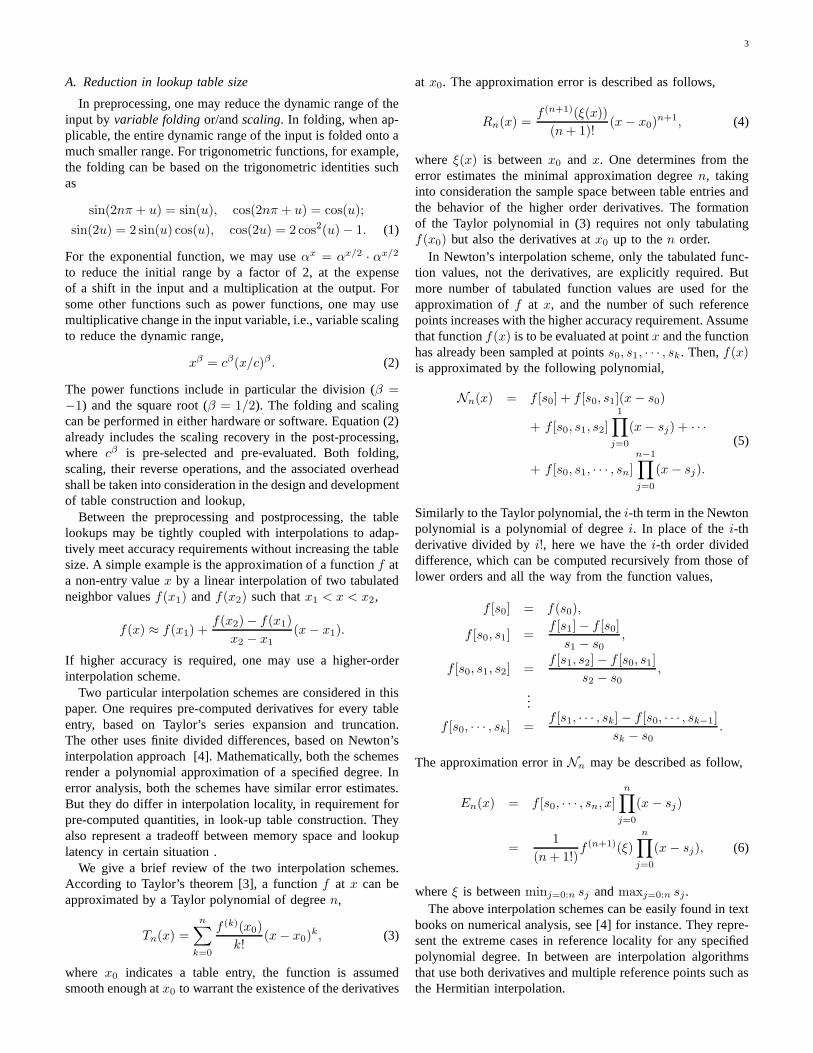
Fig. 1. Two sample clusters located in two sub-divided regions

In geometric tiling, we partition a matrix according to thegeometric locations of the sample data associated with thematrix. First we partition and cluster the samples based ona prescribed clustering rule. Imagine that all the particles,the sources and targets, are bounded in a box B. We mayassume that one of the box’s corners is at the origin, seeFigure 1. Specifically, one may subdivide the box B intoeight non-overlapping smaller boxes of equal size, B0, B1,B2, up to B7. Each and every particle falls into one of thesmaller boxes. Denote by Ti and Si the respective clustersof the target particles and source particles in box Bi. Thisparticle clustering scheme induces a virtual partition of theinteraction matrix into 8 × 8 tiles (sub-matrices). The (i, j)tile is K(Ti,Sj), the interaction matrix between clusters Ti

and Sj . This tile is empty if one of the clusters is empty.

5

−1

−0.5

0

0.5

1

1.5

2

2.5

3

3.5

4

−1

−0.5

0

0.5

1

1.5

2

2.5

3

3.5

4

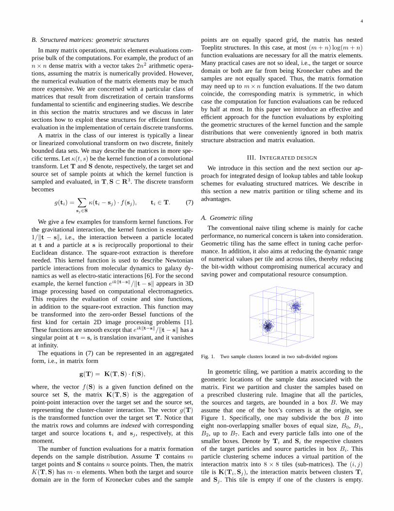
Fig. 2. Images of the interaction matrix associated with the two-clustersdatum set in a plain tiling (top) and in a geometric tiling (bottom) in logscale

For the case illustrated in Figure 1, the 8× 8 virtual partitionrenders a 2 × 2 partition of the interaction matrix with thezero partitions omitted. The corresponding matrix is shown inFigure 2.

We show in Figure 2 two images of the same interactionmatrix associated with the two-clusters datum set in Figure 1.The top image results from a plain tiling, oblivious to thegeometric information, and the bottom image from a geometrictiling. The numerical ranges in the partitioned tiles are indi-cated by colors. Any geometric tile may be further partitionedwith either geometric tiling or plain tiling, depending on thecircumstance of the integrated design.

Geometric clustering incurs an overhead. Fortunately, thisoverhead is linearly proportional to the total number of theparticles, which is smaller than the total number of theinteraction entries by an order of magnitude. Moreover, thisoverhead is subsumed by the many advantages of geometrictiling over plain tiling, as described in the next section.

B. Potential advantages

The impact of geometric tiling on efficient table lookupsmay be summarized as follows.

1. Reduction of dynamic range at the input of functionevaluation. Computing pairwise difference (t−s) and distance‖t − s‖ is common to the class of convolutional kernelfunctions we are interested in, as described in Section II-B. Within each geometric tile, the difference t − s betweenany source-target pair (t, s) in the same sub-box is less than,or at most equal to, half of the maximum particle-to-particledifference in the big box, in each and every component inmagnitude as well as in the Euclidean length. This reductionin the input range can be applied to all the translation-invariantkernel functions, in addition to folding or scaling wheneverapplicable.

By this fact the three coordinates of the difference t−s andthe distance ‖t− s‖ for each and every source-target pair in ageometric tile can be represented in hardware with one bit lesswithout compromising the numerical accuracy. Furthermore,one can refine the tiling to finer granularity, depending onthe sample distribution and the kernel function as well asarchitectural implementation complexity.

2. Reduction of dynamic range at the output of functionevaluation. The interaction functions considered here, suchas those examples given in Section II-B, are smooth. Basedon this property, a sufficiently refined geometric tiling canmake the numerical range of the source-target interaction overa tile smaller than or at most equal to half of the rangeover the whole matrix. For the gravitational interaction withκ(t, s) = 1/‖t− s‖, in particular, a partition of the box B inthe middle along each dimension is sufficient for this reductionin numerical range of the output over each and every geometrictile.

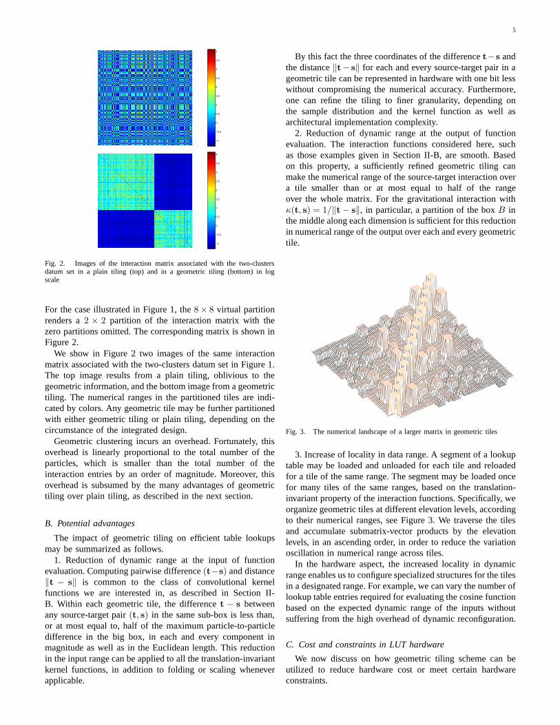
Fig. 3. The numerical landscape of a larger matrix in geometric tiles

3. Increase of locality in data range. A segment of a lookuptable may be loaded and unloaded for each tile and reloadedfor a tile of the same range. The segment may be loaded oncefor many tiles of the same ranges, based on the translation-invariant property of the interaction functions. Specifically, weorganize geometric tiles at different elevation levels, accordingto their numerical ranges, see Figure 3. We traverse the tilesand accumulate submatrix-vector products by the elevationlevels, in an ascending order, in order to reduce the variationoscillation in numerical range across tiles.

In the hardware aspect, the increased locality in dynamicrange enables us to configure specialized structures for the tilesin a designated range. For example, we can vary the number oflookup table entries required for evaluating the cosine functionbased on the expected dynamic range of the inputs withoutsuffering from the high overhead of dynamic reconfiguration.

C. Cost and constraints in LUT hardware

We now discuss on how geometric tiling scheme can beutilized to reduce hardware cost or meet certain hardwareconstraints.

6

Consider the situation where the memory for a LUT isvery limited. In this case, the numerical range of the inputparameters in successive cycles should be kept small. Thiscan be translated into an architectural constraint on geometrictiling at the algorithmic level. Integrating with the geometrictiling scheme, we can segment the entire range of the inputparameter into small ones that can meet the spatial constraintas well as the numerical accuracy requirement.

In Table I we illustrate with two simple segmentationoptions, the evaluation of the zero-order Bessel function J0

over a range of the input parameter ‖t− s‖ associated thesamples in the target set T and the source set S. The dynamicrange for the input in each segment in Design A is twice thatfor the design B. In other words, the table size for Design isas twice as that for Design B.

TABLE I

RANGE SEGMENTATION FOR FUNCTION J0

Design A: 5 segmentsInput Output

‖t − s‖ J0(‖t − s‖)[0, 2] [ 0.22, 1.00][2, 4] [ -0.40, 0.22][4, 6] [-0.40, 0.15][6, 8] [ 0.15, 0.30][8, 10] [ -0.25, 0.17]

Design B: 10 segmentsInput Output

‖t − s‖ J0(‖t − s‖)[0, 1] [ 0.77, 1.00][1, 2] [ 0.22, 0.77][2, 3] [-0.26, 0.22][3, 4] [-0.40, -0.26][4, 5] [-0.40, -0.18][5, 6] [-0.18, 0.15][6, 7] [ 0.15, 0.30][7, 8] [ 0.17, 0.30][8, 9] [-0.09, 0.17][9, 10] [-0.25, -0.09]

IV. HARDWARE-EFFICIENT INTERPOLATIONS

In this section, we introduce an approach to exploitingthe data locality provided by geometric tiling for hardware-efficient interpolations in combination with table lookups.We illustrate the approach in particular with the Newtoninterpolation approach as described in Section II-A.

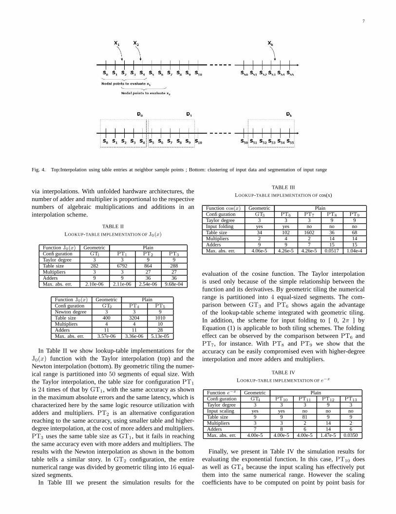
The use of the Newton interpolation method may be pic-torially described in Figure 4. The sample or nodal points,denoted by sp, are assumed equally spaced, although notnecessarily. The evaluation points at non-nodal locations aredenoted by xq . For a particular function and a specifiedevaluation accuracy, we determine based on the error estimatein (6) the number of nodal points for interpolation at anynon-nodal point x within the input range, which may bereduced as we have discussed. Suppose five nodal pointsgive sufficient accuracy. Then, the function evaluation at x1

needs table entries associated with the nearby sample pointss0, s1, s2, s3, s4, see the top of Figure 4. The evaluation at x2

needs table entries at s2, s3, s4, s5, s6.By utilizing the geometric tiling scheme, the input values for

function evaluations are clustered. In other words, the entiredynamic range of the input is divided into smaller sub-regions,which may or may not overlap. Some of the sub-regions areshown by the bounding intervals D0, D1, · · ·, Dk at the bottomof Figure 4. For all the evaluation points within the same sub-interval, the same segment of table entries can be used. Forexample, to compute f(x) for all x in D1, it is sufficient touse only the table entries at s5, s6, s7, s8, s9.

The higher order differences f [s0, s1, · · · , sk], where k ≤ 4by the above assumption, can be treated with two differentoptions. They can be pre-computed to minimize the interpo-lation latency. Or, they can be re-computed whenever needed,without increasing the table size quadratically relative to thetotal number of sample points. There is thus a memory-latencytradeoff. We point out that this frequent re-computation andincreased latency can be substantially reduced by functionevaluation on clustered input data. Specifically, the higherorder differences are computed only once for every inputcluster, used and re-used for the function evaluation at all theinput values in the cluster.

V. SIMULATION RESULTS

We present in this section primary simulation results todemonstrate the reduction in table size and other computationresources achieved by integrating geometric tiling with thedesign and use of lookup tables for extensive function evalua-tions in certain structured matrix computation as described inthe previous sections. The reduction is shown by comparingthe integrated scheme to the conventional scheme withoutgeometric clustering. To have fair comparisons, we let bothschemes meet the same prescribed accuracy requirement withminimal cost within each scheme.

We shall describe first the setup for the simulation results.Lookup tables and interpolations are simulated in MATLABwith single-precision floating arithmetic. We experiment withtwo elementary functions cos(x), e−x and one special functionJ0(x), the zero-order Bessel function of the first kind. Theinput folding and scaling scheme are applicable to the cosinefunction and exponential function, respectively, but not to theBessel function. The initial range for the input is specified as(0, 100) for the cosine and Bessel functions, and (0, 10) forthe exponential function. The sampling points for the tableentries are uniformly distributed.

We carry the interpolation experiments with the two meth-ods described in Section II-A. We alter the accuracy by varyingthe degree of the interpolation polynomials, see Equations(3) and (5). The errors in the interpolation are estimatedanalytically by (4) and (6), respectively, and further testednumerically. In numerical testing, the accuracy of functionevaluations is described by the worst deviation from that byMATLAB in double-precision floating-point arithmetic, whichwe refer to as the maximum absolute errors in the followingtables.

Next we present and explain the simulation results inTables II, III and IV. We use GT and PT to denote geometrictiling and plain tiling, respectively. Each individual configura-tion, labeled with either GT or PT with a subscript, is specifiedby the interpolation degree in a specified interpolation scheme,the size of lookup table, the number of adders and the numberof multipliers. The table size refers to the total number ofcoefficients in the terms in Equations (3) and (5). In hardwareimplementation such as using field programmable gate arrays,these coefficients can be pre-calculated and stored in desig-nated memory. Hardware resources also include the adders andmultipliers used for function evaluation at non-tabulated points

7

Fig. 4. Top:Interpolation using table entries at neighbor sample points ; Bottom: clustering of input data and segmentation of input range

via interpolations. With unfolded hardware architectures, thenumber of adder and multiplier is proportional to the respectivenumbers of algebraic multiplications and additions in aninterpolation scheme.

TABLE II

LOOKUP-TABLE IMPLEMENTATION OF J0(x)

Function J0(x) Geometric PlainConfiguration GT1 PT1 PT2 PT3

Taylor degree 3 3 9 9Table size 282 6792 864 288Multipliers 3 3 27 27Adders 9 9 36 36Max. abs. err. 2.10e-06 2.11e-06 2.54e-06 9.68e-04

Function J0(x) Geometric PlainConfiguration GT2 PT4 PT5

Newton degree 3 3 9Table size 400 3204 1010Multipliers 4 4 10Adders 11 11 28Max. abs. err. 3.57e-06 3.36e-06 5.13e-05

In Table II we show lookup-table implementations for theJ0(x) function with the Taylor interpolation (top) and theNewton interpolation (bottom). By geometric tiling the numer-ical range is partitioned into 50 segments of equal size. Withthe Taylor interpolation, the table size for configuration PT1

is 24 times of that by GT1, with the same accuracy as shownin the maximum absolute errors and the same latency, which ischaracterized here by the same logic resource utilization withadders and multipliers. PT2 is an alternative configurationreaching to the same accuracy, using smaller table and higher-degree interpolation, at the cost of more adders and multipliers.PT3 uses the same table size as GT1, but it fails in reachingthe same accuracy even with more adders and multipliers. Theresults with the Newton interpolation as shown in the bottomtable tells a similar story. In GT2 configuration, the entirenumerical range was divided by geometric tiling into 16 equal-sized segments.

In Table III we present the simulation results for the

TABLE III

LOOKUP-TABLE IMPLEMENTATION OF cos(x)

Function cos(x) Geometric PlainConfiguration GT3 PT6 PT7 PT8 PT9

Taylor degree 3 3 3 9 9Input folding yes yes no no noTable size 34 102 1602 36 68Multipliers 2 4 2 14 14Adders 9 9 7 15 15Max. abs. err. 4.06e-5 4.26e-5 4.26e-5 0.0517 1.04e-4

evaluation of the cosine function. The Taylor interpolationis used only because of the simple relationship between thefunction and its derivatives. By geometric tiling the numericalrange is partitioned into 4 equal-sized segments. The com-parison between GT3 and PT6 shows again the advantageof the lookup-table scheme integrated with geometric tiling.In addition, the scheme for input folding to [ 0, 2π ] byEquation (1) is applicable to both tiling schemes. The foldingeffect can be observed by the comparison between PT6 andPT7, for instance. With PT8 and PT9 we show that theaccuracy can be easily compromised even with higher-degreeinterpolation and more adders and multipliers.

TABLE IV

LOOKUP-TABLE IMPLEMENTATION OF e−x

Function e−x Geometric PlainConfiguration GT4 PT10 PT11 PT12 PT13

Taylor degree 3 3 3 9 3Input scaling yes yes no no noTable size 9 9 81 9 9Multipliers 3 3 2 14 2Adders 7 8 6 14 6Max. abs. err. 4.00e-5 4.00e-5 4.00e-5 1.47e-5 0.0350

Finally, we present in Table IV the simulation results forevaluating the exponential function. In this case, PT10 doesas well as GT4 because the input scaling has effectively putthem into the same numerical range. However the scalingcoefficients have to be computed on point by point basis for

8

PT10, while on tile by tile basis for GT4. The scaling effectis evident by the comparisons among PT10, PT11, PT12 andPT13.

VI. CONCLUSION

The hardware-efficient techniques introduced in this paperfor function evaluations associated with certain structured ma-trix computation are based on the principle concept of breakingdown or shifting the traditional boundaries and tradeoffs inalgorithmic module abstraction, architectural module abstrac-tion, and between algorithms and architectures. Specifically,the design and use of lookup tables as an efficient functionevaluation component are combined with and enhanced byalgorithmic techniques such as input folding, scaling andespecially geometric tiling, which is based on a new matrixabstraction to preserve the geometric information that is com-monly available but was neglected. A broader realization ofthis principle concept is on algorithm-architecture codesign ofspecial-purpose systems, [5] which may include one or morefunctions to be evaluated.

The experiments presented in Section V are intended todemonstrate the promise and impact of these integrationtechniques. There are many more architectural choices thanpresented, such as hardware configurations with folded struc-tures using fewer adders and multipliers. This may in turnchange the pipeline structure and the latency. This varietyin design options shows a great opportunity for performanceenhancement and optimization in the architectural designspace. As we have illustrated in this paper, it is not necessarilyhard to integrate architectural design and algorithmic design,and the payoff from such integration is substantial.

REFERENCES

[1] W. C. Chew. Waves and Field in Inhomogeneous Media. Van NostrandReinhold, New York, 1990.

[2] B. Parhami (editor). Computer arithmetic algorithms and hardwaredesigns. Oxford University Press, 2000.

[3] J.W. Hauser and C.N. Purdy. Approximating functions for embedded andasic applications. In Proceedings of the 44th IEEE Midwest Symposiumon Circuits and Systems, volume 1, pages 478–481, Aug 2001.

[4] F. B. Hildebrandt. Introduction to Numerical Analysis. McGraw-HillBook Company, 1956.

[5] J. Kim, P. Mangalagiri, M. Kandemir, V. Narayanan, L. Deng, K. Sobti,C. Chakrabarti, N. Pitsianis, and X. Sun. Algorithm-architecture codesignfor structured matrix operations on reconfigurable systems. TechnicalReport CS-2006-11, Department of Computer Science, Duke University,2006.

[6] B. Thide. Electromagnetic Field Theory. Upsilon Books, 1997.