1

Efficient Cyber Attack Detection in IndustrialControl Systems Using Lightweight Neural

Networks and PCAMoshe Kravchik and Asaf Shabtai

Abstract—Industrial control systems (ICSs) are widely usedand vital to industry and society. Their failure can have severeimpact on both economics and human life. Hence, these systemshave become an attractive target for attacks, both physicaland cyber. A number of attack detection methods have beenproposed, however they are characterized by a low detectionrate, a substantial false positive rate, or are system specific. Inthis paper, we study an attack detection method based on simpleand lightweight neural networks, namely, 1D convolutions andautoencoders. We apply these networks to both the time andfrequency domains of the collected data and discuss pros and consof each approach. We evaluate the suggested method on threepopular public datasets and achieve detection rates matching orexceeding previously published detection results, while featuringsmall footprint, short training and detection times, and generality.We also demonstrate the effectiveness of PCA, which, givenproper data preprocessing and feature selection, can provide highattack detection scores in many settings. Finally, we study theproposed method’s robustness against adversarial attacks, thatexploit inherent blind spots of neural networks to evade detectionwhile achieving their intended physical effect. Our results showthat the proposed method is robust to such evasion attacks: inorder to evade detection, the attacker is forced to sacrifice thedesired physical impact on the system. This finding suggests thatneural networks trained under the constraints of the laws ofphysics can be trusted more than networks trained under moreflexible conditions.

Index Terms—Anomaly detection; Industrial control systems;convolutional neural networks; autoencoders; frequency analysis;explainability; adversarial machine learning; adversarial robust-ness.

I. INTRODUCTION

Industrial control systems (ICSs), also known as supervisorycontrol and data acquisition (SCADA) systems, combinedistributed computing with physical process monitoring andcontrol. They are comprised of elements providing feedbackfrom the physical world (sensors), elements influencing it (actu-ators), as well as computers and controller networks that processthe feedback data and issue commands to the actuators. ManyICSs are safety-critical, and an attack interfering with theirfunctionality can cause substantial financial and environmentalharm, and endanger people’s lives.

The importance of ICSs makes them an attractive target forattacks, particularly cyber attacks. Several high impact incidentsof this kind have been reported in recent years, including theattack on a power grid in Ukraine [1], the infamous Stuxnet

The authors are with the Department of Software and Information SystemsEngineering, Ben-Gurion University of the Negev, Beer-Sheva, Israel. E-mail:moshekr@post.bgu.ac.il, shabtaia@bgu.ac.il.

malware that targeted nuclear centrifuges in Iran [2], and attackson a Saudi oil company [3]. In the past, ICSs ran on proprietaryhardware and software in physically secure locations, but morerecently they have adopted common information technology(IT) stack and remote connectivity. This trend exposes ICSsto cyber threats that leverage common technology stack attacktools. At the same time, the ICS defender’s toolbox is limiteddue to the need to support legacy protocols built withoutmodern security features, as well as the inadequate processingcapabilities of the endpoints. This problem can be addressedby utilizing traditional IT network-based intrusion detectionsystems (IDS) to identify malicious activity, which does notrely on endpoint computational resources. However, the verylow number of known attacks on ICSs renders this approachineffective. Alternatively, model-based methods have beenproposed to detect anomalous behavior of the monitoredICS [4]–[7]. Unfortunately, creating an accurate model ofcomplex physical processes is a very challenging task. Itrequires an in depth understanding of the system and itsimplementation, and is time consuming and difficult to scale.Thus, recent studies have utilized machine learning to modelthe system. Some of them used supervised learning [8], [9] andachieved high precision results, however the supervised learningapproach is limited to the modeled attacks only. To overcomethis obstacle, a number of other studies used unsupervised deepneural networks (DNNs) for detecting anomalies and attacksin ICS data [10]–[12]. Kravchik and Shabtai [13] suggestedusing unsupervised neural networks based on 1D CNNs anddemonstrated the detection of 31 out of 36 cyber attacks inthe popular SWaT dataset [14], improving upon previouslypublished results. This paper extends the research performedin [13] and is aimed at answering the following questions thatwere not addressed in that study.

• Can the generality and effectiveness of a 1D CNNbe validated using additional datasets, preferably fromdifferent types of system?

• Are there alternative lightweight neural network architec-tures that can be used in the method proposed in [13]?

• Can the detection of an anomaly be interpreted in sucha way that it provides actionable insights to the systemoperator, namely how to pinpoint the attacked sensors oractuators?

• Will detection in the frequency domain provide anybenefits compared to detection in the time domain?

• How robust are the proposed neural networks architectures

arX

iv:1

907.

0121

6v2

[cs

.CR

] 1

Oct

201

9

2

to adversarial machine learning attacks?The contributions of this paper are as follows.• An effective and generic method for detecting anomalies

and cyber attacks in ICS data using 1D CNNs andundercomplete autoencoders (UAEs). The method wasvalidated on three public datasets and achieved betterperformance than previously published research in thisarea.

• A method for robust feature selection based on theKolmogorov-Smirnov test.

• A method for attack detection explanation - attacklocalization using neural network-based models.

• The efficient application of the above mentioned detectionmethod to the frequency domain which provides highdetection scores and guidelines for when to use it.

• A demonstration of the adversarial robustness of theproposed method under a powerful white-box attackerthreat model.

The rest of this paper is organized as follows. In Section II,we present the necessary background on ICSs, the consideredthreat model, relevant neural network architectures, time-frequency transformation, and adversarial machine learning. InSection III, we survey related work, focusing on physical sys-tem state-based detection research. Section IV, introduces thedatasets we used for validation. We describe our methodologyin Section V. The experiments and their results are describedin Section VI, and finally, Section VII concludes the paper.

II. BACKGROUND

A. Industrial Control Systems

A typical ICS combines network-connected computerswith physical processes, which are both controlled by thesecomputers and provide the computers with feedback. The keycomponents of an ICS include sensors and actuators that areconnected to a local computing element, commonly called aprogrammable logic controller (PLC) or a remote terminal unit(RTU).

Sensors and actuators are usually connected to the PLCwith a direct cable connection, and commands are sent to thePLC via a local networking protocol, such as CAN, Profibus,DNP3, IEC 61850, IEC 62351, Modbus, or S7. PLCs of theremote nodes are connected to the central control unit viaprotocols, such as TCP, over a wireless, cellular, or wirednetwork. The connection is made with the help of a dataacquisition system (DAS) that bridges the local and remotenetworking protocols. The central control node contains amaster terminal unit (MTU) that applies the control logic tothe RTUs and provides management capabilities to a humanmachine interface (HMI) computer. A historian server thatcollects and stores data from the RTUs is another importantICS component. An additional common element of ICSs is anengineering workstation running SCADA software that providesa means to both monitor the PLCs and to change their internallogic.

Recently, many SCADA and PLC components startedsupporting the Common Industrial Protocol (CIP), which allowsthe integration of industrial control applications with a standard

network stack. Using SCADA and PLC components supportingsuch modern protocols enables system simplification, allowingthe removal of dedicated MTU and DAS components.

B. Attacks on ICSs and Threat Model

The central role of ICSs in critical infrastructure, medicaldevices, transport, and other areas of society makes them anattractive target for attacks. Motives for such attacks are diverseand include criminals seeking control of an important assetor blackmailing a victim, industrial espionage and sabotage,political reconnaissance, cyber war, and privacy evasion.

An ICS can be attacked using several attack vectors includingsoftware, hardware, communication protocols, the physicalenvironment, and human elements.

For example, an adversary can attack:1) The HMI machine, by exploiting software vulnerabilities

in its OS and application stack, presenting a fake view ofthe process and causing the operator to issue erroneouscommands [15],

2) The SCADA and/or engineering workstation machine,by exploiting software vulnerabilities and obtaining fullcontrol of the ICS, as it happened in Ukraine [1],

3) The communication network in the control segment, inthe remote segment, or between them, by performingeavesdropping, or replay or false packet injection attacks,

4) The PLC, by exploiting software vulnerabilities or trustbetween the PLC and SCADA; this will allow the attackerto change the PLC logic influencing the controlledprocess and cause damage, as in the Stuxnet case,

Fig. 1. A schematic of ICS architecture and possible attack locations on anICS system.

3

5) The sensors, by leveraging physical effects interferingwith the measurement or replacing the sensor with amalicious one as shown in [16], or,

6) The actuators, by altering the signal sent by the actuatorsto the controlled process, as described in [17].

The attack can also combine a number of vectors, forexample issuing malicious commands to the actuator andreplaying a valid system state to the SCADA, as done bythe Stuxnet malware. Figure 1 illustrates most common attacklocations.

Our threat model considers a powerful adversary that is ableto influence the physical state of the protected ICS. Regardlessof the attack vector, the most common ultimate goal of theattacker is a physical-level process change. Hence, in thisresearch, we don’t assume any specific attack vector, and applya physics-based attack detection approach. The main idea ofthis approach is that the behavior of the protected systemcomplies with immutable laws of physics and therefore can bemodeled. Monitoring the physical system state and its deviationfrom the model facilitates the detection of anomalous behavior,including the deviations caused by spoofed sensor readingsand injected control commands. For example, opening a valveshould result in an increase in the water level. If the level doesnot increase or the speed of the increase is higher than usual,the sensor reading could have been falsified, or the sensormight be faulty.

Despite the fact that our anomaly detection domain ispurely physical, we argue that our method goes beyondsimple anomaly detection. As we show, it can detect sophis-ticated multi-point cyber attacks that combine data tampering,malicious commands and replay attacks. These attacks aretargeted, evasive, and performed by means of the cyber domain.Therefore, we choose to classify the method as cyber attackdetection. Adding the cyber context to our detection domain,e.g., by combining network and sensory data, is a promisingdirection for future research. As the network data was notavailable in most of the public datasets, we made the decisionto focus on physical-only detection in this research.

C. Convolutional Neural Networks

Convolutional neural networks (CNN) are feedforward neuralnetworks popular in image processing domain. In the basicneural network model, the layers are fully connected, whichmeans that a unit (a neuron) is connected to all of the units inthe subsequent layer. This requires the neuron to hold a verylarge number of weights on these connections. This structuredoes not scale well, and such a large number of parameters(weights) will usually lead to overfitting. In addition, fullyconnected networks ignore the input topology: input variablescan be presented in any order, and the outcome will be the same.However, many kinds of data, including images, have a distinctstructure, and nearby pixels are highly correlated. CNNs addressthese deficiencies by applying convolutions (filters) to smallregions of the input instead of performing matrix multiplicationon all of the input at once. The filter uses the same weightsfor all of the locations and thus can detect features regardlessof their position in the image. A convolutional layer consists

Fig. 2. Denoising Autoencoder.

of several feature maps each detecting a different input feature.1D CNNs can successfully be used for time series processing,because time series have distinct 1D (time) locality that canbe extracted by convolutions [18].

D. Autoencoders

An autoencoder (AE) is a neural network trained to reproduceits input [19], thereby learning useful properties of the data.This is achieved by applying constraints on the networkwhich prevent copying the input to the output and cause thenetwork to learn the compact representation of the data. Dueto this ability, autoencoders are widely used for dimensionalityreduction and feature learning [19]. Autoencoders have twomajor components: an encoder that transforms the input intosome internal representation, and a decoder that reconstructs theinput from this representation. The simplest kind of autoencoderis an undercomplete autoencoder (UAE), which passes the datathrough a bottleneck of a hidden layer with smaller dimensionsthan the input and output. This bottleneck forces the networkto learn a subspace which captures principal features of thedata. Another way of forcing an autoencoder to learn importantinput structural features is letting it reconstruct the originalinput from the input after it has been corrupted by noise. Acommon way to corrupt the input is to add some Gaussiannoise to it. Autoencoders that utilize this technique are calleddenoising autoencoders (DAEs) (see Figure 2).

Variational autoencoders (VAE) [20] have become verypopular in the unsupervised learning of complex distributionsand in generating images of different kinds. While regularautoencoders learn a compact representation of the input data,there is no constraint on this compact representation. Forexample, given an autoencoder network trained with manyimages of dogs, we still don’t know how to build an internalrepresentation that could generate a dog when passed tothe decoder part of the network. VAE solves this problemby applying constraints on the distribution of the compactrepresentation (called a latent variable or code). To impose thisconstraint, the loss function is a sum of the data reconstructionerror (generalization error) and a deviation of the latent variabledistribution from some chosen prior distribution, typically aunit Gaussian distribution. Once the network is trained, it ispossible to generate new images of dogs by drawing samplesfrom the unit Gaussian distribution and passing them to thedecoder. A VAE has three parts: an encoder, decoder, and priordistribution (as illustrated in Figure 3). The encoder creates adistribution of the latent variables for the given input, and the

4

Fig. 3. Variational Autoencoder.

decoder returns a distribution of inputs corresponding to thegiven latent variables. The network is trained to maximize thelikelihood of the data given the codes it assigns to it, whilemaintaining the codes’ distribution close to the chosen priorone.

E. Time - Frequency Domain Transformation

Raw data measured by ICS sensors produces a time series.While in most ICS anomaly and attack detection researchthis data is processed directly, it is very common in signalprocessing to analyze data in the frequency domain. Fouriertransform (1) allows us to build a signal’s frequency domainrepresentation:

f(k) =

∫ +∞

−∞f(x)e−2πixkdx, (1)

where f is some function depending on time x, f is its Fouriertransform, and k is the frequency. When dealing with periodicdata samples, rather than a continuous function, the discreteFourier transform is used:

Fk =

N−1∑n=0

fne−2πink/N , (2)

where fn denotes the n-th sample of f . Fourier transformof a time series provides its spectrum over the entire periodof time measured. In order to detect changes in the signalspectrum over time, the short-time Fourier transform (STFT) isused. STFT applies the Fourier transform to short overlappingsegments of the time series.

Frequency domain analysis provides several advantages. First,it provides a more compact and concise representation of mostof the dominant signal components. Second, it allows for thedetection of attacks involving changing the frequency of regularoperation modes, e.g., quickly starting and stopping the engine.Lastly, according to the uncertainty principle [21], functionslocalized in the time domain (e.g., a short spike) are spreadacross many frequencies, and functions that are concentratedin the frequency domain are spread across the time domain.This means that slow attacks that usually evade time domaindetection methods will stand out in frequency analysis, butshort attacks will be difficult to detect using it.

F. Adversarial Attacks on Machine Learning Models

In this section, we provide a brief overview of adversarialattacks. A more complete review of related work in the contextof this research is presented in Section III. Adversarial datais specially crafted input samples that cause the algorithm toproduce incorrect results at test time. The field of adversarial

learning in DNNs has gained a lot of interest since [22]showed that neural network-based classifiers can be trickedinto mislabeling an image by changing a small number ofpixels in a way that is imperceptible to the human eye. Sincethen, successful adversarial attacks on neural networks havebeen demonstrated in malware detection, speech classification,and other areas.

Adversarial machine learning attacks can be divided intopoisoning attacks performed at training time and evasionattacks performed at test time. In order to model adversarialattacks, we need to consider the attacker’s goals and knowledge.According to [23], the goals are further subdivided intothe desired violation (integrity, availability, or privacy) andspecificity (targeting a set of inputs or all of them, as wellas producing specific output or just any incorrect output). Inthe context of anomaly detection, the attacker’s goal mightbe to cause the system to classify an anomaly as benign(specific integrity attack) or to classify many benign samplesas anomalous to decrease the trust in the detection results(indiscriminate availability attack).

Bigglio et al. [23] define the attacker’s knowledge in termsof the training data D, the feature set X , the algorithm fand its objective function L, the training hyperparameters,and the detection parameters w learned. In the context of ourresearch, X is the set of sensors’ and actuators’ states used totrain the model, while f and L represent the selected neuralnetwork architecture and its loss function. Thus, the attacker’sknowledge is represented by the components (D,X , f, w). Theworst-case perfect knowledge white-box scenario happens whenall four components are known. Gray-box attacks occur if atleast one of the components is not known and cannot bereproduced. For example, the attacker might know the featureset and the neural network type, but the network parametersand weights are not known. In such cases, the attacker tries tocreate a surrogate model using training data sets relevant to theproblem and transfers the attack created on the surrogate modelonto the real one. Black-box attacks are characterized by thelack of specific knowledge about any of the four components.The attacker, however, knows that some model is used for thetask at hand and can make educated guesses about the kind offeatures it uses to solve it.

III. RELATED WORK

The area of anomaly and intrusion detection in ICSs hasbeen widely studied. Extensive surveys [24]–[26] and surveysof surveys [27] are devoted to the classification of researchin this field. In our review of related work, we focus on ICSanomalies and cyber attack detection using the physical stateof the system as measured by the sensors. As noted in [17], thefirst step in physics-based detection is system state prediction.By observing the deviation between the predicted and reportedsystem state, a decision is made on whether an attack oranomaly occurred and how to score it. Hence, one of the mainways to classify the research is by the prediction method used.Auto-regressive (AR) models are used to predict the systemstate in [28] and [29]. While popular in time series analysis,these models have limitations in multivariate systems, when

5

the state of one observed variable is correlated with another. Inour research, we use DNNs that don’t have these limitations.

Another popular way of modeling the system is rooted inthe control theory and uses the subsystem model identificationbased on equation (3) which describes a linear dynamicalsystem:

xk+1 = Axk +Buk + εkyk = Cxk +Duk + ek,

(3)

where xk is the system state at time k, uk denotes the controllercommands to actuators, yk are the sensor measurements, εkis perturbation noise, ek is sensor noise, and A,B,C,Dare matrices modeling the dynamics of the system. Thisapproach has been used in previous studies, such as [30]–[32]. The limitations of linear dynamical system modelinginclude the requirement for controller command measurement,a requirement which is not met in most datasets. In addition,many attack scenarios involve altering PLC logic and do notviolate system dynamics. For those reasons, we chose to useDNNs that are more flexible on both counts.

Specification-based system modeling can also be veryeffective, as shown by [33] and [7]. In [33], the authors usedbehavior rules to specify the safe system state for medicalCyber Physical Systems (CPSs) and monitor deviation fromthese rules. Distributed invariant-based mechanisms for smartgrids are presented in [34] and [35]. In [35], detection isbased on observing the physical state of the shared system,detecting the power conservation invariants’ violation andidentifying the rogue component by the invariants’ verificationin its topological neighborhood. While effective in rogueCPS controller identification, the solution proposed in [35]is very specific to smart grids, where the physical invariantsare well-known and simple. Rahman et al. [34] used multiplecomputationally powerful agents that communicated with eachother. One of the main drawbacks of these approaches is theirspecificity - the solution should be tailored to the system andits operating conditions; in contrast, our approach is genericand requires no manual configuration.

PASAD is a novel approach to the problem presented in[36]. PASAD is based on ideas from singular spectrum analysisand detects attacks in the signal subspace representing thedeterministic part of the time series. The main idea of PASADis to break the signal into subseries and find their noise-reducedrepresentation by singular value decomposition. The principledifference between our detection approach and PASAD is theability of our approach to detect anomalies in correlation amonginput features, while PASAD is limited to a single time series.

In a recent competition on water distribution system cyberattack detection (the BATADAL - BATtle of the AttackDetection Algorithms [37]), seven teams demonstrated theirsolutions on a simulated dataset. The best results were shownby the authors of [38], who were able to model the systemprecisely using MATLAB. The main limitation of this solutionis its reliance on the need and ability to create a precisesystem model, both a non-generic and difficult task. Anotherwork that achieved a high score in the competition is [39] inwhich the authors proposed a three-layer method, where thefirst layer detects statistical anomalies, the second layer is a

neural network aimed at finding contextual inconsistencies withnormal operation, and the third layer uses principal componentanalysis (PCA) on all sensor data to classify the samplesas normal or abnormal. Our work differs from [39] in thefollowing ways. First, we study the efficiency of a singlegeneric mechanism, as opposed to the multilevel system usedby [39]. Second, our solution evaluates types of neural networksnot covered by [39]. In addition, we study frequency domainanomaly detection and adversarial robustness.

Another relevant study from the BATADAL competitionis [40]. In addition to other detection mechanisms, the authorsof [40] used VAEs to calculate the reconstruction probabilityof the data. In our research, we found that VAEs are notvery accurate in reconstructing time series data. Therefore, wesuggest using simpler autoencoder models and demonstratetheir effectiveness at this task.

Neural networks have been used in additional physics-basedcyber attack detection research ( [10]–[12]). Unlike our work,these studies use more complex recurrent and graphical modelsand do not study the frequency domain.

Autoencoders have been used for anomaly and intrusiondetection before [41], [42]. The differences between this workand [41] are that in our research (1) AEs are applied to rawphysical signals without statistical feature extraction, and (2)AEs are applied to the frequency domain. We extend theresearch in [42] by applying AEs to cyber attack detection intime series, combining control, status and raw physical data,as well as applying AEs to the frequency domain. We alsoenhance the architecture of the network and present a featureselection method which improves network performance.

After our research was complete we discovered a recentpublication by Taormina et al. that applied autoencoders tothe BATADAL dataset [43]. The authors demonstrated theeffectiveness of AEs and were able to achieve an F1 scoreof 0.886. Also, the authors showed how to obtain insight onthe attack location from the model’s predictions. Our researchwas performed in parallel to [43], was not influenced by itsfindings, and differs from it in the following ways:• we study both 1D CNNs and AEs on three different

datasets, two of which come from real-world testbeds,• our AE architecture is different because it has been

adopted to multivariate time series prediction, uses noiseand an inflation layer; it also achieves a higher F1 score,

• we study frequency domain detection, and• we present adversarial attacks on the proposed network

and its robustness.Little attention has been given to adversarial attacks in the

ICS context, and there are a number of differences betweenour study and the work in the area where most of adversarialresearch has been done (image and sound processing):• most of the existing work is focused on supervised learning

problems, while our research deals with a semi-supervisedlearning,

• most of the existing work is focused on classification tasks,while in our research we deal with prediction (regression),

• while in tasks such as image classification the outputvariable (picture class) is not part of the input, in our taskthe input and output features are same, and

6

• in our case, there are multiple constraints on the internalstructure of the data, due to the laws of physics and PLClogic, that are not present in images.

A successful evasion attack framework on machine learninganomaly detection was demonstrated in [44]. The authors wereable to bring a monitored reactor to a dangerous pressurelevel by manipulating sensor measurements in a way that wasclassified by both a linear regression and a feed-forward neuralnetwork as normal. In [45], the authors used a GAN (generativeadversarial network) in order to create stealthy attacks on anICS, evading a baseline anomaly detector. Most recently, Erbaet al. [46] showed how to create successful evasion attacksagainst an autoencoders-based detection mechanism. The maindifference of [46] and our approach is the threat model chosen.The authors of [46] consider a very powerful attacker that canboth generate arbitrary malicious inputs to the PLC and createfake traffic that is fed to the detector. We consider a moreconstrained attacker that can only control the sensory data thatis both seen by the PLC and the detector. We argue that ourthreat model represents a more realistic scenario.

IV. DATASETS

A. SWaT

The Secure Water Treatment (SWaT) testbed was built atthe Singapore University of Technology and Design. Althougha detailed description of the testbed and dataset can be foundin [14], we provide a brief description below. The testbed is a

Fig. 4. SWaT testbed process overview [14].

scaled-down fully operational water treatment plant. As shownin Figure 4, the water goes through a six-stage process. Eachstage is equipped with a number of sensors and actuators.The sensors include flow meters, water level meters, andconductivity and acidity analyzers. Water pumps, chemicaldosing pumps, and valves that control inflow are the actuators.The sensors and actuators of each stage are connected to thecorresponding PLC, and the PLCs are connected to the SCADAsystem.

The dataset contains seven days of recording under normalconditions and four days during which 36 attacks wereconducted. The entire dataset contains 946,722 records, labeledas either attack or normal, with 51 attributes correspondingto the sensor and actuator data. The threat model used in

Fig. 5. Attack 30 on the LIT101 sensor. LIT101 measures the water levelin the first tank. P101 pumps the water out of the tank to the second stageprocessing. Note that after the attack is over, it takes a long time until thesystem returns to its normal production cycle.

the experiment is a system that has already been infected byattackers who spoof the system state to the PLCs causingerroneous commands to be issued to the actuators, or overridethe PLC commands with malicious ones. A table containing adescription and the timing of the attacks is provided in [14].Each attack aims to achieve some physical effect on the system.For example, attack 30 aims to cause underflow in the tank ofthe first stage. For that purpose, the value of the water levelsensor LIT101 is fixed at 700mm, while pump P101, whichcontrols water outflow is kept open for 20 minutes. Figure 5presents the attack, its effects, and the time it takes the systemto stabilize. The attacks were usually not stealthy, i.e., when acommand was issued to the actuator and the actuator changedthe system state, the change was not hidden by the attackers.

B. BATADAL

The BATADAL dataset represents a water distributionnetwork comprised of seven storage tanks with eleven pumpsand five valves, controlled by nine PLCs (see Figure 6). Thenetwork was generated with epanetCPA [47], a MATLABtoolbox that allows for the injection of cyber attacks andsimulates the response of the network to these attacks.

There are 43 variables representing the water tank levels,the flow and status of all of the pumps, as well as the inlet and

Fig. 6. Hierarchy of the water distribution system used in the BATADALdataset [48].

7

Fig. 7. Attack 12 on the L T2 sensor.

pressure for the pumping stations and valves. The training datasimulates hourly measurements collected for 365 days, resultingin 8,761 records. The test dataset contains 2,089 records (from87 days of recording). There are seven attacks present in the testdata. The attacks involved malicious actuator activation, PLCset point changes, and sensor measurement manipulation. Inaddition, the attacks were concealed from the SCADA systemby replacing the PLC-to-SCADA communication data withthe data recorded at the same hour during normal operation.Figure 7 illustrates attack 12. The goal of this attack is to causetank T2 to overflow. The L T2 sensor’s readings are alteredto report lower levels and cause PLC3 to keep the valve V2open. At the same time, the traffic from PLC3 to SCADA ismodified to replay previously recorded values of L T2, as wellas V2 flow and pressures. Figure 7 shows that the status of thevalve was not replayed, although the authors of [37] reportedthat it was. Also, one can see that immediately after the attackthe system returns to its regular cycle. This looks unrealistic,as the tank must be in an overflow state and it should taketime to process the excess water it contains. We estimate thatthese represent limitations of the simulation.

C. WADI

Finding another high-quality real-world cyber physicaldataset containing attacks is not an easy task. The best candidatewe could find is WADI [49], collected from a scaled-downwater distribution testbed and built by the authors of SWaT.The testbed consists of a number of large water tanks thatsupply water to consumer tanks. The dataset contains 16 attackswhose goal is to stop the water supply to the consumer tanks.The attacks were conducted by opening valves and spoofingsensor readings, and were partially concealed. The dataset issignificantly larger than the SWaT and BATADAL datasets,and contains 1,209,610 data points in the training set and 126features. The WADI dataset was made public recently, andvery few attack detection results utilizing this dataset havebeen published. In [7], the authors proposed an agent-basedframework for CPS modeling and used it to detect attackson the WADI dataset. Unfortunately, the authors of [7] did

not publish the quantitative metrics of the detection results,only reporting that 12 of 16 attacks were detected. In [50],the authors use LSTM-based generative adversarial networks(referred to as MAD-GANs in the paper) and show that theyoutperform other methods, such as PCA, K-nearest neighbors(KNN), and feature bagging (FB) on the SWaT and WADIdatasets.

V. METHODOLOGY

A. Data Analysis and Preprocessing

Our detection mechanism is based upon the ability to modeland predict the system’s behavior. To fulfill this requirement,the following assumptions must hold: the training data must berepresentative of the test data. More specifically, the trainingdata should contain all of the (latent) states, and the transitionsbetween them that appear in the test data. In other time-seriesforecasting techniques, e.g., AR models and recurrent neuralnetworks, there is a stronger requirement that the data needsto be stationary (i.e., maintains its probability distribution overtime) or can be transformed into stationary [19] form. Wefound that a number of SWaT features do not have the samedistribution in the training and test data (see Figure 8). In orderto obtain a quantitative measure of the similarity between theprobability distributions of the training and test data, we usedthe Kolmogorov-Smirnov test (K-S test) [51]. We chose theK-S test, because it is non-parametric and isn’t based on anyassumptions on the probability distributions tested. It also ismore sensitive than comparing the mean and standard deviationor the t-test, both of which do not work well with multimodaland non-normal distributions.

The K-S test statistic for two distributions is the maximaldifference between their empirical cumulative distributionfunctions (ECDF):

K-S = supx|F1(x)− F2(x)| , (4)

where F1 and F2 are ECDFs of the compared distributions.They can be found as:

Fx =1

n

n∑i=1

I[−∞,x](Xi), (5)

where

I[−∞,x] =

{1, if Xi < x

0, otherwise.

The original K-S test is limited to fully specified distributions[52], however we found the slight modification described belowuseful as a concise metrics for filtering out features unsuitablefor modeling. Using the maximum as a statistic makes theK-S test extremely sensitive to small CDF differences whenthe distribution’s mean is slightly offset on the x axis. Toincrease the test’s robustness, we used the area between theCDFs instead, which is calculated as:

K-S∗ =

∫x

|F1(x)− F2(x)| dx. (6)

Figure 8 illustrates three SWaT features, their values over time,histograms, and K-S and K-S* statistics.

8

We calculated the K-S∗ statistic for all SWaT andBATADAL features. The features were normalized to (0,1)scale. As Figure 9 shows, many of the SWaT features differgreatly between the training and test sets. Such features wouldcreate a lot of false positive alarms and must be excluded fromthe modeling. In addition to data normalization and featurestatistic profiling, we subsampled the SWaT data at a fivesecond rate. Subsampling provides a regularization mechanismwhich prevents overfitting and allows us to operate with asmaller amount of data.

As for the BATADAL dataset, all but one (P J280) of itsfeatures have very low K-S* metrics (10 or less). This strikingdifference between the real-world and simulated data stressesthe need to validate any findings in realistic setups.

For the WADI dataset, subsampling at a ten second rate wasapplied, and twelve unstable features were removed.

The feature selection step should be done prior to modeltraining, hence requiring different treatment for different data

Fig. 8. Feature statistic comparison. LIT101 has a very similar distributionin both the training and test data. AIT401 has a similar but slightly offsetdistribution. K-S has a high value, but K-S* correctly classifies the distributionsas close. AIT201 has very different distributions.

Fig. 9. K-S∗ statistic for the SWAT dataset. A number of features differsignificantly between the training and test sets.

availability scenarios:• if both training and test datasets are provided, the selection

should be done based on both of them,• if only the training dataset is available, the test can be

done on two parts of it, e.g., comparing the statistics ofthe first half of the data to the second, and

• a periodic validation of the features’ consistency can beperformed during the test period, and the model shouldbe retrained if significant changes are detected.

B. Undercomplete Autoencoders Design

After experimenting with multiple AE architectures, includ-ing LSTM-based AEs, variational AEs, and denoising AEs, wediscovered that the best detection performance is achieved withthe simplest undercomplete AEs. We describe the selected AEarchitecture here, and a comparison of the results in providedin Section VI-B.

The best results were achieved using the AE network variantadapted for multivariate sequence reconstruction. The networkdesign is as follows:• an optional corruption layer applying Gaussian noise to

the input sequence,• a fully connected layer with an ReLU or tanh activation

function inflating the input; the purpose of this layer isto enlarge the hypothesis space,

• an encoding layer that flattens the input and produces itscompact representation using a fraction of the input size;in our experiments the best results were achieved usingthe compact representation twice smaller than the input,

• a decoding layer reconstructing the original sequence fromits compact representation.

This architecture can deal with time sequences of arbitrarylength and is presented in Figure 10. We conducted a compari-son between the detection performance of a loss function basedon the reconstruction error for the predicted data points onlyversus the reconstruction error for the entire sequence. Thelatter produced much better results as illustrated in Figure 11.

C. Principal Component Analysis

Principal component analysis (PCA) transforms a set ofvariables to a set of values of linearly uncorrelated variables,orthogonal to each other. The new variables are linear com-binations of the original ones. PCA is based on eigenvectoranalysis and is often used for reducing the dimensions of thedata to a small number of principal components that representthe data’s internal structure in the way best explaining the datavariance. We used PCA as a baseline algorithm to comparethe performance of the neural networks. The use of PCA foranomaly detection in ICS is not new; it was suggested as oneof the detection layers in [39], and [42] used it for detectinganomalies in a simulated Lorenz system and telemetry data.In [39], detection was conducted in principal componentssubspace. Anomalies found in this subspace do not have adirect physical meaning in the original data feature space, andare hard to interpret and explain.

In our research, we used the approach outlined in Algorithm1. Our analysis restores the prediction to the original feature

9

Fig. 10. Autoencoders architecture used in this research.

Fig. 11. Improvement of detection score when measuring loss for the entiresequence in autoencoders.

space thus allowing for the natural application of the detectionand explanation method we use for neural networks, asdescribed below. To distinguish this detection method fromdetection in the principal components’ subspace, we refer toit as PCA-Reconstruction in Section VI. We implemented anextension to the classic PCA analysis. PCA usually operates onsingle time step vectors. This allows for the detection of contextinconsistencies between multiple features but is less powerful

Algorithm 1 Predict xtest given training data xtrain and usingPCA.

1: function PCAANALYSIS(xtrain, xtest, components)2: pcaModel← PCA(components)3: pcaModel.fit(xtrain)4: xtestPCA← pcaModel.transform(xtest)5: xtest ← pcaModel.inverse transform(xtestPCA))6: return xtest

in the detection of time-related inconsistencies in a singlefeature. To compensate for this deficiency, we implementeda windowed-PCA algorithm, which breaks the data into timewindows of a given width, performs the analysis depicted inAlgorithm 1 on vectors containing multiple data points, andthen restores the window predictions into the original signalshape. We later discovered that this idea was described in[53], where it is called Dynamical PCA. Two variants of thiswindowed-PCA algorithm were implemented: with overlappingand non-overlapping windows. The standard PCA algorithmimplementation from the Python scikit-learn package with thenumber of components equal to half of the modeled featureswas used as a basis for our experiments.

D. Frequency Domain Transformation

In order to explore the usefulness of frequency domain attackdetection we first had to transform the signals from the timedomain to the frequency domain. The following method wasused to create signal representation in the frequency domain(outlined in Algorithm 2 and illustrated in Figure 12).

1) Determine the dominant frequency of each signal (thefrequency with the most energy) using the discrete fastFourier transform (DFFT)(function frequencyAnalysis,lines 1-12).

2) Determine the window for the short-time Fourier trans-form (STFT) based on the dominant frequency period.It was found that the optimal window is between oneand two periods of the dominant frequency (line 16).

3) Transform the signals into their frequency representation.a) Split the entire signal into overlapping windows.b) Perform STFT for each window (these two items

are presented by the call to spectrogram at line 17).c) Binarize the entire spectrum of STFT into a number

of bins. Calculate the total energy of the signal ineach bin.

d) Pick a small number of bins with the most energy(lines 18-22). The energy values will represent thefeature in the frequency domain for the correspond-ing time window. We found that two or three bins

10

were sufficient for representing the features. It isalso possible to calculate the number of bins basedon the ratio of the total energy they contain (e.g.,at least 90%).

4) Apply the chosen neural network model (1D CNN orAE) to the frequency domain representation. As eachfeature is represented separately, the ability to locate theattack is maintained.

E. Adversarial Threat Model and Robustness Analysis

As this research was the first study of the proposed detectionmethod’s robustness to adversarial attacks, we assumed theworst-case scenario - a white-box attacker that knows every-thing about the model used for the detection, including itsweights. We consider an attacker that is trying to performa specific integrity attack, namely to cause a physical levelchange in the system’s behavior while staying undetected bythe monitoring anomaly detection system; the attacker caninfluence the values of sensors sent to the PLC but does nothave complete control of the network, in either the remote orthe control segment. Such an attack scenario is very common,especially in ICSs with sensors distributed over a large area andthat send their data to a PLC residing in a physically protectedand monitored center. In this setup, an adversary can replace

Algorithm 2 Transform signal s into frequency domainrepresentation

1: function FREQUENCYANALYSIS(s, sampling period) .Find the dominant frequency of the signal and its period

2: N ← len(s)3: freq ← DFFT (s) . The discrete FFT of the signal4: magn← abs(freq)[: N//2] ∗ 1/N . The magnitudes

of the real part of the FFT5: freq magn← listOf(freq,magn)6: sorted freq ← decreasedOrderSort(freq magn)7: if sorted freq[0][0] then . Ignore the constant

component if it has the most energy8: fundamental freq ← sorted freq[0][0]9: else

10: fundamental freq ← sorted freq[1][0]

11: period← (1.0/fundamental freq)/sampling period12: return (fundamental freq, period)

13: function FREQUENCYTRANS-FORM(s, rate, ratio, b num). Represent signal as energyin the most dominant frequency bands.

14: all freq bins← 1015: (f freq, period)← frequencyAnalysis(s, rate)16: STFT window ← period ∗ ratio17: freqs, Sx← spectrogram(s, rate, STFT window)18: bands← linspace(0, len(freqs), all freq bins+1)19: for i = 0 to all freq bins do20: bands energyi ←

∑bandsi+1

i=bandsiSxi

21: dominant bands ←decreasedOrderSort(bands energy)[: b num]

22: return dominant bands

Fig. 12. Frequency transformation of the L T1 feature. The first row depictsthe raw signal. The second row represents the STFT spectrogram on the leftand the power density distribution in the spectrum bands on the right. Thelast two rows are the frequency domain features - the power density in thefirst two bands.

the original sensor with a malicious one, reprogram the sensor,change its calibration, influence the sensor externally, or justsend false data to the PLC over the cable/wireless connection.We argue that this setup is much more practical than an attackercontrolling the internal network of the remote segment or eventhe network of the control segment, the scenario studied in[46]. In our threat model the attacker’s input is processed byboth the PLC and the detection system, hence the attacker’sgoal is to produce the input that will at the same time:

1) cause the intended physical impact on the system, and2) be close enough to the prediction of the detector to stay

under the detection threshold.Other characteristics of our threat model include:• the attacker can change multiple sensors,• the attacker can prepare the attacks offline; we argue

that if the system is characterized by periodic behavior,the attacker can choose the moment of the attack andprecompute the system state in our perfect knowledgethreat model, and

• the values of the sensors after the attack should be withinor close to the valid range of the sensor values (e.g. anon/off sensor can’t accept any other value).

As we did not possess access to the testbeds, we based ourstudy on adversarial manipulation of the SWaT dataset attacks.While this method cannot replace testing with a real system,it can provide an approximation of the ability to produce thedesired adversarial inputs. The two main limitations of suchdata-only research are:

1) it is limited to the attacks already present in the data set;even if none of them can’t be concealed by an adversarial

11

input there may be other attacks that have this capability,2) there is no way of testing the physical effect of an

adversarial sample found analytically on the real system.The adversarial robustness study was conducted as follows.

First, eighteen attacks from the SWaT dataset caused by spoofedsensors were selected. For each attack we performed gradient-based search for the adversarial input as outlined in Algorithm 3.This algorithm is adapted to a sequence prediction model thatprocesses the input using subsequences of length l, which weassume is also known to the attacker.

Algorithm 3 Find xadv given a trained model M, test datawith attack xatt, sub-sequence length l, a detection thresholdτ , acceptable noise level ε, input constraints φ.

1: function FINDSUBSEQADVINPUT(M, xatt, l, τ , ε, φ)2: M′ ←M+∇xJ(θ, x, y) . Add to the model graph

the cost function gradient calculation J given the modelparameters θ, input x and correct output y with respect tothe input x. ADV LR is the adversarial learning rate

3: xadv ← [] . Initialize as empty4: for ss← nextSubSequence(xatt, l) do5: noise← zeros like(ss)6: advIt← 07: while advIt < MAX ADV ITERATIONS

do8: noisy input← ss+ noise9: noisy input ←enforceConstraints(noisy input, φ)

10: model residue, grad← runModel(M′11: if model residue < τ then break12: step← ADV LR ∗max(abs(grad))13: noise← noise− step ∗ grad . Update the

noise14: noise← clip(noise, ε) . Make sure the noise

does not pass the acceptable level15: advIt← advIt+ 1

16: xadv.append(noisy input)

17: return xadv

However, Algorithm 3 finds adversarial variants for indi-vidual subsequences, and does not consider the followingconstraints of the way neural networks are used in our method:• each data point is used in l subsequences, where l is the

subsequence length;• as the previous data points are used to predict the next

one, perturbing a data point at time t will require changesto earlier data points so that the prediction at time t willbe close enough to the desired value; these changes willneed to propagate back in time,

• if data gradients are used as enrichment features, asdescribed in [13], the adversarial gradient calculationshould consider these enrichment features as well, eventhough they are not part of the trained system model.

In order to cope with these constraints, we needed to createa wrapper model (WM) for the original model M. WMrepresents the processing of all the input including enrichmentfeature generation and subsequence generation as one graph,

Fig. 13. A wrapper model for adversarial learning. The underlying modelunder attack uses sequences of three time points to predict the subsequenttime point.

allowing for full gradient propagation from the model’sprediction to all of the original input, not just a specificsubsequence. Figure 13 illustrates a wrapper model for a casewhen three time steps are used to predict a single subsequenttime step, without considering additional feature enrichment.The final algorithm used for adversarial input generation followsthe logic of Algorithm 3, with the following modifications:

1) a wrapper model is created, instead of performing simpleaddition of the gradient (line 2),

2) as the wrapper model optimizes all of the input, there isno need in for the loop in line 4,

3) we added adaptive an learning rate update to accelerateoptimization.

F. Anomaly Detection and Scoring Method

The anomaly detection method used in this research is basedon the one we used in [13], however in the current study weextend it in a number of ways which are elaborated upon below.We trained a neural network until its training error reached thedesired value (usually less than 0.1). The network is used topredict the future values of the data features based on previousvalues. Thus, the model performs the function

(yh+n, yh+n+1, . . . , yh+n+m) = f(yn−1−l, . . . , yn−1) (7)

where yi is a feature vector at time i, yi is the estimationof the feature vector, l and m represent the input and outputsequence length respectively, and h is the prediction horizon.We generalized the method to allow the prediction of arbitrarylength sequences in the future with a specified horizon, e.g.,predicting 256 time steps starting with the fifth time step fromthe last input time. The residuals’ vectors are calculated as:

~rt =∣∣∣~yt − ~yt

∣∣∣ . (8)

The residuals are used to trigger the anomaly alert in one oftwo ways. In the first, the residuals are normalized by dividingthem by the maximal per feature residuals for the training data,

12

and the maximum of the normalized residuals is compared toa threshold τ :

~Rt =~rt

max~r. (9)

In order to prevent false alarms on short-term deviations,we require that the residual exceed the threshold for at least aspecified duration of time window w. Thus, an anomaly alertAi at time i is determined by:

Ai =

i∏t=i−w

max ~Rt > τ. (10)

The hyperparameters τ and w are determined by setting amaximal accepted false alarm rate for the validation data andfinding the solution to:

(τ, w) = argminτ,w

ωτ · ωw{(τ, w) | |A(τ, w)| ≤ FPmax},

(11)where ωτ and ωw are weights of the threshold and the windowcorrespondingly, A(τ, w) is the set of attack alerts detectedwith the specific threshold and window values, and FPmax isthe maximal allowed number of false alarms in the validationdata. In other words, we are looking for the hyperparametervalues that don’t produce more than the permitted number offalse alerts, while minimizing the product of their weights.The weight of a hyperparameter is proportional to its indexin the argument space. For example, if the possible windowvalue space is 5, 10, 15, 20, the corresponding weights willbe 0.25, 0.5, 0.75, 1. Using weights allows us to normalizethe contribution of both hyperparameters regardless of theirabsolute values.

The second way to detect the attacks differs from the firstone by normalizing the residuals using their mean and standarddeviation (by feature) and is described in [13]. In this research,we found that in the case of the SWaT dataset, using theresiduals’ mean and standard deviation based on the test dataproduced better results than using the statistics based on thetraining data. Updating threshold statistics with test data, acommon practice in online anomaly detection, compensates fordata drift. This finding hinted at the presence of data drift inthe SWaT dataset, and it was indeed detected and dealt with,as we described in Section V-A.

In order to produce results comparable with previousresearch, we used the same performance metrics as otherworks using the corresponding dataset. For SWaT and WADI,the metrics are precision, recall and F1 and they are calculatedbased on log record labels contained in the dataset.

In the BATADAL competition, the score was calculated asa weighted sum:

S = γ · STTD + (1− γ) · SCLF (12)

where STDD is the time-to-detection score, SCLF is theclassification score, and γ determines the relative importance ofthe two scores and is set to 0.5. The details of the calculation ofboth scores are based on the log record labels and are describedin [37]. To summarize, our extensions to the anomaly detectionmethod used in [13] are:• generalization of the prediction, allowing arbitrary length

sequence prediction and arbitrary prediction horizon,

TABLE ICOMPARATIVE PERFORMANCE OF NEURAL NETWORKS ON THE BATADAL

DATASET1

Method Attacks Score STDD SCLF F1recAbokifa et al. [39] 7 0.949 0.958 0.940 0.88Chandy et al. [40] 7 0.802 0.835 0.768 0.538

1D CNN 7 (1 fp) 0.894 0.915 0.873 0.833AE 7 0.926 0.925 0.927 0.919

VAE 7 (3 fp) 0.882 0.919 0.846 0.783PCA-Reconstruction 7 0.898 0.898 0.898 0.875

AE Frequency 7 0.969 0.980 0.959 0.9371 We omitted the results of [38], who achieved the score of 0.97 andF1 of 0.97, as their approach is based on reconstructing the simulationparameters and is not applicable to real-world cases.

• addition of max-based method for threshold detection, and• formalization of the hyperparameters criteria.

VI. EXPERIMENTS AND RESULTS

A. Evaluating 1D CNN Performance with BATADAL Dataset

To answer our first research question, we validated theeffectiveness of 1D CNNs with the BATADAL dataset. Wemodeled all features, except for P J280, due to its high K-S* value. Multiple hyperparameter configurations were tested,both using grid search and genetic algorithms [54]. The bestscore presented in Table I was achieved with an eight-layer1D CNN using a sequence length of 18 data points. From thefrequency domain analysis, which is described later, we learnedthat the period of the dominant frequency for BATADAL is 24hours (data points). Therefore, 18 points represent a trade-offbetween capturing enough historical information and includingtoo much data which causes less precise predictions. Figure 14illustrates the influence of hyper parameters on the detectionscore.

Fig. 14. Influence of 1D CNN filters on detection score for BATADAL.Results for 8 layers model.

As Table I shows, the 1D CNN detected all of the attacksand achieved high scores, however it did not achieve theperformance of the best BATADAL competitors. Some ofthe attacks were not detected due to the attack concealmenttechniques used in BATADAL. Therefore, we conclude thatwhile 1D CNN networks are indeed effective in detecting cyber

13

attacks in CPSs, there is room for improvement in terms ofprecision, recall, and timeliness of detection.

B. Undercomplete Autoencoders

As VAEs were used in a related work ( [40]), we exploredmultiple VAE configurations, using both grid search and geneticalgorithms (the best configuration results are presented inTable II), and discovered that the generative nature of VAEscauses less precise predictions and lower recall.

TABLE IIVAE AND AE AVERAGE F1 COMPARISON FOR

BATADAL.1

Length 1 3 5 7VAE 0.745 0.690 0.719 0.773AE 0.879 0.864 0.889 0.869

1 Tests performed with the code size ratioof 0.5 and a single layer.

This VAE behavior is consistent with the results obtained inimage generation, as reported in [19]. As Table I shows, VAEsobtained a lower score than simple non-generative AEs.

As shown in Table I, our simple AE network producedbetter detection scores than the 1D CNN and approached thebest results of the competition winners; its attack locationcapabilities were also better than these of the 1D CNN. Asa point of comparison, we also used PCA with the samenumber of components used with the AEs. As expected,the AEs performed better than PCA, as they are able tocapture non-linear dependencies between features [19]. Wewere surprised to discover that our method of PCA-basedanomaly detection showed excellent results, falling not farbehind the AEs. The result presented in Table I is for thePCA-Reconstruction algorithm; in contrast, windowed-PCAdidn’t show any improvement for BATADAL (unlike for SWaTand WADI) as shown in Table III.

To verify the effectiveness of our AE- and PCA-baseddetection in a more realistic setup, we applied both to theSWaT dataset. As shown in Table IV, the AEs obtained a highF1 score, comparable to the best results achieved using a 1DCNN in [13]. In addition, AE-based networks are smaller (forshort sequences) and faster to train, as shown in Table V.

Again, we were very surprised by the excellent performanceof both simple and windowed-PCA. The most likely reason forthis success is that in the SWaT dataset, many relations between

TABLE IIIPCA DETECTION F1 SCORES FOR DIFFERENT SEQUENCE LENGTHS.

Length SWaT BATADAL WADI1 0.8172 0.8747 0.542 0.8312 0.8255 0.5523 0.84 0.703 0.5624 0.8505 0.6948 0.5505 0.8648 0.6279 0.6536 0.8652 0.6855 0.6697 0.8788 0.6003 0.678 0.8552 0.5663 0.6839 0.854 0.5962 0.65610 0.8762 0.4791 0.664

TABLE IVSWAT ATTACK DETECTION PERFORMANCE COMPARISON.

Method Precision Recall F1DNN [11] 0.983 0.678 0.803SVM [11] 0.925 0.699 0.796

TABOR [12] 0.862 0.788 0.8231D CNN [13] 0.968 0.791 0.871

PCA-Reconstruction 0.885 0.759 0.817Windowed-PCA (window=7) 0.92 0.841 0.879

AE 0.890 0.803 0.844AE Frequency 0.924 0.827 0.873

features are linear, and PCA can capture them. As PCA has ananalytic solution that does not require iterative optimization, itstraining is much faster then the discussed neural networks (seeTable V). This answers our second research question - AEs are alightweight and effective alternative neural network architecturethat can be used for anomaly and cyber attack detection inCPSs. In addition, PCA provides a simple alternative that canbe sufficient in many real-world setups.

C. Attack Detection Explainability

Once an attack has been detected, the ability to localizethe attack is very important. Using a neural network to modeleach feature in the monitored system allows us to assess whichsensors and actuators were involved in the attack. The attackindicator for a feature i at a time t is the corresponding residualrit bypassing the threshold τ . Analyzing the 1D CNN attack’slocation detection we observed the advantages of the combinedfeature modeling over modeling the features separately. Wheneach feature is modeled separately, the model often makes aprediction based on the recent past and thus is mainly usefulfor detecting abrupt non-characteristic changes of the feature.To counter this effect, we increased the prediction horizon, sothat recent past values become less useful. This resulted in thediscovery of more attacks as well as in more false positives.On the other hand, when we modeled a number of featuresrelated to a single PLC or a number of related PLCs together,1D CNN models capture dependencies between them. Thisresults is more complete and accurate attack detection, bothin terms of time and location. We also observed that spoofinga single feature might trigger behavior changes of multiplefeatures, resulting in all of them being considered anomalous,as shown in Figure 15.

Table VI summarizes attack location detection for the attackson the first stage of the SWaT testbed.

As Table VI shows, the 1D CNN can almost always identifythe feature that was attacked directly, and can also locate therelated features influenced by the attack. The attack locationdetection in the BATADAL dataset is summarized in TableVII. In the BATADAL dataset, the attacks were concealed byreplaying previously recorded valid data, but the network wasable to detect them by detecting anomalies in the dependentfeatures that were not replayed. Regarding the AEs, as Table VIIshows, in most of the cases, AEs were able to pinpoint theattacked features despite the concealment of the attack.

To answer our third research question, our modeling methodlocates the attacked features, provided they are not replayed.

14

TABLE VTRAINING TIME AND MODEL SIZE COMPARISON FOR BATADAL.1

AE 1D CNN PCASeq. length 1 3 5 18 18 18 18 1 3 5 18

Layers 1 1 1 1 4 8 12 1 3 5 181 training epoch time, s 0.268 0.288 0.306 0.459 0.641 0.878 1.761 0.061 0.100 0.207 0.439

Model Size, Kb 67 587 1624 20957 697 3689 50417 6 15 24 811 Both AEs and 1D CNN used a three-fold inflation layer. AEs did not use inflation in decoding. CNNs used 32 filters.

Fig. 15. SWaT attack 1 location interpretation. The areas highlighted inred indicate the detected abnormal feature behavior. The attack opened theMV101 valve, letting more water into an already full tank. The model detectsother related features as being abnormal too, e.g., water flow into a full tank(indicated by FIT101) and abnormally high water level (indicated by LIT101).Attacks 2 and 3, which were carried out soon after the first attack can be seenas well. Y-axes on all graphs represent normalized sensor values.

However, we found that the attack may trigger a reactionin many features. In that case our method will report allfeatures influenced by the attack, without distinguishing theoriginal cause from its consequences. By comparing the listof features reported to be attacked (Table VII) to the system

TABLE VIATTACK LOCATION DETECTION FOR THE ATTACKS IN THE FIRST

STAGE OF THE SWAT TESTBED1

Attack Attack Description Attacked FeaturesDetected

1 Open MV101 to causeoverflow

FIT101, LIT101, MV101,P101

2 Turn on P102 to cause aburst pipe FIT101, LIT101, P102

3 Increase LIT101 to causeunderflow LIT101

21 Keep MV101 on; set valueof LIT101 at 700 mm LIT101, MV101, P101

26 Turn P101 on continuouslyto cause underflow

FIT101, LIT101, MV101,P102

28 Close P302, causing theoutflow to stop LIT101, P101

30Turn P101 and MV101 on;set value of LIT-101 at 700mm

LIT101, P102

33 Set LIT101 to a high valueto cause underflow FIT101,LIT101, MV101

34 Turn P101 off P101, P102

36 Set LIT101 to a low valueto cause overflow LIT101, P101

1 The features directly attacked appear in bold font.

architecture (Figure 6) it is easy to see that the detected featuresare related to the attack area. The same observation is truefor SWaT. So our method, while not being able to point outthe attack point precisely in a general case, is able to locate theattack area, which provides significant value to the operator.Moreover, we argue that given only historian-based data, it isunfeasible in a general case to determine the root causeof the attack. Our claim is due to the fact that PLCs arehard real-time computers that should complete their scan cycle(reading the inputs, running the logic, and updating the outputs)in milliseconds. Due to a much larger time granularity of thehistorian records (one second for SWaT and WADI, one hourfor BATADAL), our detection algorithm sees both the attackand its consequences in the same data point, and the causalityis lost. In order to be able to pinpoint the original attack point,we need to augment our dataset, possibly with the networkdata, and this item will be a topic of future research.

D. Frequency Domain Detection

Our fourth research question seeks to explore the usefulnessof frequency domain attack detection. Although the timeand frequency domain represent the same information, thecompactness of periodic signal representation in the frequencydomain could help in detecting anomalies. We used an AEnetwork for both SWaT and BATADAL frequency domaindetection. The network consisted of one to three fully connected

TABLE VIIATTACK LOCATION DETECTION FOR BATADAL1 2

Attack Attack DescriptionAttacked FeaturesDetected by 1DCNN

Attacked FeaturesDetected by AE

8Change the L T3thresholds to causeunderflow

P J300, P J256 L T3, L T7,...

9Fake L T2 read-ings to cause over-flow

P J300, P J289P J422

L T2, P J300,P J422

10 Turn the pumpPU3 on F PU1, P J269 L T1, F PU2,

P J269 ...

11 Turn the pumpPU3 on

L T1, F PU1,P J269, ...

L T1, F PU2,P J269, ...

12Fake L T2 read-ings to cause over-flow

P J300, P J289 P J300, P J289,P J422

13 Change the L T7thresholds P J302, P J307 L T7, P J302,

P J307

14Alter the T4 signalto cause overflowin T6

P J300, P J289,P J422 L T4, P J300

1 The features directly attacked appear in bold font.2 More features were detected as anomalies; only the most stronglyindicated ones are listed.

15

TABLE VIIIAVERAGE F1 SCORES FOR BATADAL USING AES AND FREQUENCY

DOMAIN.

Window Step Frequency Bands Layers F124 2 3 1 0.88236 2 3 1 0.88736 2 3 2 0.89764 2 3 3 0.765128 8 3 2 0.631

layers followed by an encoder and decoder(see Table VIII forselected results).

For BATADAL, we were able to match the score of thebest previously published result [38] (see Table I), however thedetector of [38] is built for the specific BATADAL configuration,while our architecture is generic.

For SWaT, we first conducted a statistical analysis of thefrequency domain representation and removed those featuresthat differed significantly between the training and test data.On the remaining data we were able to obtain an F1 score of0.873, which is slightly better than the previously publishedresults. While these results are very encouraging and suggestfurther study and validation, we discovered one limitation offrequency domain detection. In order to be able to transform thedata into the frequency representation, we use windows of atleast one period of the dominant frequency. The consequenceof this is a lack in the ability to distinguish between shortattacks that quickly follow one another in the same window.Although in reality this might be a mild concern, in the SWaTdataset many short attacks occur in succession. Our methodusually detects them as one long attack, which reduces theprecision metrics. Thus, in general, the answer to our fourthresearch question is positive: frequency domain analysis cancontribute to attack detection, but it has its limitations.

E. Additional Validation with the WADI Dataset

With the WADI dataset we were able to achieve substantiallybetter results than those reported in [50], as shown in Table X.The unstable feature removal improved our ability to detectattacks in general, as our PCA result is significantly higherthan the result reported in [50]. In this case, the windowed-PCA algorithm was able to improve the results of the PCA-Reconstruction. For the 1D CNN, we modeled each PLCof WADI separately and then merged the detection. A 1DCNN model with eight layers and sequences of 16 data pointssuccessfully detected 14 attacks and outperformed both PCAand MAD-GAN. We should stress that the 16 data pointsbelong to the data subsampled at a 1/10 rate and thus represent160 original data points. However, the best results in our

TABLE IXAVERAGE F1 DETECTION SCORES FOR

WADI.1

Length 1 3 5 7AE 0.691 0.618 0.691 0.732

1 Tests performed with the code size ratioof 0.5 and a single layer.

experiments were achieved by autoencoders, using the AEmodel with sequences of length 7 (see Table IX for partialresults presentation and Table X for cross-algorithms bestresults comparison).

Unfortunately, the WADI dataset did not appear to be suitablefor frequency domain analysis. Only 44 of 127 features had aclear dominant frequency, and the frequency was very low (witha period of 1440 minutes or 24 hours). Such very long periodsresult in poor resolution in detecting short attacks (attacks in theWADI dataset are about ten minutes long). Other features didnot have any clear periodicity. We consulted with the datasetauthors who indicated that the production cycle of WADIis driven by consumer demand and these demands patternschanged hourly. Thus WADI represents ICSs without a stableproduction cycle and therefore frequency domain analysis is notapplicable to them. To summarize, we successfully validatedour detection methods on the WADI dataset. The absoluteperformance results of attack detection for the WADI datasetwas lower than for SWaT and BATADAL. Our communicationwith the WADI creators revealed that in addition to the irregularconsumer patterns, there were more issues preventing precisedetection, such as faulty sensors, sensors with high noise, andmore. Thus, WADI probably represents a more realistic caseof the real world anomaly detection systems need to cope with.

F. Adversarial Robustness of the Proposed Method

First, the ability to create adversarial examples on a model ofa single feature was tested. In order to consider the worst-casescenario, no constraints were set on the allowed adversarialnoise. The experiments show that our wrapper model-basedmethod is indeed capable of creating adversarial examplesthat cause the desired malicious physical effect and are notdetected by the 1D CNN model. Figure 16 illustrates attack 7from the SWaT dataset. The measurement of the water levelsensor LIT301 is spoofed to be much higher, causing underflow.When an 1D CNN model created for LIT301 was used to detectanomalies in the relevant time period, it produced the predictionshown in Figure 17.

After the adversarial optimization we were able to produceinput that retains the physical characteristics of the attack(maintaining the spoofed high level for the attack period)and was predicted by the model very closely, thus going

TABLE XCOMPARATIVE PERFORMANCE OF ATTACK DETECTION FOR THE

WADI DATASET

Method Precision Recall F1PCA1 0.3953 0.0563 0.10KNN1 0.0776 0.0775 0.08FB1 0.086 0.086 0.09

EGAN1 0.1133 0.3784 0.17MAD-GAN1 0.4144 0.3392 0.37

PCA-Reconstruction 0.763 0.571 0.653Windowed-PCA (window=4) 0.807 0.593 0.683

1D CNN 0.697 0.731 0.714AE 0.834 0.681 0.750

1 As reported in [50].

16

Fig. 16. SWaT attack 7. LIT301 is spoofed to cause underflow.

Fig. 17. A 1D CNN model prediction for SWaT attack 7. During the attackand its recovery, the prediction is very different from the observed value.

Fig. 18. A 1D CNN model prediction for SWaT attack 7 after adversarialinput optimization. The adversarial input is expected to cause underflow andis undetected by the model .

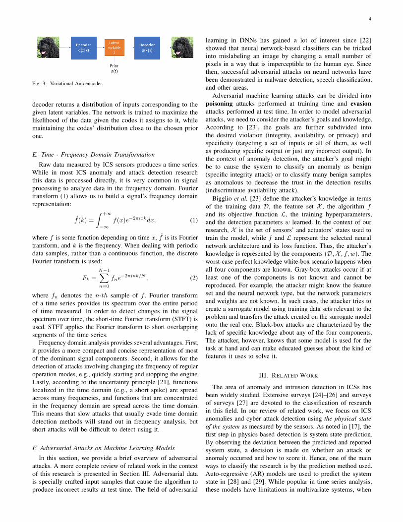
undetected (see Figure 18. However, when we added a singleadditional feature to the model, the adversarial optimizationundid the attacker’s desired physical effect - the adversarialinput conforms to the original model’s prediction and does notcause underflow (see Figures 19 and 20). The same behaviorwas observed with AE-based models. In addition, we observedthat using noise to corrupt the input, as described in SectionII-D increases the robustness of the model to the adversarialevasion abilities even further, because the random noise appliedto the adversarial examples is different between the adversarialtraining and testing time.

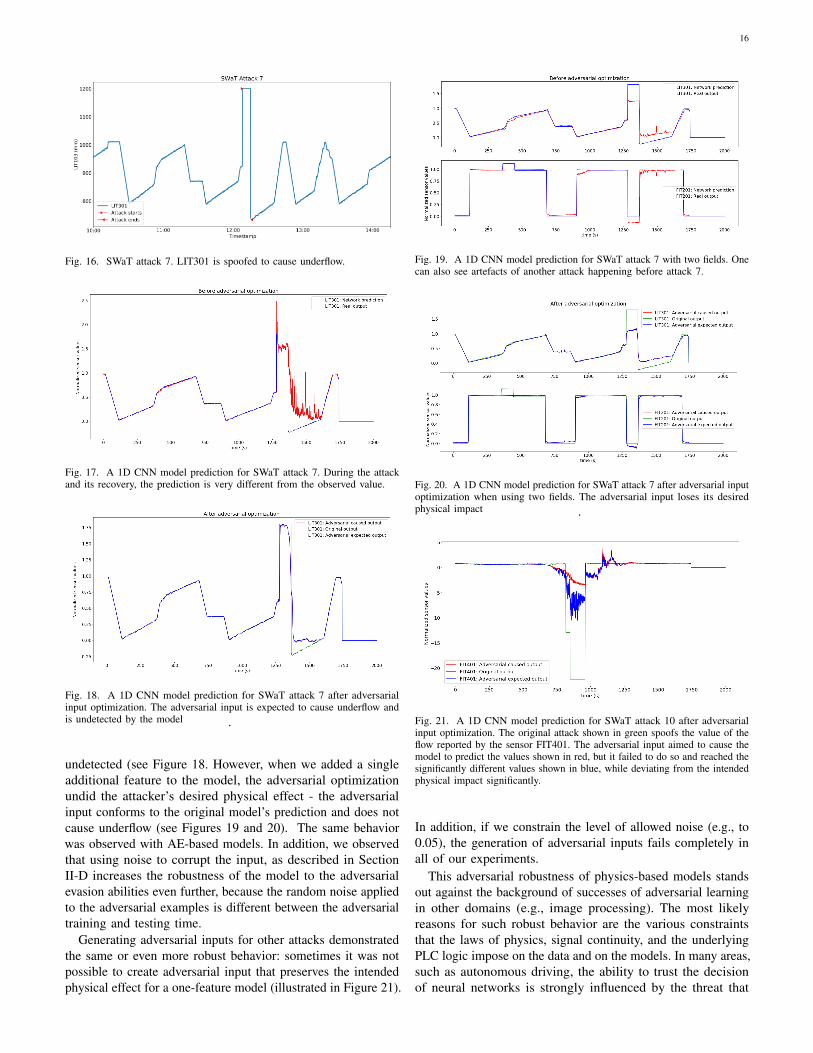
Generating adversarial inputs for other attacks demonstratedthe same or even more robust behavior: sometimes it was notpossible to create adversarial input that preserves the intendedphysical effect for a one-feature model (illustrated in Figure 21).

Fig. 19. A 1D CNN model prediction for SWaT attack 7 with two fields. Onecan also see artefacts of another attack happening before attack 7.

Fig. 20. A 1D CNN model prediction for SWaT attack 7 after adversarial inputoptimization when using two fields. The adversarial input loses its desiredphysical impact .

Fig. 21. A 1D CNN model prediction for SWaT attack 10 after adversarialinput optimization. The original attack shown in green spoofs the value of theflow reported by the sensor FIT401. The adversarial input aimed to cause themodel to predict the values shown in red, but it failed to do so and reached thesignificantly different values shown in blue, while deviating from the intendedphysical impact significantly.

In addition, if we constrain the level of allowed noise (e.g., to0.05), the generation of adversarial inputs fails completely inall of our experiments.

This adversarial robustness of physics-based models standsout against the background of successes of adversarial learningin other domains (e.g., image processing). The most likelyreasons for such robust behavior are the various constraintsthat the laws of physics, signal continuity, and the underlyingPLC logic impose on the data and on the models. In many areas,such as autonomous driving, the ability to trust the decisionof neural networks is strongly influenced by the threat that

17

the decisions were adversarially manipulated. The results ofour experiments suggest that the proposed anomaly detectionmethod is resilient to adversarial evasion attacks that representa major part of adversarial threats.

Despite the promising results, the data-only approach haslimitations:• the tests were conducted only on the attacks present in the

dataset; other attacks for which adversarial input couldbe created might exist,

• the adversarial input generation relies on the model torepresent the real system accurately, however as the attackconditions were never present in the training set, the actualsystem response might be different from the modeled one.

These limitations can be addressed by performing testing on areal system, which is a task for future research.

VII. CONCLUSIONS

In this paper, we studied the effectiveness of 1D CNN andAE-based anomaly and cyber attack detection mechanisms,answering our research questions as follows.• Based on our experiments, we conclude that both 1D

CNNs and AEs achieve or exceed the state-of-the-art per-formance on the three public datasets, while maintaininggenerality, simplicity, and a small footprint. It is not clearwhether one of these architectures is always preferableover another, and we plan to extend our research withmore datasets to investigate this further. In the meantime,we recommend an ensemble consisting of both modelswhen possible. If a single model must be chosen, AEswill likely work out of the box in most cases, while 1DCNNs will require a round of hyperparameter tuning toeliminate false positives.

• We discovered that given the proper data preparationand feature selection, PCA-Reconstruction and windowed-PCA can provide a simple and efficient detector in manypractical cases. Our recommendation is to first try PCAas a baseline detector before applying the neural network-based ones.

• The attack detection method we use allows us to pinpointthe attack location. However, as spoofing attacks cantrigger a number of changes in the related features, all ofthe features will be considered attacked; in such cases, theattack area will be pinpointed still providing significantvalue to the operator. Algorithmic means of distinguishingbetween PLC input and output require the integrationof real-time network data, and this is a topic for futureresearch.

• We found frequency domain analysis helpful in anomalyand attack detection. Its applicability is subject to a numberof practical limitations; if they are met, frequency domainanalysis can provide strong results.

• The proposed detection method was found to be resilientto adversarial evasion attacks. This finding is a promisingone as it allows the operators to trust the decisions of themethod. There is a need to confirm these results with realtestbeds. An additional future research direction is a studyof adversarial poisoning attacks on the proposed method.

VIII. ACKNOWLEDGEMENTS

The authors thank iTrust Centre for Research in CyberSecurity, Singapore University of Technology and Design forcreating and providing the SWaT and WADI datasets, Dr.Elchanan Zwecher for his valuable insights, and Rafael DefenseSystems for supporting this work.

REFERENCES

[1] Wired, “Inside the cunning, unprecedented hack of ukraine’s power grid,”2016, last accessed March 2018. [Online]. Available: https://www.wired.com/2016/03/inside-cunning-unprecedented-hack-ukraines-power-grid/

[2] D. Kushner, “The real story of stuxnet,” ieee Spectrum, vol. 3, no. 50,pp. 48–53, 2013.

[3] ForeignPolicy, “Cyberattack targets safety system at saudi aramco,”2017, last accessed March 2018. [Online]. Available: http://foreignpolicy.com/2017/12/21/cyber-attack-targets-safety-system-at-saudi-aramco/

[4] F. Pasqualetti, F. Dorfler, and F. Bullo, “Cyber-physical attacks in powernetworks: Models, fundamental limitations and monitor design,” inDecision and Control and European Control Conference (CDC-ECC),2011 50th IEEE Conference on. IEEE, 2011, pp. 2195–2201.

[5] A. Teixeira, D. Perez, H. Sandberg, and K. H. Johansson, “Attack modelsand scenarios for networked control systems,” in Proceedings of the 1stinternational conference on High Confidence Networked Systems. ACM,2012, pp. 55–64.

[6] A. Jones, Z. Kong, and C. Belta, “Anomaly detection in cyber-physicalsystems: A formal methods approach,” in Decision and Control (CDC),2014 IEEE 53rd Annual Conference on. IEEE, 2014, pp. 848–853.

[7] V. K. Mishra, V. R. Palleti, and A. Mathur, “A modeling framework forcritical infrastructure and its application in detecting cyber-attacks on awater distribution system,” International Journal of Critical InfrastructureProtection, 2019.

[8] J. M. Beaver, R. C. Borges-Hink, and M. A. Buckner, “An evaluation ofmachine learning methods to detect malicious scada communications,” inMachine Learning and Applications (ICMLA), 2013 12th InternationalConference on, vol. 2. IEEE, 2013, pp. 54–59.

[9] R. C. B. Hink, J. M. Beaver, M. A. Buckner, T. Morris, U. Adhikari,and S. Pan, “Machine learning for power system disturbance and cyber-attack discrimination,” in Resilient Control Systems (ISRCS), 2014 7thInternational Symposium on. IEEE, 2014, pp. 1–8.

[10] J. Goh, S. Adepu, M. Tan, and Z. S. Lee, “Anomaly detection in cyberphysical systems using recurrent neural networks,” in High AssuranceSystems Engineering (HASE), 2017 IEEE 18th International Symposiumon. IEEE, 2017, pp. 140–145.

[11] J. Inoue, Y. Yamagata, Y. Chen, C. M. Poskitt, and J. Sun, “Anomalydetection for a water treatment system using unsupervised machinelearning,” arXiv preprint arXiv:1709.05342, 2017.

[12] Q. Lin, S. Adepu, S. Verwer, and A. Mathur, “Tabor: a graphical model-based approach for anomaly detection in industrial control systems,”in Proceedings of the 2018 on Asia Conference on Computer andCommunications Security. ACM, 2018, pp. 525–536.

[13] M. Kravchik and A. Shabtai, “Detecting cyber attacks in industrial controlsystems using convolutional neural networks,” in Proceedings of the 2018Workshop on Cyber-Physical Systems Security and PrivaCy. ACM,2018, pp. 72–83.

[14] J. Goh, S. Adepu, K. N. Junejo, and A. Mathur, “A dataset to supportresearch in the design of secure water treatment systems,” in InternationalConference on Critical Information Infrastructures Security. Springer,2016, pp. 88–99.

[15] A. Kleinmann, O. Amichay, A. Wool, D. Tenenbaum, O. Bar, and L. Lev,“Stealthy deception attacks against scada systems,” in Computer Security.Springer, 2017, pp. 93–109.

[16] C. M. Ahmed, J. Zhou, and A. P. Mathur, “Noise matters: Usingsensor and process noise fingerprint to detect stealthy cyber attacksand authenticate sensors in cps,” in Proceedings of the 34th AnnualComputer Security Applications Conference. ACM, 2018, pp. 566–581.

[17] J. Giraldo, D. Urbina, A. Cardenas, J. Valente, M. Faisal, J. Ruths, N. O.Tippenhauer, H. Sandberg, and R. Candell, “A survey of physics-basedattack detection in cyber-physical systems,” ACM Computing Surveys(CSUR), vol. 51, no. 4, p. 76, 2018.

[18] Y. LeCun, Y. Bengio et al., “Convolutional networks for images, speech,and time series,” The handbook of brain theory and neural networks,vol. 3361, no. 10, p. 1995, 1995.

18

[19] I. Goodfellow, Y. Bengio, A. Courville, and Y. Bengio, Deep learning.MIT press Cambridge, 2016, vol. 1.

[20] C. Doersch, “Tutorial on variational autoencoders,” arXiv preprintarXiv:1606.05908, 2016.

[21] N. De Bruijn, “Uncertainty principles in fourier analysis,” Inequalities,vol. 2, pp. 57–71, 1967.

[22] C. Szegedy, W. Zaremba, I. Sutskever, J. Bruna, D. Erhan, I. Goodfellow,and R. Fergus, “Intriguing properties of neural networks,” arXiv preprintarXiv:1312.6199, 2013.

[23] B. Biggio and F. Roli, “Wild patterns: Ten years after the rise ofadversarial machine learning,” Pattern Recognition, vol. 84, pp. 317–331,2018.

[24] R. Mitchell and I.-R. Chen, “A survey of intrusion detection techniquesfor cyber-physical systems,” ACM Computing Surveys (CSUR), vol. 46,no. 4, p. 55, 2014.

[25] S. Han, M. Xie, H.-H. Chen, and Y. Ling, “Intrusion detection in cyber-physical systems: Techniques and challenges,” IEEE systems journal,vol. 8, no. 4, pp. 1052–1062, 2014.

[26] A. Humayed, J. Lin, F. Li, and B. Luo, “Cyber-physical systems securityasurvey,” IEEE Internet of Things Journal, vol. 4, no. 6, pp. 1802–1831,2017.

[27] J. Giraldo, E. Sarkar, A. A. Cardenas, M. Maniatakos, and M. Kantar-cioglu, “Security and privacy in cyber-physical systems: A survey ofsurveys,” IEEE Design & Test, vol. 34, no. 4, pp. 7–17, 2017.

[28] D. Hadziosmanovic, R. Sommer, E. Zambon, and P. H. Hartel, “Throughthe eye of the plc: semantic security monitoring for industrial processes,”in Proceedings of the 30th Annual Computer Security ApplicationsConference. ACM, 2014, pp. 126–135.

[29] D. Mashima and A. A. Cardenas, “Evaluating electricity theft detectorsin smart grid networks,” in International Workshop on Recent Advancesin Intrusion Detection. Springer, 2012, pp. 210–229.

[30] S. Mishra, Y. Shoukry, N. Karamchandani, S. N. Diggavi, and P. Tabuada,“Secure state estimation against sensor attacks in the presence of noise,”IEEE Transactions on Control of Network Systems, vol. 4, no. 1, pp.49–59, 2017.

[31] C. Murguia and J. Ruths, “Characterization of a cusum model-basedsensor attack detector,” in 2016 IEEE 55th Conference on Decision andControl (CDC). IEEE, 2016, pp. 1303–1309.

[32] Y. Mo, S. Weerakkody, and B. Sinopoli, “Physical authenticationof control systems: Designing watermarked control inputs to detectcounterfeit sensor outputs,” IEEE Control Systems Magazine, vol. 35,no. 1, pp. 93–109, 2015.

[33] R. Mitchell and R. Chen, “Behavior rule specification-based intrusiondetection for safety critical medical cyber physical systems,” IEEETransactions on Dependable and Secure Computing, vol. 12, no. 1,pp. 16–30, 2015.

[34] M. S. Rahman, M. A. Mahmud, A. M. T. Oo, and H. R. Pota, “Multi-agentapproach for enhancing security of protection schemes in cyber-physicalenergy systems,” IEEE transactions on industrial informatics, vol. 13,no. 2, pp. 436–447, 2016.

[35] T. Roth and B. McMillin, “Physical attestation in the smart grid fordistributed state verification,” IEEE Transactions on Dependable andSecure Computing, vol. 15, no. 2, pp. 275–288, 2018.

[36] W. Aoudi, M. Iturbe, and M. Almgren, “Truth will out: Departure-based process-level detection of stealthy attacks on control systems,” inProceedings of the 2018 ACM SIGSAC Conference on Computer andCommunications Security. ACM, 2018, pp. 817–831.

[37] R. Taormina, S. Galelli, N. O. Tippenhauer, E. Salomons, A. Ostfeld,D. G. Eliades, M. Aghashahi, R. Sundararajan, M. Pourahmadi, M. K.Banks et al., “Battle of the attack detection algorithms: Disclosing cyberattacks on water distribution networks,” Journal of Water ResourcesPlanning and Management, vol. 144, no. 8, p. 04018048, 2018.

[38] M. Housh and Z. Ohar, “Model-based approach for cyber-physical attackdetection in water distribution systems,” Water research, vol. 139, pp.132–143, 2018.

[39] A. Abokifa, K. Haddad, C. Lo, and P. Biswas, “Detection of cyberphysical attacks on water distribution systems via principal componentanalysis and artificial neural networks,” in Proceedings of WorldEnvironmental and Water Resources Congress 2017, 2017, pp. 676–691.

[40] S. Chandy, A. Rasekh, Z. Barker, B. Campbell, and M. Shafiee,“Detection of cyber-attacks to water systems through machine-learning-based anomaly detection in scada data,” in World environmental andwater resources congress, 2017, pp. 611–616.

[41] Y. Mirsky, T. Doitshman, Y. Elovici, and A. Shabtai, “Kitsune: anensemble of autoencoders for online network intrusion detection,” arXivpreprint arXiv:1802.09089, 2018.

[42] M. Sakurada and T. Yairi, “Anomaly detection using autoencoders withnonlinear dimensionality reduction,” in Proceedings of the MLSDA 20142nd Workshop on Machine Learning for Sensory Data Analysis. ACM,2014, p. 4.

[43] R. Taormina and S. Galelli, “Deep-learning approach to the detectionand localization of cyber-physical attacks on water distribution systems,”Journal of Water Resources Planning and Management, vol. 144, no. 10,p. 04018065, 2018.

[44] A. Ghafouri, Y. Vorobeychik, and X. Koutsoukos, “Adversarial regressionfor detecting attacks in cyber-physical systems,” in Proceedings of the27th International Joint Conference on Artificial Intelligence. AAAIPress, 2018, pp. 3769–3775.

[45] C. Feng, T. Li, Z. Zhu, and D. Chana, “A deep learning-based frameworkfor conducting stealthy attacks in industrial control systems,” arXivpreprint arXiv:1709.06397, 2017.

[46] A. Erba, R. Taormina, S. Galelli, M. Pogliani, M. Carminati, S. Zanero,and N. O. Tippenhauer, “Real-time evasion attacks with physicalconstraints on deep learning-based anomaly detectors in industrial controlsystems,” arXiv preprint arXiv:1907.07487, 2019.

[47] R. Taormina, S. Galelli, N. O. Tippenhauer, E. Salomons, and A. Ostfeld,“Characterizing cyber-physical attacks on water distribution systems,”Journal of Water Resources Planning and Management, vol. 143, no. 5,p. 04017009, 2017.

[48] S. E. Chandy, A. Rasekh, Z. A. Barker, and M. E. Shafiee, “Cyberattackdetection using deep generative models with variational inference,”Journal of Water Resources Planning and Management, vol. 145, no. 2,p. 04018093, 2018.

[49] C. M. Ahmed, V. R. Palleti, and A. P. Mathur, “Wadi: A water distributiontestbed for research in the design of secure cyber physical systems,” inProceedings of the 3rd International Workshop on Cyber-Physical Systemsfor Smart Water Networks. ACM, 2017, pp. 25–28.

[50] D. Li, D. Chen, L. Shi, B. Jin, J. Goh, and S.-K. Ng, “Mad-gan:Multivariate anomaly detection for time series data with generativeadversarial networks,” arXiv preprint arXiv:1901.04997, 2019.

[51] I. Chakravati, R. Laha, and J. Roy, “Handbook of methods of appliedstatistics, volume i,” 1967.

[52] M. Natrella et al., “Nist/sematech e-handbook of statistical methods,”Nist/Sematech, vol. 49, 2010.

[53] W. Ku, R. H. Storer, and C. Georgakis, “Disturbance detection andisolation by dynamic principal component analysis,” Chemometrics andintelligent laboratory systems, vol. 30, no. 1, pp. 179–196, 1995.

[54] D. E. Goldberg and J. H. Holland, “Genetic algorithms and machinelearning,” Machine learning, vol. 3, no. 2, pp. 95–99, 1988.

Moshe Kravchik received his M.Sc. (2007) incomputer science from the Open University of Israel.He is currently pursuing a Ph.D. at Ben-GurionUniversity of the Negev and teaches cyber securityat Lev Academic Centre in Jerusalem. His researchinterests include the topics of software and systemssecurity, trusted execution environments, anomalydetection, and the security of industrial controlsystems.

Asaf Shabtai Asaf Shabtai is a professor in theDepartment of Software and Information SystemsEngineering at Ben-Gurion University of the Negev.His main areas of interest are computer and networksecurity, machine learning, security of IoT and smartmobile devices, social network analysis, and securityof avionic and operational technology (OT) systems.Asaf holds a B.Sc. in mathematics and computerSciences; B.Sc. in information systems engineering;M.Sc. in information systems engineering and a Ph.D.in information systems engineering all from Ben-

Gurion University.