EEL5840: Machine Intelligence Introduction to feedforward ... · train artiﬁcial neural networks to model input/output data; that is, how learning occurs in artiﬁcial neural net-works

EEL5840: Machine Intelligence Introduction to feedforward neural networks

Introduction to feedforward neural networks

1. Problem statement and historical context

A. Learning framework

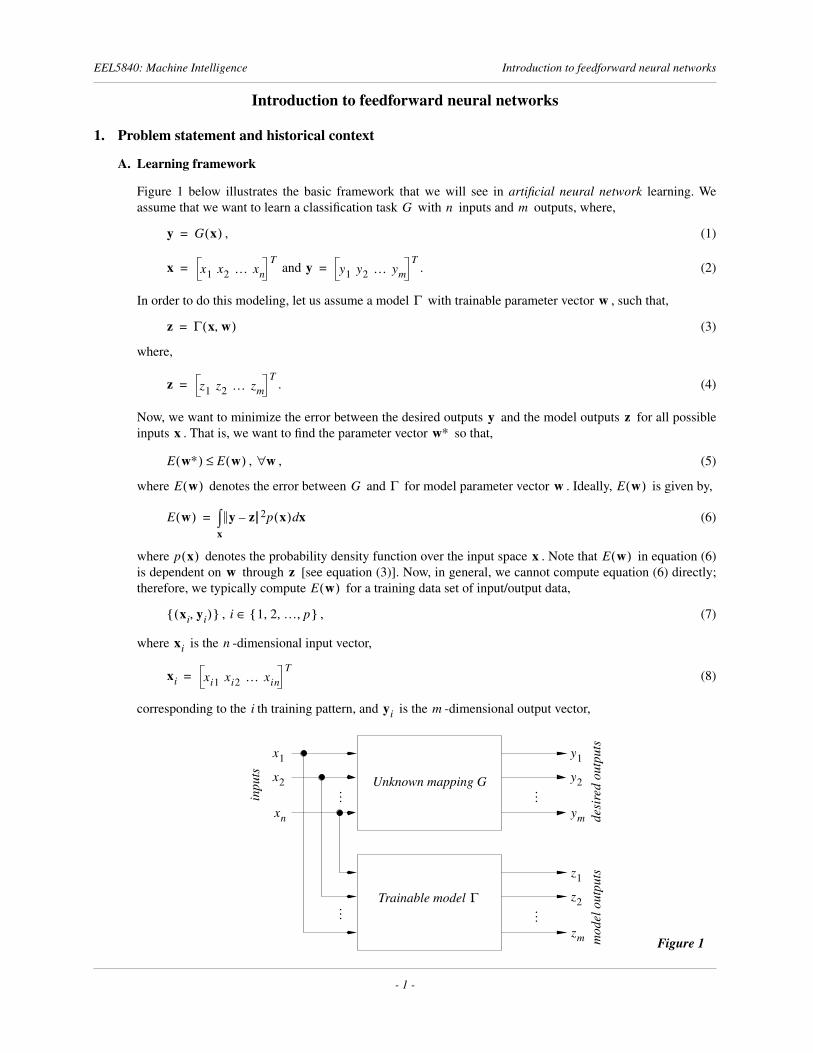
Figure 1 below illustrates the basic framework that we will see in artificial neural network learning. Weassume that we want to learn a classification task with inputs and outputs, where,

, (1)

and . (2)

In order to do this modeling, let us assume a model with trainable parameter vector , such that,

(3)

where,

. (4)

Now, we want to minimize the error between the desired outputs and the model outputs for all possibleinputs . That is, we want to find the parameter vector so that,

, , (5)

where denotes the error between and for model parameter vector . Ideally, is given by,

(6)

where denotes the probability density function over the input space . Note that in equation (6)is dependent on through [see equation (3)]. Now, in general, we cannot compute equation (6) directly;therefore, we typically compute for a training data set of input/output data,

, , (7)

where is the -dimensional input vector,

(8)

corresponding to the th training pattern, and is the -dimensional output vector,

G n m

x1

Figure 1

x2

xn

… …

y1

y2

ym

…

z1

z2

zm

…

Unknown mapping G

Trainable model Γ

inpu

ts

mod

el o

utpu

tsde

sire

d ou

tput

s

y G x( )=

x x1 x2 … xnT

= y y1 y2 … ymT

=

Γ w

z Γ x w,( )=

z z1 z2 … zmT

=

y zx w∗

E w∗( ) E w( )≤ w∀

E w( ) G Γ w E w( )

E w( ) y z– 2p x( ) xdx∫=

p x( ) x E w( )w z

E w( )

xi yi,( ){ } i 1 2 … p, , ,{ }∈

xi n

xi xi1 xi2 … xinT

=

i yi m

- 1 -


(9)

corresponding to the th training pattern, . For (7), we can define the computable error func-tion ,

(10)

where,

. (11)

If the data set is well distributed over possible inputs, equation (10) gives a good approximation of the errormeasure in (6).

As we shall see shortly, artificial neural networks are one type of parametric model for which we can min-imize the error measure in equation (10) over a given training data set. Simply put, artificial neural networksare nonlinear function approximators, with adjustable (i.e. trainable) parameters , that allow us to modelfunctional mappings, including classification tasks, between inputs and outputs.

B. Biological inspiration

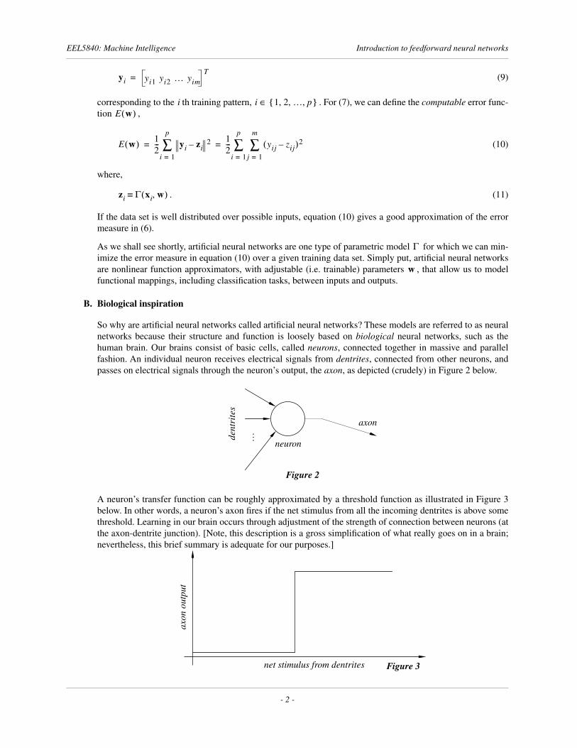
So why are artificial neural networks called artificial neural networks? These models are referred to as neuralnetworks because their structure and function is loosely based on biological neural networks, such as thehuman brain. Our brains consist of basic cells, called neurons, connected together in massive and parallelfashion. An individual neuron receives electrical signals from dentrites, connected from other neurons, andpasses on electrical signals through the neuron’s output, the axon, as depicted (crudely) in Figure 2 below.

A neuron’s transfer function can be roughly approximated by a threshold function as illustrated in Figure 3below. In other words, a neuron’s axon fires if the net stimulus from all the incoming dentrites is above somethreshold. Learning in our brain occurs through adjustment of the strength of connection between neurons (atthe axon-dentrite junction). [Note, this description is a gross simplification of what really goes on in a brain;nevertheless, this brief summary is adequate for our purposes.]

yi yi1 yi2 … yimT

=

i i 1 2 … p, , ,{ }∈E w( )

E w( ) 12--- yi zi– 2

i 1=

p

∑ 12--- yij zij–( )2

j 1=

m

∑i 1=

p

∑= =

zi Γ xi w,( )≡

Γ

w

Figure 2

…

dent

rite

s

axon

neuron

Figure 3net stimulus from dentrites

axon

out

put

- 2 -


Now, artificial neural networks attempt to crudely emulate biological neural networks in the following impor-tant ways:

1. Simple basic units are the building blocks of artificial neural networks. It is important to note that artificial “neurons” are much, much simpler than their biological counterparts.

2. Individual units are connected massively and in parallel.

3. Individual units have threshold-type activation functions.

4. Learning in artificial neural networks occurs by adjusting the strength of connection between individual units. These parameters are known as the weights of the neural network.

We point out that artificial neural networks are much, much, much simpler than complex biological neuralnetworks (like the human brain). According to the Encyclopedia Britannica, the average human brain consistsof approximately individual neurons with approximately connections. Even very complicatedartificial neural networks typically do not have more than to connections between, at most, individual basic units.

As of September, 2001, an INSPEC database search generated over 45,000 hits with the keyword “neural net-work.” Considering that neural network research did not really take off until 1986, with the publication of thebackpropagation training algorithm, we see that research in artificial neural networks has exploded over thepast 15 years and is still quite active today. We will try to cover some of the highlights of that research. First,however, we will formalize our discussion above, clearly defining what a neural network is, and how we cantrain artificial neural networks to model input/output data; that is, how learning occurs in artificial neural net-works.

2. What makes a neural network a neural network?

A. Basic building blocks of neural networks

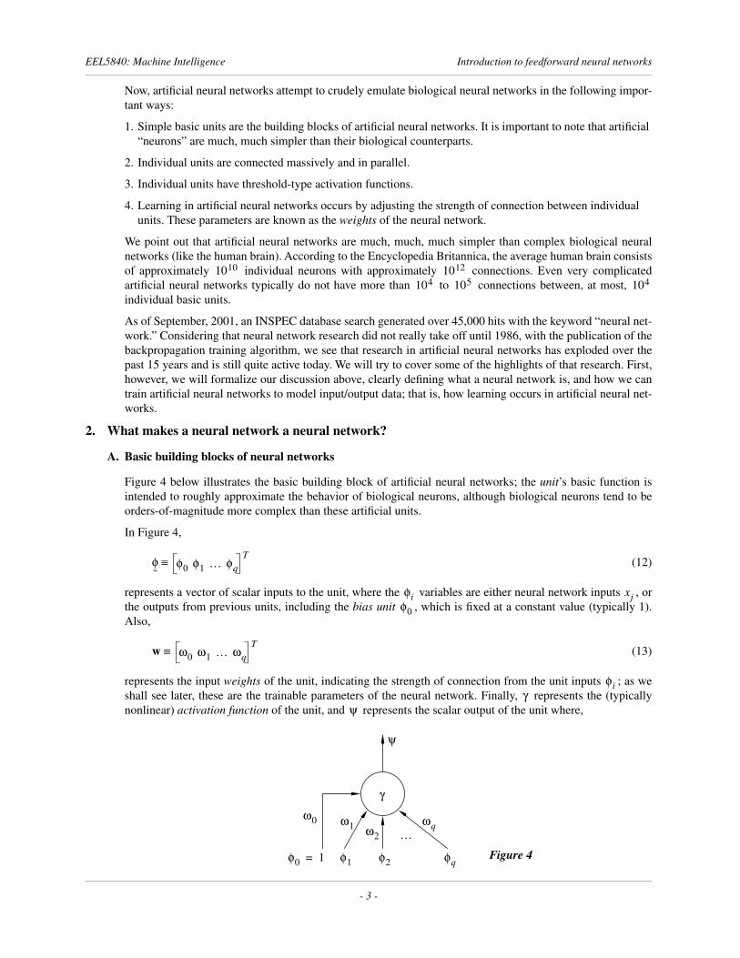
Figure 4 below illustrates the basic building block of artificial neural networks; the unit’s basic function isintended to roughly approximate the behavior of biological neurons, although biological neurons tend to beorders-of-magnitude more complex than these artificial units.

In Figure 4,

(12)

represents a vector of scalar inputs to the unit, where the variables are either neural network inputs , orthe outputs from previous units, including the bias unit , which is fixed at a constant value (typically 1).Also,

(13)

represents the input weights of the unit, indicating the strength of connection from the unit inputs ; as weshall see later, these are the trainable parameters of the neural network. Finally, represents the (typicallynonlinear) activation function of the unit, and represents the scalar output of the unit where,

1010 1012

104 105 104

Figure 4

ω0

ψ

γ

…ω1 ω2

ωq

φ0 1= φ1 φ2 φq

φ˜

φ0 φ1 … φqT

≡

φi xjφ0

w ω0 ω1 … ωqT

≡

φiγ

ψ

- 3 -


(14)

Thus, a unit in an artificial neural network sums up its total input and passes that sum through some (in gen-eral) nonlinear activation function.

B. Perceptrons

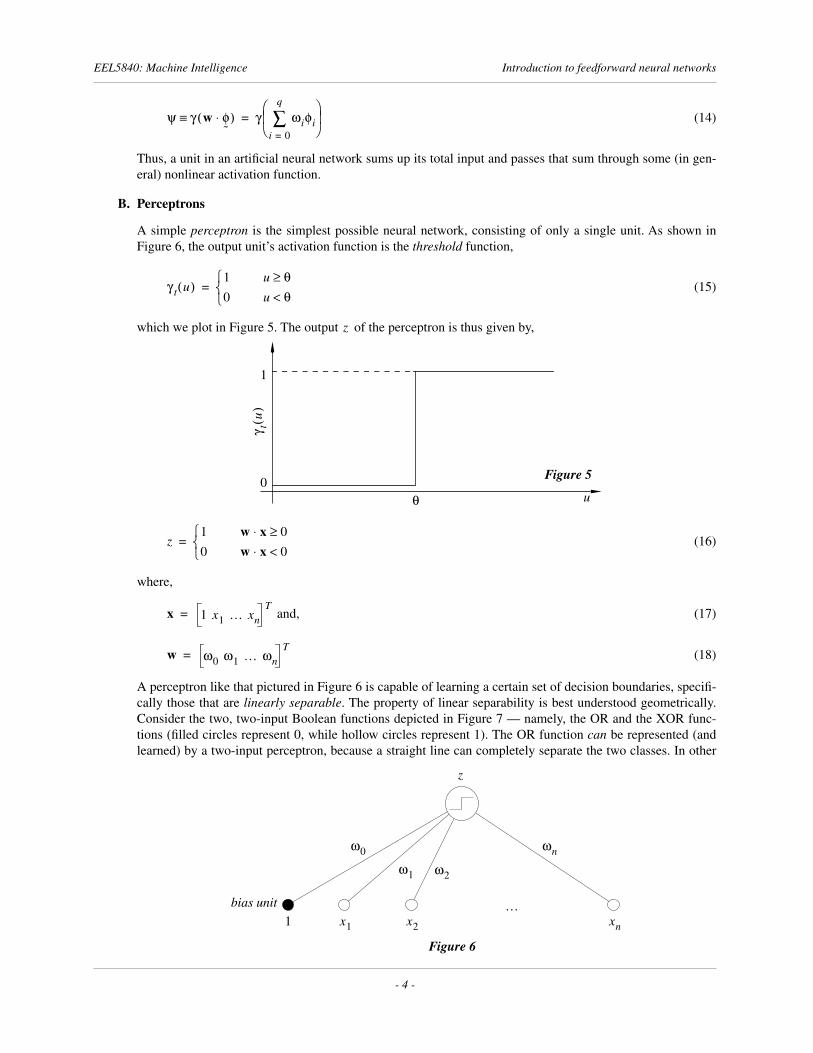
A simple perceptron is the simplest possible neural network, consisting of only a single unit. As shown inFigure 6, the output unit’s activation function is the threshold function,

(15)

which we plot in Figure 5. The output of the perceptron is thus given by,

(16)

where,

and, (17)

(18)

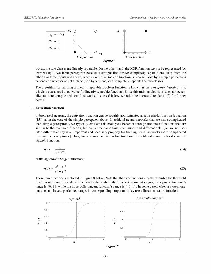
A perceptron like that pictured in Figure 6 is capable of learning a certain set of decision boundaries, specifi-cally those that are linearly separable. The property of linear separability is best understood geometrically.Consider the two, two-input Boolean functions depicted in Figure 7 — namely, the OR and the XOR func-tions (filled circles represent 0, while hollow circles represent 1). The OR function can be represented (andlearned) by a two-input perceptron, because a straight line can completely separate the two classes. In other

ψ γ w φ˜

⋅( )≡ γ ωiφii 0=

q

∑

=

γ t u( )1 u θ≥0 u θ<

=

γ tu(

)

u

Figure 50

1

θ

z

z1 w x⋅ 0≥0 w x⋅ 0<

=

x 1 x1 … xnT

=

w ω0 ω1 … ωnT

=

x1 x2 xn

z

…bias unit1

Figure 6

ωn

ω2ω1

ω0

- 4 -


words, the two classes are linearly separable. On the other hand, the XOR function cannot be represented (orlearned) by a two-input perceptron because a straight line cannot completely separate one class from theother. For three inputs and above, whether or not a Boolean function is representable by a simple perceptrondepends on whether or not a plane (or a hyperplane) can completely separate the two classes.

The algorithm for learning a linearly separable Boolean function is known as the perceptron learning rule,which is guaranteed to converge for linearly separable functions. Since this training algorithm does not gener-alize to more complicated neural networks, discussed below, we refer the interested reader to [2] for furtherdetails.

C. Activation function

In biological neurons, the activation function can be roughly approximated as a threshold function [equation(15)], as in the case of the simple perceptron above. In artificial neural networks that are more complicatedthan simple perceptrons, we typically emulate this biological behavior through nonlinear functions that aresimilar to the threshold function, but are, at the same time, continuous and differentiable. [As we will seelater, differentiability is an important and necessary property for training neural networks more complicatedthan simple perceptrons.] Thus, two common activation functions used in artificial neural networks are thesigmoid function,

(19)

or the hyperbolic tangent function,

(20)

These two functions are plotted in Figure 8 below. Note that the two functions closely resemble the thresholdfunction in Figure 5 and differ from each other only in their respective output ranges; the sigmoid function’srange is , while the hyperbolic tangent function’s range is . In some cases, when a system out-put does not have a predefined range, its corresponding output unit may use a linear activation function,

0.2 0.4 0.6 0.8 1

0.2

0.4

0.6

0.8

1

0.2 0.4 0.6 0.8 1

0.2

0.4

0.6

0.8

1

OR function XOR functionFigure 7

x2

x1

x2

x1

ω0 0.5–=

ω1 1=

ω2 1=

γ u( ) 11 e u–+-----------------=

γ u( ) eu e u––eu e u–+-------------------=

0 1,[ ] 1– 1,[ ]

-10 -5 0 5 100

0.2

0.4

0.6

0.8

1

γu(

)

u-10 -5 0 5 10

-1

-0.5

0

0.5

1

Figure 8

γu(

)

u

sigmoid hyperbolic tangent

- 5 -


(21)

From Figure 8, the role of the bias unit should now be a little clearer; its role is essentially equivalent tothe threshold parameter in Figure 5, allowing the unit output to be shifted along the horizontal axis.

D. Neural network architectures

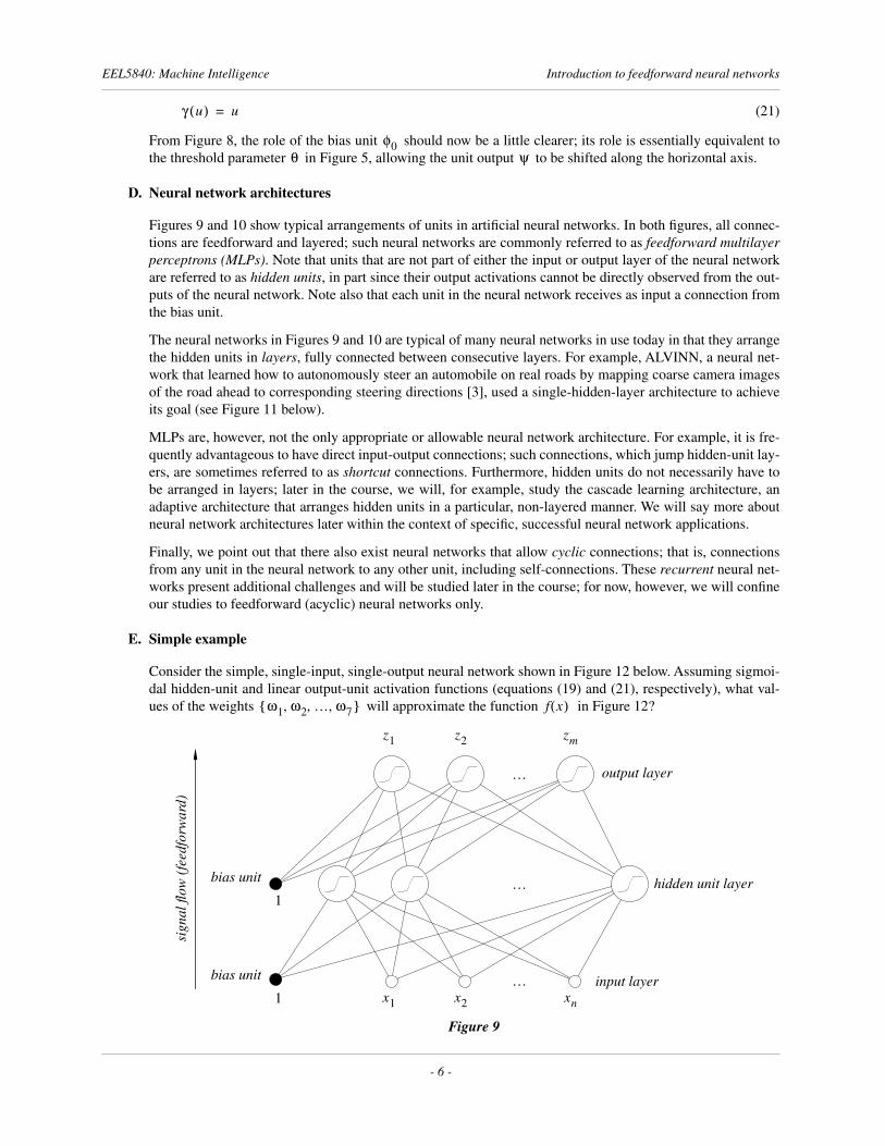
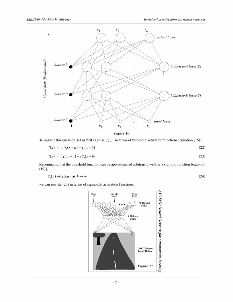
Figures 9 and 10 show typical arrangements of units in artificial neural networks. In both figures, all connec-tions are feedforward and layered; such neural networks are commonly referred to as feedforward multilayerperceptrons (MLPs). Note that units that are not part of either the input or output layer of the neural networkare referred to as hidden units, in part since their output activations cannot be directly observed from the out-puts of the neural network. Note also that each unit in the neural network receives as input a connection fromthe bias unit.

The neural networks in Figures 9 and 10 are typical of many neural networks in use today in that they arrangethe hidden units in layers, fully connected between consecutive layers. For example, ALVINN, a neural net-work that learned how to autonomously steer an automobile on real roads by mapping coarse camera imagesof the road ahead to corresponding steering directions [3], used a single-hidden-layer architecture to achieveits goal (see Figure 11 below).

MLPs are, however, not the only appropriate or allowable neural network architecture. For example, it is fre-quently advantageous to have direct input-output connections; such connections, which jump hidden-unit lay-ers, are sometimes referred to as shortcut connections. Furthermore, hidden units do not necessarily have tobe arranged in layers; later in the course, we will, for example, study the cascade learning architecture, anadaptive architecture that arranges hidden units in a particular, non-layered manner. We will say more aboutneural network architectures later within the context of specific, successful neural network applications.

Finally, we point out that there also exist neural networks that allow cyclic connections; that is, connectionsfrom any unit in the neural network to any other unit, including self-connections. These recurrent neural net-works present additional challenges and will be studied later in the course; for now, however, we will confineour studies to feedforward (acyclic) neural networks only.

E. Simple example

Consider the simple, single-input, single-output neural network shown in Figure 12 below. Assuming sigmoi-dal hidden-unit and linear output-unit activation functions (equations (19) and (21), respectively), what val-ues of the weights will approximate the function in Figure 12?

γ u( ) u=

φ0θ ψ

Figure 9

x1 x2 xn

z1 z2 zm

…

…

…

1

1

output layer

hidden unit layer

input layer

bias unit

bias unit

sign

al fl

ow (f

eedf

orw

ard)

ω1 ω2 … ω7, , ,{ } f x( )

- 6 -


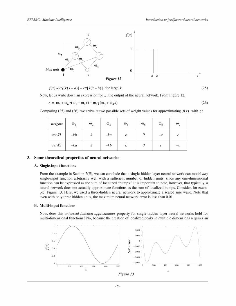
To answer this question, let us first express in terms of threshold activation functions [equation (15)]:

(22)

(23)

Recognizing that the threshold function can be approximated arbitrarily well by a sigmoid function [equation(19)],

as (24)

we can rewrite (23) in terms of sigmoidal activation functions,

Figure 10

output layer

hidden unit layer #2

input layer

bias unit

bias unit

sign

al fl

ow (f

eedf

orw

ard)

x1 x2 xn

z1 z2 zm

…

…

……

…

bias unit

1

1

1

hidden unit layer #1

Sharp Left

SharpRight

4 Hidden Units

30 Output Units

30x32 Sensor Input Retina

Straight Ahead

ALV

INN

: Neural N

etwork for Autonom

ous Steering

Figure 11

f x( )

f x( ) c γ t x a–( ) γ t x b–( )–[ ]=

f x( ) cγ t x a–( ) cγ t x b–( )–=

γ t u( ) γ ku( )→ k ∞→

- 7 -


for large . (25)

Now, let us write down an expression for , the output of the neural network. From Figure 12,

(26)

Comparing (25) and (26), we arrive at two possible sets of weight values for approximating with :

3. Some theoretical properties of neural networks

A. Single-input functions

From the example in Section 2(E), we can conclude that a single-hidden layer neural network can model anysingle-input function arbitrarily well with a sufficient number of hidden units, since any one-dimensionalfunction can be expressed as the sum of localized “bumps.” It is important to note, however, that typically, aneural network does not actually approximate functions as the sum of localized bumps. Consider, for exam-ple, Figure 13. Here, we used a three-hidden neural network to approximate a scaled sine wave. Note thateven with only three hidden units, the maximum neural network error is less than 0.01.

B. Multi-input functions

Now, does this universal function approximator property for single-hidden layer neural networks hold formulti-dimensional functions? No, because the creation of localized peaks in multiple dimensions requires an

weights

set #1 0

set #2 0

a b

c

0x

f x( )

Figure 12

bias unit

z

x1

ω1ω2

ω4ω3

ω6

ω5

ω7

f x( ) cγ k x a–( )[ ] cγ k x b–( )[ ]–≈ k

z

z ω5 ω6γ ω1 ω2x+( ) ω7γ ω3 ω4x+( )+ +=

f x( ) z

ω1 ω2 ω3 ω4 ω5 ω6 ω7

kb– k ka– k c– c

ka– k kb– k c c–

Figure 13

0 200 400 600 800 10000

0.2

0.4

0.6

0.8

1

0 200 400 600 800 1000-0.008

-0.006

-0.004

-0.002

0

0.002

0.004

fx(

)

x x

NN

err

or

- 8 -


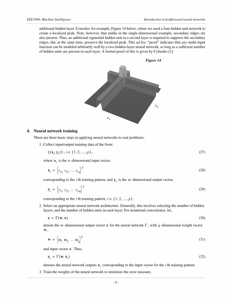
additional hidden layer. Consider, for example, Figure 14 below, where we used a four-hidden unit network tocreate a localized peak. Note, however, that unlike in the single-dimensional example, secondary ridges arealso present. Thus, an additional sigmoidal hidden unit in a second layer is required to suppress the secondaryridges, but, at the same time, preserve the localized peak. This ad hoc “proof” indicates that any multi-inputfunction can be modeled arbitrarily well by a two-hidden-layer neural network, as long as a sufficient numberof hidden units are present in each layer. A formal proof of this is given by Cybenko [1].

4. Neural network trainingThere are three basic steps in applying neural networks to real problems:

1. Collect input/output training data of the form:

, , (27)

where is the -dimensional input vector,

(28)

corresponding to the th training pattern, and is the -dimensional output vector,

(29)

corresponding to the th training pattern, .

2. Select an appropriate neural network architecture. Generally, this involves selecting the number of hidden layers, and the number of hidden units in each layer. For notational convenience, let,

(30)

denote the -dimensional output vector for the neural network , with -dimensional weight vector ,

(31)

and input vector . Thus,

(32)

denotes the neural network outputs corresponding to the input vector for the th training pattern.

3. Train the weights of the neural network to minimize the error measure,

x1

x2

Figure 14

xi yi,( ){ } i 1 2 … p, , ,{ }∈

xi n

xi xi1 xi2 … xinT

=

i yi m

yi yi1 yi2 … yimT

=

i i 1 2 … p, , ,{ }∈

z Γ w x,( )=

m z Γ qw

w ω1 ω2 … ωqT

=

x

zi Γ w xi,( )=

zi i

- 9 -


(33)

which measures the difference between the neural network outputs and the training data outputs . This error minimization is also frequently referred to as learning.

Steps 1 and 2 above are quite application specific and will be discussed a little later. Here, we will begin to inves-tigate Step 3 — namely, the training of the neural network parameters (weights) from input/output training data.

A. Gradient descent

Note that since (as defined in equation (32) above) is a function of the weights of the neural network, is implicitly a function of those weights as well. That is, changes as a function of . Therefore, our goal isto find that set of weights which minimizes over a given training data set.

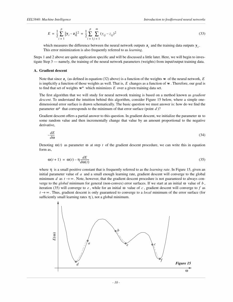
The first algorithm that we will study for neural network training is based on a method known as gradientdescent. To understand the intuition behind this algorithm, consider Figure 15 below, where a simple one-dimensional error surface is drawn schematically. The basic question we must answer is: how do we find theparameter that corresponds to the minimum of that error surface (point )?

Gradient descent offers a partial answer to this question. In gradient descent, we initialize the parameter tosome random value and then incrementally change that value by an amount proportional to the negativederivative,

(34)

Denoting as parameter at step of the gradient descent procedure, we can write this in equationform as,

(35)

where is a small positive constant that is frequently referred to as the learning rate. In Figure 15, given aninitial parameter value of and a small enough learning rate, gradient descent will converge to the globalminimum as . Note, however, that the gradient descent procedure is not guaranteed to always con-verge to the global minimum for general (non-convex) error surfaces. If we start at an initial value of ,iteration (35) will converge to , while for an initial value of , gradient descent will converge to as

. Thus, gradient descent is only guaranteed to converge to a local minimum of the error surface (forsufficiently small learning rates ), not a global minimum.

E 12--- yi zi– 2

i 1=

p

∑ 12--- yij zij–( )2

j 1=

m

∑i 1=

p

∑= =

zi yi

zi w EE w

w∗ E

ω∗ d

b

c

d

e

f

Eω(

)

a

ω

Figure 15

ω

dEdω-------–

ω t( ) ω t

ω t 1+( ) ω t( ) η dEdω t( )--------------–=

ηa

d t ∞→ω b

e ω c ft ∞→

η

- 10 -


Iteration (35) is easily generalized to error minimization over multiple dimensions (i.e. parameter vectors ),

(36)

where denotes the gradient of with respect to ,

(37)

Thus, one approach for training the weights in a neural network implements iteration (37) with the error mea-sure defined in equation (33).

B. Simple example

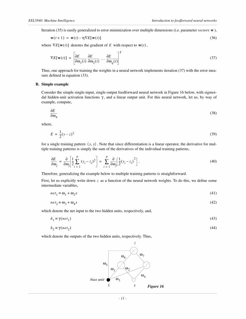
Consider the simple single-input, single-output feedforward neural network in Figure 16 below, with sigmoi-dal hidden-unit activation functions , and a linear output unit. For this neural network, let us, by way ofexample, compute,

(38)

where,

(39)

for a single training pattern . Note that since differentiation is a linear operator, the derivative for mul-tiple training patterns is simply the sum of the derivatives of the individual training patterns,

. (40)

Therefore, generalizing the example below to multiple training patterns is straightforward.

First, let us explicitly write down as a function of the neural network weights. To do this, we define someintermediate variables,

(41)

(42)

which denote the net input to the two hidden units, respectively, and,

(43)

(44)

which denote the outputs of the two hidden units, respectively. Thus,

w

w t 1+( ) w t( ) η E w t( )[ ]∇–=

E w t( )[ ]∇ E w t( )

E w t( )[ ]∇ω1 t( )∂

∂Eω2 t( )∂

∂E … ωq t( )∂∂E

T

=

γ

Figure 16

bias unit

z

x1

ω1ω2

ω4ω3

ω6

ω5

ω7

ω4∂∂E

E 12--- y z–( )2=

x y,⟨ ⟩

ωj∂∂E

ωj∂∂ 1

2--- yi zi–( )2

i 1=

p

∑ ωj∂∂ 1

2--- yi zi–( )

2

i 1=

p

∑= =

z

net1 ω1 ω2x+≡

net2 ω3 ω4x+≡

h1 γ net1( )≡

h2 γ net2( )≡

- 11 -


(linear output unit). (45)

Now, we can compute the derivative of with respect to . From (39), and remembering the chain rule ofdifferentiation,

(46)

(47)

(48)

where denotes the derivative of the activation function. This example shows that, in principle, computingthe partial derivatives required for the gradient descent algorithm simply requires careful application of thechain rule. In general, however, we would like to be able to simulate neural networks whose architecture isnot known a priori. In other words, rather than hard-code derivatives with explicit expressions like (48)above, we require an algorithm which allows us to compute derivatives in a more general way. Such an algo-rithm exists, and is known as the backpropagation algorithm.

C. Backpropagation algorithm

The backpropagation algorithm was first published by Rumelhart and McClelland in 1986 [4], and has sinceled to an explosion in previously dormant neural-network research. Backpropagation offers an efficient, algo-rithmic formulation for computing error derivatives with respect to the weights of a neural network. As such,it allows us to implement gradient descent for neural network training without explicitly hard-coding deriva-tives.

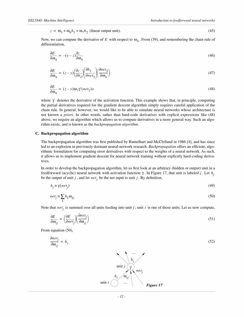
In order to develop the backpropagation algorithm, let us first look at an arbitrary (hidden or output) unit in afeedforward (acyclic) neural network with activation function . In Figure 17, that unit is labeled . Let be the output of unit , and let be the net input to unit . By definition,

(49)

(50)

Note that is summed over all units feeding into unit ; unit is one of those units. Let us now compute,

(51)

From equation (50),

(52)

z ω5 ω6h1 ω7h2+ +=

E ω4

ω4∂∂E y z–( ) ω4∂

∂z–=

ω4∂∂E z y–( )

h2∂∂z

net2∂∂h2

net2∂

∂ω4-------------

=

ω4∂∂E z y–( )ω7γ'net2( )x=

γ'

γ j hjj netj j

hj γ netj( )≡

netj hkωkjk∑≡

…

Figure 17

hj

ωij

γ

hi

…

netj

unit j

unit i

netj j i

ωij∂∂E

netj∂∂E

netj∂

ωij∂------------

=

netj∂ωij∂

------------ hi=

- 12 -


since all the terms in summation (50), are independent of . Defining,

(53)

we can write equation (51) as,

(54)

As we will see shortly, equation (54) forms the basis of the backpropagation algorithm in that the variablescan be computed recursively from the outputs of the neural network back to the inputs of the neural network.In other words, the values are backpropagated through the network (hence, the name of the algorithm).

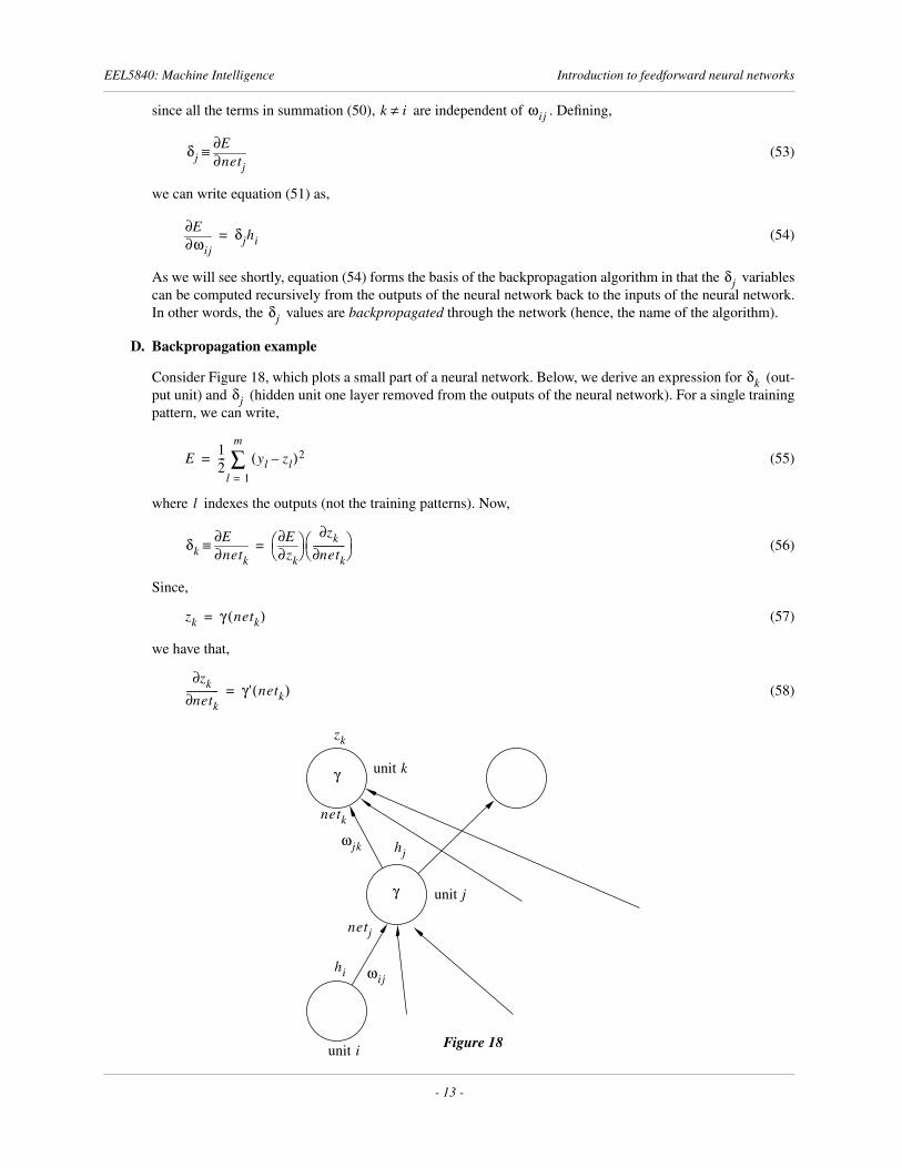
D. Backpropagation example

Consider Figure 18, which plots a small part of a neural network. Below, we derive an expression for (out-put unit) and (hidden unit one layer removed from the outputs of the neural network). For a single trainingpattern, we can write,

(55)

where indexes the outputs (not the training patterns). Now,

(56)

Since,

(57)

we have that,

(58)

k i≠ ωij

δj netj∂∂E≡

ωij∂∂E δjhi=

δj

δj

δkδj

zk

Figure 18

hjωjk

netk

netj

γ

ωijhi

γ unit j

unit i

unit k

E 12--- yl zl–( )2

l 1=

m

∑=

l

δk netk∂∂E≡

zk∂∂E

zk∂

netk∂-------------

=

zk γ netk( )=

zk∂netk∂

------------- γ'netk( )=

- 13 -


Furthermore, from equation (55),

(59)

since all the terms in summation (55), are independent of . Combining equations (56), (58) and (59),and recalling equation (54),

(60)

(61)

Note that equations (60) and (61) are valid for any weight in a neural network that is connected to an outputunit. Also note that is the output value of units feeding into output unit . While this may be the output ofa hidden unit, it could also be the output of the bias unit (i.e. 1) or the value of a neural network input (i.e. ).Next, we want to compute in Figure 18 in terms of the values that follow unit . Going back to defini-tion (53),

(62)

Note that the summation in equation (62) is over all the immediate successor units of unit . Thus,

(63)

By definition,

(64)

So, from equation (64),

(65)

since all the terms in summation (64), are independent of . Combining equations (63) and (65),

(66)

(67)

(68)

Note that equation (67) computes in terms of those values one connection ahead of unit . In otherwords, the values are backpropagated from the outputs back through the network. Also note that is theoutput value of units feeding into unit . While this may be the output of a hidden unit from an earlier hidden-unit layer, it could also be the output of a bias unit (i.e. 1) or the value of a neural network input (i.e. ).

It is important to note that (1) the general derivative expression in (54) is valid for all weights in the neuralnetwork; (2) the expression for the output values in (60) is valid for all neural network output units; and (3)the recursive relationship for in (67) is valid for all hidden units, where the -indexed summation is overall immediate successors of unit .

zk∂∂E zk yk–( )=

l k≠ zk

δk zk yk–( )γ'netk( )=

ωjk∂∂E δkhj=

hj kxj

δj δ j

δj netj∂∂E≡

netl∂∂E

netl∂

netj∂------------

l

∑=

j

δj δl

netl∂netj∂

------------

l∑=

netl ωslγ nets( )s∑=

netl∂netj∂

------------ ωjlγ'netj( )=

s j≠ netj

δj δlωjlγ'netj( )l

∑=

δj δlωjll

∑ γ'netj( )=

ωij∂∂E δjhi=

δj δ jδ hi

jxi

δδj l

j

- 14 -


E. Summary of backpropagation algorithm

Below, we summarize the results of the derivation in the previous section. The partial derivative of the error,

(69)

(i.e. a single training pattern) with respect to a weight connected to output unit of a neural network isgiven by,

(70)

(71)

where is the output of hidden unit (or the input ), and is the net input to output unit . The partialderivative of the error with respect to a weight connected to hidden unit of a neural network is givenby,

(72)

(73)

where is the output of hidden unit (or the input ), and is the net input to hidden unit . The aboveresults are trivially extended to multiple training patterns by summing the results for individual training pat-terns over all training patterns.

5. Basic steps in using neural networksSo, now we know what a neural network is, and we know a basic algorithm for training neural networks (i.e.backpropagation). Here, we will extend our discussion of neural networks by discussing some practical aspectsof applying neural networks to real-world problems. Below, we review the steps that need to be followed in usingneural networks.

A. Collect training data

In order to apply a neural network to a problem, we must first collect input/output training data that ade-quately represents that problem. Often, we also need to condition, or preprocess that data so that the neuralnetwork training converges more quickly and/or to better local minima of the error surface. Data collectionand preprocessing is very application-dependent and will be discussed in greater detail in the context of spe-cific applications.

B. Select neural network architecture

Selecting a neural network architecture typically requires that we determine (1) an appropriate number ofhidden layers and (2) an appropriate number of hidden units in each hidden layer for our specific application,assuming a standard multilayer feedforward architecture. Often, there will be many different neural networkstructures that work about equally well; which structures are most appropriate is frequently guided by experi-ence and/or trial-and-error. Alternatively, as we will talk about later in this course, we can use neural networklearning algorithms that adaptively change the structure of the neural network as part of the learning process.

C. Select learning algorithm

If we use simple backpropagation, we must select an appropriate learning rate . Alternatively, as we willtalk about later in this course, we have a choice of more sophisticated learning algorithms as well, includingthe conjugate gradient and extended Kalman filtering methods.

E 12--- yl zl–( )2

l 1=

m

∑=

ωjk k

δk zk yk–( )γ'netk( )=

ωjk∂∂E δkhj=

hj j j netk kE ωij j

δj δlωjll

∑ γ'netj( )=

ωij∂∂E δjhi=

hi i i netj j

η

- 15 -


D. Weight initialization

Weights in the neural network are usually initialized to small, random values.

E. Forward pass

Apply a random input vector from the training data set to the neural network and compute the neural net-work outputs , the hidden-unit outputs , and the net input to each hidden unit .

F. Backward pass

1. Evaluate at the outputs, where,

(74)

for each output unit.

2. Backpropagate the values from the outputs backwards through the neural network.

3. Using the computed values, calculate,

, (75)

the derivative of the error with respect to each weight in the neural network.

4. Update the weights based on the computed gradient,

. (76)

G. Loop

Repeat steps E and F (forward and backward passes) until training results in a satisfactory model.

6. Practical issues in neural networks

A. What should the training data be?

Some questions that need to be answered include:

1. Is your training data sufficient for the neural network to adequately learn what you want it to learn? For example, what if, in ALVINN [3], we down-sampled to images, instead of images? Such coarse images would probably not suffice for learning the steering of the on-road vehicle with enough accuracy. At the same time we must make sure that we don’t include training data that is too much or irrel-evant for our application (e.g. for ALVINN, music played while driving). Poorly correlated or irrelevant inputs can easily slowdown convergence of, or completely sidetrack, neural network learning algorithms.

2. Is your training data biased? Suppose for ALVINN, we trained the neural network on race track oval. How would ALVINN drive on real roads? Well, it would probably not have adequately learned right turns, since the race track consists of left turns only. The distribution of your training data needs to approximately reflect the expected distribution of input data where the neural network will be used after training.

3. Is your task deterministic or stochastic? Is it stationary or nonstationary? Nonstationary problems cannot be trained from fixed data sets, since, by definition, things change over time.

We will have more on these concerns within the context of specific applications later.

B. What should your neural network architecture/structure be?

This question is largely task dependent, and often requires experience and/or trial-and-error to answer ade-quately. Therefore, we will have more on this question within the context of specific applications later. In

xizk( ) hj( ) netj( )

δk

δkE∂

netk∂-------------=

δ

δ

E∂ωi∂

--------

ωi

w t 1+( ) w t( ) η E w t( )[ ]∇–=

10 10× 30 32×

- 16 -


general, though, it helps to look at similar problems that have previously been solved with neural networks,and apply the lessons learned there to our current application. Adaptive neural network architectures, thatchange the structure of the neural network as part of training, are also an alternative to manually selecting anappropriate structure.

C. Preprocessing of data

Often, it is wise to preprocess raw input/output training data, since it can make the learning (i.e. neural net-work training) converge much better and faster. In computer vision applications, for example, intensity nor-malization can remove variation in intensity — caused perhaps by sunny vs. overcast days — as a potentialsource of confusion for the neural network. We will have more on this question within the context of specificapplications later.

D. Weight initialization

Since the weight parameters are learned through the recursive relationship in (76), we obviously need toinitialized the weights [i.e. set ]. Typically, the weights are initialized to small, random values. If wewere to initialize the weights to uniform (i.e. identical) values instead, the significant weight symmetries inthe neural network would substantially reduce the effective parameterization of the neural network sincemany partial error derivatives in the neural network would be identical at the beginning of training and remainso throughout. If we were to initialize the weights to large values, there is a high likelihood that many of thehidden unit activations in the neural network would be stuck in the flat areas of the typical sigmoidal activa-tion functions, where the derivatives evaluate to approximately zero. As such, it could take quite a long timefor the weights to converge.

E. Select a learning parameter

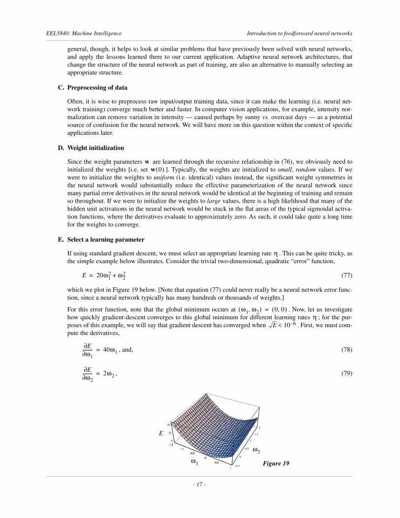
If using standard gradient descent, we must select an appropriate learning rate . This can be quite tricky, asthe simple example below illustrates. Consider the trivial two-dimensional, quadratic “error” function,

(77)

which we plot in Figure 19 below. [Note that equation (77) could never really be a neural network error func-tion, since a neural network typically has many hundreds or thousands of weights.]

For this error function, note that the global minimum occurs at . Now, let us investigatehow quickly gradient-descent converges to this global minimum for different learning rates ; for the pur-poses of this example, we will say that gradient descent has converged when . First, we must com-pute the derivatives,

, and, (78)

, (79)

ww 0( )

η

E 20ω12 ω2

2+=

-1.5-1

-0.5

0

0.5

1 -0.5

0

0.5

1

1.5

2

0

20

40

-1.5-1

-0.5

0

0.5

1Figure 19ω1

ω2

E

ω1 ω2,( ) 0 0,( )=η

E 10 6–<

E∂ω1∂

--------- 40ω1=

E∂ω2∂

--------- 2ω2=

- 17 -


so that the gradient-descent weight recursion in (76) is given by,

(80)

(81)

and similarly,

. (82)

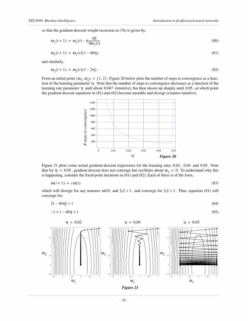
From an initial point , Figure 20 below plots the number of steps to convergence as a func-tion of the learning parameter . Note that the number of steps to convergence decreases as a function of thelearning rate parameter until about (intuitive), but then shoots up sharply until , at which pointthe gradient-descent equations in (81) and (82) become unstable and diverge (counter-intuitive).

Figure 21 plots some actual gradient-descent trajectories for the learning rates , and . Notethat for , gradient descent does not converge but oscillates about . To understand why thisis happening, consider the fixed-point iterations in (81) and (82). Each of these is of the form,

(83)

which will diverge for any nonzero and , and converge for . Thus, equation (81) willconverge for,

(84)

(85)

ω1 t 1+( ) ω1 t( ) η E∂ω1 t( )∂

----------------–=

ω1 t 1+( ) ω1 t( ) 1 40η–( )=

ω2 t 1+( ) ω2 t( ) 1 2η–( )=

ω1 ω2,( ) 1 2,( )=η

η 0.047 0.05

0 0.01 0.02 0.03 0.04 0.05

200

400

600

800

1000

1200

1400

Figure 20η

# st

eps

to c

onve

rgen

ce

0.02 0.04 0.05η 0.05= ω2 0=

-1.5 -1 -0.5 0 0.5 1

-0.5

0

0.5

1

1.5

2

-1.5 -1 -0.5 0 0.5 1

-0.5

0

0.5

1

1.5

2

-1.5 -1 -0.5 0 0.5 1

-0.5

0

0.5

1

1.5

2

ω1

ω2 ω2 ω2

ω1

Figure 21

ω1

η 0.02= η 0.04= η 0.05=

ω t 1+( ) cω t( )=

ω 0( ) c 1> c 1<

1 40η– 1<

1– 1 40η– 1< <

- 18 -


(86)

Since recursion (82) generates the weaker bound,

, (87)

the upper bound in (86) is controlling in that it determines the range of learning rates for which gradientdescent will converge in this example.

We make a few observations from this specific example: First, “long, steep-sided valleys” in the error surfacetypically cause slow convergence with a single learning rate, since gradient descent will converge quicklydown the steep valleys of the error surface, but will take a long time to travel along the shallow valley. Slowconvergence of gradient descent is largely why we will study more sophisticated learning algorithms, with defacto adaptive learning rates, later in this course. In this example, convergence along the axis is assuredfor larger ; however, the upper bound in (86) prevents us from using a (fixed) learning rate greater than orequal to . Second, Figure 20, although drawn specifically for this example, is generally reflective of gra-dient-descent convergence rates for more complex error surfaces as well. If the chosen learning rate is toosmall, convergence can take a very long time, while learning rates that are too large will cause gradientdescent to diverge. This is another reason to study more sophisticated algorithms — since selecting an appro-priate learning rate can be quite frustrating, algorithms that do not require such a selection have a real advan-tage. Finally, note that, in general, it is not possible to determine theoretical convergence bounds, such asthose in (86), for real neural networks and error functions. Only the very simple error surface in (77) allowedus to do that here.

F. Pattern vs. batch training

In pattern training, we compute the error and the gradient of the error for one input/output pattern at atime, and update weights based on that single training example (Section 5 describes pattern training). It isusually a good idea to randomize the order of training patterns in pattern training, so that the neural networkdoes not converge to a bad local minima or forget training examples early in the training.

In batch training, we compute the error and the gradient of the error for all training examples at once,and update the weights based on that aggregate error measure.

G. Good generalization

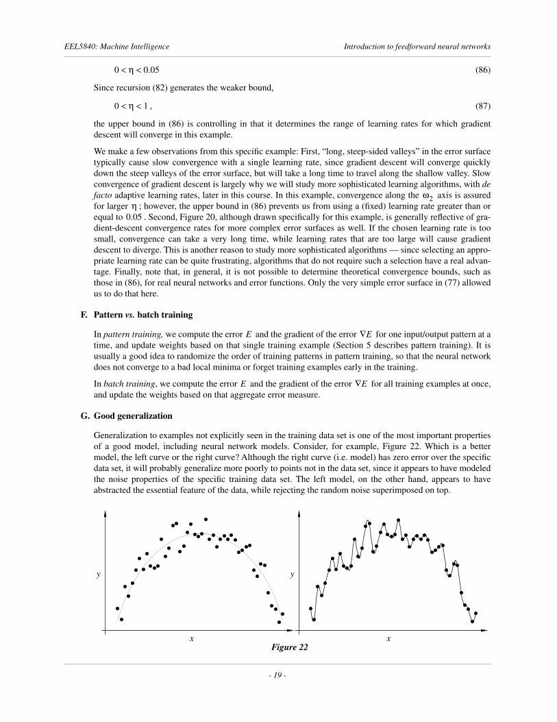
Generalization to examples not explicitly seen in the training data set is one of the most important propertiesof a good model, including neural network models. Consider, for example, Figure 22. Which is a bettermodel, the left curve or the right curve? Although the right curve (i.e. model) has zero error over the specificdata set, it will probably generalize more poorly to points not in the data set, since it appears to have modeledthe noise properties of the specific training data set. The left model, on the other hand, appears to haveabstracted the essential feature of the data, while rejecting the random noise superimposed on top.

0 η 0.05< <

0 η 1< <

ω2η

0.05

E E∇

E E∇

xFigure 22

y y

x

- 19 -


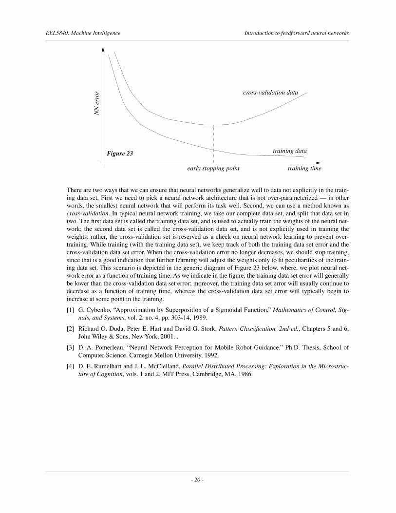
There are two ways that we can ensure that neural networks generalize well to data not explicitly in the train-ing data set. First we need to pick a neural network architecture that is not over-parameterized — in otherwords, the smallest neural network that will perform its task well. Second, we can use a method known ascross-validation. In typical neural network training, we take our complete data set, and split that data set intwo. The first data set is called the training data set, and is used to actually train the weights of the neural net-work; the second data set is called the cross-validation data set, and is not explicitly used in training theweights; rather, the cross-validation set is reserved as a check on neural network learning to prevent over-training. While training (with the training data set), we keep track of both the training data set error and thecross-validation data set error. When the cross-validation error no longer decreases, we should stop training,since that is a good indication that further learning will adjust the weights only to fit peculiarities of the train-ing data set. This scenario is depicted in the generic diagram of Figure 23 below, where, we plot neural net-work error as a function of training time. As we indicate in the figure, the training data set error will generallybe lower than the cross-validation data set error; moreover, the training data set error will usually continue todecrease as a function of training time, whereas the cross-validation data set error will typically begin toincrease at some point in the training.

[1] G. Cybenko, “Approximation by Superposition of a Sigmoidal Function,” Mathematics of Control, Sig-nals, and Systems, vol. 2, no. 4, pp. 303-14, 1989.

[2] Richard O. Duda, Peter E. Hart and David G. Stork, Pattern Classification, 2nd ed., Chapters 5 and 6,John Wiley & Sons, New York, 2001. .

[3] D. A. Pomerleau, “Neural Network Perception for Mobile Robot Guidance,” Ph.D. Thesis, School ofComputer Science, Carnegie Mellon University, 1992.

[4] D. E. Rumelhart and J. L. McClelland, Parallel Distributed Processing: Exploration in the Microstruc-ture of Cognition, vols. 1 and 2, MIT Press, Cambridge, MA, 1986.

Figure 23

NN

err

or

training time

cross-validation data

training data

early stopping point

- 20 -

Documents

EEL5840: Machine Intelligence Introduction to feedforward ... · train artiﬁcial neural networks to model input/output data; that is, how learning occurs in artiﬁcial neural net-works