Journal Pre-proof

EEG Sleep Stages Identification Based on Weighted UndirectedComplex Networks

Mohammed Diykh , Yan Li , Shahab Abdulla

PII: S0169-2607(18)31325-7DOI: https://doi.org/10.1016/j.cmpb.2019.105116Reference: COMM 105116

To appear in: Computer Methods and Programs in Biomedicine

Received date: 10 September 2018Revised date: 14 September 2019Accepted date: 2 October 2019

Please cite this article as: Mohammed Diykh , Yan Li , Shahab Abdulla , EEG Sleep Stages Iden-tification Based on Weighted Undirected Complex Networks, Computer Methods and Programs inBiomedicine (2019), doi: https://doi.org/10.1016/j.cmpb.2019.105116

This is a PDF file of an article that has undergone enhancements after acceptance, such as the additionof a cover page and metadata, and formatting for readability, but it is not yet the definitive version ofrecord. This version will undergo additional copyediting, typesetting and review before it is publishedin its final form, but we are providing this version to give early visibility of the article. Please note that,during the production process, errors may be discovered which could affect the content, and all legaldisclaimers that apply to the journal pertain.

© 2019 Published by Elsevier B.V.

1

Highlights

A statistical model and weighted networks are used to identify EEG sleep stages.

The proposed system requires one input the EEG signals without pre-processing.

The results showed that the network’s characteristics vary with their sleep stages.

Each sleep stage is best represented using the key features of their networks.

2

EEG Sleep Stages Identification Based on Weighted Undirected Complex

Networks

Mohammed Diykh11,a,c ,

Yan Lia, Shahab Abdulla

b

aSchool of Agricultural, Computational and Environmental Sciences, University of Southern Queensland,

Australia bOpen Access College , University of Southern Queensland, Australia

cUniversity of Thi-Qar, College of Education for Pure Science, Iraq

{Mohammed.Diykh; Yan.Li; Shahab.Abdulla }@usq.edu.au

Abstract:

Background and Objective: Sleep scoring is important in sleep research because any errors in the scoring of the

patient’s sleep electroencephalography (EEG) recordings can cause serious problems such as incorrect diagnosis,

medication errors, and misinterpretations of patient’s EEG recordings. The aim of this research is to develop a new

automatic method for EEG sleep stages classification based on a statistical model and weighted brain networks.

Methods: each EEG segment is partitioned into a number of blocks using a sliding window technique. A set of

statistical features are extracted from each block. As a result, a vector of features is obtained to represent each EEG

segment. Then, the vector of features is mapped into a weighted undirected network. Different structural and spectral

attributes of the networks are extracted and forwarded to a least square support vector machine (LS-SVM) classifier. At

the same time the network’s attributes are also thoroughly investigated. It is found that the network’s characteristics

vary with their sleep stages. Each sleep stage is best represented using the key features of their networks. Results: In

this paper, the proposed method is evaluated using two datasets acquired from different channels of EEG (Pz-Oz and

C3-A2) according to the R&K and the AASM without pre-processing the original EEG data. The obtained results by

the LS-SVM are compared with those by Naïve, k-nearest and a multi-class-SVM. The proposed method is also

compared with other benchmark sleep stages classification methods. The comparison results demonstrate that the

proposed method has an advantage in scoring sleep stages based on single channel EEG signals. Conclusions: An

average accuracy of 96.74% is obtained with the C3-A2 channel according to the AASM standard, and 96% with the

Pz-Oz channel based on the R&K standard.

Keywords: Sleep stages, weighted networks, statistical model, EEG single channel.

1. Introduction

Sleep is a dynamic process involved in two main stages: rapid eye movement (REM) and non-rapid eye movement

(NREM) [5, 14, 18, 34, 69]. The later includes three stages of Stage 1 (S1), Stage 2 (S2), and slow wave sleep (SWS).

These individual sleep stages are connected through different physiological and neuronal characteristics that are used in

sleep identification by experts and researchers. The process of discriminating sleep stages visually is called sleep

scoring or sleep staging. Normally, it is carried out visually by experts according to either Rechtschaffen or Kales

(R&K) [50] or the American Academy of Sleep Medicine (AASM) [9] guidelines. Based on the R&K guidelines, sleep

recordings are divided into seven different stages namely: Awake (AWA), S1, S2, S3, S4, REM and movement time.

Although, for the past 40 years, the R&K guidelines have been used as the standard for sleep scoring. It has received

1 Corresponding author: Mohammed Diykh

3

many criticisms for leaving too much room for subjective interpretations, for which a wide variability in the visual

evaluation of sleep stages would occur. In 2007, the AASM guidelines were modified to address some revealed issues

in the R&K. In the AASM guidelines the allocated time for S1 and SWS were changed, and a minimum of three EEG

derivations including F4-M1, C4- M1, and O2-M1 from the frontal, central, and occipital regions must be recorded. The

AASM combines S3 and S4 into one stage [9], and considers the body movement as one of the sleep stages.

Although the visual inspection for sleep staging remains the standard method for a number of decades, there has been a

surge in demand for developing automatic sleep scorings [10, 13] due to the drawbacks of the manual inspection, such

as being subjective and time consuming. Most of automatic sleep staging approaches have been carried out in two

phases: (i) to eliminate the undesired information and to extract the key features, (ii) to classify the extracted features

for distinguishing the sleep stages [15, 5]. The majority of sleep staging research has been carried out by means of

analysing electroencephalography (EEG) signals, for some cases electromyography (EMG) or a combination of the

EEG, and Electrooculography (EOG) recordings were used for identifying specific sleep stages [3, 6, 53, 52]. From the

literature, the automatic sleep stages classification methods were mainly developed depending on analysing EEG

signals recorded from a single EEG channel [15, 16, 17, 24, 49] instead of multiple-channels [42]. Various types of

approaches from time domain [44], frequency domain [59, 9], time-frequency domain [16], and graphs domain [1, 14,

15, 16, 72] were utilized for extracting the key features from EEG signals.

The wavelet transform, and fast Fourier transform have been commonly utilized in sleep research compared with their

counterparts in time domain [24]. Peker [49] suggested a sleep classification model based on frequency domain where a

dual wavelet transform was used to extract features from EEG data. Gao et al. [19] proposed a multi-classifiers system

for sleep stages classification based on Fast Fourier transform with a hamming window length equal to the EEG

segment length. da Silveira et al. [12] applied a normalized wavelet transform for decomposing EEG signals into

different frequency bands. The statistical parameters were obtained from each decomposing level. The extracted

parameters were then fed to a random forest classifier. Ebrahimi et al. [17] applied a wavelet packet tree of seven levels

to break down an EEG signal into five different bands. A set of statistical features was extracted from the coefficients of

those bands and then was used to identify the EEG sleep stages. Kayikcioglu [28] classified a single channel EEG

signal based on auto-regressive coefficients. The single EEG channel was normalized and then filtered using a

Butterworth band pass filtered. Liang et al. [41] used a multiscale entropy and an autoregressive model for features

extraction. A linear discrimination analysis was used to classify the extracted features.

Nonlinear features have been investigated by many researchers. Acharya et al. [3] compared and analysed 29 nonlinear

measures such as high order spectra and recurrence quantification analysis to identify the sleep stages. In that study, the

extracted nonlinear features were ranked based on f-value. Acharya et al. [2] also used a nonlinear technique based on

high order spectra (HOS). In that study, Bispectrum and bicoherence plots were utilized to extract four HOS features to

classify EEG sleep stages. Lee et al. [35] applied a nonlinear approach based on detrended fluctuation analysis to study

and identify the EEG sleep stages. Zhou et al. [70] used detrended fluctuation analysis to detect apnea using EEG

signals.

More recently, Diykh et al. [15, 14], applied the concept of complex networks combined with a statistical model to

classify single EEG channel signals for six sleep stages. Zheu et al. [72] discriminated the sleep stages based on a

visibility graph algorithm. Each EEG segment was transferred into horizontal and vertical visibility graphs. Seven

features were extracted and then fed to a SVM classifier. Liu et al. [42] propounded a multi-domain approach for

4

identifying the EEG sleep stages. Fifteen features were extracted using different techniques including: visibility graphs,

frequency domain, detrened fluctuation analysis, natural graph and non-linear analysis. Rodríguez-Sotelo et al. [54]

proposed entropy metrics extracted from an EEG signal. The resulting features vector was optimized by a

method and fed to a J-means clustering algorithm. Bajaj et al. [6] classified the EEG sleep stages based on time

frequency images (TFIs). TFIs were obtained using a time frequency representation based on Winger-Ville distribution.

The statistical features of the histogram of each TFI were utilized to classify the EEG sleep stages. Xia et al. [67]

identified the sleep stages using EOG signals. A deep belief network blended with a hidden Markov model was

employed to classify each EOG segment into one of these sleep stages. Mousavi et al. [47] developed a methodology

based on conventional neural networks to classify EEG sleep stages. Jiang et al. [25] considered multi-channels signals

technique to identify EEG sleep stages. Each single EEG channel was segmented into small intervals of 30 second.

Covariance matrices were used to extract the most representative features from EEG segments. Two machine learning

algorithms were employed to classify the extracted features. Then a HMM- based refinement process was adopted to

optimise the classification results. Jiang et al. [26] employed a multi-decomposition approach-based features selection

to categorise EEG sleep stages. Ghasemzadeh et al. [20] proposed a logistic smooth transition autoregressive model

(LSTAR)to investigate EEG sleep signals. Each 30 EEG segment was decomposed into several bands using a double-

density dual-tree discrete wavelet transform. Then the LSTAR with a tensor locality preserving projection was utilised

to pull out and select a set of EEG features. Abdulla et al. [1] applied a correlation graphs similarity concept to analyse

EEG sleep signals. in that study, an ensemble machine learning algorithm was developed to classify graph features.

EEG signals exhibit nonlinear behaviours. One of the effective non-linear methods is complex networks. Based on our

previous research [14, 15], we found that complex networks yielded promising results in EEG signals classification. In

this paper, we employed a weighted complex network to further improve the performance. Based on the obtained

results, it was found that the weighted complex networks were capable to identify EEG patterns for sleep staging. In

this paper, each EEG segment is partitioned into smaller blocks using a sliding window technique. Total 12 statistical

features are extracted from each block and are put in one vector to represent a 30 second EEG segment. The vector of

the extracted features is then mapped as a weighted undirected complex network. The spectral and structural

characteristics of the networks are extracted from each network. Then, extensive simulations and experiments are

carried out to analyse the attributes of the networks for sleep stages classification, and to determine the effective

characteristics of the network’s to represent each sleep stage. A least square support vector machine (LS-SVM)

classifier is used to identify the sleep stages. The results obtained by the LS-SVM are compared with those from Naïve

Bayes, k-nearest, a multi-class-SVM for the performance evaluation. The performance of the proposed method is also

compared with other previous research work. Our findings demonstrated that each sleep stages can be categorized with

a specific set of network features.

The paper is organised as follows: In Section 2, the information regarding to the data used in this paper is presented.

Section 3 describes the methodology of the proposed method and the relevant fundamentals. Section 4 presents the

experimental and simulation results. In Section 5, the results and findings of this paper are discussed. In Section 6, the

conclusions of the paper are drowned.

2. EEG Data

5

In this work, two publicly available datasets were used to evaluate the proposed method in EEG sleep stages

classification. The datasets were acquired from two different channels and scored by either the R&K or the AASM

guidelines. The following section gives a brief explanation for the two datasets.

2.1. ISRUC-Sleep database

One set of EEG data used in this paper is from ISRUC-Sleep database acquired at the Hospital of Coimbra University

during 2009-2013 [32, 50, 31]. It contains three sub-groups. Each sub-group comprises different subjects, including

healthy subjects, subjects with sleep disorders and subjects under effects of medications. The recorded data for those

sub-groups were gathered from 8, 10 and 100 participants respectively. Each recording contains 19 channels. The EEG,

EMG and EOG signals were sampled at 200 Hz, and they were stored as European Data Format (EDF) files. The EEG

signal from C3-A2 channel is used in this paper as it is proven for giving better classification results [32]. The

recordings were scored by two experts based on the AASM rules. All the recordings were partitioned into 30 second

segments and each segment was assigned into one of the five sleep stages in accordance with the AASM guidelines [9].

The dataset is publically available for sleep research. The EEG recordings from 18 subjects of subject 1 to subject 18

were used in this paper. Their demography information was as follows: 15 males and 4 females, aged between 22-76,

with a weight from 41 kg to 110 kg and height from 68cm to 178 cm. Table 1 presents the distribution of the sleep

stages used which were carried out by the two experts.

2.2. Sleep-EDF database

Another set of the EEG data used in this paper was obtained from PhysioNet [22, 30, 46, 64, 29]. The online Sleep-

EDF datasets (expanded) were used. In this database, 61 EEG recordings were collected from two studies. 13 subjects

were used for simulations in this paper including SC4001E0, SC4011E0, SC4012E0, SC4021E0, SC4022E0,

SC4031E0, SC4032E0, SC4041E0, SC4042E0, SC4051E0, SC4002E0, SC4061E0 and SC4062E0.The

polysmnographic includes two EEG channels recorded from Fpz-Cz and Pz-Oz, one EOG, one EMG, Resporonasal,

EMGSubmenta, Tempbody, and Eventmarker. The datasets were acquired from different volunteers in 1987-1994 from

Caucasian males and female. All the recordings were stored in EDF format. The original EEG signals were sampled at

100 Hz. They were scored with segments of 30 second (3000 data points) based on the R&K criteria [43]. The segments

were labelled as AWA, S1, S2, S3, S4, REM MVT (movement time), and UNS (unknown state). Table 2 shows the

number of segments that were used in this study.

Table 1

Distribution of the sleep stages in the ISRUC dataset

Sleep stage AWA S1 S2 SWS REM Total number of epochs

No. of epochs 5103 2083 4364 2909 1767 16226

Table 2

Distribution of the sleep stages in the EDF database

Sleep stage AWA S1 S2 S3 S4 REM Total number of epochs

No. of epochs 8055 604 3621 672 627 1609 15188

6

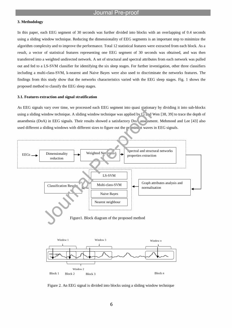
3. Methodology

In this paper, each EEG segment of 30 seconds was further divided into blocks with an overlapping of 0.4 seconds

using a sliding window technique. Reducing the dimensionality of EEG segments is an important step to minimize the

algorithm complexity and to improve the performance. Total 12 statistical features were extracted from each block. As a

result, a vector of statistical features representing one EEG segment of 30 seconds was obtained, and was then

transferred into a weighted undirected network. A set of structural and spectral attributes from each network was pulled

out and fed to a LS-SVM classifier for identifying the six sleep stages. For further investigation, other three classifiers

including a multi-class-SVM, k-nearest and Naive Bayes were also used to discriminate the networks features. The

findings from this study show that the networks characteristics varied with the EEG sleep stages. Fig. 1 shows the

proposed method to classify the EEG sleep stages.

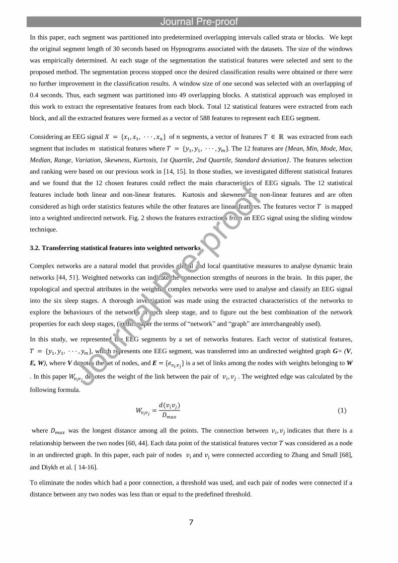
3.1. Features extraction and signal stratification

As EEG signals vary over time, we processed each EEG segment into quasi stationary by dividing it into sub-blocks

using a sliding window technique. A sliding window technique was applied by Li and Wen [38, 39] to trace the depth of

anaesthesia (DoA) in EEG signals. Their results showed a satisfactory DoA assessment. Mehmood and Lee [43] also

used different a sliding windows with different sizes to figure out the prominent waves in EEG signals.

Window 1

Window 2

Window 3

EEG signal

Window n

Figure 2. An EEG signal is divided into blocks using a sliding window technique

Block 1 Block 2 Block 3 Block n

Dimensionality

reduction

Spectral and structural networks

properties extraction

Weighted Networks EEGs

Classification Results

LS-SVM

Multi-class-SVM

Naive Bayes

Nearest neighbour

Graph attributes analysis and

normalisation

Figure1. Block diagram of the proposed method

7

In this paper, each segment was partitioned into predetermined overlapping intervals called strata or blocks. We kept

the original segment length of 30 seconds based on Hypnograms associated with the datasets. The size of the windows

was empirically determined. At each stage of the segmentation the statistical features were selected and sent to the

proposed method. The segmentation process stopped once the desired classification results were obtained or there were

no further improvement in the classification results. A window size of one second was selected with an overlapping of

0.4 seconds. Thus, each segment was partitioned into 49 overlapping blocks. A statistical approach was employed in

this work to extract the representative features from each block. Total 12 statistical features were extracted from each

block, and all the extracted features were formed as a vector of 588 features to represent each EEG segment.

Considering an EEG signal of segments, a vector of features was extracted from each

segment that includes statistical features where . The 12 features are {Mean, Min, Mode, Max,

Median, Range, Variation, Skewness, Kurtosis, 1st Quartile, 2nd Quartile, Standard deviation}. The features selection

and ranking were based on our previous work in [14, 15]. In those studies, we investigated different statistical features

and we found that the 12 chosen features could reflect the main characteristics of EEG signals. The 12 statistical

features include both linear and non-linear features. Kurtosis and skewness are non-linear features and are often

considered as high order statistics features while the other features are linear features. The features vector is mapped

into a weighted undirected network. Fig. 2 shows the features extractions from an EEG signal using the sliding window

technique.

3.2. Transferring statistical features into weighted networks

Complex networks are a natural model that provides global and local quantitative measures to analyse dynamic brain

networks [44, 55]. Weighted networks can indicate the connection strengths of neurons in the brain. In this paper, the

topological and spectral attributes in the weighted complex networks were used to analyse and classify an EEG signal

into the six sleep stages. A thorough investigation was made using the extracted characteristics of the networks to

explore the behaviours of the networks at each sleep stage, and to figure out the best combination of the network

properties for each sleep stages, (in this paper the terms of “network” and “graph” are interchangeably used).

In this study, we represented the EEG segments by a set of networks features. Each vector of statistical features,

, which represents one EEG segment, was transferred into an undirected weighted graph G= (V,

E, W), where V denotes the set of nodes, and is a set of links among the nodes with weights belonging to W

. In this paper denotes the weight of the link between the pair of . The weighted edge was calculated by the

following formula.

where was the longest distance among all the points. The connection between indicates that there is a

relationship between the two nodes [60, 44]. Each data point of the statistical features vector was considered as a node

in an undirected graph. In this paper, each pair of nodes and were connected according to Zhang and Small [68],

and Diykh et al. [ 14-16].

To eliminate the nodes which had a poor connection, a threshold was used, and each pair of nodes were connected if a

distance between any two nodes was less than or equal to the predefined threshold.

8

{

here is a predefined threshold.

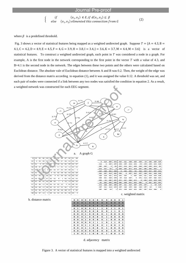
Fig. 3 shows a vector of statistical features being mapped as a weighted undirected graph. Suppose

is a vector of

statistical features. To construct a weighted undirected graph, each point in was considered a node in a graph. For

example, A is the first node in the network corresponding to the first point in the vector with a value of 4.3, and

B=4.1 is the second node in the network. The edges between these two points and the others were calculated based on

Euclidean distance. The absolute vale of Euclidean distance between A and B was 0.2. Then, the weight of the edge was

derived from the distance matrix according to equation (1), and it was assigned the value 0.12. A threshold was set, and

each pair of nodes were connected if a link between any two nodes was satisfied the condition in equation 2. As a result,

a weighted network was constructed for each EEG segment.

c. weighted matrix

b. distance matrix

d. adjacency matrix

Figure 3. A vector of statistical features is mapped into a weighted undirected

graph

K

J H I

F

C

E

N

G

0.57

A

D B

a. A graph G

M

0.57

0.64

0.71

0.78 0.92 0.85

1

0.64 0.57

0.71

0.57

0.71

0.64

0.86

0.85

0.92 0.72

0.64 0.57

9

The adjacency matrix A of graph G was calculated for all V to describe the network nodes connection. The adjacent

matrix of an undirected weighted graph is symmetric, i.e. A ( = A (

{

The graph Laplacian matrix was also calculated using the formula of =D-A where D is a diagonal degree matrix, and

is the adjacency matrix of graph G [7]. Matrix D was formed by the degree of each node. The elements of the

Laplacian matrix were produced using the following formula:

( ) {

where denotes the degree of the node.

From Fig. 3 we can notice that, there is a node, such as {C} without any connections with other nodes in the network.

This node is isolated points in the network. The number of isolated points in the network was also used as an important

feature to distinguish the sleep stages. In this paper all the graphs have been constructed with the same number of

nodes.

3.2.1. Structural and spectral network features

A set of structural and spectral graph properties were calculated in this paper to represent EEG data [11, 37, 36, 56, 51,

68]. The structural and spectral network attributes can capture the local relationships among nodes. Based on recent

studies of analysing brain networks, structural and spectral networks features allow to go through a deeper investigation

towards knowledge extraction among brain regions. Our research showed how a combination of structural and spectral

attributes of weighted networks could reflect EEG signal patterns.

Average degree

The average degree is defined as the number of edges linking a node in a graph with other nodes. The average degree

of a network is the average of the node degrees for all the nodes in the network i.e.

∑

where n is the number of nodes in a network, is the average degree of the network, and denotes to the

degree of node

Average Clustering Coefficient

10

Clustering coefficient is commonly used to compute the similarity among nodes based on the fraction of triangles. The

clustering coefficient for a node in a graph G is defined as

, where is the number of the actual links

between with its neighbours, and is the number of the neighbours of .

The clustering coefficient of a graph is the average of the clustering coefficients of all the nodes.

∑

where is the number of nodes in the network and is the clustering coefficient for node .

Shortest path

Let L be the average of the shortest path length between any pair of the nodes. The length represents the number of

steps from node to node . A low number of L indicates that the network has a high level of connections and

communication efficiency. This attribute is used to detect the sleep stages.

The number of the isolated points

The number of the isolated points are defined as the number of nodes in a network that have a zero degree. In this

paper, the number of the isolated points in a network is used as a feature to differentiate the sleep stages.

The maximum eigenvalue

The eigenvalues of a graph are sorted in a descending order from the smallest to the largest. The graph eigenvalues can

represent the most important attributes in a graph. The largest value is selected as a representative for each EEG

segment.

The second largest eigenvalue

The second largest eigenvalue of a graph G is also used as a key network characteristic.

Spectral radius: The spectral radius is defined as the largest magnitude eigenvalue for a graph. Let | > |

, be the distinct eigenvalues of graph G, sorted by their magnitudes. The spectral radius of the

graph , is defined as =|

Energy of a graph

The energy of a graph is the squared sum of the eigenvalues in a graph. More formally, the energy of a graph G is

defined as

∑

3.3. Classification

The network’s attributes were forwarded to the LS-SVM classifier and also to multi-class-SVM, k-nearest and Naive

Bayes for performance comparison. This section briefly introduce those classifiers.

3.3.1. Least Square Support Vector Machine (LS-SVM)

The least square support vector machine (LS-SVM) was first developed by Suyken and Vandewalle [61, 62] as a

modified version of the original support vector machine [5, 6]. It was used by Siuly et al. [38] for the motor image

classification, also by Al Ghayab et al. [4] for detecting the epileptic EEG signals.

11

Two main parameters, should be carefully tuned in the LS-SVM for obtaining the desired classification

results. The two parameters can positively or negatively affect the performance of the proposed method. The LS-SVM

was employed to classify different pairs of sleep stages, the values of were empirically set during the training

set. The best performance for the proposed method for identifying the awake and sleep (AWA-Sleep) pair was obtained

when . For the other pairs of (S3, S4), ((S1, S2), SWS), (S1, S2), (S1, REM), (AWA-REM), the best

recorded results were achieved when the values of were set as (10, 1), (2, 1), (10, 10) (10, 10), (1, 1)

respectively.

3.3.2. Multi-class SVM classification

The SVM was originally a binary classification method developed by Vapink and colleagues at Bell laboratories [8, 39,

47]. It was then developed for the multi-class classification [45]. However, it is still an ongoing challenge to use the

multi-class SVM for the classification task. For the sleep stages classification, it is required to discriminate each

individual sleep stage from the total six sleep stages of (AWA, S1, S2, S3, S4 and REM). To target the multi-class

problem, a common approach to use the SVMs is to decompose the multi-class problems into several binary problems.

The most popular strategies are one-against-all (OAA) and one-against-one (OAO) [37]. The OAA is a simple method

for the multi-class classification, which consists of a binary SVM to recognise each class from other classes. The OAO

requires to train two-way classifiers for all possible pairs of classes. Thus, the OAA needs k (k-1)/2 binary SVMs, while

the OAO requires k binary SVMs, where k is the number of the classes. In this work, the OAO ( multi-class- SVM) is

used as a classifier to discriminate EEG sleep stages.

3.3.3. K-nearest neighbour classifier

The k-nearest neighbour is one of the simplest and widely used classifiers in pattern recognition [66]. It uses Euclidian

distance to compute the similarity between the training case and the case in the classification record. A record is

maintained in order to store the classification performance and similarity results. In order to classify a sample, the

similarities with k-nearest neighbours are computed and the class corresponding to the maximum number of votes is

assigned as the output class of the sample.

3.3.4. Naive Bayes

Naive Bayes is frequently used in pattern recognition. It works based on the applications of Bayes' rules and posterior

hypothesis. Naive Bayes provides a simpler approach based on the probabilistic knowledge to precisely predict the

classes. This algorithm assumes that each attribute influences differently on a given class. Assume Y= {g1, g2, ……gn}

is a sample set that includes a set of n attributes. Let H represents the hypothesis that each set of Y belongs to a specific

class. In Naive Bayes rules, we considered Y the evidence and seek to assign each attribute in Y to the highest posteriori

probability class [27]. In this paper, Naive Bayes is also employed to classify the characteristics of the complex

networks.

3.4. Performance Evaluation

Four measures including K-cross validation, sensitivity, kappa coefficient, and confusion matrix are utilized to assess

and examine the performance of the proposed method [14, 58].

3.4.1.K-fold cross validation: it is a popular approach to assess the performance of a classification algorithm. It is used

to estimate the quality of a classification method by dividing the number of correctly classified results by the total of the

cases. The datasets in Section 2 were divided into k exclusive subsets in an equal size. One subset was considered as the

testing set, while others were used as the training sets. All the subsets were alternatively used and the classification

12

accuracies were reported. In this work, the 10-fold cross-validation is used. The average of the overall results for the

subset testings is computed.

Performance=

∑

where is the accuracy for (k=1, 2,….10).

3.4.2. Sensitivity: a statistical measure by which the performance of a classification algorithm is assessed by computing

the proportion of the actual positive classification. It is defined as

Sensitivity =

where TP is the number of the positive classification for all the subset testings, FN is the number of incorrect

classification for the subsets.

3.4.3. Confusion matrix: it is a statistical method in which the performance of an algorithm is described by means of

comparing the actual and predication classification results by the algorithm. In this paper, the actual predication is from

the experts scoring while the predication is by the proposed method.

Classification accuracy: it is defined by the number of the samples correctly classified divided by the total number of

the samples.

Accuracy =

where

3.4.4. Kappa coefficient: is a statistical measure that evaluates the agreement between two classification results, those

by the proposed method and the expert.

Kappa coefficient =

where,

(

) (

)

3.4.5. Receiver operating characteristics (ROC): it is a significant tool to evaluate the quality of classification

algorithms by comparing sensitivity against specificity across a range of instances. It is represented by a graph in which

the false positive rate is plotted on x-axis while the true positive rate is plotted on y-axis.

4. Experimental results and complex network analysis

A series of experiments were made to evaluate the performances of the proposed method. The datasets described in

Section 2 were used in the experiments. To identify the sleep stages through complex networks, the behaviours of the

networks were analysed. It was found that each sleep stages could be categorized with a specific set of graph

characteristics. All the experimental results were obtained in a MATLAB 2015b environment on a computer with the

following settings: 3.40 GHz Intel(R) core(TM) i7 CPU processor machine, and 8.00GB RAM. The testing and training

phases were performed by means of 10-fold cross validation method.

13

4.1. Significant characteristics of network properties and networks behaviour analysis

EEG signals are often contaminated with noise and non-stationary [53, 46]. Inappropriate features could not result in the

desirable results for EEG sleep stages classification. We conducted extensive experiments to investigate and select

suitable features to represent individual sleep stages. We investigated the effectiveness of each graph attributes on sleep

stages classification and its relationship with each stage. It was found that a sleep stage was better classified with

separated

network attributes. For example, the shortest path can be used as one of the important network characteristics to identify

the AWA stages while it has a little influence on the recognition of S1 or S2.

Table 3 shows the network features best representing each sleep stages based on the experimental results. The network

features for each sleep stages in Table 3 were selected based on the binary classification results during the training

stage. The classifiers were trained with balanced data (50% of EEG epochs were used for the training and the other

50% of EEG epochs were used for the testing).The results in Table 3 were obtained through extensive experiments. An

equal number of segments were used for each pair of sleep stages to avoid inconsistency. The network’s features in

Section 3.1 were extracted and the LS-SVM was also employed to classify each pair of the sleep stages. The parameters

of the LS-SVM were selected during the simulation session. As a result, for identifying {AWA, Sleep}, the LS-SVM

parameters were set as , while the other pairs of {S3, S4}, {(S1, S2), SWS}, {S1, S2}, {S1, REM},

{AWA, REM}, the best classification results were achieved when the values of were set as (10, 1), (2, 1), (10,

10) (10, 10) and (1, 1) respectively. At each iteration, different graph attributes were used and the accuracy of the LS-

SVM classifier was recorded.

Once the accuracy started to increase, the optimum features set was updated. The procedure was applied for each pair of

the sleep stages to discover the best graph attributes representing their sleep stages. The obtained results revealed that

not all the sleep stages could be represented with the same network features. For example, the features of {average

degree,

Table 3

The selected weighted network features for each sleep stage pairs after the training phase

Sleep stages network characteristics

{AWA, Sleep} average degree, average of clustering coefficient , spectrum radius, shortest path, graph energy

{AWA, REM} average degree, average of clustering coefficient, graph energy, spectrum radius, shortest path

{S1, REM} energy of graph, average of clustering coefficient, maximum eigenvalue, average degree, second

maximum eigenvalue

{S1, S2} average degree, average of clustering coefficient maximum eigenvalues and second maximum eigenvalue

{(S1,S2), SWS} average degree, average of clustering coefficient, maximum eigenvalues and second maximum

eigenvalue, energy of graph and number of isolated points

{S3, S4} average degree, average of clustering coefficient, maximum eigenvalue, shortest path, spectrum radius

and number of isolated points

14

average of clustering coefficient, spectrum radius, shortest path, graph energy} were used to identify the pair {AWA,

Sleep}. That means, using the same features to classify all the sleep stages could not give the promising results. One of

the interesting results, we found in this paper is that the network’s characteristics vary with their sleep stages.

During the experiment, it was noticed that some attributes of the networks, such as clustering coefficients and degree

distribution, were more significant compared to other network attributes to recognize the sleep stages. To investigate the

effectiveness of the attributes on the identification of sleep stages, box plots were used. In each box plot, the upper part

of the box denotes the 75% percentile, the lowest part of the box represents the 25% percentile and the line on the

middle refers to the median 50% percentile (also called centre). The highest and lowest values are marked by the lines

extending from the top to the bottom of the box.

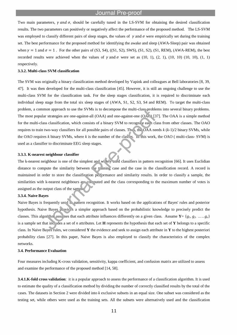
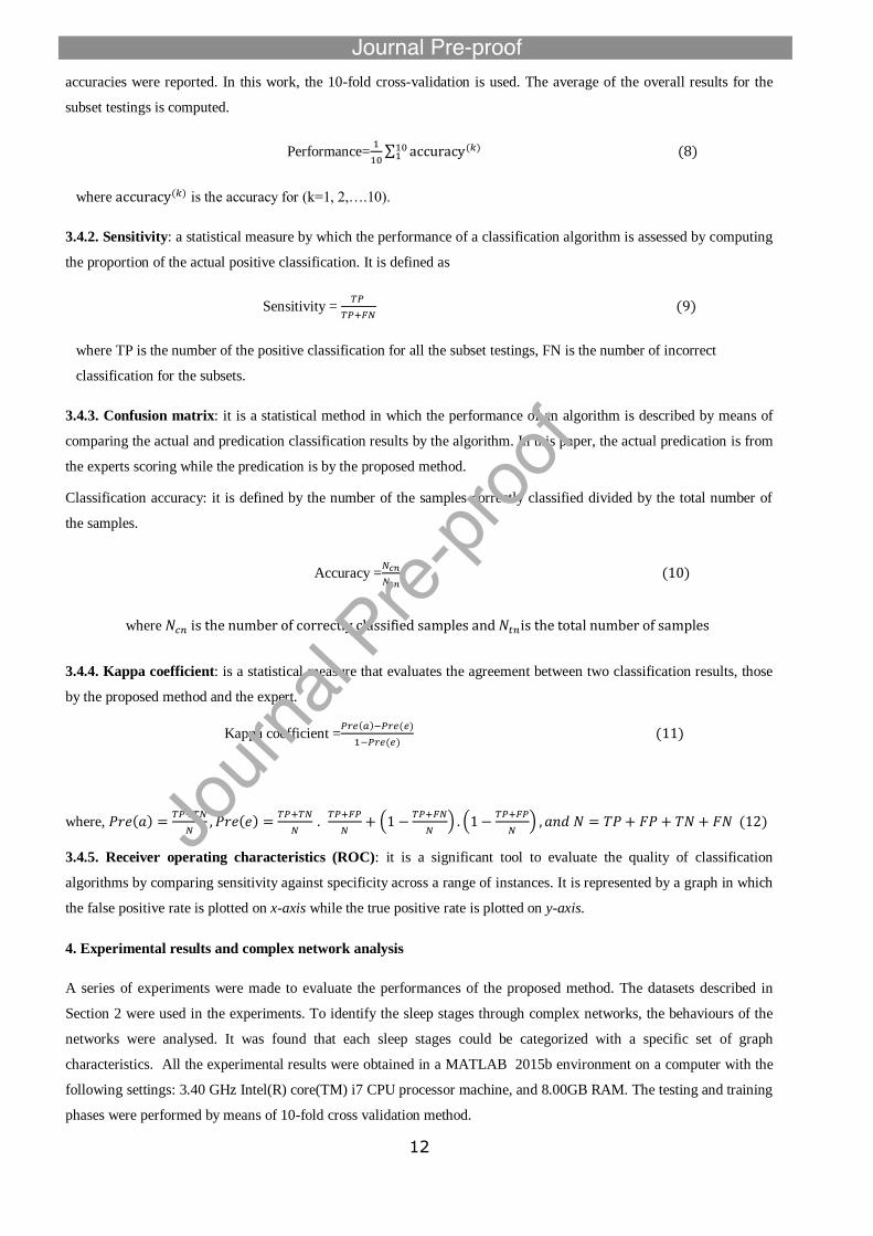
From Figs. 4 and 5 we can see that the clustering coefficients, and degree distribution can be used as the key attributes

to differentiate the sleep stages. The statistical mean degree of the clustering coefficients, and the degree distribution

that are associated with the five sleep stages are shown in Fig. 4 and Fig. 5. The results in Figs. 4 and 5 support the

research findings in Table 3 in which the clustering coefficients and the degree distribution are the key features to

represent all the sleep stages. A statistical analysis for all the network’s characteristics was also conducted to evaluate

the differences of the networks attributes among the individual sleep stage pairs using Wilcoxon rank sum test. It was

found that the average of cluster coefficients of the networks changed over the sleep stages transition, and the links of

networks were significantly stronger during the AWA, and the light sleep stage compared with the REM and SWS

stages. The results in Tables 4 and 5 indicate that the attributes of {Cluster coefficient, graph energy, spectrum radius,

shortest path, graph energy} for the {AWA, Sleep} stage pair were different from those of other pairs. These networks

characterises can be used to distinguish between the pairs of {AWA, Sleep} and {AWA, REM}.

Table 6 depicts another example. It presents a set of networks characteristics of {cluster coefficients, graph energy,

spectrum radius, maximum eigenvalue, second maximum eigenvalue} that indicate the significant differences between

the pairs of {S1, REM}. Table 7 shows p-values for 4-state, 5-state and 6-state sleep stages. The results in Tables 4, 5,

6 and 7 show that each pair of the sleep stages can be represented by a specific set of the network characteristics. The

same procedure was conducted for all the sleep stage pairs to study the network behaviours. Such findings are

significant at ( in terms of statistics.

Table 4

Differences in networks attributes for separating {AWA, Sleep}

40

50

60

70

80

90

100

110

120

130

AWA S1 S2 SWS REM

Av

era

ge

de

gre

e

EEG signals groups

Figure 4. Box plot of the average degree Figure 5. Box plot of the clustering coefficients

0.2

0.3

0.4

0.5

0.6

0.7

0.8

0.9

AWA S1 S2 SWS REM

Clu

steri

ng c

oeff

icie

nts

EEG signals groups

15

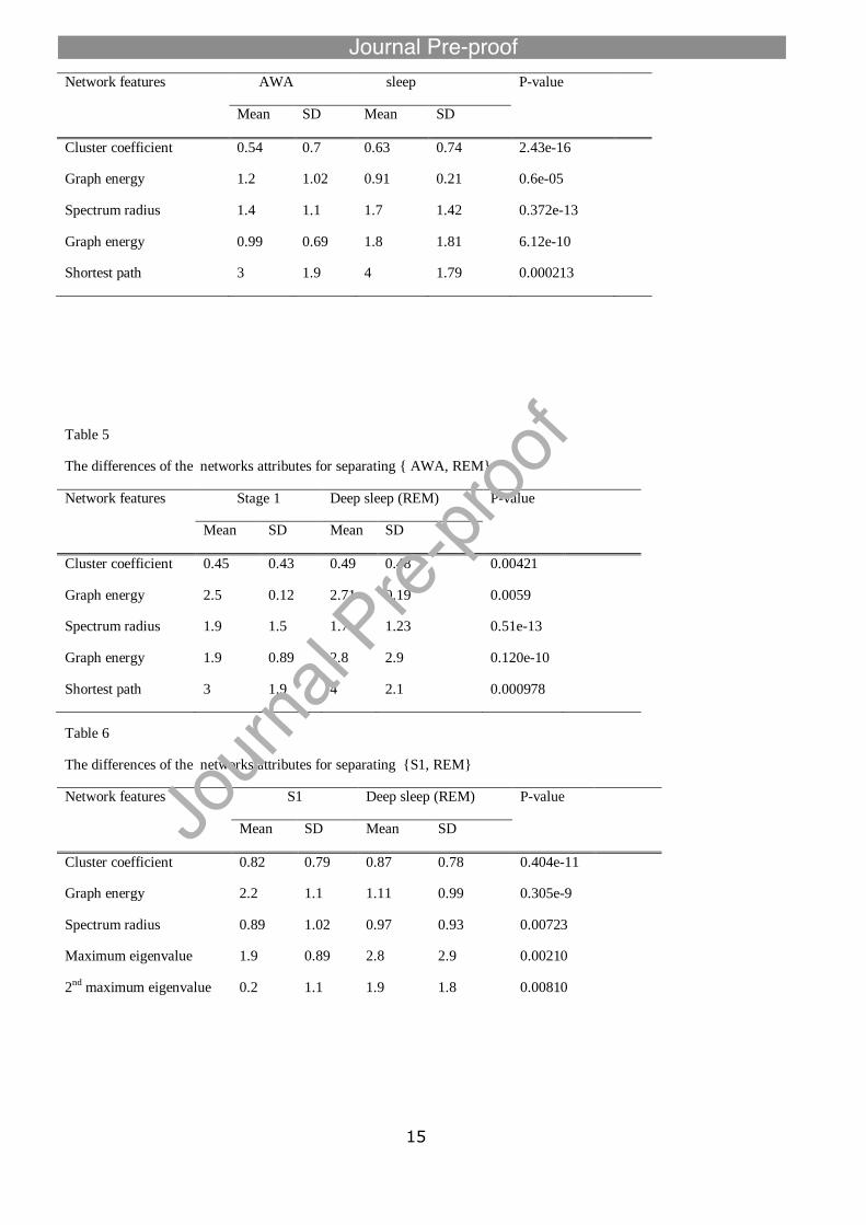
Network features AWA sleep P-value

Mean SD Mean SD

Cluster coefficient 0.54 0.7 0.63 0.74 2.43e-16

Graph energy 1.2 1.02 0.91 0.21 0.6e-05

Spectrum radius 1.4 1.1 1.7 1.42 0.372e-13

Graph energy 0.99 0.69 1.8 1.81 6.12e-10

Shortest path 3 1.9 4 1.79 0.000213

Table 5

The differences of the networks attributes for separating { AWA, REM}

Network features Stage 1 Deep sleep (REM) P-value

Mean SD Mean SD

Cluster coefficient 0.45 0.43 0.49 0.48 0.00421

Graph energy 2.5 0.12 2.71 0.19 0.0059

Spectrum radius 1.9 1.5 1.7 1.23 0.51e-13

Graph energy 1.9 0.89 2.8 2.9 0.120e-10

Shortest path 3 1.9 4 2.1 0.000978

Table 6

The differences of the networks attributes for separating {S1, REM}

Network features S1 Deep sleep (REM) P-value

Mean SD Mean SD

Cluster coefficient 0.82 0.79 0.87 0.78 0.404e-11

Graph energy 2.2 1.1 1.11 0.99 0.305e-9

Spectrum radius 0.89 1.02 0.97 0.93 0.00723

Maximum eigenvalue 1.9 0.89 2.8 2.9 0.00210

2nd maximum eigenvalue 0.2 1.1 1.9 1.8 0.00810

16

4.2. Sleep stages classification results

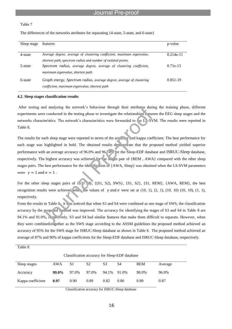
After testing and analysing the network’s behaviour through their attributes during the training phase, different

experiments were conducted in the testing phase to investigate the relationships between the EEG sleep stages and the

networks characteristics. The network’s characteristics were forwarded to the LS-SVM. The results were reported in

Table 8.

The results for each sleep stage were reported in terms of the accuracy and kappa coefficient. The best performance for

each stage was highlighted in bold. The obtained results demonstrate that the proposed method yielded superior

performance with an average accuracy of 96.0% and 96.74% for the Sleep-EDF database and ISRUC-Sleep database,

respectively. The highest accuracy was achieved for the stages pair of {REM , AWA} compared with the other sleep

stages pairs. The best performance for the identification of {AWA, Sleep} was obtained when the LS-SVM parameters

were .

For the other sleep stages pairs of {S3, S4}, {(S1, S2), SWS}, {S1, S2}, {S1, REM}, {AWA, REM}, the best

recognition results were achieved when the values of were set at (10, 1), (2, 1), (10, 10) (10, 10), (1, 1),

respectively.

From the results in Table 8 , it was noticed that when S3 and S4 were combined as one stage of SWS, the classification

accuracy by the proposed method was improved. The accuracy for identifying the stages of S3 and S4 in Table 8 are

94.1% and 91.0%, respectively. S3 and S4 had similar features that make them difficult to separate. However, when

they were combined together as the SWS stage according to the ASSM guidelines the proposed method achieved an

accuracy of 95% for the SWS stage for ISRUC-Sleep database as shown in Table 8. The proposed method achieved an

average of 87% and 90% of kappa coefficients for the Sleep-EDF database and ISRUC-Sleep database, respectively.

Table 8

Classification accuracy for Sleep-EDF database

Sleep stages AWA S1 S2 S3 S4 REM Average

Accuracy 99.0% 97.0% 97.0% 94.1% 91.0% 98.0% 96.0%

Kappa coefficient 0.97 0.90 0.89 0.82 0.80 0.89 0.87

Classification accuracy for ISRUC-Sleep database

Table 7

The differences of the networks attributes for separating {4-state, 5-state, and 6-state}

Sleep stage features p-value

4-state Average degree, average of clustering coefficient, maximum eigenvalue,

shortest path, spectrum radius and number of isolated points.

0.214e-11

5-state Spectrum radius, average degree, average of clustering coefficient,

maximum eigenvalue, shortest path.

0.71e-13

6-state Graph energy, Spectrum radius, average degree, average of clustering

coefficient, maximum eigenvalue, shortest path

0.851-19

17

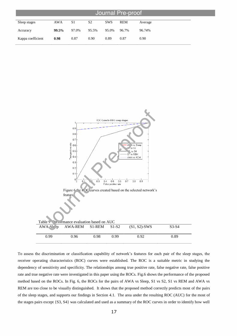
To assess the discrimination or classification capability of network’s features for each pair of the sleep stages, the

receiver operating characteristics (ROC) curves were established. The ROC is a suitable metric in studying the

dependency of sensitivity and specificity. The relationships among true positive rate, false negative rate, false positive

rate and true negative rate were investigated in this paper using the ROCs. Fig.6 shows the performance of the proposed

method based on the ROCs. In Fig. 6, the ROCs for the pairs of AWA vs Sleep, S1 vs S2, S1 vs REM and AWA vs

REM are too close to be visually distinguished. It shows that the proposed method correctly predicts most of the pairs

of the sleep stages, and supports our findings in Section 4.1. The area under the resulting ROC (AUC) for the most of

the stages pairs except {S3, S4} was calculated and used as a summary of the ROC curves in order to identify how well

Sleep stages AWA S1 S2 SWS REM Average

Accuracy 99.5% 97.0% 95.5% 95.0% 96.7% 96.74%

Kappa coefficient 0.98 0.87 0.90 0.89 0.87 0.90

Table 9 Performance evaluation based on AUC

AWA-Sleep

AWA-REM S1-REM S1-S2 (S1, S2)-SWS S3-S4

0.99

0.96 0.98 0.99 0.92 0.89

Figure 6 the ROC curves created based on the selected network’s

feature

18

those networks features could discriminate each pair of EEG sleep stages. The AUC is a portion of the area under the

ROC curves. The AUC values ranges from 0.5 (without discrimination) to 1.0 (ideal discrimination). Table 9 shows the

AUC values obtained from each classification pair. The maximum AUC value was 0.99 for the pair of {AWA, sleep},

while the minimum value was 0.89 for the pair of {S3, S4} due to the sleep stages S3 and S4 often have similar

networks features.

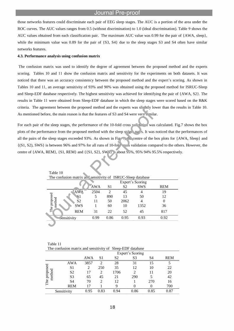
4.3. Performance analysis using confusion matrix

The confusion matrix was used to identify the degree of agreement between the proposed method and the experts

scoring. Tables 10 and 55 show the confusion matrix and sensitivity for the experiments on both datasets. It was

noticed that there was an accuracy consistency between the proposed method and the expert’s scoring. As shown in

Tables 50 and 15, an average sensitivity of 93% and 90% was obtained using the proposed method for ISRUC-Sleep

and Sleep-EDF database respectively. The highest sensitivity was achieved for identifying the pair of {AWA, S2}. The

results in Table 15 were obtained from Sleep-EDF database in which the sleep stages were scored based on the R&K

criteria. The agreement between the proposed method and the experts was slightly lower than the results in Table 10.

As mentioned before, the main reason is that the features of S3 and S4 were very similar.

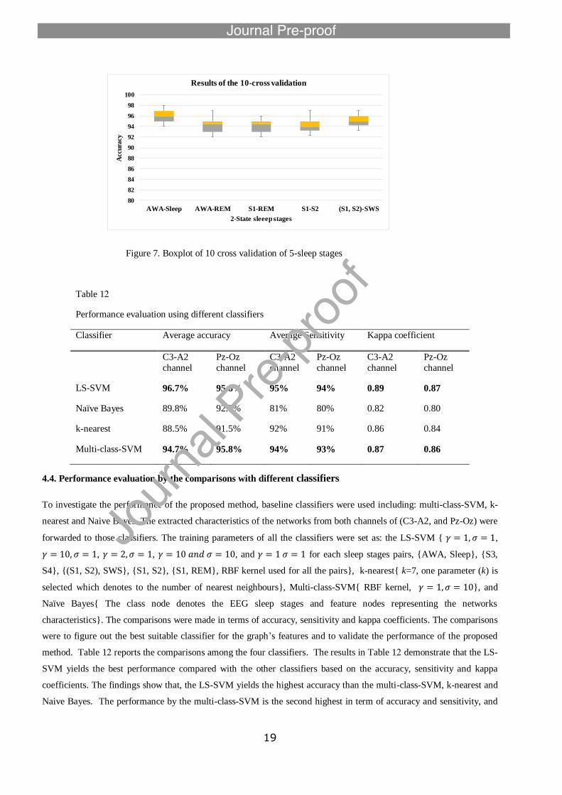
For each pair of the sleep stages, the performance of the 10-fold cross validation was calculated. Fig.7 shows the box

plots of the performance from the proposed method with the sleep stages pairs. It was noticed that the performances of

all the pairs of the sleep stages exceeded 93%. As shown in Fig. 7, the centre of the box plots for {AWA, Sleep} and

{(S1, S2), SWS} is between 96% and 97% for all runs of 10-fold cross validation compared to the others. However, the

centre of {AWA, REM}, {S1, REM} and {{S1, S2}, SWS} is about 95%, 95% 94% 95.5% respectively.

Table 50

The confusion matrix and sensitivity of ISRUC-Sleep database

Expert’s Scoring

AWA S1 S2 SWS REM

The

pro

pose

d

met

hod

AWA 2504 2 45 4 19

S1 5 890 13 50 12

S2 11 50 2062 4 0

SWS 1 60 10 1352 36

REM 31 22 52 45 817

Sensitivity 0.99 0.86 0.95 0.93 0.92

Table 15 The confusion matrix and sensitivity of Sleep-EDF database

Expert’s Scoring

AWA S1 S2 S3 S4 REM

The

pro

pose

d

met

hod

AWA 3857 2 28 31 15 5

S1 2 250 35 12 10 22

S2 17 2 1706 2 11 20

S3 65 45 21 290 5 42

S4 70 2 12 1 270 16

REM 17 1 9 0 0 700

Sensitivity 0.95 0.83 0.94 0.86 0.85 0.87

19

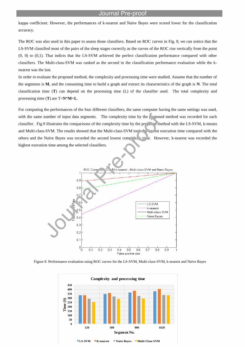
4.4. Performance evaluation by the comparisons with different classifiers

To investigate the performance of the proposed method, baseline classifiers were used including: multi-class-SVM, k-

nearest and Naive Bayes. The extracted characteristics of the networks from both channels of (C3-A2, and Pz-Oz) were

forwarded to those classifiers. The training parameters of all the classifiers were set as: the LS-SVM { ,

, , , and for each sleep stages pairs, {AWA, Sleep}, {S3,

S4}, {(S1, S2), SWS}, {S1, S2}, {S1, REM}, RBF kernel used for all the pairs}, k-nearest{ k=7, one parameter (k) is

selected which denotes to the number of nearest neighbours}, Multi-class-SVM{ RBF kernel, }, and

Naïve Bayes{ The class node denotes the EEG sleep stages and feature nodes representing the networks

characteristics}. The comparisons were made in terms of accuracy, sensitivity and kappa coefficients. The comparisons

were to figure out the best suitable classifier for the graph’s features and to validate the performance of the proposed

method. Table 12 reports the comparisons among the four classifiers. The results in Table 12 demonstrate that the LS-

SVM yields the best performance compared with the other classifiers based on the accuracy, sensitivity and kappa

coefficients. The findings show that, the LS-SVM yields the highest accuracy than the multi-class-SVM, k-nearest and

Naive Bayes. The performance by the multi-class-SVM is the second highest in term of accuracy and sensitivity, and

Table 12

Performance evaluation using different classifiers

Classifier Average accuracy Average Sensitivity Kappa coefficient

C3-A2

channel

Pz-Oz

channel

C3-A2

channel

Pz-Oz

channel

C3-A2

channel

Pz-Oz

channel

LS-SVM 96.7% 95.8% 95% 94% 0.89 0.87

Naïve Bayes 89.8% 92.3% 81% 80% 0.82 0.80

k-nearest 88.5% 91.5% 92% 91% 0.86 0.84

Multi-class-SVM 94.7% 95.8% 94% 93% 0.87 0.86

Figure 7. Boxplot of 10 cross validation of 5-sleep stages

80

82

84

86

88

90

92

94

96

98

100

AWA-Sleep AWA-REM S1-REM S1-S2 (S1, S2)-SWS

Acc

ura

cy

2-State sleeep stages

Results of the 10-cross validation

20

kappa coefficient. However, the performances of k-nearest and Naive Bayes were scored lower for the classification

accuracy.

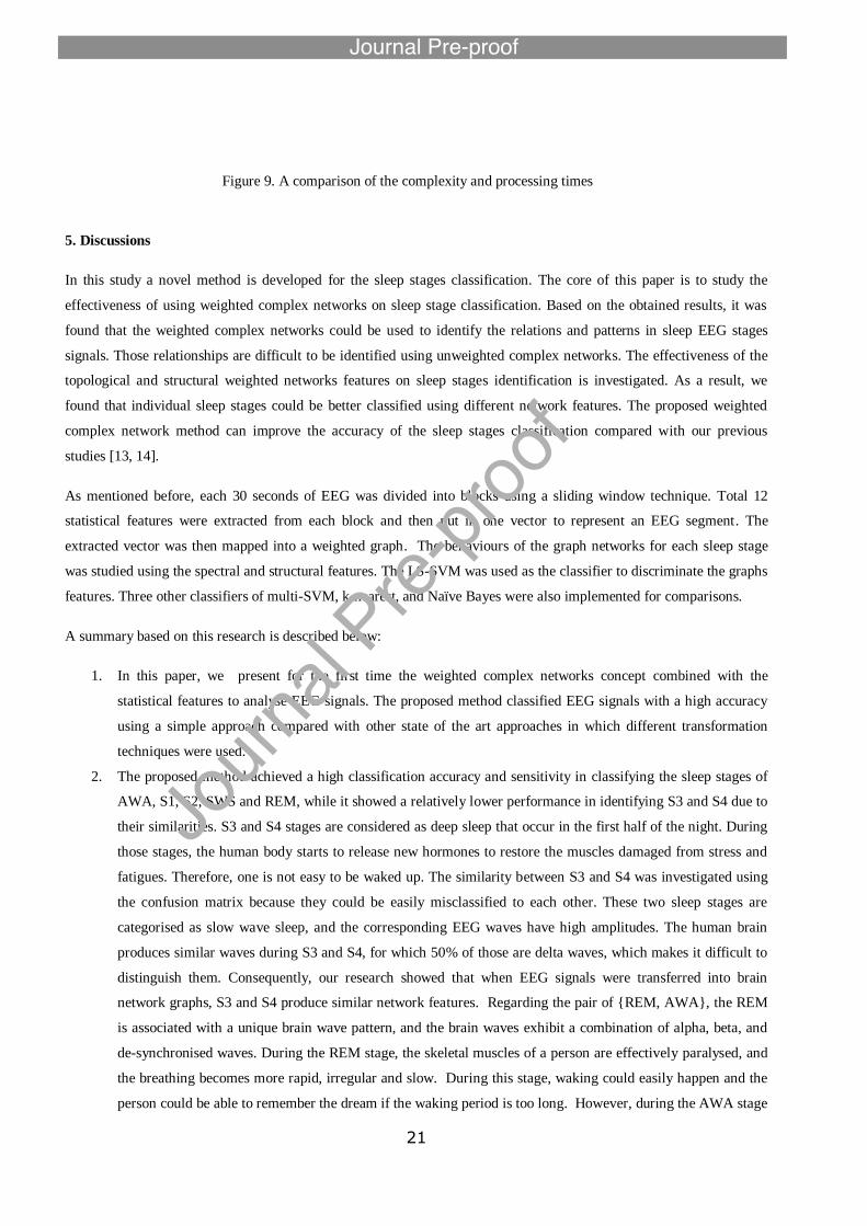
The ROC was also used in this paper to assess those classifiers. Based on ROC curves in Fig. 8, we can notice that the

LS-SVM classified most of the pairs of the sleep stages correctly as the curves of the ROC rise vertically from the point

(0, 0) to (0,1). That indicts that the LS-SVM achieved the perfect classification performance compared with other

classifiers. The Multi-class-SVM was ranked as the second in the classification performance evaluation while the k-

nearest was the last.

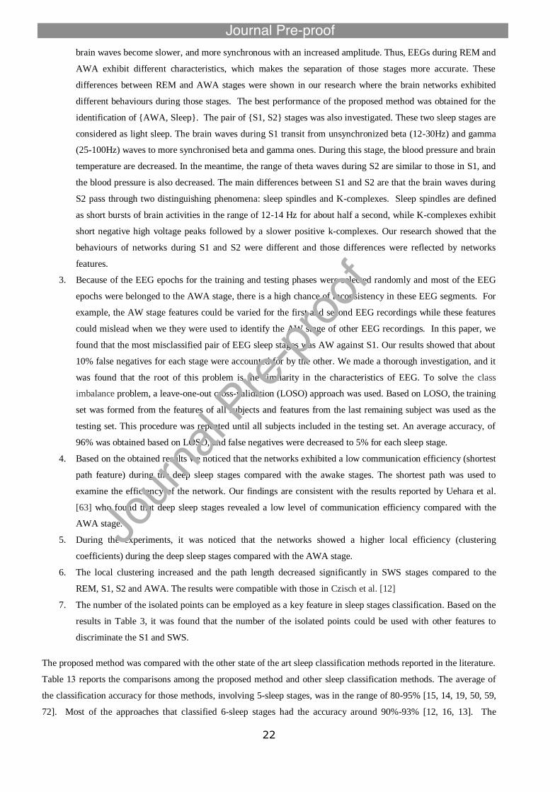
In order to evaluate the proposed method, the complexity and processing time were studied. Assume that the number of

the segments is M, and the consuming time to build a graph and extract its characteristics of the graph is N. The total

classification time (T) can depend on the processing time (L) of the classifier used. The total complexity and

processing time (T) are T=N*M+L.

For computing the performances of the four different classifiers, the same computer having the same settings was used,

with the same number of input data segments. The complexity time by the proposed method was recorded for each

classifier. Fig.9 illustrates the comparisons of the complexity time by the proposed method with the LS-SVM, k-means

and Multi-class-SVM. The results showed that the Multi-class-SVM took the lowest execution time compared with the

others and the Naïve Bayes was recorded the second lowest complexity time. However, k-nearest was recorded the

highest execution time among the selected classifiers.

Figure 8. Performance evaluation using ROC curves for the LS-SVM, Multi-class-SVM, k-nearest and Naïve Bayes

0

50

100

150

200

250

300

350

400

450

120 300 900 1620

Tim

e (

S)

Segment No.

Complexity and processing time

LS-SVM K-nearset Naïve Bayes Multi-Class-SVM

21

5. Discussions

In this study a novel method is developed for the sleep stages classification. The core of this paper is to study the

effectiveness of using weighted complex networks on sleep stage classification. Based on the obtained results, it was

found that the weighted complex networks could be used to identify the relations and patterns in sleep EEG stages

signals. Those relationships are difficult to be identified using unweighted complex networks. The effectiveness of the

topological and structural weighted networks features on sleep stages identification is investigated. As a result, we

found that individual sleep stages could be better classified using different network features. The proposed weighted

complex network method can improve the accuracy of the sleep stages classification compared with our previous

studies [13, 14].

As mentioned before, each 30 seconds of EEG was divided into blocks using a sliding window technique. Total 12

statistical features were extracted from each block and then put in one vector to represent an EEG segment. The

extracted vector was then mapped into a weighted graph. The behaviours of the graph networks for each sleep stage

was studied using the spectral and structural features. The LS-SVM was used as the classifier to discriminate the graphs

features. Three other classifiers of multi-SVM, k-nearest, and Naïve Bayes were also implemented for comparisons.

A summary based on this research is described below:

1. In this paper, we present for the first time the weighted complex networks concept combined with the

statistical features to analyse EEG signals. The proposed method classified EEG signals with a high accuracy

using a simple approach compared with other state of the art approaches in which different transformation

techniques were used.

2. The proposed method achieved a high classification accuracy and sensitivity in classifying the sleep stages of

AWA, S1, S2, SWS and REM, while it showed a relatively lower performance in identifying S3 and S4 due to

their similarities. S3 and S4 stages are considered as deep sleep that occur in the first half of the night. During

those stages, the human body starts to release new hormones to restore the muscles damaged from stress and

fatigues. Therefore, one is not easy to be waked up. The similarity between S3 and S4 was investigated using

the confusion matrix because they could be easily misclassified to each other. These two sleep stages are

categorised as slow wave sleep, and the corresponding EEG waves have high amplitudes. The human brain

produces similar waves during S3 and S4, for which 50% of those are delta waves, which makes it difficult to

distinguish them. Consequently, our research showed that when EEG signals were transferred into brain

network graphs, S3 and S4 produce similar network features. Regarding the pair of {REM, AWA}, the REM

is associated with a unique brain wave pattern, and the brain waves exhibit a combination of alpha, beta, and

de-synchronised waves. During the REM stage, the skeletal muscles of a person are effectively paralysed, and

the breathing becomes more rapid, irregular and slow. During this stage, waking could easily happen and the

person could be able to remember the dream if the waking period is too long. However, during the AWA stage

Figure 9. A comparison of the complexity and processing times

22

brain waves become slower, and more synchronous with an increased amplitude. Thus, EEGs during REM and

AWA exhibit different characteristics, which makes the separation of those stages more accurate. These

differences between REM and AWA stages were shown in our research where the brain networks exhibited

different behaviours during those stages. The best performance of the proposed method was obtained for the

identification of {AWA, Sleep}. The pair of {S1, S2} stages was also investigated. These two sleep stages are

considered as light sleep. The brain waves during S1 transit from unsynchronized beta (12-30Hz) and gamma

(25-100Hz) waves to more synchronised beta and gamma ones. During this stage, the blood pressure and brain

temperature are decreased. In the meantime, the range of theta waves during S2 are similar to those in S1, and

the blood pressure is also decreased. The main differences between S1 and S2 are that the brain waves during

S2 pass through two distinguishing phenomena: sleep spindles and K-complexes. Sleep spindles are defined

as short bursts of brain activities in the range of 12-14 Hz for about half a second, while K-complexes exhibit

short negative high voltage peaks followed by a slower positive k-complexes. Our research showed that the

behaviours of networks during S1 and S2 were different and those differences were reflected by networks

features.

3. Because of the EEG epochs for the training and testing phases were selected randomly and most of the EEG

epochs were belonged to the AWA stage, there is a high chance of inconsistency in these EEG segments. For

example, the AW stage features could be varied for the first and second EEG recordings while these features

could mislead when we they were used to identify the AW stage of other EEG recordings. In this paper, we

found that the most misclassified pair of EEG sleep stages was AW against S1. Our results showed that about

10% false negatives for each stage were accounted for by the other. We made a thorough investigation, and it

was found that the root of this problem is the similarity in the characteristics of EEG. To solve the class

imbalance problem, a leave-one-out cross-validation (LOSO) approach was used. Based on LOSO, the training

set was formed from the features of all subjects and features from the last remaining subject was used as the

testing set. This procedure was repeated until all subjects included in the testing set. An average accuracy, of

96% was obtained based on LOSO, and false negatives were decreased to 5% for each sleep stage.

4. Based on the obtained results we noticed that the networks exhibited a low communication efficiency (shortest

path feature) during the deep sleep stages compared with the awake stages. The shortest path was used to

examine the efficiency of the network. Our findings are consistent with the results reported by Uehara et al.

[63] who found that deep sleep stages revealed a low level of communication efficiency compared with the

AWA stage.

5. During the experiments, it was noticed that the networks showed a higher local efficiency (clustering

coefficients) during the deep sleep stages compared with the AWA stage.

6. The local clustering increased and the path length decreased significantly in SWS stages compared to the

REM, S1, S2 and AWA. The results were compatible with those in Czisch et al. [12]

7. The number of the isolated points can be employed as a key feature in sleep stages classification. Based on the

results in Table 3, it was found that the number of the isolated points could be used with other features to

discriminate the S1 and SWS.

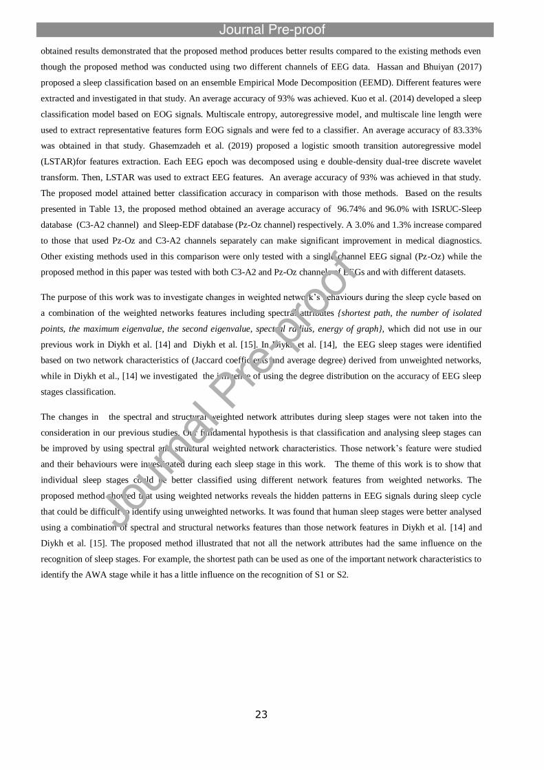
The proposed method was compared with the other state of the art sleep classification methods reported in the literature.

Table 13 reports the comparisons among the proposed method and other sleep classification methods. The average of

the classification accuracy for those methods, involving 5-sleep stages, was in the range of 80-95% [15, 14, 19, 50, 59,

72]. Most of the approaches that classified 6-sleep stages had the accuracy around 90%-93% [12, 16, 13]. The

23

obtained results demonstrated that the proposed method produces better results compared to the existing methods even

though the proposed method was conducted using two different channels of EEG data. Hassan and Bhuiyan (2017)

proposed a sleep classification based on an ensemble Empirical Mode Decomposition (EEMD). Different features were

extracted and investigated in that study. An average accuracy of 93% was achieved. Kuo et al. (2014) developed a sleep

classification model based on EOG signals. Multiscale entropy, autoregressive model, and multiscale line length were

used to extract representative features form EOG signals and were fed to a classifier. An average accuracy of 83.33%

was obtained in that study. Ghasemzadeh et al. (2019) proposed a logistic smooth transition autoregressive model

(LSTAR)for features extraction. Each EEG epoch was decomposed using e double-density dual-tree discrete wavelet

transform. Then, LSTAR was used to extract EEG features. An average accuracy of 93% was achieved in that study.

The proposed model attained better classification accuracy in comparison with those methods. Based on the results

presented in Table 13, the proposed method obtained an average accuracy of 96.74% and 96.0% with ISRUC-Sleep

database (C3-A2 channel) and Sleep-EDF database (Pz-Oz channel) respectively. A 3.0% and 1.3% increase compared

to those that used Pz-Oz and C3-A2 channels separately can make significant improvement in medical diagnostics.

Other existing methods used in this comparison were only tested with a single channel EEG signal (Pz-Oz) while the

proposed method in this paper was tested with both C3-A2 and Pz-Oz channels of EEGs and with different datasets.

The purpose of this work was to investigate changes in weighted network’s behaviours during the sleep cycle based on

a combination of the weighted networks features including spectral attributes {shortest path, the number of isolated

points, the maximum eigenvalue, the second eigenvalue, spectral radius, energy of graph}, which did not use in our

previous work in Diykh et al. [14] and Diykh et al. [15]. In Diykh et al. [14], the EEG sleep stages were identified

based on two network characteristics of (Jaccard coefficients and average degree) derived from unweighted networks,

while in Diykh et al., [14] we investigated the influence of using the degree distribution on the accuracy of EEG sleep

stages classification.

The changes in the spectral and structural weighted network attributes during sleep stages were not taken into the

consideration in our previous studies. Our fundamental hypothesis is that classification and analysing sleep stages can

be improved by using spectral and structural weighted network characteristics. Those network’s feature were studied

and their behaviours were investigated during each sleep stage in this work. The theme of this work is to show that

individual sleep stages could be better classified using different network features from weighted networks. The

proposed method showed that using weighted networks reveals the hidden patterns in EEG signals during sleep cycle

that could be difficult to identify using unweighted networks. It was found that human sleep stages were better analysed

using a combination of spectral and structural networks features than those network features in Diykh et al. [14] and

Diykh et al. [15]. The proposed method illustrated that not all the network attributes had the same influence on the

recognition of sleep stages. For example, the shortest path can be used as one of the important network characteristics to

identify the AWA stage while it has a little influence on the recognition of S1 or S2.

24

Table 53

The accuracy comparison with the existing methods in the literature

Authors Sleep stages EEG channel

Method and main characteristics Number or type of features Accuracy

Zhu et al. [72]

AWA, S1,

S2, S3, S4 and REM

Pz-Oz

The differences of mean degrees

between horizontal and

vertical visibility graphs were used to classify sleep EEG signals

Seven features extracted

from Visibility graphs

87%

Peker et al. [50] AWA, S1,

S2, SWS, REM

C3-A2 Combining a duel tree complex

wavelet (DTCWT) and a complex-

valued neural network

The statistical features of

DTCWT coefficients

95.42%,

93.84 with

AASM and

R&K criteria

respectively

Da Silveira et al. [13] AWA, S1,

S2, S3, S4 and REM

PZ-OZ A normalized wavelet transform and

a random forest classifier

The statistical features of the

discrete wavelet transform

91%

Shi et al. [58] AWA, S1,

S2, S3, S4

and REM

C3-A2,

C3-A1

A join collaborative representation model

Seven features extracted

from visibility graphs

80.29%

Sinha et al. [59] AWA, REM

and sleep

spindles

N/A Combined Discrete wavelet (DW) with neural networks

DW coefficients 95.35%

Ebrahimi et al. [17] AWA, S1,

S2, SWS and REM

Pz-Oz, Fpz-Cz

Wavelet package coefficients combined with a neural network.

Five statistical features were

extracted from Wavelet

package coefficients

93.0±4.0%

Fraiwan et al. [18] AWA, S1,

S2, S3, S4 and REM

C3-A2,

Fpz-Cz

Continuous wavelet transform and a

linear discrimination analysis.

Time Frequency Entropy

features

84%

Hsu et al. [24] AWA, S1,

S2, SWS and REM

Pz-Oz, Fpz-Cz

Energy features of EEG signals with an Elman recurrent neural network

Six energy feature extracted

from six characteristic waves

of EEGs

90.93%

Hassan and Bhuiyan

[23]

AWA, S1,

S2, S3, S4 and REM

C3-A2 ensemble Empirical Mode

Decomposition

Statistical features 93%

Kuo et al. [ 33] AWA, S1,

S2, SWS and

REM

EOG signals Butterworth band-pass filter MSE, AR, and MLL

83.33%

Ghasemzadeh et al. [20] AWA, S1,

S2, S3, S4 and REM

C3-A2, Pz-oz

D3TDWT based on LSTAR LSTAR coefficients 93%

Diykh et al. [14] AWA, S1,

S2, S3, S4 and REM

C3-A2 Structural graph features combined

with k-means

Three networks features 95.93%

Diykh et al. [15] S1, S2, S3, S4 and REM

Undirected complex networks combined with statistical features

Four networks features 92.16

The proposed method AWA, S1,

S2, S3, S4 and REM

Pz-Oz Weighted networks and LS-SVM 8 network features 96.0%

The proposed method AWA, S1,

S2, SWS and

REM

C3-A2 Weighted networks and LS-SVM 8 network features 96.74%

25

6. Conclusion

In this paper, the characteristics of complex networks which were constructed from 12 statistical features of EEG

signals were extracted to identify the sleep stages. The study examined the efficiency of the topological and structural

attributes of the weighted undirected networks in the sleep stages classification. Different networks attributes were used

and tested. One of the most important findings in this paper was that the behaviours of networks could vary from one

sleep stage to the others. The effectiveness of the proposed method was tested with two datasets that were acquired

from different EEG channels. The proposed method achieved a high classification accuracy according to the AASM

compared with the R&K guidelines.

In this work, the obtained results showed that using imbalance EEG data had negative effects on classification accuracy

and the performance of the proposed method. Our future work will focus on testing different approaches such as

oversample the minority, under-sample the majority classes, and synthesize them both to tackle this issue. In addition,

more balanced EEG dataset will be employed to evaluate the proposed method. Big data technologies will also be

applied to further improve the algorithm. The proposed method can contribute to develop a system tool for automatic

sleep stages scoring which can be useful to assist doctors and neurologists for the diagnostics and treatment of sleep

disorders and for sleep research.

Conflict of interest

Authors declare that there is no conflict of interest in this paper.

Acknowledgment

Authors would like to thank University of Southern Queensland for its support. We also thank all reviewers and the

journal Editor-in-Chief for considering this paper and facilitating the review process.

References

[1] S. Abdulla, M. Diykh, R.L. Lafta, K. Saleh, and R.C. Deo, Sleep EEG signal analysis based on correlation graph

similarity coupled with an ensemble extreme machine learning algorithm, Expert Systems with Applications, 138

(2019) 1-15.

[2] U.R. Acharya, E.C.-P. Chua, K.C. Chua, L.C. Min, T. Tamura, Analysis and automatic identification of sleep stages

using higher order spectra, International journal of neural systems, 20 (2010) 509-521.

[3] U.R. Acharya, S.V. Sree, G. Swapna, R.J. Martis, J.S. Suri, Automated EEG analysis of epilepsy: a review,

Knowledge-Based Systems, 45 (2013) 147-165.

[4] H.R. Al Ghayab, Y. Li, S. Abdulla, M. Diykh, X. Wan, Classification of epileptic EEG signals based on simple

random sampling and sequential feature selection, Brain Informatics, 3 (2016) 85-91.

[5] H.U. Amin, A.S. Malik, N. Kamel, M. Hussain, A Novel Approach Based on Data Redundancy for Feature

Extraction of EEG Signals, Brain topography, 29 (2016) 207-217.

[6] S. Aydın, M.A. Tunga, S. Yetkin, Mutual information analysis of sleep eeg in detecting psycho-physiological

insomnia, Journal of medical systems, 39 (2015) 1-10.

[7] V. Bajaj, R.B. Pachori, Automatic classification of sleep stages based on the time-frequency image of EEG signals,

Computer Methods and Programs in Biomedicine, 112 (2013) 320-328.

26

[8] Y. Bennani, K. Benabdeslem, Dendogram-based SVM for multi-class classification, CIT. Journal of computing and

information technology, 14 (2006) 283-289.

[9] R.B. Berry, R. Brooks, C.E. Gamaldo, S.M. Harding, C. Marcus, B. Vaughn, The AASM manual for the scoring of

sleep and associated events, Rules, Terminology and Technical Specifications, Darien, Illinois, American Academy of

Sleep Medicine, (2012).

[10] L.-l. Chen, Y. Zhao, J. Zhang, J.-z. Zou, Automatic detection of alertness/drowsiness from physiological signals

using wavelet-based nonlinear features and machine learning, Expert Systems with Applications, 42 (2015) 7344-7355.

[11] D.M. Cvetković, M. Doob, H. Sachs, Spectra of graphs: theory and application, Academic Pr, 1980.

[12] M. Czisch, V.I. Spoormaker, K.C. Andrade, R. Wehrle, P.G. Sämannn, User Research Sleep and functional

imaging, Brain, 41 (2011) 5-8.

[13] T.L. da Silveira, A.J. Kozakevicius, C.R. Rodrigues, Single-channel EEG sleep stage classification based on a

streamlined set of statistical features in wavelet domain, Medical & biological engineering & computing, (2016) 1-10.

[14] M. Diykh, Y. Li, Complex networks approach for EEG signal sleep stages classification, Expert Systems with

Applications, 63 (2016) 241-248.

[15] M. Diykh, Y. Li, P. Wen, EEG Sleep Stages Classification Based on Time Domain Features and Structural Graph

Similarity, IEEE Transactions on Neural Systems and Rehabilitation Engineering, 24. (2016): 1159-1168.

[16] M. Diykh, Y. Li, P. Wen, T. Li, Complex networks approach for depth of anesthesia assessment, Measurement,

119 (2018) 178-189.

[17] F. Ebrahimi, M. Mikaeili, E. Estrada, H. Nazeran, Automatic sleep stage classification based on EEG signals by

using neural networks and wavelet packet coefficients, in: 2008 30th Annual International Conference of the IEEE

Engineering in Medicine and Biology Society, IEEE, 2008, pp. 1151-1154.

[18] L. Fraiwan, K. Lweesy, N. Khasawneh, M. Fraiwan, H. Wenz, H. Dickhaus, Classification of sleep stages using

multi-wavelet time frequency entropy and LDA, Methods of information in Medicine, 49 (2010) 230.

[19] V. Gao, F. Turek, M. Vitaterna, Multiple classifier systems for automatic sleep scoring in mice, Journal of

neuroscience methods, 264 (2016) 33-39.

[20] P. Ghasemzadeh, H. Kalbkhani, S. Sartipi, M.G. Shayesteh, Classification of sleep stages based on LSTAR model,

Applied Soft Computing, 75 (2019) 523-536.

[21] E.P. Giri, A.M. Arymurthy, M.I. Fanany, S.K. Wijaya, Sleep stages classification using shallow classifiers, in:

2015 International Conference on Advanced Computer Science and Information Systems (ICACSIS), IEEE, 2015, pp.

297-301.

[22] A.L. Goldberger, L.A. Amaral, L. Glass, J.M. Hausdorff, P.C. Ivanov, R.G. Mark, J.E. Mietus, G.B. Moody, C.-K.

Peng, H.E. Stanley, PhysioBank, PhysioToolkit, and PhysioNet: components of a new research resource for complex

physiologic signals, Circulation, 101 (2000) e215-e220.

[23] A.R. Hassan, M.I.H. Bhuiyan, Automated identification of sleep states from EEG signals by means of ensemble

empirical mode decomposition and random under sampling boosting, Computer Methods and Programs in Piomedicine,

140 (2017) 201-210.

[24] Y.-L. Hsu, Y.-T. Yang, J.-S. Wang, C.-Y. Hsu, Automatic sleep stage recurrent neural classifier using energy

features of EEG signals, Neurocomputing, 104 (2013) 105-114.

[25] D. JIANG, M. Yu, W. Yuanyuan, Sleep stage classification using covariance features of multi-channel

physiological signals on Riemannian manifolds, Computer Methods and Programs in Biomedicine, (2019).

27

[26] D. Jiang, Y.-n. Lu, M. Yu, W. Yuanyuan, Robust sleep stage classification with single-channel EEG signals using

multimodal decomposition and HMM-based refinement, Expert Systems with Applications, 121 (2019) 188-203.

[27] G.H. John, P. Langley, Estimating continuous distributions in Bayesian classifiers, in: Proceedings of the Eleventh

conference on Uncertainty in artificial intelligence, Morgan Kaufmann Publishers Inc., 1995, pp. 338-345.

[28] T. Kayikcioglu, M. Maleki, K. Eroglu, Fast and accurate PLS-based classification of EEG sleep using single

channel data, Expert Systems with Applications, 42 (2015) 7825-7830.

[29] B. Kemp, A. Värri, A.C. Rosa, K.D. Nielsen, J. Gade, A simple format for exchange of digitized polygraphic

recordings, Electroencephalography and clinical neurophysiology, 82 (1992) 391-393.

[30] B. Kemp, A.H. Zwinderman, B. Tuk, H.A. Kamphuisen, J.J. Oberye, Analysis of a sleep-dependent neuronal

feedback loop: the slow-wave microcontinuity of the EEG, IEEE Transactions on Biomedical Engineering, 47 (2000)

1185-1194.

[31] S. Khalighi, T. Sousa, G. Pires, U. Nunes, Automatic sleep staging: a computer assisted approach for optimal

combination of features and polysomnographic channels, Expert Systems with Applications, 40 (2013) 7046-7059.

[32] S. Khalighi, T. Sousa, J.M. Santos, U. Nunes, ISRUC-Sleep: A comprehensive public dataset for sleep researchers,

Computer Methods and Programs in Biomedicine, 124 (2016) 180-192.

[33] C.-E. Kuo, S.-F. Liang, Y.-C. Li, F.-Y. Cherng, W.-C. Lin, P.-Y. Chen, Y.-C. Liu, F.-Z. Shaw, An EOG-based

Sleep Monitoring System and Its Application on On-line Sleep-stage Sensitive Light Control, PhyCS, 2014, pp. 20-30.

[34] T. Lajnef, S. Chaibi, P. Ruby, P.-E. Aguera, J.-B. Eichenlaub, M. Samet, A. Kachouri, K. Jerbi, Learning

machines and sleeping brains: automatic sleep stage classification using decision-tree multi-class support vector

machines, Journal of neuroscience methods, 250 (2015) 94-105.

[35] J.-M. Lee, D.-J. Kim, I.-Y. Kim, K.S. Park, S.I. Kim, Nonlinear-analysis of human sleep EEG using detrended

fluctuation analysis, Medical engineering & physics, 26 (2004) 773-776.

[36] G. Li, M. Semerci, B. Yener, M.J. Zaki, Graph classification via topological and label attributes, in: Proceedings

of the 9th international workshop on mining and learning with graphs (MLG), San Diego, USA, 2011.

[37] G. Li, M. Semerci, B. Yener, M.J. Zaki, Effective graph classification based on topological and label attributes,

Statistical Analysis and Data Mining, 5 (2012) 265-283.

[38] T. Li, P. Wen, Depth of anaesthesia assessment based on adult electroencephalograph beta frequency band,

Australasian Physical & Engineering Sciences in Medicine, 39 (2016) 773-781.

[39] T. Li, P. Wen, Depth of anaesthesia assessment using interval second-order difference plot and permutation

entropy techniques, IET Signal Processing, 11 (2016) 221-227.

[40] [34] Siuly, Y. Li, P.P. Wen, Clustering technique-based least square support vector machine for EEG signal

classification, Computer Methods and Programs in bBiomedicine, 104 (2011) 358-372.

[41] S.-F. Liang, C.-E. Kuo, Y.-H. Hu, Y.-H. Pan, Y.-H. Wang, Automatic stage scoring of single-channel sleep EEG

by using multiscale entropy and autoregressive models, IEEE Transactions on Instrumentation and Measurement, 61

(2012) 1649-1657.

[42] Z. Liu, J. Sun, Y. Zhang, P. Rolfe, Sleep staging from the EEG signal using multi-domain feature extraction,

Biomedical Signal Processing and Control, 30 (2016) 86-97.

[43] R.M. Mehmood, H.J. Lee, Exploration of prominent frequency wave in EEG signals from brain sensors network,

International Journal of Distributed Sensor Networks, 11 (2015) 386057.

28

[44] S. Micheloyannis, E. Pachou, C.J. Stam, M. Vourkas, S. Erimaki, V. Tsirka, Using graph theoretical analysis of

multi channel EEG to evaluate the neural efficiency hypothesis, Neuroscience letters, 402 (2006) 273-277.

[45] J. Milgram, M. Cheriet, R. Sabourin, “One Against One” or “One Against All”: Which One is Better for

Handwriting Recognition with SVMs?, in: Tenth International Workshop on Frontiers in Handwriting Recognition,

Suvisoft, La Baule (France), 2006.

[46] M. Mourtazaev, B. Kemp, A. Zwinderman, H. Kamphuisen, Age and gender affect different characteristics of slow

waves in the sleep EEG, SLEEP-NEW YORK-, 18 (1995) 557-557.

[47] Z. Mousavi, T.Y. Rezaii, S. Sheykhivand, A. Farzamnia, S. Razavi, Deep convolutional neural network for

classification of sleep stages from single-channel EEG signals, Journal of neuroscience methods, (2019) 108312.

[48] W. Mumtaz, P.L. Vuong, L. Xia, A.S. Malik, R.B.A. Rashid, Automatic diagnosis of alcohol use disorder using

EEG features, Knowledge-Based Systems, 105 (2016) 48-59.

[49] M. Peker, An efficient sleep scoring system based on EEG signal using complex-valued machine learning

algorithms, Neurocomputing, 207 (2016) 165-177.

[50] M. Peker, A new approach for automatic sleep scoring: Combining Taguchi based complex-valued neural network

and complex wavelet transform, Computer Methods and Programs in Biomedicine, 129 (2016) 203-216.

[51] H. Qiu, E.R. Hancock, Graph matching and clustering using spectral partitions, Pattern Recognition, 39 (2006) 22-

34.

[52] M.M. Rahman, M.I.H. Bhuiyan, A.R. Hassan, Sleep stage classification using single-channel EOG, Computers in

Biology and Medicine, 102 (2018) 211-220.

[53] A. Rechtschaffen, A. Kales, A manual of standardized terminology, techniques and scoring system for sleep stages

of human subjects, (1968).

[54] J.L. Rodríguez-Sotelo, A. Osorio-Forero, A. Jiménez-Rodríguez, D. Cuesta-Frau, E. Cirugeda-Roldán, D. Peluffo,

Automatic sleep stages classification using EEG entropy features and unsupervised pattern analysis techniques,

Entropy, 16 (2014) 6573-6589.

[55] K. Samiee, P. Kovács, M. Gabbouj, Epileptic seizure detection in long-term EEG records using sparse rational

decomposition and local Gabor binary patterns feature extraction, Knowledge-Based Systems, 118 (2017) 228-240.

[56] [49] M. Schmidt, G. Palm, F. Schwenker, Spectral graph features for the classification of graphs and graph

sequences, Computational Statistics, 29 (2014) 65-80.

[57] M. Sharma, A. Dhere, R.B. Pachori, U.R. Acharya, An Automatic Detection of Focal EEG Signals Using New

Class of Time–Frequency Localized Orthogonal Wavelet Filter Banks, Knowledge-Based Systems, 118 (2016) 217-

227.

[58] J. Shi, X. Liu, Y. Li, Q. Zhang, Y. Li, S. Ying, Multi-channel EEG-based sleep stage classification with joint

collaborative representation and multiple kernel learning, Journal of Neuroscience Methods, 254 (2015) 94-101.

[59] R.K. Sinha, Artificial neural network and wavelet based automated detection of sleep spindles, REM sleep and

wake states, Journal of Medical Systems, 32 (2008) 291-299.

[60] T. Sousa, A. Cruz, . Khalighi, G. Pires, U. Nunes, A two-step automatic sleep stage classification method with

dubious range detection, Computers in Biology and Medicine, 59 (2015) 42-53.

[61] J. Suykens, L. Lukas, P. Van Dooren, B. De Moor, J. Vandewalle, Least squares support vector machine

classifiers: a large scale algorithm, in: European Conference on Circuit Theory and Design, ECCTD, Citeseer, 1999,

pp. 839-842.

29

[62] J.A. Suykens, J. Vandewalle, Least squares support vector machine classifiers, Neural Processing Letters, 9 (1999)

293-300.

[63] T. Uehara, T. Yamasaki, T. Okamoto, T. Koike, S. Kan, S. Miyauchi, J.-i. Kira, S. Tobimatsu, Efficiency of a

“small-world” brain network depends on consciousness level: a resting-state fMRI study, Cerebral cortex, 24 (2014)

1529-1539.

[64] B. Van Sweden, B. Kemp, H. Kamphuisen, A. Ver der Velde, Alternative electrode placement in (automatic) sleep

scoring, Sleep, 13 (1990) 279-283.

[66] D.R. Wilson, T.R. Martinez, Reduction techniques for instance-based learning algorithms, Machine Learning, 38

(2000) 257-286.

[67]B. Xia, Q. Li, J. Jia, J. Wang, U. Chaudhary, A. Ramos-Murguialday, N. Birbaumer, Electrooculogram based sleep

stage classification using deep belief network, in: 2015 International Joint Conference on Neural Networks (IJCNN),

IEEE, 2015, pp. 1-5.

[68] J. Zhang, M. Small, Complex network from pseudoperiodic time series: Topology versus dynamics, Physical

review letters, 96 (2006) 238701.

[69]J. Zhang, Y. Wu, J. Bai, F. Chen, Automatic sleep stage classification based on sparse deep belief net and

combination of multiple classifiers, Transactions of the Institute of Measurement and Control, 4 (2015) 435-451,

0142331215587568.

[70] J. Zhou, X.-m. Wu, W.-j. Zeng, Automatic detection of sleep apnea based on EEG detrended fluctuation analysis

and support vector machine, Journal of COMPUTER Clinical Monitoring and Computing, 29 (2015) 767-772.

[71] Y. Zhou, H. Cheng, J.X. Yu, Graph clustering based on structural/attribute similarities, Proceedings of the VLDB

Endowment, 2 (2009) 718-729.

[72] G. Zhu, Y. Li, P.P. Wen, Analysis and classification of sleep stages based on difference visibility graphs from a

single-channel EEG signal, IEEE journal of biomedical and health informatics, 18 (2014) 1813-1821.

[73] G. Zhu, Y. Li, P.P. Wen, S. Wang, Classifying epileptic EEG signals with delay permutation entropy and multi-

scale K-means, in: Signal and Image Analysis for Biomedical and Life Sciences, Springer, 2015, pp. 143-157.

[74] G. Zhu, Y. Li, P.P. Wen, S. Wang, M. Xi, C. Sun, T. Bednarz, T.D. Pham, P. Vallotton, D. Wang, Epileptogenic

focus detection in intracranial EEG based on delay permutation entropy, in: AIP conference proceedings, AIP, 2013,

pp. 31-36.