Eee Handout 2 Matlab

8/8/2019 Eee Handout 2 Matlab

http://slidepdf.com/reader/full/eee-handout-2-matlab 1/23

1

Student’s Handout

Introduction to MATLABWhat is MATLAB:MATLAB stands for MATrix LABoratory .MATLAB is a software package for computation in

engineering, science, and applied mathematics. It offers a powerful programming language, excellent

graphics, and a wide range of expert knowledge. MATLAB is published by and a trademark of The

MathWorks, Inc.

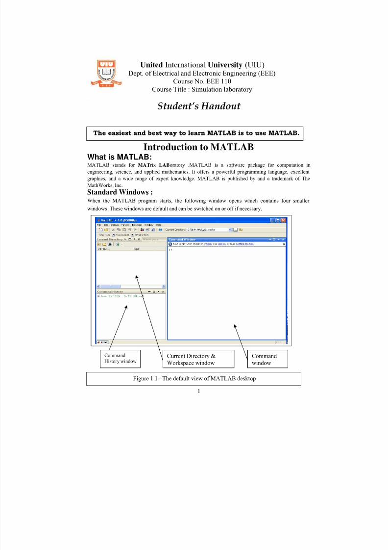
Standard Windows :When the MATLAB program starts, the following window opens which contains four smaller

windows .These windows are default and can be switched on or off if necessary.

United International University (UIU)

Dept. of Electrical and Electronic Engineering (EEE)Course No. EEE 110

Course Title : Simulation laboratory

Command

window

Command

History windowCurrent Directory &

Workspace window

Figure 1.1 : The default view of MATLAB desktop

The easiest and best way to learn MATLAB is to use MATLAB.



2

Four most used MATLAB Windows

Command

Window

This is where you type and execute commands

Workspace

Window

This shows current variables and allows to edit variables by opening array editor (double

click), to load variables from files and to clear variables.

Current

Directory

window

This shows current directory and MATLAB files in current folder, provides with a handy

way to change folders and to load files.

History window This shows previously executed commands. Commands can be re-executed by double-

clicking.

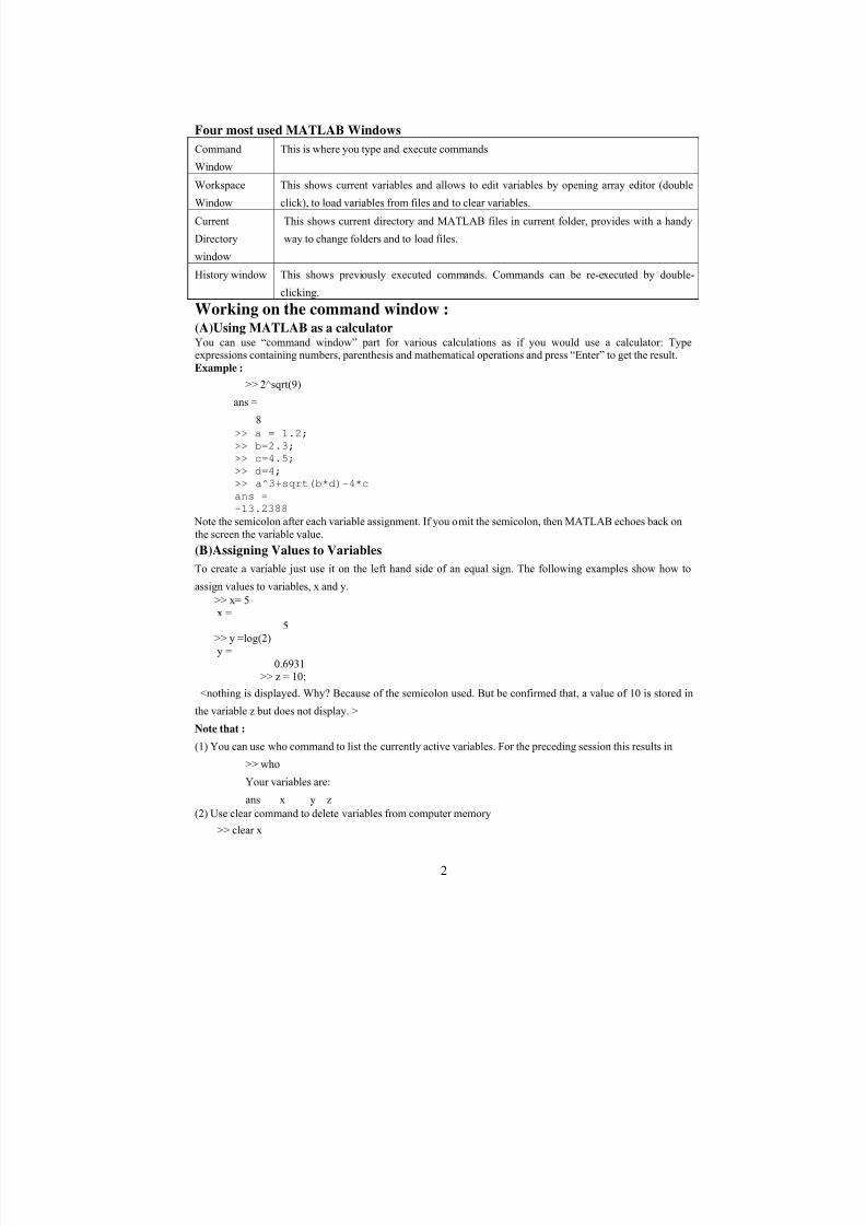
Working on the command window :(A)Using MATLAB as a calculatorYou can use “command window” part for various calculations as if you would use a calculator: Typeexpressions containing numbers, parenthesis and mathematical operations and press “Enter” to get the result.

Example :

>> 2^sqrt(9)

ans =

8

>> a = 1.2;

>> b=2.3;

>> c=4.5;

>> d=4;

>> a^3+sqrt(b*d)-4*c

ans =

-13.2388 Note the semicolon after each variable assignment. If you omit the semicolon, then MATLAB echoes back on

the screen the variable value.

(B)Assigning Values to Variables

To create a variable just use it on the left hand side of an equal sign. The following examples show how to

assign values to variables, x and y.

>> x= 5x =

5>> y =log(2)

y =

0.6931

>> z = 10;<nothing is displayed. Why? Because of the semicolon used. But be confirmed that, a value of 10 is stored in

the variable z but does not display. >

Note that :

(1) You can use who command to list the currently active variables. For the preceding session this results in

>> who

Your variables are:

ans x y z

(2) Use clear command to delete variables from computer memory

>> clear x



3

>> x

??? Undefined function or variable 'x'.

(3) Suppress intermediate output with Semicolon.

MATLAB will print the result of every assignment operation unless the expression on the right hand side is

terminated with a semicolon.

(C)List of useful commands for managing variables :

Command Outcome

clear Removes all variables from memory.

clear x y z Removes only variables x,y,z from the memory .

who Displays a list the variables currently in the memory.

whos Displays a list the variables currently in the memory and their size together with

information about their bytes and class.

(D)Two important command to ensure fairness and readability

Command Outcome

clc Clears contents on the command window ensuring blank working environment

% If used before any line or statement, program ignores the line or statement.

So used to insert any comment in the program.

(E)Predefined variables :

A number of frequently used variables are already defined when MATLAB is started. Some

of the predefined variables are :

Predefined

Variables

Meaning

ans A variable that has the value of the last expression that has not assigned to a specific

variable. If the user does not assign the value of an expression to a variable, MATLAB

automatically stores the result in ans .

pi Value of the number π .

eps The smallest difference between two numbers. It’s value is 2.2204e-016 .

inf Used for infinity.

i or j Defined as 1−

NaN Stands for Not-a-Number.Used when MATLAB cannot determine a valid numeric

value.For example 0/0.

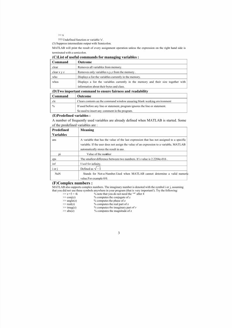
(F)Complex numbers :MATLAB also supports complex numbers. The imaginary number is denoted with the symbol i or j, assuming

that you did not use these symbols anywhere in your program (that is very important!). Try the following:>> z =3 + 4i % note that you do not need the ‘*’ after 4

>> conj(z) % computes the conjugate of z

>> angle(z) % computes the phase of z

>> real(z) % computes the real part of z>> imag(z) % computes the imaginary part of z

>> abs(z) % computes the magnitude of z



4

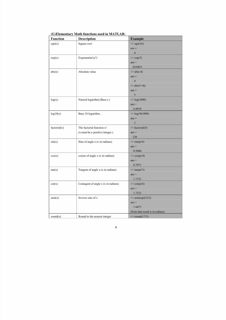
(G)Elementary Math functions used in MATLAB:

Function Description Example

sqrt(x) Square root >> sqrt(16)ans =

4

exp(x) Exponential (ex) >> exp(3)

ans =

20.0855

abs(x) Absolute value >> abs(-4)

ans =

4

>> abs(3+4j)

ans =

5

log(x) Natural logarithm (Base e ) >> log(1000)

ans =

6.9078

log10(x) Base 10 logarithm . >> log10(1000)

ans =

3

factorial(x) The factorial function x!

(x must be a positive integer.)

>> factorial(5)

ans =

120

sin(x) Sine of angle x (x in radians) >> sin(pi/6)

ans =

0.5000

cos(x) cosine of angle x (x in radians) >> cos(pi/4)

ans =

0.7071

tan(x) Tangent of angle x (x in radians) >> tan(pi/3)

ans =

1.7321

cot(x) Cotangent of angle x (x in radians) >> cot(pi/6)

ans =

1.7321

asin(x) Inverse sine of x >> asin(sqrt(3)/2)

ans =

1.0472

(Note that result is in radians)

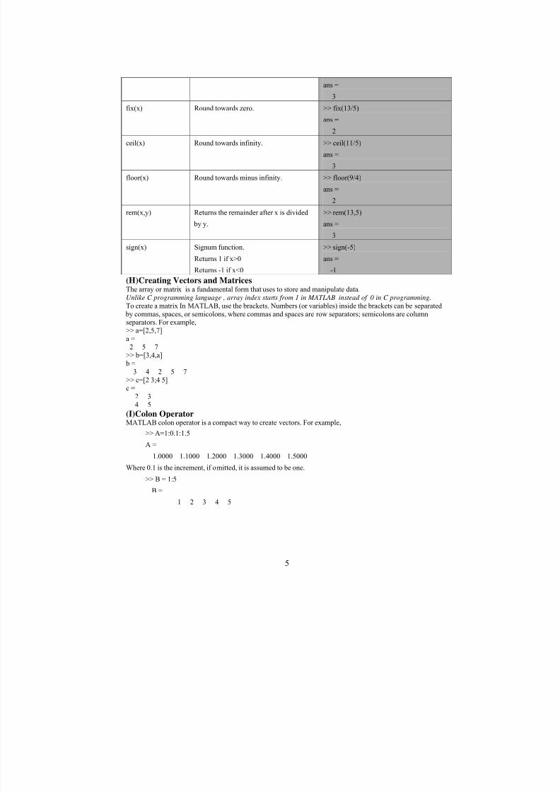
round(x) Round to the nearest integer >> round(17/5)



5

ans =

3

fix(x) Round towards zero. >> fix(13/5)ans =

2

ceil(x) Round towards infinity. >> ceil(11/5)

ans =

3

floor(x) Round towards minus infinity. >> floor(9/4)

ans =

2

rem(x,y) Returns the remainder after x is divided

by y.

>> rem(13,5)

ans =

3

sign(x) Signum function.

Returns 1 if x>0

Returns -1 if x<0

>> sign(-5)

ans =

-1

(H)Creating Vectors and MatricesThe array or matrix is a fundamental form that uses to store and manipulate data.

Unlike C programming language , array index starts from 1 in MATLAB instead of 0 in C programming.

To create a matrix In MATLAB, use the brackets. Numbers (or variables) inside the brackets can be separated

by commas, spaces, or semicolons, where commas and spaces are row separators; semicolons are columnseparators. For example,

>> a=[2,5,7]a =2 5 7

>> b=[3,4,a]

b =

3 4 2 5 7

>> c=[2 3;4 5]c =

2 3

4 5

(I)Colon OperatorMATLAB colon operator is a compact way to create vectors. For example,

>> A=1:0.1:1.5

A =

1.0000 1.1000 1.2000 1.3000 1.4000 1.5000

Where 0.1 is the increment, if omitted, it is assumed to be one.

>> B = 1:5

B =

1 2 3 4 5



6

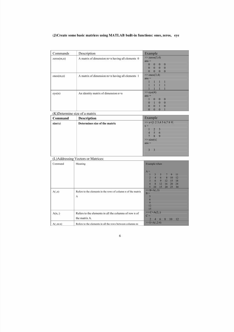
(J)Create some basic matrices using MATLAB built-in functions: ones, zeros, eye

Commands Description Example

zeros(m,n) A matrix of dimension m×n having all elements 0 >> zeros(3,4)

ans =

0 0 0 0

0 0 0 00 0 0 0

ones(m,n) A matrix of dimension m×n having all elements 1 >> ones(3,4)ans =

1 1 1 1

1 1 1 1

1 1 1 1

eye(n) An identity matrix of dimension n×n >> eye(4)ans =

1 0 0 0

0 1 0 00 0 1 0

0 0 0 1

(K)Determine size of a matrix

Command Description Example

size(x) Determines size of the matrix >> x=[1 2 3;4 5 6;7 8 9]

x =

1 2 3

4 5 6

7 8 9>> size(x)

ans =

3 3

(L)Addressing Vectors or Matrices:

Command Meaning Example when

A =1 3 5 7 9 11

2 4 6 8 10 123 6 9 12 15 18

4 8 12 16 20 245 10 15 20 25 30

A(:,n) Refers to the elements in the rows of column n of the matrix

A

>> B=A(:,3)B =

5

69

1215

A(n,:) Refers to the elements in all the columns of row n of

the matrix A.

>> C=A(2,:)

C =2 4 6 8 10 12

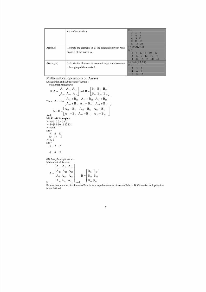
A(:,m:n) Refers to the elements in all the rows between columns m>> E=A(:,2:4)



7

and n of the matrix AE =

3 5 7

4 6 86 9 12

8 12 1610 15 20

A(m:n,:) Refers to the elements in all the columns between rows

m and n of the matrix A.

>> D=A(2:4,:)

D =2 4 6 8 10 12

3 6 9 12 15 18

4 8 12 16 20 24

A(m:n,p:q) Refers to the elements in rows m trough n and columns

p through q of the matrix A.

>> F=A(1:3,2:4)

F =

3 5 7

4 6 86 9 12

Mathematical operations on Arrays(A)Addition and Subtraction of Arrays :

Mathematical Review:

If ⎥⎦

⎤⎢⎣

⎡=

232221

131211

A A A

A A AA and ⎥

⎦

⎤⎢⎣

⎡=

232221

131211

B B B

B B BB

Then , ⎥⎦

⎤⎢⎣

⎡

+++

+++=+

BA BA BA

BA BA BABA

232322222121

131312121111

And,

⎥⎦

⎤⎢⎣

⎡

−−−

−−−=−

BA BA BA

BA BA BABA

232322222121

131312121111

MATLAB Example :

>> A=[1 2 3;4 5 6];>> B=[8 9 10;11 12 13];

>> A+B

ans =9 11 13

15 17 19

>> A-Bans =

-7 -7 -7

-7 -7 -7

(B) Array Multiplications :

Mathematical Review :

If

⎥⎥⎥⎥

⎦

⎤

⎢⎢⎢⎢

⎣

⎡

=

434241

333231

232221

131211

A AA

A AA

A A A

A A A

A

and⎥⎥⎥

⎦

⎤

⎢⎢⎢

⎣

⎡

=

3231

2221

1211

BB

B B

B B

B

Be sure that, number of columns of Matrix A is equal to number of rows of Matrix B .Otherwise multiplication

is not defined.



8

Then,

⎥⎥

⎥⎥

⎦

⎤

⎢⎢

⎢⎢

⎣

⎡

=

434241

333231

232221

131211

A AA

A AA

A A A

A A A

AB

⎥⎥⎥⎦

⎤

⎢⎢⎢⎣

⎡

3231

2221

1211

BB

B B

B B

=

⎥⎥⎥⎥

⎦

⎤

⎢⎢⎢⎢

⎣

⎡

++++

++++

++++

++++

324322421241314321421141

323322321231313321321131

322322221221312321221121

321322121211311321121111

BABABA BABABA

BABABA BABABA

BABABA BABABA

BABABA BABABA

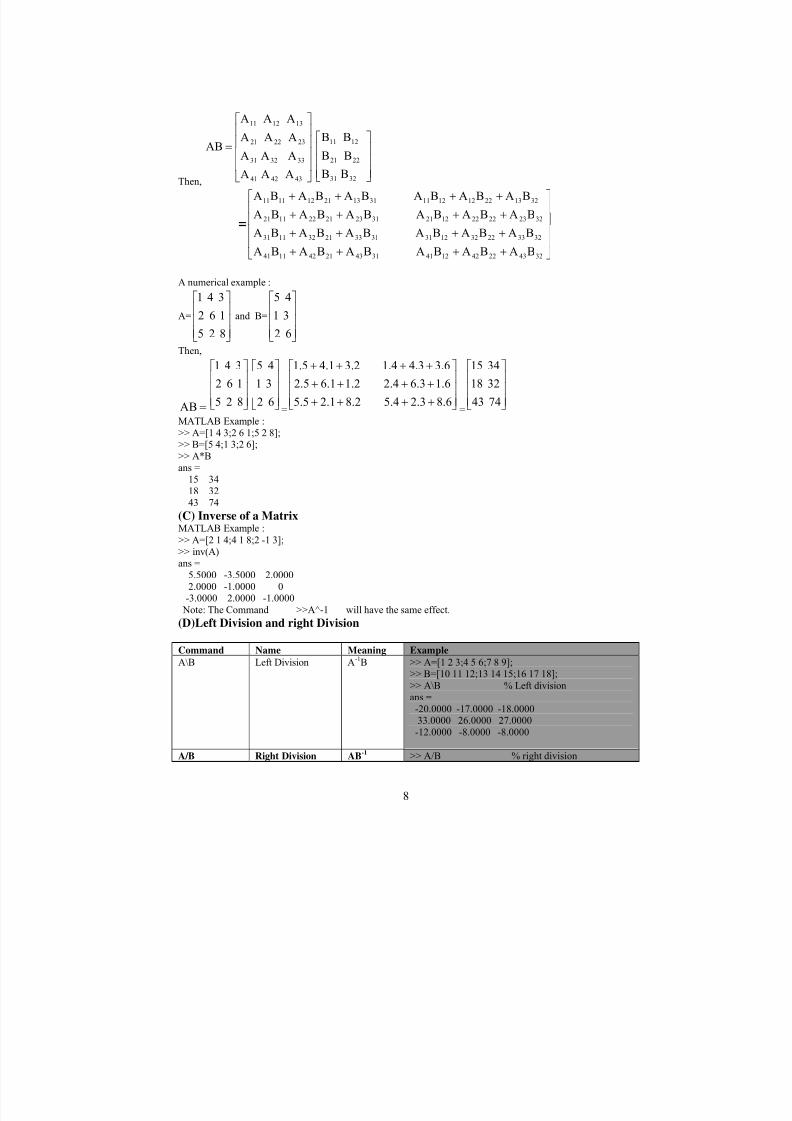
A numerical example :

A=

⎥⎥⎥

⎦

⎤

⎢⎢⎢

⎣

⎡

8 2 5

1 6 2

3 4 1

and B=

⎥⎥⎥

⎦

⎤

⎢⎢⎢

⎣

⎡

6 2

3 1

4 5

Then,

=AB⎥⎥⎥

⎦

⎤

⎢⎢⎢

⎣

⎡

8 2 5

1 6 2

3 4 1

⎥⎥⎥

⎦

⎤

⎢⎢⎢

⎣

⎡

6 2

3 1

4 5

=⎥⎥⎥

⎦

⎤

⎢⎢⎢

⎣

⎡

++++

++++

++++

8.62.35.4 8.22.15.5

1.66.32.4 1.26.12.5

3.64.31.4 2.31.45.1

=⎥⎥⎥

⎦

⎤

⎢⎢⎢

⎣

⎡

74 43

32 18

34 15

MATLAB Example :

>> A=[1 4 3;2 6 1;5 2 8];>> B=[5 4;1 3;2 6];

>> A*B

ans =15 34

18 32

43 74

(C) Inverse of a MatrixMATLAB Example :

>> A=[2 1 4;4 1 8;2 -1 3];

>> inv(A)ans =

5.5000 -3.5000 2.0000

2.0000 -1.0000 0-3.0000 2.0000 -1.0000

Note: The Command >>A^-1 will have the same effect.

(D)Left Division and right Division

Command Name Meaning Example

A\B Left Division A-1B >> A=[1 2 3;4 5 6;7 8 9];>> B=[10 11 12;13 14 15;16 17 18];

>> A\B % Left division

ans =

-20.0000 -17.0000 -18.000033.0000 26.0000 27.0000

-12.0000 -8.0000 -8.0000

A/B Right Division AB-1

>> A/B % right division



9

ans =

1.0000 3.0000 -3.0000

1.0000 2.0000 -2.0000

0.5000 2.0000 -1.5000

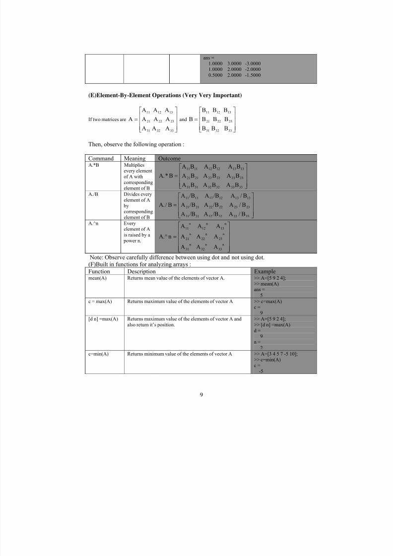
(E)Element-By-Element Operations (Very Very Important)

If two matrices are

⎥⎥⎥

⎦

⎤

⎢⎢⎢

⎣

⎡

=

333231

232221

131211

A AA

A A A

A A A

A and

⎥⎥⎥

⎦

⎤

⎢⎢⎢

⎣

⎡

=

333231

232221

131211

B BB

B B B

B B B

B

Then, observe the following operation :

Command Meaning OutcomeA.*B Multiplies

every element

of A with

corresponding

element of B⎥⎥⎥

⎦

⎤

⎢⎢⎢

⎣

⎡

=

333332323131

232322222121

131312121111

BA BA BA

BA BA BA

BA BA BA

B*.A

A./B Divides every

element of A

bycorresponding

element of B⎥⎥⎥

⎦

⎤

⎢⎢⎢

⎣

⎡

=

333332323131

232322222121

131312121111

B/A /BA /BA

B/A /BA /BA

B/A /BA /BA

B/.A

A.^n Every

element of Ais raised by a

power n.

⎥⎥⎥⎥

⎦

⎤

⎢⎢⎢⎢

⎣

⎡

=n

33

n

32

n

31

n

23

n

22

n

21

n

13

n

12

n

11

A A A

A A A

A A A

n.^A

Note: Observe carefully difference between using dot and not using dot.

(F)Built in functions for analyzing arrays :

Function Description Examplemean(A) Returns mean value of the elements of vector A. >> A=[5 9 2 4];

>> mean(A)ans =

5

c = max(A) Returns maximum value of the elements of vector A >> c=max(A)

c =9

[d n] =max(A) Returns maximum value of the elements of vector A and

also return it’s position.

>> A=[5 9 2 4];

>> [d n] =max(A)

d =9

n =

2

c=min(A) Returns minimum value of the elements of vector A >> A=[3 4 5 7 -5 10];

>> c=min(A)

c =

-5



10

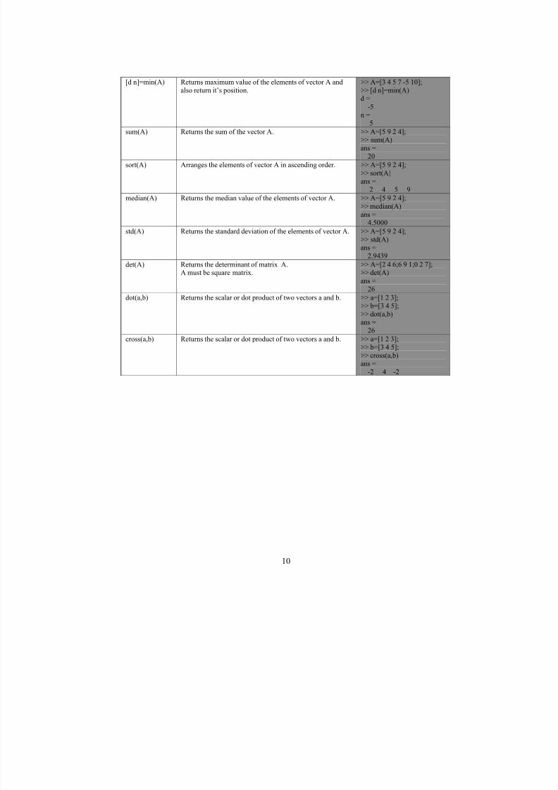
[d n]=min(A) Returns maximum value of the elements of vector A and

also return it’s position.

>> A=[3 4 5 7 -5 10];

>> [d n]=min(A)

d =

-5n =

5

sum(A) Returns the sum of the vector A. >> A=[5 9 2 4];>> sum(A)

ans =

20

sort(A) Arranges the elements of vector A in ascending order. >> A=[5 9 2 4];

>> sort(A)

ans =

2 4 5 9

median(A) Returns the median value of the elements of vector A. >> A=[5 9 2 4];

>> median(A)

ans =4.5000

std(A) Returns the standard deviation of the elements of vector A. >> A=[5 9 2 4];

>> std(A)ans =

2.9439

det(A) Returns the determinant of matrix A.A must be square matrix.

>> A=[2 4 6;6 9 1;0 2 7];>> det(A)

ans =

26

dot(a,b) Returns the scalar or dot product of two vectors a and b. >> a=[1 2 3];

>> b=[3 4 5];

>> dot(a,b)ans =

26

cross(a,b) Returns the scalar or dot product of two vectors a and b. >> a=[1 2 3];>> b=[3 4 5];

>> cross(a,b)

ans =

-2 4 -2



11

Script Files in MATLABWhy script Files :

In the previous session, the commands were executed in the command window. Although every MATLAB

command can be executed in this way, there are some drawbacks of using command window .

(i) Using the command window to execute a series of commands especially if they are related to eachother is not convenient and may be difficult or even impossible.

(ii) The commands in the command window cannot be saved and executed again.

(iii) The command window is not interactive. This means that, every time the ENTER key is pressed ,only the last command is executed, and everything executed before is unchanged. If a change or

correction is needed in a previous command ,the commands have to be entered again.

A different way of executing commands with MATLAB is first to create a file with a list of commands,

save it and then run the file. The files that are used for this purpose is called script files.

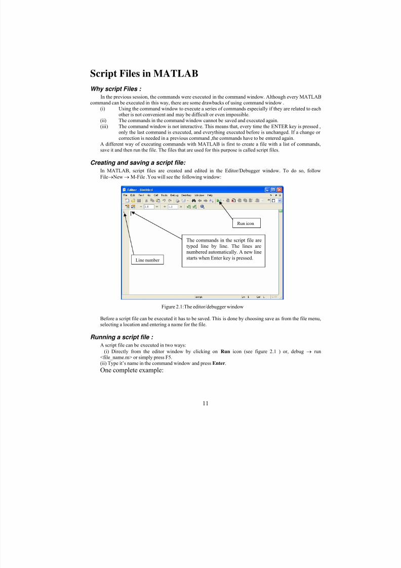
Creating and saving a script file:

In MATLAB, script files are created and edited in the Editor/Debugger window. To do so, follow

File→ New → M-File .You will see the following window:

Before a script file can be executed it has to be saved. This is done by choosing save as from the file menu,selecting a location and entering a name for the file.

Running a script file :

A script file can be executed in two ways:

(i) Directly from the editor window by clicking on Run icon (see figure 2.1 ) or, debug → run<file_name.m> or simply press F5.

(ii) Type it’s name in the command window and press Enter.

One complete example:

The commands in the script file are

typed line by line. The lines arenumbered automatically. A new line

starts when Enter key is pressed.Line number

Figure 2.1:The editor/debugger window

Run icon



12

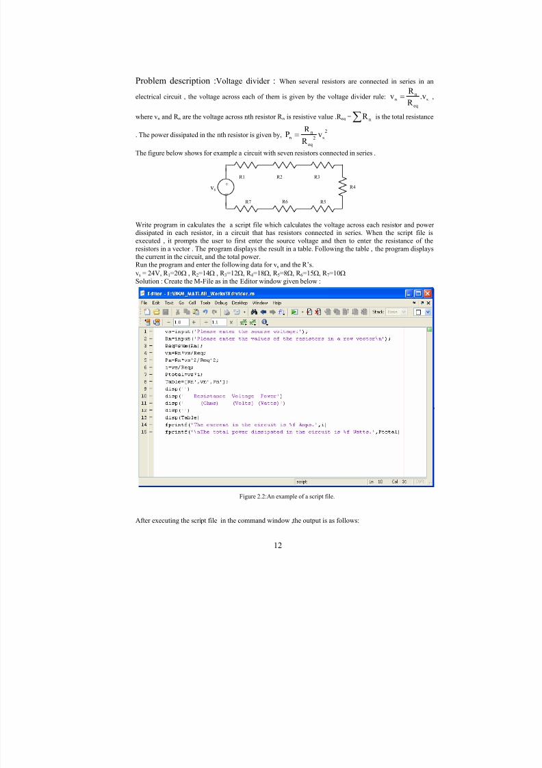
Problem description :Voltage divider : When several resistors are connected in series in an

electrical circuit , the voltage across each of them is given by the voltage divider rule: s

eq

nn v.

R

R v = ,

where vn and R n are the voltage across nth resistor R n is resistive value .R eq =∑ nR is the total resistance

. The power dissipated in the nth resistor is given by,2

s2

eq

nn v

R

R P =

The figure below shows for example a circuit with seven resistors connected in series .

Write program in calculates the a script file which calculates the voltage across each resistor and power dissipated in each resistor, in a circuit that has resistors connected in series. When the script file is

executed , it prompts the user to first enter the source voltage and then to enter the resistance of the

resistors in a vector . The program displays the result in a table. Following the table , the program displays

the current in the circuit, and the total power.Run the program and enter the following data for vs and the R’s.

vs = 24V, R 1=20Ω , R 2=14Ω , R 3=12Ω, R 4=18Ω, R 5=8Ω, R 6=15Ω, R 7=10Ω

Solution : Create the M-File as in the Editor window given below :

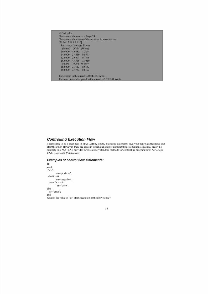
After executing the script file in the command window ,the output is as follows:

+

_

R1 R2 R3

R4

R7 R6 R5

vs

Figure 2.2:An example of a script file.



13

Controlling Execution Flow It is possible to do a great deal in MATLAB by simply executing statements involving matrix expressions, one

after the other, However, there are cases in which one simply must substitute some non-sequential order. To

facilitate this, MATLAB provides three relatively standard methods for controlling program flow: For Loops,While Loops, and If statements

Examples of control flow statements:

IF:

x=-3;

if x>0str=’positive’;

elseif x<0

str=’negative’;elseif x = = 0

str=’zero’;

else

str=’error’;

end

What is the value of ’str’ after execution of the above code?

>> Vdivider

Please enter the source voltage:24

Please enter the values of the resistors in a row vector [20 14 12 18 8 15 10]

Resistance Voltage Power

(Ohms) (Volts) (Watts)

20.0000 4.9485 1.2244

14.0000 3.4639 0.857112.0000 2.9691 0.7346

18.0000 4.4536 1.1019

8.0000 1.9794 0.489715.0000 3.7113 0.9183

10.0000 2.4742 0.6122

The current in the circuit is 0.247423 Amps.

The total power dissipated in the circuit is 5.938144 Watts.



14

WHILE:

x=-10;while x<0

x=x+1;endWhat is the value of x after execution of the above loop?

FOR loop:

X=0;

for i=1:10X=X+1;

end

The above code computes the sum of all numbers from 1 to 10.

SWITCH:X = 10;

switch x

case 5

disp (‘x is 5’)

case 6

disp (‘x is 6’)case 8

disp (‘x is 8’)

case 10disp (‘x is 10’)

otherwise

disp (‘invalid choice’)

end

BREAK:

The break statement lets you exit early from a for or a while loop:

x=-10;

while x<0

x=x+2;

if x = = -2 break;

end

end

MATLAB supports the following relational and logical operators:

Relational Operators: Symbol Meaning

< = Less than or equal to

< Less than> = Greater than or equal to

> Greater than

= = Equal to

˜ = Not equal to (unlike C. In C, it was !=)

Logical Operators: Symbol Meaning

& AND

| OR ˜ (tilde) NOT (unlike C. In C, it was !)



15

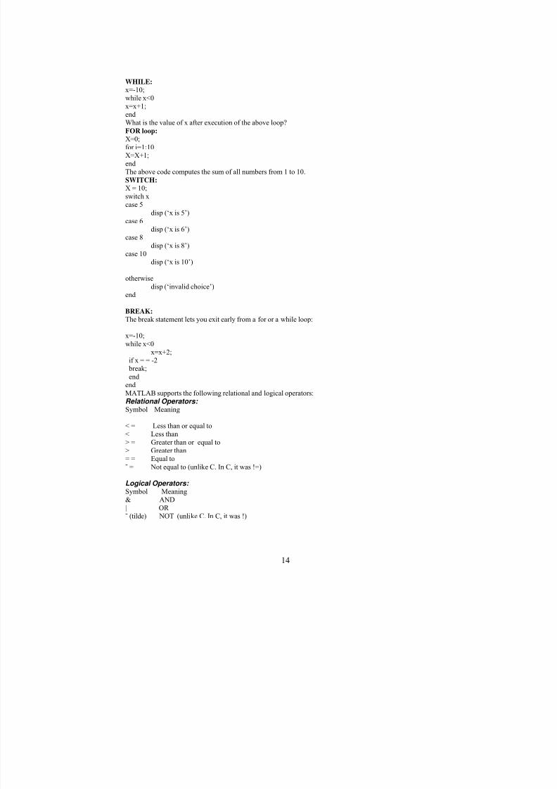
An Illustrative complete Example of using control flow : Example: Write a script file to sum the series 1+2+3+………….n , n taken from user.

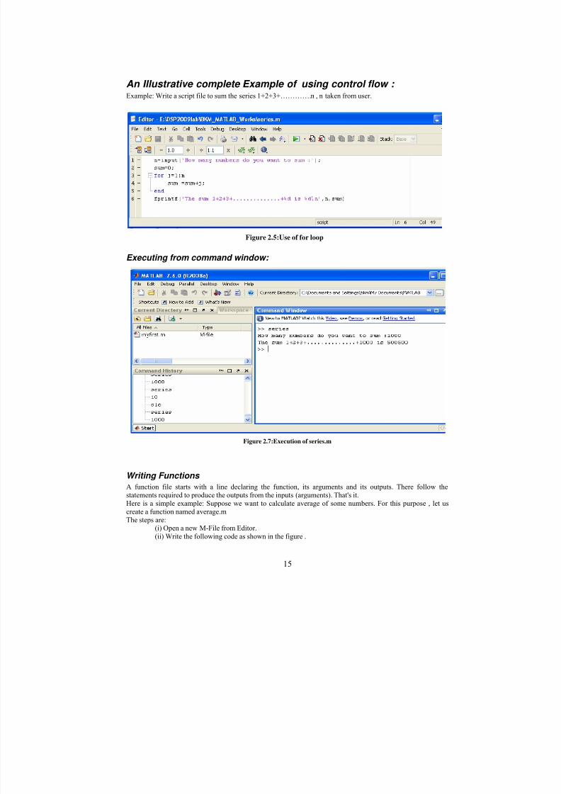
Executing from command window:

Writing Functions

A function file starts with a line declaring the function, its arguments and its outputs. There follow the

statements required to produce the outputs from the inputs (arguments). That's it.

Here is a simple example: Suppose we want to calculate average of some numbers. For this purpose , let us

create a function named average.m

The steps are:(i) Open a new M-File from Editor.

(ii) Write the following code as shown in the figure .

Figure 2.5:Use of for loop

Figure 2.7:Execution of series.m



16

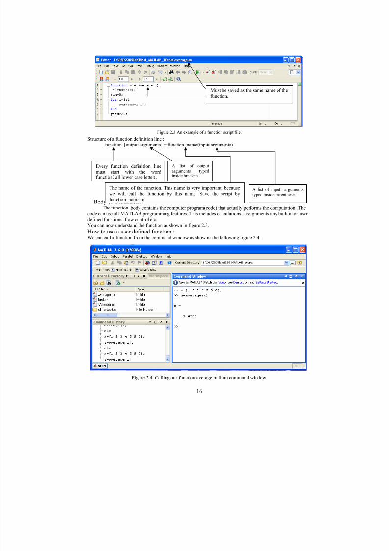
Structure of a function definition line :

function [output arguments] = function_name(input arguments)

Body of a function :The function body contains the computer program(code) that actually performs the computation .The

code can use all MATLAB programming features. This includes calculations , assignments any built in or user

defined functions, flow control etc.

You can now understand the function as shown in figure 2.3.

How to use a user defined function :We can call a function from the command window as show in the following figure 2.4 .

Must be saved as the same name of the

function.

Figure 2.3:An example of a function script file.

Every function definition line

must start with the wordfunction all lower case letter .

A list of outputarguments typed

inside brackets.

Figure 2.4: Calling our function average.m from command window.

The name of the function. This name is very important, because

we will call the function by this name. Save the script by

function name.m

A list of input argumentstyped inside parentheses.



17

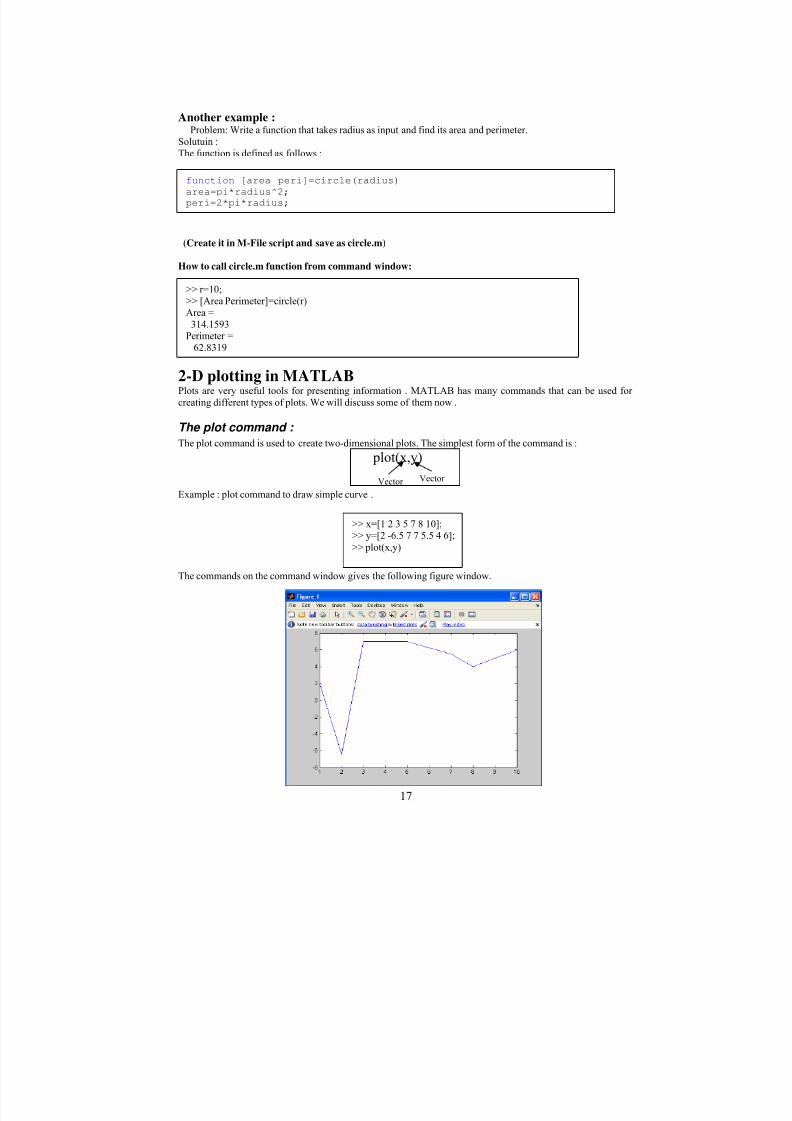
Another example :Problem: Write a function that takes radius as input and find its area and perimeter.

Solutuin :

The function is defined as follows :

(Create it in M-File script and save as circle.m)

How to call circle.m function from command window:

2-D plotting in MATLAB Plots are very useful tools for presenting information . MATLAB has many commands that can be used for

creating different types of plots. We will discuss some of them now .

The plot command :

The plot command is used to create two-dimensional plots. The simplest form of the command is :

plot(x,y)

Example : plot command to draw simple curve .

The commands on the command window gives the following figure window.

function [area peri]=circle(radius)

area=pi*radius^2; peri=2*pi*radius;

>> r=10;

>> [Area Perimeter]=circle(r)

Area =314.1593

Perimeter =

62.8319

Vector Vector

>> x=[1 2 3 5 7 8 10];>> y=[2 -6.5 7 7 5.5 4 6];

>> plot(x,y)



18

The plot command has additional optional arguments that can be used to specify the color and style of the line

and the color and type of markers,if any are desired.With these options the command has the form:

Line specifiers :Line specifiers are optional and can be used to define the style and color of the line and type of the markers (if

the markers are used).The line specifiers are:

Line style Specifier

solid(default) -

dashed --

dotted :

Dash-dott -.

Line color specifier :Line color Specifier red r

green g

blue b

cyan c

magenta m

yellow y

black k

white w

Marker type specifiers are :

Marker type Specifier

plus sign +circle o

asterisk *

point .square s

diamond d

five-point star p

six-point star h

Some examples :

Command Meaning plot(x,y) A blue solid line connecting the points with no markers (default)

plot(x,y,’r’) A red solid line connecting the points.

plot(x,y,’--y’) A yellow dashed line connecting the lines plot(x,y,’*’) The points are marked with * (no line between points)

plot(x,y,’g:d’) A green dotted line connecting the points that are marked with diamond markers.

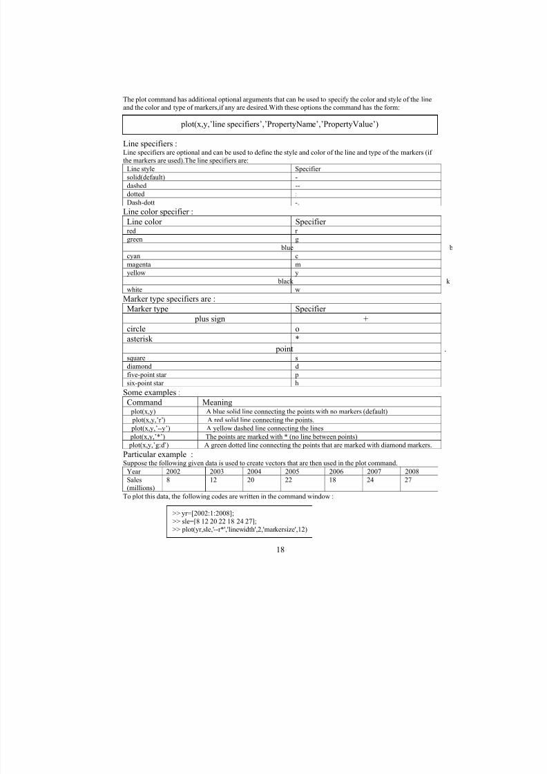
Particular example :Suppose the following given data is used to create vectors that are then used in the plot command.

Year 2002 2003 2004 2005 2006 2007 2008

Sales

(millions)

8 12 20 22 18 24 27

To plot this data, the following codes are written in the command window :

plot(x,y,’line specifiers’,’PropertyName’,’PropertyValue’)

>> yr=[2002:1:2008];

>> sle=[8 12 20 22 18 24 27];

>> plot(yr,sle,'--r*','linewidth',2,'markersize',12)



19

After execution the following figure window is opened.

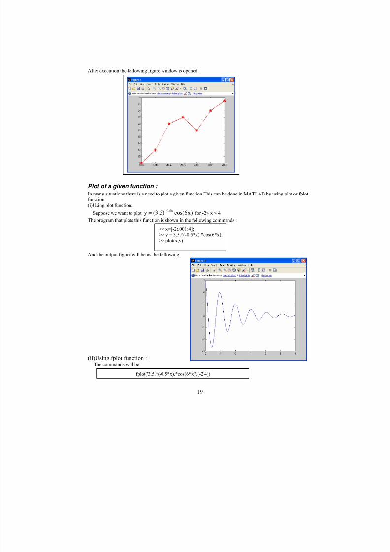
Plot of a given function :

In many situations there is a need to plot a given function.This can be done in MATLAB by using plot or fplot

function.

(i)Using plot function:

Suppose we want to plot )x6cos()5.3(y x5.0−= for -2≤ x ≤ 4

The program that plots this function is shown in the following commands :

And the output figure will be as the following:

(ii)Using fplot function :The commands will be :

>> x=[-2:.001:4];>> y = 3.5.^(-0.5*x).*cos(6*x);

>> plot(x,y)

fplot('3.5.^(-0.5*x).*cos(6*x)',[-2 4])



20

The output figure is the same as above.

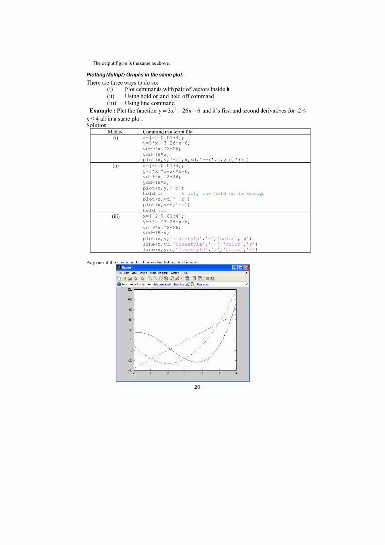
Plotting Multiple Graphs in the same plot: There are three ways to do so:

(i) Plot commands with pair of vectors inside it

(ii) Using hold on and hold off command(iii) Using line command

Example : Plot the function 6x26x3y 3 +−= and it’s first and second derivatives for -2 ≤

x ≤ 4 all in a same plot .Solution :

Method Command in a script file

(i) x=[-2:0.01:4];

y=3*x.^3-26*x+6;

yd=9*x.^2-26;ydd=18*x;

plot(x,y,'-b',x,yd,'--r',x,ydd,':k') (ii) x=[-2:0.01:4];

y=3*x.^3-26*x+6; yd=9*x.^2-26; ydd=18*x; plot(x,y,'-b') hold on % only one hold on is enough plot(x,yd,'--r') plot(x,ydd,':k') hold off

(iii) x=[-2:0.01:4]; y=3*x.^3-26*x+6; yd=9*x.^2-26; ydd=18*x; plot(x,y,'linestyle','-','color','b') line(x,yd,'linestyle','--','color','r') line(x,ydd,'linestyle',':','color','k')

Any one of the command will give the following figure:



21

Formatting a plot using commands :

The formatting commands are placed after the plot or fplot commands .The various formatting commands are

shown in the following table:

Labeling the axes :Forms Purposexlabel(‘string’)

ylabel(‘string’)

To label the x axis and y axis by text.

title(‘string’) To give a title to your figure

text(x,y,’ string’)gtext(‘string’)

To place a text anywhere on the figure.

legend(‘string1’,’string2’……) To place a legend on the plot.

Setting limits of axes :

Forms Purposeaxis([xmin , xmax]) Sets the limits of the x axis (xmin and xmax are numbers)

axis([xmin , xmax,ymin,ymax]) Sets the limits of both the axis

axis equal Sets the same scale for both the axisaxis square Sets the axis region to be square

Setting gridline on/off :

Forms Purposegrid on Adds grid line to the plot

grid off Removes grid line from the plot

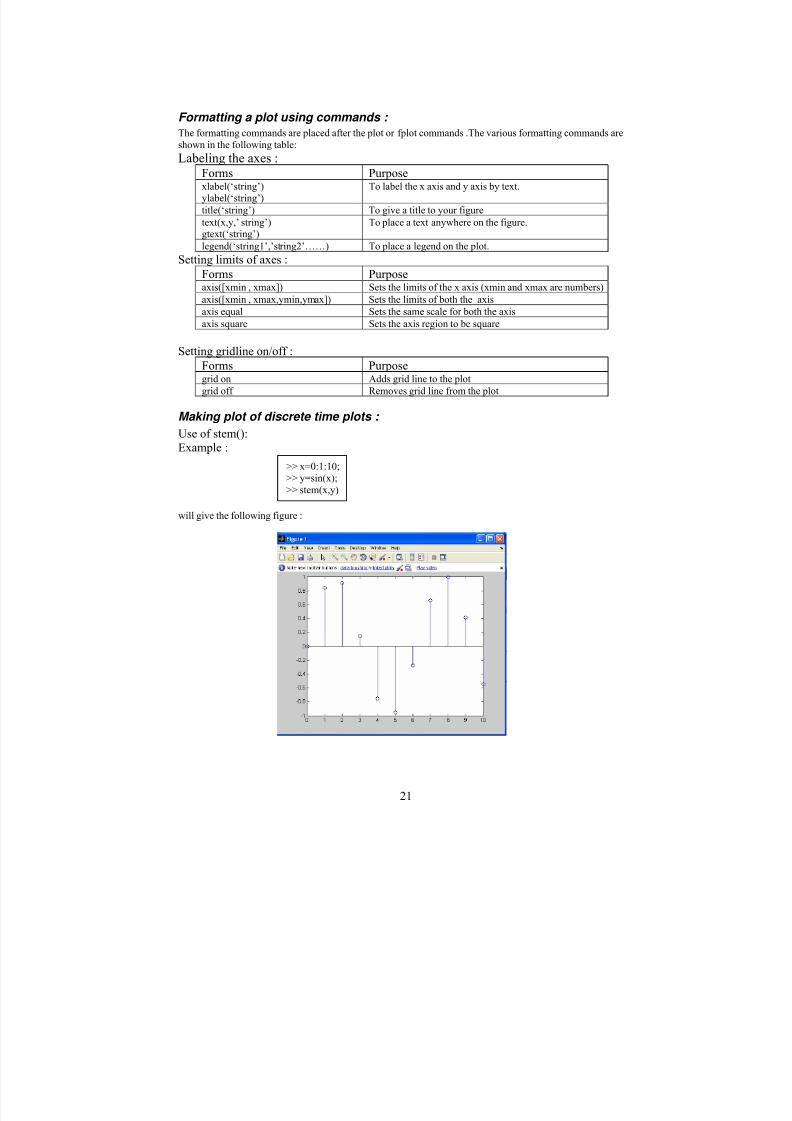
Making plot of discrete time plots :

Use of stem():Example :

will give the following figure :

>> x=0:1:10;>> y=sin(x);

>> stem(x,y)



22

Plotting Multiple plots on the same page :

Use of subplot :

Multiple plots on the same page can be created with the subplot command which has theformsubplot(m,n,p)

The command divides the figure window (page when printed) into m×n rectangular subplots

where plots will be created . p varies from 1 to m.n row wise. For examplesubplot(3,2,1)……..(3,2,6) will create the following arrangement.

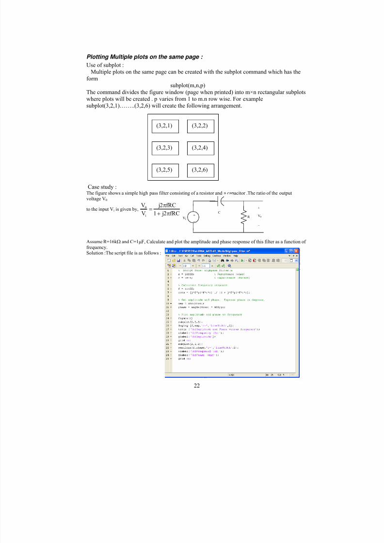
Case study :The figure shows a simple high pass filter consisting of a resistor and a capacitor .The ratio of the output

voltage V0

to the input Vi is given by,fRC2 j1

fRC2 j

V

V

i

0

π+π

=

Assume R=16k Ω and C=1µF, Calculate and plot the amplitude and phase response of this filter as a function of

frequency.Solution :The script file is as follows :

(3,2,1) (3,2,2)

(3,2,3) (3,2,4)

(3,2,5) (3,2,6)

+

_

C

R vi

+

V0

_



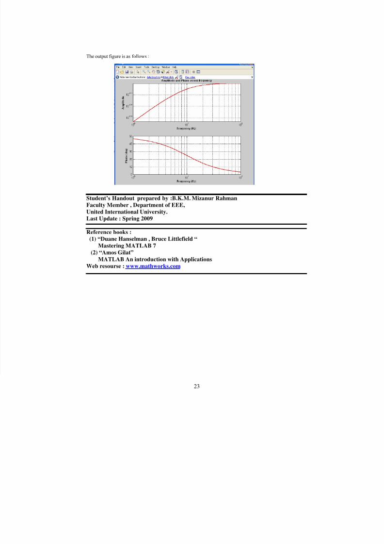
23

The output figure is as follows :

Student’s Handout prepared by :B.K.M. Mizanur Rahman

Faculty Member , Department of EEE,

United International University.

Last Update : Spring 2009

Reference books :

(1) “Duane Hanselman , Bruce Littlefield “

Mastering MATLAB 7

(2) “Amos Gilat”

MATLAB An introduction with Applications

Web resourse : www.mathworks.com

Documents

Eee Handout 2 Matlab