Eﬀect of size distribution on mixing of a polydisperse wet

Noname manuscript No.(will be inserted by the editor)

Effect of size distribution on mixing of a polydisperse wet

granular material in a belt-driven enclosure

Pallab Sinha Mahapatra · Sam Mathew ·

Mahesh V. Panchagnula · Srikanth Vedantam

the date of receipt and acceptance should be inserted later

Abstract We use a recently developed coupled fluid-particle discrete element

model to study mixing of a wet granular material in a two dimensional setting. The

particles are modeled as linearly elastic disks and are considered to be immersed

Pallab Sinha Mahapatra

Department of Applied Mechanics, Indian Institute of Technology Madras, Chennai 600 036

India.

Present address: Department of Mechanical and Industrial Engineering, University of Illinois

at Chicago, Chicago 60607 USA

E-mail: [email protected]

Sam Mathew · Mahesh V. Panchagnula

Department of Applied Mechanics, Indian Institute of Technology Madras, Chennai 600 036

India

E-mail: [email protected]; [email protected]

Srikanth Vedantam

Department of Engineering Design, Indian Institute of Technology Madras, Chennai 600 036

India

E-mail: [email protected]

2 Pallab Sinha Mahapatra et al.

in a Newtonian fluid. The fluid-particle interaction is modeled using a linear drag

model under the assumption that the fluid inertia is small compared to parti-

cle inertia. The granular slurry is driven by a belt moving at constant velocity

in a square cavity. In the simulations, we consider three types of size distribu-

tions: monodisperse, bidisperse with several particle size ratios, and polydisperse

Gaussian distributions with several different standard deviations. Mixing is char-

acterized using both strong and weak measures. Size segregation is observed only

in the bidisperse simulations. The energy required for mixing polydisperse slurries

decreases with increasing standard deviation of the particle sizes. Finally, we show

the benefits of engineering certain polydisperse particle size distributions towards

minimizing energy consumption.

1 Introduction

The flow of granular materials has been widely studied for several decades due to

their scientific and technological importance. Mixing and segregation in granular

flows is particularly important in many industrial applications. The role of size

polydispersity on mixing and segregation has been studied through experiments

[1] and by modeling [2]. An interstitial fluid such as air plays a minor role in

the mechanics of the dry granular flows [3–8]. On the other hand, an interstitial

fluid such as water or oil plays a significant role in the mechanics of wet granular

flows. While wet granular flows have been just as important from the industrial

viewpoint, there have been far fewer studies on the mixing of such materials. The

main reason for the paucity of such studies is the difficulty in coupling the fluid

and particle interactions in a tractable manner.

Title Suppressed Due to Excessive Length 3

The presence of a small amount of liquid within the granular material only

increases the cohesive forces in the granular system [9]. On the other hand, if the

grains are fully immersed due to a larger amount of the liquid, the wet granular

material is called a slurry [10]. Fully immersed wet granular slurry flows occur

in the food industry, geological flows and in construction. In some industrial sec-

tors like chocolate and pharmaceuticals manufacturing, the flows may be in the

presence of a highly viscous interstitial fluid.

Several experimental studies have investigated the dynamics of wet granular

materials. Granular slurries have been studied in a 2D vibrated bed [9, 11], as

flows down inclines [12] and in circular rotating drums [13, 14]. With the decrease

of the volume of interstitial liquid, the role of liquid viscosity is greatly altered.

There have been fewer studies of the mechanics of such dense wet granular flows.

Models of granular slurries have been proposed by considering one-way coupling

[15, 16] and two-way coupling between the interstitial fluid and the particles [13].

The flow of granular particles in a lid driven cavity has also been studied in [17, 18].

Numerical studies of slurry flows have been generally few in number due to the

complexity in modelling coupled fluid-particle behavior. Recently, Bonkinpillewar

et al. [19] have developed a simple and computationally tractable model of wet

granular systems. The validity of the model is restricted to regimes where the

fluid inertia is small compared to the particle inertia in any representative volume

element. This assumption is satisfied in dense granular slurries in which the particle

density is large compared to the fluid density and thus encompasses many flows

of practical interest.

In this work we have considered a 2D system with an expectation that

the basic behavior will not change for 3D systems with unidirectional belt


motion. During simulations or processing images of experiments, most re-

searchers assume mixing to be a 2D phenomenon. When the third dimen-

sion is small (of the order of the particle diameter) and the driving con-

ditions are such that secondary flows are not induced, we consider the 2D

setting to be realistic. The dynamics of mixing and segregation of a binary

mixture of glass beads and coriander seeds were studied by Rodriguez et

al. [20] in a quasi 2D pile. They have assumed that the grains were layered

uniformly in all radial direction of the 3D pile. Misra and Poorsolhjouy [21]

studied the instability and stress-strain behavior of cylindrical particles in

2D regular assemblies. The width of the plate was taken small during the

experiment and hence they have assumed a 2D framework for their model-

ing. Hsiau et al. [11] experimentally investigated the effects of the addition

of liquid content, viscosity, and surface tension on dynamic properties of

wet particulates in a 2D wet vibrated granular bed. On the other hand,

when there exists an open surface and the flow front changes its direction

spontaneously researchers have considered 3D system, for example, particle

fluid motion in a rotating drum [22–24].

In industrial applications, granular materials are usually polydisperse. In addi-

tion, segregation of particles in polydisperse mixtures often occurs during handling

or transportation and can lead to undesired product quality. Segregation of par-

ticles can happen due to differences in particle sizes and other physical properties

which may affect the behavior of the granular flows. There is great interest in

analyzing the segregation processes in different geometries [4]. The effect of size

distribution of polydisperse granular flows has been found to be very important in

dry granular flows. Experiments by Jain et al. [25] indicate that enhanced mixing


and reduced segregation occur in binary and ternary mixtures with a size dis-

tribution of the particles. The amount of segregation has also been observed to

reduce with an increase of mass fraction of intermediate species present in the

system. Pereira and Cleary [14] studied the segregation of mixtures composed of

dry particles having either different sizes or density in rotating tumblers. Mixing

and segregation of multi component dry mixtures has also been reported by refer-

ences [6, 8]. DEM models have been used to simulate the mixing of bidisperse dry

granular particles as well as polydisperse dry granular flows [26, 27]. As mentioned

earlier, such extensive studies have not been performed in slurry flows.

In the present work we employ a DEM proposed by Bonkinpillewar et al. [19]

to study mixing of mono- and poly-disperse wet granular materials in a square

cavity. The grains are modeled as soft disks and the elastic collision between the

grains are assumed to follow the Hertz model. The fluid medium exerts a linear

drag on the particles which is taken to be proportional to the relative velocity of

the particle and the fluid medium at the particle location. Due to the assumption

that the fluid inertia is small compared to the particle inertia in any representative

area element, the velocity of the fluid is calculated as a weighted average of the

particle velocities in a neighborhood. A detailed description of the method can be

found in [19]. The present work deals with modeling the dynamics of dense

granular slurries (near the random packing limit). The inter particle colli-

sion time interval in such a system is small and solving the hydrodynamics

while accounting for the collisions is still computationally prohibitive. Our

modeling approach is intended to fill this gap and allows the user to perform

device-scale simulations. For large scale parametric studies, we hope that

this model will prove useful to designers with the exception of low volume


concentrations. In this work we have focused on understanding the mixing

of mono-disperse, bidisperse and polydisperse wet granular particles in a

lid driven enclosure. The polydisperse system is taken to contain uniform

size distribution and Gaussian distributions. To the best of author’s knowl-

edge the effect of polydispersity on wet granular mixing inside a belt driven

enclosure has not been studied before. In the following section, the equations

governing the model are briefly described following [19] and the numerical solu-

tion procedure is described in detail. Two measures of mixing are considered and

described in Sec. 2. The results of the simulations are presented in Sec. 3. The

monodisperse, bidisperse and polydisperse results are presented in juxtaposition

for comparison.

2 Numerical approach details

2.1 Model description

In this section, we briefly summarize the model presented in Bonkinpillewar et al.

[19]. The model is applicable to fully immersed wet granular slurries. The fluid

medium is considered to be viscous and the fluid inertia is assumed to be small

in comparison to the particle inertia. The model incorporates the interaction of

particles with each other and with the walls through Hertzian contact forces [28]

which, in a two dimensional setting, is a linear soft sphere model. The particles

experience a drag due to the fluid medium which is modeled by Stokes’ drag and is

taken to be linearly proportional to velocity of the particle relative to the velocity of

the fluid medium at that point. The velocity of the fluid is not explicitly calculated,

but is taken to be a weighted average of the surrounding particle velocities [29]. In


addition, a uniform gravity field is simulated by a constant force applied to each

particle, directed vertically downwards.

The total force on a particle is given by

F = Fpp + Fd +mg (1)

The interparticle interaction force (Fpp) is taken to be of a linear soft-sphere

form

Fpp =

−knδ |δ| > 0

0 otherwise

(2)

where δ =(∣

∣ri − rj∣

∣− ((di + dj)/2))

ri−rj

|ri−rj |, is the separation of two particles i

and j in terms position vectors ri and rj and diameters di and dj). The direction

of the force on a given particle is along the line joining the particle centers. The

coefficient kn is related to the elastic modulus of the particle material using Hertz

theory.

The equation for drag on a particle (i) is motivated by Stokes’ drag and taken

to be proportional to relative velocity between a particle and the fluid at the same

location [30].

Fd,i = Cvdi (vp,i − vi) (3)

where, Cv is a hydrodynamic drag coefficient similar to the drag coefficient 3πµ

of the Stokes’ law (µ is the fluid viscosity), vi is the velocity of particle i and

vp,i is the velocity of the surrounding fluid determined from a weighted mean of

surrounding particles. The relative velocity is determined using a newly proposed

weighted function based on n neighboring particles surrounding the ith particle:

vp,i =

∑n

j=1mjWij

(∥

∥ri − rj∥

∥ , hi)

vj∑n

j=1mjWij

(∥

∥ri − rj∥

∥ , hi) (4)


where the weighing function Wij is a Gaussian given by

Wij =

exp(

−η ‖ri−rj‖2

hi2

)

‖ri−rj‖hi

≤ 1

0 otherwise

(5)

and hi is a radius of influence for particle i which corresponds to the extent to

which the particle’s neighborhood influences its surrounding fluid velocity. Finally,

mi is the mass of the ith particle. In this study, we set h = 5d. A constant η

defines the standard deviation of the Gaussian distribution and is taken as 2 in

our simulations as suggested by Drumm et al. [29]. The calculated fluid velocity,

vp,i is taken to be zero if there are no surrounding particles in the neighborhood.

This is consistent with the assumption that fluid inertia is small in comparison to

particle inertia.

2.2 Simulation details

The simulations in this work are in a two dimensional square domain of side 40 cm.

Disks of diameter 5 mm are initially packed at 74% area fraction in a square lattice.

The walls of the domain are modeled by fixed disks of the same size as the particles.

In the monodisperse case, the domain is filled with 6084 particles. Three cases are

considered for the bidisperse simulations by introducing a second set of particles

of diameter 2.5 mm at different number concentrations (5%, 25% and 50%). In

the polydisperse case, particles with uniform size distribution and Gaussian size

distributions are considered with a mean diameter dm = 5 mm. Different cases

with standard deviations σ were considered, with σ/dm values ranging from 1% to

10%. In all the simulations the same packing fraction was maintained. The belt

driving the flow is placed at the bottom of the cavity and is composed of particles


of the same size as the granular particles. These belt particles are collectively

moved at a constant speed.

The equations of motion based on the algebraic sum of the forces on each

particle are solved numerically for the position and velocity as a function of time

using the Velocity-Verlet algorithm [31]. The three steps in the Velocity-Verlet

algorithm are

1. Position update: x(t+∆t) = x(t) + v(t)∆t+ 12a(t)∆t

2

2. New acceleration: a(t + ∆t) = Fnet(t+∆t)m , using the new position, x(t + ∆t),

from step 1

3. Velocity update: v(t+∆t) = v(t) + 12 [a(t) + a(t+∆t)]∆t

In the above algorithm, determining the forces on the particles at each time

step is the most computationally intensive part. According to the Velocity-Verlet

algorithm, the force on each particle needs to be calculated twice at each time

step. A linked list algorithm is employed to reduce the computational effort [32]

and to obtain accurate solutions.

2.3 Mixing and order quantification

Doucet et al. [33] have proposed weak and strong sense mixing parameters (βws and

βss, respectively) based on the degree of correlation of current particle positions

with respect to each of their initial coordinates (spatial and/or size dimensions).

The weak sense mixing parameter (βws) only depends on the particle position

relative to its initial location. For weak sense mixing, the distribution of particles

at time t is independent of the initial distribution. As such, the two distributions

are not correlated. On the other hand, the parameter quantifying mixing in the


strong sense βss includes the effect of particle sizes. In other words, it means that

the distribution of particles at time t is independent of the initial distribution with

respect to both space and properties. These parameters are determined based on

a Principal Component Analysis (PCA) of the particle positions and size data.

The detailed procedure for these mixing indices has been explained by Doucet

et al. [33]. The particles in the current problem are described by two spatial co-

ordinates and one size coordinate. Following Doucet et al. [33], we describe the

determination of the mixing indices

1. The particles positions and diameter coordinates at initial instant, t = 0 are

scaled based on the variance and mean.

2. The particles positions and diameter coordinates at future instants of time, t

are scaled based on the instantaneous variance and mean.

3. Computing the correlation matrix ρ(Xit, Xj

0), where i = 1,2, and j = 1, 2, 3.

X1 and X2 is the list of x and y coordinates of the particles and is a N-row

matrix (N being the number of particles),X3 corresponds to the size dimension.

By definition, the correlation matrix involves the product of the transpose of

(Xit) and (Xj

0), t and 0 denoting time instants.

4. Creating the correlation matrix C, by assigning Cij = ρ(Xit, Xj

0).

5. Computing matrix M , such that, M = CCT . M is now a symmetric matrix

6. Determining forM , the maximum eigenvalue λ and the corresponding eigenvec-

tor α. The solution of the eigenvalue problem αM = λα allows the construction

of eigenvectors.

7. The weak sense mixing parameter for two-dimensional space is defined as,

βws =√

λws/2 (6)


where λws corresponds to the eigenvalue of the matrixM , which is constructed

from the correlation matrix C, such that, Cij = ρ(Xit, Xj

0), and i, j = 1, 2,

i.e., only spatial correlation is considered. The weak sense mixing parameter

therefore, misses the size segregation effects.

8. The strong sense mixing parameter for two-dimensional space and additional

size coordinate is defined as,

βss =√

λss/3 (7)

λss corresponds to the eigenvalue of the matrix M , which is constructed from

the correlation matrix C, such that, Cij = ρ(Xit, Xj

0), and i = 1, 2, while

j = 1, 2,3, as described above.

The fluidity of the granular material has been quantified based on so-called

local and global order parameters proposed by Mermin [34]. The local order pa-

rameter is based on the polar orientation of the neighboring particles surrounding

a given particle. The local order parameter ψi for a particle i is given by

ψi =

∑nnb

k=1 ej6α

nnb=

1

nnb

nnb∑

k=1

[cos(6α) + j sin(6α)] (8)

where nnb is the number of neighbors in contact with the ith particle, j =√−1, and

α is the angle of the line segment joining the particle and its neighbor’s centers,

with respect to the X-axis. The overall local order parameter is represented in

this work purely as the magnitude of ψi. The global order parameter (Ψ) is the

average of the local order parameters over all the particles in the domain and is

correlated to the dilation boundaries in the domain. Higher values of the global

order parameter suggest better packing with respect to the neighboring particles.


3 Results and Discussion

We discuss the results of exercising the model discussed in the previous section

hereunder. The results are classified into three parts, (a) Mixing of monodisperse

particles, (b) Mixing of bidisperse particles and (c) Mixing of polydisperse parti-

cles.

3.1 Flow patterns and mixing process

3.1.1 Mixing of mono disperse particles

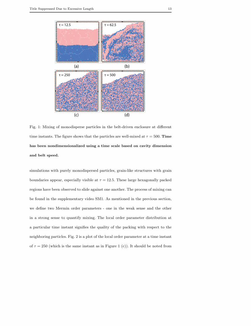
The patterns emerging from mixing monodisperse wet particles are shown in Fig.

1 for different time instants. The belt is impulsively started with a velocity of 0.5

after an initial gravitational settling time of τ = 12.5. τ is dimensionless time based

on the time scale associated with the belt motion. During this time, the particles

settle into a nearly crystalline packing. In order to identify the patterns, we have

colored the particles with two different colors (top half of the particles are colored

in pink while the bottom half are colored blue). Due to the motion of the belt, the

particles near the belt are initiated into motion by the belt. These particles subse-

quently collide with the particles away from the belt and transfer their momentum.

In addition, they collide with the side walls of the enclosure resulting in upward

motion before tumbling. These processes can be seen in Fig. 1(b) at τ = 62.5 where

the blue particles are surrounded by the pink particles; however, stratification can

still be observed. As time progresses, the particles are further mixed, resulting in

a nearly well mixed state by the time instant of about τ = 500. The belt-driven

enclosure exhibits flow patters reminiscent of the lid-driven cavity. In the current


τ = 12.5 τ = 62.5

τ = 250 τ = 500

(a) (b)

(c) (d)

Fig. 1: Mixing of monodisperse particles in the belt-driven enclosure at different

time instants. The figure shows that the particles are well-mixed at τ = 500. Time

has been nondimensionalized using a time scale based on cavity dimension

and belt speed.

simulations with purely monodispersed particles, grain-like structures with grain

boundaries appear, especially visible at τ = 12.5. These large hexagonally packed

regions have been observed to slide against one another. The process of mixing can

be found in the supplementary video SM1. As mentioned in the previous section,

we define two Mermin order parameters - one in the weak sense and the other

in a strong sense to quantify mixing. The local order parameter distribution at

a particular time instant signifies the quality of the packing with respect to the

neighboring particles. Fig. 2 is a plot of the local order parameter at a time instant

of τ = 250 (which is the same instant as in Figure 1 (c)). It should be noted from


this figure that wet granular materials tend to pack into a crystalline arrangement

with a few grain boundaries separating large oriented islands. In the present work

this kind of situation is observed only for monodispersed particles. The dilation of

such islands is one of the major processes through which monodisperse granular

material mixes. The energy transfer from the belt to regions in the granular mate-

rial away from the belt is facilitated by the transfer of force from the belt [35]. This

process can be visualized using force lines. Force lines are lines drawn through the

centers of the particles which are in direct contact with each other. The length

of these lines is an indication of the extent of influence of a given particle. In the

case of monodisperse particle systems, these lines appear to extend all the way

into the cavity owing to the fact that most of the material is closely packed in an

orderly arrangement. Therefore, the motion of the belt is both kinematically and

kinetically transferred to the regions away from the belt.

3.1.2 Mixing of bidisperse particles

We now turn our attention to the processes underlying mixing of bidisperse matieral.

The mixing of bidisperse particles is shown in Fig. 3 (which is similar to Fig. 1 for

the monodisperse case). The overall area fraction of the granular material in the

cavity in the bidisperse case is maintained the same as in the previous monodis-

perse case. The diameter ratio of the smaller particle to the larger particle is 0.5. In

addition, the number fraction of the secondary particles (smaller diameter) is 25%.

In Fig. 3(b) and (c) the particles are colored by Mermin’s local order parameter

[34] and by velocity (scaled with belt speed) respectively. The secondary particles

of a smaller size are shown as red particles in Fig. 3(a), and as black particles in

Fig. 3(b) and (c).


0 0.2 0.4 0.6 0.8 1

τ= 250

Fig. 2: Mermin’s local order parameter [34] variation for monodisperse system.

Particles are coloured by local order parameter [34] (values range from 0

(fluid, loosely packed) to 1 (solid, close packed). The figure shows the quality

of packing with grain boundaries. The white zones shows the voids inside the

closely packed particles.

Three observations can be drawn from this figure. Firstly, the mixture compo-

sition shown in Fig. 3(a) is significantly better mixed than that shown for monodis-

perse particles in Fig. 1 at the same time of τ = 250. Secondly, from comparing

the Mermin order parameter distribution in Fig. 3(b) to Fig. 2, one can observe

that the introduction of the smaller particles appears to break up the long range

close-packed structures that were prominent in Fig. 2. The granular matter, under

these circumstances, appears to take on a fluidized state which can be seen both

in Fig. 3(b) and (c). Fig. 3(c) shows a contour plot of the instantaneous velocity

field in the cavity. Lastly, three distinct regions can be observed in Fig. 3(c). A

high shear zone can be observed near the belt, a low shear zone (yellow region) can

be identified near the right wall of the cavity and a free flowing, cascading layer


0 0.2 0.4 0.6 0.8 1 0 0.02 0.04 0.06 0.08 0.1 0.12 0.14 0.16

(a) (b) (c)

Fig. 3: Particles in the belt-driven enclosure at τ = 250. Bidisperse system, number

fraction of secondary particles, n/N = 0.25 and d/D = 0.5. (a) Vertically stratified

layers mixing; (b) Particles coloured by Mermin’s local order parameter [34] (val-

ues range from 0 (fluid, loosely packed) to 1 (solid, close packed)); (c) Particles

coloured by speed contours (scaled with belt speed). The figure shows that after

adding the secondary particles the system becomes more fluid-like with less void

zones and closely packed structures. Three different fluid zones can be identified

from Fig. 3(c): high shear zone near the belt, no flow core zone of the rotating

particles and almost stagnant layers of particles above the circulating cell.

of particles can be seen on the free surface. These cascading particles are moving

much slower and exhibit much lower shear than the particles near the belt. Owing

to these observations, one can conclude that the introduction of a smaller particle

tends to promote fluidization in bidisperse granular material. However, an unin-

tended effect of this fluidization is that the force lines in the bidisperse case could

be shorter than in the monodisperse case. This results in less effiicient kinematic

transfer of wall momentum into the granular material.


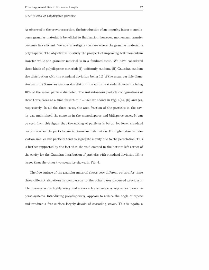
3.1.3 Mixing of polydisperse particles

As observed in the previous section, the introduction of an impurity into a monodis-

perse granular material is beneficial to fluidization; however, momentum transfer

becomes less efficient. We now investigate the case where the granular material is

polydisperse. The objective is to study the prospect of improving belt momentum

transfer while the granular material is in a fluidized state. We have considered

three kinds of polydisperse material: (i) uniformly random, (ii) Gaussian random

size distribution with the standard deviation being 1% of the mean particle diam-

eter and (iii) Gaussian random size distribution with the standard deviation being

10% of the mean particle diameter. The instantaneous particle configurations of

these three cases at a time instant of τ = 250 are shown in Fig. 4(a), (b) and (c),

respectively. In all the three cases, the area fraction of the particles in the cav-

ity was maintained the same as in the monodisperse and bidisperse cases. It can

be seen from this figure that the mixing of particles is better for lower standard

deviation when the particles are in Gaussian distribution. For higher standard de-

viation smaller size particles tend to segregate mainly due to the percolation. This

is further supported by the fact that the void created in the bottom left corner of

the cavity for the Gaussian distribution of particles with standard deviation 1% is

larger than the other two scenarios shown in Fig. 4.

The free surface of the granular material shows very different pattern for these

three different situations in comparison to the other cases discussed previously.

The free-surface is highly wavy and shows a higher angle of repose for monodis-

perse systems. Introducing polydispersity, appears to reduce the angle of repose

and produce a free surface largely devoid of cascading waves. This is, again, a


(a) (b) (c)

Fig. 4: Polydisperse particles in the belt-driven enclosure at τ = 250. (a) Uni-

form polydispersed particles with dmin = 2mm and dmax = 10mm; (b) Gaussian

distribution of particles with standard deviation 1%; (c) Gaussian distribution of

particles with standard deviation 10%. The figure shows that the segregation of

particles are different in different conditions whereas, the stable free surface can

be observed for uniform polydisperse and Gaussian distribution of particles for

standard deviation of 10%.

direct consequence of increased fluidization. Within the three polydisperse cases,

the free surface is more unsteady for the 1% standard deviation case shown in

Fig. 4(b), since it is the closest to the monodisperse case. The typical mixing of

polydisperse particles distributed in the uniformly random fashion can be seen

from the supplementary video SM2.

3.2 Quantification of mixedness and crystallinity

We have thus far, presented a qualitative picture of the mixing process. We would

like to quantify mixing in order to understand the expense incurred in the mixing

process, in terms of time and energy. From the previous discussion, it can be con-

cluded that the overall mixing occurs mainly in three stages, namely, tumbling,

inter-penetration and advection. In the tumbling phase, the initially stratified ma-


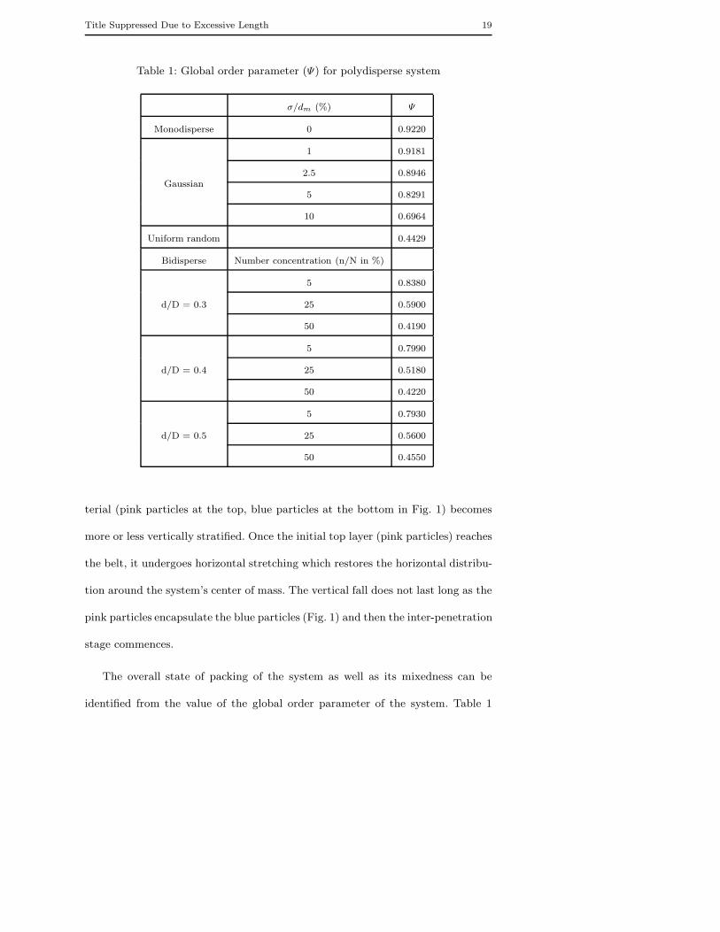
Table 1: Global order parameter (Ψ) for polydisperse system

σ/dm (%) Ψ

Monodisperse 0 0.9220

Gaussian

1 0.9181

2.5 0.8946

5 0.8291

10 0.6964

Uniform random 0.4429

Bidisperse Number concentration (n/N in %)

d/D = 0.3

5 0.8380

25 0.5900

50 0.4190

d/D = 0.4

5 0.7990

25 0.5180

50 0.4220

d/D = 0.5

5 0.7930

25 0.5600

50 0.4550

terial (pink particles at the top, blue particles at the bottom in Fig. 1) becomes

more or less vertically stratified. Once the initial top layer (pink particles) reaches

the belt, it undergoes horizontal stretching which restores the horizontal distribu-

tion around the system’s center of mass. The vertical fall does not last long as the

pink particles encapsulate the blue particles (Fig. 1) and then the inter-penetration

stage commences.

The overall state of packing of the system as well as its mixedness can be

identified from the value of the global order parameter of the system. Table 1


presents the average global order parameter for all the situations considered in the

present work. It may be recalled that a value of Ψ close to 1 indicates a nearly

crystalline (least fluidized) arrangement of the material. As can be noted from the

values in Table 1, the system exhibits the highest degree of crystalline packing

for the case of a monodisperse particles. Among the bidisperse situations, the

global order parameter decreases with an increase in the number concentration

(n/N) of the secondary particles. For a constant number concentration, Ψ also

appears to decrease with an increase in d/D (except for the very high values of

n/N). For the polydisperse situation, the lowest value of Ψ is observed in the

uniform polydisperse situation. From these observations, it can be concluded that

the presence of secondary particles makes the system less crystalline, resulting in

an enhanced fluidization.

The mechanism of enhanced fluidization in the bidisperse and polydisperse

cases deserves further discussion. As the bottom belt moves, flow structures similar

to separation bubbles in the classical lid-driven cavity become visible in the do-

main. While this may promise better mixing, segregation effects dominate in these

situations. Our results show that while adding secondary particles of a different

size aids in the initial stages of mixing by breaking up the crystalline structure. At

later times, large segregated zones appear (Fig. 3(b)), which result in an overall

poorer state of mixedness. In addition, the mixing which is driven by force line

propagation [36, 37] away from the belt become shorter in length. For these two

reasons, the initial advantage from enhanced fluidization disappears at later times,

especially for high concentrations of the secondary particles.

We now revisit the concept from mixedness by taking both particle size and

location into account. For this purpose, the strong mixing parameter is defined


βss

102 1051041030

0.2

0.4

0.6

0.7

0.1

0.3

0.5

n/N=5%Monodispersed/D=0.3d/D=0.4d/D=0.5

E

(a)

102 105104103

βss

0

0.2

0.4

0.6

0.7

0.1

0.3

0.5


E

(b)

102

βss

0

0.2

0.4

0.6

0.7

0.1

0.3

0.5

105104103


E

(c)

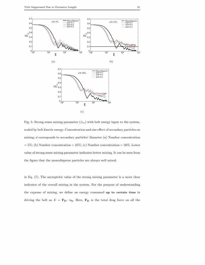
Fig. 5: Strong sense mixing parameter (βss) with belt energy input to the system,

scaled by belt kinetic energy. Concentration and size effect of secondary particles on

mixing; d corresponds to secondary particles’ diameter (a) Number concentration

= 5%; (b) Number concentration = 25%; (c) Number concentration = 50%. Lower

value of strong sense mixing parameter indicates better mixing. It can be seen from

the figure that the monodisperse particles are always well mixed.

in Eq. (7). The asymptotic value of the strong mixing parameter is a more clear

indicator of the overall mixing in the system. For the purpose of understanding

the expense of mixing, we define an energy consumed up to certain time in

driving the belt as E = FD · vb. Here, FD is the total drag force on all the


belt particles and vb is the belt velocity. Fig. 5 is a plot of βss versus the belt

energy input (E) for the bidisperse cases. It can be seen from this figure that from

an energy perspective, monodisperse systems are more efficient owing to the fact

that size segregation is not important. In addition, the kinematic motion of the

belt is transferred efficiently to all the granular material. For the other bidisperse

systems, the degree of segregation depends on the particle size variability as well

as the concentration. A higher concentration of secondary particles causes stronger

segregation while a higher diameter ratio of secondary to primary particles favours

mixing. Therefore, it appears that a low concentration of secondary particles with

their diameter being as close as possible to the mean diameter is favorable. This can

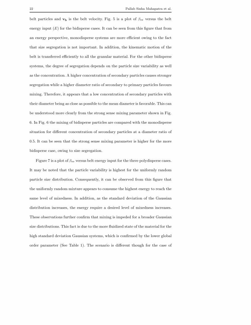
be understood more clearly from the strong sense mixing parameter shown in Fig.

6. In Fig. 6 the mixing of bidisperse particles are compared with the monodisperse

situation for different concentration of secondary particles at a diameter ratio of

0.5. It can be seen that the strong sense mixing parameter is higher for the more

bidisperse case, owing to size segregation.

Figure 7 is a plot of βss versus belt energy input for the three polydisperse cases.

It may be noted that the particle variability is highest for the uniformly random

particle size distribution. Consequently, it can be observed from this figure that

the uniformly random mixture appears to consume the highest energy to reach the

same level of mixedness. In addition, as the standard deviation of the Gaussian

distribution increases, the energy require a desired level of mixedness increases.

These observations further confirm that mixing is impeded for a broader Gaussian

size distributions. This fact is due to the more fluidized state of the material for the

high standard deviation Gaussian systems, which is confirmed by the lower global

order parameter (See Table 1). The scenario is different though for the case of


102

βss

0

0.2

0.4

0.6

0.7

0.1

0.3

0.5

105104103

E

d/D=0.5

n/N=50 %n/N=25 %n/N=5 %Monodisperse

Fig. 6: Strong sense mixing parameter (βss) with belt energy input to the system,

scaled by belt kinetic energy. Different number fraction of secondary particles

(= d/D = 0.5). The figure depicts that the lower concentration of the secondary

particles improves the mixing efficiency of the system.

uniform random distribution of particles. Firstly, the initiation of mixing marked

by the system tumbling occurs at a lower energy in these cases. In addition, for the

same time period and with the same belt velocity, this granular system consumes

lower energy than the Gaussian distribution. Remarkably, it appears to be close

to that for a monodisperse system, in spite of the wide distribution of particles.

This could be explained by the absence of any window of ‘similar’ sized particles,

unlike the Gaussian or bidisperse system for which such a window clearly exists.

Figure 8 (a) is a plot of the final value of βss versus the size ratio for

bidisperse case. For reference, the monodisperse and uniform polydisperse

values are also indicated. From the figure, it can be observed that with

an increase of the size ratio for the bi-disperse situations, βss decreases.

For any particular size ratio, βss increases with an increase of the number


102

βss

0

0.2

0.4

0.6

0.7

0.1

0.3

0.5

105104103

σ/D=0.100σ/D=0.050σ/D=0.025σ/D=0.010Monodisperse

E

(a)

102

βss

0

0.2

0.4

0.6

0.7

0.1

0.3

0.5

105104103

E

σ/D=0.1Uniform polyMonodisperse

(b)

Fig. 7: Strong sense mixing parameter (βss) with scaled belt energy. (a) Gaussian

distribution: effect of standard deviation (σ/dm);(b) Size distribution (Gaussian

with σ/dm = 10% and uniform random with dmin = 2mm and dmax = 10mm).

The figure shows that the monodisperse system exhibits highest mixing efficiency

and for the Gaussian distributed polydispersed system the mixing increases when

the standard deviation is lower. The uniformly random polydispersed system tends

to reach the monodisperse mixing efficiency.

concentration. As seen in Fig. 8(a), for higher concentration of secondary

particles the mixing efficiency decreases (higher value of βss) below that

for uniformly random mixtures. Figure 8 (b) shows the plot of the final

value of βss for Gaussian distributions with different mean particle sizes.

It can be noted that the values of βss in Fig. 8(b) are much lower than

those in Fig. 8(a) for bidisperse distributions. Figures 8(c) and (d) show

the energy required to obtain the states shown in Fig. 8(a) and (b) for

a given composition. The values of the energy for the monodisperse and

uniform polydisperse are also shown for reference. For the bidisperse cases,

better mixing is obtained at lower energy consumption with increasing size


0.00 0.02 0.04 0.06 0.08 0.100.00

0.02

0.04

0.06

0.03

0.01

0.07

0.05

σ/D

βss

0.30 0.35 0.40 0.45 0.500.00

0.02

0.04

0.06

0.08

0.10

0.12

0.14

0.16

0.18

d/D

MonodisperseUniform polydisperse

(b)

(c) (d)

(a)

n/N = 5%

n/N = 50%n/N = 25%

σ/D0.00 0.02 0.04 0.06 0.08 0.10

d/D0.30 0.35 0.40 0.45 0.50

4

4.5

5

5.5

6

6.5

7

7.5

8

E

x104

4

4.5

5

5.5

6

6.5

7

7.5

8

E

x104

βss

Fig. 8: Final value of the mixing parameter for (a) different size ratios and number

concentrations and (b) Gaussian distributions with different standard deviations

of the particle sizes. (c) The energy required to obtain the states shown in (a) for

different size ratios and (d) the energy required to obtain the state shown in (b)

for different Gaussian distribution widths.

ratios. The energy required also decreases with an increase in size ratios

and number concentration in the bidisperse case. Figure 8(d) shows the

energy required for mixing a granular material with Gaussian distribution

of particle sizes as a function of the standard deviation of the particle sizes

to achieve the states achieved in Figure 8(b). As can be seen, the energy


(b)

(c) (d)

(a)

n/N = 5%

n/N = 50%n/N = 25%

MonodisperseUniform polydisperse

βss

=0.3

d/D0.30 0.35 0.40 0.45 0.50

1

1.25

1.5

1.75

2

2.25

2.5

E

1

1.25

1.5

1.75

2

2.25

2.5

E

0.00 0.02 0.04 0.06 0.08 0.10σ/D

βss

=0.3

1

2

3

4

5

6

7

E

d/D

8

9β

ss=0.1

σ/D0.00 0.02 0.04 0.06 0.08 0.10

5

10

15

20

25

30

35

40

E

βss

=0.1

x103 x103

x104 x103

0.30 0.35 0.40 0.45 0.50

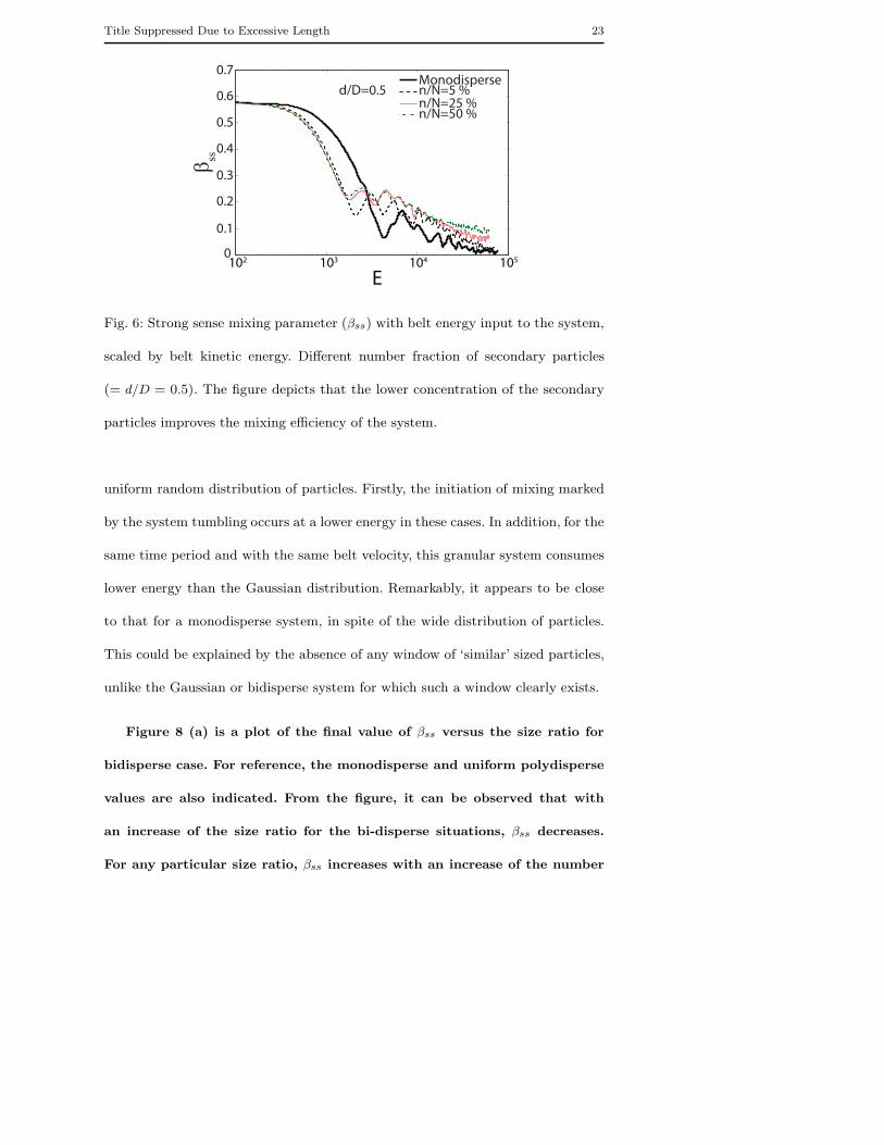
Fig. 9: Energy required for achieving a mixing parameter value of 0.3 for different

(a) size ratios and number concentrations and (b) Gaussian distribution widths.

Energy required for achieving a mixing parameter value of 0.1 for different (c) size

ratios and number concentrations and (d) Gaussian distribution widths.

required decreases with an increasing standard deviation of the particle

sizes.

Figure 9 shows the energy required for achieving βss values of 0.3 and

0.1 for bidisperse and Gaussian distributions of sizes. The energy required

to obtain βss = 0.3 is lower for increasing size ratios. It is interesting to

note that this trend is reversed and greater energy is required to obtain


βss = 0.1 as size ratio increases (see Fig. 9(c)). Figure 9(a) also indicates that

monodisperse system takes larger energy to achieve βss = 0.3 whereas, uni-

form polydisperse system takes minimum energy. Again, this trend is also

reversed in Fig. 9(c). It clearly demonstrates that initial energy requirement

to move the monodisperse particles are higher due to the inefficient transfer

of kinetic energy to the monodisperse granular system. On the other hand,

due to the segregation of particles the energy requirement is less for other

parameter conditions. To achieve more efficient mixing (βss = 0.1) the final

energy requirement for monodisperse system is lowest (as also evident from

Figs. 5, 6, 7). It should be noted that the value of βss = 0.1 has not been

achieved by certain combinations of size concentrations and number ratio

(see Fig. 9(c)). Figures 9(b) and (d) are similar to Fig. 9(a) and (c), except

that they are obtained with particle sizes following a Gaussian distribu-

tion. For all Gaussian distribution cases studied here, the energy required

to achieve βss = 0.1 is higher than the monodisperse and uniformly random

cases. It should be noted that the value of βss = 0.1 has not been achieved

by certain combinations of size concentrations and number ratio (see Fig.

9(c)).

4 Conclusion

In the present work the mixing of monodisperse and polydisperse wet granular

particles are carried out inside a belt driven enclosure. The overall mixing in a

belt-driven enclosure seems to be most efficient for a monodisperse system. In-

troducing secondary particles or size variation may lead to segregation although


it shows promising energy reduction at early stages. The advection stage mixing

is observed when segregation occurs wherupon the monodisperse system is more

energy efficient than all polydisperse systems. While segregation is prompted by a

window of similar sized particles, the study on uniformly white noise random size

distribution has revealed close similarity to the monodisperse system for overall

mixing at reduced energy costs.

Disclosures

The authors declare that they have no conflicts of interest. The computational

resources in the High Performance Cluster was provided by the Indian Institute of

Technology Madras. The data in this study was not presented earlier. No human

or animal participants have been employed in this study.

References

1. JG Benito and AM Vidales. Novel aspects on the segregation in quasi 2d piles.

Powder Technology, 234:123–131, 2013.

2. JMNT Gray and C Ancey. Multi-component particle-size segregation in shal-

low granular avalanches. Journal of Fluid Mechanics, 678:535–588, 7 2011.

3. B Remy, J G Khinast, and B J Glasser. Polydisperse granular flows in a

bladed mixer: Experiments and simulations of cohesionless spheres. Chemical

Engineering Science, 66(9):1811–1824, 2011.

4. GR Chandratilleke, AB Yu, and J Bridgwater. A dem study of the mixing

of particles induced by a flat blade. Chemical Engineering Science, 79:54–74,

2012.


5. O Dube, E Alizadeh, J Chaouki, and F Bertrand. Dynamics of non-spherical

particles in a rotating drum. Chemical Engineering Science, 101:486–502, 2013.

6. L Devriendt, C Gatumel, and H Berthiaux. Experimental evidence of mixture

segregation by particle size distribution. Particulate Science and Technology,

31(6):653–657, 2013.

7. D Nguyen, A Rasmuson, I N Bjorn, and K Thalberg. Cfd simulation of tran-

sient particle mixing in a high shear mixer. Powder Technology, 258:324–330,

2014.

8. MMHD Arntz, HH Beeftink, WK Otter, WJ Briels, and RM Boom. Segrega-

tion of granular particles by mass, radius, and density in a horizontal rotating

drum. AIChE Journal, 60(1):50–59, 2014.

9. R Collet, D Oulahna, A De Ryck, PH Jezequel, and M Martin. Mixing of a wet

granular medium: Influence of the liquid addition method. Powder Technology,

208(2):367–371, 2011.

10. A Kudrolli. Granular matter: Sticky sand. Nature materials, 7(3):174–175,

2008.

11. SS Hsiau, CC Liao, CH Tai, and CY Wang. The dynamics of wet granular

matter under a vertical vibration bed. Granular Matter, 15(4):437–446, 2013.

12. K Samiei and B Peters. Experimental and numerical investigation into the

residence time distribution of granular particles on forward and reverse acting

grates. Chemical Engineering Science, 87:234–245, 2013.

13. PY Liu, RY Yang, and AB Yu. Self-diffusion of wet particles in rotating drums.

Physics of Fluids (1994-present), 25(6):063301, 2013.

14. GG Pereira and PW Cleary. Radial segregation of multi-component granular

media in a rotating tumbler. Granular Matter, 15(6):705–724, 2013.


15. A Darelius, J Remmelgas, A Rasmuson, B van Wachem, and IN Bjrn. Fluid

dynamics simulation of the high shear mixing process. Chemical Engineering

Journal, 164(23):418 – 424, 2010. Pharmaceutical Granulation and Processing.

16. PY Liu, RY Yang, and AB Yu. Dynamics of wet particles in rotating drums:

Effect of liquid surface tension. Physics of Fluids, 23(1):013304, 2011.

17. P Kosinski, A Kosinska, and AC Hoffmann. Simulation of solid particles

behaviour in a driven cavity flow. Powder Technology, 191(3):327–339, 2009.

18. SJ Tsorng, H Capart, DC Lo, JS Lai, and DL Young. Behaviour of macroscopic

rigid spheres in lid-driven cavity flow. International Journal of Multiphase Flow,

34(1):76 – 101, 2008.

19. PD Bonkinpillewar, A Kulkarni, MV Panchagnula, and S Vedantam. A novel

coupled fluid particle dem for simulating dense granular slurry dynamics.

Granular Matter, 17(4):511–521, 2015.

20. D Rodrguez, JG Benito, I Ippolito, JP Hulin, AM Vidales, and RO Uac.

Dynamical effects in the segregation of granular mixtures in quasi 2d piles.

Powder Technology, 269:101 – 109, 2015.

21. A Misra and P Poorsolhjouy. Micro-macro scale instability in 2d regular

granular assemblies. Continuum Mechanics and Thermodynamics, 27(1-2):63–

82, 2015.

22. A Leonardi, M Cabrera, FK Wittel, R Kaitna, M Mendoza, W Wu, and

HJ Herrmann. Granular-front formation in free-surface flow of concentrated

suspensions. Phys. Rev. E, 92:052204, Nov 2015.

23. H Yin, M Zhang, and H Liu. Numerical simulation of three-dimensional un-

steady granular flows in rotary kiln. Powder Technology, 253:138–145, 2014.


24. G Juarez, IC Christov, JM Ottino, and RM Lueptow. Mixing by cutting and

shuffling 3d granular flow in spherical tumblers. Chemical Engineering Science,

73:195–207, 2012.

25. A Jain, M J Metzger, and B J Glasser. Effect of particle size distribution on

segregation in vibrated systems. Powder Technology, 237:543–553, 2013.

26. Qingqing Y, Zhiman S, Fei C, and Keizo U. Enhanced mobility of polydisperse

granular flows in a small flume. Geoenvironmental Disasters, 2(1):1–9, 2015.

27. P Jop. Rheological properties of dense granular flows. Comptes Rendus

Physique, 16(1):62–72, 2015. Granular physics / Physique des milieux granu-

laires.

28. M Latzel, S Luding, and H J Herrmann. Macroscopic material properties from

quasi-static, microscopic simulations of a two-dimensional shear-cell. Granular

Matter, 2(3):123–135, 2000.

29. C Drumm, S Tiwari, J Kuhnert, and H Bart. Finite pointset method for

simulation of the liquid–liquid flow field in an extractor. Computers & Chemical

Engineering, 32(12):2946–2957, 2008.

30. PD Bonkinpillewar, S Vedantam, and MV Panchagnula. Flow of wet granular

material in a lid driven cavity. In Seventh M.I.T. Conference on Computational

Fluid and Solid Mechanics. Massachusetts Institute of Technology, USA, June

2013.

31. WC Swope, HC Andersen, PH Berens, and KR Wilson. A computer simula-

tion method for the calculation of equilibrium constants for the formation of

physical clusters of molecules: Application to small water clusters. The Journal

of Chemical Physics, 76(1):637–649, 1982.


32. S Plimpton. Fast parallel algorithms for short-range molecular dynamics.

Journal of computational physics, 117(1):1–19, 1995.

33. J Doucet, F Bertrand, and J Chaouki. A measure of mixing from lagrangian

tracking and its application to granular and fluid flow systems. Chemical

Engineering Research and Design, 86(12):1313–1321, 2008.

34. ND Mermin. Crystalline order in two dimensions. Physical Review, 176(1):250,

1968.

35. JF Peters, M Muthuswamy, J Wibowo, and A Tordesillas. Characterization

of force chains in granular material. Physical Review E, 72:041307, 2005.

36. HM Jaeger, SR Nagel, and RP Behringer. Granular solids, liquids, and gases.

Reviews of Modern Physics, 68:1259–1273, 1996.

37. JM Ottino and DV Khakhar. Mixing and segregation of granular materials.

Annual Review of Fluid Mechanics, 32:55–91, 2000.

Documents

Eﬀect of size distribution on mixing of a polydisperse wet