Embed Size (px)
Citation preview
Chapter 6.01— Spring 2012—March 10, 2012 1
6.01 Course Notes
1 Course Overview 61.1 Goals for 6.01 61.2 Modularity, abstraction, and modeling 71.2.1 Example problem 71.2.2 An abstraction hierarchy of mechanisms 81.2.3 Models 121.3 Programming embedded systems 141.3.1 Interacting with the environment 141.3.2 Programming models 161.4 Summary 18
2 Learning to Program in Python 192.1 Using Python 192.1.1 Indentation and line breaks 202.1.2 Types and declarations 212.1.3 Modules 222.1.4 Interaction and Debugging 222.2 Procedures 232.3 Control structures 252.3.1 Conditionals 252.4 Common Errors and Messages 352.5 Python Style 362.5.1 Normalize a vector 372.5.2 Perimeter of a polygon 382.5.3 Bank transfer 382.5.4 Coding examples 39

Chapter 6.01— Spring 2012—March 10, 2012 2
3 Programs and Data 453.1 Primitives, Composition, Abstraction, and Patterns 463.2 Expressions and assignment 473.2.1 Simple expressions 473.2.2 Variables 483.3 Structured data 503.3.1 List mutation and shared structure 533.3.2 Tuples and strings 573.4 Procedures 593.4.1 Definition 593.4.2 Procedure calls 603.4.3 Non-local references 633.4.4 Environments in Python 653.4.5 Non-local references in procedures 653.4.6 Procedures as first-class objects 673.5 Object-oriented programming 723.5.1 Classes and instances 733.5.2 Methods 763.5.3 Initialization 793.5.4 Inheritance 813.5.5 Using Inheritance 843.6 Recursion 853.7 Implementing an interpreter 873.7.1 Spy 883.7.2 Evaluating Spy expressions 903.7.3 Object-Oriented Spy 983.8 Object-Oriented Programming Examples 1033.8.1 A simple method example 1033.8.2 Superclasses and inheritance 1043.8.3 A data type for times 1063.8.4 Practice problem: argmax 1083.8.5 Practice problem: OOP 1083.8.6 Practice problem: The Best and the Brightest 1093.8.7 Practice Problem: A Library with Class 112

Chapter 6.01— Spring 2012—March 10, 2012 3
4 State Machines 1154.1 Primitive state machines 1164.1.1 Examples 1174.1.2 State machines in Python 1214.1.3 Simple parking gate controller 1304.2 Basic combination and abstraction of state machines 1324.2.1 Cascade composition 1324.2.2 Parallel composition 1344.2.3 Feedback composition 1364.2.4 Plants and controllers 1444.2.5 Conditionals 1464.2.6 Switch 1464.3 Terminating state machines and sequential compositions 1494.3.1 Repeat 1504.3.2 Sequence 1514.3.3 RepeatUntil and Until 1534.4 Using a state machine to control the robot 1564.4.1 Rotate 1564.4.2 Forward 1584.4.3 Square Spiral 1584.5 Conclusion 1614.6 Examples 1624.6.1 Practice problem: Things 1624.6.2 Practice problem: Inheritance and State Machines 164
Chapter 6.01— Spring 2012—March 10, 2012 4
5 Signals and Systems 1655.1 The signals and systems abstraction 1655.1.1 Modularity, primitives, and composition 1675.1.2 Discrete-time signals and systems 1685.1.3 Linear time-invariant systems 1695.2 Discrete-time signals 1695.2.1 Unit sample signal 1705.2.2 Signal combinators 1705.2.3 Algebraic properties of operations on signals 1725.2.4 Sinusoidal primitives 1725.3 Feedforward systems 1735.3.1 Representing systems 1745.3.2 Combinations of systems 1765.4 Feedback Systems 1795.4.1 Accumulator example 1795.4.2 General form of LTI systems 1825.4.3 System functions 1825.4.4 Primitive systems 1835.4.5 Combining system functions 1845.5 Predicting system behavior 1855.5.1 First-order systems 1865.5.2 Second-order systems 1885.5.3 Higher-order systems 2005.5.4 Finding poles 2015.5.5 Superposition 2025.6 Designing systems 2035.7 Summary of system behavior 2035.8 Signals and systems in Python 2045.8.1 Signals 2045.8.2 Combined signals 2065.8.3 Transduced signals 2065.8.4 Example 2065.9 Worked Examples 2075.9.1 Specifying difference equations 2075.9.2 Difference equations and block diagrams 2085.9.3 Wall finder 2115.9.4 Cool difference equations 2165.9.5 Modeling 2175.9.6 SM to DE 2215.9.7 On the Verge 2225.9.8 What’s Cooking? 2235.9.9 Pole Position 2265.9.10 System functions 227
Chapter 6.01— Spring 2012—March 10, 2012 5
6 Circuits 2296.1 What is a circuit? 2296.1.1 Electrical circuits 2306.2 Conservation laws 2316.2.1 Kirchoff’s current law 2316.2.2 Kirchoff’s Voltage Law 2346.3 Circuit elements 2386.4 Solving circuits 2416.4.1 NVCC Method 2426.4.2 Solution strategy 2446.4.3 An example 2456.4.4 Node method (optional) 2476.4.5 Common Patterns 2496.5 Circuit Equivalents 2536.5.1 Example 2566.5.2 Norton Equivalents 2576.6 Op Amps 2576.6.1 Voltage-controlled voltage sources 2576.6.2 Simplified model 2616.6.3 Op-amps and feedback 2636.6.4 Where does the current come from? 265
Chapter 1 Course Overview 6.01— Spring 2012—March 10, 2012 6
Chapter 1Course Overview
1.1 Goals for 6.01We have many goals for this course. Our primary goal is for you to learn to appreciate and usethe fundamental design principles of modularity and abstraction in a variety of contexts fromelectrical engineering and computer science. To achieve this goal, we will study electrical engi-neering (EE) and computer science (CS) largely from the perspective of how to build systems thatinteract with, and attempt to control, an external environment. Such systems include everythingfrom low-level controllers like heat regulators or cardiac pacemakers, tomedium-level systems likeautomated navigation or virtual surgery, to high-level systems that provide more natural human-computer interfaces.
Our second goal is to show you that making mathematical models of real systems can help in thedesign and analysis of those systems; and to give you practice with the difficult step of decidingwhich aspects of the real world are important to the problem being solved and how tomodel themin ways that give insight into the problem.
We also hope to engage you more actively in the educational process. Most of the work of thiscourse will not be like typical problems from the end of a chapter. You will work individually andin pairs to solve problems that are deeper and more open-ended. There will not be a unique rightanswer. Argument, explanation, and justification of approach will be more important than theanswer. We hope to expose you to the ubiquity of trade-offs in engineering design: it is rare thatan approach will be best in every dimension; some will excel in one way, others in a different way.Deciding how to make such trade-offs is a crucial part of engineering.
Another way in which we hope to engage you in the material is by having many of you returnto the course as lab assistants in future semesters. Having a large number of lab assistants in theclass means that students can be given more open-ended problems, and have people around tohelp them when they are stuck. Even more importantly, the lab assistants are meant to questionthe students as they go; to challenge their understanding and help them see and evaluate a varietyof approaches. This process is of great intellectual value to student and lab assistant alike.
Finally, of course, we have the more typical goals of teaching exciting and important basic ma-terial from electrical engineering and computer science, including modern software engineering,linear systems analysis, electronic circuits, and decision-making. This material all has an internalelegance and beauty, and plays a crucial role in building modern EE and CS systems.

Chapter 1 Course Overview 6.01— Spring 2012—March 10, 2012 7
1.2 Modularity, abstraction, and modelingWhether proving a theorem by building up from lemmas to basic theorems to more specializedresults, or designing a circuit by building up from components to modules to complex processors,or designing a software system by building up from generic procedures to classes to class libraries,humans deal with complexity by exploiting the power of abstraction and modularity. Withoutsuch tools, a single person would be overwhelmed by the complexity of a system, as there is onlyso much detail that a single person can consciously manage at a time.
Modularity is the idea of building components that can be re-used; and abstraction is the idea thatafter constructing a module (be it software or circuits or gears), most of the details of the moduleconstruction can be ignored and a simpler description used for module interaction (the modulecomputes the square root, or doubles the voltage, or changes the direction of motion).
Given basic modules, one can move up a level of abstraction and construct a new module byputting together several previously-built modules, thinking only of their abstract descriptions,and not their implementations. And, of course, this process can be repeated over many stages.This process gives one the ability to construct systems with complexity far beyond what would bepossible if it were necessary to understand each component in detail.
Any module can be described in a large number of ways. We might describe the circuitry in adigital watch in terms of how it behaves as a clock and a stopwatch, or in terms of voltages andcurrents within the circuit, or in terms of the heat produced at different parts of the circuitry. Eachof these is a different model of the watch. Different models will be appropriate for different tasks:there is no single correct model. Rather, each model exposes different dimensions of the system,allowing us to explore many aspects of the design space of a system, and to trade off differentfactors in the performance of a system.
The primary theme of this course will be to learn about different methods for building modulesout of primitives, and of building different abstract models of them, so that we can analyze orpredict their behavior, and so we can recombine them into even more complex systems. The samefundamental principles will apply to software, to control systems, and to circuits.
1.2.1 Example problemImagine that you need to make a robot that will roll up close to a light bulb and stop a fixeddistance from it. The first question is, how can we get electrical signals to relate to the physicalphenomena of light readings and robot wheel rotations? There is a large part of electrical engi-neering related to the design of physical devices that connect to the physical world in such a waythat some electrical property of the device relates to a physical process in the world. For example,a light-sensitive resistor (photo-resistor) is a sensor whose resistance changes depending on lightintensity impinging on it; a motor is an effector whose rotor speed is related to the voltage acrossits two terminals. In this course, we will not examine the detailed physics of sensors and effectors,but will concentrate on ways of designing systems that use sensors and effectors to perform bothsimple and more complicated tasks. To get a robot to stop in front of a light bulb, the problemwillbe to find a way to connect the photo-resistor to the motor, so that the robot will stop at an appro-priate distance from the bulb. Thus, we will already use the idea of abstraction to treat sensorsand effectors as primitive modules whose internal details we can ignore, and whose performancecharacteristics we can use as we design systems built on these elements.

Chapter 1 Course Overview 6.01— Spring 2012—March 10, 2012 8
1.2.2 An abstraction hierarchy of mechanismsGiven the light-sensitive resistor and the motor, we could find many ways of connecting them,using bits of metal and ceramic of different kinds, or making some kind of magnetic or mechanicallinkages. The space of possible designs of machines is enormous.
One of themost important things that engineers do, when facedwith a set of design problems, is tostandardize on a basis set of components to use to build their systems. There are many reasons forstandardizing on a basis set of components, mostly having to do with efficiency of understandingand of manufacturing. It is important, as a designer, to develop a repertoire of standard bits andpieces of designs that you understand well and can put together in various ways to make morecomplex systems. If you use the same basis set of components as other designers, you can learnvaluable techniques from them, rather than having to re-invent the techniques yourself. And otherpeople will be able to readily understand and modify your designs.
We can often make a design job easier by limiting the space of possible designs, and by standard-izing on:• a basis set of primitive components;• ways of combining the primitive components to make more complex systems;• ways of “packaging” or abstracting pieces of a design so they can be reused (in essence creating
new “primitives”); and• ways of capturing common patterns of abstraction (essentially, abstracting our abstractions).
Very complicated design problems can become tractable using such a primitive-combination-abstraction-pattern (PCAP) approach. In this class, we will examine and learn to use a varietyof PCAP strategies common in EE and CS, and will even design some of our own, for specialpurposes. In the rest of this section, we will hint at some of the PCAP systems we will bedeveloping in much greater depth throughout the class. Figure 1.1 shows one view of thisdevelopment, as a successive set of restrictions of the design space of mechanisms.
electrical systems
traditional analog circuits
digital electronic circuits
electronic computers
electronic computers running Python programs
electronic computers with Python programs that
select outputs by planning
Figure 1.1 Increasingly constrained systems.
One very important thing about abstract models is that once we have fixed the abstraction, it willusually be possible to implement it using a variety of different underlying substrates. So, as shown
Chapter 1 Course Overview 6.01— Spring 2012—March 10, 2012 9
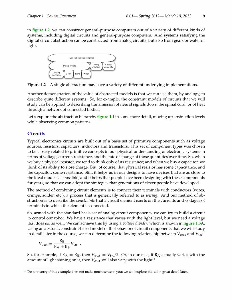
in figure 1.2, we can construct general-purpose computers out of a variety of different kinds ofsystems, including digital circuits and general-purpose computers. And systems satisfying thedigital circuit abstraction can be constructed from analog circuits, but also from gears or water orlight.
General-purpose computer
Digital circuits Turing machine
Cellular automata
Analog electronics Gears Light Water
Figure 1.2 A single abstraction may have a variety of different underlying implementations.
Another demonstration of the value of abstracted models is that we can use them, by analogy, todescribe quite different systems. So, for example, the constraint models of circuits that we willstudy can be applied to describing transmission of neural signals down the spinal cord, or of heatthrough a network of connected bodies.
Let’s explore the abstraction hierarchy figure 1.1 in somemore detail, moving up abstraction levelswhile observing common patterns.
CircuitsTypical electronics circuits are built out of a basis set of primitive components such as voltagesources, resistors, capacitors, inductors and transistors. This set of component types was chosento be closely related to primitive concepts in our physical understanding of electronic systems interms of voltage, current, resistance, and the rate of change of those quantities over time. So, whenwe buy a physical resistor, we tend to think only of its resistance; and when we buy a capacitor, wethink of its ability to store charge. But, of course, that physical resistor has some capacitance, andthe capacitor, some resistance. Still, it helps us in our designs to have devices that are as close tothe ideal models as possible; and it helps that people have been designing with these componentsfor years, so that we can adopt the strategies that generations of clever people have developed.
The method of combining circuit elements is to connect their terminals with conductors (wires,crimps, solder, etc.), a process that is generically referred to as wiring. And our method of ab-straction is to describe the constraints that a circuit element exerts on the currents and voltages ofterminals to which the element is connected.
So, armed with the standard basis set of analog circuit components, we can try to build a circuitto control our robot. We have a resistance that varies with the light level, but we need a voltagethat does so, as well. We can achieve this by using a voltage divider, which is shown in figure 1.3A.Using an abstract, constraint-basedmodel of the behavior of circuit components that wewill studyin detail later in the course, we can determine the following relationship between Vout and Vin:
Vout =RB
RA + RBVin .
So, for example, if RA = RB, then Vout = Vin/2. Or, in our case, if RA actually varies with theamount of light shining on it, then Vout will also vary with the light.1
Do not worry if this example does not make much sense to you; we will explore this all in great detail later.1

Chapter 1 Course Overview 6.01— Spring 2012—March 10, 2012 10Chapter 1 Course Overview 6.01— Spring 2011— April 9, 2011 10
RA
RB
Vin
Vout
RA
RB
Vin
Vout
motor
RA
RB
Vin
Vout
motor
Figure 1.3 Voltage dividers: A. Resistor divider. B. Connected to a motor, in a way that breaks theabstraction from part A. C. Connected to a motor, with a buffer.
That is great. So, now, we might imagine that we could use this voltage difference that we havecreated to drive the motor at different speeds, depending on the light hitting the resistor, using acircuit something like the one shown in figure 1.3B. But, sadly, that will not work. It turns out thatonce we connect the motor to the circuit, it actually changes the voltages, and we can no longermaintain the voltage difference needed to drive the motor.
So, although we have developed an abstract model of the behavior of circuit components, whichlets us analyze the behavior of a particular complete circuit design, it does not give us modular-ity. That is, we cannot design two parts of a circuit, understand each of their behaviors, and thenpredict the behavior of the composite system based on the behavior of the separate components.Instead, we would have to re-analyze the joint behavior of the whole composite system. Lack ofmodularity makes it very difficult to design large systems, because two different people, or thesame person at two different times, cannot design pieces and put them together without under-standing the whole.
To solve this problem, we can augment our analog-circuit toolbox with some additional compo-nents that allow us to design components with modular behavior; they “buffer” or “isolate” onepart of the circuit from another in ways that allow us to combine the parts more easily. In thisclass, we will use op-amps to build buffers, which will let us solve our sample problem using aslightly more complex circuit, as shown in figure 1.3C.
Thus, the key point is that good modules preserve abstraction barriers between the use of a mod-ule and internal details of how they are constructed. We will see this theme recur as we discussdifferent PCAP systems.
Digital circuitsIn analog circuits, we think about voltages on terminals ranging over real values. This gives usthe freedom to create an enormous variety of circuits, but sometimes that freedom actually makesthe design process more difficult. To design ever more complex circuits, we can move to a muchstronger, digital abstraction, in which the voltages on the terminals are thought of as only takingon values that are either “low” or “high” (often called 0 and 1). This PCAP system is made upof a basis set of elements, called gates, that are built out of simpler analog circuit components,such as transistors and resistors. Adopting the digital abstraction is a huge limitation on the kindsof circuits that can be built. However, digital circuits can be easy to design and build and also
Figure 1.3 Voltage dividers: A. Resistor divider. B. Connected to a motor, in a way that breaks theabstraction from part A. C. Connected to a motor, with a buffer.
That is great. So, now, we might imagine that we could use this voltage difference that we havecreated to drive the motor at different speeds, depending on the light hitting the resistor, using acircuit something like the one shown in figure 1.3B. But, sadly, that will not work. It turns out thatonce we connect the motor to the circuit, it actually changes the voltages, and we can no longermaintain the voltage difference needed to drive the motor.
So, although we have developed an abstract model of the behavior of circuit components, whichlets us analyze the behavior of a particular complete circuit design, it does not give us modular-ity. That is, we cannot design two parts of a circuit, understand each of their behaviors, and thenpredict the behavior of the composite system based on the behavior of the separate components.Instead, we would have to re-analyze the joint behavior of the whole composite system. Lack ofmodularity makes it very difficult to design large systems, because two different people, or thesame person at two different times, cannot design pieces and put them together without under-standing the whole.
To solve this problem, we can augment our analog-circuit toolbox with some additional compo-nents that allow us to design components with modular behavior; they “buffer” or “isolate” onepart of the circuit from another in ways that allow us to combine the parts more easily. In thisclass, we will use op-amps to build buffers, which will let us solve our sample problem using aslightly more complex circuit, as shown in figure 1.3C.
Thus, the key point is that good modules preserve abstraction barriers between the use of a mod-ule and internal details of how they are constructed. We will see this theme recur as we discussdifferent PCAP systems.
Digital circuitsIn analog circuits, we think about voltages on terminals ranging over real values. This gives usthe freedom to create an enormous variety of circuits, but sometimes that freedom actually makesthe design process more difficult. To design ever more complex circuits, we can move to a muchstronger, digital abstraction, in which the voltages on the terminals are thought of as only takingon values that are either “low” or “high” (often called 0 and 1). This PCAP system is made upof a basis set of elements, called gates, that are built out of simpler analog circuit components,such as transistors and resistors. Adopting the digital abstraction is a huge limitation on the kindsof circuits that can be built. However, digital circuits can be easy to design and build and alsocan be inexpensive because the basic elements (gates) are simple (fewer transisters are need toconstruct a gate than to construct an op amp), versatile (only a small number of different kindsof logic elements are necessary to construct an arbitrary digital circuit), and combinations areeasy to think about (using Boolean logic). These properties allow designers to build incredibly
Chapter 1 Course Overview 6.01— Spring 2012—March 10, 2012 11
complex machines by designing small parts and putting them together into increasingly largerpieces. Digital watches, calculators, and computers are all built this way.
Digital design is a very important part of EECS, and it is treated in a number of our courses at basicand advanced levels, but is not one of the topics we will go into in detail in 6.01. Nevertheless, thesame central points that we explore in this course apply to this domain as well.
ComputersOne of the most important developments in the design of digital circuits is that of the general-purpose “stored program” computer. Computers are a particular class of digital circuits that aregeneral purpose: the same actual circuit can perform (almost) any transformation between its in-puts and its outputs. Which particular transformation it performs is governed by aprogram,whichis some settings of physical switches, or informationwritten on an external physical memory, suchas cards or a tape, or information stored in some sort of internal memory.
The “almost” in the previous section refers to the actual memory capacity of the computer. Ex-actly what computations a computer can perform depends on the amount of memory it has; andalso on the time you are willing to wait. So, although a general-purpose computer can do any-thing a special-purpose digital circuit can do, in the information-processing sense, the computermight be slower or use more power. However, using general-purpose computers can save an enor-mous amount of engineering time and effort. It is much cheaper and easier to debug and modifyand manufacture software than hardware. The modularities and abstractions that software PCAPsystems give us are even more powerful than those derived from the digital circuit abstraction.
Again, we can see how abstraction separates use from details; we don’t need to know how thecircuits inside a computer are designed, we just need to know the rules by which we can use themand the constraints under which they perform.
Python programsEvery general-purpose computer has a different detailed design, which means that the way itsprogram needs to be specified is different. Furthermore, the “machine languages” for describingcomputer programs, at the most primitive level, are awkward for human programmers. So, wehave developed a number of computer programming languages for specifying a desired computa-tion. These languages are converted into instructions in the computer’s native machine languageby other computer programs, called compilers or interpreters. One of the coolest and most powerfulthings about general-purpose computers is this ability to write computer programs that processor create or modify other computer programs.
Computer programming languages are PCAP systems. They provide primitive operations, waysof combining them, ways of abstracting over them, and ways of capturing common abstractionpatterns. We will spend a considerable amount of time in this course studying the particularprimitives, combination mechanisms, and abstraction mechanisms made available in the Pythonprogramming language. But the choice of Python is relatively unimportant. Virtually all mod-ern programming languages supply a similar set of mechanisms, and the choice of programminglanguage is primarily a matter of taste and convenience.
In a computer program we have both data primitives and computation primitives. At the mostbasic level, computers generally store binary digits (bits) in groups of 32 or 64, called words. Thesewords are data primitives, and they can be interpreted by our programs as representing integers,
Chapter 1 Course Overview 6.01— Spring 2012—March 10, 2012 12
floating-point numbers, strings, or addresses of other data in the computer’smemory. The compu-tational primitives supported by most computers include numerical operations such as additionand multiplication, and locating and extracting the contents of a memory at a given address. InPython, we will work at a level of abstraction that does not require us to think very much aboutaddresses of data, but it is useful to understand that level of description, as well.
Primitive data and computation elements can be combined and abstracted in a variety of differ-ent ways, depending on choices of programming style. We will explore these in more detail insection 1.3.2.
1.2.3 ModelsSo far, we have discussed a number of ways of framing the problem of designing and constructingmechanisms. Each PCAP system is accompanied by a modeling system that lets us make mathe-matical models of the systems we construct.
What is a model? It is a new system that is considerably simpler than the system being modeled,but which captures the important aspects of the original system. Wemight make a physical modelof an airplane to test in a wind tunnel. It does not have to have passenger seats or landing lights;but it has to have surfaces of the correct shape, in order to capture the important properties forthis purpose. Mathematical models can capture properties of systems that are important to us,and allow us to discover things about the system much more conveniently than by manipulatingthe original system itself.
One of the hardest things about building models is deciding which aspects of the original systemto model and which ones to ignore. Many classic, dramatic engineering failures can be ascribed tofailing to model important aspects of the system. One example (which turned out to be an ethicalsuccess story, rather than a failure) is LeMessurier’s Citicorp Building2, in which an engineeringdesign change was made, but tested in a model in which the wind came only from a limited set ofdirections.
Another important dimension inmodeling iswhether themodel is deterministic or not. Wemight,for example, model the effect of the robot executing a command to set its velocity as making aninstantaneous change to the commanded velocity. But, of course, there is likely to be some delayand some error. We have to decide whether to ignore that delay and error in our model and treatit as if it were ideal; or, for example, to make a probabilistic model of the possible results of thatcommand. Generally speaking, the more different the possible outcomes of a particular actionor command, and the more diffuse the probability distribution over those outcomes, the moreimportant it is to explicitly include uncertainty in the model.
Once we have a model, we can use it in a variety of different ways, which we explore below.
Analytical modelsBy far the most prevalent use of models is in analysis: Given a circuit design, what will the voltageon this terminal be? Given a computer program, will it compute the desired answer? How longwill it take? Given a control system, implemented as a circuit or as a program, will the system stopat the right distance from the light bulb?
See “The Fifty-Nine Story Crisis”, The New Yorker, May 29, 1995, pp 45-53.2
Chapter 1 Course Overview 6.01— Spring 2012—March 10, 2012 13
Analytical tools are important. It can be hard to verify the correctness of a system by trying it in allpossible initial conditionswith all possible inputs; sometimes it is easier to develop amathematicalmodel and then prove a theorem about the model.
For some systems, such as pure software computations, or the addition circuitry in a calculator,it is possible to analyze correctness or speed with just a model of the system in question. Forother systems, such as fuel injectors, it is impossible to analyze the correctness of the controllerwithout also modeling the environment (or “plant”) to which it is connected, and then analyzingthe behavior of the coupled system of the controller and environment.
To demonstrate some of these tradeoffs, we can do a very simple analysis of a robotmoving towarda lamp. Imagine that we arrange it so that the robot’s velocity at time t, V[t], is proportional to thedifference between the actual light level, X[t], and a desired light level (that is, the light level weexpect to encounter when the robot is the desired distance from the lamp), Xdesired; that is, wecan model our control system with the difference equation
V[t] = k(Xdesired − X[t])
where k is the constant of proportionality, or gain, of the controller.Now, we need to model the world. For simplicity, we equate the light level to the robot’s position(assuming that the units match); in addition we assume the robot’s position at time t is its positionat time t− 1 plus its velocity at time t− 1 (actually, this should be the product of the velocity andthe length of time between samples, but we can just assume a unit time step and thus use velocity).When we couple these models, we get the difference equation
X[t] = X[t− 1] + k(Xdesired − X[t− 1]) .
Now, for a given value of k, we can determine how the system will behave over time, by solvingthe difference equation in X.
Later in the course, we will see how easily-determined mathematical properties of a difference-equationmodel can tell uswhether a control systemwill have the desired behavior andwhether ornot the controller will cause the system to oscillate. These same kinds of analyses can be appliedto robot control systems as well as to the temporal properties of voltages in a circuit, and evento problems as unrelated as the consequences of a monetary policy decision in economics. It isimportant to note that treating the system as moving in discrete time steps is an approximationto underlying continuous dynamics; it can make models that are easier to analyze, but it requiressophisticated understanding of sampling to understand the effects of this approximation on thecorrectness of the results.
Synthetic modelsOne goal of many people in a variety of sub-disciplines of computer science and electrical engi-neering is automatic synthesis of systems from formal descriptions of their desired behavior. Forexample, you might describe some properties you would want the input/output behavior of a cir-cuit or computer program to have, and then have a computer system discover a circuit or programwith the desired property.
This is a well-specified problem, but generally the search space of possible circuits or programsis much too large for an automated process; the intuition and previous experience of an experthuman designer cannot yet be matched by computational search methods.

Chapter 1 Course Overview 6.01— Spring 2012—March 10, 2012 14
However, humans use informal models of systems for synthesis. The documentation of a softwarelibrary, which describes the function of the various procedures, serves as an informal model thata programmer can use to assemble those components to build new, complex systems.
Internal modelsAs we wish to build more and more complex systems with software programs as controllers, wefind that it is often useful to build additional layers of abstraction on top of the one provided by ageneric programming language. This is particularly truewhen the nature of the exact computationrequired depends considerably on information that is only received during the execution of thesystem.
Consider, for example, an automated taxi robot (or, more prosaically, the navigation system inyour new car). It takes, as input, a current location in the city and a goal location, and gives, asoutput, a path from the current location to the goal. It has a map built into it.
It is theoretically possible to build an enormous digital circuit or computer program that containsa look-up table, in which we precompute the path for all pairs of locations and store them away.Thenwhenwewant to find a path, we could simply look in the table at the location correspondingto the start and goal location and retrieve the precomputed path. Unfortunately, the size of thattable is too huge to contemplate. Instead, what we do is construct an abstraction of the problemas one of finding a path from any start state to any goal state, through a graph (an abstract math-ematical construct of “nodes” with “arcs” connecting them). We can develop and implement ageneral-purpose algorithm that will solve any shortest-path problem in a graph. That algorithmand implementation will be useful for a wide variety of possible problems. And for the navigationsystem, all we have to do is represent the map as a graph, specify the start and goal states, and callthe general graph-search algorithm.
We can think of this process as actually putting amodel of the system’s interactionswith theworldinside the controller; it can consider different courses of action in the world and pick the one thatis the best according to some criterion.
Another example of using internal models is when the system has some significant lack of infor-mation about the state of the environment. In such situations, it may be appropriate to explicitlymodel the set of possible states of the external world and their associated probabilities, and toupdate this model over time as new evidence is gathered. We will pursue an example of thisapproach near the end of the course.
1.3 Programming embedded systemsThere are many different ways of thinking about modularity and abstraction for software. Differ-ent models will make some things easier to say and do and others more difficult, making differentmodels appropriate for different tasks. In the following sections, we explore different strategies forbuilding software systems that interact with an external environment, and then different strategiesfor specifying the purely computational part of a system.
1.3.1 Interacting with the environmentIncreasingly, computer systems need to interact with the world around them, receiving informa-tion about the external world, and taking actions to affect the world. Furthermore, the world is

Chapter 1 Course Overview 6.01— Spring 2012—March 10, 2012 15
dynamic, so that as the system is computing, the world is changing, requiring future computationto adapt to the new state of the world.
There are a variety of different ways to organize computations that interact with an external world.Generally speaking, such a computation needs to:1. get information from sensors (light sensors, sonars, mouse, keyboard, etc.),2. perform computation, remembering some of the results, and3. take actions to change the outside world (move the robot, print, draw, etc.).
These operations can be put together in different styles.
1.3.1.1 SequentialThe most immediately straightforward style for constructing a program that interacts with theworld is the basic imperative style, in which the program gives a sequence of ’commands’ to thesystem it is controlling. A library of special procedures is defined, some ofwhich read informationfrom the sensors and others of which cause actions to be performed. Example procedures mightmove a robot forward a fixed distance, or send a file out over the network, or move video-gamecharacters on the screen.
In this model, we could naturally write a program that moves an idealized robot in a square, ifthere is space in front of it.
if noObstacleInFront:moveDistance(1)turnAngle(90)moveDistance(1)turnAngle(90)moveDistance(1)turnAngle(90)moveDistance(1)turnAngle(90)
The major problem with this style of programming is that the programmer has to remember tocheck the sensors sufficiently frequently. For instance, if the robot checks for free space in front,and then starts moving, it might turn out that a subsequent sensor reading will show that thereis something in front of the robot, either because someone walked in front of it or because theprevious reading was erroneous. It is hard to have the discipline, as a programmer, to rememberto keep checking the sensor conditions frequently enough, and the resulting programs can be quitedifficult to read and understand.
For the robot moving toward the light, we might write a program like this:
while lightValue < desiredValue:moveDistance(0.1)
This would have the robot creep up, step by step, toward the light. We might want to modify it sothat the robot moved a distance that was related to the difference between the current and desiredlight values. However, if it takes larger steps, then during the time that it is moving it will not besensitive to possible changes in the light value and cannot react immediately to them.

Chapter 1 Course Overview 6.01— Spring 2012—March 10, 2012 16
1.3.1.2 Event-DrivenUser-interface programs are often best organized differently, as event-driven (also called interruptdriven) programs. In this case, the program is specified as a collection of procedures (called ’han-dlers’ or ’callbacks’) that are attached to particular events that can take place. So, for example,there might be procedures that are called when the mouse is clicked on each button in the inter-face, when the user types into a text field, or when the temperature of a reactor gets too high. An“event loop” runs continuously, checking to see whether any of the triggering events have hap-pened, and, if they have, calling the associated procedure.
In our simple example, we might imagine writing a program that told the robot to drive forwardby default; and then install an event handler that says that if the light level reaches the desiredvalue, it should stop. This program would be reactive to sudden changes in the environment.
As the number and frequency of the conditions that need responses increases, it can be difficult toboth keep a program like this running well and guarantee a minimum response time to any event.
1.3.1.3 TransducerAn alternative view is that programming a system that interacts with an external world is likebuilding a transducer with internal state. Think of a transducer as a processing box that runs con-tinuously. At regular intervals (perhaps many times per second), the transducer reads all of thesensors, does a small amount of computation, stores some values it will need for the next compu-tation, and then generates output values for the actions.
This computation happens over and over and over again. Complex behavior can arise out of thetemporal pattern of inputs and outputs. So, for example, a robot might try to move forward with-out hitting something by defining a procedure:
def step():distToFront = min(frontSonarReadings)motorOutput(gain * (distToFront - desiredDistance), 0.0)
Executed repeatedly, this program will automatically modulate the robot’s speed to be propor-tional to the free space in front of it.
The main problem with the transducer approach is that it can be difficult to do tasks that arefundamentally sequential (like the example of driving in a square, shown above). We will startwith the transducer model, and then, as described in section 4.3, we will build a new abstractionlayer on top of it that will make it easy to do sequential commands, as well.
1.3.2 Programming modelsJust as there are different strategies for organizing entire software systems, there are differentstrategies for formally expressing computational processes within those structures.
1.3.2.1 Imperative computationMost of you have probably been exposed to an imperative model of computer programming, inwhich we think of programs as giving a sequential set of instructions to the computer to do some-thing. And, in fact, that is how the internals of the processors of computers are typically structured.
Chapter 1 Course Overview 6.01— Spring 2012—March 10, 2012 17
So, in Java or C or C++, you write typically procedures that consist of lists of instructions to thecomputer:1. Put this value in this variable2. Square the variable3. Divide it by pi4. If the result is greater than 1, return the result
In this model of computation, the primitive computational elements are basic arithmetic opera-tions and assignment statements. We can combine the elements using sequences of statements,and control structures such as if, for, and while. We can abstract away from the details of acomputation by defining a procedure that does it. Now, the engineer only needs to know thespecifications of the procedure, but not the implementation details, in order to use it.
1.3.2.2 Functional computationAnother style of programming is the functional style. In this model, we gain power through func-tion calls. Rather than telling the computer to do things, we ask it questions: What is 4 + 5? Whatis the square root of 6? What is the largest element of the list?
These questions can all be expressed as asking for the value of a function applied to some argu-ments. But where do the functions come from? The answer is, from other functions. We start withsome set of basic functions (like “plus”), and use them to construct more complex functions.
This method would not be powerful without the mechanisms of conditional evaluation and recur-sion. Conditional functions ask one question under some conditions and another question underother conditions. Recursion is a mechanism that lets the definition of a function refer to the func-tion being defined. Recursion is as powerful as iteration.
In this model of computation, the primitive computational elements are typically basic arithmeticand list operations. We combine elements using function composition (using the output of onefunction as the input to another), if, and recursion. We use function definition as a method ofabstraction, and the idea of higher-order functions (passing functions as arguments to other func-tions) as a way of capturing common high-level patterns.
1.3.2.3 Data structuresIn either style of asking the computer to do work for us, we have another kind of modularity andabstraction, which is centered around the organization of data.
At the most primitive level, computers operate on collections of (usually 32 or 64) bits. We can in-terpret such a collection of bits as representing different things: a positive integer, a signed integer,a floating-point number, a Boolean value (true or false), one or more characters, or an address ofsome other data in the memory of the computer. Python gives us the ability to work directly withall of these primitives, except for addresses.
There is only so much you can do with a single number, though. We would like to build computerprograms that operate on representations of documents or maps or circuits or social networks. Todo so, we need to aggregate primitive data elements into more complex data structures. These caninclude lists, arrays, dictionaries, and other structures of our own devising.
Chapter 1 Course Overview 6.01— Spring 2012—March 10, 2012 18
Here, again, we gain the power of abstraction. We canwrite programs that do operations on a datastructure representing a social network, for example, without having to worry about the details ofhow the social network is represented in terms of bits in the machine.
1.3.2.4 Object-oriented programming: computation + data structuresObject-oriented programming is a style that applies the ideas of modularity and abstraction toexecution and data at the same time.
An object is a data structure, together with a set of procedures that operate on the data. Basicprocedures can be written in an imperative or a functional style, but ultimately there is imperativeassignment to state variables in the object.
One major new type of abstraction in OO programming is “generic” programming. It might bethat all objects have a procedure called print associated with them. So, we can ask any object toprint itself, without having to know how it is implemented. Or, in a graphics system, we mighthave a variety of different objects that know their x, y positions on the screen. So each of them canbe asked, in the same way, to say what their position is, even though they might be representedvery differently inside the objects.
In addition, most object-oriented systems support inheritance, which is a way to make new kindsof objects by saying that they are mostly like another kind of object, but with some exceptions.This is another way to take advantage of abstraction.
Programming languagesPython as well as other modern programming languages, such as Java, Ruby and C++, supportall of these programming models. The programmer needs to choose which programming modelbest suits the task. This is an issue that we will return to throughout the course.
1.4 SummaryWe hope that this course will give you a rich set of conceptual tools and practical techniques, aswell as an appreciation of how math, modeling, and implementation can work together to enablethe design and analysis of complex computational systems that interact with the world.
AcknowledgmentsThanks to JacobWhite, Hal Abelson, Tomas Lozano-Perez, Sarah Finney, Sari Canelake, Eric Grim-son, Ike Chuang, and Berthold Horn for useful comments and criticisms, and to Denny Freemanfor significant parts and most of the figures in the linear systems chapter. - LPK
Chapter 2 Learning to Program in Python 6.01— Spring 2012—March 10, 2012 19
Chapter 2Learning to Program in Python
Depending on your previous programming background, we recommend different paths throughthe available readings:• If you have never programmed before: you should start with a general introduction to pro-
gramming and Python. We recommendPython for Software Design: How to Think Like a ComputerScientist, by Allen Downey. This is a good introductory text that uses Python to present basicideas of computer science and programming. It is available for purchase in hardcopy, or as afree download from:
http://www.greenteapress.com/thinkpython
After that, you can go straight to the next chapter.• If you have programmed before, but not in Python: you should read the rest of this chapter
for a quick overview of Python, and how itmay differ from other programming languageswithwhich you are familiar.
• If you have programmed in Python: you should skip to the next chapter.
Everyone should have a bookmark in their browser for Python Tutorial, by Guido Van Rossum. Thisis the standard tutorial reference by the inventor of Python. It is accessible at:
http://docs.python.org/tut/tut.html
In the rest of this chapter, we will assume you know how to program in some language, but arenew to Python. We will use Java as an informal running comparative example. In this section wewill cover what we think are the most important differences between Python and what you mayalready know about programming; but these notes are by no means complete.
2.1 Using PythonPython is designed for easy interaction between a user and the computer. It comes with an in-teractive mode called a listener or shell. The shell gives a prompt (usually something like »>) andwaits for you to type in a Python expression or program. Then it will evaluate the expression youentered, and print out the value of the result. So, for example, an interaction with the Python shellmight look like this:
>>> 5 + 510>>> x = 6>>> x6

Chapter 2 Learning to Program in Python 6.01— Spring 2012—March 10, 2012 20
>>> x + x12>>> y = ’hi’>>> y + y’hihi’>>>
So, you can use Python as a fancy calculator. And as you define your own procedures in Python,you can use the shell to test them or use them to compute useful results.
2.1.1 Indentation and line breaksEvery programming language has to have some method for indicating grouping of instructions.Here is how you write an if-then-else structure in Java:
if (s == 1)s = s + 1;a = a - 10;
else s = s + 10;a = a + 10;
The braces specify what statements are executed in the if case. It is considered good style toindent your code to agree with the brace structure, but it is not required. In addition, the semi-colons are used to indicate the end of a statement, independent of the locations of the line breaksin the file. So, the following code fragment has the same meaning as the previous one, althoughit is much harder to read and understand.
if (s == 1)s = s+ 1; a = a - 10;
else s = s + 10;
a = a + 10;
In Python, on the other hand, there are no braces for grouping or semicolons for termination.Indentation indicates grouping and line breaks indicate statement termination. So, in Python, wewould write the previous example as
if s == 1:s = s + 1a = a - 10
else:s = s + 10a = a + 10
There is no way to put more than one statement on a single line.3 If you have a statement that istoo long for a line, you can signal it with a backslash:
Actually, you can write something like if a > b: a = a + 1 all on one line, if the work you need to do inside an3
if or a for is only one line long.
Chapter 2 Learning to Program in Python 6.01— Spring 2012—March 10, 2012 21
aReallyLongVariableNameThatMakesMyLinesLong = \aReallyLongVariableNameThatMakesMyLinesLong + 1
It is easy for Java programmers to get confused about colons and semi-colons in Python. Here isthe deal: (1) Python does not use semi-colons; (2) Colons are used to start an indented block, sothey appear on the first line of a procedure definition, when starting a while or for loop, andafter the condition in an if, elif, or else.
Is one method better than the other? No. It is entirely a matter of taste. The Python method ispretty unusual. But if you are going to use Python, you need to remember that indentation andline breaks are significant.
2.1.2 Types and declarationsJava programs are what is known as statically and strongly typed. Thus, the types of all the variablesmust be known at the time that the program is written. This means that variables have to bedeclared to have a particular type before they are used. It also means that the variables cannot beused in a way that is inconsistent with their type. So, for instance, you would declare x to be aninteger by saying
int x;x = 6 * 7;
But you would get into trouble if you left out the declaration, or did
int x;x = "thing";
because a type checker is run on your program to make sure that you don’t try to use a variable ina way that is inconsistent with its declaration.
In Python, however, things are a lotmore flexible. There are no variable declarations, and the samevariable can be used at different points in your program to hold data objects of different types. So,the following is fine, in Python:
if x == 1:x = 89.3
else:x = "thing"
The advantage of having type declarations and compile-time type checking, as in Java, is that acompiler can generate an executable version of your program that runs very quickly, because itcan be certain about what kind of data is stored in each variable, and it does not have to check it atruntime. An additional advantage is that many programming mistakes can be caught at compiletime, rather than waiting until the program is being run. Java would complain even before yourprogram started to run that it could not evaluate
3 + "hi"
Python would not complain until it was running the program and got to that point.
The advantage of the Python approach is that programs are shorter and cleaner looking, and pos-sibly easier to write. The flexibility is often useful: In Python, it is easy to make a list or array with

Chapter 2 Learning to Program in Python 6.01— Spring 2012—March 10, 2012 22
objects of different types stored in it. In Java, it can be done, but it is trickier. The disadvantageof the Python approach is that programs tend to be slower. Also, the rigor of compile-time typechecking may reduce bugs, especially in large programs.
2.1.3 ModulesAs you start to write bigger programs, you will want to keep the procedure definitions in multiplefiles, grouped together according to what they do. So, for example, we might package a set ofutility functions together into a single file, called utility.py. This file is called a module inPython.
Now, if we want to use those procedures in another file, or from the the Python shell, we will needto say
import utility
so that all those procedures become available to us and to the Python interpereter. Now, if wehave a procedure in utility.py called foo, we can use it with the name utility.foo. You canread more about modules, and how to reference procedures defined in modules, in the Pythondocumentation.
2.1.4 Interaction and DebuggingWe encourage you to adopt an interactive style of programming and debugging. Use the Pythonshell a lot. Write small pieces of code and test them. It is much easier to test the individual piecesas you go, rather than to spend hours writing a big program, and then find it does not work, andhave to sift through all your code, trying to find the bugs.
But, if you find yourself in the (inevitable) position of having a big program with a bug in it, donot despair. Debugging a program does not require brilliance or creativity or much in the way ofinsight. What it requires is persistence and a systematic approach.
First of all, have a test case (a set of inputs to the procedure you are trying to debug) and knowwhat the answer is supposed to be. To test a program, you might start with some special cases:what if the argument is 0 or the empty list? Those cases might be easier to sort through first (andare also cases that can be easy to get wrong). Then try more general cases.
Now, if your program gets your test case wrong, what should you do? Resist the temptation tostart changing your program around, just to see if that will fix the problem. Do not change anycode until you know what is wrong with what you are doing now, and therefore believe that thechange you make is going to correct the problem.
Ultimately, for debugging big programs, it is most useful to use a software development environ-ment with a serious debugger. But these tools can sometimes have a steep learning curve, so inthis class we will learn to debug systematically using “print” statements.
One goodway to use “print” statements to help in debugging is to use a variation on binary search.Find a spot roughly halfway through your code at which you can predict the values of variables,or intermediate results your computation. Put a print statement there that lists expected as wellas actual values of the variables. Run your test case, and check. If the predicted values match theactual ones, it is likely that the bug occurs after this point in the code; if they do not, then youhave a bug prior to this point (of course, you might have a second bug after this point, but you

Chapter 2 Learning to Program in Python 6.01— Spring 2012—March 10, 2012 23
can find that later). Now repeat the process by finding a location halfway between the beginningof the procedure and this point, placing a print statement with expected and actual values, andcontinuing. In this way you can narrow down the location of the bug. Study that part of the codeand see if you can see what is wrong. If not, add somemore print statements near the problematicpart, and run it again. Don’t try to be smart....be systematic and indefatigable!
You should learn enough of Python to be comfortable writing basic programs, and to be able toefficiently look up details of the language that you don’t know or have forgotten.
2.2 ProceduresIn Python, the fundamental abstraction of a computation is as a procedure (other books call them“functions” instead; we will end up using both terms). A procedure that takes a number as anargument and returns the argument value plus 1 is defined as:
def f(x):return x + 1
The indentation is important here, too. All of the statements of the procedure have to be indentedone level below the def. It is crucial to remember the return statement at the end, if you wantyour procedure to return a value. So, if you defined f as above, then played with it in the shell,4you might get something like this:
>>> f<function f at 0x82570>>>> f(4)5>>> f(f(f(4)))7
If we just evaluate f, Python tells us it is a function. Then we can apply it to 4 and get 5, or applyit multiple times, as shown.What if we define
def g(x):x + 1
Now, when we play with it, we might get something like this:
>>> g(4)>>> g(g(4))Traceback (most recent call last):File "<stdin>", line 1, in ?File "<stdin>", line 2, in g
TypeError: unsupported operand type(s) for +: ’NoneType’ and ’int’
What happened!! First, when we evaluated g(4), we got nothing at all, because our definition ofg did not return anything. Well...strictly speaking, it returned a special value called None, which
Although you can type procedure definitions directly into the shell, you will not want to work that way, because if there4
is a mistake in your definition, you will have to type the whole thing in again. Instead, you should type your proceduredefinitions into a file, and then get Python to evaluate them. Look at the documentation for Idle or the 6.01 FAQ for anexplanation of how to do that.
Chapter 2 Learning to Program in Python 6.01— Spring 2012—March 10, 2012 24
the shell does not bother printing out. The value None has a special type, called NoneType. So,then, when we tried to apply g to the result of g(4), it ended up trying to evaluate g(None),which made it try to evaluate None + 1, which made it complain that it did not know how to addsomething of type NoneType and something of type int.
Whenever you ask Python to do something it cannot do, it will complain. You should learn toread the error messages, because they will give you valuable information about what is wrongwith what you were asking.
Print vs ReturnHere are two different function definitions:
def f1(x):print x + 1
def f2(x):return x + 1
What happens when we call them?
>>> f1(3)4>>> f2(3)4
It looks like they behave in exactly the same way. But they don’t, really. Look at this example:
>>> print(f1(3))4None>>> print(f2(3))4
In the case of f1, the function, when evaluated, prints 4; then it returns the value None, which isprinted by the Python shell. In the case of f2, it does not print anything, but it returns 4, which isprinted by the Python shell. Finally, we can see the difference here:
>>> f1(3) + 14Traceback (most recent call last):File "<stdin>", line 1, in ?
TypeError: unsupported operand type(s) for +: ’NoneType’ and ’int’>>> f2(3) + 15
In the first case, the function does not return a value, so there is nothing to add to 1, and an error isgenerated. In the second case, the function returns the value 4, which is added to 1, and the result,5, is printed by the Python read-eval-print loop.
The book Think Python, which we recommend reading, was translated from a version for Java, andit has a lot of print statements in it, to illustrate programming concepts. But for just about every-thing we do, it will be returned values that matter, and printing will be used only for debugging,or to give information to the user.

Chapter 2 Learning to Program in Python 6.01— Spring 2012—March 10, 2012 25
Print is very useful for debugging. It is important to know that you can print out as many itemsas you want in one line:
>>> x = 100>>> print ’x’, x, ’x squared’, x*x, ’xiv’, 14x 100 x squared 10000 xiv 14
We have also snuck in another data type on you: strings. A string is a sequence of characters. Youcan create a string using single or double quotes; and access individual elements of strings usingindexing.
>>> s1 = ’hello world’>>> s2 = "hello world">>> s1 == s2True>>> s1[3]’l’
As you can see, indexing refers to the extraction of a particular element of a string, by using squarebrackets [i] where i is a number that identifies the location of the character that you wish toextract (note that the indexing starts with 0).Look in the Python documentation for more about strings.
2.3 Control structuresPython has control structures that are slightly different from those in other languages.
2.3.1 Conditionals
BooleansBefore we talk about conditionals, we need to clarify the Boolean data type. It has values Trueand False. Typical expressions that have Boolean values are numerical comparisons:
>>> 7 > 8False>>> -6 <= 9True
We can also test whether data items are equal to one another. Generally we use == to test forequality. It returns True if the two objects have equal values. Sometimes, however, we will beinterested in knowing whether the two items are the exact same object (in the sense discussed insection 3.3). In that case we use is:
>>> [1, 2] == [1, 2]True>>> [1, 2] is [1, 2]False>>> a = [1, 2]>>> b = [1, 2]>>> c = a>>> a == b

Chapter 2 Learning to Program in Python 6.01— Spring 2012—March 10, 2012 26
True>>> a is bFalse>>> a == cTrue>>> a is cTrue
Thus, in the examples above, we see that == testing can be applied to nested structures, and basi-cally returns true if each of the individual elements is the same. However, is testing, especiallywhen applied to nested structures, is more refined, and only returns True if the two objects pointto exactly the same instance in memory.
In addition, we can combine Boolean values conveniently using and, or, and not:
>>> 7 > 8 or 8 > 7True>>> not 7 > 8True>>> 7 == 7 and 8 > 7True
IfBasic conditional statements have the form:5
if <booleanExpr>:<statementT1>...<statementTk>
else:<statementF1>...<statementFn>
When the interpreter encounters a conditional statement, it starts by evaluating <boolean-Expr>, getting either True or False as a result.6 If the result is True, then it will eval-uate <statementT1>,...,<statementTk>; if it is False, then it will evaluate <state-mentF1>,...,<statementFn>. Crucially, it always evaluates only one set of the statements.
Now, for example, we can implement a procedure that returns the absolute value of its argument.
def abs(x):if x >= 0:
return xelse:
return -x
We could also have written
See the Python documentation for more variations.5
In fact, Python will let you put any expression in the place of <booleanExpr>, and it will treat the values 0, 0.0, [], ”,6
and None as if they were False and everything else as True.
Chapter 2 Learning to Program in Python 6.01— Spring 2012—March 10, 2012 27
def abs(x):if x >= 0:
result = xelse:
result = -xreturn result
Python uses the level of indentation of the statements to decide which ones go in the groups ofstatements governed by the conditionals; so, in the example above, the return result statementis evaluated once the conditional is done, no matter which branch of the conditional is evaluated.
For and WhileIf we want to do some operation or set of operations several times, we can manage the process inseveral different ways. The most straightforward are for and while statements (often called forand while loops).
A for loop has the following form:
for <var> in <listExpr>:<statement1>...<statementn>
The interpreter starts by evaluating listExpr. If it does not yield a list, tuple, or string7, an erroroccurs. If it does yield a list or list-like structure, then the block of statements will, under normalcircumstances, be executed one time for every value in that list. At the end, the variable <var>will remain bound to the last element of the list (and if it had a useful value before the for wasevaluated, that value will have been permanently overwritten).
Here is a basic for loop:
result = 0for x in [1, 3, 4]:
result = result + x * x
At the end of this execution, resultwill have the value 26, and xwill have the value 4.
One situation in which the body is not executed once for each value in the list is when a returnstatement is encountered. No matter whether return is nested in a loop or not, if it is evaluated itimmediately causes a value to be returned from a procedure call. So, for example, we might writea procedure that tests to see if an item is a member of a list, and returns True if it is and False ifit is not, as follows:
def member(x, items):for i in items:
if x == i:return True
return False
The procedure loops through all of the elements in items, and compares them to x. As soon as itfinds an item i that is equal to x, it can quit and return the value True from the procedure. If it
or, more esoterically, another object that can be iterated over.7

Chapter 2 Learning to Program in Python 6.01— Spring 2012—March 10, 2012 28
gets all the way through the loop without returning, then we know that x is not in the list, and wecan return False.
Exercise 2.1. Write a procedure that takes a list of numbers, nums, and a limit, limit,and returns a list which is the shortest prefix of nums the sum of whosevalues is greater than limit. Use for. Try to avoid using explicit indexinginto the list. (Hint: consider the strategy we used in member.)
RangeVery frequently, wewill want to iterate through a list of integers, often as indices. Python providesa useful procedure, range, which returns lists of integers. It can be used in complex ways, but thebasic usage is range(n), which returns a list of integers going from 0 up to, but not including, itsargument. So range(3) returns [0, 1, 2].
Exercise 2.2. Write a procedure that takes n as an argument and returns the sum of thesquares of the integers from 1 to n-1. It should use for and range.
Exercise 2.3. What is wrong with this procedure, which is supposed to return True ifthe element x occurs in the list items, and False otherwise?
def member (x, items):for i in items:
if x == i:return True
else:return False
WhileYou should use for whenever you can, because it makes the structure of your loops clear. Some-times, however, you need to do an operation several times, but you do not know in advance howmany times it needs to be done. In such situations, you can use a while statement, of the form:
while <booleanExpr>:<statement1>...<statementn>
In order to evaluate a while statement, the interpreter evaluates <booleanExpr>, getting aBoolean value. If the value is False, it skips all the statements and evaluation moves on to thenext statement in the program. If the value is True, then the statements are executed, and the<booleanExpr> is evaluated again. If it is False, execution of the loop is terminated, and if it isTrue, it goes around again.

Chapter 2 Learning to Program in Python 6.01— Spring 2012—March 10, 2012 29
It will generally be the case that you initialize a variable before the while statement, change thatvariable in the course of executing the loop, and test some property of that variable in the Booleanexpression. Imagine that you wanted to write a procedure that takes an argument n and returnsthe largest power of 2 that is smaller than n. You might do it like this:
def pow2Smaller(n):p = 1while p*2 < n:
p = p*2return p
ListsPython has a built-in list data structure that is easy to use and incredibly convenient. So, for in-stance, you can say
>>> y = [1, 2, 3]>>> y[0]1>>> y[2]3>>> y[-1]3>>> y[-2]2>>> len(y)3>>> y + [4][1, 2, 3, 4]>>> [4] + y[4, 1, 2, 3]>>> [4,5,6] + y[4, 5, 6, 1, 2, 3]>>> y[1, 2, 3]
A list iswritten using square brackets, with entries separated by commas. You can get elements outby specifying the index of the element you want in square brackets, but note that, like for strings,the indexing starts with 0. Note that you can index elements of a list starting from the initial (orzeroth) one (by using integers), or starting from the last one (by using negative integers).
You can add elements to a list using ’+’, taking advantage of Python operator overloading. Notethat this operation does not change the original list, but makes a new one.
Another useful thing to know about lists is that you can make slices of them. A slice of a list issublist; you can get the basic idea from examples.
>>> b = range(10)>>> b[0, 1, 2, 3, 4, 5, 6, 7, 8, 9]>>> b[1:][1, 2, 3, 4, 5, 6, 7, 8, 9]>>> b[3:][3, 4, 5, 6, 7, 8, 9]

Chapter 2 Learning to Program in Python 6.01— Spring 2012—March 10, 2012 30
>>> b[:7][0, 1, 2, 3, 4, 5, 6]>>> b[:-1][0, 1, 2, 3, 4, 5, 6, 7, 8]>>> b[:-2][0, 1, 2, 3, 4, 5, 6, 7]
Iteration over listsWhat if you had a list of integers, and you wanted to add them up and return the sum? Here area number of different ways of doing it.8
First, here is a version in a style youmight have learned to write in a Java class (actually, youwouldhave used for, but Python does not have a for that works like the one in C and Java).
def addList1(l):total = 0listLength = len(l)i = 0while (i < listLength):
total = total + l[i]i = i + 1
return sum
It increments the index i from 0 through the length of the list - 1, and adds the appropriate elementof the list into the sum. This is perfectly correct, but pretty verbose and easy to get wrong.
Here is a version using Python’s for loop.
def addList2(l):total = 0for i in range(len(l)):
total = total + l[i]return total
A loop of the form
for x in l:something
will be executed once for each element in the list l, with the variable x containing each successiveelement in l on each iteration. So,
for x in range(3):print x
For any program you will ever need to write, there will be a huge number of different ways of doing it. How should you8
choose among them? The most important thing is that the program you write be correct, and so you should choose theapproach that will get you to a correct program in the shortest amount of time. That argues for writing it in the way thatis cleanest, clearest, shortest. Another benefit of writing code that is clean, clear and short is that you will be better ableto understand it when you come back to it in a week or a month or a year, and that other people will also be better ableto understand it. Sometimes, you will have to worry about writing a version of a program that runs very quickly, and itmight be that in order to make that happen, you will have to write it less cleanly or clearly or briefly. But it is importantto have a version that is correct before you worry about getting one that is fast.

Chapter 2 Learning to Program in Python 6.01— Spring 2012—March 10, 2012 31
will print 0 1 2. Back to addList2, we see that i will take on values from 0 to the length of thelist minus 1, and on each iteration, it will add the appropriate element from l into the sum. Thisis more compact and easier to get right than the first version, but still not the best we can do!
This one is even more direct.
def addList3(l):total = 0for v in l:
total = total + vreturn total
We do not ever really need to work with the indices. Here, the variable v takes on each successivevalue in l, and those values are accumulated into total.
For the truly lazy, it turns out that the function we need is already built into Python. It is calledsum:
def addList4(l):return sum(l)
In section ??, we will see another way to do addList, which many people find more beautifulthan the methods shown here.
List ComprehensionsPython has a very nice built-in facility for doing many iterative operations, called list comprehen-sions. The basic template is
[<resultExpr> for <var> in <listExpr> if <conditionExpr>]
where <var> is a single variable (or a tuple of variables), <listExpr> is an expression that evalu-ates to a list, tuple, or string, and <resultExpr> is an expression that may use the variable <var>.The if <conditionExpr> is optional; if it is present, then only those values of <var> for whichthat expression is True are included in the resulting computation.
You can view a list comprehension as a special notation for a particular, very common, class of forloops. It is equivalent to the following:
*resultVar* = []for <var> in <listExpr>:
if <conditionExpr>:*resultVar*.append(<resultExpr>)
*resultVar*
We used a kind of funny notation *resultVar* to indicate that there is some anonymous list thatis getting built up during the evaluation of the list comprehension, but we have no real way ofaccessing it. The result is a list, which is obtained by successively binding <var> to elements ofthe result of evaluating <listExpr>, testing to see whether they meet a condition, and if theymeet the condition, evaluating <resultExpr> and collecting the results into a list.
Whew. It is probably easier to understand it by example.
Chapter 2 Learning to Program in Python 6.01— Spring 2012—March 10, 2012 32
>>> [x/2.0 for x in [4, 5, 6]][2.0, 2.5, 3.0]>>> [y**2 + 3 for y in [1, 10, 1000]][4, 103, 1000003]>>> [a[0] for a in [[’Hal’, ’Abelson’],[’Jacob’,’White’],
[’Leslie’,’Kaelbling’]]][’Hal’, ’Jacob’, ’Leslie’]>>> [a[0]+’!’ for a in [[’Hal’, ’Abelson’],[’Jacob’,’White’],
[’Leslie’,’Kaelbling’]]][’Hal!’, ’Jacob!’, ’Leslie!’]
Imagine that you have a list of numbers and you want to construct a list containing just the onesthat are odd. You might write
>>> nums = [1, 2, 5, 6, 88, 99, 101, 10000, 100, 37, 101]>>> [x for x in nums if x%2==1][1, 5, 99, 101, 37, 101]
Note the use of the if conditional here to include only particular values of x.
And, of course, you can combine this with the other abilities of list comprehensions, to, for exam-ple, return the squares of the odd numbers:
>>> [x*x for x in nums if x%2==1][1, 25, 9801, 10201, 1369, 10201]
You can also use structured assignments in list comprehensions
>>> [first for (first, last) in [[’Hal’, ’Abelson’],[’Jacob’,’White’],[’Leslie’,’Kaelbling’]]]
[’Hal’, ’Jacob’, ’Leslie’]>>> [first+last for (first, last) in [[’Hal’, ’Abelson’],[’Jacob’,’White’],
[’Leslie’,’Kaelbling’]]][’HalAbelson’, ’JacobWhite’, ’LeslieKaelbling’]
Another built-in function that is useful with list comprehensions is zip. Here are some examplesof how it works:
> zip([1, 2, 3],[4, 5, 6])[(1, 4), (2, 5), (3, 6)]> zip([1,2], [3, 4], [5, 6])[(1, 3, 5), (2, 4, 6)]
Here is an example of using zipwith a list comprehension:
>>> [first+last for (first, last) in zip([’Hal’, ’Jacob’, ’Leslie’],[’Abelson’,’White’,’Kaelbling’])]
[’HalAbelson’, ’JacobWhite’, ’LeslieKaelbling’]
Note that this last example is very different from this one:
>>> [first+last for first in [’Hal’, ’Jacob’, ’Leslie’] \for last in [’Abelson’,’White’,’Kaelbling’]]
[’HalAbelson’, ’HalWhite’, ’HalKaelbling’, ’JacobAbelson’, ’JacobWhite’,’JacobKaelbling’, ’LeslieAbelson’, ’LeslieWhite’, ’LeslieKaelbling’]
Chapter 2 Learning to Program in Python 6.01— Spring 2012—March 10, 2012 33
Nested list comprehensions behave like nested for loops, the expression in the list comprehensionis evaluated for every combination of the values of the variables.
Map/ReduceHere, we introduce three higher-order functions: map, reduce, and filter. The combination ofthese functions is a very powerful computational paradigm, which lets you say what you want tocompute without specifying the details of the order in which it needs to be done. Google uses thisparadigm for a lot of their computations, which allows them to be easily distributed over largenumbers of CPUs.
To learn more: See “MapReduce: SimplifiedData Processing on LargeClusters,” by JeffreyDean and Sanjay Ghemawat.http://labs.google.com/papers/mapreduce.html.
What if, instead of adding 1 to every element of a list, you wanted to divide it by 2? You couldwrite a special-purpose procedure:
def halveElements(list):if list == []:
return []else:
return [list[0]/2.0] + halveElements(list[1:])
First, you might wonder why we divided by 2.0 rather than 2. The answer is that Python, bydefault, given two integers does integer division. So 1/2 is equal to 0. Watch out for this, and ifyou don’t want integer division, make sure that you divide by a float.So, back to the main topic: halveElements works just fine, but it’s really only a tiny variationmany other procedures we’ve written that do something to each element of a list.We’d rather be lazy, and apply the principles of modularity and abstraction so we don’t have todo the work more than once. So, instead, we write a generic procedure, called map, that will takea procedure as an argument, apply it to every element of a list, and return a list made up of theresults of each application of the procedure.
def map(func, list):if list == []:
return []else:
return [func(list[0])] + map(func, list[1:])
Now, we can use it to define halveElements:
def halveElements(list):return map(lambda x: x/2.0, list)
We don’t actually have to implement map, because it is built into Python. It’s generally consideredmore in the Python style (or “Pythonic”) to use list comprehensions than map, but it’s good toknowwe could have implemented this if we had needed it. For completeness here’s how to do thesame thing with a list comprehension:
Chapter 2 Learning to Program in Python 6.01— Spring 2012—March 10, 2012 34
def halveElements1(list):return [x/2.0 for x in list]
Exercise 2.4. Implement map using a list comprehension.
Another cool thing you can do with higher-order programming is to use the reduce function.Reduce takes a binary function and a list, and returns a single value, which is obtained by repeat-edly applying the binary function to pairs of elements in the list. So, if the list contains elementsx1 . . . xn, and the function is f, the result will be f(. . . , f(f(x1, x2), x3), . . . , xn).
This would let us write another version of addList:
def addList7(list):return reduce(add, list)
Note that we have to define the add function, as
def add(x, y): return x + y
or import it from the operator package, by doing
from operator import add
You can also use reduce to concatenate a list of lists. Remembering that the addition operationon two lists concatenates them, we have this possibly surprising result:
>>> reduce(add, [[1, 2, 3],[4, 5],[6],[]])[1, 2, 3, 4, 5, 6]
>>>addList7([[1, 2, 3],[4, 5],[6],[]])[1, 2, 3, 4, 5, 6]
There are variations on reduce, in which you can specify an initial value to be combined with theothers in the list (which is returned, for example, if the list is empty), and in which you can specifywhether the operator is applied starting from the first two elements and gathering new elementsin from the right, or from the right two elements and gathering new elements in from the left.
Exercise 2.5. Think of a binary function and a set of arguments for which it matterswhether reduce folds from the left or the right. Try it in Python and seewhich way Python’s reduceworks. Write your own version of reduce thatworks the other way.
Yet another handy higher-order-function is filter. Given a list and a function of a single argu-ment, it returns a new list containing all of the elements of the original list for which the functionreturns True. So, for example,
>>> filter(lambda x: x % 3 == 0, range(100))[0, 3, 6, 9, 12, 15, 18, 21, 24, 27, 30, 33, 36, 39, 42, 45, 48, 51,54, 57, 60, 63, 66, 69, 72, 75, 78, 81, 84, 87, 90, 93, 96, 99]

Chapter 2 Learning to Program in Python 6.01— Spring 2012—March 10, 2012 35
returns all of the multiples of 3 less than 100.
This is also done nicely with a list comprehension:
>>> [x for x in range(100) if x%3 == 0][0, 3, 6, 9, 12, 15, 18, 21, 24, 27, 30, 33, 36, 39, 42, 45, 48, 51,54, 57, 60, 63, 66, 69, 72, 75, 78, 81, 84, 87, 90, 93, 96, 99]
We’ll find that it’s useful to use these and other patterns involving higher-order functions in manysituations, especially in building up new PCAP systems of our own.
2.4 Common Errors and MessagesHere are some common Python errors and error messages to watch out for. Please let us know ifyou have any favorite additions for this list.• A complaint about NoneType often means you forgot a return.
def plus1 (x):x + 1
>>> y = plus1(x)>>> plus1(x) + 2Traceback (most recent call last):File "<stdin>", line 1, in <module>
TypeError: unsupported operand type(s) for +: ’NoneType’ and ’int’
• Weird results from math can result from integer division
>>> 3/ 90
• “Unsubscriptable object” means you are trying to get an element out of something that isn’t adictionary, list, or tuple.
>>> x = 1>>> x[3]Traceback (most recent call last):File "<stdin>", line 1, in <module>
TypeError: ’int’ object is unsubscriptable
• “Object is not callable”means you are trying to use something that isn’t a procedure ormethodas if it were.
>>> x = 1>>> x(3)Traceback (most recent call last):File "<stdin>", line 1, in <module>
TypeError: ’int’ object is not callable
• “List index out of range” means you are trying to read or write an element of a list that is notpresent.
>>> a = range(5)>>> a[0, 1, 2, 3, 4]>>> a[5]
Chapter 2 Learning to Program in Python 6.01— Spring 2012—March 10, 2012 36
Traceback (most recent call last):File "<stdin>", line 1, in <module>
IndexError: list index out of range
• “Maximum recursion depth exceeded” means you have a recursive procedure that is nestedvery deeply or your base case is not being reached due to a bug.
def fizz(x):return fizz(x - 1)
>>> fizz(10)Traceback (most recent call last):File "<stdin>", line 1, in <module>File "<stdin>", line 2, in fizzFile "<stdin>", line 2, in fizz
...File "<stdin>", line 2, in fizz
RuntimeError: maximum recursion depth exceeded
• “Key Error” means that you are trying to look up an element in a dictionary that is not present.
>>> d = ’a’:7, ’b’:8>>> d[’c’]Traceback (most recent call last):File "<stdin>", line 1, in <module>
KeyError: ’c’
• Another common error is forgetting the self before calling amethod. This generates the sameerror that you would get if you tried to call a function that wasn’t defined at all.
Traceback (most recent call last):File "<stdin>", line 1, in <module>File "V2.py", line 22, in __add__return add(v)
NameError: global name ’add’ is not defined
2.5 Python StyleSoftware engineering courses often provide very rigid guidelines on the style of programming,specifying the appropriate amount of indentation, or what to capitalize, or whether to use un-derscores in variable names. Those things can be useful for uniformity and readability of code,especially when a lot of people are working on a project. But they are mostly arbitrary: a style ischosen for consistency and according to some person’s aesthetic preferences.There are other matters of style that seem, to us, to be more fundamental, because they directlyaffect the readability or efficiency of the code.• Avoid recalculation of the same value.
You should compute it once and assign it to a variable instead; otherwise, if you have a bug inthe calculation (or you want to change the program), you will have to change it multiple times.It is also inefficient.
• Avoid repetition of a pattern of computation.
You should use a function instead, again to avoid having to change or debug the same basiccode multiple times.
Chapter 2 Learning to Program in Python 6.01— Spring 2012—March 10, 2012 37
• Avoid numeric indexing.
You should use destructuring if possible, since it is much easier to read the code and thereforeeasier to get right and to modify later.
• Avoid excessive numeric constants.
You should name the constants, since it is much easier to read the code and therefore easier toget right and to modify later.
Here are some examples of simple procedures that exhibit various flaws. We’ll talk about whatmakes them problematic.
2.5.1 Normalize a vectorLet’s imagine we want to normalize a vector of three values; that is to compute a new vector ofthree values, such that its length is 1. Here is our first attempt; it is a procedure that takes as inputa list of three numbers, and returns a list of three numbers:
def normalize3(v):return [v[0]/math.sqrt(v[0]**2+v[1]**2+v[2]**2),
v[1]/math.sqrt(v[0]**2+v[1]**2+v[2]**2),v[2]/math.sqrt(v[0]**2+v[1]**2+v[2]**2)]
This is correct, but it looks pretty complicated. Let’s start by noticing that we’re recalculating thedenominator three times, and instead save the value in a variable.
def normalize3(v):magv = math.sqrt(v[0]**2+v[1]**2+v[2]**2)return [v[0]/magv,v[1]/magv,v[2]/magv]
Now, we can see a repeated pattern, of going through and dividing each element by magv. Also,we observe that the computation of the magnitude of a vector is a useful and understandableoperation in its own right, and should probably be put in its own procedure. That leads to thisprocedure:
def mag(v):return math.sqrt(sum([vi**2 for vi in v]))
def normalize3(v):return [vi/mag(v) for vi in v]
This is especially nice, because now, in fact, it applies not just to vectors of length three. So, it’sboth shorter and more general than what we started with. But, one of our original problems hassnuck back in: we’re recomputing mag(v) once for each element of the vector. So, finally, here’s aversion that we’re very happy with:9
def mag(v):return math.sqrt(sum([vi**2 for vi in v]))
Note that there is still something for someone to be unhappy with here: the use of a list comprehension means that9
we’re creating a new list, which we are just going to sum up; that’s somewhat less efficient than adding the values up ina loop. However, as we said at the outset, for almost every program, clarity matters more than efficiency. And once youhave something that’s clear and correct, you can selectively make the parts that are executed frequently more efficient.
Chapter 2 Learning to Program in Python 6.01— Spring 2012—March 10, 2012 38
def normalize3(v):magv = mag(v)return [vi/magv for vi in v]
2.5.2 Perimeter of a polygonNow, let’s consider the problem of computing the length of the perimeter of a polygon. The inputis a list of vertices, encoded as a list of lists of two numbers (such as [[1, 2], [3.4, 7.6],[-4.4, 3]]). Here is our first attempt:
def perim(vertices):result = 0for i in range(len(vertices)-1):
result = result + math.sqrt((vertices[i][0]-vertices[i+1][0])**2 + \(vertices[i][1]-vertices[i+1][1])**2)
return result + math.sqrt((vertices[-1][0]-vertices[0][0])**2 + \(vertices[-1][1]-vertices[0][1])**2)
Again, this works, but it ain’t pretty. The main problem is that someone reading the code does-n’t immediately see what all that subtraction and squaring is about. We can fix this by defininganother procedure:
def perim(vertices):result = 0for i in range(len(vertices)-1):
result = result + pointDist(vertices[i],vertices[i+1])return result + pointDist(vertices[-1],vertices[0])
def pointDist(p1,p2):return math.sqrt(sum([(p1[i] - p2[i])**2 for i in range(len(p1))]))
Now,we’ve defined a newprocedure pointDist, which computes the Euclideandistance betweentwo points. And, in fact, we’ve written it generally enough to work on points of any dimension(not just two). Just for fun, here’s another way to compute the distance, which some people wouldprefer and others would not.
def pointDist(p1,p2):return math.sqrt(sum([(c1 - c2)**2 for (c1, c2) in zip(p1, p2)]))
For this to make sense, you have to understand zip. Here’s an example of how it works:
2.5.3 Bank transferWhat if we have two values, representing bank accounts, and want to transfer an amount ofmoney amt between them? Assume that a bank account is represented as a list of values, such as[’Alyssa’, 8300343.03, 0.05], meaning that ’Alyssa’ has a bank balance of $8,300,343.03,and has to pay a 5-cent fee for every bank transaction. We might write this procedure as follows.It moves the amount from one balance to the other, and subtracts the transaction fee from eachaccount.
def transfer(a1, a2, amt):a1[1] = a1[1] - amt - a1[2]a2[1] = a2[1] + amt - a2[2]
Chapter 2 Learning to Program in Python 6.01— Spring 2012—March 10, 2012 39
To understand what it’s doing, you really have to read the code at a detailed level. Furthermore,it’s easy to get the variable names and subscripts wrong.
Here’s another version that abstracts away the common idea of a deposit (which can be positiveor negative) into a procedure, and uses it twice:
def transfer(a1, a2, amt):deposit(a1, -amt)deposit(a2, amt)
def deposit(a, amt):a[1] = a[1] + amt - a[2]
Now, transfer looks pretty clear, but deposit could still use some work. In particular, the useof numeric indices to get the components out of the bank account definition is a bit cryptic (andeasy to get wrong).10
def deposit(a, amt):(name, balance, fee) = aa[1] = balance + amt - fee
Here, we’ve used a destructuring assignment statement to give names to the components of theaccount. Unfortunately, when we want to change an element of the list representing the account,we still have to index it explicitly. Given thatwe have to use explicit indices, this approach inwhichwe name them might be better.
acctName = 0acctBalance = 1acctFee = 2def deposit(a, amt):
a[acctBalance] = a[acctBalance] + amt - a[acctFee]
Strive, in your programming, to make your code as simple, clear, and direct as possible. Occasion-ally, the simple and clear approach will be too inefficient, and you’ll have to do something morecomplicated. In such cases, you should still start with something clear and simple, and in the end,you can use it as documentation.
2.5.4 Coding examplesFollowing are some attempts at defining a procedure isSubset, which takes two arguments, aand b, and returns True if a is a subset of b, assuming that a and b are represented as lists ofelements.
Here is one solution to the problem which is in the Pythonic functional style.
def isSubset(a, b):return reduce(operator.and_, [x in b for x in a])
This is short and direct. The expression x in b tests to see if the item x is in the list b. So, [x inb for x in a] is a list of Booleans, one for each element in a, indicating whether that element
We’ll see other approaches to this when we start to look at object-oriented programming. But it’s important to apply10
basic principles of naming and clarity no matter whether you’re using assembly language or Java.
Chapter 2 Learning to Program in Python 6.01— Spring 2012—March 10, 2012 40
is in b. Finally, we reduce that list using the and operator11, which will have the value True if allof the elements of the list are True, and False otherwise.
An alternative is to do it recursively:
def isSubset(a, b):if a == []:
return Trueelse:
return (a[0] in b) and isSubset(a[1:], b)
The base case of the recursion is that a is the empty list; in that case, it’s clear that a is a subset ofb. Otherwise, we can define our answer in terms of isSubset, but asking a simpler question (inthis case, on a list for a which is one element smaller). So, we say that a is a subset of b if the firstelement of a is a member of b and the set of rest of the elements of a is a subset of b.
We could go even farther in compressing the recursive solution:
def isSubset(a, b):return a == None or (a[0] in b and isSubset(a[1:], b))
Here, we are taking advantage of the fact that in Python (and most other languages), the or oper-ator has the “early out” property. That is, if we are evaluating e1 or e2, we start by evaluatinge1, and if it is True, then we know the result of the expression has to be True, and therefore wereturn without evaluating e2. So, or can act as a kind of conditional operator. Some people wouldfind this example too abstruse (shorter isn’t always better), and some would find it very beautiful.
Here is another good solution, this time in the imperative style:
def isSubset(a, b):for x in a:
if not x in b:return False
return True
It works by going through the elements in a, in order. If any of those elements is not in b, then wecan immediately quit and return False. Otherwise, if we have gotten through all of the elementsin a, and each of them has been in b, then a really is a subset of b and we can return True.
Here is another good imperative example:
def isSubset(a, b):result = Truefor x in a:
result = result and x in breturn result
This procedure starts by initializing a result to True, which is the identity element for and (it playsthe same role as 0 for add). Then it goes all the way through the list a, and ands the old resultwith x in b. This computation is very similar to the computation done in the functional version,
To get versions of basic Python operations in the form of procedures, you need to do import operator. Now, you can11
do addition with operator.add(3, 4). Because and already has special syntactic significance in Python, they had toname the operator version of it something different, and so it is operator.and_.
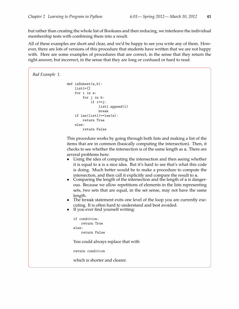
Chapter 2 Learning to Program in Python 6.01— Spring 2012—March 10, 2012 41
but rather than creating the whole list of Booleans and then reducing, we interleave the individualmembership tests with combining them into a result.
All of these examples are short and clear, and we’d be happy to see you write any of them. How-ever, there are lots of versions of this procedure that students have written that we are not happywith. Here are some examples of procedures that are correct, in the sense that they return theright answer, but incorrect, in the sense that they are long or confused or hard to read.
Bad Example 1.
def isSubset(a,b):list1=[]for i in a:
for j in b:if i==j:
list1.append(i)break
if len(list1)==len(a):return True
else:return False
This procedure works by going through both lists and making a list of theitems that are in common (basically computing the intersection). Then, itchecks to see whether the intersection is of the same length as a. There areseveral problems here:• Using the idea of computing the intersection and then seeing whether
it is equal to a is a nice idea. But it’s hard to see that’s what this codeis doing. Much better would be to make a procedure to compute theintersection, and then call it explicitly and compare the result to a.
• Comparing the length of the intersection and the length of a is danger-ous. Because we allow repetitions of elements in the lists representingsets, two sets that are equal, in the set sense, may not have the samelength.
• The break statement exits one level of the loop you are currently exe-cuting. It is often hard to understand and best avoided.
• If you ever find yourself writing:
if condition:return True
else:return False
You could always replace that with
return condition
which is shorter and clearer.

Chapter 2 Learning to Program in Python 6.01— Spring 2012—March 10, 2012 42
Bad Example 2.
def isSubset(a,b):itera = 0okay = Truewhile itera < len(a):
iterb = 0tempokay = Falsewhile iterb < len(b):
if a[itera] == b[iterb]:tempokay = True
iterb = iterb + 1if tempokay == False:
okay = Falseitera = itera + 1
return okay
This procedure is basically iterating over both lists, which is fine, but it isusing while rather than for to do so, which makes it hard to follow. Wecan rewrite it with for:
def isSubset(a,b):okay = Truefor itera in range(len(a)):
tempokay = Falsefor iterb in range(len(b)):
if a[itera] == b[iterb]:tempokay = True
if tempokay == False:okay = False
return okay
continued
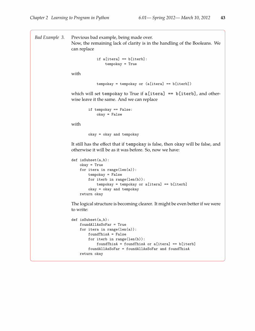
Chapter 2 Learning to Program in Python 6.01— Spring 2012—March 10, 2012 43
Bad Example 3. Previous bad example, being made over.Now, the remaining lack of clarity is in the handling of the Booleans. Wecan replace
if a[itera] == b[iterb]:tempokay = True
with
tempokay = tempokay or (a[itera] == b[iterb])
which will set tempokay to True if a[itera] == b[iterb], and other-wise leave it the same. And we can replace
if tempokay == False:okay = False
with
okay = okay and tempokay
It still has the effect that if tempokay is false, then okay will be false, andotherwise it will be as it was before. So, now we have:
def isSubset(a,b):okay = Truefor itera in range(len(a)):
tempokay = Falsefor iterb in range(len(b)):
tempokay = tempokay or a[itera] == b[iterb]okay = okay and tempokay
return okay
The logical structure is becoming clearer. It might be even better if we wereto write:
def isSubset(a,b):foundAllAsSoFar = Truefor itera in range(len(a)):
foundThisA = Falsefor iterb in range(len(b)):
foundThisA = foundThisA or a[itera] == b[iterb]foundAllAsSoFar = foundAllAsSoFar and foundThisA
return okay
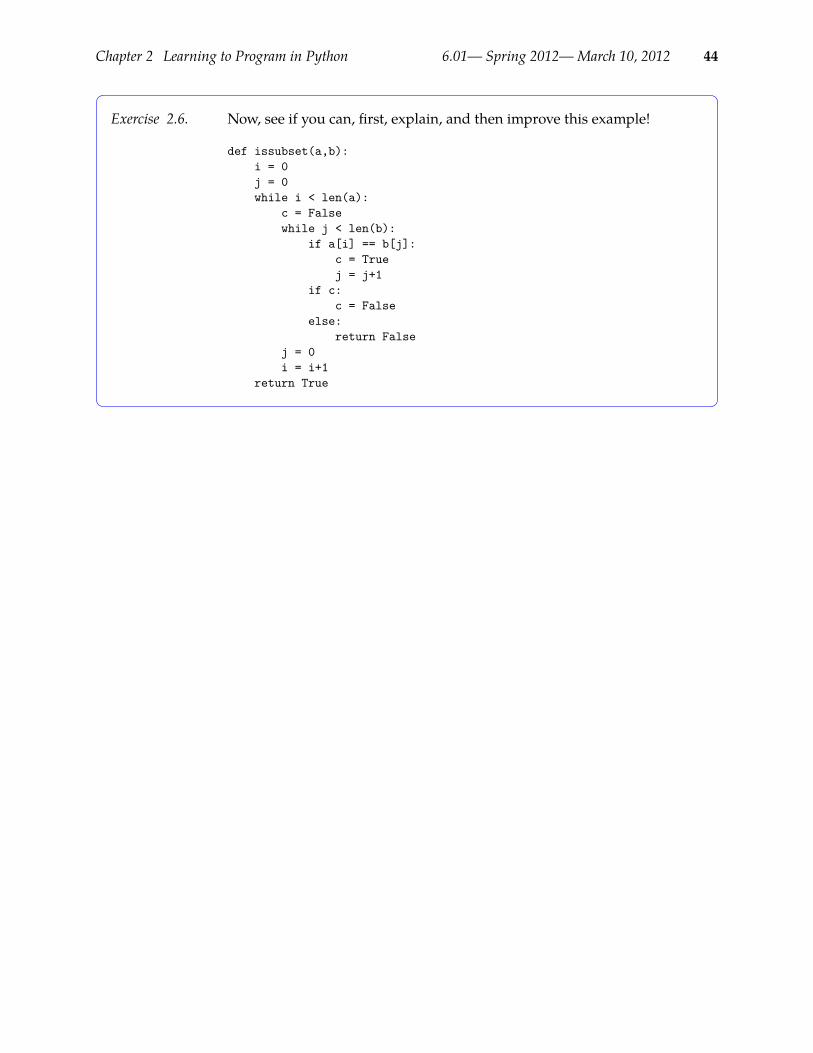
Chapter 2 Learning to Program in Python 6.01— Spring 2012—March 10, 2012 44
Exercise 2.6. Now, see if you can, first, explain, and then improve this example!
def issubset(a,b):i = 0j = 0while i < len(a):
c = Falsewhile j < len(b):
if a[i] == b[j]:c = Truej = j+1
if c:c = False
else:return False
j = 0i = i+1
return True

Chapter 3 Programs and Data 6.01— Spring 2012—March 10, 2012 45
Chapter 3Programs and Data
Object-oriented programming is a popular way of organizing programs, which groups togetherdata with the procedures that operate on them, thus facilitating some kinds of modularity andabstraction. In the context of our PCAP framework, object-oriented programming will give usmethods for capturing common patterns in data and the procedures that operate on that data, viaclasses, generic functions, and inheritance.
In this chapter, we will try to develop a deep understanding of object-oriented programming byworking through the mechanism bywhich an interpreter evaluates a computer program. The firstpart of the chapter will focus on interpretation of typical expxressions, starting from the simplestsingle-statement programs and working up through list structures and procedures. Many of theobservations made through this process apply to styles of program organization as well as object-oriented programming. Once we understand how an interpreter evaluates standard expressions,we will move to objects and classes. Although we use Python as an example, the discussion in thischapter is intended to be illustrative of principles of computer languages, more generally.
Inmany computer languages, including Python, programs are understood and executed by a com-puter program called an interpreter. Interpreters are surprisingly simple: the rules defining themeaning or semantics of a programming language are typically short and compact; and the inter-preter basically encodes these rules and applies them to any legal expressionn in the language.The enormous richness and complexity of computer programs comes from the composition ofprimitive elements with simple rules. The interpreter, in essence, defines the semantics of thelanguage by capturing the rules governing the value or behavior of program primitives, and ofwhat it means to combine the primitives in various ways. We will study the meaning of computerprograms by understanding how the interpreter operates on them.
An interpreter is made up of four pieces:• The reader or tokenizer takes as input a string of characters and divides them into tokens, which
are numbers (like -3.42), words (like while or a), and special characters (like :).• The parser takes as input the string of tokens and understands them as constructs in the pro-
gramming language, such as while loops, procedure definitions, or return statements.• The evaluator (which is also sometimes called the interpreter, as well) has the really interesting
job of determining the value and effects of the program that you ask it to interpret.• The printer takes the value returned by the evaluator and prints it out for the user to see.
Programs should never be a mystery to you: you can learn the simple semantic rules of the lan-guage and, if necessary, simulate what the interpreter would do, in order to understand any com-puter program which you are facing. Of course, in general, one does not want to work through

Chapter 3 Programs and Data 6.01— Spring 2012—March 10, 2012 46
the tedious process of simulating the interpreter, but this foundation of understanding the inter-preter’s process enables you to reason about the evaluation of any program.
3.1 Primitives, Composition, Abstraction, and PatternsWe will start by thinking about how the PCAP framework applies to computer programs, in gen-eral. We can do this by filling in table 3.1, exploring the PCAP ideas in data, procedures, andobjects.
DataThe primitive data items in most programming languages are things like integers, floating pointnumbers, and strings. We can combine these into data structures (we discuss some basic Pythondata structures in section 3.3) such as lists, arrays, dictionaries and records. Making a data struc-ture allows us, at the most basic level, to think of a collection of primitive data elements as if itwere one thing, freeing us from details. Sometimes, we just want to think of a collection of data,not in terms of its underlying representation, but in terms of what it represents. So, wemight wantto think of a set of objects, or a family tree, without worrying whether it is an array or a list in itsbasic representation. Abstract data types provide a way of abstracting away from representationaldetails and allowing us to focus on what the data really means.
ProceduresThe primitive procedures of a language are things like built-in numeric operations and basic listoperations. We can combine these using the facilities of the language, such as if and while, orby using function composition (f(g(x))). If we want to abstract away from the details of howa particular computation is done, we can define a new function; defining a function allows us touse it for computational jobs without thinking about the details of how those computational jobsget done. You can think of this process as essentially creating a new primitive, which we can thenuse while ignoring the details of how it is constructed. One way to capture common patterns ofabstraction in procedures is to abstract over procedures themselves, with higher-order procedures,which we discuss in detail in section 3.4.6.
ObjectsObject-oriented programming provides a number of methods of abstraction and pattern capturein both data and procedures. At the most basic level, objects can be used as records, combiningtogether primitive data elements. More generally, they provide strategies for jointly abstracting adata representation and the procedures that work on it. The features of inheritance and polymor-phism are particularly important, and we will discuss them in detail later in this chapter.
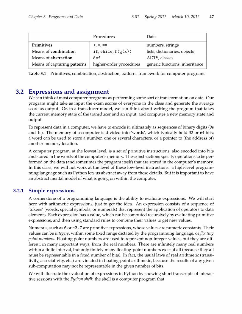
Chapter 3 Programs and Data 6.01— Spring 2012—March 10, 2012 47
Procedures Data
Primitives +, *, == numbers, stringsMeans of combination if, while, f(g(x)) lists, dictionaries, objectsMeans of abstraction def ADTS, classesMeans of capturing patterns higher-order procedures generic functions, inheritance
Table 3.1 Primitives, combination, abstraction, patterns framework for computer programs
3.2 Expressions and assignmentWe can think of most computer programs as performing some sort of transformation on data. Ourprogram might take as input the exam scores of everyone in the class and generate the averagescore as output. Or, in a transducer model, we can think about writing the program that takesthe current memory state of the transducer and an input, and computes a new memory state andoutput.
To represent data in a computer, we have to encode it, ultimately as sequences of binary digits (0sand 1s). The memory of a computer is divided into ’words’, which typically hold 32 or 64 bits;a word can be used to store a number, one or several characters, or a pointer to (the address of)another memory location.
A computer program, at the lowest level, is a set of primitive instructions, also encoded into bitsand stored in thewords of the computer’smemory. These instructions specify operations to be per-formed on the data (and sometimes the program itself) that are stored in the computer’s memory.In this class, we will not work at the level of these low-level instructions: a high-level program-ming language such as Python lets us abstract away from these details. But it is important to havean abstract mental model of what is going on within the computer.
3.2.1 Simple expressionsA cornerstone of a programming language is the ability to evaluate expressions. We will starthere with arithmetic expressions, just to get the idea. An expression consists of a sequence of’tokens’ (words, special symbols, or numerals) that represent the application of operators to dataelements. Each expression has a value, which can be computed recursively by evaluating primitiveexpressions, and then using standard rules to combine their values to get new values.
Numerals, such as 6 or -3.7 are primitive expressions, whose values are numeric constants. Theirvalues can be integers, within some fixed range dictated by the programming language, or floatingpoint numbers. Floating point numbers are used to represent non-integer values, but they are dif-ferent, in many important ways, from the real numbers. There are infinitely many real numberswithin a finite interval, but only finitely many floating-point numbers exist at all (because they allmust be representable in a fixed number of bits). In fact, the usual laws of real arithmetic (transi-tivity, associativity, etc.) are violated in floating-point arithmetic, because the results of any givensub-computation may not be representable in the given number of bits.
We will illustrate the evaluation of expressions in Python by showing short transcripts of interac-tive sessions with the Python shell: the shell is a computer program that

Chapter 3 Programs and Data 6.01— Spring 2012—March 10, 2012 48
• Prompts the user for an expression, by typing »>,• Reads what the user types in, and converts it into a set of tokens,• Parses the tokens into a data structure representing the syntax of the expression,• Evaluates the parsed expression using an interpreter, and• Prints out the resulting value
So, for example, we might have this interaction with Python:
>>> 2 + 35>>> (3 * 8) - 222>>> ((3 * 8) - 2) / 112>>> 2.02.0>>> 0.10.10000000000000001>>> 1.0 / 3.00.33333333333333331>>> 1 / 30
There are a couple of things to observe here. First, we can see how floating point numbers onlyapproximately represent real numbers: when we type in 0.1, the closest Python can come to it infloating point is 0.10000000000000001. The last interaction is particularly troubling: it seemslike the value of the expression 1 / 3 should be something like 0.33333. However, in Python, ifboth operands to the / operator are integers, then it will perform an integer division, truncatingany remainder.12
These expressions can be arbitrarily deeply nested combinations of primitives. The rules used forevaluation are essentially the same as the ones you learned in school; the interpreter proceeds byapplying the operations in precedence order13, evaluating sub-expressions to get new values, andthen evaluating the expressions those values participate in, until a single value results.
3.2.2 VariablesWe cannot go very far without variables. A variable is a name that we can bind to have a particularvalue and then later use in an expression. When a variable is encountered in an expression, it isevaluated by looking to see to what value it is bound.
An interpreter keeps track ofwhich variables are bound towhat values in binding environments. Anenvironment specifies a mapping between variable names and values. The values can be integers,floating-point numbers, characters, or pointers to more complex entities such as procedures orlarger collections of data.
Here is an example binding environment:
This behavior will no longer be the default in Python 3.0.12
Please Excuse My Dear Aunt Sally (Parentheses, Exponentiation, Multiplication, Division, Addition, Subtraction)13
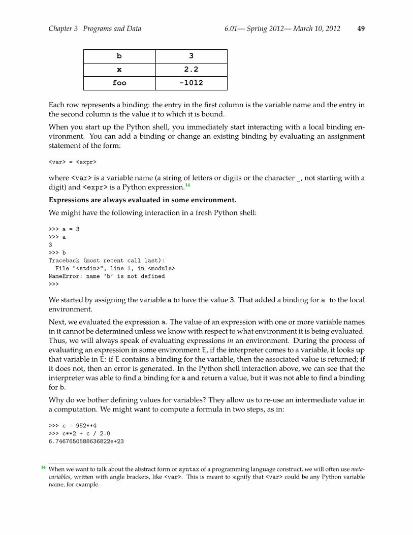
Chapter 3 Programs and Data 6.01— Spring 2012—March 10, 2012 49
-1012
2.2
3
foo
x
b
Each row represents a binding: the entry in the first column is the variable name and the entry inthe second column is the value it to which it is bound.
When you start up the Python shell, you immediately start interacting with a local binding en-vironment. You can add a binding or change an existing binding by evaluating an assignmentstatement of the form:
<var> = <expr>
where <var> is a variable name (a string of letters or digits or the character _, not starting with adigit) and <expr> is a Python expression.14
Expressions are always evaluated in some environment.
We might have the following interaction in a fresh Python shell:
>>> a = 3>>> a3>>> bTraceback (most recent call last):File "<stdin>", line 1, in <module>
NameError: name ’b’ is not defined>>>
We started by assigning the variable a to have the value 3. That added a binding for a to the localenvironment.
Next, we evaluated the expression a. The value of an expression with one or more variable namesin it cannot be determined unless we knowwith respect to what environment it is being evaluated.Thus, we will always speak of evaluating expressions in an environment. During the process ofevaluating an expression in some environment E, if the interpreter comes to a variable, it looks upthat variable in E: if E contains a binding for the variable, then the associated value is returned; ifit does not, then an error is generated. In the Python shell interaction above, we can see that theinterpreter was able to find a binding for a and return a value, but it was not able to find a bindingfor b.
Why do we bother defining values for variables? They allow us to re-use an intermediate value ina computation. We might want to compute a formula in two steps, as in:
>>> c = 952**4>>> c**2 + c / 2.06.7467650588636822e+23
When we want to talk about the abstract form or syntax of a programming language construct, we will often use meta-14
variables, written with angle brackets, like <var>. This is meant to signify that <var> could be any Python variablename, for example.
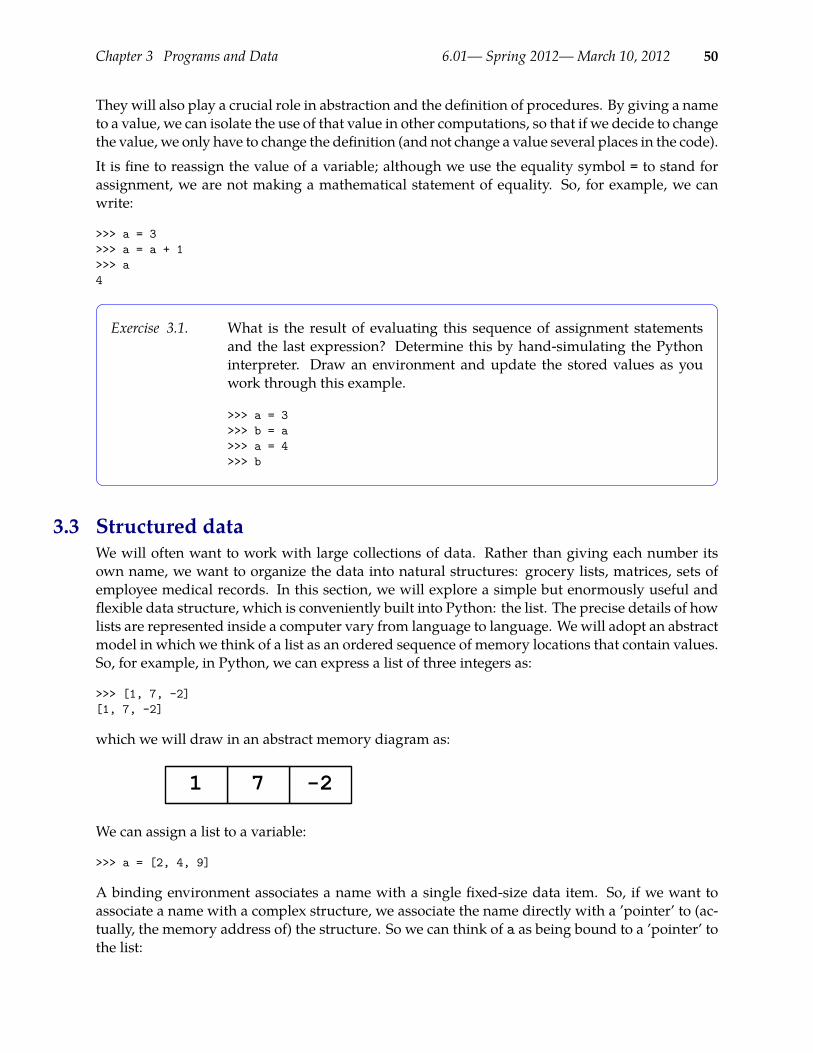
Chapter 3 Programs and Data 6.01— Spring 2012—March 10, 2012 50
They will also play a crucial role in abstraction and the definition of procedures. By giving a nameto a value, we can isolate the use of that value in other computations, so that if we decide to changethe value, we only have to change the definition (and not change a value several places in the code).It is fine to reassign the value of a variable; although we use the equality symbol = to stand forassignment, we are not making a mathematical statement of equality. So, for example, we canwrite:
>>> a = 3>>> a = a + 1>>> a4
Exercise 3.1. What is the result of evaluating this sequence of assignment statementsand the last expression? Determine this by hand-simulating the Pythoninterpreter. Draw an environment and update the stored values as youwork through this example.
>>> a = 3>>> b = a>>> a = 4>>> b
3.3 Structured dataWe will often want to work with large collections of data. Rather than giving each number itsown name, we want to organize the data into natural structures: grocery lists, matrices, sets ofemployee medical records. In this section, we will explore a simple but enormously useful andflexible data structure, which is conveniently built into Python: the list. The precise details of howlists are represented inside a computer vary from language to language. We will adopt an abstractmodel in which we think of a list as an ordered sequence of memory locations that contain values.So, for example, in Python, we can express a list of three integers as:
>>> [1, 7, -2][1, 7, -2]
which we will draw in an abstract memory diagram as:
-271
We can assign a list to a variable:
>>> a = [2, 4, 9]
A binding environment associates a name with a single fixed-size data item. So, if we want toassociate a name with a complex structure, we associate the name directly with a ’pointer’ to (ac-tually, the memory address of) the structure. So we can think of a as being bound to a ’pointer’ tothe list:
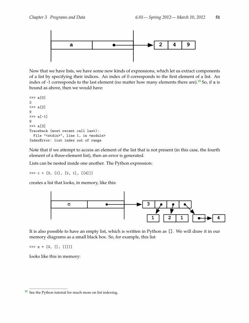
Chapter 3 Programs and Data 6.01— Spring 2012—March 10, 2012 51
a 942
Now that we have lists, we have some new kinds of expressions, which let us extract componentsof a list by specifying their indices. An index of 0 corresponds to the first element of a list. Anindex of -1 corresponds to the last element (no matter how many elements there are).15 So, if a isbound as above, then we would have:
>>> a[0]2>>> a[2]9>>> a[-1]9>>> a[3]Traceback (most recent call last):File "<stdin>", line 1, in <module>
IndexError: list index out of range
Note that if we attempt to access an element of the list that is not present (in this case, the fourthelement of a three-element list), then an error is generated.
Lists can be nested inside one another. The Python expression:
>>> c = [3, [1], [2, 1], [[4]]]
creates a list that looks, in memory, like this:
c 3
1 12 4
It is also possible to have an empty list, which is written in Python as []. We will draw it in ourmemory diagrams as a small black box. So, for example, this list
>>> z = [3, [], [[]]]
looks like this in memory:
See the Python tutorial for much more on list indexing.15
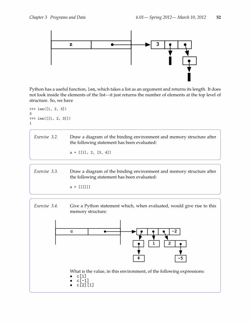
Chapter 3 Programs and Data 6.01— Spring 2012—March 10, 2012 52
z 3
Python has a useful function, len, which takes a list as an argument and returns its length. It doesnot look inside the elements of the list—it just returns the number of elements at the top level ofstructure. So, we have
>>> len([1, 2, 3])3>>> len([[1, 2, 3]])1
Exercise 3.2. Draw a diagram of the binding environment and memory structure afterthe following statement has been evaluated:
a = [[1], 2, [3, 4]]
Exercise 3.3. Draw a diagram of the binding environment and memory structure afterthe following statement has been evaluated:
a = [[[]]]
Exercise 3.4. Give a Python statement which, when evaluated, would give rise to thismemory structure:
c -2
1 2
4 -5
What is the value, in this environment, of the following expressions:• c[1]• c[-1]• c[2][1]

Chapter 3 Programs and Data 6.01— Spring 2012—March 10, 2012 53
3.3.1 List mutation and shared structureLists are mutable data structures, which means that we can actually change the values stored intheir elements. We do this by using element-selection expressions, like a[1] on the left-hand sideof an assignment statement. So, the assignment
a[1] = -3
assigns the second element of a to be -3. In more detail, the left-hand side of this expressionevaluates to a pointer to a specific location in memory (just as a’s value is a pointer to a location inmemory); then the assignment statement changes the value stored there by inserting the value ofthe right-hand side of the expression. If that statement were evaluated in this environment,
a 942
then the resulting environment would be:
a 9-32
We have permanently changed the list named a.
In this section, we will explore the consequences of the mutability of lists; programs that changelist structure can become very confusing, but you can always work your way through what ishappening by drawing out the memory diagrams.
Continuing the previous example, let us remember that a is bound directly to a pointer to a list(or a sequence of memory cells), and think about what happens if we do:
>>> b = a
Now, a and b are both names for the same list structure, resulting in a memory diagram like this:
ba 9-32
Now, we can reference parts of the list through b, and even change the list structure that way:
>>> b[0]2>>> b[2] = 1

Chapter 3 Programs and Data 6.01— Spring 2012—March 10, 2012 54
Notice that, because a and b point to the same list, changing b changes a!
>>> a[2, -3, 1]
Here is the memory picture now:
ba 1-32
This situation is called aliasing: the name b has become an alias for a. Aliasing can be useful, but itcan also cause problems, because youmight inadvertently change b (by passing it into a procedurethat changes one of its structured arguments, for example) when it is important to you to keep aunmodified.Another important way to change a list is to add or delete elements. We will demonstrate addingelements to the end of a list, but see the Python documentation for more operations on lists. Thisstatement
>>> a.append(9)
causes a new element to be added to the end of the list name a. The resulting memory state is:
ba 91-32
As before, because a and b are names for the same list (i.e., they point to the same memory se-quence), b is changed too. This is a side effect of the aliasing between a and b:
>>> b[2, -3, 1, 9]
Often, it will be important to make a fresh copy of a list so that you can change it without affect-ing the original one. Here are two equivalent ways to make a copy (use whichever one you canremember):
>>> c = list(a)>>> c = a[:]
Here is a picture of the memory at this point:
cba 91-32
91-32

Chapter 3 Programs and Data 6.01— Spring 2012—March 10, 2012 55
Now, if we change an element of c, it does not affect a (or b!):
>>> c[0] = 100>>> c[100, -3, 1, 9]>>> a[2, -3, 1, 9]
We can make crazy lists that share structure within a single list:
>>> f = [1, 2, 3]>>> g = [1, f, [f]]>>> g[1, [1, 2, 3], [[1, 2, 3]]]
which results in this memory structure:
gf 2 31
1
If you want to add an element to a list and get a new copy at the same time, you can do
>>> a + [1]
The + operator makes a new list that contains the elements of both of its arguments, but does notshare any top-level structure. All of our methods of copying only work reliably if your lists do notcontain other lists, because it only copies one level of list structure. So, for example, if we did:
>>> h = list(g)
we would end up with this picture:
hgf 2 31
1
1
It is clear that if we were to change f, it would change h, so this is not a completely new copy. Ifyou need to copy deep structures, that is, to make a copy not only of the top level list structure, butof the structures of any lists that list contains, and the lists those lists contain, etc., you will needto use the Python copy.deepcopy procedure.
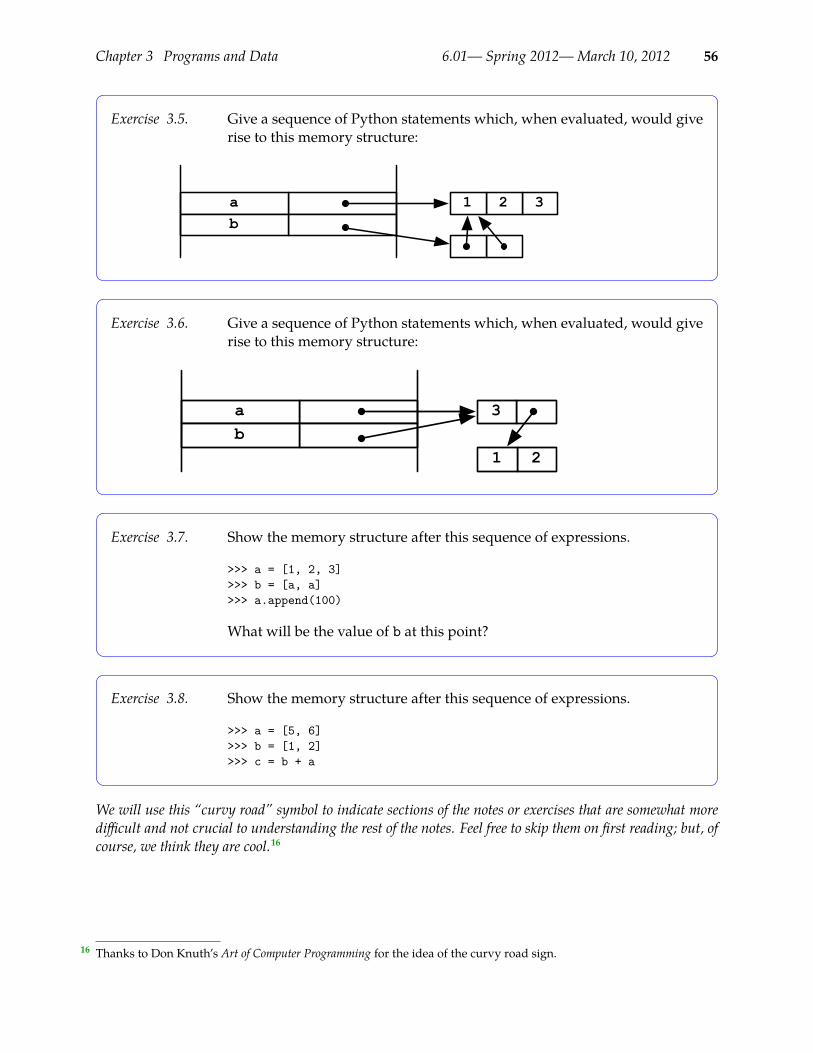
Chapter 3 Programs and Data 6.01— Spring 2012—March 10, 2012 56
Exercise 3.5. Give a sequence of Python statements which, when evaluated, would giverise to this memory structure:
ab
321
Exercise 3.6. Give a sequence of Python statements which, when evaluated, would giverise to this memory structure:
ab
3
21
Exercise 3.7. Show the memory structure after this sequence of expressions.
>>> a = [1, 2, 3]>>> b = [a, a]>>> a.append(100)
What will be the value of b at this point?
Exercise 3.8. Show the memory structure after this sequence of expressions.
>>> a = [5, 6]>>> b = [1, 2]>>> c = b + a
We will use this “curvy road” symbol to indicate sections of the notes or exercises that are somewhat moredifficult and not crucial to understanding the rest of the notes. Feel free to skip them on first reading; but, ofcourse, we think they are cool.16
Thanks to Don Knuth’s Art of Computer Programming for the idea of the curvy road sign.16

Chapter 3 Programs and Data 6.01— Spring 2012—March 10, 2012 57
Exercise 3.9.Show the memory structure after this sequence of expressions.
>>> a = [1, 2, 3]>>> a[1] = a
What will be the value of a at this point?
3.3.2 Tuples and stringsPython has two more list-like data types that are important to understand.
A tuple is a structure that is like a list, but is notmutable. You canmake new tuples, but you cannotchange the contents of a tuple or add elements to it. A tuple is typically written like a list, but withround parentheses instead of square ones:
>>> a = (1, 2, 3)
In fact, it is the commas and not the parentheses that matter here. So, you can write
>>> a = 1, 2, 3>>> a(1, 2, 3)
and still get a tuple. The only tricky thing about tuples is making a tuple with a single element.We could try
>>> a = (1)>>> a1
but it does not work, because in the expression (1) the parentheses are playing the standardgrouping role (and, in fact, because parentheses do not make tuples). So, to make a tuple witha single element, we have to use a comma:
>>> a = 1,>>> a(1,)
This is a little inelegant, but so it goes.
Tuples will be important in contexts where we are using structured objects as ’keys’, that is, toindex into another data structure, and where inconsistencies would occur if those keys could bechanged.
An important special kind of tuple is a string. A string can almost be thought of as a tuple ofcharacters. The details of what constitutes a character and how they are encoded is complicated,because modern character sets include characters from nearly all the world’s languages. We willstick to the characters we can type easily on our keyboards. In Python, you can write a string witheither single or double quotes: ’abc’ or "abc". You can select parts of it as you would a list:

Chapter 3 Programs and Data 6.01— Spring 2012—March 10, 2012 58
>>> s = ’abc’>>> s[0]’a’>>> s[-1]’c’
The strange thing about this is that s is a string, and because Python has no special data type torepresent a single character, s[0] is also a string.
We will frequently use + to concatenate two existing strings to make a new one:
>>> to = ’Jody’>>> fromP = ’Robin’>>> letter = ’Dear ’ + to + ",\n It’s over.\n" + fromP>>> print letterDear Jody,It’s over.
Robin
Aswell as using + to concatenate strings, this example illustrates several other small but importantpoints:• You can put a single quote inside a string that is delimited by double-quote characters (and viceversa).• If you want a new line in your string, you can write \n. Or, if you delimit your string with atriple quote, it can go over multiple lines.• The print statement can be used to print out results in your program.• Python, like most other programming languages, has some reserved words that have specialmeaning and cannot be used as variables. In this case, we wanted to use from, but that hasa special meaning to Python, so we used fromP instead.
Structured assignmentOnce we have lists and tuples, we can use a nice trick in assignment statements, based on thepacking and unpacking of tuples.
>>> a, b, c = 1, 2, 3>>> a1>>> b2>>> c3
Or, with lists,
>>> [a, b, c] = [1, 2, 3]>>> a1>>> b2>>> c3

Chapter 3 Programs and Data 6.01— Spring 2012—March 10, 2012 59
When you have a list (or a tuple) on the left-hand side of an assignment statement, you have tohave a list (or tuple) of matching structure on the right-hand side. Then Python will “unpack”them both, and assign to the individual components of the structure on the left hand side. Youcan get fancier with this method:
>>> thing = [8, 9, [1, 2], ’John’, [33.3, 44.4]]>>> [a, b, c, d, [e1, e2]] = thing>>> c[1, 2]>>> e133.299999999999997
3.4 ProceduresProcedures are computer-program constructs that let us capture common patterns of computationby:• Gathering together sequences of statements• Abstracting away from particular data items on which they operate.
Here is a procedure definition,17 and then its use:
def square(x):return x * x
>>> square(6)36>>> square(2 - square(2))4
We will work through, in detail, what happens when the interpreter evaluates a procedure defin-ition, and then the application of that procedure.
3.4.1 DefinitionA procedure definition has the abstract form:
def <name>(<fp1>, ..., <fpn>):<statement1>...<statementk>
There are essentially three parts:• <name> is a name for the procedure, with the same restrictions as a variable name;• <fp1>, ..., <fpn> is a list of formal parameters, which will stand for the data items on whichthis procedure will operate; and
In the code displayed in these notes, we will show procedures being defined and then used, as if the definitions were17
happening in the Python shell (but without the prompts). In fact, you should not type procedure definitions into theshell, because if you make a mistake, you will have to re-type the whole thing, and because multi-line objects are nothandled very well. Instead, type your procedure definitions into a file in Idle, and then test them by ’running’ the file inIdle (which will actually evaluate all of the expressions in your file) and then evaluating test expressions in Idle’s shell.
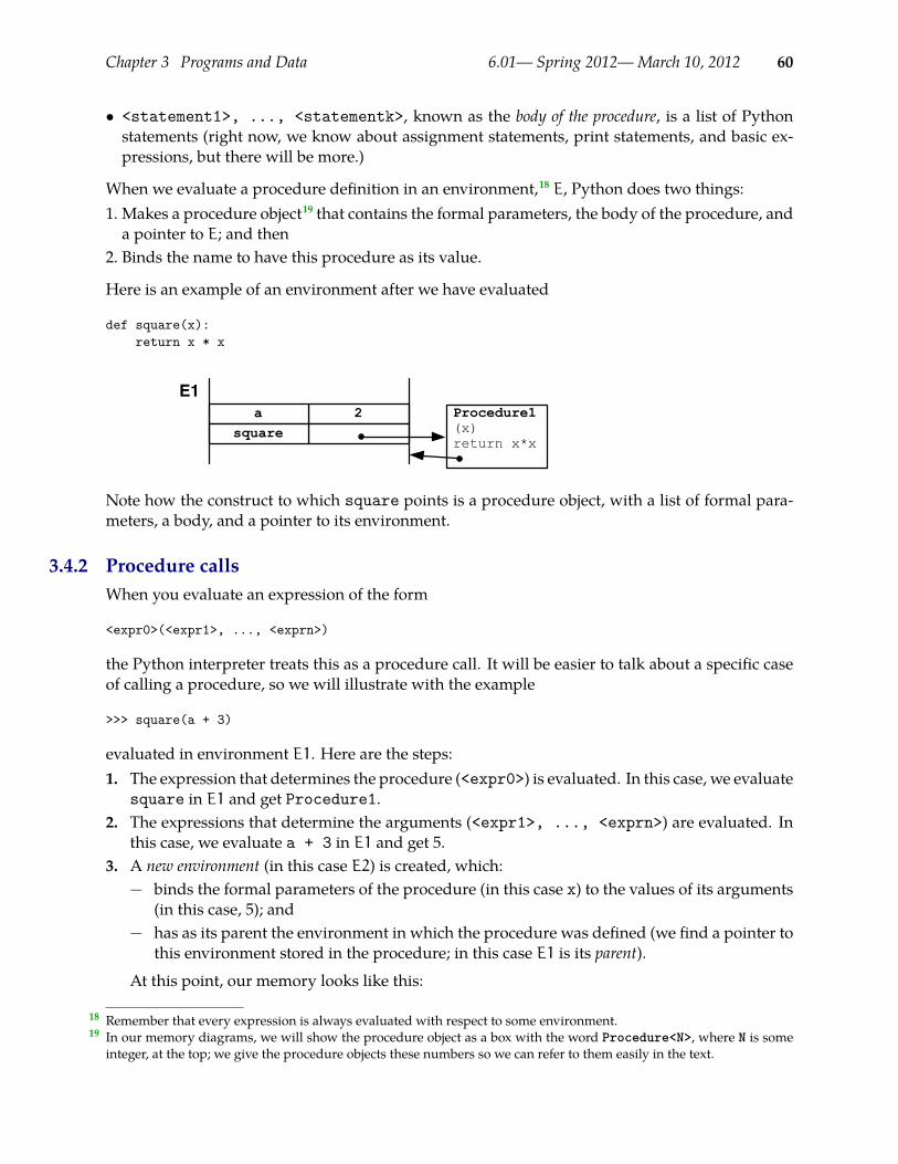
Chapter 3 Programs and Data 6.01— Spring 2012—March 10, 2012 60
• <statement1>, ..., <statementk>, known as the body of the procedure, is a list of Pythonstatements (right now, we know about assignment statements, print statements, and basic ex-pressions, but there will be more.)
When we evaluate a procedure definition in an environment,18 E, Python does two things:1. Makes a procedure object19 that contains the formal parameters, the body of the procedure, anda pointer to E; and then
2. Binds the name to have this procedure as its value.
Here is an example of an environment after we have evaluated
def square(x):return x * x
2asquare
Procedure1(x)return x*x
E1
Note how the construct to which square points is a procedure object, with a list of formal para-meters, a body, and a pointer to its environment.
3.4.2 Procedure callsWhen you evaluate an expression of the form
<expr0>(<expr1>, ..., <exprn>)
the Python interpreter treats this as a procedure call. It will be easier to talk about a specific caseof calling a procedure, so we will illustrate with the example
>>> square(a + 3)
evaluated in environment E1. Here are the steps:1. The expression that determines the procedure (<expr0>) is evaluated. In this case, we evaluate
square in E1 and get Procedure1.2. The expressions that determine the arguments (<expr1>, ..., <exprn>) are evaluated. In
this case, we evaluate a + 3 in E1 and get 5.3. A new environment (in this case E2) is created, which:
− binds the formal parameters of the procedure (in this case x) to the values of its arguments(in this case, 5); and
− has as its parent the environment in which the procedure was defined (we find a pointer tothis environment stored in the procedure; in this case E1 is its parent).
At this point, our memory looks like this:
Remember that every expression is always evaluated with respect to some environment.18
In our memory diagrams, we will show the procedure object as a box with the word Procedure<N>, where N is some19
integer, at the top; we give the procedure objects these numbers so we can refer to them easily in the text.
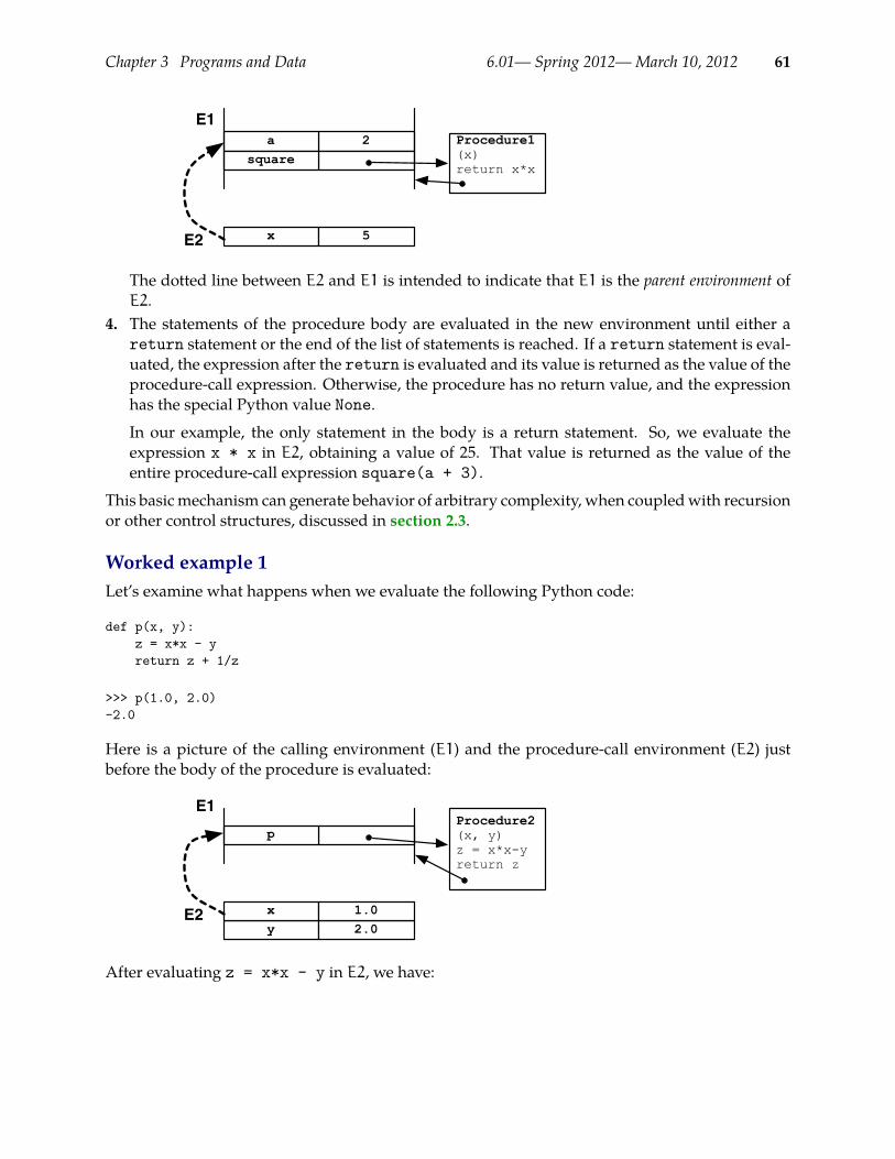
Chapter 3 Programs and Data 6.01— Spring 2012—March 10, 2012 61
2asquare
Procedure1(x)return x*x
E1
x 5E2
The dotted line between E2 and E1 is intended to indicate that E1 is the parent environment ofE2.
4. The statements of the procedure body are evaluated in the new environment until either areturn statement or the end of the list of statements is reached. If a return statement is eval-uated, the expression after the return is evaluated and its value is returned as the value of theprocedure-call expression. Otherwise, the procedure has no return value, and the expressionhas the special Python value None.
In our example, the only statement in the body is a return statement. So, we evaluate theexpression x * x in E2, obtaining a value of 25. That value is returned as the value of theentire procedure-call expression square(a + 3).
This basicmechanism can generate behavior of arbitrary complexity, when coupledwith recursionor other control structures, discussed in section 2.3.
Worked example 1Let’s examine what happens when we evaluate the following Python code:
def p(x, y):z = x*x - yreturn z + 1/z
>>> p(1.0, 2.0)-2.0
Here is a picture of the calling environment (E1) and the procedure-call environment (E2) justbefore the body of the procedure is evaluated:
pProcedure2(x, y)z = x*x-yreturn z
E1
y 2.0x 1.0E2
After evaluating z = x*x - y in E2, we have:

Chapter 3 Programs and Data 6.01— Spring 2012—March 10, 2012 62
p
Procedure2(x, y)z = x*x-yreturn z+1/z
E1
-1.0zy 2.0x 1.0E2
Finally, we evaluate z + 1/z in E2 and get -2.0, which we return.
Worked example 2Here is another example:
def silly(a):a = a + 1return a
>>> b = 6>>> silly(b)7
Here is a picture of the calling environment (E1) and the procedure-call environment (E2) justbefore the body of the procedure is evaluated:
6bsilly
Procedure3(a)a=a+1return a
E1
a 6E2
After evaluating a = a + 1 in E2, we have:
b 6silly
Procedure3(a)a=a+1return a
E1
a 7E2
Finally, we evaluate a in E2 and get 7, which we return.
Convince yourself that the execution below works fine, and notice that having a binding for a inE2means that we leave the binding for a in E1 unmolested:
>>> a = 2>>> silly(a)3
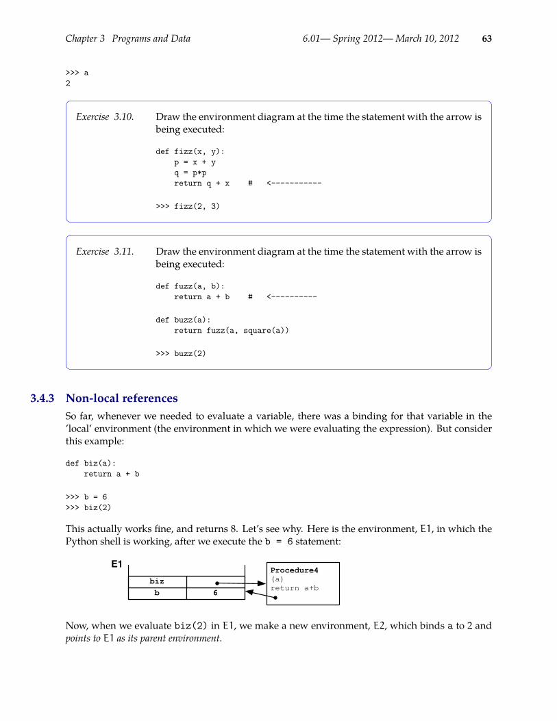
Chapter 3 Programs and Data 6.01— Spring 2012—March 10, 2012 63
>>> a2
Exercise 3.10. Draw the environment diagram at the time the statement with the arrow isbeing executed:
def fizz(x, y):p = x + yq = p*preturn q + x # <-----------
>>> fizz(2, 3)
Exercise 3.11. Draw the environment diagram at the time the statement with the arrow isbeing executed:
def fuzz(a, b):return a + b # <----------
def buzz(a):return fuzz(a, square(a))
>>> buzz(2)
3.4.3 Non-local referencesSo far, whenever we needed to evaluate a variable, there was a binding for that variable in the’local’ environment (the environment in which we were evaluating the expression). But considerthis example:
def biz(a):return a + b
>>> b = 6>>> biz(2)
This actually works fine, and returns 8. Let’s see why. Here is the environment, E1, in which thePython shell is working, after we execute the b = 6 statement:
b 6biz
Procedure4(a)return a+b
E1
Now, when we evaluate biz(2) in E1, we make a new environment, E2, which binds a to 2 andpoints to E1 as its parent environment.
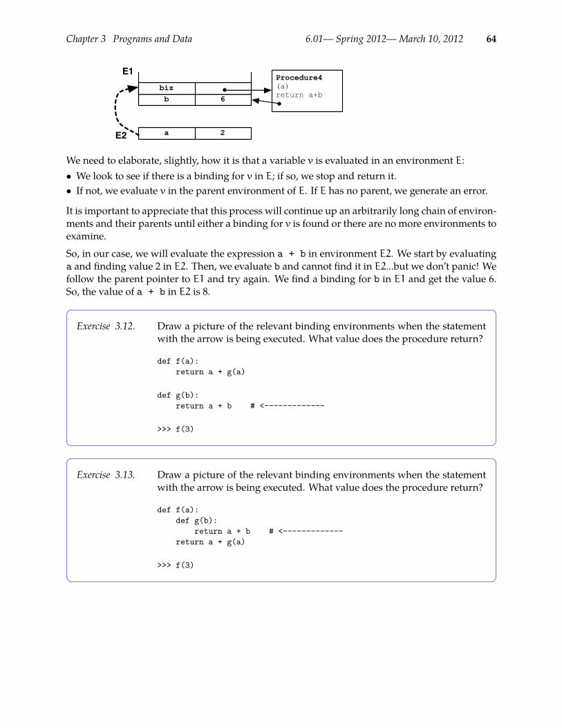
Chapter 3 Programs and Data 6.01— Spring 2012—March 10, 2012 64
b 6biz
Procedure4(a)return a+b
E1
a 2E2
We need to elaborate, slightly, how it is that a variable v is evaluated in an environment E:• We look to see if there is a binding for v in E; if so, we stop and return it.• If not, we evaluate v in the parent environment of E. If E has no parent, we generate an error.
It is important to appreciate that this process will continue up an arbitrarily long chain of environ-ments and their parents until either a binding for v is found or there are no more environments toexamine.
So, in our case, we will evaluate the expression a + b in environment E2. We start by evaluatinga and finding value 2 in E2. Then, we evaluate b and cannot find it in E2...but we don’t panic! Wefollow the parent pointer to E1 and try again. We find a binding for b in E1 and get the value 6.So, the value of a + b in E2 is 8.
Exercise 3.12. Draw a picture of the relevant binding environments when the statementwith the arrow is being executed. What value does the procedure return?
def f(a):return a + g(a)
def g(b):return a + b # <-------------
>>> f(3)
Exercise 3.13. Draw a picture of the relevant binding environments when the statementwith the arrow is being executed. What value does the procedure return?
def f(a):def g(b):
return a + b # <-------------return a + g(a)
>>> f(3)
Chapter 3 Programs and Data 6.01— Spring 2012—March 10, 2012 65
Exercise 3.14. Draw a picture of the relevant binding environments when the statementwith the arrow is being executed. What value does the procedure return?Does it cause an error?
def a(a):return a * a
>>> a(2)
3.4.4 Environments in PythonGenerally, Python establishes the following binding environments:1. __builtin__: the mother of all environments: it contains the definitions of all sorts of basic
symbols, like list and sum. It is the parent of all module environments.2. Module: each separate file that contains Python code is called amodule and establishes its own
environment, whose parent is __builtin__.3. Procedure calls: as described in this section. A procedure that is defined at the ’top level’ of a
module (that is, not nested in the definition of another procedure) has the module’s environ-ment as its parent, and has its name defined in the module’s environment. Procedures thatare defined inside other procedures have the procedure-call environment of the containingprocedure as their parent.
We have seen two operations that cause bindings to be created: assignments and procedure calls.Bindings are also created when you evaluate an import statement. If you evaluate
import math
then a file associated with the math module is evaluated and the name math is bound, in thecurrent environment, to the math module, which is an environment. No other names are addedto the current environment, and if you want to refer to names in that module, you have to qualifythem, as in math.sqrt. (As we will see in a subsequent section, the evaluation of this expressionfirst evaluates math, which returns an environment. We can then evaluate sqrt with respect tothat environment, thus returning a pointer to the procedure stored there.) If you execute
from math import sqrt
then the math file is evaluated, and the name sqrt is bound, in the current environment, to what-ever the name sqrt is bound in the math module. But note that if you do this, the name math isnot bound to anything, and you cannot access any other procedures in the math module unlessyou import them explicitly, as well.
3.4.5 Non-local references in proceduresThere is an important subtlety in the way names are handled in the environment created by aprocedure call. When a name that is not bound in the local environment is referenced, then it islooked up in the chain of parent environments. So, as we have seen, it is fine to have

Chapter 3 Programs and Data 6.01— Spring 2012—March 10, 2012 66
a = 2def b():
return a
When a name is assigned inside a procedure, a new binding is created for it in the environmentassociated with the current call of that procedure. So, it is fine to have
a = 2def b():
a = 3c = 4return a + c
Both assignments cause new bindings to be made in the local environment, and it is those bind-ings that are used to supply values in the return expression. It will not change a in the globalenvironment.
But here is a code fragment that causes trouble:
a = 3def b():
a = a + 1print a
It seems completely reasonable, and you might expect b() to return 4. But, instead, it generatesan error. What is going on?? It all has to do with when Python decides to add a binding to thelocal environment. When it sees this procedure definition, it sees that the name a occurs on theleft-hand-side of an assignment statement, and so, at the very beginning, it puts a new entry for ain the local environment, but without any value bound to it. Now, when it is time to evaluate thestatement
a = a + 1
Python starts by evaluating the expression on the right hand side: a + 1. When it tries to look upthe name a in the procedure-call environment, it finds that a has been added to the environment,but has not yet had a value specified. So it generates an error.
In Python, we can write code to increment a number named in the global environment, by usingthe global declaration:
a = 3def b():
global aa = a + 1print a
>>> b()4>>> b()5>>> a5
Chapter 3 Programs and Data 6.01— Spring 2012—March 10, 2012 67
The statement global a asks that a new binding for a not be made in the procedure-call envi-ronment. Now, all references to a are to the binding in the module’s environment, and so thisprocedure actually changes a.
In Python, we can only make assignments to names in the procedure-call environment or to themodule environment, but not to names in intermediate environments. So, for example,
def outer():def inner():
a = a + 1a = 0inner()
In this example, we get an error, because Python has made a new binding for a in the environmentfor the call to inner. We would really like inner to be able to see and modify the a that belongsto the environment for outer, but there is no way to arrange this. Some other programminglanguages, such as Scheme, offer more fine-grained control over how the scoping of variables ishandled.
3.4.6 Procedures as first-class objectsIn Python, unlikemanyother languages, procedures are treated inmuch the sameway as numbers:they can be stored as values of variables, can be passed as arguments to procedures, and canbe returned as results of procedure calls. Because of this, we say that procedures are treated as“first-class” objects. We will explore this treatment of “higher-order” procedures (procedures thatmanipulated procedures) throughout this section.
First of all, it is useful to see that we can construct (some) procedures without naming them usingthe lambda constructor:
lambda <var1>, ..., <varn> : <expr>
The formal parameters are <var1>, ..., <varn> and the body is <expr>. There is no need foran explicit return statement; the value of the expression is always returned. A single expressioncan only be one line of Python, such as you could put on the right hand side of an assignmentstatement. Here are some examples:
>>> f = lambda x: x*x>>> f<function <lambda> at 0x4ecf0>>>> f(4)16
Here is a procedure of two arguments defined with lambda:
>>> g = lambda x,y : x * y>>> g(3, 4)12
Using the expression-evaluation rules we have already established, we can do some fancy thingswith procedures, which we will illustrate throughout the rest of this section.

Chapter 3 Programs and Data 6.01— Spring 2012—March 10, 2012 68
>>> procs = [lambda x: x, lambda x: x + 1, lambda x: x + 2]>>> procs[0]<function <lambda> at 0x83d70>>>> procs[1](6)7
Here, we have defined a list of three procedures. We can see that an individual element of the list(e.g., procs[0]) is a procedure.20 So, then procs[1](6) applies the second procedure in the listto the argument 6. Since the second procedure returns its argument plus 1, the result is 7.
Here is a demonstration that procedures can be assigned to names in just the way other valuescan.
>>> fuzz = procs[2]>>> fuzz(3)5
def thing(a):return a * a
>>> thing(3)9>>> thang = thing>>> thang(3)9
Passing procedures as argumentsJust as we can pass numbers or lists into procedures as arguments, we can pass in procedures asarguments, as well.
What if we find that we are often wanting to perform the same procedure twice on an argument?That is, we seem to keep writing square(square(x)). If it were always the same procedure wewere applying twice, we could just write a new procedure
def squaretwice(x):return square(square(x))
But what if it is different procedures? We can write a new procedure that takes a procedure f asan argument and applies it twice:
def doTwice(f, x):return f(f(x))
So, if we wanted to square twice, we could do:
>>> doTwice(square,2)16
Here is a picture of the environment structure in place when we are evaluating the returnf(f(x)) statement in doTwice:
In the programming world, people often use the words “function” and “procedure” either interchangeable or with20
minor subtle distinctions. The Python interpreter refers to the objects we are calling procedures as “functions.”

Chapter 3 Programs and Data 6.01— Spring 2012—March 10, 2012 69
doTwice
square
E1
2xf
E2
Procedure5(x)return x * x
Procedure6(f, x)return f(f(x))
Environment E1 is the module environment, where procedures square and doTwice were de-fined and where the expression doTwice(square, 2) is being evaluated. The interpreter:• Evaluates doTwice in E1 and gets Procedure6.• Evaluates square in E1 and gets Procedure5.• Evaluates 2 in E1 and gets 2.• Makes the new binding environment E2, binding the formal parameters, f and x, of Procedure6, to actual arguments Procedure5 and 2.• Evaluates the body of Procedure6 in E2.
Now, let’s peek one level deeper into the process. To evaluate f(f(x)) in E2, the interpreter startsby evaluating the inner f(x) expression. It• Evaluates f in E2 and gets Procedure5.• Evaluates x in E2 and gets 2.• Makes the new binding environment E3, binding the formal parameter x, of Procedure5, to 2.(Remember that the parent of E3 is E1 because Procedure5 has E1 as a parent.)• Evaluates the body of Procedure5 in E3, getting 4.
The environments at the time of this last evaluation step are:
doTwice
square
E1
2xf
E2
Procedure5(x)return x * x
Procedure6(f, x)return f(f(x))
2xE3
A similar thing happens when we evaluate the outer application of f, but now with argument 4,and a return value of 16.
Chapter 3 Programs and Data 6.01— Spring 2012—March 10, 2012 70
Exercise 3.15. Here is the definition of a procedure sumOfProcs that takes two proce-dures, f and g, as well as another value x, as arguments, and returns f(x)+ g(x). The sumOfProcs procedure is then applied to two little test pro-cedures:
def sumOfProcs(f, g, x):return f(x) + g(x)
def thing1(a):return a*a*a
def thing2(b):return b+1 # <--------------------
>>> sumOfProcs(thing1, thing2, 2)
Draw a picture of all of the relevant environments at the moment the state-ment with the arrow is being evaluated. What is the return value of the callto sumOfProcs?
Returning procedures as valuesAnother way to apply a procedure multiple times is this:
def doTwiceMaker(f):return lambda x: f(f(x))
This is a procedure that returns a procedure! If you would rather not use lambda, you could writeit this way:
def doTwiceMaker(f):def twoF(x):
return f(f(x))return twoF
Now, to use doTwiceMaker, we might start by calling it with a procedure, such as square, as anargument and naming the resulting procedure.
>>> twoSquare = doTwiceMaker(square)
Here is a picture of the environments just before the return twoF statement in doTwiceMaker isevaluated.
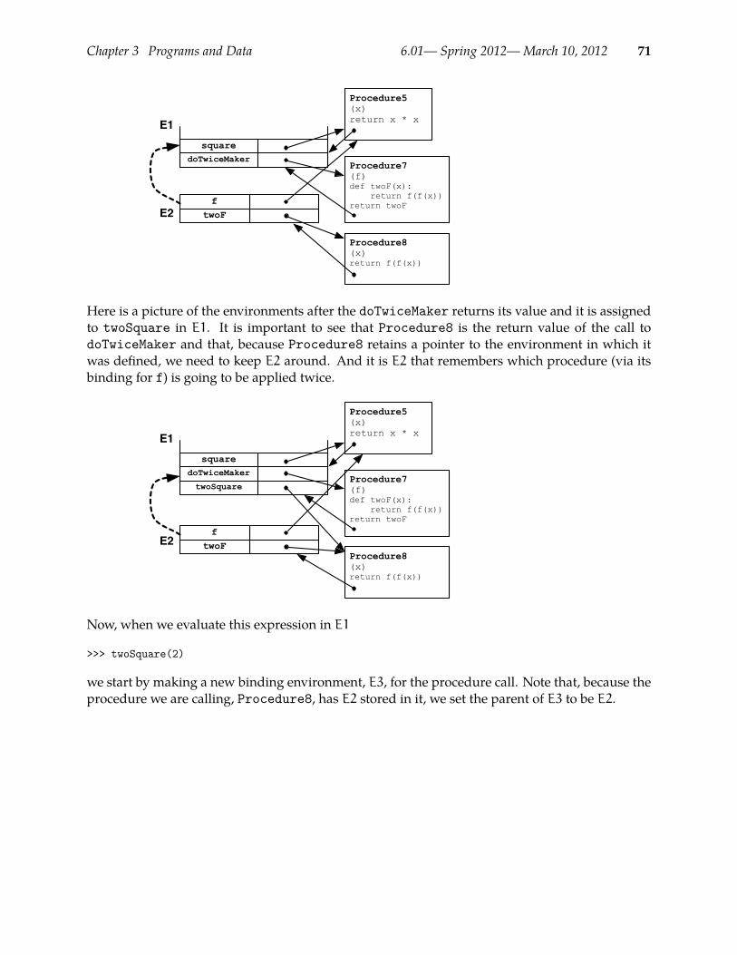
Chapter 3 Programs and Data 6.01— Spring 2012—March 10, 2012 71
doTwiceMaker
square
E1
twoFf
E2
Procedure5(x)return x * x
Procedure7(f)def twoF(x): return f(f(x))return twoF
Procedure8(x)return f(f(x))
Here is a picture of the environments after the doTwiceMaker returns its value and it is assignedto twoSquare in E1. It is important to see that Procedure8 is the return value of the call todoTwiceMaker and that, because Procedure8 retains a pointer to the environment in which itwas defined, we need to keep E2 around. And it is E2 that remembers which procedure (via itsbinding for f) is going to be applied twice.
twoSquare
doTwiceMaker
square
E1
twoFf
E2
Procedure5(x)return x * x
Procedure7(f)def twoF(x): return f(f(x))return twoF
Procedure8(x)return f(f(x))
Now, when we evaluate this expression in E1
>>> twoSquare(2)
we start by making a new binding environment, E3, for the procedure call. Note that, because theprocedure we are calling, Procedure8, has E2 stored in it, we set the parent of E3 to be E2.
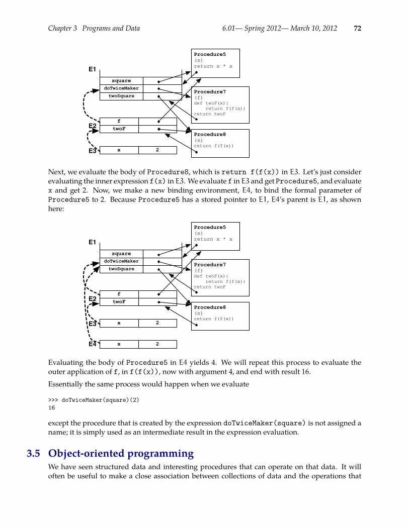
Chapter 3 Programs and Data 6.01— Spring 2012—March 10, 2012 72
twoSquare
doTwiceMaker
square
E1
twoFf
E2
Procedure5(x)return x * x
Procedure7(f)def twoF(x): return f(f(x))return twoF
Procedure8(x)return f(f(x))
2xE3
Next, we evaluate the body of Procedure8, which is return f(f(x)) in E3. Let’s just considerevaluating the inner expression f(x) inE3. We evaluate f inE3 and get Procedure5, and evaluatex and get 2. Now, we make a new binding environment, E4, to bind the formal parameter ofProcedure5 to 2. Because Procedure5 has a stored pointer to E1, E4’s parent is E1, as shownhere:
twoSquare
doTwiceMaker
square
E1
twoFf
E2
Procedure5(x)return x * x
Procedure7(f)def twoF(x): return f(f(x))return twoF
Procedure8(x)return f(f(x))
2xE3
2xE4
Evaluating the body of Procedure5 in E4 yields 4. We will repeat this process to evaluate theouter application of f, in f(f(x)), now with argument 4, and end with result 16.
Essentially the same process would happen when we evaluate
>>> doTwiceMaker(square)(2)16
except the procedure that is created by the expression doTwiceMaker(square) is not assigned aname; it is simply used as an intermediate result in the expression evaluation.
3.5 Object-oriented programmingWe have seen structured data and interesting procedures that can operate on that data. It willoften be useful to make a close association between collections of data and the operations that

Chapter 3 Programs and Data 6.01— Spring 2012—March 10, 2012 73
apply to them. The style of programming that takes this point of view is object-oriented programming(OOP). It requires adding some simple mechanisms to our interpreter, but is not a big conceptualdeparture from the things we have already seen. It is, however, a different style of organizing largeprograms.
3.5.1 Classes and instancesIn OOP, we introduce the idea of classes and instances. An instance is a collection of data that de-scribe a single entity in our domain of interest, such as a person or a car or a point in 3D space. Ifwe have many instances that share some data values, or upon which we would want to performsimilar operations, then we can represent them as being members of a class and store the sharedinformation once with the class, rather than replicating it in the instances.
Consider the following staff database for a large undergraduate course:
name role age building room course
Pat Prof 60 34 501 6.01Kelly TA 31 34 501 6.01Lynn TA 29 34 501 6.01Dana LA 19 34 501 6.01Chris LA 20 34 501 6.01
There are lots of shared values here, so we might want to define a class. A class definition has theform:
class <name>:<statement1>...<statementn>
Here is the definition of simple class in our example domain:
class Staff601:course = ’6.01’building = 34room = 501
From the implementation perspective, the most important thing to know is that classes and in-stances are environments.
When we define a new class, we make a new environment. In this case, the act of defining classStaff601 in an environment E1 results in a binding from Staff601 to E2, an empty environmentwhose parent is E1, the environment in which the class definition was evaluated. Now, the state-ments inside the class definition are evaluated in the new environment, resulting in a memorystate like this:21
In fact, the string ’6.01’ should be shown as an external memory structure, with a pointer stored in the binding en-21
vironment; for compactness in the following diagrams we will sometimes show the strings themselves as if they werestored directly in the environment.
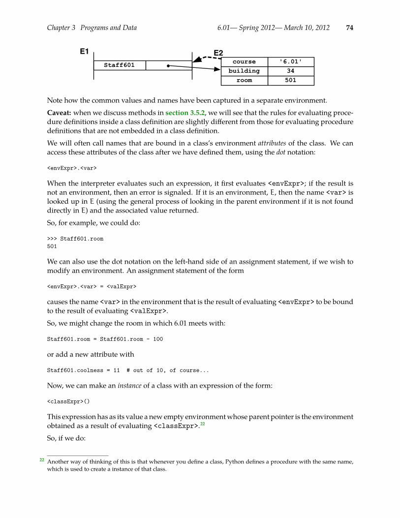
Chapter 3 Programs and Data 6.01— Spring 2012—March 10, 2012 74
Staff601
E1
501room34building
'6.01'courseE2
Note how the common values and names have been captured in a separate environment.
Caveat: when we discuss methods in section 3.5.2, we will see that the rules for evaluating proce-dure definitions inside a class definition are slightly different from those for evaluating proceduredefinitions that are not embedded in a class definition.
We will often call names that are bound in a class’s environment attributes of the class. We canaccess these attributes of the class after we have defined them, using the dot notation:
<envExpr>.<var>
When the interpreter evaluates such an expression, it first evaluates <envExpr>; if the result isnot an environment, then an error is signaled. If it is an environment, E, then the name <var> islooked up in E (using the general process of looking in the parent environment if it is not founddirectly in E) and the associated value returned.
So, for example, we could do:
>>> Staff601.room501
We can also use the dot notation on the left-hand side of an assignment statement, if we wish tomodify an environment. An assignment statement of the form
<envExpr>.<var> = <valExpr>
causes the name <var> in the environment that is the result of evaluating <envExpr> to be boundto the result of evaluating <valExpr>.
So, we might change the room in which 6.01 meets with:
Staff601.room = Staff601.room - 100
or add a new attribute with
Staff601.coolness = 11 # out of 10, of course...
Now, we can make an instance of a class with an expression of the form:
<classExpr>()
This expression has as its value a newempty environmentwhose parent pointer is the environmentobtained as a result of evaluating <classExpr>.22
So, if we do:
Another way of thinking of this is that whenever you define a class, Python defines a procedure with the same name,22
which is used to create a instance of that class.
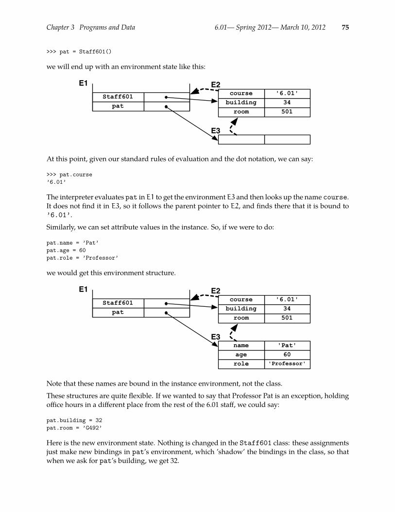
Chapter 3 Programs and Data 6.01— Spring 2012—March 10, 2012 75
>>> pat = Staff601()
we will end up with an environment state like this:
patStaff601
E1
501room34building
'6.01'courseE2
E3
At this point, given our standard rules of evaluation and the dot notation, we can say:
>>> pat.course’6.01’
The interpreter evaluates pat in E1 to get the environment E3 and then looks up the name course.It does not find it in E3, so it follows the parent pointer to E2, and finds there that it is bound to’6.01’.
Similarly, we can set attribute values in the instance. So, if we were to do:
pat.name = ’Pat’pat.age = 60pat.role = ’Professor’
we would get this environment structure.
patStaff601
E1
501room34building
'6.01'courseE2
'Professor'role60age
'Pat'nameE3
Note that these names are bound in the instance environment, not the class.
These structures are quite flexible. If we wanted to say that Professor Pat is an exception, holdingoffice hours in a different place from the rest of the 6.01 staff, we could say:
pat.building = 32pat.room = ’G492’
Here is the new environment state. Nothing is changed in the Staff601 class: these assignmentsjust make new bindings in pat’s environment, which ’shadow’ the bindings in the class, so thatwhen we ask for pat’s building, we get 32.
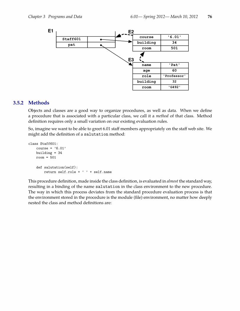
Chapter 3 Programs and Data 6.01— Spring 2012—March 10, 2012 76
patStaff601
E1
501room34building
'6.01'courseE2
'G492'room32building
'Professor'role60age
'Pat'nameE3
3.5.2 MethodsObjects and classes are a good way to organize procedures, as well as data. When we definea procedure that is associated with a particular class, we call it a method of that class. Methoddefinition requires only a small variation on our existing evaluation rules.
So, imagine we want to be able to greet 6.01 staff members appropriately on the staff web site. Wemight add the definition of a salutationmethod:
class Staff601:course = ’6.01’building = 34room = 501
def salutation(self):return self.role + ’ ’ + self.name
This procedure definition, made inside the class definition, is evaluated in almost the standardway,resulting in a binding of the name salutation in the class environment to the new procedure.The way in which this process deviates from the standard procedure evaluation process is thatthe environment stored in the procedure is the module (file) environment, no matter how deeplynested the class and method definitions are:
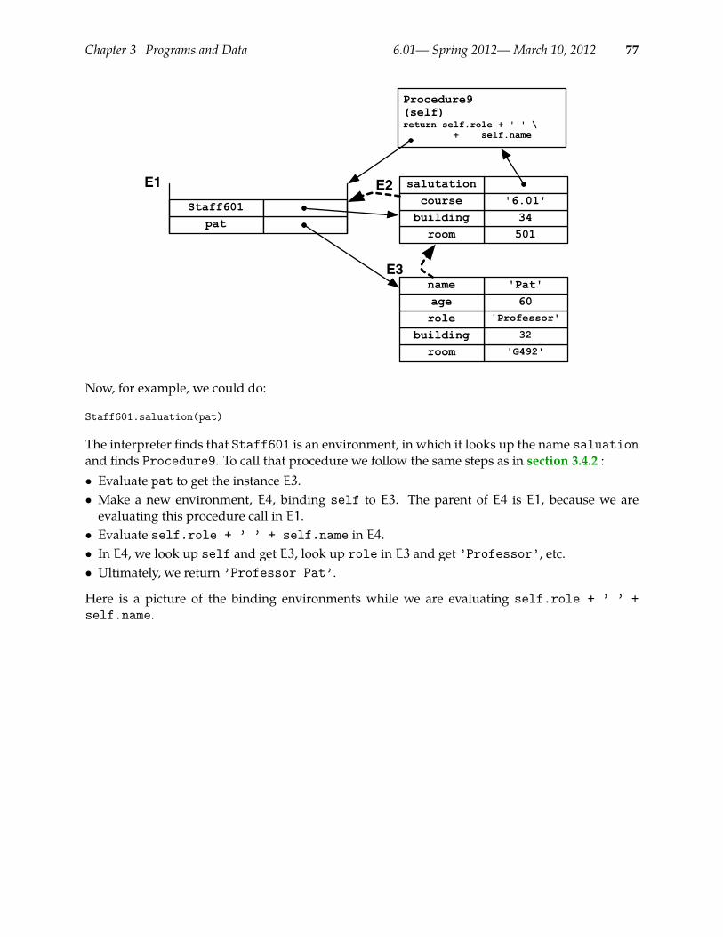
Chapter 3 Programs and Data 6.01— Spring 2012—March 10, 2012 77
patStaff601
E1 salutation
501room34building
'6.01'courseE2
'G492'room32building
'Professor'role60age
'Pat'nameE3
Procedure9(self)return self.role + ' ' \ + self.name
Now, for example, we could do:
Staff601.saluation(pat)
The interpreter finds that Staff601 is an environment, in which it looks up the name saluationand finds Procedure9. To call that procedure we follow the same steps as in section 3.4.2 :• Evaluate pat to get the instance E3.• Make a new environment, E4, binding self to E3. The parent of E4 is E1, because we areevaluating this procedure call in E1.• Evaluate self.role + ’ ’ + self.name in E4.• In E4, we look up self and get E3, look up role in E3 and get ’Professor’, etc.• Ultimately, we return ’Professor Pat’.
Here is a picture of the binding environments while we are evaluating self.role + ’ ’ +self.name.
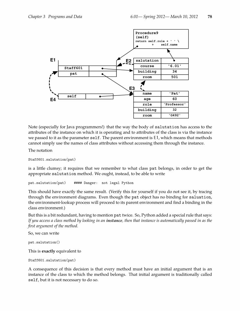
Chapter 3 Programs and Data 6.01— Spring 2012—March 10, 2012 78
patStaff601
E1 salutation
501room34building
'6.01'courseE2
'G492'room32building
'Professor'role60age
'Pat'nameE3
Procedure9(self)return self.role + ' ' \ + self.name
selfE4
Note (especially for Java programmers!) that the way the body of salutation has access to theattributes of the instance on which it is operating and to attributes of the class is via the instancewe passed to it as the parameter self. The parent environment is E1, which means that methodscannot simply use the names of class attributes without accessing them through the instance.The notation
Staff601.salutation(pat)
is a little clumsy; it requires that we remember to what class pat belongs, in order to get theappropriate salutationmethod. We ought, instead, to be able to write
pat.salutation(pat) #### Danger: not legal Python
This should have exactly the same result. (Verify this for yourself if you do not see it, by tracingthrough the environment diagrams. Even though the pat object has no binding for saluation,the environment-lookup process will proceed to its parent environment and find a binding in theclass environment.)But this is a bit redundant, having tomention pat twice. So, Python added a special rule that says:If you access a class method by looking in an instance, then that instance is automatically passed in as thefirst argument of the method.So, we can write
pat.salutation()
This is exactly equivalent to
Staff601.salutation(pat)
A consequence of this decision is that every method must have an initial argument that is aninstance of the class to which the method belongs. That initial argument is traditionally calledself, but it is not necessary to do so.
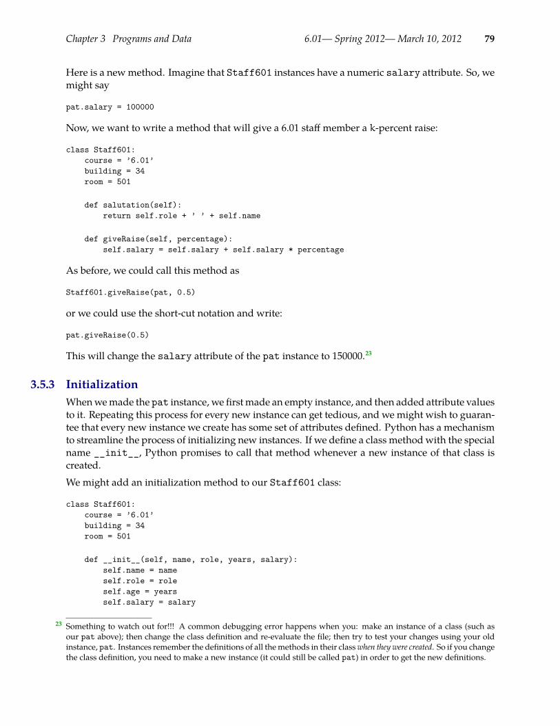
Chapter 3 Programs and Data 6.01— Spring 2012—March 10, 2012 79
Here is a newmethod. Imagine that Staff601 instances have a numeric salary attribute. So, wemight say
pat.salary = 100000
Now, we want to write a method that will give a 6.01 staff member a k-percent raise:
class Staff601:course = ’6.01’building = 34room = 501
def salutation(self):return self.role + ’ ’ + self.name
def giveRaise(self, percentage):self.salary = self.salary + self.salary * percentage
As before, we could call this method as
Staff601.giveRaise(pat, 0.5)
or we could use the short-cut notation and write:
pat.giveRaise(0.5)
This will change the salary attribute of the pat instance to 150000.23
3.5.3 InitializationWhenwemade the pat instance, we firstmade an empty instance, and then added attribute valuesto it. Repeating this process for every new instance can get tedious, and we might wish to guaran-tee that every new instance we create has some set of attributes defined. Python has a mechanismto streamline the process of initializing new instances. If we define a class methodwith the specialname __init__, Python promises to call that method whenever a new instance of that class iscreated.
We might add an initialization method to our Staff601 class:
class Staff601:course = ’6.01’building = 34room = 501
def __init__(self, name, role, years, salary):self.name = nameself.role = roleself.age = yearsself.salary = salary
Something to watch out for!!! A common debugging error happens when you: make an instance of a class (such as23
our pat above); then change the class definition and re-evaluate the file; then try to test your changes using your oldinstance, pat. Instances remember the definitions of all themethods in their classwhen they were created. So if you changethe class definition, you need to make a new instance (it could still be called pat) in order to get the new definitions.
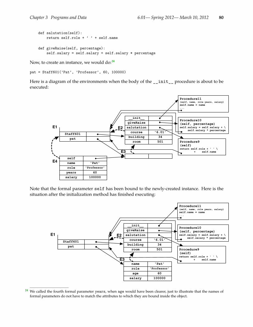
Chapter 3 Programs and Data 6.01— Spring 2012—March 10, 2012 80
def salutation(self):return self.role + ’ ’ + self.name
def giveRaise(self, percentage):self.salary = self.salary + self.salary * percentage
Now, to create an instance, we would do:24
pat = Staff601(’Pat’, ’Professor’, 60, 100000)
Here is a diagram of the environments when the body of the __init__ procedure is about to beexecuted:
patStaff601
E1
__init__giveRaisesalutation
501room34building
'6.01'courseE2
E3
Procedure9(self)return self.role + ' ' \ + self.name
salary 10000060years
role 'Professor'
name 'Pat'self
E4
Procedure11(self, name, role years, salary)self.name = name...
Procedure10(self, percentage)self.salary = self.salary + \ self.salary * percentage
Note that the formal parameter self has been bound to the newly-created instance. Here is thesituation after the initialization method has finished executing:
patStaff601
E1
__init__giveRaisesalutation
501room34building
'6.01'courseE2
salary 100000age 60role 'Professor'
'Pat'nameE3
Procedure9(self)return self.role + ' ' \ + self.name
Procedure11(self, name, role years, salary)self.name = name...
Procedure10(self, percentage)self.salary = self.salary + \ self.salary * percentage
We called the fourth formal parameter years, when age would have been clearer, just to illustrate that the names of24
formal parameters do not have to match the attributes to which they are bound inside the object.
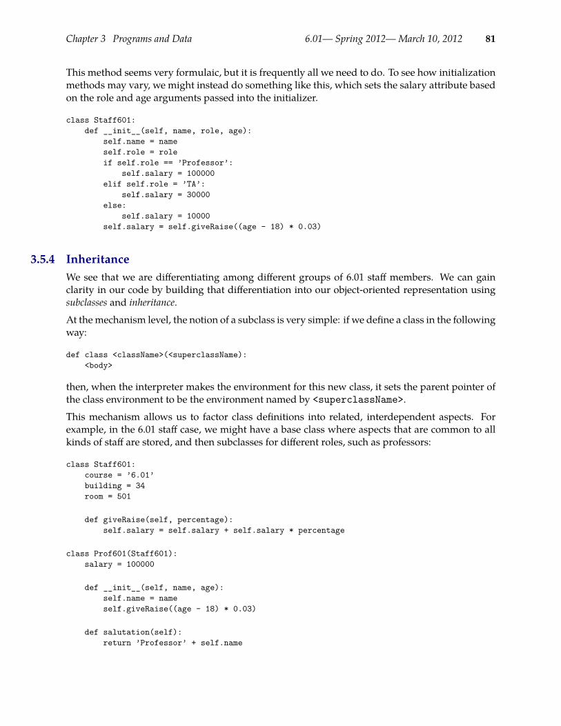
Chapter 3 Programs and Data 6.01— Spring 2012—March 10, 2012 81
This method seems very formulaic, but it is frequently all we need to do. To see how initializationmethods may vary, we might instead do something like this, which sets the salary attribute basedon the role and age arguments passed into the initializer.
class Staff601:def __init__(self, name, role, age):
self.name = nameself.role = roleif self.role == ’Professor’:
self.salary = 100000elif self.role = ’TA’:
self.salary = 30000else:
self.salary = 10000self.salary = self.giveRaise((age - 18) * 0.03)
3.5.4 InheritanceWe see that we are differentiating among different groups of 6.01 staff members. We can gainclarity in our code by building that differentiation into our object-oriented representation usingsubclasses and inheritance.
At themechanism level, the notion of a subclass is very simple: if we define a class in the followingway:
def class <className>(<superclassName):<body>
then, when the interpreter makes the environment for this new class, it sets the parent pointer ofthe class environment to be the environment named by <superclassName>.
This mechanism allows us to factor class definitions into related, interdependent aspects. Forexample, in the 6.01 staff case, we might have a base class where aspects that are common to allkinds of staff are stored, and then subclasses for different roles, such as professors:
class Staff601:course = ’6.01’building = 34room = 501
def giveRaise(self, percentage):self.salary = self.salary + self.salary * percentage
class Prof601(Staff601):salary = 100000
def __init__(self, name, age):self.name = nameself.giveRaise((age - 18) * 0.03)
def salutation(self):return ’Professor’ + self.name

Chapter 3 Programs and Data 6.01— Spring 2012—March 10, 2012 82
Let’s trace what happens when we make a new instance of Prof601with the expression
Prof601(’Pat’, 60)
First a new environment, E4, is constructed, with E3 (the environment associated with the classProf601 as its parent). Here is the memory picture now:
patProf601Staff601
E1giveRaise
501room34building
'6.01'courseE2
E3
Procedure9(self)return 'Professor ' \ + self.name
salutation
salary 100000__init__
Procedure11(self, name, age)self.name = nameself.raise((age-18)*0.03)
Procedure10(self, percentage)self.salary = self.salary + \ self.salary * percentage
E4
As soon as it is created, the __init__ method is called, with the new environment E4 as its firstparameter and the rest of its parameters obtained by evaluating the expressions that were passedinto to Prof601, in this case, ’Pat’ and 60. Now, we need to make the procedure-call environ-ment, binding the formal parameters of Procedure11; it is E5 in this figure:
patProf601Staff601
E1giveRaise
501room34building
'6.01'course
E2
E3
Procedure9(self)return 'Professor ' \ + self.name
salutation
salary 100000__init__
Procedure11(self, name, age)self.name = nameself.raise((age-18)*0.03)
Procedure10(self, percentage)self.salary = self.salary + \ self.salary * percentage
E460age
name 'Pat'self
E5
We evaluate the body of Procedure11 in E5. It starts straightforwardly by evaluating
self.name = name
which creates a binding from name to ’Pat’ in the object named self, which is E4. Now, itevaluates
self.giveRaise((age - 18) * 0.03)
in E5. It starts by evaluating self.giveRaise. self is E4, so we look for a binding of giveRaise.It is not bound in E4, so we look in the parent E3; it is not bound in E3 so we look in E2 and find
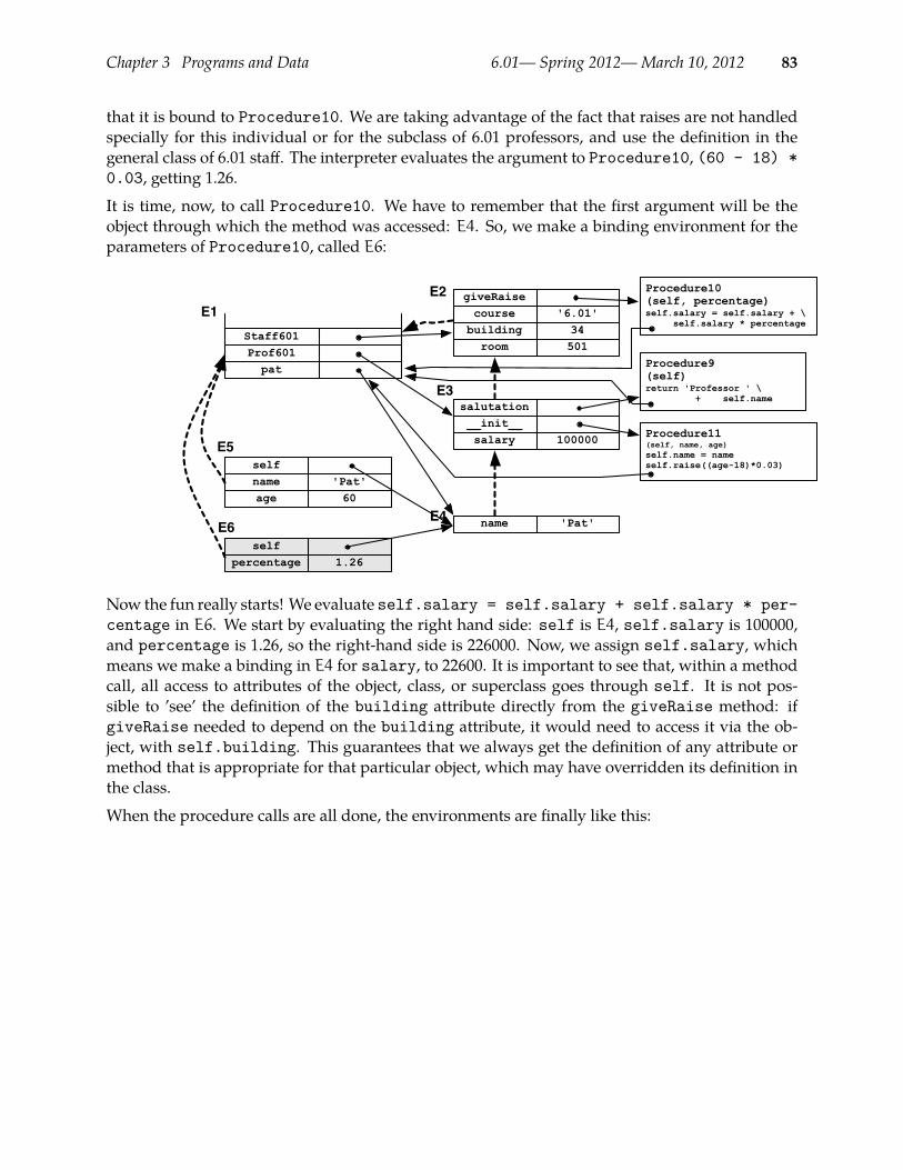
Chapter 3 Programs and Data 6.01— Spring 2012—March 10, 2012 83
that it is bound to Procedure10. We are taking advantage of the fact that raises are not handledspecially for this individual or for the subclass of 6.01 professors, and use the definition in thegeneral class of 6.01 staff. The interpreter evaluates the argument to Procedure10, (60 - 18) *0.03, getting 1.26.
It is time, now, to call Procedure10. We have to remember that the first argument will be theobject through which the method was accessed: E4. So, we make a binding environment for theparameters of Procedure10, called E6:
patProf601Staff601
E1giveRaise
501room34building
'6.01'course
E2
E3
Procedure9(self)return 'Professor ' \ + self.name
salutation
salary 100000__init__
Procedure11(self, name, age)self.name = nameself.raise((age-18)*0.03)
Procedure10(self, percentage)self.salary = self.salary + \ self.salary * percentage
'Pat'nameE460age
name 'Pat'self
E5
percentage 1.26self
E6
Now the fun really starts! We evaluate self.salary = self.salary + self.salary * per-centage in E6. We start by evaluating the right hand side: self is E4, self.salary is 100000,and percentage is 1.26, so the right-hand side is 226000. Now, we assign self.salary, whichmeans we make a binding in E4 for salary, to 22600. It is important to see that, within a methodcall, all access to attributes of the object, class, or superclass goes through self. It is not pos-sible to ’see’ the definition of the building attribute directly from the giveRaise method: ifgiveRaise needed to depend on the building attribute, it would need to access it via the ob-ject, with self.building. This guarantees that we always get the definition of any attribute ormethod that is appropriate for that particular object, which may have overridden its definition inthe class.
When the procedure calls are all done, the environments are finally like this:

Chapter 3 Programs and Data 6.01— Spring 2012—March 10, 2012 84
patProf601Staff601
E1giveRaise
501room34building
'6.01'course
E2
E3
Procedure9(self)return 'Professor ' \ + self.name
salutation
salary 100000__init__
Procedure11(self, name, age)self.name = nameself.raise((age-18)*0.03)
Procedure10(self, percentage)self.salary = self.salary + \ self.salary * percentage
'Pat'salary 226000nameE4
It is useful to back up and see the structure here:• The instance pat is an environment, E4.• The parent of the instance is an environment,E3, which is the class Prof601.• The parent of the class is an environment, E2, which the superclass Staff601.
3.5.5 Using InheritanceFrequently when we’re using inheritance, we override some methods of a parent class, and usesome of its methods unchanged. Occasionally, we will want to modify or augment an existingmethod from the parent class. In such a situation, we can ’wrap’ that method by writing ourown version of that method in the child class, but calling the method of the parent to do some ofthe work. To call a method bar from a parent class named Foo, you can do something like thefollowing.
def SubclassOfFoo(Foo):def bar(self, arg):
Foo.bar(self, arg)
When you call a method using the class name, rather than an object name, you need to pass theobject in explicitly to the method call.Here is a concrete example. Imagine that you have a class for managing calendars. It has thesemethods, plus possibly some others.
class Calendar:def __init__(self):
self.appointments = []def makeAppointment(self, name, dateTime):
self.appointments.append((name, dateTime))def printCalendar(self, start, end):
# complicated stuff
Now, you’d like to make a calendar that can handle appointments that are made in different timezones. It should store all of the appointments in a single time zone, so that it can sort and displayappropriately.
Chapter 3 Programs and Data 6.01— Spring 2012—March 10, 2012 85
class CalendarTimeZone(Calendar):def __init__(self, zone):
Calendar.__init__(self)self.zone = zone
def makeAppointment(self, name, dateTime):Calendar.makeAppointment(self, name, dateTime + self.zone)
Wemake a subclass of Calendarwhich takes a time zone zone as an argument to its initializationmethod. It starts by calling the Calendar initialization method, to set up whatever internal datastructures are necessary, and then sets the zone attribute of the new object. Now, when it’s timeto make an appointment, we add the time zone offset to the appointed time, and then call themakeAppointmentmethod of Calendar.
What is nice about this example is that we were able to take advantage of the Calendar class, andeven add to some of its methods, without knowing anything about its internal representation ofcalendars.
3.6 RecursionThere are many control structures in Python, and other modern languages, which allow youwriteshort programs that do a lot of work. In this section, we discuss recursion, which is also a way towrite programs of arbitrary complexity. It is of particular importance here, because the structureof a language interpreter is recursive, and in the next section we will explore, in detail, how toconstruct an interpreter.
We have seen how we can define a procedure, and then can use it without remembering or caringabout the details of how it is implemented. We sometimes say that we can treat it as a black box,meaning that it is unnecessary to look inside it to use it. This is crucial for maintaining sanitywhen building complex pieces of software. An even more interesting case is when we can thinkof the procedure that we are in the middle of defining as a black box. That is what we do whenwe write a recursive procedure.
Recursive procedures are ways of doing a lot of work. The amount of work to be done is controlledby one or more arguments to the procedure. The way we are going to do a lot of work is by callingthe procedure, over and over again, from inside itself! The way wemake sure this process actuallyterminates is by being sure that the argument that controls how much work we do gets smallerevery time we call the procedure again. The argument might be a number that counts down tozero, or a string or list that gets shorter.
There are two parts to writing a recursive procedure: the base case(s) and the recursive case. Thebase case happens when the thing that is controlling howmuchwork you do has gotten to its small-est value; usually this is 0 or the empty string or list, but it can be anything, as long as you knowit is sure to happen. In the base case, you just compute the answer directly (no more calls to therecursive procedure!) and return it. Otherwise, you are in the recursive case. In the recursive case,you try to be as lazy as possible, and foist most of thework off on another call to this procedure, butwith one of its arguments getting smaller. Then, when you get the answer back from the recursivecall, you do some additional work and return the result.
Another way to think about it is this: when you are given a problem of size n, assume someonealready gave you a way to solve problems of size n− 1. So, now, your job is only to figure out
Chapter 3 Programs and Data 6.01— Spring 2012—March 10, 2012 86
• To which problem of size n− 1 you would like to know the answer, and• How to do some simple operations to make that answer into the answer to your problem of sizen.
What if you wanted to add two positive numbers, but your computer only had the ability to incre-ment and decrement (add and subtract 1)? You could do this recursively, by thinking about it likethis. I need to add m and n:• Presupposing the ability to solve simpler problems, I could get the answer to the problem m plusn-1.• Now, I just need to add 1 to that answer, to get the answer to my problem.
We further need to reason that when n is 0, then the answer is just m. This leads to the followingPython definition:
def slowAdd(m, n):if n == 0:
return melse:
return 1 + slowAdd(m, n-1)
Note how in the final return expression, we have reduced the answer to a problem of size n to asimpler version of the same problem (of size n-1 plus some simple operations.
Here is an example recursive procedure that returns a string of n 1’s:
def bunchaOnes(n):if n == 0:
return ’’else:
return bunchaOnes(n-1) + ’1’
The thing that is getting smaller is n. In the base case, we just return the empty string. In therecursive case, we get someone else to figure out the answer to the question of n-1 ones, and thenwe just do a little additional work (adding one more ’1’ to the end of the string) and return it.
Exercise 3.16. What is the result of evaluating
bunchaOnes(-5)
Here is another example. It is kind of a crazy way to do multiplication, but logicians love it.
def mult(a,b):if a==0:
return 0else:
return b + mult(a-1,b)
Trace through an example of what happens when you call mult(3, 4), by adding a print state-ment that prints arguments a and b as the first line of the procedure, and seeing what happens.

Chapter 3 Programs and Data 6.01— Spring 2012—March 10, 2012 87
Here is a more interesting example of recursion. Imagine we wanted to compute the binary repre-sentation of an integer. For example, the binary representation of 145 is ’10010001’. Our procedurewill take an integer as input, and return a string of 1’s and 0’s.
def bin(n):if n == 0:
return ’0’elif n == 1:
return ’1’else:
return bin(n/2) + bin(n%2)
The easy cases (base cases) are whenwe are down to a 1 or a 0, in which case the answer is obvious.If we do not have an easy case, we divide up our problem into two that are easier. So, if we convertn/2 (the integer result of dividing n by 2, which by Python’s definition will be a smaller numbersince it truncates the result, throwing away any remainder), into a string of digits, we will haveall but the last digit. And n%2 (n modulo 2) is 1 or 0 depending on whether the number is evenor odd, so one more call of bin will return a string of ’0’ or ’1’. The other thing that is importantto remember is that the + operation here is being used for string concatenation, not addition ofnumbers.
How do we know that this procedure is going to terminate? We know that the number on whichit is operating is a positive integer that is getting smaller and smaller, and will eventually be eithera 1 or a 0, which can be handled by the base case.
You can also do recursion on lists. Here a way to add up the values of a list of numbers:
def addList(elts):if elts == []:
return 0else:
return elts[0] + addList(elts[1:])
The addList procedure consumed a list and produced a number. The incrementElements pro-cedure below shows how to use recursion to do something to every element of a list and make anew list containing the results.
def incrementElements(elts):if elts == []:
return []else:
return [elts[0]+1] + incrementElements(elts[1:])
If the list of elements is empty, then there is no work to be done, and the result is just the emptylist. Otherwise, the result is a new list: the first element of the new list is the first element of theold list, plus 1; the rest of the new list is the result of calling incrementElement recursively onthe rest of the input list. Because the list we are operating on is getting shorter on every recursivecall, we know we will reach the base case, and all will be well.
3.7 Implementing an interpreter
Chapter 3 Programs and Data 6.01— Spring 2012—March 10, 2012 88
This section can be skipped unless you are interested. It’s very cool but a bit tricky.
From the preceding sections, you should have an informal understanding of what happenswhen a Python program is evaluated. Now, we want to understand it formally enough to actuallyimplement an interpreter in Python.
3.7.1 SpyWe will study a simplified language, which we call Spy, because it is a mixture of Scheme andPython. From Scheme, an elegant interpreted programming language with very simple syntaxand semantics, we take the syntax of the language, and from Python, we take the basic object-oriented programming system. Spy has a small subset of the features of these languages, but itis powerful enough to implement any computer program that can be implemented in any otherlanguage (though it could be mighty tedious).
To learn more: Interestingly, very minimal versions of several different models of compu-tation (imperative, functional/recursive, rewrite systems) have been shownto be formally equivalent. Some have theorized them to be complete in thesense that there are no computations that cannot be expressed this way. Formore information, see:http://plato.stanford.edu/entries/church-turing/
The syntax of Spy, like Scheme, is fully-parenthesized prefix syntax. Prefix means that the name ofthe function or operation comes before its arguments, and fully-parenthesized means that there areparentheses around every sub-expression. So, to write 1 + num * 4, we would write
(+ 1 (* num 4)) .
The reason for adopting this syntax is that it is very easy to manipulate with a computer program(although some humans find it hard to read). In the following, we will assume that someonehas already written a tokenizer, which is a program that can consume a stream of characters andbreak it into “words” for us. In particular, we will assume that the tokenizer can break an inputSpy program down into a list of lists (of lists...of elements that are strings or integers). So theexpression (+ 1 (* num 4))would be converted by the tokenizer into a representation such as:(’+’, 1, (’*’, ’num’, 4)).
Spy has the following features:• Integer constants:
0, 1, -1, 2, -2, ...• Basic built-in functions:
+, -, *, /, =, with meanings you would expect; note that in this language = is a test for equalityon two integers, which returns a Boolean.
• Assignment:
(set a 7)will set (or assign) the value of variable a to be 7
Chapter 3 Programs and Data 6.01— Spring 2012—March 10, 2012 89
• Function application:
A list of expressions, the first of which is not a special word in Spy, is treated as function appli-cation, or function call. So, (+ 3 a) would return 3 plus the value of variable a, and (f) is acall of a function fwith no arguments. Note that the first element can, itself, be an expression,so
((myFunctionMaker 3) (+ 4 5))
is also a valid expression, as long as the value of (myFunctionMaker 3) is a function that willconsume a single argument (which, in this case, will be the value of the function application(+ 4 5)).
• Function definition:
New functions can be defined, much as in Python or Scheme. So,
(def myFun (x y) (* (+ x y) y))
defines a new function named myFun of two arguments, which can be applied with an expres-sion like (myFun 4 9).
• If:
(if a b c) will evaluate and return the value of expression b if the value of expression a isequal to True, and otherwise will evaluate and return the value of expression c.
• Compound expression:
In Spy, the body of a function definition, and the branches of an if expression, are expected tobe a single expression; in order to evaluate multiple expressions in one of those locations, weneed to group them together with begin, like this:
(begin (set a 7) (set b 8) (+ a b)) .
(The reason we need begin to be a special word is so that we can distinguish this list of expres-sions from a function application, which is also, syntactically, a list of expressions.) The valueof a compound expression is the value of its last component. So, in our example, the value ofthe whole expression would be 15.
Note that the names begin, set, def, and if have special meaning in Spy and cannot be used asthe names of user-defined functions.Spy also has some object-oriented features, but we will introduce those in section 3.7.3.
Exercise 3.17. Write a Spy procedure that takes two positive integers as input and returnsTrue if the first is greater than the second. Use only the primitive functions= and + and recursion.
Exercise 3.18. Write a Spy procedure that takes n as input and returns the nth number inthe Fibonacci series.
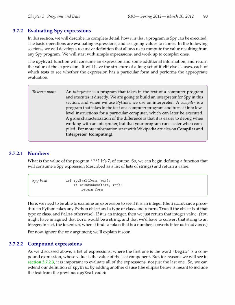
Chapter 3 Programs and Data 6.01— Spring 2012—March 10, 2012 90
3.7.2 Evaluating Spy expressionsIn this section, wewill describe, in complete detail, how it is that a program in Spy can be executed.The basic operations are evaluating expressions, and assigning values to names. In the followingsections, we will develop a recursive definition that allows us to compute the value resulting fromany Spy program. We will start with simple expressions, and work up to complex ones.
The spyEval function will consume an expression and some additional information, and returnthe value of the expression. It will have the structure of a long set of if-elif-else clauses, each ofwhich tests to see whether the expression has a particular form and performs the appropriateevaluation.
To learn more: An interpreter is a program that takes in the text of a computer programand executes it directly. We are going to build an interpreter for Spy in thissection, and when we use Python, we use an interpreter. A compiler is aprogram that takes in the text of a computer program and turns it into low-level instructions for a particular computer, which can later be executed.A gross characterization of the difference is that it is easier to debug whenworking with an interpreter, but that your program runs faster when com-piled. For more information start withWikipedia articles onCompiler andInterpreter_(computing).
3.7.2.1 NumbersWhat is the value of the program ’7’? It’s 7, of course. So, we can begin defining a function thatwill consume a Spy expression (described as a list of lists of strings) and return a value.
Spy Eval def spyEval(form, env):if isinstance(form, int):
return form
Here, we need to be able to examine an expression to see if it is an integer (the isinstance proce-dure in Python takes any Python object and a type or class, and returns True if the object is of thattype or class, and False otherwise). If it is an integer, then we just return that integer value. (Youmight have imagined that form would be a string, and that we’d have to convert that string to aninteger; in fact, the tokenizer, when it finds a token that is a number, converts it for us in advance.)
For now, ignore the env argument; we’ll explain it soon.
3.7.2.2 Compound expressionsAs we discussed above, a list of expressions, where the first one is the word ’begin’ is a com-pound expression, whose value is the value of the last component. But, for reasons we will see insection 3.7.2.3, it is important to evaluate all of the expressions, not just the last one. So, we canextend our definition of spyEval by adding another clause (the ellipsis below is meant to includethe text from the previous spyEval code):
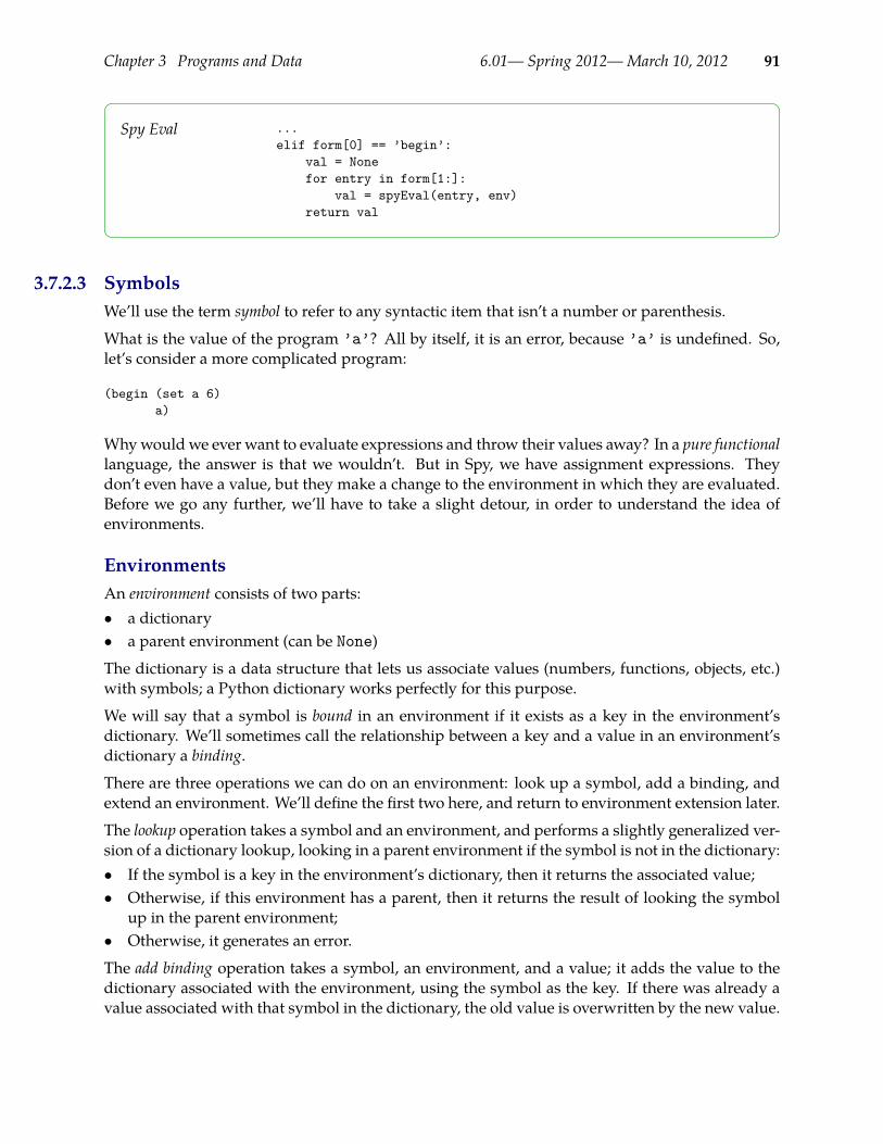
Chapter 3 Programs and Data 6.01— Spring 2012—March 10, 2012 91
Spy Eval ...elif form[0] == ’begin’:
val = Nonefor entry in form[1:]:
val = spyEval(entry, env)return val
3.7.2.3 SymbolsWe’ll use the term symbol to refer to any syntactic item that isn’t a number or parenthesis.
What is the value of the program ’a’? All by itself, it is an error, because ’a’ is undefined. So,let’s consider a more complicated program:
(begin (set a 6)a)
Whywouldwe ever want to evaluate expressions and throw their values away? In a pure functionallanguage, the answer is that we wouldn’t. But in Spy, we have assignment expressions. Theydon’t even have a value, but they make a change to the environment in which they are evaluated.Before we go any further, we’ll have to take a slight detour, in order to understand the idea ofenvironments.
EnvironmentsAn environment consists of two parts:• a dictionary• a parent environment (can be None)
The dictionary is a data structure that lets us associate values (numbers, functions, objects, etc.)with symbols; a Python dictionary works perfectly for this purpose.
We will say that a symbol is bound in an environment if it exists as a key in the environment’sdictionary. We’ll sometimes call the relationship between a key and a value in an environment’sdictionary a binding.
There are three operations we can do on an environment: look up a symbol, add a binding, andextend an environment. We’ll define the first two here, and return to environment extension later.
The lookup operation takes a symbol and an environment, and performs a slightly generalized ver-sion of a dictionary lookup, looking in a parent environment if the symbol is not in the dictionary:• If the symbol is a key in the environment’s dictionary, then it returns the associated value;• Otherwise, if this environment has a parent, then it returns the result of looking the symbol
up in the parent environment;• Otherwise, it generates an error.
The add binding operation takes a symbol, an environment, and a value; it adds the value to thedictionary associated with the environment, using the symbol as the key. If there was already avalue associated with that symbol in the dictionary, the old value is overwritten by the new value.

Chapter 3 Programs and Data 6.01— Spring 2012—March 10, 2012 92
’a’ 9
’c’ 12
’a’ 6
’b’ 7
Figure 3.1 A simple environment.
Exercise 3.19. If e is the environment in Figure 3.1, what are the results of:• e.lookup(’a’)• e.lookup(’c’)• e.lookup(’d’)• e.add(’f’, 1)• e.add(’c’, 2)• e.add(’a’, 2)
Where do environments come from? There is one environment that is made by the interpreter,called global. It contains bindings for the primitive procedures, and is the environment in whichour main program is evaluated.
Assigning valuesSo, let’s go back to the expression
(set a 6)
We’ll refer to the second and third elements of this expression (the ’a’ and the 6) as the left-hand-side (lhs) and right-hand-side (rhs) respectively.25 For now, the lhs will always be a symbol. Now,to evaluate this expression in an environment, we evaluate the expression that is the rhs to get avalue, and then bind the symbol that is the lhs to that value in the environment.
So, here’s our augmented definition of eval. Note that it we have added the env argument, whichis the environment in which we’re evaluating the expression:
Spy Eval elif form[0] == ’set’:(tag, lhs, rhs) = formenv.add(lhs, spyEval(rhs, env))
So, in our simple example, lhs is the symbol ’a’; expr is 6, which does not need further evaluation(the tokenizer has already turned the string ’6’) into an internal Python integer 6. More generally,though, the expr can be an arbitrarily complicated expression which might take a great deal ofwork to evaluate.
After we have evaluated that expression, our global environment will look like this:
That usage comes because a typical assignment statement has the form lhs = rhs.25
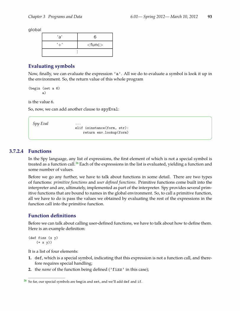
Chapter 3 Programs and Data 6.01— Spring 2012—March 10, 2012 93
’a’ 6
’+’ <func>...
global
Evaluating symbolsNow, finally, we can evaluate the expression ’a’. All we do to evaluate a symbol is look it up inthe environment. So, the return value of this whole program
(begin (set a 6)a)
is the value 6.
So, now, we can add another clause to spyEval:
Spy Eval ...elif isinstance(form, str):
return env.lookup(form)
3.7.2.4 FunctionsIn the Spy language, any list of expressions, the first element of which is not a special symbol istreated as a function call.26 Each of the expressions in the list is evaluated, yielding a function andsome number of values.
Before we go any further, we have to talk about functions in some detail. There are two typesof functions: primitive functions and user defined functions. Primitive functions come built into theinterpreter and are, ultimately, implemented as part of the interpreter. Spy provides several prim-itive functions that are bound to names in the global environment. So, to call a primitive function,all we have to do is pass the values we obtained by evaluating the rest of the expressions in thefunction call into the primitive function.
Function definitionsBefore we can talk about calling user-defined functions, we have to talk about how to define them.Here is an example definition:
(def fizz (x y)(+ x y))
It is a list of four elements:1. def, which is a special symbol, indicating that this expression is not a function call, and there-
fore requires special handling;2. the name of the function being defined (’fizz’ in this case);
So far, our special symbols are begin and set, and we’ll add def and if.26
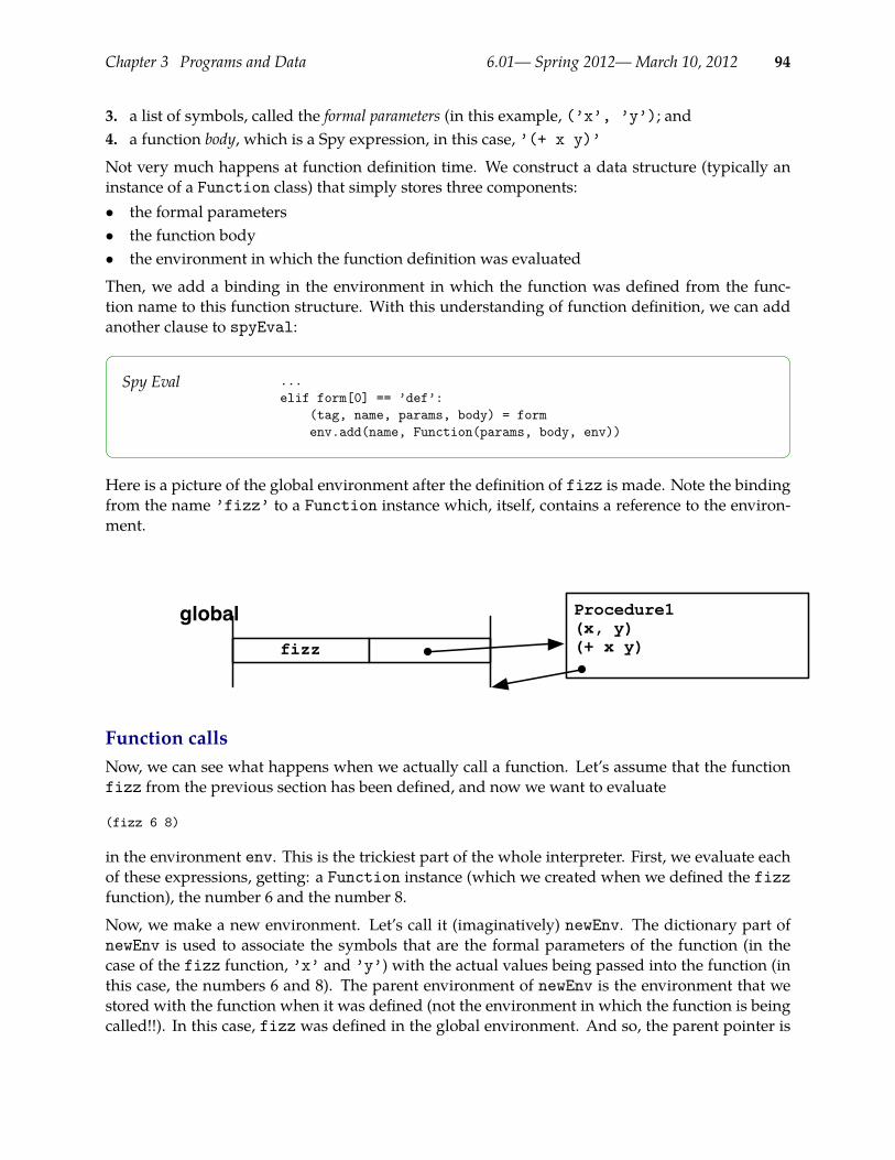
Chapter 3 Programs and Data 6.01— Spring 2012—March 10, 2012 94
3. a list of symbols, called the formal parameters (in this example, (’x’, ’y’); and4. a function body, which is a Spy expression, in this case, ’(+ x y)’
Not very much happens at function definition time. We construct a data structure (typically aninstance of a Function class) that simply stores three components:• the formal parameters• the function body• the environment in which the function definition was evaluated
Then, we add a binding in the environment in which the function was defined from the func-tion name to this function structure. With this understanding of function definition, we can addanother clause to spyEval:
Spy Eval ...elif form[0] == ’def’:
(tag, name, params, body) = formenv.add(name, Function(params, body, env))
Here is a picture of the global environment after the definition of fizz is made. Note the bindingfrom the name ’fizz’ to a Function instance which, itself, contains a reference to the environ-ment.
fizz
global Procedure1(x, y)(+ x y)
Function callsNow, we can see what happens when we actually call a function. Let’s assume that the functionfizz from the previous section has been defined, and now we want to evaluate
(fizz 6 8)
in the environment env. This is the trickiest part of the whole interpreter. First, we evaluate eachof these expressions, getting: a Function instance (which we created when we defined the fizzfunction), the number 6 and the number 8.
Now, we make a new environment. Let’s call it (imaginatively) newEnv. The dictionary part ofnewEnv is used to associate the symbols that are the formal parameters of the function (in thecase of the fizz function, ’x’ and ’y’) with the actual values being passed into the function (inthis case, the numbers 6 and 8). The parent environment of newEnv is the environment that westored with the function when it was defined (not the environment in which the function is beingcalled!!). In this case, fizz was defined in the global environment. And so, the parent pointer is
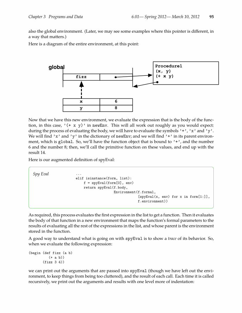
Chapter 3 Programs and Data 6.01— Spring 2012—March 10, 2012 95
also the global environment. (Later, we may see some examples where this pointer is different, ina way that matters.)Here is a diagram of the entire environment, at this point:
fizz
global Procedure1(x, y)(+ x y)
y 8x 6
Now that we have this new environment, we evaluate the expression that is the body of the func-tion, in this case, ’(+ x y)’ in newEnv. This will all work out roughly as you would expect:during the process of evaluating the body, we will have to evaluate the symbols ’+’, ’x’ and ’y’.We will find ’x’ and ’y’ in the dictionary of newEnv; and we will find ’+’ in its parent environ-ment, which is global. So, we’ll have the function object that is bound to ’+’, and the number6 and the number 8; then, we’ll call the primitive function on these values, and end up with theresult 14.Here is our augmented definition of spyEval:
Spy Eval ...elif isinstance(form, list):
f = spyEval(form[0], env)return spyEval(f.body,
Environment(f.formal,[spyEval(x, env) for x in form[1:]],f.environment))
As required, this process evaluates the first expression in the list to get a function. Then it evaluatesthe body of that function in a new environment that maps the function’s formal parameters to theresults of evaluating all the rest of the expressions in the list, and whose parent is the environmentstored in the function.A good way to understand what is going on with spyEval is to show a trace of its behavior. So,when we evaluate the following expression:
(begin (def fizz (a b)(+ a b))
(fizz 3 4))
we can print out the arguments that are passed into spyEval (though we have left out the envi-ronment, to keep things from being too cluttered), and the result of each call. Each time it is calledrecursively, we print out the arguments and results with one level more of indentation:
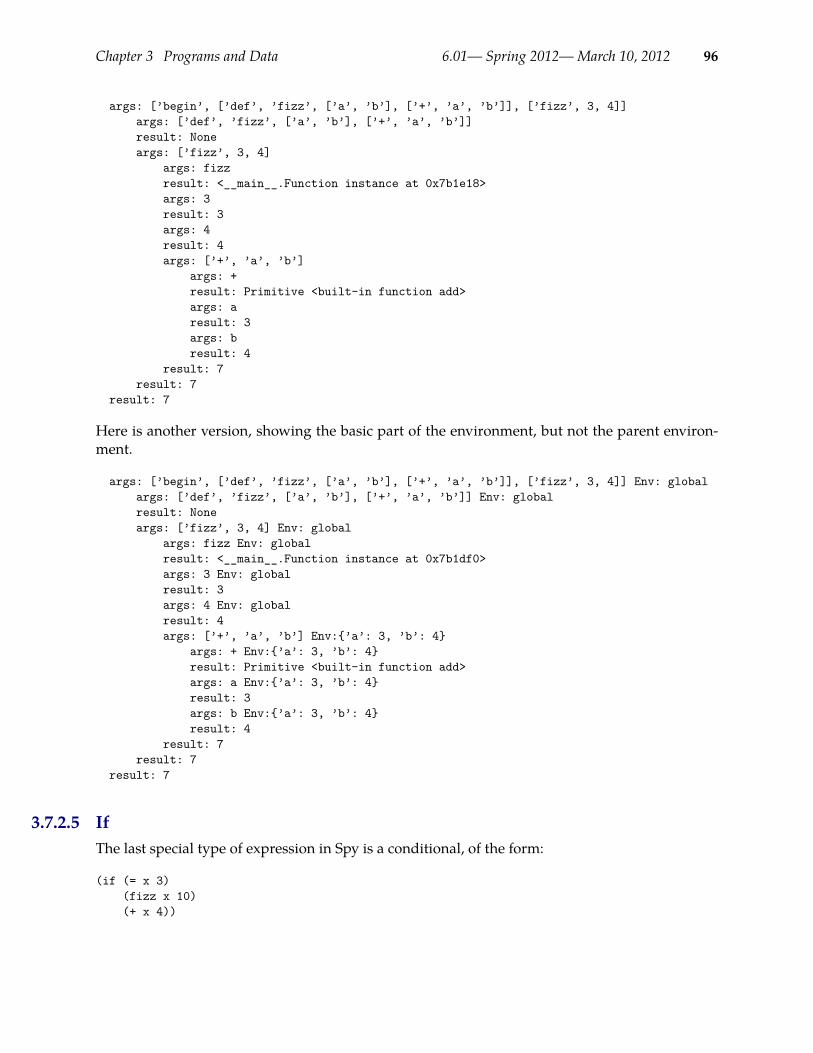
Chapter 3 Programs and Data 6.01— Spring 2012—March 10, 2012 96
args: [’begin’, [’def’, ’fizz’, [’a’, ’b’], [’+’, ’a’, ’b’]], [’fizz’, 3, 4]]args: [’def’, ’fizz’, [’a’, ’b’], [’+’, ’a’, ’b’]]result: Noneargs: [’fizz’, 3, 4]
args: fizzresult: <__main__.Function instance at 0x7b1e18>args: 3result: 3args: 4result: 4args: [’+’, ’a’, ’b’]
args: +result: Primitive <built-in function add>args: aresult: 3args: bresult: 4
result: 7result: 7
result: 7
Here is another version, showing the basic part of the environment, but not the parent environ-ment.
args: [’begin’, [’def’, ’fizz’, [’a’, ’b’], [’+’, ’a’, ’b’]], [’fizz’, 3, 4]] Env: globalargs: [’def’, ’fizz’, [’a’, ’b’], [’+’, ’a’, ’b’]] Env: globalresult: Noneargs: [’fizz’, 3, 4] Env: global
args: fizz Env: globalresult: <__main__.Function instance at 0x7b1df0>args: 3 Env: globalresult: 3args: 4 Env: globalresult: 4args: [’+’, ’a’, ’b’] Env:’a’: 3, ’b’: 4
args: + Env:’a’: 3, ’b’: 4result: Primitive <built-in function add>args: a Env:’a’: 3, ’b’: 4result: 3args: b Env:’a’: 3, ’b’: 4result: 4
result: 7result: 7
result: 7
3.7.2.5 IfThe last special type of expression in Spy is a conditional, of the form:
(if (= x 3)(fizz x 10)(+ x 4))
Chapter 3 Programs and Data 6.01— Spring 2012—March 10, 2012 97
It might seem, at first, that it would be okay to implement if as a primitive function, similar to +.But there is an important reason not to do so. Consider the definition of the factorial function, inSpy:
(def factorial (x)(if (= x 1)
1(* x (factorial (- x 1)))))
The most straightforward application of this function, (factorial 1) will get us into trouble.Why? We would start by evaluating ’factorial’ and ’1’, and getting a function and 1. So farso good. Now we make a new environment, and evaluate the body in that environment. Thatrequires evaluating all of the elements of the body in that environment. So, we’d find that ’if’evaluates to a primitive function, that (= x 1) evaluates to True, and that 1 evaluates to 1. Then,we’d need to evaluate that last expression, which is itself a function call. That, in itself, is noproblem. But we can see that eventually, we’ll have to evaluate factorial in an environment whereits argument is -1. And that will require evaluating factorial of -2, which will require evaluatingfactorial of -3, and so on.
Themost important thing about ’if’ is that it evaluates only one of its branches, depending on whetherits condition is True or False. Without this property, we cannot stop recursion.
So, now we can see what to do with an ’if’ expression. We’ll call the second, third, and fourthelements the condition, then and else parts. We start by evaluating the condition part. If it is True,we evaluate the then part, otherwise we evaluate the else part.
It is pretty straightforward to add this to our eval function; but note that we had to put it beforethe function application clause, so that we can keep if expressions from being evaluated as if theywere function applications.
Here is the whole interpreter.

Chapter 3 Programs and Data 6.01— Spring 2012—March 10, 2012 98
Spy Eval def spyEval(form, env=globalEnv):if isinstance(form, int):
return formelif isinstance(form, str):
return env.lookup(form)elif form[0] == ’begin’:
val = Nonefor entry in form[1:]:
val = spyEval(entry, env)return val
elif form[0] == ’set’:(tag, lhs, rhs) = formenv.add(lhs, spyEval(rhs, env))
elif form[0] == ’def’:(tag, name, params, body) = formenv.add(name, Function(params, body, env))
elif form[0] == ’if’:(tag, condition, ifBody, elseBody) = formif spyEval(condition, env)
return spyEval(ifBody, env)else:
return spyEval(elseBody, env)elif isinstance(form, list):
f = spyEval(form[0], env)return spyEval(f.body,
Environment(f.formal,[spyEval(x, env) for x in form[1:]],f.environment))
else:Error("Illegal expression: "+str(form))
Yay! Now we have a complete Spy interpreter. Well, we still need implementations of the Envi-ronment and Function classes, but that’s not very much more work. We can implement thoseclasses as exercises.
3.7.3 Object-Oriented SpyWe can add a simple object-oriented facility to Spy, which is modeled on Python’s OOP facility,but is somewhat simpler. The crucial idea here is that classes and instances are both environments, ofexactly the same kind that we have been using to support binding and function calls in basic Spy.The dictionary part of the environment supports the binding of attribute names to values withinthe instance or class; and the parent environment part allows an instance to be connected to itsclass, or a class to its superclass, so that attributes that are not defined within the instance may befound in the class or superclass.We only have to add two new syntactic features to the language: attribute lookup and class defi-nition.
3.7.3.1 Attribute lookupIn Python, when you want to get the value of an attribute a from an instance obj, you say obj.a.In OOSpy, we’ll say (attr obj a). Remembering that an instance is an environment, all we haveto do to evaluate such an expression is to look up the symbol ’a’ in the environment ’obj’.

Chapter 3 Programs and Data 6.01— Spring 2012—March 10, 2012 99
Referring to the second part of this form as the object part and the third as the name part, we canadd a clause for attr expressions to our interpreter. The name will always be a single symbol;but the object part can be a general expression (we might, for example, call a function bigFun thatreturns an object, yielding an expression like (attr (bigFun 3) x) to get the attribute namedx from the object returned by bigFun). This means that we have to evaluate the object part, usingour standard evaluation function. Now, we can add a clause for attr expressions to our spyEval:
Spy Eval ...elif form[0] == ’attr’:
(tag, objectExpr, name) = formreturn spyEval(objectExpr, env).lookup(name)
...
3.7.3.2 Class definitionAll the rest of our work happens at class definition time. Here is a simple OOSpy class definition:
(class SimpleClass None(begin (def init (self v)
(set (attr self v) v))(def getV (self)
(attr self v))))
For reference, it is roughly equivalent to the Python:
class SimpleClass:def init (self, v):
self.v = vdef getV (self):
return self.v
It has four parts: the special symbol ’class’, the class name SimpleClass, the name of a su-perclass (in this case, there is no superclass, so we write None), and a class body, which is a Spyexpression. Our simple Spy implementation doesn’t have an equivalent to Python’s __init__ fa-cility, in which the specially-named procedure is called automatically. So we call the method initwithout underscores to make that clear.
Here is a picture of the environment that we would like to have result from this definition:
SimpleClass
globalinitgetV
Procedure1()return Environment( )
Procedure3(self)return self.v
Procedure2(self,v)self.v = v

Chapter 3 Programs and Data 6.01— Spring 2012—March 10, 2012 100
Note that Spy differs from Python here in an important way: in Python, the environment storedin a method is always the module environment; in Spy, to avoid having a special case, it is theclass environment in which it is defined.
Also, rather than binding SimpleClass directly to the environment for the class, wewill bind it toa procedure thatmakes a new environmentwhose parent is the class environment. This procedurecan be called directly to create a new instance of the class.
There are three steps involved in processing this class definition.1. Make an environment for the class In this step, we just make a new empty environment, and
set its parent to be the class specified as the superclass of this class. If the superclass is None,then we use global as the parent environment, so that global variables and primitive functiondefinitions will be accessible from the class body.
2. Evaluate the class body in the class environment In this step, we use our regular Spy evaluationmechanism, to evaluate the class body, in the new environment. In our SimpleClass body,we define two methods; these definitions will appear in the class environment but will not, forexample, be accessible directly from the global environment.
3. Make a constructor function Finally, we define a new function, with the same name as the class,in the environment in which the class definition is being evaluated (not the class environment;if we did that, nobody would every be able to find the constructor!). The constructor functionhas the job of making a new instance of this class. What is an instance? An environment. Anda brand new instance of any class is simply an empty environment, whose parent environmentis the class environment.
After defining SimpleClass, we can use it as follows:
(begin(set a (SimpleClass))((attr a init) a 37)((attr a getV) a))
This is roughly equivalent to the Python
a = SimpleClass()a.init(37)a.getV()
This may look a little bit strange. Let’s go step by step. First, we make an instance by calling theconstructor function. That’s pretty straightforward. Now, the value of variable a is an instance ofthe SimpleClass class, which means that it is an environment.
Now, what about this expression?
((attr a init) a 37)
Let’s try to work through it the way the interpreter would. It is a list, and the first element is not aspecial symbol, so it must be a function call. That means we should evaluate each of the forms inthe list.
First we evaluate (attr a init), which is a list starting with the special symbol attr, so weknow it’s looking up an attribute in a class. It evaluates the expression a, getting the SimpleClass
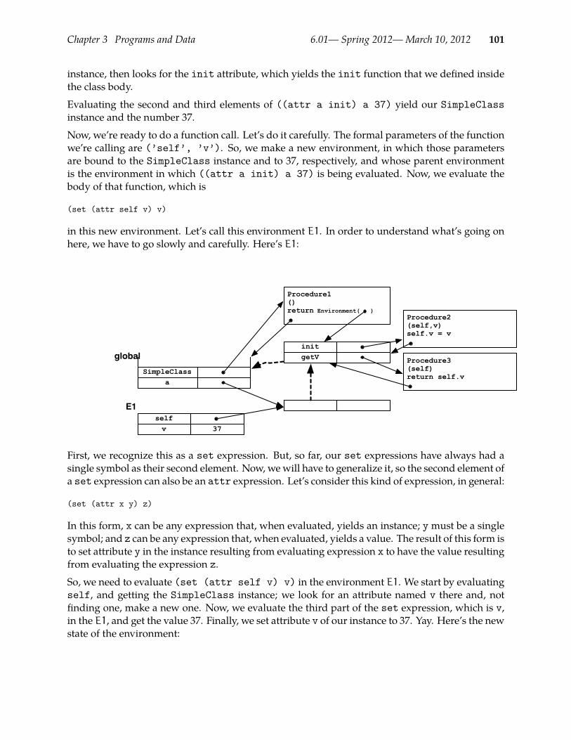
Chapter 3 Programs and Data 6.01— Spring 2012—March 10, 2012 101
instance, then looks for the init attribute, which yields the init function that we defined insidethe class body.
Evaluating the second and third elements of ((attr a init) a 37) yield our SimpleClassinstance and the number 37.
Now, we’re ready to do a function call. Let’s do it carefully. The formal parameters of the functionwe’re calling are (’self’, ’v’). So, we make a new environment, in which those parametersare bound to the SimpleClass instance and to 37, respectively, and whose parent environmentis the environment in which ((attr a init) a 37) is being evaluated. Now, we evaluate thebody of that function, which is
(set (attr self v) v)
in this new environment. Let’s call this environment E1. In order to understand what’s going onhere, we have to go slowly and carefully. Here’s E1:
aSimpleClass
globalinitgetV
Procedure1()return Environment( )
Procedure3(self)return self.v
Procedure2(self,v)self.v = v
37vself
E1
First, we recognize this as a set expression. But, so far, our set expressions have always had asingle symbol as their second element. Now, wewill have to generalize it, so the second element ofa set expression can also be an attr expression. Let’s consider this kind of expression, in general:
(set (attr x y) z)
In this form, x can be any expression that, when evaluated, yields an instance; ymust be a singlesymbol; and z can be any expression that, when evaluated, yields a value. The result of this form isto set attribute y in the instance resulting from evaluating expression x to have the value resultingfrom evaluating the expression z.
So, we need to evaluate (set (attr self v) v) in the environment E1. We start by evaluatingself, and getting the SimpleClass instance; we look for an attribute named v there and, notfinding one, make a new one. Now, we evaluate the third part of the set expression, which is v,in the E1, and get the value 37. Finally, we set attribute v of our instance to 37. Yay. Here’s the newstate of the environment:

Chapter 3 Programs and Data 6.01— Spring 2012—March 10, 2012 102
aSimpleClass
globalinitgetV
Procedure1()return Environment( )
Procedure3(self)return self.v
Procedure2(self,v)self.v = v
37vself
E1
One thing to notice is that Spy, as we have designed it, doesn’t have Python’s special facility thatautomatically uses an object as the first argument of a method, when that method is accessed viathat object. So, we have to pass the object in again, explicitly, as the first argument.
Exercise 3.20.Add this syntactic facility to OOSpy.That is, make it so that we can write ((attr a init) 37) and ((attr agetV)). This is a little bit tricky.
Evaluating the expression ((attr a getV) a) works similarly (you should be sure you under-stand how), and returns the value 37.
So, after all that, we can add the last clause to ourOOSpy interpreter, for handling class definitions.Note that we also have to extend the code for handling set, so it can deal with setting attributesof instances.
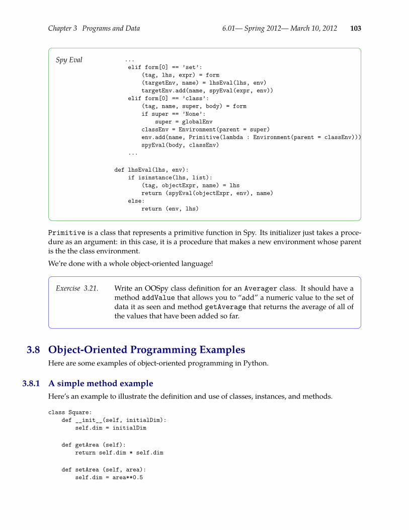
Chapter 3 Programs and Data 6.01— Spring 2012—March 10, 2012 103
Spy Eval ...elif form[0] == ’set’:
(tag, lhs, expr) = form(targetEnv, name) = lhsEval(lhs, env)targetEnv.add(name, spyEval(expr, env))
elif form[0] == ’class’:(tag, name, super, body) = formif super == ’None’:
super = globalEnvclassEnv = Environment(parent = super)env.add(name, Primitive(lambda : Environment(parent = classEnv)))spyEval(body, classEnv)
...
def lhsEval(lhs, env):if isinstance(lhs, list):
(tag, objectExpr, name) = lhsreturn (spyEval(objectExpr, env), name)
else:return (env, lhs)
Primitive is a class that represents a primitive function in Spy. Its initializer just takes a proce-dure as an argument: in this case, it is a procedure that makes a new environment whose parentis the the class environment.
We’re done with a whole object-oriented language!
Exercise 3.21. Write an OOSpy class definition for an Averager class. It should have amethod addValue that allows you to “add” a numeric value to the set ofdata it as seen and method getAverage that returns the average of all ofthe values that have been added so far.
3.8 Object-Oriented Programming ExamplesHere are some examples of object-oriented programming in Python.
3.8.1 A simple method exampleHere’s an example to illustrate the definition and use of classes, instances, and methods.
class Square:def __init__(self, initialDim):
self.dim = initialDim
def getArea (self):return self.dim * self.dim
def setArea (self, area):self.dim = area**0.5

Chapter 3 Programs and Data 6.01— Spring 2012—March 10, 2012 104
def __str__(self):return "Square of dim " + str(self.dim)
This class is meant to represent a square. Squares need to store, or remember, their dimension,so we make an attribute for it, and assign it in the __init__ method. Now, we define a methodgetArea that is intended to return the area of the square. There are a couple of interesting thingsgoing on here.
Like all methods, getArea has an argument, self, which will stand for the instance that thismethod is supposed to operate on. Now, the way we can find the dimension of the square is byfinding the value of the dim attribute of self.
We define another method, setArea, which will set the area of the square to a given value. Inorder to change the square’s area, we have to compute a new dimension and store it in the dimattribute of the square instance.27
Now, we can experiment with instances of class Square.
>>> s = Square(6)>>> s.getArea()36>>> Square.getArea(s)36>>> s.dim6>>> s.setArea(100)>>> s.dim10.0>>> s1 = Square(10)>>> s1.dim10>>> s1.getArea()100>>> s2 = Square(100)>>> s2.getArea()10000>>> print s1Square of dim 10
Our class Square has the __str__method defined, so it prints out nicely.
3.8.2 Superclasses and inheritanceWhat if we wanted to make a set of classes and instances that would help us to run a bank? Wecould start like this:
class Account:def __init__(self, initialBalance):
self.currentBalance = initialBalancedef balance(self):
return self.currentBalancedef deposit(self, amount):
self.currentBalance = self.currentBalance + amount
We compute the square root of a value by raising to the power 0.5.27

Chapter 3 Programs and Data 6.01— Spring 2012—March 10, 2012 105
def creditLimit(self):return min(self.currentBalance * 0.5, 10000000)
>>> a = Account(100)>>> b = Account(1000000)
>>> Account.balance(a)100>>> a.balance()100>>> Account.deposit(a, 100)>>> a.deposit(100)>>> a.balance()300>>> b.balance()1000000
We’ve made an Account class28 that maintains a balance as an attribute. There are methods forreturning the balance, for making a deposit, and for returning the credit limit.
The Account class contains the procedures that are common to all bank accounts; the individualinstances contain state in the values associated with the names in their environments. That stateis persistent, in the sense that it exists for the lifetime of the program that is running, and doesn’tdisappear when a particular method call is over.
Now, imagine that the bank we’re running is getting bigger, and we want to have several differentkinds of accounts, with the credit limit depending on the account type. If we wanted to defineanother type of account as a Python class, we could do it this way:
class PremierAccount:def __init__(self, initialBalance):
self.currentBalance = initialBalancedef balance(self):
return self.currentBalancedef deposit(self, amount):
self.currentBalance = self.currentBalance + amountdef creditLimit(self):
return min(self.currentBalance * 1.5, 10000000)>>> c = PremierAccount(1000)>>> c.creditLimit()1500.0
This will let people with premier accounts have larger credit limits. And, the nice thing is that wecan ask for its credit limit without knowing what kind of an account it is, so we see that objectssupport generic functions, which operate on different kinds of objects by doing different, but type-appropriate operations.
A note on style. It is useful to adopt some conventions for naming things, just to help your programs be more read-28
able. We’ve used the convention that variables and procedure names start with lower case letters and that classnames start with upper case letters. And we try to be consistent about using something called “camel caps” forwriting compound words, which is to write a compound name with the successiveWordsCapitalized. An alternativeis_to_use_underscores.

Chapter 3 Programs and Data 6.01— Spring 2012—March 10, 2012 106
However, this solution is still not satisfactory. In order to make a premier account, we had torepeat a lot of the definitions from the basic account class, violating our fundamental principle oflaziness: never do twice what you could do once; instead, abstract and reuse.
Inheritance lets us make a new class that’s like an old class, but with some parts overridden or newparts added. When defining a class, you can actually specify an argument, which is another class.You are saying that this new class should be exactly like the parent class or superclass, but withcertain definitions added or overridden. So, for example, we can say
class PremierAccount(Account):def creditLimit(self):
return min(self.currentBalance * 1.5, 10000000)
class EconomyAccount(Account):def creditLimit(self):
return min(self.currentBalance*0.5, 20.00)
>>> a = Account(100)>>> b = PremierAccount(100)>>> c = EconomyAccount(100)>>> a.creditLimit()100.0>>> b.creditLimit()150.0>>> c.creditLimit()20.0
We automatically inherit the methods of our superclass (including __init__). So we still knowhow to make deposits into a premier account:
>>> b.deposit(100)>>> b.balance()200
The fact that instances know what class they were derived from allows us to ask each instanceto do the operations appropriate to it, without having to take specific notice of what class it is.Procedures that can operate on instances of different types or classeswithout explicitly taking theirtypes or classes into account are called polymorphic. Polymorphism is a very powerful method forcapturing common patterns.
3.8.3 A data type for timesObject-oriented programming is particularly useful when we want to define a new compositionaldata type: that is, a representation for the data defining a class of objects and one or more oper-ations for creating new instances of the class from old instances. We might do this with complexnumbers or points in a high-dimensional space.
Here we demonstrate the basic ideas with a very simple class for representing times.
We’ll start by defining an initialization method, with default values specified for the parameters.
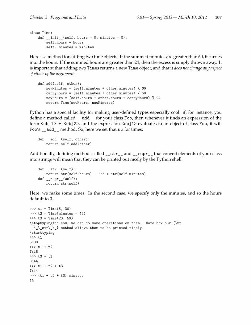
Chapter 3 Programs and Data 6.01— Spring 2012—March 10, 2012 107
class Time:def __init__(self, hours = 0, minutes = 0):
self.hours = hoursself. minutes = minutes
Here is amethod for adding two time objects. If the summedminutes are greater than 60, it carriesinto the hours. If the summed hours are greater than 24, then the excess is simply thrown away. Itis important that adding two Times returns a new Time object, and that it does not change any aspectof either of the arguments.
def add(self, other):newMinutes = (self.minutes + other.minutes) % 60carryHours = (self.minutes + other.minutes) / 60newHours = (self.hours + other.hours + carryHours) % 24return Time(newHours, newMinutes)
Python has a special facility for making user-defined types especially cool: if, for instance, youdefine a method called __add__ for your class Foo, then whenever it finds an expression of theform <obj1> + <obj2>, and the expression <obj1> evaluates to an object of class Foo, it willFoo’s __add__method. So, here we set that up for times:
def __add__(self, other):return self.add(other)
Additionally, defining methods called __str__ and __repr__ that convert elements of your classinto strings will mean that they can be printed out nicely by the Python shell.
def __str__(self):return str(self.hours) + ’:’ + str(self.minutes)
def __repr__(self):return str(self)
Here, we make some times. In the second case, we specify only the minutes, and so the hoursdefault to 0.
>>> t1 = Time(6, 30)>>> t2 = Time(minutes = 45)>>> t3 = Time(23, 59)\stoptypingAnd now, we can do some operations on them. Note how our \tt\_\_str\_\_ method allows them to be printed nicely.
\starttyping>>> t16:30>>> t1 + t27:15>>> t3 + t20:44>>> t1 + t2 + t37:14>>> (t1 + t2 + t3).minutes14

Chapter 3 Programs and Data 6.01— Spring 2012—March 10, 2012 108
3.8.4 Practice problem: argmaxWrite a Python procedure argmax that takes two arguments: the first is a list of elements, and thesecond is a function from elements to numerical values. It should return the element of the listwith the highest numerical score.
def argmax(elements, f):bestScore = NonebestElement = Nonefor e in elements:
score = f(e)if bestScore == None or score > bestScore:
bestScore = scorebestElement = e
return bestElement
def argmax(elements, f):bestElement = elements[0]for e in elements:
if f(e) > f(bestElement):bestElement = e
return bestElement
def argmax(elements, f):vals = [f(e) for e in elements]return elements[vals.index(max(vals))]
def argmax(elements, f):return max(elements, key=f)
There are many ways of writing this. Here are a few. It’s important to keep straight in yourhead which variables contain scores and which contain elements. Any of these solutionswould have been fine; we wouldn’t expect most people to get the last one.
3.8.5 Practice problem: OOPThe following definitions have been entered into a Python shell:
class A:yours = 0def __init__(self, inp):
self.yours = inpdef give(self, amt):
self.yours = self.yours + amtreturn self.yours
def howmuch(self):return (A.yours, self.yours)
class B(A):yours = 0def give(self, amt):
B.yours = B.yours + amtreturn A.howmuch(self)

Chapter 3 Programs and Data 6.01— Spring 2012—March 10, 2012 109
def take(self, amt):self.yours = self.yours - amtreturn self.yours
def howmuch(self):return (B.yours, A.yours, self.yours)
Write the values of the following expressions. Write None when there is no value; write Errorwhen an error results and explain briefly why it is an error. Assume that these expressions areevaluated one after another (all of the left column first, then right column).
test = A(5)
test.take(2)
test.give(6)
test.howmuch()
test = B(5)
test.take(2)
test.give(6)
test.howmuch()
• None: This makes test be equal to a new instance of A, with attribute yours equal to 5.• Error: Instances of A don’t have a takemethod.• 11: This adds 6 to the value of test.yours and returns its value.• (0, 11): At this point, we haven’t changed the class attribute A.yours, so it still has value
0.• None: This makes test be equal to a new instance of B; it inherits the init method from A,
so at this point test.yours is equal to 5.• 3: Now, since test is an instance of B, the method test.take is defined; it changes
test.yours to be 3 and returns its value.• (0, 3): Note that this refers to the givemethod defined in class B. So, first, the amount is
used to increment B.yours to have value 6. Then, we return A.yours and test.yours,which are both unchanged.
• (6, 0, 3): This just returns the current values of all three yours attributes, one in eachclass definition as well as test.yours.
3.8.6 Practice problem: The Best and the BrightestHere are some class definitions, meant to represent a collection of students making up the studentbody of a prestigious university.
class Student:def __init__(self, name, iq, salary, height):
self.name = nameself.iq = iqself.salary = salaryself.height = height
class StudentBody:def __init__(self):
self.students = []def addStudent(self, student):
self.students.append(student)

Chapter 3 Programs and Data 6.01— Spring 2012—March 10, 2012 110
def nameOfSmartest(self):# code will go here
def funOfBest(self, fun, feature):# code will go here
The StudentBody class is missing the code for two methods:• nameOfSmartest: returns the name attribute of the student with the highest IQ• funOfBest: takes a procedure fun and a procedure feature as input, and returns the result
of applying procedure fun to the student for whom the procedure feature yields the highestvalue
For the first two problems below, assume that these methods have been implemented.
Here is a student body:
jody = Student(’Jody’, 100, 100000, 80)chris = Student(’Chris’, 150, 40000, 62)dana = Student(’Dana’, 120, 2000, 70)aardvarkU = StudentBody()aardvarkU.addStudent(jody)aardvarkU.addStudent(chris)aardvarkU.addStudent(dana)
1. What is the result of evaluating aardvarkU.nameOfSmartest()?
’Chris’
2. Write a Python expression that will compute the name of the person who has the greatestvalue of IQ + height in aardvarkU (not just for the example student body above). You candefine additional procedures if you need them.
aardvarkU.funOfBest(lambda x: x.name, lambda x: x.iq + x.height)
The second lambda expression specifies how to evaluate an element (that is, to sum its iqand height attributes) and the first lambda expression says what function to apply to theelement with the highest score.
3. Implement the nameOfSmartest method. For full credit, use util.argmax (defined below)or the funOfBestmethod.
If l is a list of items and f is a procedure that maps an item into a numeric score, thenutil.argmax(l, f) returns the element of l that has the highest score.

Chapter 3 Programs and Data 6.01— Spring 2012—March 10, 2012 111
def nameOfSmartest(self):return util.argmax(self.students, lambda x: x.iq).name
# or
def nameOfSmartest(self):return funOfBest(lambda x: x.name, lambda x: x.iq)
Note that in the first solution, the expression util.argmax(self.students, lambda x:x.iq) returns the object with the highest iq attribute; then we return the name attribute ofthat object.
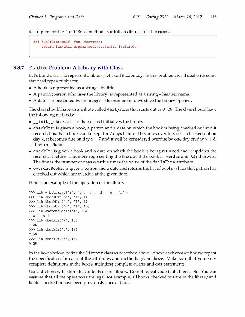
Chapter 3 Programs and Data 6.01— Spring 2012—March 10, 2012 112
4. Implement the funOfBestmethod. For full credit, use util.argmax.
def funOfBest(self, fun, feature):return fun(util.argmax(self.students, feature))
3.8.7 Practice Problem: A Library with ClassLet’s build a class to represent a library; let’s call it Library. In this problem, we’ll deal with somestandard types of objects:• A book is represented as a string – its title.• A patron (person who uses the library) is represented as a string – his/her name.• A date is represented by an integer – the number of days since the library opened.
The class should have an attribute called dailyFine that starts out as 0.25. The class should havethe following methods:• __init__: takes a list of books and initializes the library.• checkOut: is given a book, a patron and a date on which the book is being checked out and itrecords this. Each book can be kept for 7 days before it becomes overdue, i.e. if checked out onday x, it becomes due on day x + 7 and it will be considered overdue by one day on day x + 8.It returns None.• checkIn: is given a book and a date on which the book is being returned and it updates therecords. It returns a number representing the fine due if the book is overdue and 0.0 otherwise.The fine is the number of days overdue times the value of the dailyFine attribute.• overdueBooks: is given a patron and a date and returns the list of books which that patron haschecked out which are overdue at the given date.
Here is an example of the operation of the library:
>>> lib = Library([’a’, ’b’, ’c’, ’d’, ’e’, ’f’])>>> lib.checkOut(’a’, ’T’, 1)>>> lib.checkOut(’c’, ’T’, 1)>>> lib.checkOut(’e’, ’T’, 10)>>> lib.overdueBooks(’T’, 13)[’a’, ’c’]>>> lib.checkIn(’a’, 13)1.25>>> lib.checkIn(’c’, 18)2.50>>> lib.checkIn(’e’, 18)0.25
In the boxes below, define the Library class as described above. Above each answer boxwe repeatthe specification for each of the attributes and methods given above. Make sure that you entercomplete definitions in the boxes, including complete class and def statements.
Use a dictionary to store the contents of the library. Do not repeat code if at all possible. You canassume that all the operations are legal, for example, all books checked out are in the library andbooks checked in have been previously checked out.

Chapter 3 Programs and Data 6.01— Spring 2012—March 10, 2012 113
Class definition:
Include both the start of the class definition and the method definition for __init__ in this firstanswer box.
The class should have an attribute called dailyFine that starts out as 0.25.
__init__: takes a list of books and initializes the library.
class Library:dailyFine = 0.25def __init__(self, books):
self.shelf = for book in books:
self.shelf[book] = (None, None) # (patron, dueDate)
The crucial part here is deciding what information to store. Here, for each book, we store atuple of who has checked it out, and when it is due.
checkOut: is given a book, a patron and a date on which the book is being checked out and itrecords this. Each book can be kept for 7 days before it becomes overdue, i.e. if checked out onday x, it becomes due on day x + 7 and it will be considered overdue by one day on day x + 8. Itreturns None.
def checkOut(self, book, patron, date):self.shelf[book] = (patron, date+7)
checkIn: is given a book and a date on which the book is being returned and it updates therecords. It returns a number representing the fine due if the book is overdue and 0.0 otherwise.The fine is the number of days overdue times the value of the dailyFine attribute.
def checkIn(self, book, date):patron, due = self.shelf[book]self.shelf[book] = (None, None)return max(0.0, (date - due))*self.dailyFine
Note the destructuring assignment in the first line. It’s not crucial, but it’s nice style, andkeeps us from having to refer to components like self.shelf[book][1], which are ugly,long, and hard to get right. Instead of using a max, you could use an if statement to handlethe case of the book being overdue or not, but this is more compact and pretty clear.
overdueBooks: is given a patron and a date and returns the list of books which that patron haschecked out which are overdue at the given date.
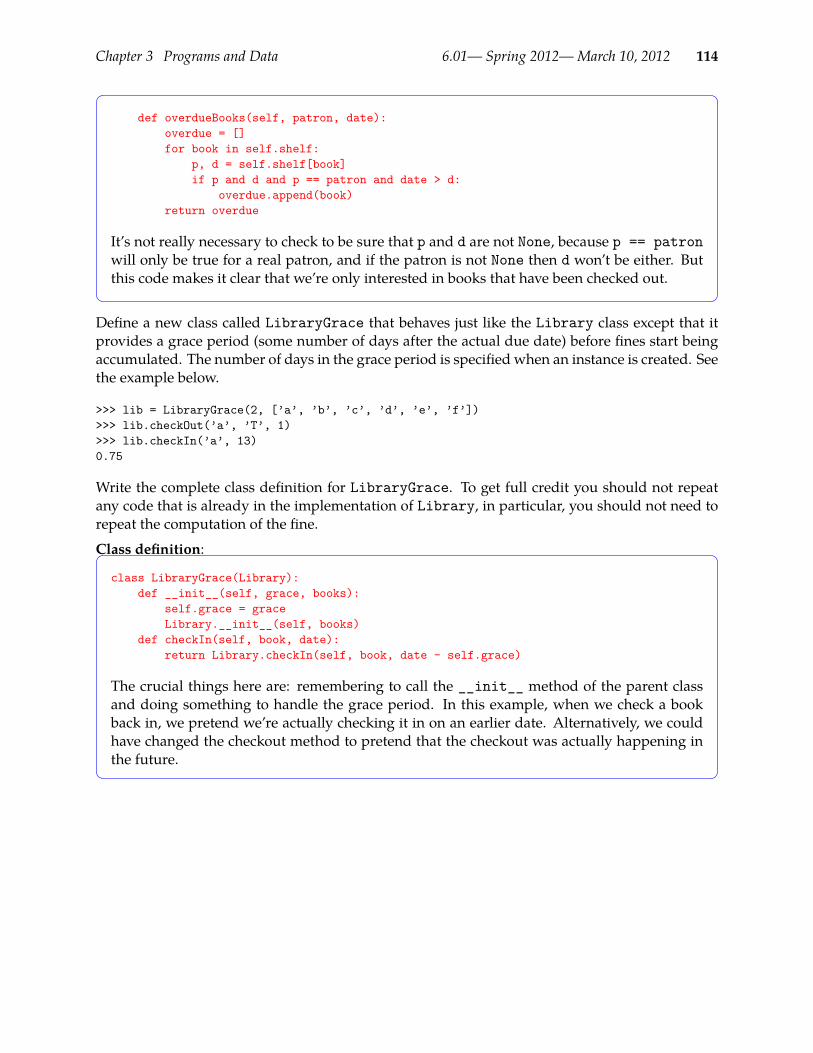
Chapter 3 Programs and Data 6.01— Spring 2012—March 10, 2012 114
def overdueBooks(self, patron, date):overdue = []for book in self.shelf:
p, d = self.shelf[book]if p and d and p == patron and date > d:
overdue.append(book)return overdue
It’s not really necessary to check to be sure that p and d are not None, because p == patronwill only be true for a real patron, and if the patron is not None then d won’t be either. Butthis code makes it clear that we’re only interested in books that have been checked out.
Define a new class called LibraryGrace that behaves just like the Library class except that itprovides a grace period (some number of days after the actual due date) before fines start beingaccumulated. The number of days in the grace period is specified when an instance is created. Seethe example below.
>>> lib = LibraryGrace(2, [’a’, ’b’, ’c’, ’d’, ’e’, ’f’])>>> lib.checkOut(’a’, ’T’, 1)>>> lib.checkIn(’a’, 13)0.75
Write the complete class definition for LibraryGrace. To get full credit you should not repeatany code that is already in the implementation of Library, in particular, you should not need torepeat the computation of the fine.
Class definition:
class LibraryGrace(Library):def __init__(self, grace, books):
self.grace = graceLibrary.__init__(self, books)
def checkIn(self, book, date):return Library.checkIn(self, book, date - self.grace)
The crucial things here are: remembering to call the __init__ method of the parent classand doing something to handle the grace period. In this example, when we check a bookback in, we pretend we’re actually checking it in on an earlier date. Alternatively, we couldhave changed the checkout method to pretend that the checkout was actually happening inthe future.
Chapter 4 State Machines 6.01— Spring 2012—March 10, 2012 115
Chapter 4State Machines
State machines are a method of modeling systems whose output depends on the entire historyof their inputs, and not just on the most recent input. Compared to purely functional systems, inwhich the output is purely determined by the input, state machines have a performance that is de-termined by its history. State machines can be used to model a wide variety of systems, including:• user interfaces, with typed input, mouse clicks, etc.;• conversations, in which, for example, the meaning of a word “it” depends on the history of
things that have been said;• the state of a spacecraft, including which valves are open and closed, the levels of fuel and
oxygen, etc.; and• the sequential patterns in DNA and what they mean.
State machine models can either be continuous time or discrete time. In continuous time models, wetypically assume continuous spaces for the range of values of inputs and outputs, and use differen-tial equations to describe the system’s dynamics. This is an interesting and important approach,but it is hard to use it to describe the desired behavior of our robots, for example. The loop ofreading sensors, computing, and generating an output is inherently discrete and too slow to bewell-modeled as a continuous-time process. Also, our control policies are often highly non-linearand discontinuous. So, in this class, wewill concentrate on discrete-timemodels, meaningmodelswhose inputs and outputs are determined at specific increments of time, and which are synchro-nized to those specific time samples. Furthermore, in this chapter, we will make no assumptionsabout the form of the dependence of the output on the time-history of inputs; it can be an arbitraryfunction.
Generally speaking, we can think of the job of an embedded system as performing a transductionfrom a stream (infinite sequence) of input values to a stream of output values. In order to specifythe behavior of a system whose output depends on the history of its inputs mathematically, youcould think of trying to specify a mapping from i1, . . . , it (sequences of previous inputs) to ot(current output), but that could become very complicated to specify or execute as the history getslonger. In the state-machine approach, we try to find some set of states of the system, which capturethe essential properties of the history of the inputs and are used to determine the current output ofthe system as well as its next state. It is an interesting and sometimes difficult modeling problemto find a good state-machine model with the right set of states; in this chapter we will explore howthe ideas of PCAP can aid us in designing useful models.
One thing that is particularly interesting and important about state machine models is how manyways we can use them. In this class, we will use them in three fairly different ways:

Chapter 4 State Machines 6.01— Spring 2012—March 10, 2012 116
1. Synthetically: State machines can specify a “program” for a robot or other system embeddedin the world, with inputs being sensor readings and outputs being control commands.
2. Analytically: State machines can describe the behavior of the combination of a control systemand the environment it is controlling; the input is generally a simple command to the entiresystem, and the output is some simple measure of the state of the system. The goal here is toanalyze global properties of the coupled system, like whether it will converge to a steady state,or will oscillate, or will diverge.
3. Predictively: State machines can describe the way the environment works, for example, whereI will end up if I drive down some road from some intersection. In this case, the inputs arecontrol commands and the outputs are states of the external world. Such a model can be usedto plan trajectories through the space of the external world to reach desirable states, by consid-ering different courses of action and using the model to predict their results.
Wewill develop a single formalism, and an encoding of that formalism in Python classes, that willserve all three of these purposes.
Our strategy for building very complex state machines will be, abstractly, the same strategy weuse to build any kind of complex machine. We will define a set of primitive machines (in thiscase, an infinite class of primitive machines) and then a collection of combinators that allow usto put primitive machines together to make more complex machines, which can themselves beabstracted and combined to make more complex machines.
4.1 Primitive state machinesWe can specify a transducer (a process that takes as input a sequence of values which serve asinputs to the state machine, and returns as ouput the set of outputs of the machine for each input)as a state machine (SM) by specifying:• a set of states, S,• a set of inputs, I, also called the input vocabulary,• a set of outputs, O, also called the output vocabulary,• a next-state function, n(it, st) 7→ st+1, that maps the input at time t and the state at time t to
the state at time t+ 1,• an output function, o(it, st) 7→ ot, that maps the input at time t and the state at time t to the
output at time t; and• an initial state, s0, which is the state at time 0.
Here are a few state machines, to give you an idea of the kind of systems we are considering.• A tick-tockmachine that generates the sequence 1, 0, 1, 0, . . . is a finite-statemachine that ignores
its input.• The controller for a digital watch is a more complicated finite-state machine: it transduces a
sequence of inputs (combination of button presses) into a sequence of outputs (combinationsof segments illuminated in the display).
• The controller for a bank of elevators in a large office building: it transduces the current set ofbuttons being pressed and sensors in the elevators (for position, open doors, etc.) into com-mands to the elevators to move up or down, and open or close their doors.
The very simplest kind of state machine is a pure function: if the machine has no state, and theoutput function is purely a function of the input, for example, ot = it + 1, then we have an
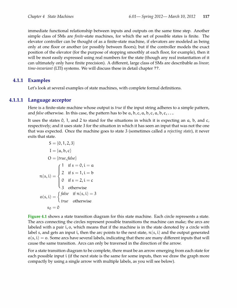
Chapter 4 State Machines 6.01— Spring 2012—March 10, 2012 117
immediate functional relationship between inputs and outputs on the same time step. Anothersimple class of SMs are finite-state machines, for which the set of possible states is finite. Theelevator controller can be thought of as a finite-state machine, if elevators are modeled as beingonly at one floor or another (or possibly between floors); but if the controller models the exactposition of the elevator (for the purpose of stopping smoothly at each floor, for example), then itwill be most easily expressed using real numbers for the state (though any real instantiation of itcan ultimately only have finite precision). A different, large class of SMs are describable as linear,time-invariant (LTI) systems. We will discuss these in detail chapter ??.
4.1.1 ExamplesLet’s look at several examples of state machines, with complete formal definitions.
4.1.1.1 Language acceptorHere is a finite-state machine whose output is true if the input string adheres to a simple pattern,and false otherwise. In this case, the pattern has to be a, b, c, a, b, c, a, b, c, . . ..
It uses the states 0, 1, and 2 to stand for the situations in which it is expecting an a, b, and c,respectively; and it uses state 3 for the situation in which it has seen an input that was not the onethat was expected. Once the machine goes to state 3 (sometimes called a rejecting state), it neverexits that state.
S = 0, 1, 2, 3
I = a, b, c
O = true, false
n(s, i) =
1 if s = 0, i = a
2 if s = 1, i = b
0 if s = 2, i = c
3 otherwise
o(s, i) =
false if n(s, i) = 3
true otherwises0 = 0
Figure 4.1 shows a state transition diagram for this state machine. Each circle represents a state.The arcs connecting the circles represent possible transitions the machine can make; the arcs arelabeled with a pair i, o, which means that if the machine is in the state denoted by a circle withlabel s, and gets an input i, then the arc points to the next state, n(s, i) and the output generatedo(s, i) = o. Some arcs have several labels, indicating that there are many different inputs that willcause the same transition. Arcs can only be traversed in the direction of the arrow.
For a state transition diagram to be complete, there must be an arrow emerging from each state foreach possible input i (if the next state is the same for some inputs, then we draw the graph morecompactly by using a single arrow with multiple labels, as you will see below).

Chapter 4 State Machines 6.01— Spring 2012—March 10, 2012 118
0
3
21
c / True
a / Falseb / False
b / Falsec / False
a / True b / True
a / Falsec / False
a / Falseb / Falsec / False
Figure 4.1 State transition diagram for language acceptor.
We will use tables like the following one to examine the evolution of a state machine:
time 0 1 2 ...
input i0 i1 i2 ...state s0 s1 s2 ...
output o1 o2 o3 ...
For each column in the table, given the current input value and statewe can use the output functiono to determine the output in that column; andwe use then function applied to that input and statevalue to determine the state in the next column. Thus, just knowing the input sequence and s0,and the next-state and output functions of the machine will allow you to fill in the rest of the table.
For example, here is the state of the machine at the initial time point:
time 0 1 2 ...
input i0 ...state s0 ...
output ...
Using our knowledge of the next state function n, we have:
time 0 1 2 ...
input i0 ...state s0 s1 ...
output ...
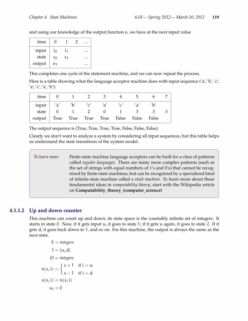
Chapter 4 State Machines 6.01— Spring 2012—March 10, 2012 119
and using our knowledge of the output function o, we have at the next input value
time 0 1 2 ...
input i0 i1 ...state s0 s1 ...
output o1 ...
This completes one cycle of the statement machine, and we can now repeat the process.
Here is a table showing what the language acceptor machine does with input sequence (’a’, ’b’, ’c’,’a’, ’c’, ’a’, ’b’):
time 0 1 2 3 4 5 6 7
input ’a’ ’b’ ’c’ ’a’ ’c’ ’a’ ’b’state 0 1 2 0 1 3 3 3
output True True True True False False False
The output sequence is (True, True, True, True, False, False, False).
Clearly we don’t want to analyze a system by considering all input sequences, but this table helpsus understand the state transitions of the system model.
To learn more: Finite-state machine language acceptors can be built for a class of patternscalled regular languages. There are many more complex patterns (such asthe set of strings with equal numbers of 1’s and 0’s) that cannot be recog-nized by finite-state machines, but can be recognized by a specialized kindof infinite-state machine called a stack machine. To learn more about thesefundamental ideas in computability theory, start with the Wikipedia articleon Computability_theory_(computer_science)
4.1.1.2 Up and down counterThis machine can count up and down; its state space is the countably infinite set of integers. Itstarts in state 0. Now, if it gets input u, it goes to state 1; if it gets u again, it goes to state 2. If itgets d, it goes back down to 1, and so on. For this machine, the output is always the same as thenext state.
S = integers
I = u, d
O = integers
n(s, i) =
s+ 1 if i = u
s− 1 if i = do(s, i) = n(s, i)
s0 = 0

Chapter 4 State Machines 6.01— Spring 2012—March 10, 2012 120
Here is a table showing what the up and down counter does with input sequence u, u, u, d, d, u:
time 0 1 2 3 4 5 6
input u u u d d ustate 0 1 2 3 2 1 2
output 1 2 3 2 1 2
The output sequence is 1, 2, 3, 2, 1, 2.
4.1.1.3 DelayAn even simpler machine just takes the input and passes it through to the output, but with onestep of delay, so the kth element of the input sequence will be the k + 1st element of the outputsequence. Here is the formal machine definition:
S = anything
I = anything
O = anything
n(s, i) = i
o(s, i) = s
s0 = 0
Given an input sequence i0, i1, i2, . . ., this machine will produce an output sequence0, i0, i1, i2, . . .. The initial 0 comes because it has to be able to produce an output before ithas even seen an input, and that output is produced based on the initial state, which is 0. Thisvery simple building block will come in handy for us later on.Here is a table showing what the delay machine does with input sequence 3, 1, 2, 5, 9:
time 0 1 2 3 4 5
input 3 1 2 5 9state 0 3 1 2 5 9
output 0 3 1 2 5
The output sequence is 0, 3, 1, 2, 5.
4.1.1.4 AccumulatorHere is a machine whose output is the sum of all the inputs it has ever seen.
S = numbers
I = numbers
O = numbers
n(s, i) = s+ i
o(s, i) = n(s, i)
s0 = 0
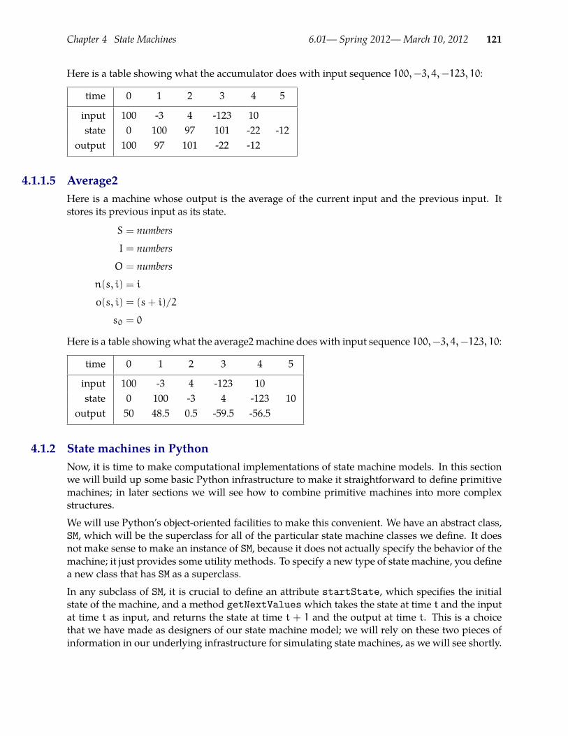
Chapter 4 State Machines 6.01— Spring 2012—March 10, 2012 121
Here is a table showing what the accumulator does with input sequence 100,−3, 4,−123, 10:
time 0 1 2 3 4 5
input 100 -3 4 -123 10state 0 100 97 101 -22 -12
output 100 97 101 -22 -12
4.1.1.5 Average2Here is a machine whose output is the average of the current input and the previous input. Itstores its previous input as its state.
S = numbers
I = numbers
O = numbers
n(s, i) = i
o(s, i) = (s+ i)/2
s0 = 0
Here is a table showing what the average2 machine does with input sequence 100,−3, 4,−123, 10:
time 0 1 2 3 4 5
input 100 -3 4 -123 10state 0 100 -3 4 -123 10
output 50 48.5 0.5 -59.5 -56.5
4.1.2 State machines in PythonNow, it is time to make computational implementations of state machine models. In this sectionwe will build up some basic Python infrastructure to make it straightforward to define primitivemachines; in later sections we will see how to combine primitive machines into more complexstructures.
We will use Python’s object-oriented facilities to make this convenient. We have an abstract class,SM, which will be the superclass for all of the particular state machine classes we define. It doesnot make sense to make an instance of SM, because it does not actually specify the behavior of themachine; it just provides some utility methods. To specify a new type of state machine, you definea new class that has SM as a superclass.
In any subclass of SM, it is crucial to define an attribute startState, which specifies the initialstate of the machine, and a method getNextValueswhich takes the state at time t and the inputat time t as input, and returns the state at time t + 1 and the output at time t. This is a choicethat we have made as designers of our state machine model; we will rely on these two pieces ofinformation in our underlying infrastructure for simulating state machines, as we will see shortly.

Chapter 4 State Machines 6.01— Spring 2012—March 10, 2012 122
Here, for example, is the Python code for an accumulator state machine, which implements thedefinition given in section 4.1.1.4.29
class Accumulator(SM):startState = 0def getNextValues(self, state, inp):
return (state + inp, state + inp)
It is important to note that getNextValues does not change the state of the machine, in other words,it does not mutate a state variable. Its job is to be a pure function: to answer the question of whatthe next state and output would be if the current state were state and the current input wereinp. We will use the getNextValues methods of state machines later in the class to make plansby considering alternative courses of action, so theymust not have any side effects. As we noted, thisis our choice as designers of the state machine infrastructure We could have chosen to implementthings differently, however this choice will prove to be very useful. Thus, in all our state machines,the function getNextValueswill capture the transition from input and state to output and state,without mutating any stored state values.
To run a state machine, we make an instance of the appropriate state-machine class, call its startmethod (a built in method we will see shortly) to set the state to the starting state, and then ask itto take steps; each step consists of generating an output value (which is printed) and updating thestate to the next state, based on the input. The abstract superclass SM defines the start and stepmethods. These methods are in charge of actually initializing and then changing the state of themachine as it is being executed. They do this by calling the getNextValuesmethod for the classto which this instance belongs. The start method takes no arguments (but, even so, we have toput parentheses after it, indicating that we want to call the method, not to do something with themethod itself); the step method takes one argument, which is the input to the machine on the nextstep. So, here is a run of the accumulator, in which we feed it inputs 3, 4, and -2:
>>> a = Accumulator()>>> a.start()>>> a.step(3)3>>> a.step(4)7>>> a.step(-2)5
The class SM specifies how state machines work in general; the class Accumulator specifies howaccumulatormachineswork in general; and the instance a is a particularmachinewith a particularcurrent state. We can make another instance of accumulator:
>>> b = Accumulator()>>> b.start()>>> b.step(10)10>>> b.state
Throughout this code, we use inp, instead of input, which would be clearer. The reason is that the name input is used29
by Python as a function. Although it is legal to re-use it as the name of an argument to a procedure, doing so is a sourceof bugs that are hard to find (if, for instance, youmisspell the name input in the argument list, your references to inputlater in the procedure will be legal, but will return the built-in function.)

Chapter 4 State Machines 6.01— Spring 2012—March 10, 2012 123
10>>> a.state5
Now, we have two accumulators, a, and b, which remember, individually, in what states theyexist. Figure 4.2 shows the class and instance structures that will be in place after creating thesetwo accumulators.
ba
AccumulatorSM
global run
stepstart
transduce
getNextValues
startState 0
5state10state
Figure 4.2 Classes and instances for an Accumulator SM. All of the dots represent procedureobjects.
4.1.2.1 Defining a type of SMLet’s go back to the definition of the Accumulator class, and study it piece by piece.
First, we define the class and say that it is a subclass of SM:
class Accumulator(SM):
Next, we define an attribute of the class, startState, which is the starting state of the machine.In this case, our accumulator starts up with the value 0.
startState = 0
Note that startState is required by the underlying SM class, so we must either define it in oursubclass definition or use a default value from the SM superclass.
The nextmethoddefines both the next-state function and the output function, by taking the currentstate and input as arguments and returning a tuple containing both the next state and the output.
For our accumulator, the next state is just the sum of the previous state and the input; and theoutput is the same thing:
def getNextValues(self, state, inp):return (state + inp, state + inp)
It is crucial that getNextValues be a pure function; that is, that it not change the state of the object(by assigning to any attributes of self). It must simply compute the necessary values and returnthem. We do not promise anything about howmany times this method will be called and in whatcircumstances.

Chapter 4 State Machines 6.01— Spring 2012—March 10, 2012 124
Sometimes, it is convenient to arrange it so that the class really defines a range of machines withslightly different behavior, which depends on some parameters that we set at the timewe create aninstance. So, for example, if we wanted to specify the initial value for an accumulator at the timethe machine is created, we could add an __init__ method30 to our class, which takes an initialvalue as a parameter and uses it to set an attribute called startState of the instance.31
class Accumulator(SM):def __init__(self, initialValue):
self.startState = initialValuedef getNextValues(self, state, inp):
return state + inp, state + inp
Now we can make an accumulator and run it like this:
>>> c = Accumulator(100)>>> c.start()>>> c.step(20)120>>> c.step(2)122
4.1.2.2 The SM ClassThe SM class contains generally useful methods that apply to all state machines. A state machineis an instance of any subclass of SM, that has defined the attribute startState and the methodgetNextValues, as we did for the Accumulator class. Here we examine these methods in moredetail.
Running a machineThe first group of methods allows us to run a state machine. To run a machine is to provide it witha sequence of inputs and then sequentially go forward, computing the next state and generatingthe next output, as if we were filling in a state table.
To run amachine, we have to start by calling the startmethod. All it does is create an attribute ofthe instance, called state, and assign to it the value of the startState attribute. It is crucial thatwe have both of these attributes: if we were to just modify startState, then if we wanted to runthis machine again, we would have permanently forgotten what the starting state should be. Notethat state becomes a repository for the state of this instance; however we should not mutate itdirectly. This variable becomes the internal representation of state for each instance of this class.
class SM:def start(self):
self.state = self.startState
Remember that the __init__method is a special feature of the Python object-oriented system, which is calledwhenever30
an instance of the associated class is created.Note that in the original version of Accumulator, startState was an attribute of the class, since it was the same for31
every instance of the class; now that we want it to be different for different instances, we need startState to be anattribute of the instance rather than the class, which is why we assign it in the __init__ method, which modifies thealready-created instance.
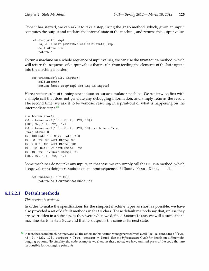
Chapter 4 State Machines 6.01— Spring 2012—March 10, 2012 125
Once it has started, we can ask it to take a step, using the step method, which, given an input,computes the output and updates the internal state of the machine, and returns the output value.
def step(self, inp):(s, o) = self.getNextValues(self.state, inp)self.state = sreturn o
To run a machine on a whole sequence of input values, we can use the transducemethod, whichwill return the sequence of output values that results from feeding the elements of the list inputsinto the machine in order.
def transduce(self, inputs):self.start()return [self.step(inp) for inp in inputs]
Here are the results of running transduce on our accumulatormachine. We run it twice, firstwitha simple call that does not generate any debugging information, and simply returns the result.The second time, we ask it to be verbose, resulting in a print-out of what is happening on theintermediate steps.32
a = Accumulator()>>> a.transduce([100, -3, 4, -123, 10])[100, 97, 101, -22, -12]>>> a.transduce([100, -3, 4, -123, 10], verbose = True)Start state: 0In: 100 Out: 100 Next State: 100In: -3 Out: 97 Next State: 97In: 4 Out: 101 Next State: 101In: -123 Out: -22 Next State: -22In: 10 Out: -12 Next State: -12[100, 97, 101, -22, -12]
Somemachines do not take any inputs; in that case, we can simply call the SM runmethod, whichis equivalent to doing transduce on an input sequence of [None, None, None, ...].
def run(self, n = 10):return self.transduce([None]*n)
4.1.2.2.1 Default methodsThis section is optional.
In order to make the specifications for the simplest machine types as short as possible, we havealso provided a set of default methods in the SM class. These default methods say that, unless theyare overridden in a subclass, as they were when we defined Accumulator, we will assume that amachine starts in state None and that its output is the same as its next state.
In fact, the secondmachine trace, and all the others in this sectionwere generatedwith a call like: a.transduce([100,32
-3, 4, -123, 10], verbose = True, compact = True) See the Infrastructure Guide for details on different de-bugging options. To simplify the code examples we show in these notes, we have omitted parts of the code that areresponsible for debugging printouts.
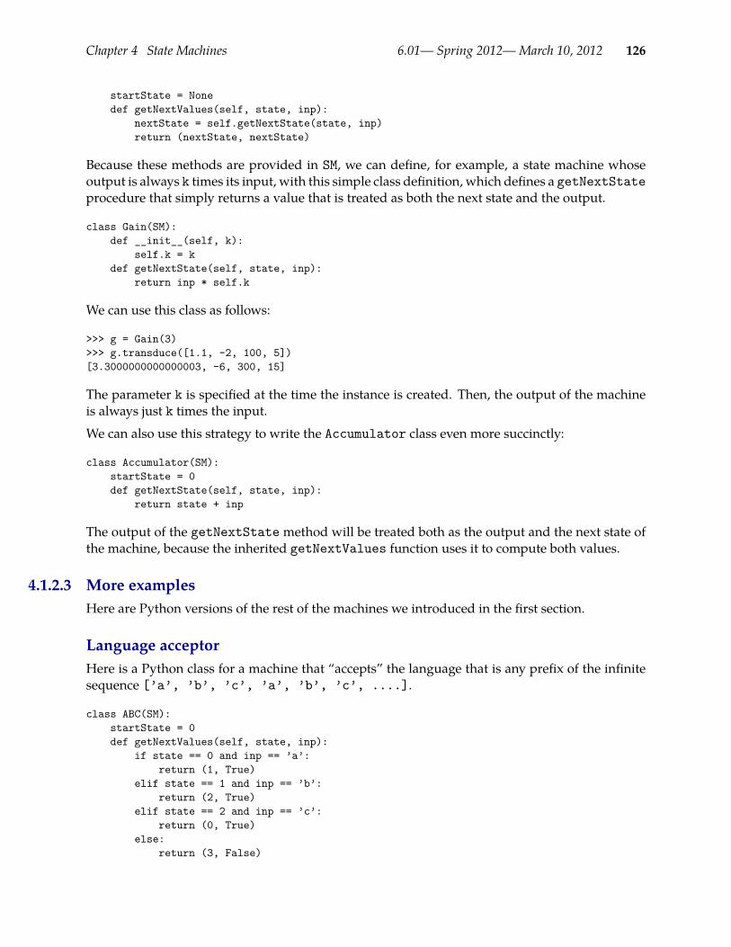
Chapter 4 State Machines 6.01— Spring 2012—March 10, 2012 126
startState = Nonedef getNextValues(self, state, inp):
nextState = self.getNextState(state, inp)return (nextState, nextState)
Because these methods are provided in SM, we can define, for example, a state machine whoseoutput is always k times its input, with this simple class definition, which defines a getNextStateprocedure that simply returns a value that is treated as both the next state and the output.
class Gain(SM):def __init__(self, k):
self.k = kdef getNextState(self, state, inp):
return inp * self.k
We can use this class as follows:
>>> g = Gain(3)>>> g.transduce([1.1, -2, 100, 5])[3.3000000000000003, -6, 300, 15]
The parameter k is specified at the time the instance is created. Then, the output of the machineis always just k times the input.
We can also use this strategy to write the Accumulator class even more succinctly:
class Accumulator(SM):startState = 0def getNextState(self, state, inp):
return state + inp
The output of the getNextStatemethod will be treated both as the output and the next state ofthe machine, because the inherited getNextValues function uses it to compute both values.
4.1.2.3 More examplesHere are Python versions of the rest of the machines we introduced in the first section.
Language acceptorHere is a Python class for a machine that “accepts” the language that is any prefix of the infinitesequence [’a’, ’b’, ’c’, ’a’, ’b’, ’c’, ....].
class ABC(SM):startState = 0def getNextValues(self, state, inp):
if state == 0 and inp == ’a’:return (1, True)
elif state == 1 and inp == ’b’:return (2, True)
elif state == 2 and inp == ’c’:return (0, True)
else:return (3, False)

Chapter 4 State Machines 6.01— Spring 2012—March 10, 2012 127
It behaves as we would expect. As soon as it sees a character that deviates from the desired se-quence, the output is False, and it will remain False for ever after.
>>> abc = ABC()>>> abc.transduce([’a’,’a’,’a’], verbose = True)Start state: 0In: a Out: True Next State: 1In: a Out: False Next State: 3In: a Out: False Next State: 3[True, False, False]
>>> abc.transduce([’a’, ’b’, ’c’, ’a’, ’c’, ’a’, ’b’], verbose = True)Start state: 0In: a Out: True Next State: 1In: b Out: True Next State: 2In: c Out: True Next State: 0In: a Out: True Next State: 1In: c Out: False Next State: 3In: a Out: False Next State: 3In: b Out: False Next State: 3[True, True, True, True, False, False, False]
Count up and downThis is a direct translation of the machine defined in section 4.1.1.2.
class UpDown(SM):startState = 0def getNextState(self, state, inp):
if inp == ’u’:return state + 1
else:return state - 1
We take advantage of the default getNextValues method to make the output the same as thenext state.
>>> ud = UpDown()>>> ud.transduce([’u’,’u’,’u’,’d’,’d’,’u’], verbose = True)Start state: 0In: u Out: 1 Next State: 1In: u Out: 2 Next State: 2In: u Out: 3 Next State: 3In: d Out: 2 Next State: 2In: d Out: 1 Next State: 1In: u Out: 2 Next State: 2[1, 2, 3, 2, 1, 2]
DelayIn order to make a machine that delays its input stream by one time step, we have to specify whatthe first output should be. We do this by passing the parameter, v0, into the __init__ method

Chapter 4 State Machines 6.01— Spring 2012—March 10, 2012 128
of the Delay class. The state of a Delaymachine is just the input from the previous step, and theoutput is the state (which is, therefore, the input from the previous time step).
class Delay(SM):def __init__(self, v0):
self.startState = v0def getNextValues(self, state, inp):
return (inp, state)
>>> d = Delay(7)>>> d.transduce([3, 1, 2, 5, 9], verbose = True)Start state: 7In: 3 Out: 7 Next State: 3In: 1 Out: 3 Next State: 1In: 2 Out: 1 Next State: 2In: 5 Out: 2 Next State: 5In: 9 Out: 5 Next State: 9[7, 3, 1, 2, 5]
>>> d100 = Delay(100)>>> d100.transduce([3, 1, 2, 5, 9], verbose = True)Start state: 100In: 3 Out: 100 Next State: 3In: 1 Out: 3 Next State: 1In: 2 Out: 1 Next State: 2In: 5 Out: 2 Next State: 5In: 9 Out: 5 Next State: 9[100, 3, 1, 2, 5]
Wewill use this machine so frequently that we put its definition in the smmodule (file), alongwiththe class.
RWe can use R as another name for the Delay class of state machines. It will be an importantprimitive in a compositional system of linear time-invariant systems, which we explore in the nextchapter.
Average2Here is a state machine whose output at time t is the average of the input values from times t− 1and t.
class Average2(SM):startState = 0def getNextValues(self, state, inp):
return (inp, (inp + state) / 2.0)
It needs to remember the previous input, so the next state is equal to the input. The output is theaverage of the current input and the state (because the state is the previous input).
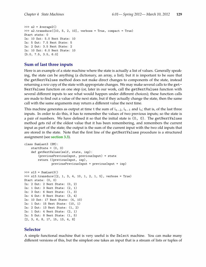
Chapter 4 State Machines 6.01— Spring 2012—March 10, 2012 129
>>> a2 = Average2()>>> a2.transduce([10, 5, 2, 10], verbose = True, compact = True)Start state: 0In: 10 Out: 5.0 Next State: 10In: 5 Out: 7.5 Next State: 5In: 2 Out: 3.5 Next State: 2In: 10 Out: 6.0 Next State: 10[5.0, 7.5, 3.5, 6.0]
Sum of last three inputsHere is an example of a state machine where the state is actually a list of values. Generally speak-ing, the state can be anything (a dictionary, an array, a list); but it is important to be sure thatthe getNextValues method does not make direct changes to components of the state, insteadreturning a new copy of the state with appropriate changes. Wemaymake several calls to the get-NextValues function on one step (or, later in our work, call the getNextValues function withseveral different inputs to see what would happen under different choices); these function callsare made to find out a value of the next state, but if they actually change the state, then the samecall with the same arguments may return a different value the next time.This machine generates as output at time t the sum of it−2, it−1 and it; that is, of the last threeinputs. In order to do this, it has to remember the values of two previous inputs; so the state isa pair of numbers. We have defined it so that the initial state is (0, 0). The getNextValuesmethod gets rid of the oldest value that it has been remembering, and remembers the currentinput as part of the state; the output is the sum of the current input with the two old inputs thatare stored in the state. Note that the first line of the getNextValues procedure is a structuredassignment (see section 3.3).
class SumLast3 (SM):startState = (0, 0)def getNextValues(self, state, inp):
(previousPreviousInput, previousInput) = statereturn ((previousInput, inp),
previousPreviousInput + previousInput + inp)
>>> sl3 = SumLast3()>>> sl3.transduce([2, 1, 3, 4, 10, 1, 2, 1, 5], verbose = True)Start state: (0, 0)In: 2 Out: 2 Next State: (0, 2)In: 1 Out: 3 Next State: (2, 1)In: 3 Out: 6 Next State: (1, 3)In: 4 Out: 8 Next State: (3, 4)In: 10 Out: 17 Next State: (4, 10)In: 1 Out: 15 Next State: (10, 1)In: 2 Out: 13 Next State: (1, 2)In: 1 Out: 4 Next State: (2, 1)In: 5 Out: 8 Next State: (1, 5)[2, 3, 6, 8, 17, 15, 13, 4, 8]
SelectorA simple functional machine that is very useful is the Select machine. You can make manydifferent versions of this, but the simplest one takes an input that is a stream of lists or tuples of

Chapter 4 State Machines 6.01— Spring 2012—March 10, 2012 130
several values (or structures of values) and generates the streammade up only of the kth elementsof the input values. Which particular component this machine is going to select is determined bythe value k, which is passed in at the time the machine instance is initialized.
class Select (SM):def __init__(self, k):
self.k = kdef getNextState(self, state, inp):
return inp[self.k]
4.1.3 Simple parking gate controllerAs one more demonstration, here is a simple example of a finite-state controller for a gate leadingout of a parking lot.
The gate has three sensors:• gatePosition has one of three values ’top’, ’middle’, ’bottom’, signi-
fying the position of the arm of the parking gate.• carAtGate is True if a car is waiting to come through the gate and False
otherwise.• carJustExited is True if a car has just passed through the gate; it is true for
only one step before resetting to False.
Pause to try 4.1. How many possible inputs are there?
A: 12.
The gate has three possible outputs (think of them as controls to the motor for the gate arm):’raise’, ’lower’, and ’nop’. (Nop means “no operation.”)
Roughly, here is what the gate needs to do:• If a car wants to come through, the gate needs to raise the arm until it is at the top position.• Once the gate is at the top position, it has to stay there until the car has driven through the gate.• After the car has driven through the gate needs to lower the arm until it reaches the bottom
position.
So, we have designed a simple finite-state controller with a state transition diagram as shownin figure 4.3. The machine has four possible states: ’waiting’ (for a car to arrive at the gate),’raising’ (the arm), ’raised’ (the arm is at the top position and we’re waiting for the car todrive through the gate), and ’lowering’ (the arm). To keep the figure from being too cluttered,we do not label each arc with every possible input that would cause that transition to be made:instead, we give a condition (think of it as a Boolean expression) that, if true, would cause thetransition to be followed. The conditions on the arcs leading out of each state cover all the possibleinputs, so the machine remains completely well specified.
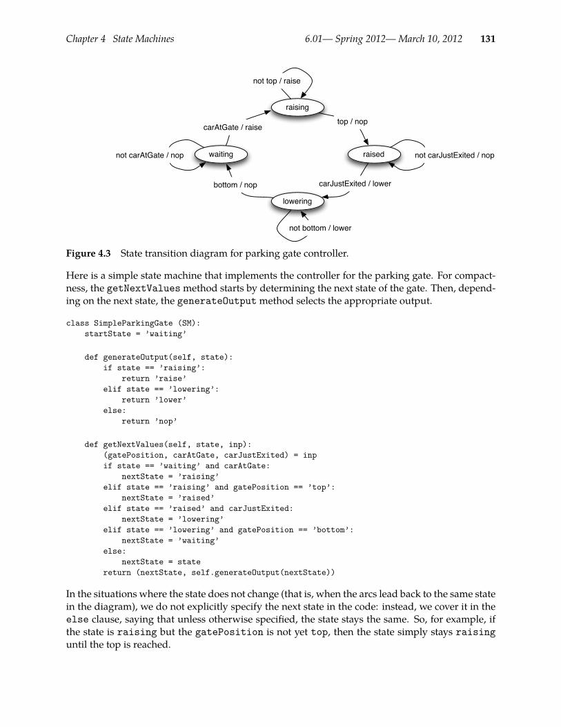
Chapter 4 State Machines 6.01— Spring 2012—March 10, 2012 131
raising
lowering
raisedwaiting
not top / raise
carAtGate / raisetop / nop
carJustExited / lowerbottom / nop
not bottom / lower
not carJustExited / nopnot carAtGate / nop
Figure 4.3 State transition diagram for parking gate controller.
Here is a simple state machine that implements the controller for the parking gate. For compact-ness, the getNextValuesmethod starts by determining the next state of the gate. Then, depend-ing on the next state, the generateOutputmethod selects the appropriate output.
class SimpleParkingGate (SM):startState = ’waiting’
def generateOutput(self, state):if state == ’raising’:
return ’raise’elif state == ’lowering’:
return ’lower’else:
return ’nop’
def getNextValues(self, state, inp):(gatePosition, carAtGate, carJustExited) = inpif state == ’waiting’ and carAtGate:
nextState = ’raising’elif state == ’raising’ and gatePosition == ’top’:
nextState = ’raised’elif state == ’raised’ and carJustExited:
nextState = ’lowering’elif state == ’lowering’ and gatePosition == ’bottom’:
nextState = ’waiting’else:
nextState = statereturn (nextState, self.generateOutput(nextState))
In the situations where the state does not change (that is, when the arcs lead back to the same statein the diagram), we do not explicitly specify the next state in the code: instead, we cover it in theelse clause, saying that unless otherwise specified, the state stays the same. So, for example, ifthe state is raising but the gatePosition is not yet top, then the state simply stays raisinguntil the top is reached.
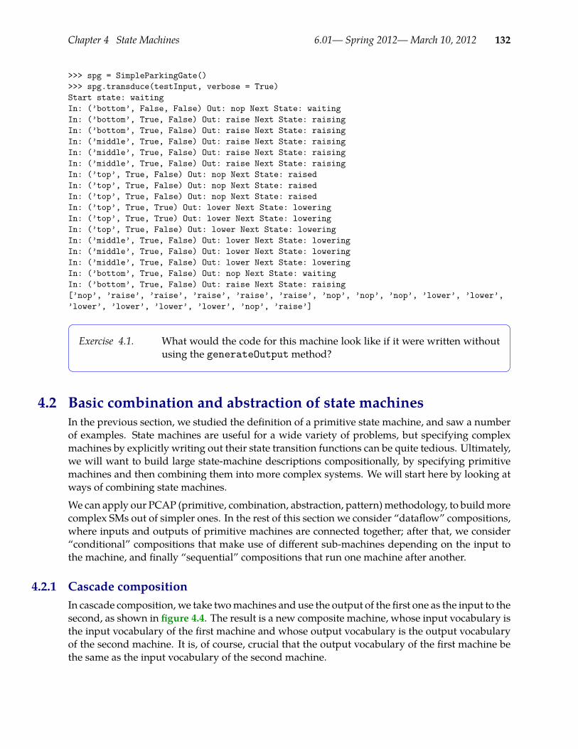
Chapter 4 State Machines 6.01— Spring 2012—March 10, 2012 132
>>> spg = SimpleParkingGate()>>> spg.transduce(testInput, verbose = True)Start state: waitingIn: (’bottom’, False, False) Out: nop Next State: waitingIn: (’bottom’, True, False) Out: raise Next State: raisingIn: (’bottom’, True, False) Out: raise Next State: raisingIn: (’middle’, True, False) Out: raise Next State: raisingIn: (’middle’, True, False) Out: raise Next State: raisingIn: (’middle’, True, False) Out: raise Next State: raisingIn: (’top’, True, False) Out: nop Next State: raisedIn: (’top’, True, False) Out: nop Next State: raisedIn: (’top’, True, False) Out: nop Next State: raisedIn: (’top’, True, True) Out: lower Next State: loweringIn: (’top’, True, True) Out: lower Next State: loweringIn: (’top’, True, False) Out: lower Next State: loweringIn: (’middle’, True, False) Out: lower Next State: loweringIn: (’middle’, True, False) Out: lower Next State: loweringIn: (’middle’, True, False) Out: lower Next State: loweringIn: (’bottom’, True, False) Out: nop Next State: waitingIn: (’bottom’, True, False) Out: raise Next State: raising[’nop’, ’raise’, ’raise’, ’raise’, ’raise’, ’raise’, ’nop’, ’nop’, ’nop’, ’lower’, ’lower’,’lower’, ’lower’, ’lower’, ’lower’, ’nop’, ’raise’]
Exercise 4.1. What would the code for this machine look like if it were written withoutusing the generateOutputmethod?
4.2 Basic combination and abstraction of state machinesIn the previous section, we studied the definition of a primitive state machine, and saw a numberof examples. State machines are useful for a wide variety of problems, but specifying complexmachines by explicitly writing out their state transition functions can be quite tedious. Ultimately,we will want to build large state-machine descriptions compositionally, by specifying primitivemachines and then combining them into more complex systems. We will start here by looking atways of combining state machines.
We can apply our PCAP (primitive, combination, abstraction, pattern)methodology, to buildmorecomplex SMs out of simpler ones. In the rest of this section we consider “dataflow” compositions,where inputs and outputs of primitive machines are connected together; after that, we consider“conditional” compositions that make use of different sub-machines depending on the input tothe machine, and finally “sequential” compositions that run one machine after another.
4.2.1 Cascade compositionIn cascade composition, we take twomachines and use the output of the first one as the input to thesecond, as shown in figure 4.4. The result is a new composite machine, whose input vocabulary isthe input vocabulary of the first machine and whose output vocabulary is the output vocabularyof the second machine. It is, of course, crucial that the output vocabulary of the first machine bethe same as the input vocabulary of the second machine.
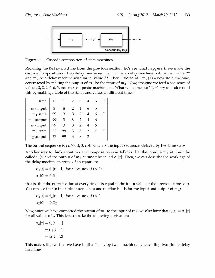
Chapter 4 State Machines 6.01— Spring 2012—March 10, 2012 133
m1 m2o1 = i2i1 o2
Cascade(m1, m2)
Figure 4.4 Cascade composition of state machines
Recalling the Delay machine from the previous section, let’s see what happens if we make thecascade composition of two delay machines. Let m1 be a delay machine with initial value 99and m2 be a delay machine with initial value 22. Then Cascade(m1,m2) is a new state machine,constructed by making the output ofm1 be the input ofm2. Now, imagine we feed a sequence ofvalues, 3, 8, 2, 4, 6, 5, into the composite machine,m. What will come out? Let’s try to understandthis by making a table of the states and values at different times:
time 0 1 2 3 4 5 6
m1 input 3 8 2 4 6 5m1 state 99 3 8 2 4 6 5
m1 output 99 3 8 2 4 6m2 input 99 3 8 2 4 6m2 state 22 99 3 8 2 4 6
m2 output 22 99 3 8 2 4
The output sequence is 22, 99, 3, 8, 2, 4, which is the input sequence, delayed by two time steps.
Another way to think about cascade composition is as follows. Let the input to m1 at time t becalled i1[t] and the output ofm1 at time t be called o1[t]. Then, we can describe the workings ofthe delay machine in terms of an equation:
o1[t] = i1[t− 1] for all values of t > 0;
o1[0] = init1
that is, that the output value at every time t is equal to the input value at the previous time step.You can see that in the table above. The same relation holds for the input and output ofm2:
o2[t] = i2[t− 1] for all values of t > 0.
o2[0] = init2
Now, since we have connected the output ofm1 to the input ofm2, we also have that i2[t] = o1[t]for all values of t. This lets us make the following derivation:
o2[t] = i2[t− 1]
= o1[t− 1]
= i1[t− 2]
This makes it clear that we have built a “delay by two” machine, by cascading two single delaymachines.

Chapter 4 State Machines 6.01— Spring 2012—March 10, 2012 134
As with all of our systems of combination, we will be able to form the cascade composition notonly of two primitive machines, but of any two machines that we can make, through any set ofcompositions of primitive machines.Here is the Python code for an Increment machine. It is a pure function whose output at time tis just the input at time t plus the constant incr. The safeAdd function is the same as addition, ifthe inputs are numbers. We will see, later, why it is important.
class Increment(SM):def __init__(self, incr):
self.incr = incrdef getNextState(self, state, inp):
return safeAdd(inp, self.incr)
Exercise 4.2. Derive what happens when you cascade two delay-by-two machines?
Exercise 4.3. What is the difference between these two machines?
»> foo1 = sm.Cascade(sm.Delay(100), Increment(1))»> foo2 = sm.Cascade(Increment(1), sm.Delay(100))
Demonstrate by drawing a table of their inputs, states, and outputs, overtime.
4.2.2 Parallel compositionIn parallel composition, we take two machines and run them “side by side”. They both take thesame input, and the output of the composite machine is the pair of outputs of the individualmachines. The result is a new composite machine, whose input vocabulary is the same as theinput vocabulary of the component machines (which is the same for both machines) and whoseoutput vocabulary is pairs of elements, the first from the output vocabulary of the first machineand the second from the output vocabulary of the second machine. Figure 4.5 shows two types ofparallel composition; in this section we are talking about the first type.
m1
m2
i
o2
Parallel(m1, m2)
o1 m1
m2
i1
o2
Parallel2(m1, m2)
o1
i2
Figure 4.5 Parallel and Parallel2 compositions of state machines.
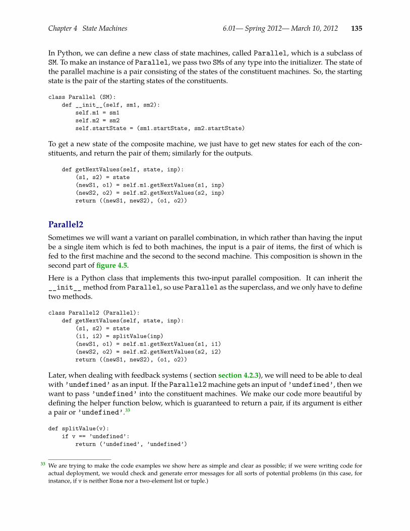
Chapter 4 State Machines 6.01— Spring 2012—March 10, 2012 135
In Python, we can define a new class of state machines, called Parallel, which is a subclass ofSM. To make an instance of Parallel, we pass two SMs of any type into the initializer. The state ofthe parallel machine is a pair consisting of the states of the constituent machines. So, the startingstate is the pair of the starting states of the constituents.
class Parallel (SM):def __init__(self, sm1, sm2):
self.m1 = sm1self.m2 = sm2self.startState = (sm1.startState, sm2.startState)
To get a new state of the composite machine, we just have to get new states for each of the con-stituents, and return the pair of them; similarly for the outputs.
def getNextValues(self, state, inp):(s1, s2) = state(newS1, o1) = self.m1.getNextValues(s1, inp)(newS2, o2) = self.m2.getNextValues(s2, inp)return ((newS1, newS2), (o1, o2))
Parallel2Sometimes we will want a variant on parallel combination, in which rather than having the inputbe a single item which is fed to both machines, the input is a pair of items, the first of which isfed to the first machine and the second to the second machine. This composition is shown in thesecond part of figure 4.5.
Here is a Python class that implements this two-input parallel composition. It can inherit the__init__method from Parallel, so use Parallel as the superclass, andwe only have to definetwo methods.
class Parallel2 (Parallel):def getNextValues(self, state, inp):
(s1, s2) = state(i1, i2) = splitValue(inp)(newS1, o1) = self.m1.getNextValues(s1, i1)(newS2, o2) = self.m2.getNextValues(s2, i2)return ((newS1, newS2), (o1, o2))
Later, when dealing with feedback systems ( section section 4.2.3), we will need to be able to dealwith ’undefined’ as an input. If the Parallel2machine gets an input of ’undefined’, thenwewant to pass ’undefined’ into the constituent machines. We make our code more beautiful bydefining the helper function below, which is guaranteed to return a pair, if its argument is eithera pair or ’undefined’.33
def splitValue(v):if v == ’undefined’:
return (’undefined’, ’undefined’)
We are trying to make the code examples we show here as simple and clear as possible; if we were writing code for33
actual deployment, we would check and generate error messages for all sorts of potential problems (in this case, forinstance, if v is neither None nor a two-element list or tuple.)

Chapter 4 State Machines 6.01— Spring 2012—March 10, 2012 136
else:return v
ParallelAddThe ParallelAdd state machine combination is just like Parallel, except that it has a singleoutput whose value is the sum of the outputs of the constituent machines. It is straightforward todefine:
class ParallelAdd (Parallel):def getNextValues(self, state, inp):
(s1, s2) = state(newS1, o1) = self.m1.getNextValues(s1, inp)(newS2, o2) = self.m2.getNextValues(s2, inp)return ((newS1, newS2), o1 + o2)
4.2.3 Feedback composition
m
Feedback(m)
o m
Feedback2(m)
oi
Figure 4.6 Two forms of feedback composition.
Another important means of combination that we will use frequently is the feedback combinator,in which the output of a machine is fed back to be the input of the same machine at the next step,as shown in figure 4.6. The first value that is fed back is the output associated with the initial stateof the machine on which we are operating. It is crucial that the input and output vocabularies ofthe machine are the same (because the output at step t will be the input at step t + 1). Becausewe have fed the output back to the input, this machine does not consume any inputs; but we willtreat the feedback value as an output of this machine.
Here is an example of using feedback to make a machine that counts. We can start with a simplemachine, an incrementer, that takes a number as input and returns that same number plus 1 as theoutput. By itself, it has no memory. Here is its formal description:
S = numbers
I = numbers
O = numbers
n(s, i) = i+ 1
o(s, i) = n(s, i)
s0 = 0

Chapter 4 State Machines 6.01— Spring 2012—March 10, 2012 137
What would happen if we performed the feedback operation on this machine? We can try tounderstand this in terms of the input/output equations. From the definition of the incrementmachine, we have
o[t] = i[t] + 1 .
And if we connect the input to the output, then we will have
i[t] = o[t] .
And so, we have a problem; these equations cannot be satisfied.
A crucial requirement for applying feedback to a machine is: that machine must not have a directdependence of its output on its input.
Incr Delay(0)
Counter
Figure 4.7 Counter made with feedback and serial combination of an incrementer and a delay.
We have already explored a Delay machine, which delays its output by one step. We can delaythe result of our incrementer, by cascading it with a Delaymachine, as shown in figure 4.7. Now,we have the following equations describing the system:
oi[t] = ii[t] + 1
od[t] = id[t− 1]
ii[t] = od[t]
id[t] = oi[t]
The first two equations describe the operations of the increment and delay boxes; the second twodescribe the wiring between the modules. Now we can see that, in general,
oi[t] = ii[t] + 1
oi[t] = od[t] + 1
oi[t] = id[t− 1] + 1
oi[t] = oi[t− 1] + 1
that is, that the output of the incrementer is going to be one greater on each time step.
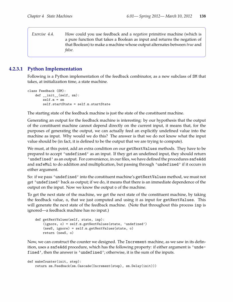
Chapter 4 State Machines 6.01— Spring 2012—March 10, 2012 138
Exercise 4.4. How could you use feedback and a negation primitive machine (which isa pure function that takes a Boolean as input and returns the negation ofthat Boolean) tomake amachine whose output alternates between true andfalse.
4.2.3.1 Python ImplementationFollowing is a Python implementation of the feedback combinator, as a new subclass of SM thattakes, at initialization time, a state machine.
class Feedback (SM):def __init__(self, sm):
self.m = smself.startState = self.m.startState
The starting state of the feedback machine is just the state of the constituent machine.
Generating an output for the feedback machine is interesting: by our hypothesis that the outputof the constituent machine cannot depend directly on the current input, it means that, for thepurposes of generating the output, we can actually feed an explicitly undefined value into themachine as input. Why would we do this? The answer is that we do not know what the inputvalue should be (in fact, it is defined to be the output that we are trying to compute).
We must, at this point, add an extra condition on our getNextValuesmethods. They have to beprepared to accept ’undefined’ as an input. If they get an undefined input, they should return’undefined’ as an output. For convenience, in our files, we have defined the procedures safeAddand safeMul to do addition and multiplication, but passing through ’undefined’ if it occurs ineither argument.
So: if we pass ’undefined’ into the constituent machine’s getNextValuesmethod, wemust notget ’undefined’ back as output; if we do, it means that there is an immediate dependence of theoutput on the input. Now we know the output o of the machine.
To get the next state of the machine, we get the next state of the constituent machine, by takingthe feedback value, o, that we just computed and using it as input for getNextValues. Thiswill generate the next state of the feedback machine. (Note that throughout this process inp isignored—a feedback machine has no input.)
def getNextValues(self, state, inp):(ignore, o) = self.m.getNextValues(state, ’undefined’)(newS, ignore) = self.m.getNextValues(state, o)return (newS, o)
Now, we can construct the counter we designed. The Incrementmachine, as we saw in its defin-ition, uses a safeAdd procedure, which has the following property: if either argument is ’unde-fined’, then the answer is ’undefined’; otherwise, it is the sum of the inputs.
def makeCounter(init, step):return sm.Feedback(sm.Cascade(Increment(step), sm.Delay(init)))
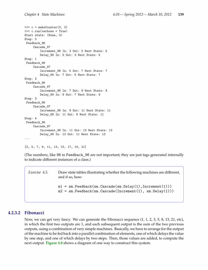
Chapter 4 State Machines 6.01— Spring 2012—March 10, 2012 139
>>> c = makeCounter(3, 2)>>> c.run(verbose = True)Start state: (None, 3)Step: 0Feedback_96
Cascade_97Increment_98 In: 3 Out: 5 Next State: 5Delay_99 In: 5 Out: 3 Next State: 5
Step: 1Feedback_96
Cascade_97Increment_98 In: 5 Out: 7 Next State: 7Delay_99 In: 7 Out: 5 Next State: 7
Step: 2Feedback_96
Cascade_97Increment_98 In: 7 Out: 9 Next State: 9Delay_99 In: 9 Out: 7 Next State: 9
Step: 3Feedback_96
Cascade_97Increment_98 In: 9 Out: 11 Next State: 11Delay_99 In: 11 Out: 9 Next State: 11
Step: 4Feedback_96
Cascade_97Increment_98 In: 11 Out: 13 Next State: 13Delay_99 In: 13 Out: 11 Next State: 13
...
[3, 5, 7, 9, 11, 13, 15, 17, 19, 21]
(The numbers, like 96 in Feedback_96 are not important; they are just tags generated internallyto indicate different instances of a class.)
Exercise 4.5. Draw state tables illustratingwhether the followingmachines are different,and if so, how:
m1 = sm.Feedback(sm.Cascade(sm.Delay(1),Increment(1)))m2 = sm.Feedback(sm.Cascade(Increment(1), sm.Delay(1)))
4.2.3.2 FibonacciNow, we can get very fancy. We can generate the Fibonacci sequence (1, 1, 2, 3, 5, 8, 13, 21, etc),in which the first two outputs are 1, and each subsequent output is the sum of the two previousoutputs, using a combination of very simplemachines. Basically, we have to arrange for the outputof themachine to be fed back into a parallel combination of elements, one ofwhich delays the valueby one step, and one of which delays by two steps. Then, those values are added, to compute thenext output. Figure 4.8 shows a diagram of one way to construct this system.
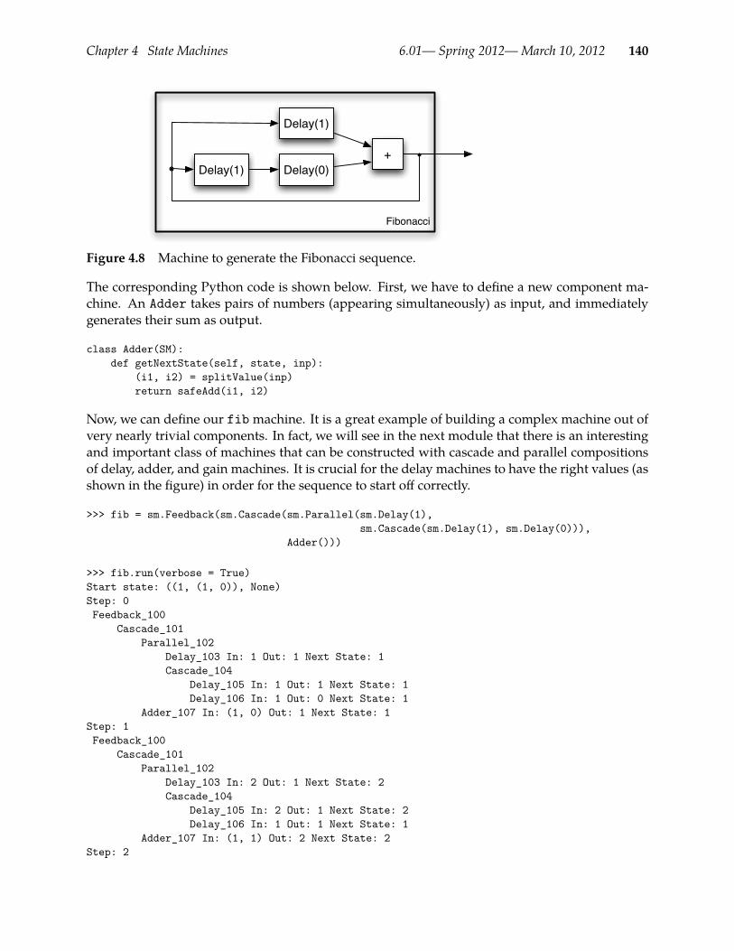
Chapter 4 State Machines 6.01— Spring 2012—March 10, 2012 140
Delay(1) Delay(0)
Fibonacci
Delay(1)
+
Figure 4.8 Machine to generate the Fibonacci sequence.
The corresponding Python code is shown below. First, we have to define a new component ma-chine. An Adder takes pairs of numbers (appearing simultaneously) as input, and immediatelygenerates their sum as output.
class Adder(SM):def getNextState(self, state, inp):
(i1, i2) = splitValue(inp)return safeAdd(i1, i2)
Now, we can define our fibmachine. It is a great example of building a complex machine out ofvery nearly trivial components. In fact, we will see in the next module that there is an interestingand important class of machines that can be constructed with cascade and parallel compositionsof delay, adder, and gain machines. It is crucial for the delay machines to have the right values (asshown in the figure) in order for the sequence to start off correctly.
>>> fib = sm.Feedback(sm.Cascade(sm.Parallel(sm.Delay(1),sm.Cascade(sm.Delay(1), sm.Delay(0))),
Adder()))
>>> fib.run(verbose = True)Start state: ((1, (1, 0)), None)Step: 0Feedback_100
Cascade_101Parallel_102
Delay_103 In: 1 Out: 1 Next State: 1Cascade_104
Delay_105 In: 1 Out: 1 Next State: 1Delay_106 In: 1 Out: 0 Next State: 1
Adder_107 In: (1, 0) Out: 1 Next State: 1Step: 1Feedback_100
Cascade_101Parallel_102
Delay_103 In: 2 Out: 1 Next State: 2Cascade_104
Delay_105 In: 2 Out: 1 Next State: 2Delay_106 In: 1 Out: 1 Next State: 1
Adder_107 In: (1, 1) Out: 2 Next State: 2Step: 2
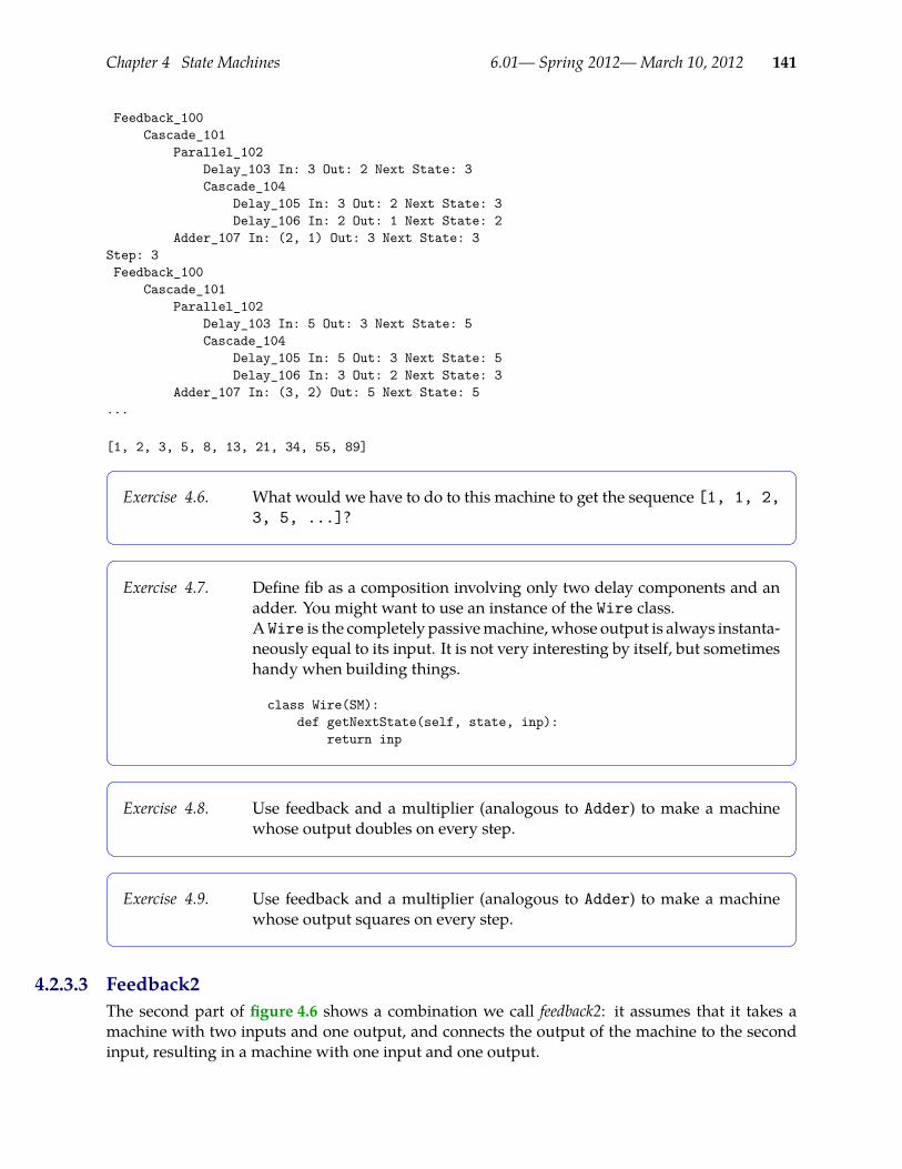
Chapter 4 State Machines 6.01— Spring 2012—March 10, 2012 141
Feedback_100Cascade_101
Parallel_102Delay_103 In: 3 Out: 2 Next State: 3Cascade_104
Delay_105 In: 3 Out: 2 Next State: 3Delay_106 In: 2 Out: 1 Next State: 2
Adder_107 In: (2, 1) Out: 3 Next State: 3Step: 3Feedback_100
Cascade_101Parallel_102
Delay_103 In: 5 Out: 3 Next State: 5Cascade_104
Delay_105 In: 5 Out: 3 Next State: 5Delay_106 In: 3 Out: 2 Next State: 3
Adder_107 In: (3, 2) Out: 5 Next State: 5...
[1, 2, 3, 5, 8, 13, 21, 34, 55, 89]
Exercise 4.6. What would we have to do to this machine to get the sequence [1, 1, 2,3, 5, ...]?
Exercise 4.7. Define fib as a composition involving only two delay components and anadder. You might want to use an instance of the Wire class.A Wire is the completely passivemachine, whose output is always instanta-neously equal to its input. It is not very interesting by itself, but sometimeshandy when building things.
class Wire(SM):def getNextState(self, state, inp):
return inp
Exercise 4.8. Use feedback and a multiplier (analogous to Adder) to make a machinewhose output doubles on every step.
Exercise 4.9. Use feedback and a multiplier (analogous to Adder) to make a machinewhose output squares on every step.
4.2.3.3 Feedback2The second part of figure 4.6 shows a combination we call feedback2: it assumes that it takes amachine with two inputs and one output, and connects the output of the machine to the secondinput, resulting in a machine with one input and one output.
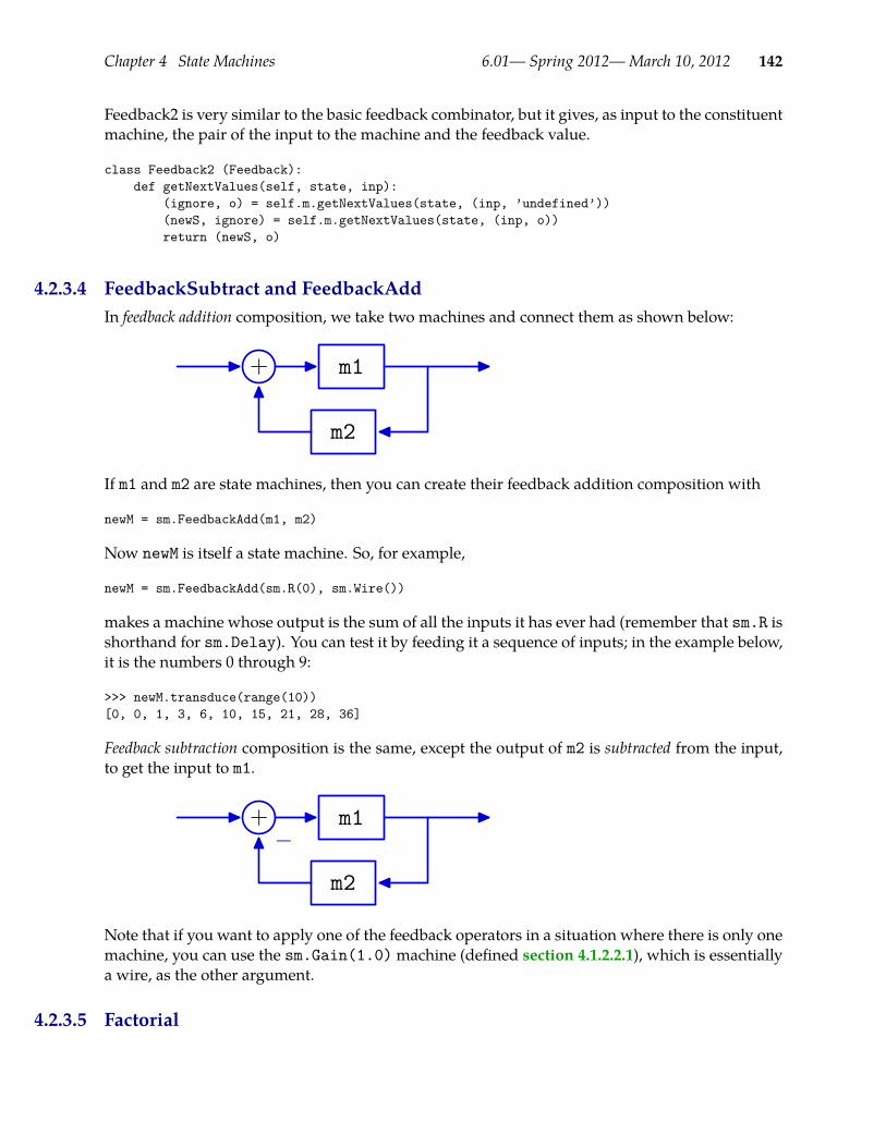
Chapter 4 State Machines 6.01— Spring 2012—March 10, 2012 142
Feedback2 is very similar to the basic feedback combinator, but it gives, as input to the constituentmachine, the pair of the input to the machine and the feedback value.
class Feedback2 (Feedback):def getNextValues(self, state, inp):
(ignore, o) = self.m.getNextValues(state, (inp, ’undefined’))(newS, ignore) = self.m.getNextValues(state, (inp, o))return (newS, o)
4.2.3.4 FeedbackSubtract and FeedbackAddIn feedback addition composition, we take two machines and connect them as shown below:
m1
m2
+
If m1 and m2 are state machines, then you can create their feedback addition composition with
newM = sm.FeedbackAdd(m1, m2)
Now newM is itself a state machine. So, for example,
newM = sm.FeedbackAdd(sm.R(0), sm.Wire())
makes a machine whose output is the sum of all the inputs it has ever had (remember that sm.R isshorthand for sm.Delay). You can test it by feeding it a sequence of inputs; in the example below,it is the numbers 0 through 9:
>>> newM.transduce(range(10))[0, 0, 1, 3, 6, 10, 15, 21, 28, 36]
Feedback subtraction composition is the same, except the output of m2 is subtracted from the input,to get the input to m1.
m1
m2
+−
Note that if you want to apply one of the feedback operators in a situation where there is only onemachine, you can use the sm.Gain(1.0)machine (defined section 4.1.2.2.1), which is essentiallya wire, as the other argument.
4.2.3.5 Factorial

Chapter 4 State Machines 6.01— Spring 2012—March 10, 2012 143
We will do one more tricky example, and illustrate the use of Feedback2. What if wewanted to generate the sequence of numbers 1!, 2!, 3!, 4!, . . . (where k! = 1 · 2 · 3 . . . · k)?We can do so by multiplying the previous value of the sequence by a number equal to the“index” of the sequence. Figure 4.9 shows the structure of a machine for solving this problem. Ituses a counter (which is, as we saw before, made with feedback around a delay and increment)as the input to a machine that takes a single input, and multiplies it by the output value of themachine, fed back through a delay.
Incr Delay(1)
Factorial
* Delay(1)
Counter
Figure 4.9 Machine to generate the Factorial sequence.
Here is how to do it in Python; we take advantage of having defined counter machines to abstractaway from them and use that definition here without thinking about its internal structure. Theinitial values in the delays get the series started off in the right place. What would happen if westarted at 0?
fact = sm.Cascade(makeCounter(1, 1),sm.Feedback2(sm.Cascade(Multiplier(), sm.Delay(1))))
>>> fact.run(verbose = True)Start state: ((None, 1), (None, 1))Step: 0Cascade_1
Feedback_2Cascade_3
Increment_4 In: 1 Out: 2 Next State: 2Delay_5 In: 2 Out: 1 Next State: 2
Feedback2_6Cascade_7
Multiplier_8 In: (1, 1) Out: 1 Next State: 1Delay_9 In: 1 Out: 1 Next State: 1
Step: 1Cascade_1
Feedback_2Cascade_3
Increment_4 In: 2 Out: 3 Next State: 3Delay_5 In: 3 Out: 2 Next State: 3
Feedback2_6Cascade_7
Multiplier_8 In: (2, 1) Out: 2 Next State: 2Delay_9 In: 2 Out: 1 Next State: 2
Step: 2Cascade_1
Feedback_2
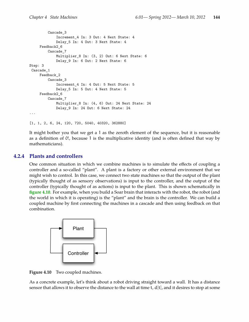
Chapter 4 State Machines 6.01— Spring 2012—March 10, 2012 144
Cascade_3Increment_4 In: 3 Out: 4 Next State: 4Delay_5 In: 4 Out: 3 Next State: 4
Feedback2_6Cascade_7
Multiplier_8 In: (3, 2) Out: 6 Next State: 6Delay_9 In: 6 Out: 2 Next State: 6
Step: 3Cascade_1
Feedback_2Cascade_3
Increment_4 In: 4 Out: 5 Next State: 5Delay_5 In: 5 Out: 4 Next State: 5
Feedback2_6Cascade_7
Multiplier_8 In: (4, 6) Out: 24 Next State: 24Delay_9 In: 24 Out: 6 Next State: 24
...
[1, 1, 2, 6, 24, 120, 720, 5040, 40320, 362880]
It might bother you that we get a 1 as the zeroth element of the sequence, but it is reasonableas a definition of 0!, because 1 is the multiplicative identity (and is often defined that way bymathematicians).
4.2.4 Plants and controllersOne common situation in which we combine machines is to simulate the effects of coupling acontroller and a so-called “plant”. A plant is a factory or other external environment that wemight wish to control. In this case, we connect two state machines so that the output of the plant(typically thought of as sensory observations) is input to the controller, and the output of thecontroller (typically thought of as actions) is input to the plant. This is shown schematically infigure 4.10. For example, when you build a Soar brain that interacts with the robot, the robot (andthe world in which it is operating) is the “plant” and the brain is the controller. We can build acoupled machine by first connecting the machines in a cascade and then using feedback on thatcombination.
Plant
Controller
Figure 4.10 Two coupled machines.
As a concrete example, let’s think about a robot driving straight toward a wall. It has a distancesensor that allows it to observe the distance to the wall at time t, d[t], and it desires to stop at some
Chapter 4 State Machines 6.01— Spring 2012—March 10, 2012 145
distance ddesired. The robot can execute velocity commands, andwe program it to use the followingrule to set its velocity at time t, based on its most recent sensor reading:
v[t] = K(ddesired − d[t− 1]) .
This controller can also be described as a state machine, whose input sequence is the observedvalues of d and whose output sequence is the values of v.
S = numbers
I = numbers
O = numbers
n(s, i) = K(ddesired − i)
o(s) = s
s0 = dinit
Now, we can think about the “plant”; that is, the relationship between the robot and the world.The distance of the robot to the wall changes at each time step depending on the robot’s forwardvelocity and the length of the time steps. Let δT be the length of time between velocity commandsissued by the robot. Then we can describe the world with the equation:
d[t] = d[t− 1] − δTv[t− 1] .
which assumes that a positive velocity moves the robot toward the wall (and therefore decreasesthe distance). This system can be described as a state machine, whose input sequence is the valuesof the robot’s velocity, v, and whose output sequence is the values of its distance to the wall, d.Finally, we can couple these two systems, as for a simulator, to get a single state machine with noinputs. We can observe the sequence of internal values of d and v to understand how the systemis behaving.In Python, we start by defining the controller machine; the values k and dDesired are constantsof the whole system.
k = -1.5dDesired = 1.0class WallController(SM):
def getNextState(self, state, inp):return safeMul(k, safeAdd(dDesired, safeMul(-1, inp)))
The output being generated is actually k * (dDesired - inp), but because thismethod is goingto be used in a feedback machine, it might have to deal with ’undefined’ as an input. It has nodelay built into it.Think about why we want k to be negative. What happens when the robot is closer to the wallthan desired? What happens when it is farther from the wall than desired?Now, we can define a class that describes the behavior of the “plant”:
deltaT = 0.1class WallWorld(SM):
startState = 5def getNextValues(self, state, inp):
return (state - deltaT * inp, state)

Chapter 4 State Machines 6.01— Spring 2012—March 10, 2012 146
Setting startState = 5means that the robot starts 5 meters from the wall. Note that the outputof this machine does not depend instantaneously on the input; so there is a delay in it.
Now, we can defined a general combinator for coupling twomachines, as in a plant and controller:
def coupledMachine(m1, m2):return sm.Feedback(sm.Cascade(m1, m2))
We can use it to connect our controller to the world, and run it:
>>> wallSim = coupledMachine(WallController(), WallWorld())>>> wallSim.run(30)[5, 4.4000000000000004, 3.8900000000000001, 3.4565000000000001,3.088025, 2.77482125, 2.5085980624999999, 2.2823083531249999,2.0899621001562498, 1.9264677851328122, 1.7874976173628905,1.6693729747584569, 1.5689670285446884, 1.483621974262985,1.4110786781235374, 1.3494168764050067, 1.2970043449442556,1.2524536932026173, 1.2145856392222247, 1.1823977933388909,1.1550381243380574, 1.1317824056873489, 1.1120150448342465,1.0952127881091096, 1.0809308698927431, 1.0687912394088317,1.058472553497507, 1.049701670472881, 1.0422464199019488,1.0359094569166565]
Because WallWorld is the second machine in the cascade, its output is the output of the wholemachine; so, we can see that the distance from the robot to the wall is converging monotonicallyto dDesired (which is 1).
Exercise 4.10. What kind of behavior do you get with different values of k?
4.2.5 ConditionalsWemightwant to use differentmachines depending on something that is happening in the outsideworld. Here we describe three different conditional combinators, that make choices, at the run-time of the machine, about what to do.
4.2.6 SwitchWe will start by considering a conditional combinator that runs two machines in parallel, butdecides on every inputwhether to send the input into one machine or the other. So, only one of theparallel machines has its state updated on each step. We will call this switch, to emphasize the factthat the decision about which machine to execute is being re-made on every step.
Implementing this requires us to maintain the states of both machines, just as we did for parallelcombination. The getNextValuesmethod tests the condition and then gets a new state and out-put from the appropriate constituent machine; it also has to be sure to pass through the old statefor the constituent machine that was not updated this time.
class Switch (SM):def __init__(self, condition, sm1, sm2):
self.m1 = sm1self.m2 = sm2
Chapter 4 State Machines 6.01— Spring 2012—March 10, 2012 147
self.condition = conditionself.startState = (self.m1.startState, self.m2.startState)
def getNextValues(self, state, inp):(s1, s2) = stateif self.condition(inp):
(ns1, o) = self.m1.getNextValues(s1, inp)return ((ns1, s2), o)
else:(ns2, o) = self.m2.getNextValues(s2, inp)return ((s1, ns2), o)
MultiplexThe switch combinator takes care to only update one of the component machines; in some othercases, we want to update both machines on every step and simply use the condition to select theoutput of one machine or the other to be the current output of the combined machine.This is a very small variation on Switch, so we will just implement it as a subclass.
class Mux (Switch):def getNextValues(self, state, inp):
(s1, s2) = state(ns1, o1) = self.m1.getNextValues(s1, inp)(ns2, o2) = self.m2.getNextValues(s2, inp)if self.condition(inp):
return ((ns1, ns2), o1)else:
return ((ns1, ns2), o2)
Exercise 4.11. What is the result of running these two machines
m1 = Switch(lambda inp: inp > 100,Accumulator(),Accumulator())
m2 = Mux(lambda inp: inp > 100,Accumulator(),Accumulator())
on the input
[2, 3, 4, 200, 300, 400, 1, 2, 3]
Explain why they are the same or are different.
IfFeel free to skip this example; it is only useful in fairly complicated contexts.The If combinator. It takes a condition, which is a function from the input to true or false, andtwo machines. It evaluates the condition on the first input it receives. If the value is truethen it executes the first machine forever more; if it is false, then it executes the second machine.
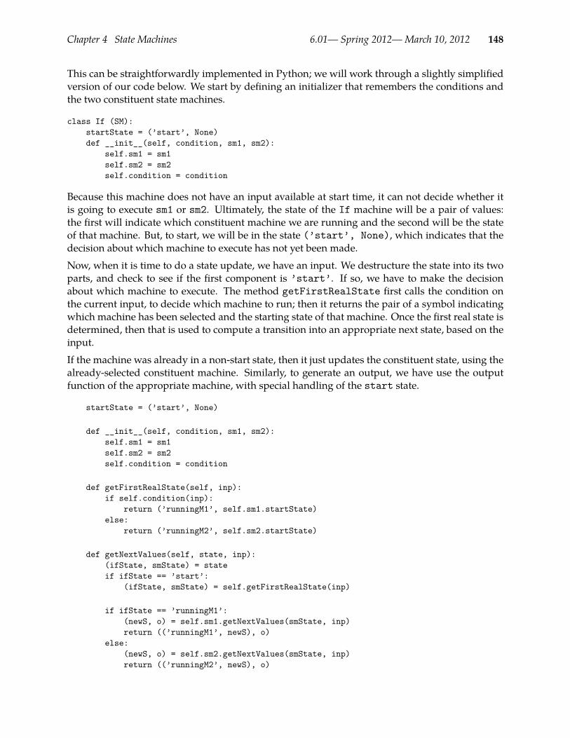
Chapter 4 State Machines 6.01— Spring 2012—March 10, 2012 148
This can be straightforwardly implemented in Python; we will work through a slightly simplifiedversion of our code below. We start by defining an initializer that remembers the conditions andthe two constituent state machines.
class If (SM):startState = (’start’, None)def __init__(self, condition, sm1, sm2):
self.sm1 = sm1self.sm2 = sm2self.condition = condition
Because this machine does not have an input available at start time, it can not decide whether itis going to execute sm1 or sm2. Ultimately, the state of the If machine will be a pair of values:the first will indicate which constituent machine we are running and the second will be the stateof that machine. But, to start, we will be in the state (’start’, None), which indicates that thedecision about which machine to execute has not yet been made.
Now, when it is time to do a state update, we have an input. We destructure the state into its twoparts, and check to see if the first component is ’start’. If so, we have to make the decisionabout which machine to execute. The method getFirstRealState first calls the condition onthe current input, to decide which machine to run; then it returns the pair of a symbol indicatingwhich machine has been selected and the starting state of that machine. Once the first real state isdetermined, then that is used to compute a transition into an appropriate next state, based on theinput.
If the machine was already in a non-start state, then it just updates the constituent state, using thealready-selected constituent machine. Similarly, to generate an output, we have use the outputfunction of the appropriate machine, with special handling of the start state.
startState = (’start’, None)
def __init__(self, condition, sm1, sm2):self.sm1 = sm1self.sm2 = sm2self.condition = condition
def getFirstRealState(self, inp):if self.condition(inp):
return (’runningM1’, self.sm1.startState)else:
return (’runningM2’, self.sm2.startState)
def getNextValues(self, state, inp):(ifState, smState) = stateif ifState == ’start’:
(ifState, smState) = self.getFirstRealState(inp)
if ifState == ’runningM1’:(newS, o) = self.sm1.getNextValues(smState, inp)return ((’runningM1’, newS), o)
else:(newS, o) = self.sm2.getNextValues(smState, inp)return ((’runningM2’, newS), o)

Chapter 4 State Machines 6.01— Spring 2012—March 10, 2012 149
4.3 Terminating state machines and sequential compositionsSo far, all the machines we have discussed run forever; or, at least, until we quit giving theminputs. But in some cases, it is particularly useful to think of a process as consisting of a sequenceof processes, one executing until termination, and then another one starting. For example, youmight want to robot to clean first room A, and then clean room B; or, for it to search in an areauntil it finds a person and then sound an alarm.
Temporal combinations of machines form a new, different PCAP system for state machines. Ourprimitives will be state machines, as described above, but with one additional property: they willhave a termination or done function, d(s), which takes a state and returns true if the machine hasfinished execution and false otherwise.
Rather than defining a whole new class of state machines (though we could do that), we willjust augment the SM class with a default method, which says that, by default, machines do notterminate.
def done(self, state):return False
Then, in the definition of any subclass of SM, you are free to implement your own done methodthat will override this base one. The donemethod is used by state machine combinators that, forexample, run one machine until it is done, and then switch to running another one.
Here is an example terminating state machine (TSM) that consumes a stream of numbers; its outputis None on the first four steps and then on the fifth step, it generates the sum of the numbers it hasseen as inputs, and then terminates. It looks just like the state machines we have seen before, withthe addition of a donemethod. Its state consists of two numbers: the first is the number of timesthe machine has been updated and the second is the total input it has accumulated so far.
class ConsumeFiveValues(SM):startState = (0, 0) # count, total
def getNextValues(self, state, inp):(count, total) = stateif count == 4:
return ((count + 1, total + inp), total + inp)else:
return ((count + 1, total + inp), None)
def done(self, state):(count, total) = statereturn count == 5
Here is the result of running a simple example. We have modified the transduce method of SMto stop when the machine is done.
>>> c5 = ConsumeFiveValues()>>> c5.transduce([1, 2, 3, 4, 5, 6, 7, 8, 9, 10], verbose = True)Start state: (0, 0)In: 1 Out: None Next State: (1, 1)In: 2 Out: None Next State: (2, 3)In: 3 Out: None Next State: (3, 6)
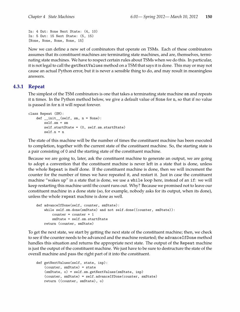
Chapter 4 State Machines 6.01— Spring 2012—March 10, 2012 150
In: 4 Out: None Next State: (4, 10)In: 5 Out: 15 Next State: (5, 15)[None, None, None, None, 15]
Now we can define a new set of combinators that operate on TSMs. Each of these combinatorsassumes that its constituent machines are terminating state machines, and are, themselves, termi-nating state machines. We have to respect certain rules about TSMswhenwe do this. In particular,it is not legal to call the getNextValuesmethod on a TSM that says it is done. Thismay ormay notcause an actual Python error, but it is never a sensible thing to do, and may result in meaninglessanswers.
4.3.1 RepeatThe simplest of the TSM combinators is one that takes a terminating state machine sm and repeatsit n times. In the Python method below, we give a default value of None for n, so that if no valueis passed in for n it will repeat forever.
class Repeat (SM):def __init__(self, sm, n = None):
self.sm = smself.startState = (0, self.sm.startState)self.n = n
The state of this machine will be the number of times the constituent machine has been executedto completion, together with the current state of the constituent machine. So, the starting state isa pair consisting of 0 and the starting state of the constituent machine.Because we are going to, later, ask the constituent machine to generate an output, we are goingto adopt a convention that the constituent machine is never left in a state that is done, unlessthe whole Repeat is itself done. If the constituent machine is done, then we will increment thecounter for the number of times we have repeated it, and restart it. Just in case the constituentmachine “wakes up” in a state that is done, we use a while loop here, instead of an if: we willkeep restarting this machine until the count runs out. Why? Because we promised not to leave ourconstituent machine in a done state (so, for example, nobody asks for its output, when its done),unless the whole repeatmachine is done as well.
def advanceIfDone(self, counter, smState):while self.sm.done(smState) and not self.done((counter, smState)):
counter = counter + 1smState = self.sm.startState
return (counter, smState)
To get the next state, we start by getting the next state of the constituent machine; then, we checkto see if the counter needs to be advanced and themachine restarted; the advanceIfDonemethodhandles this situation and returns the appropriate next state. The output of the Repeat machineis just the output of the constituent machine. We just have to be sure to destructure the state of theoverall machine and pass the right part of it into the constituent.
def getNextValues(self, state, inp):(counter, smState) = state(smState, o) = self.sm.getNextValues(smState, inp)(counter, smState) = self.advanceIfDone(counter, smState)return ((counter, smState), o)
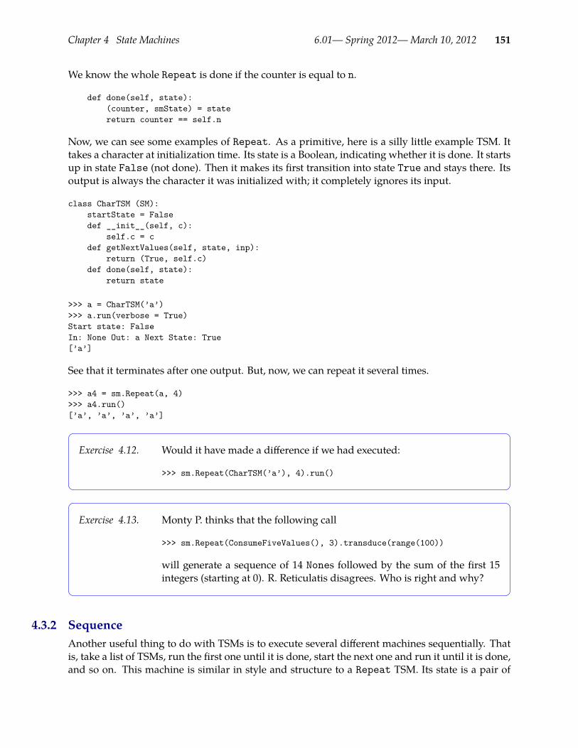
Chapter 4 State Machines 6.01— Spring 2012—March 10, 2012 151
We know the whole Repeat is done if the counter is equal to n.
def done(self, state):(counter, smState) = statereturn counter == self.n
Now, we can see some examples of Repeat. As a primitive, here is a silly little example TSM. Ittakes a character at initialization time. Its state is a Boolean, indicating whether it is done. It startsup in state False (not done). Then it makes its first transition into state True and stays there. Itsoutput is always the character it was initialized with; it completely ignores its input.
class CharTSM (SM):startState = Falsedef __init__(self, c):
self.c = cdef getNextValues(self, state, inp):
return (True, self.c)def done(self, state):
return state
>>> a = CharTSM(’a’)>>> a.run(verbose = True)Start state: FalseIn: None Out: a Next State: True[’a’]
See that it terminates after one output. But, now, we can repeat it several times.
>>> a4 = sm.Repeat(a, 4)>>> a4.run()[’a’, ’a’, ’a’, ’a’]
Exercise 4.12. Would it have made a difference if we had executed:
>>> sm.Repeat(CharTSM(’a’), 4).run()
Exercise 4.13. Monty P. thinks that the following call
>>> sm.Repeat(ConsumeFiveValues(), 3).transduce(range(100))
will generate a sequence of 14 Nones followed by the sum of the first 15integers (starting at 0). R. Reticulatis disagrees. Who is right and why?
4.3.2 SequenceAnother useful thing to do with TSMs is to execute several different machines sequentially. Thatis, take a list of TSMs, run the first one until it is done, start the next one and run it until it is done,and so on. This machine is similar in style and structure to a Repeat TSM. Its state is a pair of

Chapter 4 State Machines 6.01— Spring 2012—March 10, 2012 152
values: an index that says which of the constituent machines is currently being executed, and thestate of the current constituent.
Here is a Python class for creating a Sequence TSM. It takes as input a list of state machines; itremembers the machines and number of machines in the list.
class Sequence (SM):def __init__(self, smList):
self.smList = smListself.startState = (0, self.smList[0].startState)self.n = len(smList)
The initial state of this machine is the value 0 (because we start by executing the 0th constituentmachine on the list) and the initial state of that constituent machine.
The method for advancing is also similar that for Repeat. The only difference is that each time,we start the next machine in the list of machines, until we have finished executing the last one.
def advanceIfDone(self, counter, smState):while self.smList[counter].done(smState) and counter + 1 < self.n:
counter = counter + 1smState = self.smList[counter].startState
return (counter, smState)
To get the next state, we ask the current constituent machine for its next state, and then, if it isdone, advance the state to the next machine in the list that is not done when it wakes up. Theoutput of the composite machine is just the output of the current constituent.
def getNextValues(self, state, inp):(counter, smState) = state(smState, o) = self.smList[counter].getNextValues(smState, inp)(counter, smState) = self.advanceIfDone(counter, smState)return ((counter, smState), o)
We have constructed this machine so that it always advances past any constituent machine that isdone; if, in fact, the current constituent machine is done, then the whole machine is also done.
def done(self, state):(counter, smState) = statereturn self.smList[counter].done(smState)
We can make good use of the CharTSM to test our sequential combinator. First, we will try some-thing simple:
>>> m = sm.Sequence([CharTSM(’a’), CharTSM(’b’), CharTSM(’c’)])>>> m.run()Start state: (0, False)In: None Out: a Next State: (1, False)In: None Out: b Next State: (2, False)In: None Out: c Next State: (2, True)[’a’, ’b’, ’c’]
Even in a test case, there is something unsatisfying about all that repetitive typing required tomakeeach individual CharTSM. If we are repeating, we should abstract. So, we can write a function that
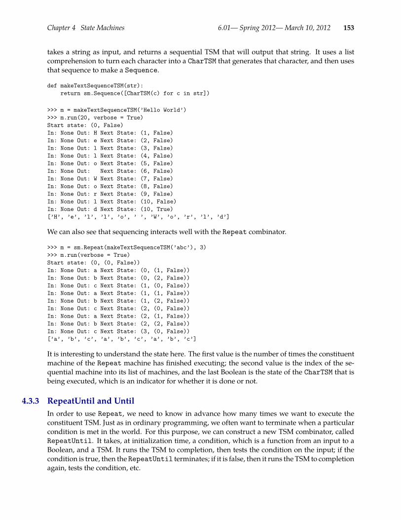
Chapter 4 State Machines 6.01— Spring 2012—March 10, 2012 153
takes a string as input, and returns a sequential TSM that will output that string. It uses a listcomprehension to turn each character into a CharTSM that generates that character, and then usesthat sequence to make a Sequence.
def makeTextSequenceTSM(str):return sm.Sequence([CharTSM(c) for c in str])
>>> m = makeTextSequenceTSM(’Hello World’)>>> m.run(20, verbose = True)Start state: (0, False)In: None Out: H Next State: (1, False)In: None Out: e Next State: (2, False)In: None Out: l Next State: (3, False)In: None Out: l Next State: (4, False)In: None Out: o Next State: (5, False)In: None Out: Next State: (6, False)In: None Out: W Next State: (7, False)In: None Out: o Next State: (8, False)In: None Out: r Next State: (9, False)In: None Out: l Next State: (10, False)In: None Out: d Next State: (10, True)[’H’, ’e’, ’l’, ’l’, ’o’, ’ ’, ’W’, ’o’, ’r’, ’l’, ’d’]
We can also see that sequencing interacts well with the Repeat combinator.
>>> m = sm.Repeat(makeTextSequenceTSM(’abc’), 3)>>> m.run(verbose = True)Start state: (0, (0, False))In: None Out: a Next State: (0, (1, False))In: None Out: b Next State: (0, (2, False))In: None Out: c Next State: (1, (0, False))In: None Out: a Next State: (1, (1, False))In: None Out: b Next State: (1, (2, False))In: None Out: c Next State: (2, (0, False))In: None Out: a Next State: (2, (1, False))In: None Out: b Next State: (2, (2, False))In: None Out: c Next State: (3, (0, False))[’a’, ’b’, ’c’, ’a’, ’b’, ’c’, ’a’, ’b’, ’c’]
It is interesting to understand the state here. The first value is the number of times the constituentmachine of the Repeat machine has finished executing; the second value is the index of the se-quential machine into its list of machines, and the last Boolean is the state of the CharTSM that isbeing executed, which is an indicator for whether it is done or not.
4.3.3 RepeatUntil and UntilIn order to use Repeat, we need to know in advance how many times we want to execute theconstituent TSM. Just as in ordinary programming, we often want to terminate when a particularcondition is met in the world. For this purpose, we can construct a new TSM combinator, calledRepeatUntil. It takes, at initialization time, a condition, which is a function from an input to aBoolean, and a TSM. It runs the TSM to completion, then tests the condition on the input; if thecondition is true, then the RepeatUntil terminates; if it is false, then it runs the TSM to completionagain, tests the condition, etc.
Chapter 4 State Machines 6.01— Spring 2012—March 10, 2012 154
Here is the Python code for implementing RepeatUntil. The state of this machine has two parts:a Boolean indicating whether the condition is true, and the state of the constituent machine.
class RepeatUntil (SM):def __init__(self, condition, sm):
self.sm = smself.condition = conditionself.startState = (False, self.sm.startState)
def getNextValues(self, state, inp):(condTrue, smState) = state(smState, o) = self.sm.getNextValues(smState, inp)condTrue = self.condition(inp)if self.sm.done(smState) and not condTrue:
smState = self.sm.getStartState()return ((condTrue, smState), o)
def done(self, state):(condTrue, smState) = statereturn self.sm.done(smState) and condTrue
One important thing to note is that, in the RepeatUntil TSM the condition is only evaluatedwhen the constituent TSM is done. This is appropriate in some situations; but in other cases, wewould like to terminate the execution of a TSM if a condition becomes true at any single step ofthe machine. We could easily implement something like this in any particular case, by defininga special-purpose TSM class that has a done method that tests the termination condition. But,because this structure is generally useful, we can define a general-purpose combinator, called Un-til. This combinator also takes a condition and a constituent machine. It simply executes theconstituent machine, and terminates either when the condition becomes true, or when the con-stituent machine terminates. As before, the state includes the value of the condition on the lastinput and the state of the constituent machine.
Note that this machine will never execute the constituent machine more than once; it will eitherrun it once to completion (if the condition never becomes true), or terminate it early.
Here are some examples of using RepeatUntil and Until. First, we run the ConsumeFiveVal-uesmachine until the input is greater than 10. Because it only tests the condition when Consume-FiveValues is done, and the condition only becomes true on the 11th step, the ConsumeFive-Valuesmachine is run to completion three times.
def greaterThan10 (x):return x > 10
>>> m = sm.RepeatUntil(greaterThan10, ConsumeFiveValues())>>> m.transduce(range(20), verbose = True)Start state: (0, 0)In: 0 Out: None Next State: (1, 0)In: 1 Out: None Next State: (2, 1)In: 2 Out: None Next State: (3, 3)In: 3 Out: None Next State: (4, 6)In: 4 Out: 10 Next State: (0, 0)In: 5 Out: None Next State: (1, 5)In: 6 Out: None Next State: (2, 11)In: 7 Out: None Next State: (3, 18)
Chapter 4 State Machines 6.01— Spring 2012—March 10, 2012 155
In: 8 Out: None Next State: (4, 26)In: 9 Out: 35 Next State: (0, 0)In: 10 Out: None Next State: (1, 10)In: 11 Out: None Next State: (2, 21)In: 12 Out: None Next State: (3, 33)In: 13 Out: None Next State: (4, 46)In: 14 Out: 60 Next State: (5, 60)[None, None, None, None, 10, None, None, None, None, 35, None, None, None, None, 60]
If we do Until on the basic ConsumeFiveValuesmachine, then it just runs ConsumeFiveValuesuntil it terminates normally, because the condition never becomes true during this time.
>>> m = sm.Until(greaterThan10, ConsumeFiveValues())>>> m.transduce(range(20), verbose = True)Start state: (False, (0, 0))In: 0 Out: None Next State: (False, (1, 0))In: 1 Out: None Next State: (False, (2, 1))In: 2 Out: None Next State: (False, (3, 3))In: 3 Out: None Next State: (False, (4, 6))In: 4 Out: 10 Next State: (False, (5, 10))[None, None, None, None, 10]
However, if we change the termination condition, the executionwill be terminated early. Note thatwe can use a lambda expression directly as an argument; sometimes this is actually clearer thandefining a function with def, but it is fine to do it either way.
>>> m = sm.Until(lambda x: x == 2, ConsumeFiveValues())>>> m.transduce(range(20), verbose = True)Start state: (False, (0, 0))In: 0 Out: None Next State: (False, (1, 0))In: 1 Out: None Next State: (False, (2, 1))In: 2 Out: None Next State: (True, (3, 3))[None, None, None]
If we actuallywant to keep repeating ConsumeFiveValues()until the condition becomes true, wecan combine Until with Repeat. Now, we see that it executes the constituent machine multipletimes, but terminates as soon as the condition is satisfied.
>>> m = sm.Until(greaterThan10, sm.Repeat(ConsumeFiveValues()))>>> m.transduce(range(20), verbose = True)Start state: (False, (0, (0, 0)))In: 0 Out: None Next State: (False, (0, (1, 0)))In: 1 Out: None Next State: (False, (0, (2, 1)))In: 2 Out: None Next State: (False, (0, (3, 3)))In: 3 Out: None Next State: (False, (0, (4, 6)))In: 4 Out: 10 Next State: (False, (1, (0, 0)))In: 5 Out: None Next State: (False, (1, (1, 5)))In: 6 Out: None Next State: (False, (1, (2, 11)))In: 7 Out: None Next State: (False, (1, (3, 18)))In: 8 Out: None Next State: (False, (1, (4, 26)))In: 9 Out: 35 Next State: (False, (2, (0, 0)))In: 10 Out: None Next State: (False, (2, (1, 10)))In: 11 Out: None Next State: (True, (2, (2, 21)))[None, None, None, None, 10, None, None, None, None, 35, None, None]

Chapter 4 State Machines 6.01— Spring 2012—March 10, 2012 156
4.4 Using a state machine to control the robotThis section gives an overview of how to control the robot with a state machine. For a muchmore detailed description, see the Infrastructure Guide, which documents the io and utilmodulesin detail. The io module provides procedures and methods for interacting with the robot; theutilmodule provides procedures and methods for doing computations that are generally useful(manipulating angles, dealing with coordinate frames, etc.)We can implement a robot controller as a state machine whose inputs are instances of classio.SensorInput, and whose outputs are instances of class io.Action.Here is Python code for a brain that is controlled by themost basic of statemachines. Thismachinealways emits the default action, io.Action(), which sets all of the output values to zero. Whenthe brain is set up, we create a “behavior”, which is a name we will use for a state machine thattransduces a stream of io.SensorInputs to a stream of io.Actions. Finally, we ask the behaviorto start.Then, all we do in the stepmethod of the robot is:• Read the sensors, by calling io.SensorInput() to get an instance that contains sonar andodometry readings;• Feed that sensor input to the brain state machine, by calling its stepmethod with that as input;and• Take the io.Action that is generated by the brain as output, and call its execute method,which causes it to actually send motor commands to the robot.
You can set the verbose flag to True if you want to see a lot of output on each step for debugging.Inside a Soar brain, we have access to an object robot, which persists during the entire executionof the brain, and gives us a place to store important objects (like the state machine that will bedoing all the work).
import smimport io
class StopSM(sm.SM):def getNextValues(self, state, inp):
return (None, io.Action())
def setup():robot.behavior = StopSM()robot.behavior.start()
def step():robot.behavior.step(io.SensorInput(), verbose = False).execute()
In the following sections we will develop two simple machines for controlling a robot to move afixed distance or turn through a fixed angle. Then we will put them together and explore why itcan be useful to have the starting state of a machine depend on the input.
4.4.1 RotateImagine that wewant the robot to rotate a fixed angle, say 90 degrees, to the left of where it is whenit starts to run a behavior. We can use the robot’s odometry to measure approximately where it is,

Chapter 4 State Machines 6.01— Spring 2012—March 10, 2012 157
in an arbitrary coordinate frame; but to know how much it has moved since we started, we haveto store some information in the state.
Here is a class that defines a Rotate state machine. It takes, at initialization time, a desired changein heading.
class RotateTSM (SM):rotationalGain = 3.0angleEpsilon = 0.01startState = ’start’
def __init__(self, headingDelta):self.headingDelta = headingDelta
When it is time to start this machine, we would like to look at the robot’s current heading (theta),add the desired change in heading, and store the result in our state as the desired heading. Then,in order to test whether the behavior is done, we want to see whether the current heading is closeenough to the desired heading. Because the donemethod does not have access to the input of themachine (it is a property only of states), we need to include the current theta in the state. So, thestate of the machine is (thetaDesired, thetaLast).
Thus, the getNextValuesmethod looks at the state; if it is the special symbol ’start’, it meansthat the machine has not previously had a chance to observe the input and see what its currentheading is, so it computes the desired heading (by adding the desired change to the current head-ing, and then calling a utility procedure to be sure the resulting angle is between plus and minusπ), and returns it and the current heading. Otherwise, we keep the thetaDesired componentof the state, and just get a new value of theta out of the input. We generate an action with arotational velocity that will rotate toward the desired heading with velocity proportional to themagnitude of the angular error.
def getNextValues(self, state, inp):currentTheta = inp.odometry.thetaif state == ’start’:
thetaDesired = \util.fixAnglePlusMinusPi(currentTheta + self.headingDelta)
else:(thetaDesired, thetaLast) = state
newState = (thetaDesired, currentTheta)action = io.Action(rvel = self.rotationalGain * \
util.fixAnglePlusMinusPi(thetaDesired - currentTheta))
return (newState, action)
Finally, we have to say which states are done. Clearly, the ’start’ state is not done; but we aredone if the most recent theta from the odometry is within some tolerance, self.angleEpsilon,of the desired heading.
def done(self, state):if state == ’start’:
return Falseelse:
(thetaDesired, thetaLast) = statereturn util.nearAngle(thetaDesired, thetaLast, self.angleEpsilon)
Chapter 4 State Machines 6.01— Spring 2012—March 10, 2012 158
Exercise 4.14. Change this machine so that it rotates through an angle, so you could giveit 2 pi or minus 2 pi to have it rotate all the way around.
4.4.2 ForwardMoving the robot forward a fixed distance is similar. In this case, we remember the robot’s xand y coordinates when it starts, and drive straight forward until the distance between the initialposition and the current position is close to the desired distance. The state of the machine is therobot’s starting position and its current position.
class ForwardTSM (SM):forwardGain = 1.0distTargetEpsilon = 0.01startState = ’start’
def __init__(self, delta):self.deltaDesired = delta
def getNextValues(self, state, inp):currentPos = inp.odometry.point()if state == ’start’:
print "Starting forward", self.deltaDesiredstartPos = currentPos
else:(startPos, lastPos) = state
newState = (startPos, currentPos)error = self.deltaDesired - startPos.distance(currentPos)action = io.Action(fvel = self.forwardGain * error)return (newState, action)
def done(self, state):if state == ’start’:
return Falseelse:
(startPos, lastPos) = statereturn util.within(startPos.distance(lastPos),
self.deltaDesired,self.distTargetEpsilon)
4.4.3 Square SpiralImagine we would like to have the robot drive in a square spiral, similar to the one shown infigure 4.11. One way to approach this problem is to make a “low-level” machine that can consumea goal point and the sensor input and drive (in the absence of obstacles) to the goal point; and thenmake a “high-level”machine that will keep track of wherewe are in the figure and feed goal pointsto the low-level machine.
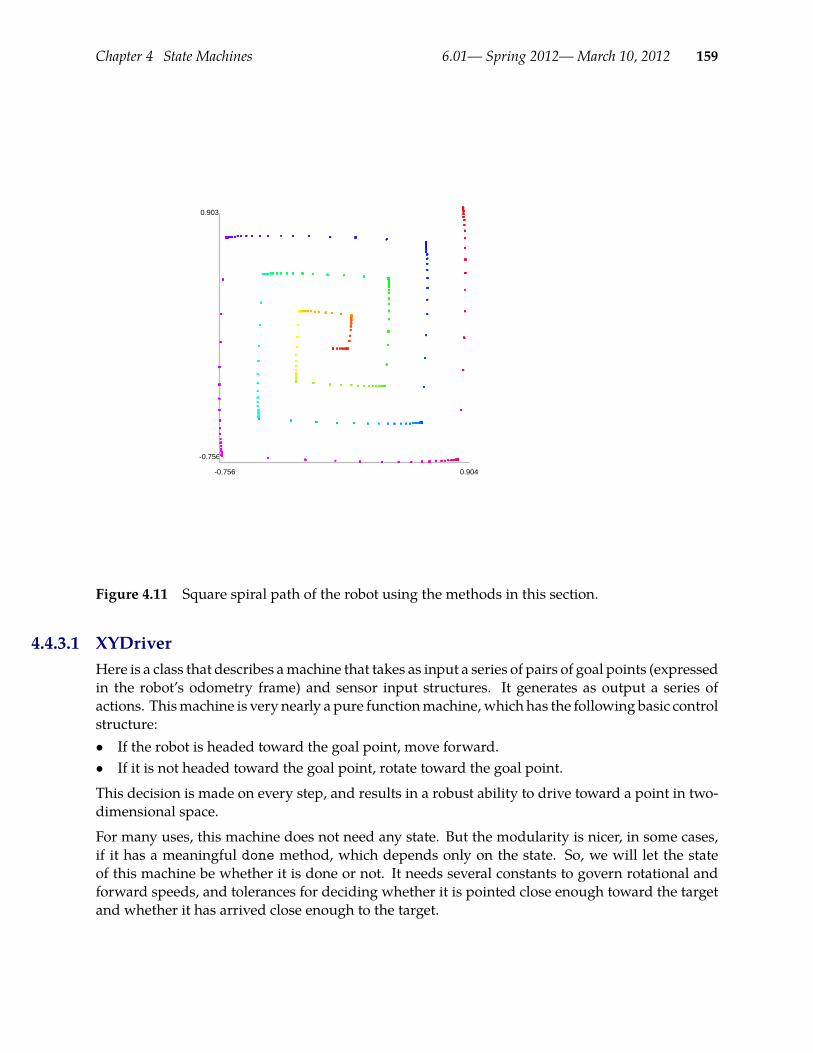
Chapter 4 State Machines 6.01— Spring 2012—March 10, 2012 159
-0.756 0.904
-0.756
0.903
Figure 4.11 Square spiral path of the robot using the methods in this section.
4.4.3.1 XYDriverHere is a class that describes amachine that takes as input a series of pairs of goal points (expressedin the robot’s odometry frame) and sensor input structures. It generates as output a series ofactions. Thismachine is very nearly a pure functionmachine, which has the following basic controlstructure:• If the robot is headed toward the goal point, move forward.• If it is not headed toward the goal point, rotate toward the goal point.
This decision is made on every step, and results in a robust ability to drive toward a point in two-dimensional space.
For many uses, this machine does not need any state. But the modularity is nicer, in some cases,if it has a meaningful done method, which depends only on the state. So, we will let the stateof this machine be whether it is done or not. It needs several constants to govern rotational andforward speeds, and tolerances for deciding whether it is pointed close enough toward the targetand whether it has arrived close enough to the target.

Chapter 4 State Machines 6.01— Spring 2012—March 10, 2012 160
class XYDriver(SM):forwardGain = 2.0rotationGain = 2.0angleEps = 0.05distEps = 0.02startState = False
The getNextValuesmethod embodies the control structure described above.
def getNextValues(self, state, inp):(goalPoint, sensors) = inprobotPose = sensors.odometryrobotPoint = robotPose.point()robotTheta = robotPose.theta
if goalPoint == None:return (True, io.Action())
headingTheta = robotPoint.angleTo(goalPoint)if util.nearAngle(robotTheta, headingTheta, self.angleEps):
# Pointing in the right direction, so move forwardr = robotPoint.distance(goalPoint)if r < self.distEps:
# We’re therereturn (True, io.Action())
else:return (False, io.Action(fvel = r * self.forwardGain))
else:# Rotate to point toward goalheadingError = util.fixAnglePlusMinusPi(\
headingTheta - robotTheta)return (False, io.Action(rvel = headingError * self.rotationGain))
The state of the machine is just a boolean indicating whether we are done.
def done(self, state):return state
4.4.3.2 Cascade approachWe make a spiral by building a machine that takes SensorInput objects as input and generatespairs of subgoals and sensorinputs; such a machine can be cascaded with XYDriver to generate aspiral.
Our implementation of this is a class called SpyroGyra. It takes the increment (amount that eachnew side is larger than the previous) at initialization time. Its state consists of three components:• direction: one of ’north’, ’south’, ’east’, or ’west’, indicating which way the robot is traveling• length: length in meters of the current line segment being followed• subGoal: the point in the robot’s odometry frame that defines the end of the current line seg-
ment
It requires a tolerance to decide when the current subgoal point has been reached.

Chapter 4 State Machines 6.01— Spring 2012—March 10, 2012 161
class SpyroGyra(SM):distEps = 0.02def __init__(self, incr):
self.incr = incrself.startState = (’south’, 0, None)
If the robot is close enough to the subgoal point, then it is time to change the state. We incrementthe side length, pick the next direction (counter clockwise around the cardinal compass directions),and compute the next subgoal point. The output is just the subgoal and the sensor input, whichis what the driver needs.
def getNextValues(self, state, inp):(direction, length, subGoal) = staterobotPose = inp.odometryrobotPoint = robotPose.point()if subGoal == None:
subGoal = robotPointif robotPoint.isNear(subGoal, self.distEps):
# Time to change statelength = length + self.incrif direction == ’east’:
direction = ’north’subGoal.y += length
elif direction == ’north’:direction = ’west’subGoal.x -= length
elif direction == ’west’:direction = ’south’subGoal.y -= length
else: # southdirection = ’east’subGoal.x += length
print ’new:’, direction, length, subGoalreturn ((direction, length, subGoal),
(subGoal, inp))
Finally, to make the spiral, we just cascade these two machines together.
def spiroFlow(incr):return sm.Cascade(SpyroGyra(incr), XYDriver())
Exercise 4.15. What explains the rounded sides of the path in figure 4.11?
4.5 Conclusion
State machinesState machines are such a general formalism, that a huge class of discrete-time systems can bedescribed as state machines. The system of defining primitive machines and combinations givesus one discipline for describing complex systems. It will turn out that there are some systems that

Chapter 4 State Machines 6.01— Spring 2012—March 10, 2012 162
are conveniently defined using this discipline, but that for other kinds of systems, other disciplineswould be more natural. As you encounter complex engineering problems, your job is to find thePCAP system that is appropriate for them, and if one does not exist already, invent one.
State machines are such a general class of systems that although it is a useful framework for im-plementing systems, we cannot generally analyze the behavior of state machines. That is, we can’tmake much in the way of generic predictions about their future behavior, except by running themto see what will happen.
In the next module, wewill look at a restricted class of state machines, whose state is representableas a bounded history of their previous states and previous inputs, and whose output is a linearfunction of those states and inputs. This is amuch smaller class of systems than all state machines,but it is nonetheless very powerful. The important lesson will be that restricting the form of themodels we are using will allow us to make stronger claims about their behavior.
Knuth on Elevator ControllersDonald E. Knuth is a computer scientist who is famous for, among other things, his series of textbooks (as wellas for TEX, the typesetting system we use to make all of our handouts), and a variety of other contributionsto theoretical computer science.
“It is perhaps significant to note that although the author had used the elevator system for yearsand thought he knew it well, it wasn’t until he attempted to write this section that he realized therewere quite a few facts about the elevator’s system of choosing directions that he did not know. Hewent back to experiment with the elevator six separate times, each time believing he had finallyachieved a complete understanding of its modus operandi. (Now he is reluctant to ride it for fearsome new facet of its operation will appear, contradicting the algorithms given.) We often fail torealize how little we know about a thing until we attempt to simulate it on a computer.”
The Art of Computer Programming, Donald E., Knuth, Vol 1. page 295. On the elevator system in theMathematics Building at Cal Tech. First published in 1968
4.6 Examples
4.6.1 Practice problem: ThingsConsider the following program
def thing(inputList):output = []i = 0for x in range(3):
y = 0while y < 100 and i < len(inputList):
y = y + inputList[i]output.append(y)i = i + 1
return output
A. What is the value of
thing([1, 2, 3, 100, 4, 9, 500, 51, -2, 57, 103, 1, 1, 1, 1, -10, 207, 3, 1])
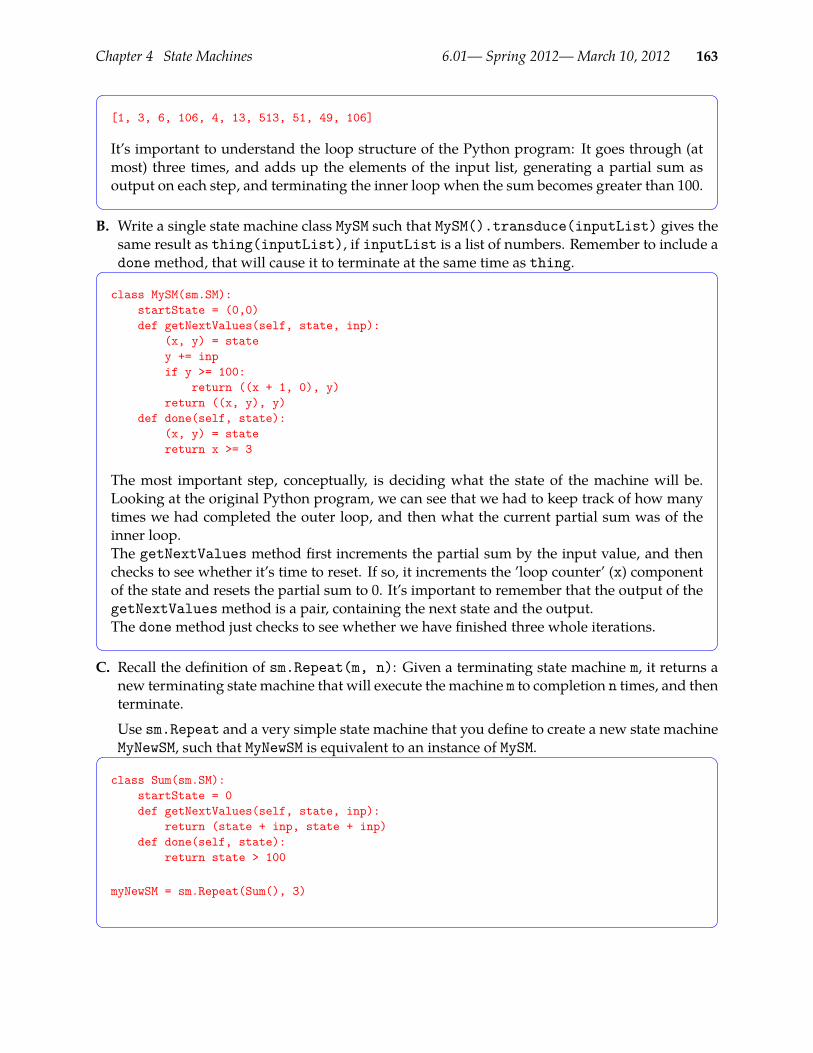
Chapter 4 State Machines 6.01— Spring 2012—March 10, 2012 163
[1, 3, 6, 106, 4, 13, 513, 51, 49, 106]
It’s important to understand the loop structure of the Python program: It goes through (atmost) three times, and adds up the elements of the input list, generating a partial sum asoutput on each step, and terminating the inner loop when the sum becomes greater than 100.
B. Write a single state machine class MySM such that MySM().transduce(inputList) gives thesame result as thing(inputList), if inputList is a list of numbers. Remember to include adonemethod, that will cause it to terminate at the same time as thing.
class MySM(sm.SM):startState = (0,0)def getNextValues(self, state, inp):
(x, y) = statey += inpif y >= 100:
return ((x + 1, 0), y)return ((x, y), y)
def done(self, state):(x, y) = statereturn x >= 3
The most important step, conceptually, is deciding what the state of the machine will be.Looking at the original Python program, we can see that we had to keep track of how manytimes we had completed the outer loop, and then what the current partial sum was of theinner loop.The getNextValues method first increments the partial sum by the input value, and thenchecks to see whether it’s time to reset. If so, it increments the ’loop counter’ (x) componentof the state and resets the partial sum to 0. It’s important to remember that the output of thegetNextValuesmethod is a pair, containing the next state and the output.The donemethod just checks to see whether we have finished three whole iterations.
C. Recall the definition of sm.Repeat(m, n): Given a terminating state machine m, it returns anew terminating state machine that will execute the machine m to completion n times, and thenterminate.
Use sm.Repeat and a very simple state machine that you define to create a new state machineMyNewSM, such that MyNewSM is equivalent to an instance of MySM.
class Sum(sm.SM):startState = 0def getNextValues(self, state, inp):
return (state + inp, state + inp)def done(self, state):
return state > 100
myNewSM = sm.Repeat(Sum(), 3)

Chapter 4 State Machines 6.01— Spring 2012—March 10, 2012 164
4.6.2 Practice problem: Inheritance and State MachinesRecall that we have defined a Python class sm.SM to represent state machines. Here we consider aspecial type of state machine, whose states are always integers that start at 0 and increment by 1 oneach transition. We can represent this new type of state machines as a Python subclass of sm.SMcalled CountingStateMachine.
We wish to use the CountingStateMachine class to define new subclasses that each provide asingle new method getOutput(self, state, inp) which returns just the output for that stateand input; the CountingStateMachinewill take care of managing and incrementing the state, soits subclasses don’t have to worry about it.
Here is an example of a subclass of CountingStateMachine.
class CountMod5(CountingStateMachine):def getOutput(self, state, inp):
return state % 5
Instances of CountMod5 generate output sequences of the form 0, 1, 2, 3, 4, 0, 1, 2, 3,4, 0, . . ..
4.6.2.1 Part a.Define the CountingStateMachine class. Since CountingStateMachine is a subclass of sm.SM,you will have to provide definitions of the startState instance variable and getNextValuesmethod, just as we have done for other state machines. You can assume that every subclass ofCountingStateMachinewill provide an appropriate getOutputmethod.
class CountingStateMachine(sm.SM):def __init__(self):
self.startState = 0def getNextValues(self, state, inp):
return(state + 1, self.getOutput(state, inp))
4.6.2.2 Part b.Define a subclass of CountingStateMachine called AlternateZeros. Instances of Alter-nateZeros should be state machines for which, on even steps, the output is the same as the input,and on odd steps, the output is 0. That is, given inputs, i0, i1, i2, i3, . . ., they generate outputs,i0, 0, i2, 0, . . ..
class AlternateZeros(CountingStateMachine):def getOutput(self, state, inp):
if not state % 2:return inp
return 0

Chapter 5 Signals and Systems 6.01— Spring 2012—March 10, 2012 165
Chapter 5Signals and Systems
Imagine that you are asked to design a system to steer a car straight down the middle of a lane.It seems easy, right? You can figure out some way to sense the position of the car within its lane.Then, if the car is right of center, turn the steering wheel to the left. As the car moves so that itis less to the right, turn the steering wheel less to the left. If it is left of center, turn the steeringwheel to the right. This sort of proportional controller works well for many applications – but notfor steering, as can be seen below.
steer left
steer left
straight ahead?
steer right
steer right
steer right
straight ahead?
Figure 5.1 Simple (but poor) algorithm for steering: steer to the left in proportion to how far thecar is to the right, and vice versa.
It is relatively easy to describe better algorithms in terms that humans would understand: e.g.,Stop turning back and forth! It is not so easy to specify exactly what one might mean by that, in away that it could be automated.
In this chapter, we will develop a Signals and Systems framework to facilitate reasoning about thedynamic behaviors of systems. This framework will enable construction of simple mathematicalmodels that are useful in both analysis and design of a wide range of systems, including the car-steering system.
5.1 The signals and systems abstractionTo think about dynamic behaviors of systems, we need to think not only about how to describethe system but also about how to describe the signals that characterize the inputs and outputs ofthe system, as illustrated below.
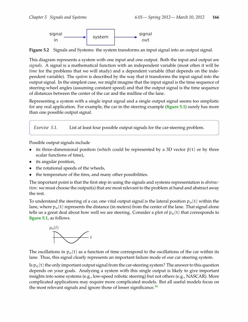
Chapter 5 Signals and Systems 6.01— Spring 2012—March 10, 2012 166
systemsignal
in
signal
out
Figure 5.2 Signals and Systems: the system transforms an input signal into an output signal.
This diagram represents a system with one input and one output. Both the input and output aresignals. A signal is a mathematical function with an independent variable (most often it will betime for the problems that we will study) and a dependent variable (that depends on the inde-pendent variable). The system is described by the way that it transforms the input signal into theoutput signal. In the simplest case, we might imagine that the input signal is the time sequence ofsteering-wheel angles (assuming constant speed) and that the output signal is the time sequenceof distances between the center of the car and the midline of the lane.
Representing a system with a single input signal and a single output signal seems too simplisticfor any real application. For example, the car in the steering example (figure 5.1) surely has morethan one possible output signal.
Exercise 5.1. List at least four possible output signals for the car-steering problem.
Possible output signals include• its three-dimensional position (which could be represented by a 3D vector p(t) or by three
scalar functions of time),• its angular position,• the rotational speeds of the wheels,• the temperature of the tires, and many other possibilities.
The important point is that the first step in using the signals and systems representation is abstrac-tion: wemust choose the output(s) that aremost relevant to the problem at hand and abstract awaythe rest.
To understand the steering of a car, one vital output signal is the lateral position po(t) within thelane, where po(t) represents the distance (in meters) from the center of the lane. That signal alonetells us a great deal about how well we are steering. Consider a plot of po(t) that corresponds tofigure 5.1, as follows.
po(t)
t
The oscillations in po(t) as a function of time correspond to the oscillations of the car within itslane. Thus, this signal clearly represents an important failure mode of our car steering system.
Ispo(t) the only important output signal from the car-steering system? The answer to this questiondepends on your goals. Analyzing a system with this single output is likely to give importantinsights into some systems (e.g., low-speed robotic steering) but not others (e.g., NASCAR). Morecomplicated applications may require more complicated models. But all useful models focus onthe most relevant signals and ignore those of lesser significance.34
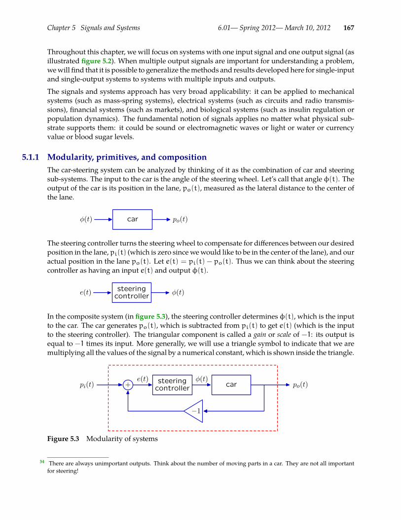
Chapter 5 Signals and Systems 6.01— Spring 2012—March 10, 2012 167
Throughout this chapter, we will focus on systems with one input signal and one output signal (asillustrated figure 5.2). When multiple output signals are important for understanding a problem,wewill find that it is possible to generalize themethods and results developed here for single-inputand single-output systems to systems with multiple inputs and outputs.
The signals and systems approach has very broad applicability: it can be applied to mechanicalsystems (such as mass-spring systems), electrical systems (such as circuits and radio transmis-sions), financial systems (such as markets), and biological systems (such as insulin regulation orpopulation dynamics). The fundamental notion of signals applies no matter what physical sub-strate supports them: it could be sound or electromagnetic waves or light or water or currencyvalue or blood sugar levels.
5.1.1 Modularity, primitives, and compositionThe car-steering system can be analyzed by thinking of it as the combination of car and steeringsub-systems. The input to the car is the angle of the steering wheel. Let’s call that angle φ(t). Theoutput of the car is its position in the lane, po(t), measured as the lateral distance to the center ofthe lane.
carφ(t) po(t)
The steering controller turns the steeringwheel to compensate for differences between our desiredposition in the lane, pi(t) (which is zero sincewewould like to be in the center of the lane), and ouractual position in the lane po(t). Let e(t) = pi(t) − po(t). Thus we can think about the steeringcontroller as having an input e(t) and output φ(t).
steeringcontrollere(t) φ(t)
In the composite system (in figure 5.3), the steering controller determines φ(t), which is the inputto the car. The car generates po(t), which is subtracted from pi(t) to get e(t) (which is the inputto the steering controller). The triangular component is called a gain or scale of −1: its output isequal to −1 times its input. More generally, we will use a triangle symbol to indicate that we aremultiplying all the values of the signal by a numerical constant, which is shown inside the triangle.
+ car
−1
steeringcontroller
φ(t)e(t)pi(t) po(t)
Figure 5.3 Modularity of systems
There are always unimportant outputs. Think about the number of moving parts in a car. They are not all important34
for steering!

Chapter 5 Signals and Systems 6.01— Spring 2012—March 10, 2012 168
Thedashed-red box infigure 5.3 illustratesmodularity of the signals and systems abstraction. Threesingle-input, single-output sub-systems (steering controller, car, and inverter) and an adder (twoinputs and 1 output) are combined to generate a new single-input (pi(t)), single-output (po(t))system. By abstraction, we could treat this new system as a primitive (represented by a single-input single-output box) and combine it with other subsystems to create a new, more complex,system. A principal goal of this chapter is to develop methods of analysis for the sub-systems thatcan be combined to analyze the overall system.
5.1.2 Discrete-time signals and systemsThis chapter focuses on signals whose independent variables are discrete (e.g., take on only inte-ger values). Some such signals are found in nature. For example, the primary structure of DNAis described by a sequence of base-pairs. However, we are primarily interested in discrete-timesignals, not so much because they are found in nature, but because they are found in computers.Even though we focus on interactions with the real world, these interactions will primarily occurat discrete instants of time. For example, the difference between our desired position pi(t) and ouractual position po(t) is an error signal e(t), which is a function of continuous time t. If the con-troller only observes this signal at regular sampling intervals T , then its input could be regarded asa sequence of values x[n] that is indexed by the integer n. The relation between the discrete-timesequence x[n] (note square brackets) and the continuous signal x(t) (note round brackets) is givenby
x[n] = x(nT) ,
which we call the sampling relation. Sampling converts a signal of continuous domain to one ofdiscrete domain.
While our primary focus will be on time signals, sampling works equally well in other domains.For example, images are typically represented as arrays of pixels accessed by integer-valued rowsand columns, rather than as continuous brightness fields, indexed by real-valued spatial coordi-nates.
If the car-steering problem in figure 5.1 were modeled in discrete time, we could describe thesystemwith a diagram that is very similar to the continuous-time diagram in figure 5.3. However,only discrete time instants are considered
+ car
−1
steeringcontroller
φ[n]e[n]pi[n] po[n]
and the output position is now only defined at discrete times, as shown below.
po[n]
n
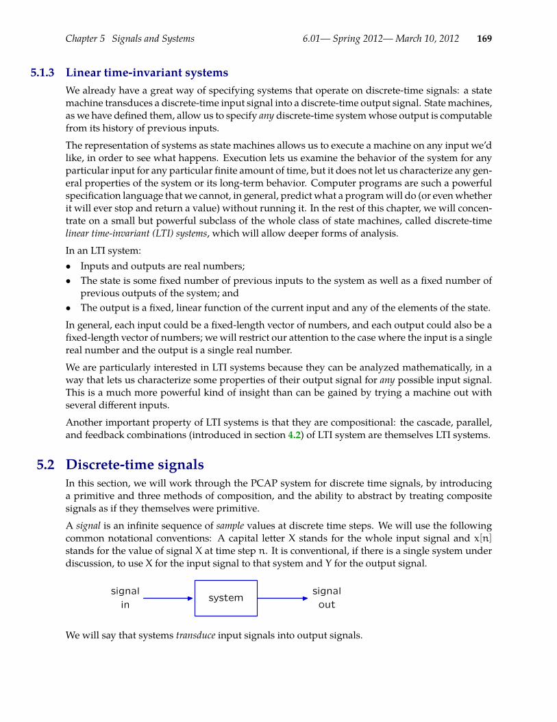
Chapter 5 Signals and Systems 6.01— Spring 2012—March 10, 2012 169
5.1.3 Linear time-invariant systemsWe already have a great way of specifying systems that operate on discrete-time signals: a statemachine transduces a discrete-time input signal into a discrete-time output signal. Statemachines,as we have defined them, allow us to specify any discrete-time systemwhose output is computablefrom its history of previous inputs.
The representation of systems as state machines allows us to execute a machine on any input we’dlike, in order to see what happens. Execution lets us examine the behavior of the system for anyparticular input for any particular finite amount of time, but it does not let us characterize any gen-eral properties of the system or its long-term behavior. Computer programs are such a powerfulspecification language that we cannot, in general, predict what a programwill do (or evenwhetherit will ever stop and return a value) without running it. In the rest of this chapter, we will concen-trate on a small but powerful subclass of the whole class of state machines, called discrete-timelinear time-invariant (LTI) systems, which will allow deeper forms of analysis.
In an LTI system:• Inputs and outputs are real numbers;• The state is some fixed number of previous inputs to the system as well as a fixed number of
previous outputs of the system; and• The output is a fixed, linear function of the current input and any of the elements of the state.
In general, each input could be a fixed-length vector of numbers, and each output could also be afixed-length vector of numbers; we will restrict our attention to the case where the input is a singlereal number and the output is a single real number.
We are particularly interested in LTI systems because they can be analyzed mathematically, in away that lets us characterize some properties of their output signal for any possible input signal.This is a much more powerful kind of insight than can be gained by trying a machine out withseveral different inputs.
Another important property of LTI systems is that they are compositional: the cascade, parallel,and feedback combinations (introduced in section 4.2) of LTI system are themselves LTI systems.
5.2 Discrete-time signalsIn this section, we will work through the PCAP system for discrete time signals, by introducinga primitive and three methods of composition, and the ability to abstract by treating compositesignals as if they themselves were primitive.
A signal is an infinite sequence of sample values at discrete time steps. We will use the followingcommon notational conventions: A capital letter X stands for the whole input signal and x[n]stands for the value of signal X at time step n. It is conventional, if there is a single system underdiscussion, to use X for the input signal to that system and Y for the output signal.
systemsignal
in
signal
out
We will say that systems transduce input signals into output signals.
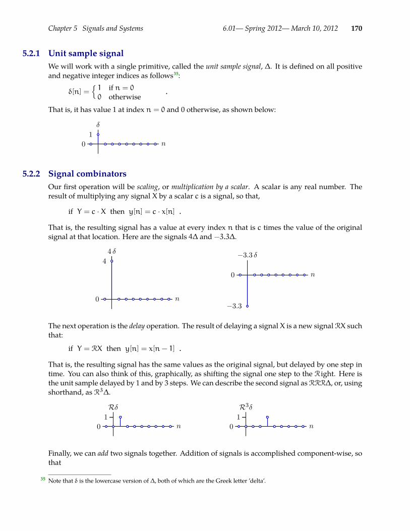
Chapter 5 Signals and Systems 6.01— Spring 2012—March 10, 2012 170
5.2.1 Unit sample signalWe will work with a single primitive, called the unit sample signal, ∆. It is defined on all positiveand negative integer indices as follows35:
δ[n] =1 if n = 00 otherwise
.
That is, it has value 1 at index n = 0 and 0 otherwise, as shown below:
n
δ
10
5.2.2 Signal combinatorsOur first operation will be scaling, or multiplication by a scalar. A scalar is any real number. Theresult of multiplying any signal X by a scalar c is a signal, so that,
if Y = c · X then y[n] = c · x[n] .
That is, the resulting signal has a value at every index n that is c times the value of the originalsignal at that location. Here are the signals 4∆ and −3.3∆.
n
4 δ4
0
n
−3.3 δ
−3.3
0
The next operation is the delay operation. The result of delaying a signal X is a new signalRX suchthat:
if Y = RX then y[n] = x[n− 1] .
That is, the resulting signal has the same values as the original signal, but delayed by one step intime. You can also think of this, graphically, as shifting the signal one step to the R ight. Here isthe unit sample delayed by 1 and by 3 steps. We can describe the second signal asRRR∆, or, usingshorthand, as R3∆.
n
Rδ1
0 n
R3δ1
0
Finally, we can add two signals together. Addition of signals is accomplished component-wise, sothat
Note that δ is the lowercase version of ∆, both of which are the Greek letter ’delta’.35

Chapter 5 Signals and Systems 6.01— Spring 2012—March 10, 2012 171
if Y = X1 + X2 then y[n] = x1[n] + x2[n] .
That is, the value of the composite signal at stepn is the sumof the values of the component signals.Here are some new signals constructed by summing, scaling, and delaying the unit sample.
n
δ +R2δ +R4δ
10
n
3δ + 4Rδ − 2R2δ
4
0
Note that, because each of our operations returns a signal, we can use their results again as ele-ments in new combinations, showing that our system has true compositionality. In addition, wecan abstract, by naming signals. So, for example, we might define Y = 3∆ + 4R∆ − 2R2∆, andthen make a new signal Z = Y + 0.3RY, which would look like this:
n
Z = Y + 0.3RY5
0
Be sure you understand how the heights of the spikes are determined by the definition of Z.
Exercise 5.2. Draw a picture of samples −1 through 4 of Y − RY.
It is important to remember that, because signals are infinite objects, these combination operationsare abstract mathematical operations. You could never somehow ’make’ a new signal by calculat-ing its value at every index. It is possible, however, to calculate the value at any particular index,as it is required.
AdvancingIf we allow ourselves one more operation, that of ’advancing’ the signal one step (just likedelaying, but in the other direction, written L for left-shift), then any signal can be com-posed from the unit sample, using a (possibly infinite) number of these operations. We candemonstrate this claim by construction: to define a signal V with value vn at index n, for any setof integer n, we simply set
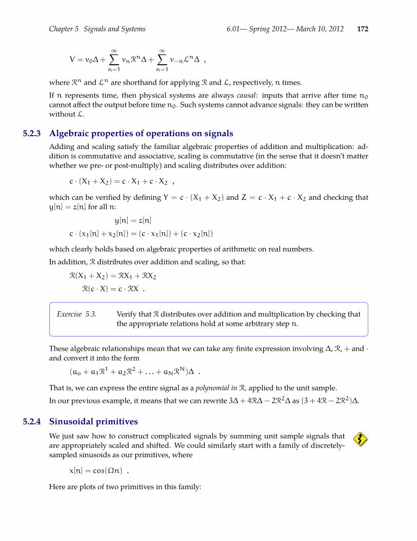
Chapter 5 Signals and Systems 6.01— Spring 2012—March 10, 2012 172
V = v0∆+
∞∑n=1
vnRn∆+
∞∑n=1
v−nLn∆ ,
where Rn and Ln are shorthand for applying R and L, respectively, n times.
If n represents time, then physical systems are always causal: inputs that arrive after time n0cannot affect the output before time n0. Such systems cannot advance signals: they can be writtenwithout L.
5.2.3 Algebraic properties of operations on signalsAdding and scaling satisfy the familiar algebraic properties of addition and multiplication: ad-dition is commutative and associative, scaling is commutative (in the sense that it doesn’t matterwhether we pre- or post-multiply) and scaling distributes over addition:
c · (X1 + X2) = c · X1 + c · X2 ,
which can be verified by defining Y = c · (X1 + X2) and Z = c · X1 + c · X2 and checking thaty[n] = z[n] for all n:
y[n] = z[n]
c · (x1[n] + x2[n]) = (c · x1[n]) + (c · x2[n])
which clearly holds based on algebraic properties of arithmetic on real numbers.
In addition, R distributes over addition and scaling, so that:
R(X1 + X2) = RX1 + RX2
R(c · X) = c · RX .
Exercise 5.3. Verify that R distributes over addition and multiplication by checking thatthe appropriate relations hold at some arbitrary step n.
These algebraic relationships mean that we can take any finite expression involving ∆, R, + and ·and convert it into the form
(ao + a1R1 + a2R
2 + . . .+ aNRN)∆ .
That is, we can express the entire signal as a polynomial in R, applied to the unit sample.
In our previous example, it means that we can rewrite 3∆+ 4R∆− 2R2∆ as (3+ 4R− 2R2)∆.
5.2.4 Sinusoidal primitivesWe just saw how to construct complicated signals by summing unit sample signals thatare appropriately scaled and shifted. We could similarly start with a family of discretely-sampled sinusoids as our primitives, where
x[n] = cos(Ωn) .
Here are plots of two primitives in this family:

Chapter 5 Signals and Systems 6.01— Spring 2012—March 10, 2012 173
cos(0.2n) cos(1.0n)
The second plot may seem confusing, but it is just a sparsely sampled sinusoid. Note that signalsconstructed from even a single sinusoid have non-zero values defined at an infinity of steps; thisis in contrast to signals constructed from a finite sum of scaled and shifted unit samples.
Exercise 5.4. If x[n] = cos(0.2n), what would be the values of RX at steps −3 and 5?
Here are two sinusoids and their sum, made as follows:
s1[n] = cos(0.2n− π/2)
S2 = R10S1
S3 = S1 + S2
The blue line is the S1, the green line is the same signal, delayed by 10, which is S2, and the redline is their sum.
1.099
-1.090 100
0
5.3 Feedforward systemsWewill start by looking at a subclass of discrete-time LTI system, which are exactly those that canbe described as performing some combination of scaling, delay, and addition operations on theinput signal. We will develop several ways of representing such systems, and see how to combinethem to get more complex systems in this same class.
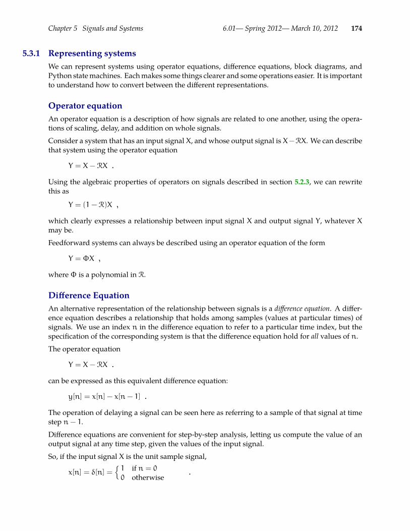
Chapter 5 Signals and Systems 6.01— Spring 2012—March 10, 2012 174
5.3.1 Representing systemsWe can represent systems using operator equations, difference equations, block diagrams, andPython statemachines. Eachmakes some things clearer and some operations easier. It is importantto understand how to convert between the different representations.
Operator equationAn operator equation is a description of how signals are related to one another, using the opera-tions of scaling, delay, and addition on whole signals.
Consider a system that has an input signal X, and whose output signal is X−RX. We can describethat system using the operator equation
Y = X− RX .
Using the algebraic properties of operators on signals described in section 5.2.3, we can rewritethis as
Y = (1− R)X ,
which clearly expresses a relationship between input signal X and output signal Y, whatever Xmay be.
Feedforward systems can always be described using an operator equation of the form
Y = ΦX ,
whereΦ is a polynomial in R.
Difference EquationAn alternative representation of the relationship between signals is a difference equation. A differ-ence equation describes a relationship that holds among samples (values at particular times) ofsignals. We use an index n in the difference equation to refer to a particular time index, but thespecification of the corresponding system is that the difference equation hold for all values of n.
The operator equation
Y = X− RX .
can be expressed as this equivalent difference equation:
y[n] = x[n] − x[n− 1] .
The operation of delaying a signal can be seen here as referring to a sample of that signal at timestep n− 1.
Difference equations are convenient for step-by-step analysis, letting us compute the value of anoutput signal at any time step, given the values of the input signal.
So, if the input signal X is the unit sample signal,
x[n] = δ[n] =1 if n = 00 otherwise
.
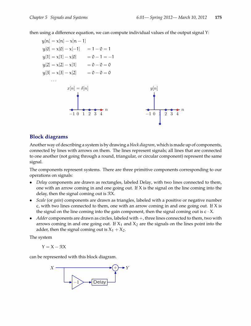
Chapter 5 Signals and Systems 6.01— Spring 2012—March 10, 2012 175
then using a difference equation, we can compute individual values of the output signal Y:
y[n] = x[n] − x[n− 1]
y[0] = x[0] − x[−1] = 1− 0 = 1
y[1] = x[1] − x[0] = 0− 1 = −1
y[2] = x[2] − x[1] = 0− 0 = 0
y[3] = x[3] − x[2] = 0− 0 = 0
· · ·
−1 0 1 2 3 4n
x[n] = δ[n]
−1 0 1 2 3 4n
y[n]
Block diagramsAnotherway of describing a system is bydrawing a block diagram, which ismadeupof components,connected by lines with arrows on them. The lines represent signals; all lines that are connectedto one another (not going through a round, triangular, or circular component) represent the samesignal.
The components represent systems. There are three primitive components corresponding to ouroperations on signals:• Delay components are drawn as rectangles, labeled Delay, with two lines connected to them,
one with an arrow coming in and one going out. If X is the signal on the line coming into thedelay, then the signal coming out is RX.
• Scale (or gain) components are drawn as triangles, labeled with a positive or negative numberc, with two lines connected to them, one with an arrow coming in and one going out. If X isthe signal on the line coming into the gain component, then the signal coming out is c · X.
• Adder components are drawn as circles, labeledwith+, three lines connected to them, twowitharrows coming in and one going out. If X1 and X2 are the signals on the lines point into theadder, then the signal coming out is X1 + X2.
The system
Y = X− RX
can be represented with this block diagram.
Delay−1
+X Y
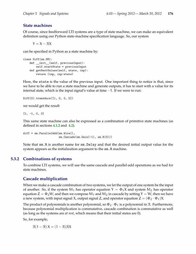
Chapter 5 Signals and Systems 6.01— Spring 2012—March 10, 2012 176
State machinesOf course, since feedforward LTI systems are a type of state machine, we can make an equivalentdefinition using our Python state-machine specification language. So, our system
Y = X− RX
can be specified in Python as a state machine by:
class Diff(sm.SM):def __init__(self, previousInput):
self.startState = previousInputdef getNextValues(self, state, inp):
return (inp, inp-state)
Here, the state is the value of the previous input. One important thing to notice is that, sincewe have to be able to run a state machine and generate outputs, it has to start with a value for itsinternal state, which is the input signal’s value at time −1. If we were to run:
Diff(0).transduce([1, 0, 0, 0])
we would get the result
[1, -1, 0, 0]
This same state machine can also be expressed as a combination of primitive state machines (asdefined in sections 4.1.2 and 4.2).
diff = sm.ParallelAdd(sm.Wire(),sm.Cascade(sm.Gain(-1), sm.R(0)))
Note that sm.R is another name for sm.Delay and that the desired initial output value for thesystem appears as the initialization argument to the sm.Rmachine.
5.3.2 Combinations of systemsTo combine LTI systems, we will use the same cascade and parallel-add operations as we had forstate machines.
Cascade multiplicationWhenwemake a cascade combination of two systems, we let the output of one system be the inputof another. So, if the system M1 has operator equation Y = Φ1X and system M2 has operatorequation Z = Φ2W, and then we composeM1 andM2 in cascade by setting Y =W, then we havea new system, with input signal X, output signal Z, and operator equation Z = (Φ2 ·Φ1)X.The product of polynomials is another polynomial, soΦ2 ·Φ1 is a polynomial in R. Furthermore,because polynomial multiplication is commutative, cascade combination is commutative as well(as long as the systems are at rest, which means that their initial states are 0).
So, for example,
R(1− R)X = (1− R)RX

Chapter 5 Signals and Systems 6.01— Spring 2012—March 10, 2012 177
and these two corresponding block diagrams are equivalent (the algebraic equivalence justifiesthe diagram equivalence):
Delay−1
+ DelayX Y
Delay−1
+DelayX Y
Cascade combination, because it results in multiplication, is also associative, which means thatany grouping of cascade operations on systems has the same result.
Exercise 5.5. Remembering that the condition on commutativity of cascading is that thesystems start at rest, explain why machines m3 and m4 do not generate thesame output sequence in response to the unit sample signal as input.
m1 = sm.ParallelAdd(sm.Wire(), sm.Cascade(sm.Gain(-1), sm.R(2)))m2 = sm.R(3)m3 = sm.Cascade(m1, m2)m4 = sm.Cascade(m2, m1)
Parallel additionWhen we make a parallel addition combination of two systems, the output signal is the sum ofthe output signals that would have resulted from the individual systems. So, if the systemM1 hassystem function Y = Φ1X and systemM2 has system function Z = Φ2X, and then we composeM1 andM2 with parallel addition by setting outputW = Y+Z, then we have a new system, withinput signal X, output signalW, and operator equationW = (Φ1 +Φ2)X.
Because addition of polynomials is associative and commutative, then so is parallel addition offeed-forward linear systems.
Combining cascade and parallel operationsFinally, the distributive law applies for cascade and parallel combination, for systems at rest, in thesame way that it applies for multiplication and addition of polynomials, so that if we have threesystems, with operator equations:
Y = Φ1X
U = Φ2V
W = Φ3Z ,
and we form a cascade combination of the sum of the first two, with the third, then we have asystem describable as:
B = (Φ3 · (Φ1 +Φ2))A .
We can rewrite this, using the distributive law, as:
B = ((Φ3 ·Φ1) + (Φ3 ·Φ2))A .
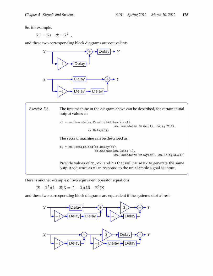
Chapter 5 Signals and Systems 6.01— Spring 2012—March 10, 2012 178
So, for example,
R(1− R) = R− R2 ,
and these two corresponding block diagrams are equivalent:
Delay−1
+ DelayX Y
−1
+
Delay Delay
DelayX Y
Exercise 5.6. The first machine in the diagram above can be described, for certain initialoutput values as:
m1 = sm.Cascade(sm.ParallelAdd(sm.Wire(),sm.Cascade(sm.Gain(-1), Delay(2))),
sm.Delay(3))
The second machine can be described as:
m2 = sm.ParallelAdd(sm.Delay(d1),sm.Cascade(sm.Gain(-1),
sm.Cascade(sm.Delay(d2), sm.Delay(d3))))
Provide values of d1, d2, and d3 that will cause m2 to generate the sameoutput sequence as m1 in response to the unit sample signal as input.
Here is another example of two equivalent operator equations
(R− R2)(2− R)X = (1− R)(2R− R2)X
and these two corresponding block diagrams are equivalent if the systems start at rest:
Delay
Delay Delay Delay−1
2
−1
+ +X Y
Delay
Delay
Delay Delay−1
2
−1
+ +X Y
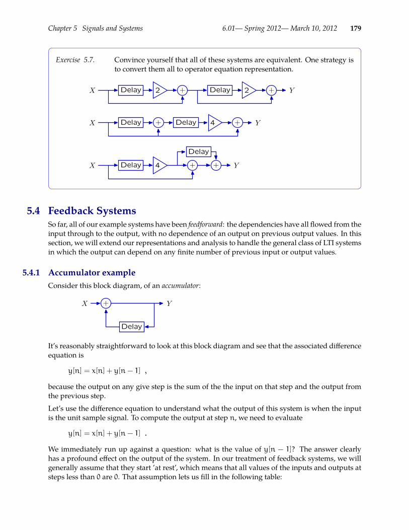
Chapter 5 Signals and Systems 6.01— Spring 2012—March 10, 2012 179
Exercise 5.7. Convince yourself that all of these systems are equivalent. One strategy isto convert them all to operator equation representation.
Delay 2 + Delay 2 +X Y
Delay + Delay 4 +X Y
Delay 4 +
Delay
+X Y
5.4 Feedback SystemsSo far, all of our example systems have been feedforward: the dependencies have all flowed from theinput through to the output, with no dependence of an output on previous output values. In thissection, we will extend our representations and analysis to handle the general class of LTI systemsin which the output can depend on any finite number of previous input or output values.
5.4.1 Accumulator exampleConsider this block diagram, of an accumulator:
Delay
+X Y
It’s reasonably straightforward to look at this block diagram and see that the associated differenceequation is
y[n] = x[n] + y[n− 1] ,
because the output on any give step is the sum of the the input on that step and the output fromthe previous step.
Let’s use the difference equation to understand what the output of this system is when the inputis the unit sample signal. To compute the output at step n, we need to evaluate
y[n] = x[n] + y[n− 1] .
We immediately run up against a question: what is the value of y[n − 1]? The answer clearlyhas a profound effect on the output of the system. In our treatment of feedback systems, we willgenerally assume that they start ’at rest’, which means that all values of the inputs and outputs atsteps less than 0 are 0. That assumption lets us fill in the following table:
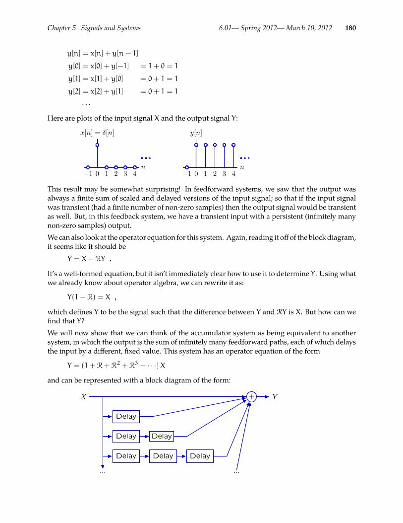
Chapter 5 Signals and Systems 6.01— Spring 2012—March 10, 2012 180
y[n] = x[n] + y[n− 1]
y[0] = x[0] + y[−1] = 1+ 0 = 1
y[1] = x[1] + y[0] = 0+ 1 = 1
y[2] = x[2] + y[1] = 0+ 1 = 1
· · ·
Here are plots of the input signal X and the output signal Y:
−1 0 1 2 3 4n
x[n] = δ[n]
−1 0 1 2 3 4n
y[n]
This result may be somewhat surprising! In feedforward systems, we saw that the output wasalways a finite sum of scaled and delayed versions of the input signal; so that if the input signalwas transient (had a finite number of non-zero samples) then the output signal would be transientas well. But, in this feedback system, we have a transient input with a persistent (infinitely manynon-zero samples) output.We can also look at the operator equation for this system. Again, reading it off of the block diagram,it seems like it should be
Y = X+ RY .
It’s a well-formed equation, but it isn’t immediately clear how to use it to determine Y. Using whatwe already know about operator algebra, we can rewrite it as:
Y(1− R) = X ,
which defines Y to be the signal such that the difference between Y and RY is X. But how can wefind that Y?We will now show that we can think of the accumulator system as being equivalent to anothersystem, in which the output is the sum of infinitely many feedforward paths, each of which delaysthe input by a different, fixed value. This system has an operator equation of the form
Y = (1+ R+ R2 + R3 + · · ·)X
and can be represented with a block diagram of the form:
Delay
Delay Delay
Delay Delay Delay
+
... ...
X Y
Chapter 5 Signals and Systems 6.01— Spring 2012—March 10, 2012 181
These systems are equivalent in the sense that if each is initially at rest, they will produce identicaloutputs from the same input. We can see this by taking the original definition and repeatedlysubstituting in the definition of Y in for its occurrence on the right hand side:
Y = X+ RY
Y = X+ R(X+ RY)
Y = X+ R(X+ R(X+ RY))
Y = X+ R(X+ R(X+ R(X+ RY)))
Y = (1+ R+ R2 + R3 + . . .)X
Now, we can informally derive a ’definition’ of the reciprocal of 1 − R (the mathematical detailsunderlying this are subtle and not presented here),
1
1− R= 1+ R+ R2 + R3 + · · · .
In the following it will help to remind ourselves of the derivation of the formula for the sum of aninfinte geometric series:
S = 1+ x+ x2 + x3 + · · ·
Sx = x+ x2 + x3 + x4 · · ·
Subtracting the second equation from the first we get
S(1− x) = 1
And so, provided |x| < 1,
1
1− x= 1+ x+ x2 + x3 + · · ·
Similarly, we can consider the system O, where
O = 1+ R+ R2 + R3 + · · ·
OR = R+ R2 + R3 + · · ·
So
O(1− R) = 1
And so,
1
1− R= 1+ R+ R2 + R3 + · · ·
Exercise 5.8. Check this derivation by showing that
(1+ R+ R2 + R3 + · · ·)(1− R) = 1
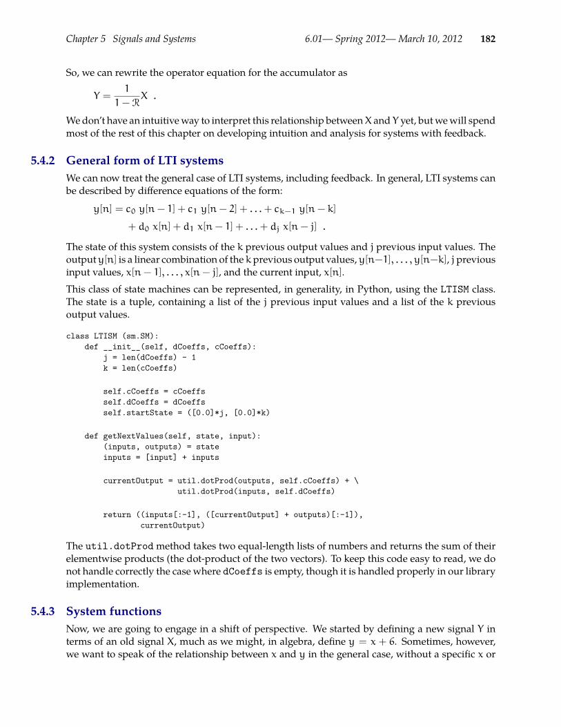
Chapter 5 Signals and Systems 6.01— Spring 2012—March 10, 2012 182
So, we can rewrite the operator equation for the accumulator as
Y =1
1− RX .
Wedon’t have an intuitiveway to interpret this relationship betweenX and Y yet, butwewill spendmost of the rest of this chapter on developing intuition and analysis for systems with feedback.
5.4.2 General form of LTI systemsWe can now treat the general case of LTI systems, including feedback. In general, LTI systems canbe described by difference equations of the form:
y[n] = c0 y[n− 1] + c1 y[n− 2] + . . .+ ck−1 y[n− k]
+ d0 x[n] + d1 x[n− 1] + . . .+ dj x[n− j] .
The state of this system consists of the k previous output values and j previous input values. Theoutputy[n] is a linear combination of the kprevious output values, y[n−1], . . . , y[n−k], jpreviousinput values, x[n− 1], . . . , x[n− j], and the current input, x[n].This class of state machines can be represented, in generality, in Python, using the LTISM class.The state is a tuple, containing a list of the j previous input values and a list of the k previousoutput values.
class LTISM (sm.SM):def __init__(self, dCoeffs, cCoeffs):
j = len(dCoeffs) - 1k = len(cCoeffs)
self.cCoeffs = cCoeffsself.dCoeffs = dCoeffsself.startState = ([0.0]*j, [0.0]*k)
def getNextValues(self, state, input):(inputs, outputs) = stateinputs = [input] + inputs
currentOutput = util.dotProd(outputs, self.cCoeffs) + \util.dotProd(inputs, self.dCoeffs)
return ((inputs[:-1], ([currentOutput] + outputs)[:-1]),currentOutput)
The util.dotProdmethod takes two equal-length lists of numbers and returns the sum of theirelementwise products (the dot-product of the two vectors). To keep this code easy to read, we donot handle correctly the case where dCoeffs is empty, though it is handled properly in our libraryimplementation.
5.4.3 System functionsNow, we are going to engage in a shift of perspective. We started by defining a new signal Y interms of an old signal X, much as we might, in algebra, define y = x + 6. Sometimes, however,we want to speak of the relationship between x and y in the general case, without a specific x or

Chapter 5 Signals and Systems 6.01— Spring 2012—March 10, 2012 183
y in mind. We do this by defining a function f: f(x) = x + 6. We can do the same thing with LTIsystems, by defining system functions.
If we take the general formof an LTI systemgiven in the previous section andwrite it as an operatorequation, we have
Y = c0 RY + c1 R2Y + . . .+ ck−1 R
kY + d0 X+ d1 RX+ . . .+ dj RjX
= (c0 R+ c1 R2 + . . .+ ck−1 R
k) Y + (d0 + d1 R+ . . .+ dj Rj) X .
We can rewrite this as
(1− c0 R− c1 R2 − . . .− ck−1 R
k) Y = (d0 + d1 R+ . . .+ dj Rj) X ,
soY
X=d0 + d1R+ d2R
2 + d3R3 + · · ·
1− c0R− c1R2 − c2R3 − · · ·,
which has the formY
X=N(R)
D(R),
where N(R), the numerator, is a polynomial in R, and D(R), the denominator, is also a polyno-mial in R. We will refer to Y/X as the system function: it characterizes the operation of a system,independent of the particular input and output signals involved.
The system function is most typically written in the form
Y
X=b0 + b1R+ b2R
2 + b3R3 + · · ·
a0 + a1R+ a2R2 + a3R3 + · · ·,
where ci = −ai+1/a0 and di = bi/a0. It can be completely characterized by the coefficients ofthe denominator polynomial, ai, and the coefficients of the numerator polynomial, bi. It is alwayspossible to rewrite this in a form in which a0 = 1.
Feedforward systems have no dependence on previous values of Y, so they haveD(R) = 1. Feed-back systems have persistent behavior, which is determined by D(R). We will study this depen-dence in detail in section 5.5.
5.4.4 Primitive systemsJust aswe had a PCAP system for signals, we have one for LTI system, in terms of system functions,as well. We can specify system functions for each of our system primitives.
A gain element is governed by operator equation Y = kX, for constant k, so its system function is
H =Y
X= k .
A delay element is governed by operator equation Y = RX, so its system function is
H =Y
X= R .
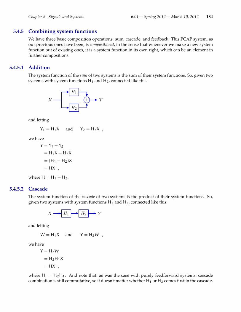
Chapter 5 Signals and Systems 6.01— Spring 2012—March 10, 2012 184
5.4.5 Combining system functionsWe have three basic composition operations: sum, cascade, and feedback. This PCAP system, asour previous ones have been, is compositional, in the sense that whenever we make a new systemfunction out of existing ones, it is a system function in its own right, which can be an element infurther compositions.
5.4.5.1 AdditionThe system function of the sum of two systems is the sum of their system functions. So, given twosystems with system functions H1 and H2, connected like this:
H1
H2
+X Y
and letting
Y1 = H1X and Y2 = H2X ,
we haveY = Y1 + Y2
= H1X+H2X
= (H1 +H2)X
= HX ,
where H = H1 +H2.
5.4.5.2 CascadeThe system function of the cascade of two systems is the product of their system functions. So,given two systems with system functions H1 and H2, connected like this:
H1 H2X Y
and letting
W = H1X and Y = H2W ,
we haveY = H2W
= H2H1X
= HX ,
where H = H2H1. And note that, as was the case with purely feedforward systems, cascadecombination is still commutative, so it doesn’t matter whetherH1 orH2 comes first in the cascade.

Chapter 5 Signals and Systems 6.01— Spring 2012—March 10, 2012 185
This surprising fact holds because we are only considering LTI systems starting at rest; for moregeneral classes of systems, such as the general class of state machines we have workedwith before,the ordering of a cascade does matter.
5.4.5.3 FeedbackThere are several ways of connecting systems in feedback. Here we study a particular case ofnegative feedback combination, which results in a classical formula called Black’s formula.
Consider two systems connected like this
H1
H2
+X Y−
and pay careful attention to the negative sign on the feedback input to the addition. It is really just short-hand; the negative sign could be replaced with a gain component with value −1. This negativefeedback arrangement is frequently used to model a case in which X is a desired value for somesignal and Y is its actual value; thus the input toH1 is the difference between the desired an actualvalues, often called an error signal. We can simply write down the operator equation governingthis system and use standard algebraic operations to determine the system function:
Y = H1(X−H2Y)
Y +H1H2Y = H1X
Y(1+H1H2) = H1X
Y =H1
1+H1H2X
Y = HX ,
where
H =H1
1+H1H2.
Armed with this set of primitives and composition methods, we can specify a large class of ma-chines. Ultimately, we will want to construct systems with multiple inputs and outputs; such sys-tems are specified with a matrix of basic system functions, describing how each output dependson each input.
5.5 Predicting system behaviorWe have seen how to construct complex discrete-time LTI systems; in this section we will see howwe can use properties of the system function to predict how the system will behave, in the longterm, and for any input. Wewill start by analyzing simple systems and thenmove tomore complexones.
We can provide a general characterization of the long-term behavior of the output, as increasing ordecreasing, with constant or alternating sign, for any finite input to the system. We will begin by
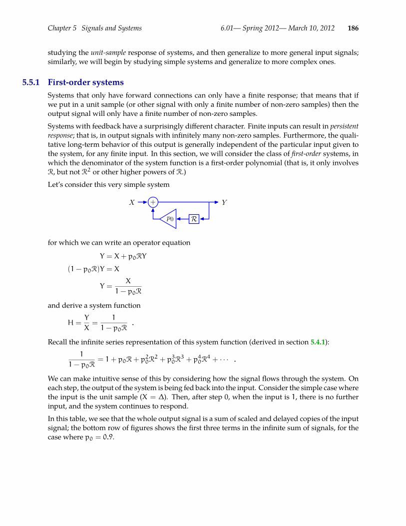
Chapter 5 Signals and Systems 6.01— Spring 2012—March 10, 2012 186
studying the unit-sample response of systems, and then generalize to more general input signals;similarly, we will begin by studying simple systems and generalize to more complex ones.
5.5.1 First-order systemsSystems that only have forward connections can only have a finite response; that means that ifwe put in a unit sample (or other signal with only a finite number of non-zero samples) then theoutput signal will only have a finite number of non-zero samples.
Systems with feedback have a surprisingly different character. Finite inputs can result in persistentresponse; that is, in output signals with infinitely many non-zero samples. Furthermore, the quali-tative long-term behavior of this output is generally independent of the particular input given tothe system, for any finite input. In this section, we will consider the class of first-order systems, inwhich the denominator of the system function is a first-order polynomial (that is, it only involvesR, but not R2 or other higher powers of R.)
Let’s consider this very simple system
+
Rp0
X Y
for which we can write an operator equation
Y = X+ p0RY
(1− p0R)Y = X
Y =X
1− p0R
and derive a system function
H =Y
X=
1
1− p0R.
Recall the infinite series representation of this system function (derived in section 5.4.1):1
1− p0R= 1+ p0R+ p20R
2 + p30R3 + p40R
4 + · · · .
We can make intuitive sense of this by considering how the signal flows through the system. Oneach step, the output of the system is being fed back into the input. Consider the simple casewherethe input is the unit sample (X = ∆). Then, after step 0, when the input is 1, there is no furtherinput, and the system continues to respond.
In this table, we see that the whole output signal is a sum of scaled and delayed copies of the inputsignal; the bottom row of figures shows the first three terms in the infinite sum of signals, for thecase where p0 = 0.9.
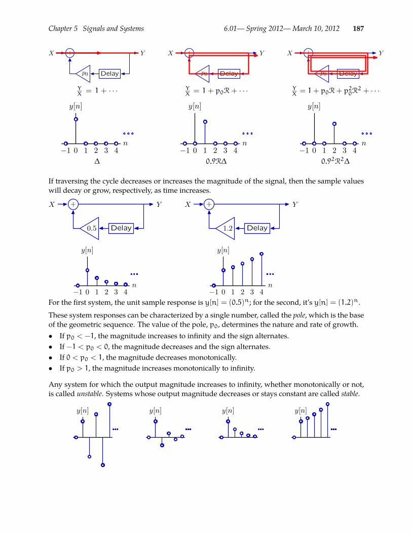
Chapter 5 Signals and Systems 6.01— Spring 2012—March 10, 2012 187
Delay
+
p0
X Y
Delay
+
p0
X Y
Delay
+
p0
X Y
YX = 1 + · · · Y
X = 1 + p0R + · · · YX = 1 + p0R + p20R
2 + · · ·
−1 0 1 2 3 4n
y[n]
−1 0 1 2 3 4n
y[n]
−1 0 1 2 3 4n
y[n]
∆ 0.9R∆ 0.92R2∆
If traversing the cycle decreases or increases the magnitude of the signal, then the sample valueswill decay or grow, respectively, as time increases.
Delay
+
0.5
X Y
Delay
+
1.2
X Y
−1 0 1 2 3 4n
y[n]
−1 0 1 2 3 4n
y[n]
For the first system, the unit sample response is y[n] = (0.5)n; for the second, it’s y[n] = (1.2)n.
These system responses can be characterized by a single number, called the pole, which is the baseof the geometric sequence. The value of the pole, p0, determines the nature and rate of growth.• If p0 < −1, the magnitude increases to infinity and the sign alternates.• If −1 < p0 < 0, the magnitude decreases and the sign alternates.• If 0 < p0 < 1, the magnitude decreases monotonically.• If p0 > 1, the magnitude increases monotonically to infinity.
Any system for which the output magnitude increases to infinity, whether monotonically or not,is called unstable. Systems whose output magnitude decreases or stays constant are called stable.
y[n] y[n] y[n] y[n]

Chapter 5 Signals and Systems 6.01— Spring 2012—March 10, 2012 188
−1 0 1z
5.5.2 Second-order systemsWe will call these persistent long-term behaviors of a signal (and, hence, of the system that gen-erates such signals) modes. For a fixed p0, the first-order system only exhibited one mode (butdifferent values of p0 resulted in very different modes). As we build more complex systems, theywill have multiple modes, which manifest as more complex behavior. Second-order systems arecharacterized by a system function whose denominator polynomial is second order; they will gen-erally exhibit two modes. We will find that it is the mode whose pole has the largest magnitudethat governs the long-term behavior of the system. We will call this pole the dominant pole.
Consider this system
R
R
1.6
−0.63
+X Y
We can describe it with the operator equation
Y = 1.6RY − 0.63R2Y + X ,
so the system function is
H =1
1− 1.6R+ 0.63R2.
Here is its response to a unit sample signal:
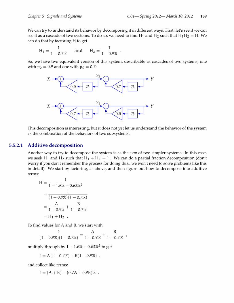
Chapter 5 Signals and Systems 6.01— Spring 2012—March 10, 2012 189
We can try to understand its behavior by decomposing it in different ways. First, let’s see if we cansee it as a cascade of two systems. To do so, we need to find H1 and H2 such that H1H2 = H. Wecan do that by factoring H to get
H1 =1
1− 0.7Rand H2 =
1
1− 0.9R.
So, we have two equivalent version of this system, describable as cascades of two systems, onewith p0 = 0.9 and one with p0 = 0.7:
+
0.9 R
+
0.7 R
X YY2
+
0.7 R
+
0.9 R
X YY1
This decomposition is interesting, but it does not yet let us understand the behavior of the systemas the combination of the behaviors of two subsystems.
5.5.2.1 Additive decompositionAnother way to try to decompose the system is as the sum of two simpler systems. In this case,we seek H1 and H2 such that H1 + H2 = H. We can do a partial fraction decomposition (don’tworry if you don’t remember the process for doing this...we won’t need to solve problems like thisin detail). We start by factoring, as above, and then figure out how to decompose into additiveterms:
H =1
1− 1.6R+ 0.63R2
=1
(1− 0.9R)(1− 0.7R)
=A
1− 0.9R+
B
1− 0.7R
= H1 +H2 .
To find values for A and B, we start with1
(1− 0.9R)(1− 0.7R)=
A
1− 0.9R+
B
1− 0.7R,
multiply through by 1− 1.6R+ 0.63R2 to get
1 = A(1− 0.7R) + B(1− 0.9R) ,
and collect like terms:
1 = (A+ B) − (0.7A+ 0.9B)R .
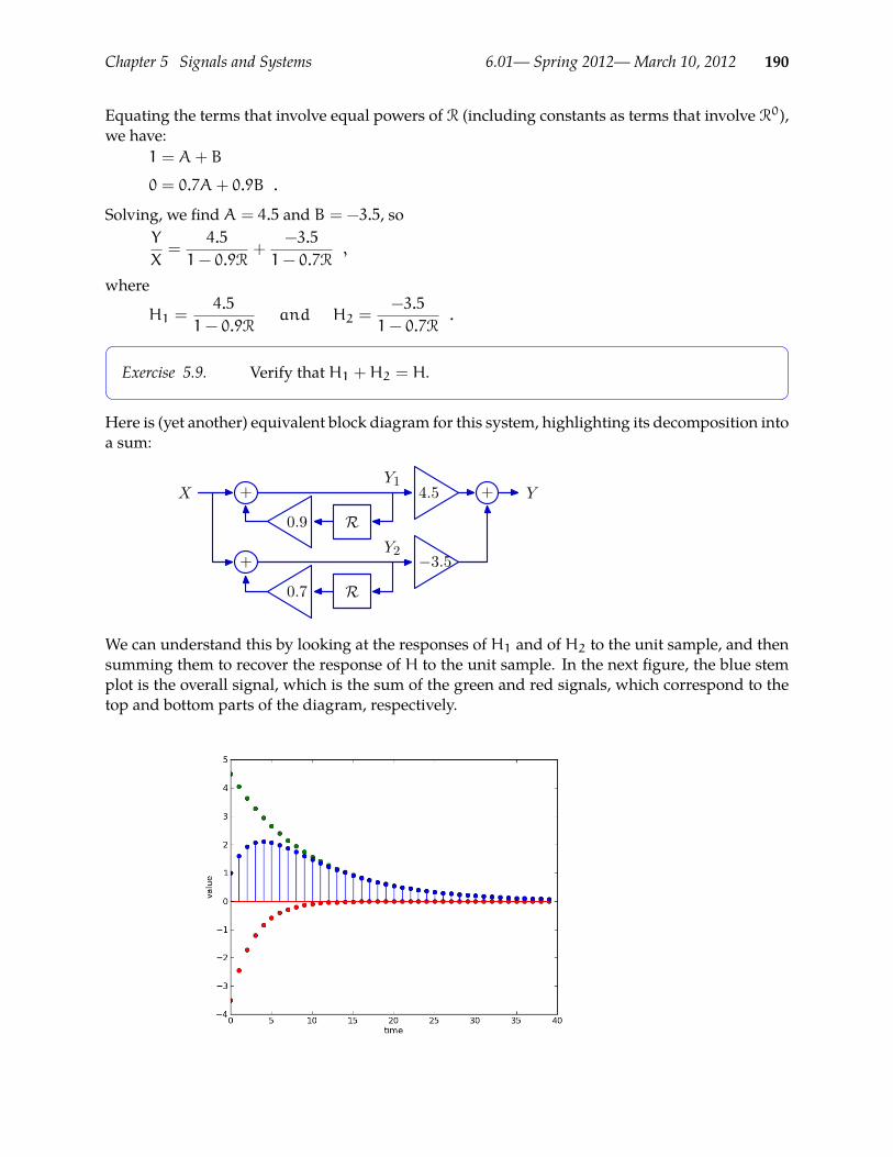
Chapter 5 Signals and Systems 6.01— Spring 2012—March 10, 2012 190
Equating the terms that involve equal powers of R (including constants as terms that involve R0),we have:
1 = A+ B
0 = 0.7A+ 0.9B .
Solving, we find A = 4.5 and B = −3.5, soY
X=
4.5
1− 0.9R+
−3.5
1− 0.7R,
where
H1 =4.5
1− 0.9Rand H2 =
−3.5
1− 0.7R.
Exercise 5.9. Verify that H1 +H2 = H.
Here is (yet another) equivalent block diagram for this system, highlighting its decomposition intoa sum:
+
0.9 R
4.5 +
−3.5
R0.7
+
X YY1
Y2
We can understand this by looking at the responses of H1 and of H2 to the unit sample, and thensumming them to recover the response of H to the unit sample. In the next figure, the blue stemplot is the overall signal, which is the sum of the green and red signals, which correspond to thetop and bottom parts of the diagram, respectively.
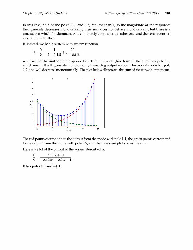
Chapter 5 Signals and Systems 6.01— Spring 2012—March 10, 2012 191
In this case, both of the poles (0.9 and 0.7) are less than 1, so the magnitude of the responsesthey generate decreases monotonically; their sum does not behave monotonically, but there is atime step at which the dominant pole completely dominates the other one, and the convergence ismonotonic after that.
If, instead, we had a system with system function
H =Y
X=
1
1− 1.1R+
20
1− 0.9R,
what would the unit-sample response be? The first mode (first term of the sum) has pole 1.1,which means it will generate monotonically increasing output values. The second mode has pole0.9, and will decrease monotonically. The plot below illustrates the sum of these two components:
The red points correspond to the output from themodewith pole 1.1; the green points correspondto the output from the mode with pole 0.9; and the blue stem plot shows the sum.
Here is a plot of the output of the system described byY
X=
21.1R+ 21
−0.99R2 + 0.2R+ 1.
It has poles 0.9 and −1.1.
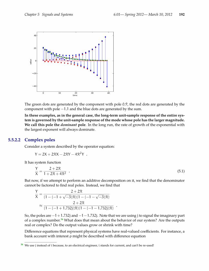
Chapter 5 Signals and Systems 6.01— Spring 2012—March 10, 2012 192
The green dots are generated by the component with pole 0.9, the red dots are generated by thecomponent with pole −1.1 and the blue dots are generated by the sum.
In these examples, as in the general case, the long-term unit-sample response of the entire sys-tem is governed by the unit-sample response of themodewhose pole has the larger magnitude.We call this pole the dominant pole. In the long run, the rate of growth of the exponential withthe largest exponent will always dominate.
5.5.2.2 Complex polesConsider a system described by the operator equation:
Y = 2X+ 2RX− 2RY − 4R2Y .
It has system functionY
X=
2+ 2R
1+ 2R+ 4R2. (5.1)
But now, if we attempt to perform an additive decomposition on it, we find that the denominatorcannot be factored to find real poles. Instead, we find that
Y
X=
2+ 2R
(1− (−1+√−3)R)(1− (−1−
√−3)R)
≈ 2+ 2R
(1− (−1+ 1.732j)R)(1− (−1− 1.732j)R).
So, the poles are−1+1.732j and−1−1.732j. Note that we are using j to signal the imaginary partof a complex number.36 What does that mean about the behavior of our system? Are the outputsreal or complex? Do the output values grow or shrink with time?
Difference equations that represent physical systems have real-valued coefficients. For instance, abank account with interest ρmight be described with difference equation
We use j instead of i because, to an electrical engineer, i stands for current, and can’t be re-used!36
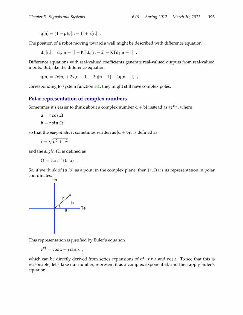
Chapter 5 Signals and Systems 6.01— Spring 2012—March 10, 2012 193
y[n] = (1+ ρ)y[n− 1] + x[n] .
The position of a robot moving toward a wall might be described with difference equation:
do[n] = do[n− 1] + KTdo[n− 2] − KTdi[n− 1] .
Difference equations with real-valued coefficients generate real-valued outputs from real-valuedinputs. But, like the difference equation
y[n] = 2x[n] + 2x[n− 1] − 2y[n− 1] − 4y[n− 1] ,
corresponding to system function 5.1, they might still have complex poles.
Polar representation of complex numbersSometimes it’s easier to think about a complex number a+ bj instead as rejΩ, where
a = r cosΩ
b = r sinΩ
so that the magnitude, r, sometimes written as |a+ bj|, is defined as
r =√a2 + b2
and the angle,Ω, is defined as
Ω = tan−1(b, a) .
So, if we think of (a, b) as a point in the complex plane, then (r,Ω) is its representation in polarcoordinates.
ab
r
Ω Re
Im
This representation is justified by Euler’s equation
exj = cos x+ j sin x ,
which can be directly derived from series expansions of ez, sin z and cos z. To see that this isreasonable, let’s take our number, represent it as a complex exponential, and then apply Euler’sequation:

Chapter 5 Signals and Systems 6.01— Spring 2012—March 10, 2012 194
a+ bj = rejΩ
= r(cosΩ+ j sinΩ)
=√a2 + b2(cos(tan−1(b, a)) + j sin(tan−1(b, a)))
=√a2 + b2(
a√a2 + b2
+ jb√
a2 + b2)
= a+ bj
Why should we bother with this change of representation? There are some operations on complexnumbers that are much more straightforwardly done in the exponential representation. In partic-ular, let’s consider raising a complex number to a power. In the Cartesian representation, we getcomplex trigonometric polynomials. In the exponential representation, we get, in the quadraticcase, (
rejΩ)2
= rejΩrejΩ
= r2ej2Ω
More generally, we have that(rejΩ
)n= rnejnΩ ,
which is much tidier. This is an instance of an important trick in math and engineering: changingrepresentations. We will often find that representing something in a different way will allow usto do some kinds of manipulations more easily. This is why we use diagrams, difference equa-tions, operator equations and system functions all to describe LTI systems. There is no one bestrepresentation; each has advantages under some circumstances (and disadvantages under others).
Complex modesNow, we’re equipped to understand how complex poles of a system generate behavior: they pro-duce complex-valued modes. Remember that we can characterize the behavior of a mode as
1
1− pR= 1+ pR+ p2R2 + · · ·+ pnRn + · · · .
For a complex pole p = rejΩ, pn = rnejΩn. So1
1− rejΩR= 1+ rejΩR+ r2ej2ΩR2 + · · ·
What happens as n tends to infinity when p is complex? Think of pn as a point in the complexplane with coordinates (rn,Ωn). The radius, rn, will grow or shrink depending on the mode’smagnitude, r. And the angle, Ωn, will simply rotate, but will not affect the magnitude of theresulting value. Note that each new point in the sequence pn will be rotated by Ω from the pre-vious one. We will say that the period of the output signal is 2π/Ω; that is the number of samplesrequired to move through 2π radians (although this need not actually be an integer).
The sequence spirals around the origin of the complex plane. Here is a case for r = 0.85,Ω = π/4,that spirals inward, rotating π/4 radians on each step:
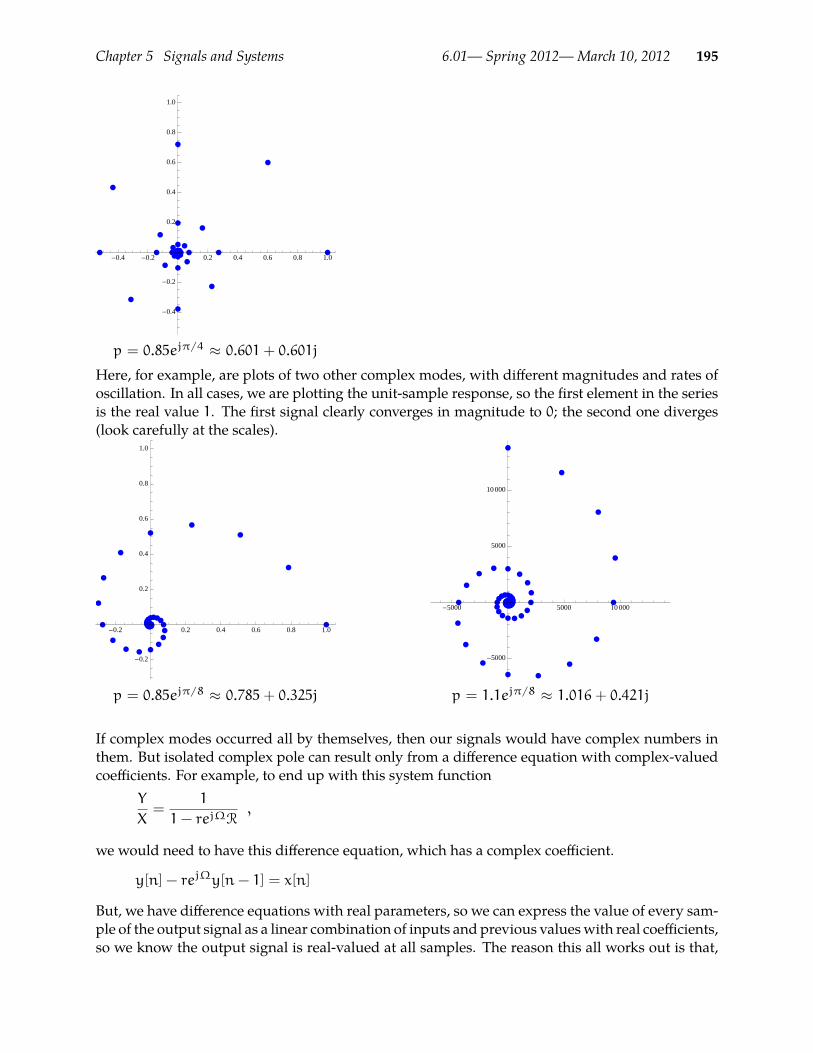
Chapter 5 Signals and Systems 6.01— Spring 2012—March 10, 2012 195
-0.4 -0.2 0.2 0.4 0.6 0.8 1.0
-0.4
-0.2
0.2
0.4
0.6
0.8
1.0
p = 0.85ejπ/4 ≈ 0.601 + 0.601jHere, for example, are plots of two other complex modes, with different magnitudes and rates ofoscillation. In all cases, we are plotting the unit-sample response, so the first element in the seriesis the real value 1. The first signal clearly converges in magnitude to 0; the second one diverges(look carefully at the scales).
-0.2 0.2 0.4 0.6 0.8 1.0
-0.2
0.2
0.4
0.6
0.8
1.0
-5000 5000 10 000
-5000
5000
10 000
p = 0.85ejπ/8 ≈ 0.785 + 0.325j p = 1.1ejπ/8 ≈ 1.016 + 0.421j
If complex modes occurred all by themselves, then our signals would have complex numbers inthem. But isolated complex pole can result only from a difference equation with complex-valuedcoefficients. For example, to end up with this system function
Y
X=
1
1− rejΩR,
we would need to have this difference equation, which has a complex coefficient.
y[n] − rejΩy[n− 1] = x[n]
But, we have difference equations with real parameters, so we can express the value of every sam-ple of the output signal as a linear combination of inputs and previous valueswith real coefficients,so we know the output signal is real-valued at all samples. The reason this all works out is that,
Chapter 5 Signals and Systems 6.01— Spring 2012—March 10, 2012 196
for polynomials with real coefficients, the complex poles always come in conjugate pairs: that is,pairs of complex numbers p = a + bj and p∗ = a − bj. (See section 5.5.4 for a proof of this fact.)In the polar representation, the conjugate pair becomes
a± bj =√a2 + b2 ej tan
−1(±b,a)
=√a2 + b2 e±j tan
−1(b,a)
where the only difference is in the sign of the angular part.
If we look at a second-order system with complex-conjugate poles, the resulting polynomial hasreal-valued coefficients. To see this, consider a system with poles rejΩ and re−jΩ, so that
Y
X=
1
(1− rejΩR)(1− re−jΩR)
Let’s slowly multiply out the denominator:
(1− rejΩR)(1− re−jΩR) = 1− rejΩR− re−jΩR+ r2ejΩe−jΩR2
= 1− r(ejΩ + e−jΩ)R+ r2ejΩ−jΩR2
Using the definition of the complex exponential ejx = cos x+ j sin x,
= 1− r(cosΩ+ j sinΩ+ cos(−Ω) + j sin(−Ω))R+ r2R2
Using trigonometric identities sin−x = − sin x and cos−x = cos x,
= 1− r(cosΩ+ j sinΩ+ cosΩ− j sinΩ)R+ r2R2
= 1− 2r cosΩR+ r2R2
So,Y
X=
1
1− 2r cosΩR+ r2R2.
This is pretty cool! All of the imaginary parts cancel, and we are left with a system function withonly real coefficients, which corresponds to the difference equation
y[n] = x[n] + 2r cosΩ y[n− 1] − r2y[n− 2] .
Additive decomposition with complex polesYou can skip this section if you want to.To really understand these complex modes and how they combine to generate the outputsignal, we need to do an additive decomposition. That means doing a partial fraction ex-pansion of
Y
X=
1
(1− rejΩR)(1− re−jΩR).
It’s a little trickier than before, because we have complex numbers, but the method is the same.The end result is that we can decompose this system additively to get
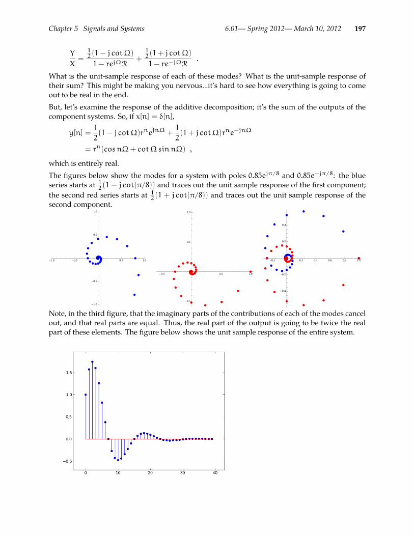
Chapter 5 Signals and Systems 6.01— Spring 2012—March 10, 2012 197
Y
X=12(1− j cotΩ)
1− rejΩR+12(1+ j cotΩ)
1− re−jΩR.
What is the unit-sample response of each of these modes? What is the unit-sample response oftheir sum? This might be making you nervous...it’s hard to see how everything is going to comeout to be real in the end.But, let’s examine the response of the additive decomposition; it’s the sum of the outputs of thecomponent systems. So, if x[n] = δ[n],
y[n] =1
2(1− j cotΩ)rnejnΩ +
1
2(1+ j cotΩ)rne−jnΩ
= rn(cosnΩ+ cotΩsinnΩ) ,
which is entirely real.The figures below show the modes for a system with poles 0.85ejπ/8 and 0.85e−jπ/8: the blueseries starts at 12(1 − j cot(π/8)) and traces out the unit sample response of the first component;the second red series starts at 12(1 + j cot(π/8)) and traces out the unit sample response of thesecond component.
-1.0 -0.5 0.5 1.0
-1.0
-0.5
0.5
1.0
-0.5 0.5 1.0
-0.5
0.5
1.0
-0.2 0.2 0.4 0.6 0.8 1.0
-0.4
-0.2
0.2
0.4
Note, in the third figure, that the imaginary parts of the contributions of each of the modes cancelout, and that real parts are equal. Thus, the real part of the output is going to be twice the realpart of these elements. The figure below shows the unit sample response of the entire system.

Chapter 5 Signals and Systems 6.01— Spring 2012—March 10, 2012 198
In the formula below,
y[n] = rn(cosnΩ+ cotΩsinnΩ) ,
we know that
−√1+ cot2Ω 6 cosnΩ+ cotΩsinnΩ 6
√1+ cot2Ω ,
so
−√1+ cot2Ω rn 6 y[n] 6
√1+ cot2Ω rn
−1
sinΩrn 6 y[n] 6
1
sinΩrn .
Just for fun, here is a three-dimensional plot of a single mode of a system with pole 0.98ejπ/20.These valueswere chosen so that it would shrink slowly and also rotate slowly around the complexplane. The first figure showsn growing upwardwith the complex plane oriented horizontally; thesecond shows a view looking down onto the complex plane; the third shows a view that projectsalong the imaginary axis.
-10
12
re
-2
0
2
im
0
50
100
n
-1 0 1 2
re
-2
0
2
im
050100n
-1012
re
-202 im
0
50
100
n
Importance of magnitude and periodBoth r and Ω tells us something very useful about the way in which the system behaves. In theprevious section, wederived an expression for the samples of the unit sample response for a systemwith a pair of complex poles. It has the form
y[n] = rn(cosnΩ+ αsinnΩ) ,
where α is a constant. We know that (cosnΩ+αsinnΩ) cannot possibly be less than−√1+ α2
or greater than√1+ α2.

Chapter 5 Signals and Systems 6.01— Spring 2012—March 10, 2012 199
These bounds provide an envelope that constrainswhere the values of the signal can be as a functionof time, and help us understand the rate of growth or decay of the signal, as shown below. Thered and green curves are ±
√1+ α2rn, for a system where r = 0.85,Ω = π/8, and α = 2.414.
The value of r governs the rate of exponential decrease. The value ofΩ governs the rate of oscilla-tion of the curve. It will take 2π/Ω (the period of the oscillation) samples to go from peak to peakof the oscillation.37 In our example, Ω = π/8 so the period is 16; you should be able to count 16samples from peak to peak.
5.5.2.3 Poles and behavior: summaryIn a second-order system, if we let p0 be the pole with the largest magnitude, then there is a timestep at which the behavior of the dominant pole begins to dominate; after that time step• If p0 is real and• p0 < −1, the magnitude increases to infinity and the sign alternates.• −1 < p0 < 0, the magnitude decreases and the sign alternates.• 0 < p0 < 1, the magnitude decreases monotonically.• p0 > 1, the magnitude increases monotonically to infinity.
• If p0 is complex• and |p0| < 1, the magnitude decreases monotonically.• and |p0| > 1, the magnitude increases monotonically to infinity.
• If p0 is complex andΩ is its angle, then the signal will be periodic, with period 2π/Ω.Remember that any system for which the output magnitude increases to infinity, whether monot-onically or not, is called unstable. Systems whose output magnitude decreases or stays constantare called stable.As we have seen in our examples, when we add multiple modes, it is the mode with the largestpole, that is, the dominant pole that governs the long-term behavior.
We are being informal here, in two ways. First, the signal does not technically have a period, because unless r = 1, it37
doesn’t return to the same point. Second, unless r = 1, then distance from peak to peak is not exactly 2π/Ω, however,for most signals, it will give a good basis for estimatingΩ.
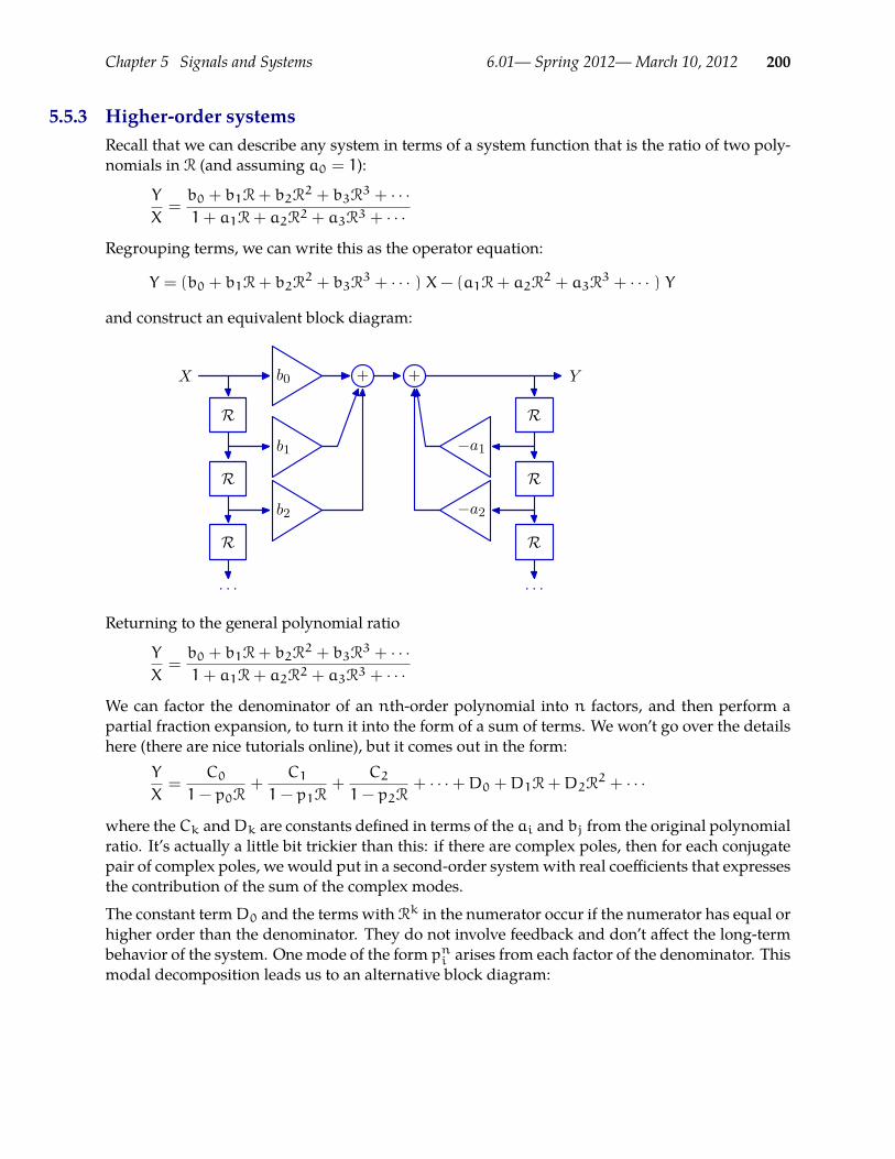
Chapter 5 Signals and Systems 6.01— Spring 2012—March 10, 2012 200
5.5.3 Higher-order systemsRecall that we can describe any system in terms of a system function that is the ratio of two poly-nomials in R (and assuming a0 = 1):
Y
X=b0 + b1R+ b2R
2 + b3R3 + · · ·
1+ a1R+ a2R2 + a3R3 + · · ·
Regrouping terms, we can write this as the operator equation:
Y = (b0 + b1R+ b2R2 + b3R
3 + · · · ) X− (a1R+ a2R2 + a3R
3 + · · · ) Y
and construct an equivalent block diagram:
R
R
R
R
R
R
−a1
−a2
b0
b1
b2
+ +
· · · · · ·
X Y
Returning to the general polynomial ratio
Y
X=b0 + b1R+ b2R
2 + b3R3 + · · ·
1+ a1R+ a2R2 + a3R3 + · · ·
We can factor the denominator of an nth-order polynomial into n factors, and then perform apartial fraction expansion, to turn it into the form of a sum of terms. We won’t go over the detailshere (there are nice tutorials online), but it comes out in the form:
Y
X=
C0
1− p0R+
C1
1− p1R+
C2
1− p2R+ · · ·+D0 +D1R+D2R
2 + · · ·
where theCk andDk are constants defined in terms of the ai and bj from the original polynomialratio. It’s actually a little bit trickier than this: if there are complex poles, then for each conjugatepair of complex poles, we would put in a second-order systemwith real coefficients that expressesthe contribution of the sum of the complex modes.
The constant termD0 and the terms withRk in the numerator occur if the numerator has equal orhigher order than the denominator. They do not involve feedback and don’t affect the long-termbehavior of the system. One mode of the form pni arises from each factor of the denominator. Thismodal decomposition leads us to an alternative block diagram:
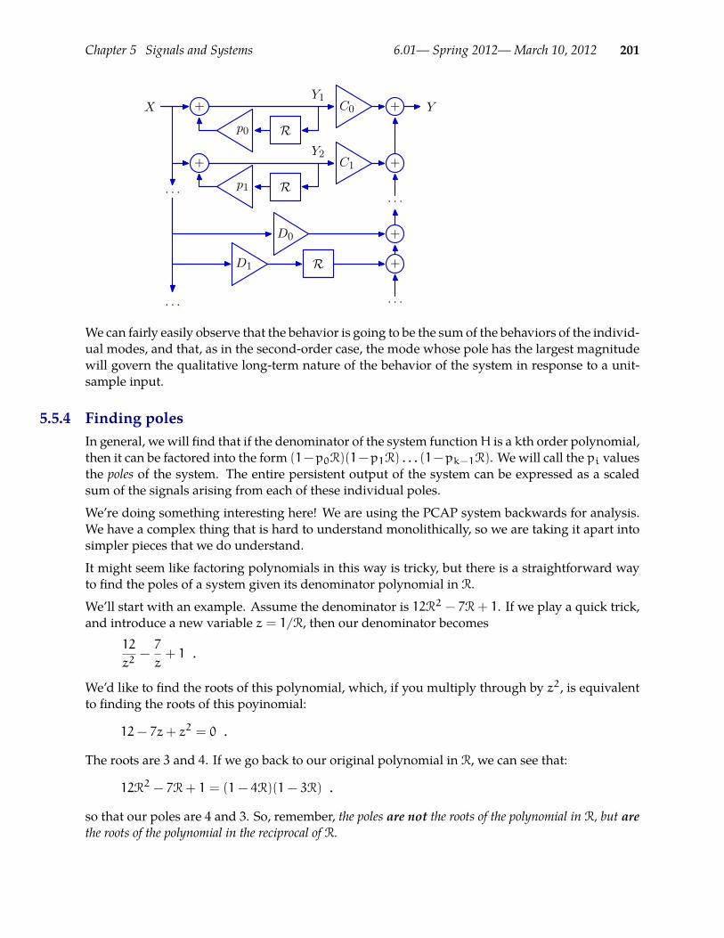
Chapter 5 Signals and Systems 6.01— Spring 2012—March 10, 2012 201
+p0 R
C0 +
C1
Rp1
+ +
D0
D1 R
+
+
· · ·· · ·
· · · · · ·
X YY1
Y2
We can fairly easily observe that the behavior is going to be the sum of the behaviors of the individ-ual modes, and that, as in the second-order case, the mode whose pole has the largest magnitudewill govern the qualitative long-term nature of the behavior of the system in response to a unit-sample input.
5.5.4 Finding polesIn general, we will find that if the denominator of the system functionH is a kth order polynomial,then it can be factored into the form (1−p0R)(1−p1R) . . . (1−pk−1R). We will call the pi valuesthe poles of the system. The entire persistent output of the system can be expressed as a scaledsum of the signals arising from each of these individual poles.
We’re doing something interesting here! We are using the PCAP system backwards for analysis.We have a complex thing that is hard to understand monolithically, so we are taking it apart intosimpler pieces that we do understand.
It might seem like factoring polynomials in this way is tricky, but there is a straightforward wayto find the poles of a system given its denominator polynomial in R.
We’ll start with an example. Assume the denominator is 12R2 − 7R + 1. If we play a quick trick,and introduce a new variable z = 1/R, then our denominator becomes
12
z2−7
z+ 1 .
We’d like to find the roots of this polynomial, which, if you multiply through by z2, is equivalentto finding the roots of this poyinomial:
12− 7z+ z2 = 0 .
The roots are 3 and 4. If we go back to our original polynomial in R, we can see that:
12R2 − 7R+ 1 = (1− 4R)(1− 3R) .
so that our poles are 4 and 3. So, remember, the poles are not the roots of the polynomial in R, but arethe roots of the polynomial in the reciprocal of R.

Chapter 5 Signals and Systems 6.01— Spring 2012—March 10, 2012 202
The roots of a polynomial can be a combination of real and complex numbers, with the requirementthat if a complex number p is a root, then so is its complex conjugate, p∗.
Pole-Zero cancellationFor some systems, we may find that it is possible to cancel matching factors from the numeratorand denominator of the system function. If the factors represent poles that are not at zero, thenalthough it may be theoretically supportable to cancel them, it is unlikely that they would matchexactly in a real system. If we were to cancel them in that case, we might end up with a systemmodel that was a particularly poor match for reality.38
So, we will only consider canceling poles and zeros at zero. In this example:
H =R
R− 1.6R2 + 0.63R3
we can cancel R, getting
H =1
1− 1.6R+ 0.63R2
Now, we find the poles by finding the roots of the equation
z2 − 1.6z+ 0.63 = 0
Repeated rootsIn some cases, the equation in zwill have repeated roots. For example, z2−z+0.25, which has tworoots at 0.5. In this case, the system has a repeated pole; it is still possible to perform an additivedecomposition, but it is somewhat trickier. Ultimately, however, it is still the magnitude of thelargest root that governs the long-term convergence properties of the system.
5.5.5 SuperpositionThe principle of superposition states that the response of a LTI system to a sum of input signals isthe sum of the responses of that system to the components of the input. So, given a system withsystem function H, and input X = X1 + X2,
Y = HX = H(X1 + X2) = HX1 +HX2
So, although we have been concentrating on the unit sample response of systems, we can see that,to find the response of a system to any finite signal, we must simply sum the responses to eachof the components of that signal; and those responses will simply be scaled, delayed copies of theresponse to the unit sample.
If Φ is a polynomial in R and X = Φ∆, then we can use what we know about the algebra ofpolynomials in R (remembering that H is a ratio of polynomials in R) to determine that
Y = HX = H(Φ∆) = Φ(H∆)
Don’t worry too much if this doesn’t make sense to you...take 6.003 to learn more.38
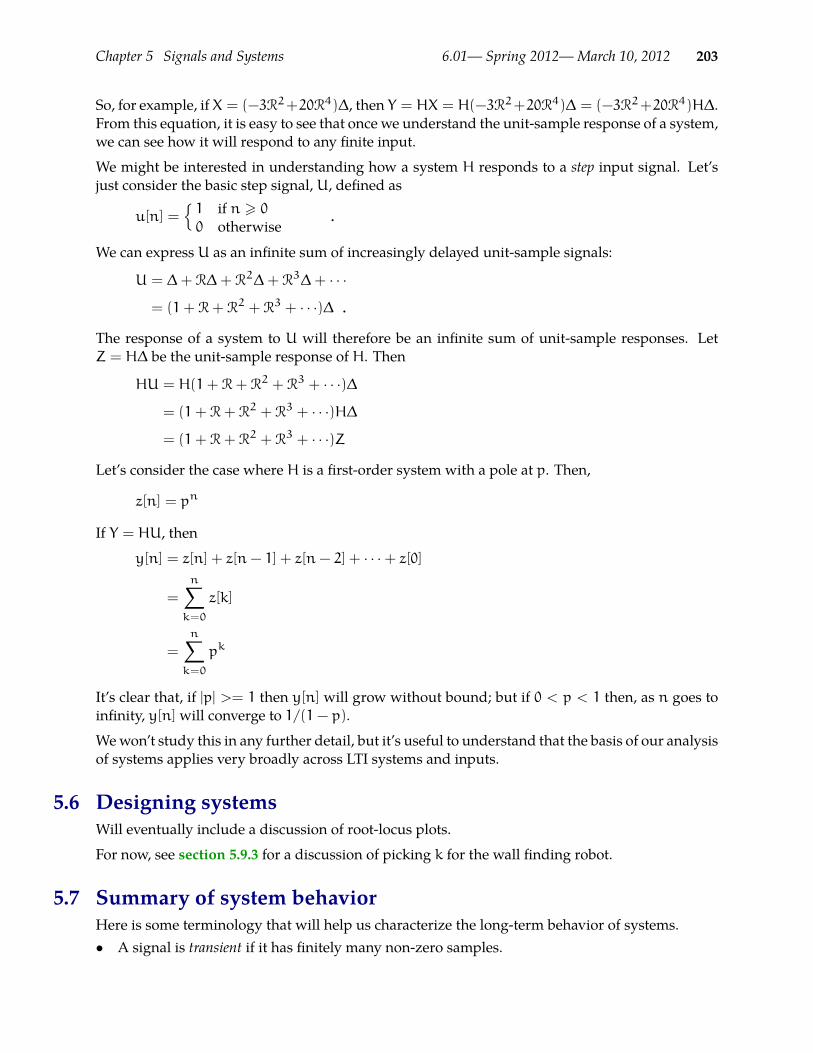
Chapter 5 Signals and Systems 6.01— Spring 2012—March 10, 2012 203
So, for example, ifX = (−3R2+20R4)∆, then Y = HX = H(−3R2+20R4)∆ = (−3R2+20R4)H∆.From this equation, it is easy to see that once we understand the unit-sample response of a system,we can see how it will respond to any finite input.
We might be interested in understanding how a system H responds to a step input signal. Let’sjust consider the basic step signal, U, defined as
u[n] =1 if n > 00 otherwise
.
We can express U as an infinite sum of increasingly delayed unit-sample signals:
U = ∆+ R∆+ R2∆+ R3∆+ · · ·
= (1+ R+ R2 + R3 + · · ·)∆ .
The response of a system to U will therefore be an infinite sum of unit-sample responses. LetZ = H∆ be the unit-sample response of H. Then
HU = H(1+ R+ R2 + R3 + · · ·)∆
= (1+ R+ R2 + R3 + · · ·)H∆
= (1+ R+ R2 + R3 + · · ·)Z
Let’s consider the case where H is a first-order system with a pole at p. Then,
z[n] = pn
If Y = HU, then
y[n] = z[n] + z[n− 1] + z[n− 2] + · · ·+ z[0]
=
n∑k=0
z[k]
=
n∑k=0
pk
It’s clear that, if |p| >= 1 then y[n] will grow without bound; but if 0 < p < 1 then, as n goes toinfinity, y[n] will converge to 1/(1− p).
Wewon’t study this in any further detail, but it’s useful to understand that the basis of our analysisof systems applies very broadly across LTI systems and inputs.
5.6 Designing systemsWill eventually include a discussion of root-locus plots.
For now, see section 5.9.3 for a discussion of picking k for the wall finding robot.
5.7 Summary of system behaviorHere is some terminology that will help us characterize the long-term behavior of systems.• A signal is transient if it has finitely many non-zero samples.
Chapter 5 Signals and Systems 6.01— Spring 2012—March 10, 2012 204
• Otherwise, it is persistent.• A signal is bounded if there is exist upper and lower bound values such that the samples of the
signal never exceed those bounds; item otherwise it is unbounded.
Now, using those terms, here is what we can say about system behavior.• A transient input to an acyclic (feed-forward) system results in a transient output.• A transient input to a cyclic (feed-back) system results in a persistent output.• The poles of a system are the roots of the denominator polynomial of the system function in1/R.
• The dominant pole is the pole with the largest magnitude.• If the dominant pole has magnitude > 1, then in response to a bounded input, the output
signal will be unbounded.• If the dominant pole has magnitude < 1, then in response to a bounded input, the output
signal will be bounded; in response to a transient input, the output signal will converge to 0.• If the dominant pole has magnitude 1, then in response to a bounded input, the output signal
will be bounded; in response to a transient input, it will converge to some constant value.• If the dominant pole is real and positive, then in response to a transient input, the signal will,
after finitely many steps, begin to increase or decrease monotonically.• If the dominant pole is real and negative, then in response to a transient input, the signal will,
after finitely many steps, begin to alternate signs.• If the dominant pole is complex, then in response to a transient input, the signal will, after
finitely many steps, begin to be periodic, with a period of 2π/Ω, whereΩ is the ’angle’ of thepole.
5.8 Signals and systems in Python
5.8.1 SignalsSignals are infinite sequences of values, so they can never be represented explicitly as a collection ofsamples. Instead, we develop a Python class for representing signals as combinations of primitivesignals. The Python Signal class is an abstract superclass: you should not make instances ofSignal directly, but instead use it as a basis for building subclasses. The Signal class providesmethods for representing a signal, for graphically depicting a signal, and for combining signals toproduce new signals.
Any signal can be thought of as being an infinite sequence of sample values. Thus, in the Signalclass, a signal is represented as a procedure that can be called with any time index; it returns thevalue of the signal at that index. Specifically, Signal assumes that every instance has a methodcalled sample, which takes time index, n, and returns the value of the signal at time n. Thus,subclasses of Signalmay be constructed, each with the samplemethod implemented to producedifferent signals, as appropriate.
A method plot(self, start=0, end=100, newWindow=’...’, color=’blue’) is also de-fined for all signals. It plots the signal from start to end, which should be integers. If newWindowis specified, it is a string usef for the title of the newwindow for this plot; if color is specified, it asa string specifying the color of the new curve to be added to the plot. The parameters start, end,

Chapter 5 Signals and Systems 6.01— Spring 2012—March 10, 2012 205
newWindow and color all have reasonable default arguments, so you can just specify the ones youneed.
5.8.1.1 Primitive signalsTwoprimitive signals are the unit sample signal and the step signal. They are defiend as subclassesof Signal. When defining a subclass of signals, it is only necessary to specify the samplemethod,which provides a way to determine the value of the signal at a given step n.
The UnitSample signal has value 1 at time 0 and value 0 at all other times:
class UnitSampleSignal(Signal):def sample(self, n):
if n == 0:return 1
else:return 0
The StepSignal has value 0 at any time index less than 0 and value 1 otherwise.
We can define a class of primitive signals that always have a constant value, c. This class requiresan __init__method to specify the value of c.
class ConstantSignal(Signal):def __init__(self, c):
self.c = cdef sample(self, n):
return self.c
Exercise 5.10. In the context of the whole system of primitive signals and combinations,would it suffice to have a single constant signal, with value 1 at all samples,instead of this whole set of constant signals for all possible c?
Somewhat more interesting is a sinusoidal signal; we implement this with a CosineSignal class,whose constructor takes a frequency omega and a phase phase:
class CosineSignal(Signal):def __init__(self, omega = 1, phase = 0):
self.omega = omegaself.phase = phase
def sample(self, n):return math.cos(self.omega * n + self.phase)
Sometimes we will want to make a signal out of previously-recorded data, or provide an explicittest pattern that is tedious to construct out of primitives. For these purposes, we provide a classof signals that supplies a list of values for samples within a given range. The ListSignal classtakes a list of samples at initialization time, which are interpreted as the sample values starting atstep 0. The value of the signal at all steps for which a value is not supplied is 0.

Chapter 5 Signals and Systems 6.01— Spring 2012—March 10, 2012 206
5.8.2 Combined signalsWe can construct new signals from primitives using Python implementations of our signal algebraoperators.
The class SummedSignal takes two signals, s1 and s2, at initialization time and represents a newsignal that is the sum of those signals. Note that this class is lazy: when the signal is created, noaddition happens; values are only added when a sample of the summed signal is requested.
The class ScaledSignal takes a signal s and a constant c at initialization time and represents anew signal whose sample values are the sample values of the original signal multiplied by c.
The class R takes a signal s at initialization time and represents a new Signalwhose samples aredelayed by one time step; that is, the value at time n of the new signal is the value at time n− 1 ofthe old signal.
The class Rn takes a signal s at initialization time and represents a new Signal whose samplesare delayed by n steps.
Exercise 5.11. Is the Rn class really necessary? If you wanted to take a signal s and createa new signal that was s delayed by 10 steps, how could you do it withoutRn? Is there a good reason to make Rn, anyway?
5.8.3 Transduced signalsThe Pythonmodule tsdefines a subclass of Signal called TransducedSignal, with initializationmethod:
def __init__(self, s, m):self.s = sself.m = m
The s argument is a signal and the m argument is a state machine. The transduced signal is thesignal that results from running the state machine m’s transduce method on the signal s.
5.8.4 ExampleWecan put all these pieces together. Imagine that youwanted to construct a signal out of some stepfunctions, then feed it into a system that you specified by composing primitive system functions,and plot the output. Here is how you could do that.
First, import the relevant modules.
import lib601.sf as sfimport lib601.sig as sigimport lib601.ts as ts
Now, make a signal.
Chapter 5 Signals and Systems 6.01— Spring 2012—March 10, 2012 207
x = 2 * sig.Rn(sig.StepSignal(), 3) + \-7 * sig.Rn(sig.StepSignal(), 7) + \0.2 * sig.Rn(sig.StepSignal(), 10)
And a system function
sysFun = sf.FeedbackSubtract(sf.Cascade(sf.R(), sf.R()),sf.Gain(.3))
Convert the system function first into a difference equation, and then into a state machine, speci-fying two previous inputs and two previous outputs.
m = sysFun.differenceEquation().stateMachine([2, 3], [5, 7])
Create the output signal resulting from transforming signal x by system m:
y = ts.TransducedSignal(x, m)
And plot the result!
y.plot()
Of course, you can do this all with one expression, if you like:
ts.TransducedSignal(2 * sig.Rn(sig.StepSignal(), 3) + \-7 * sig.Rn(sig.StepSignal(), 7) + \
0.2 * sig.Rn(sig.StepSignal(), 10),sf.FeedbackSubtract(sf.Cascade(sf.R(), sf.R()),
sf.Gain(.3)).\differenceEquation().stateMachine([2, 3], [5, 7])).plot()
5.9 Worked Examples
5.9.1 Specifying difference equationsHere are some examples of LTI systems and the way they would be described as difference equa-tions. It’s useful to pay careful attention to the specification of the coefficients. As a reminder,here’s the general form.
y[n] = c0 y[n− 1] + c1 y[n− 2] + . . .+ ck−1 y[n− k]
+ d0 x[n] + d1 x[n− 1] + . . .+ dj x[n− j]
• Output at step n is 3 times the input at step n:
y[n] = 3x[n]
dCoeffs: 3, cCoeffs: none• Output at step n is the input at step n− 1:
y[n] = x[n− 1]
dCoeffs: 0, 1, cCoeffs: none

Chapter 5 Signals and Systems 6.01— Spring 2012—March 10, 2012 208
• Output at step n is 2 times the input at step n− 2:
y[n] = 2x[n− 2]
dCoeffs: 0, 0, 2, cCoeffs: none• Output at step n is 2 times the output at step n− 1:
y[n] = 2y[n− 1]
dCoeffs: none, cCoeffs: 2• Output at step n is the input at step n− 1 plus the output at step n− 2:
y[n] = x[n− 1] + y[n− 2]
dCoeffs: 0, 1, cCoeffs: 0, 1
5.9.2 Difference equations and block diagramsLet H represent a system whose input is a signal X and whose output is a signal Y. The system H
is defined by the following difference equations:
y[n] = x[n] + z[n]
z[n] = y[n− 1] + z[n− 1]
Start by finding an operator equation.
Y = X+ Z
Z = RY + RZ
Now, we use the second equation to find an expression for Z:
Z =RY
1− R
and substitute that into the first equation, and solve for Y:
Y = X+RY
1− R
(1− R)Y = (1− R)X+ RY
(1− 2R)Y = (1− R)X
Y =1− R
1− 2RX
Part a. Which of the following systems are valid representations of H? (Remember that there canbe multiple “equivalent” representations for a system.)
+ +
R R2 −1
X Y
equivalent to H (yes/no)? YES

Chapter 5 Signals and Systems 6.01— Spring 2012—March 10, 2012 209
Find operator equations here; start by naming the signal that’s flowing between the two adders.Let’s call itW.
Y =W − RW
W = X+ 2RW
Now, rewrite the first equation as
Y = (1− R)W
And the second one as
W =X
1− 2R
Then, combine them to get
Y = (1− R)X
1− 2R
=1− R
1− 2RX
Showing that this system is the same as H.
+ +
R R2 2
X Y
equivalent to H (yes/no)? NO
This time, let’s name the signal that’s flowing between the two addersA. Now, we have equations
Y = A+ 2RY
A = X+ 2RA
Rewrite the first equation as:
Y =A
1− 2R
And the second as:
A =X
1− 2R
When we combine them, we get
Y =X
(1− 2R)(1− 2R)
which is not equivalent to the original system.
+
+
R
R
X Y
equivalent to H (yes/no)? YES
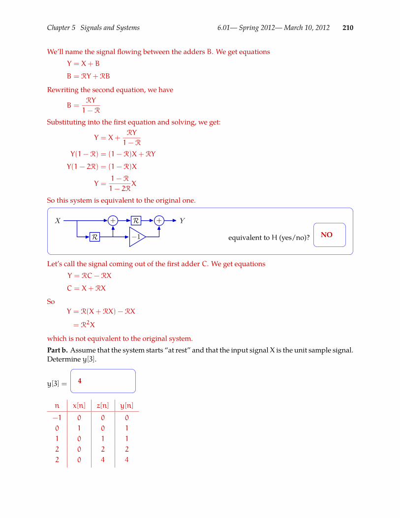
Chapter 5 Signals and Systems 6.01— Spring 2012—March 10, 2012 210
We’ll name the signal flowing between the adders B. We get equationsY = X+ B
B = RY + RB
Rewriting the second equation, we have
B =RY
1− R
Substituting into the first equation and solving, we get:
Y = X+RY
1− R
Y(1− R) = (1− R)X+ RY
Y(1− 2R) = (1− R)X
Y =1− R
1− 2RX
So this system is equivalent to the original one.
+ +
R
R
−1
X Y
equivalent to H (yes/no)? NO
Let’s call the signal coming out of the first adder C. We get equationsY = RC− RX
C = X+ RX
SoY = R(X+ RX) − RX
= R2X
which is not equivalent to the original system.Part b. Assume that the system starts “at rest” and that the input signalX is the unit sample signal.Determine y[3].
y[3] = 4
n x[n] z[n] y[n]
−1 0 0 0
0 1 0 1
1 0 1 1
2 0 2 2
2 0 4 4
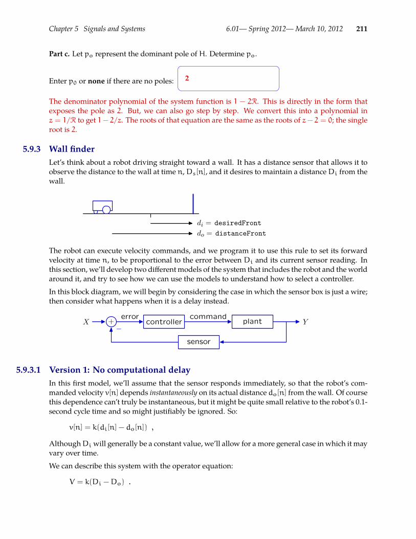
Chapter 5 Signals and Systems 6.01— Spring 2012—March 10, 2012 211
Part c. Let po represent the dominant pole of H. Determine po.
Enter p0 or none if there are no poles: 2
The denominator polynomial of the system function is 1 − 2R. This is directly in the form thatexposes the pole as 2. But, we can also go step by step. We convert this into a polynomial inz = 1/R to get 1− 2/z. The roots of that equation are the same as the roots of z− 2 = 0; the singleroot is 2.
5.9.3 Wall finderLet’s think about a robot driving straight toward a wall. It has a distance sensor that allows it toobserve the distance to the wall at time n,Ds[n], and it desires to maintain a distanceDi from thewall.
di = desiredFrontdo = distanceFront
The robot can execute velocity commands, and we program it to use this rule to set its forwardvelocity at time n, to be proportional to the error between Di and its current sensor reading. Inthis section, we’ll develop two differentmodels of the system that includes the robot and theworldaround it, and try to see how we can use the models to understand how to select a controller.
In this block diagram, we will begin by considering the case in which the sensor box is just a wire;then consider what happens when it is a delay instead.
controller plant
sensor
+X Yerror command
−
5.9.3.1 Version 1: No computational delayIn this first model, we’ll assume that the sensor responds immediately, so that the robot’s com-manded velocity v[n] depends instantaneously on its actual distance do[n] from the wall. Of coursethis dependence can’t truly be instantaneous, but it might be quite small relative to the robot’s 0.1-second cycle time and so might justifiably be ignored. So:
v[n] = k(di[n] − do[n]) ,
AlthoughDiwill generally be a constant value, we’ll allow for amore general case in which it mayvary over time.
We can describe this system with the operator equation:
V = k(Di −Do) .
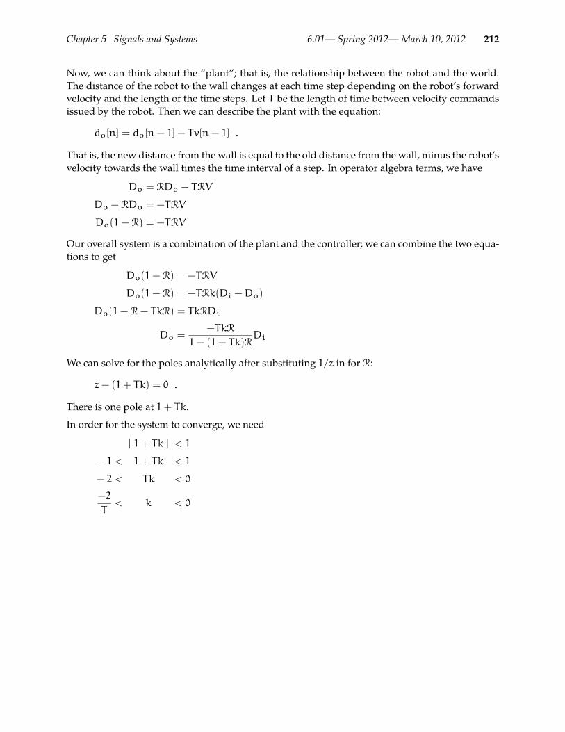
Chapter 5 Signals and Systems 6.01— Spring 2012—March 10, 2012 212
Now, we can think about the “plant”; that is, the relationship between the robot and the world.The distance of the robot to the wall changes at each time step depending on the robot’s forwardvelocity and the length of the time steps. Let T be the length of time between velocity commandsissued by the robot. Then we can describe the plant with the equation:
do[n] = do[n− 1] − Tv[n− 1] .
That is, the new distance from the wall is equal to the old distance from the wall, minus the robot’svelocity towards the wall times the time interval of a step. In operator algebra terms, we have
Do = RDo − TRV
Do − RDo = −TRV
Do(1− R) = −TRV
Our overall system is a combination of the plant and the controller; we can combine the two equa-tions to get
Do(1− R) = −TRV
Do(1− R) = −TRk(Di −Do)
Do(1− R− TkR) = TkRDi
Do =−TkR
1− (1+ Tk)RDi
We can solve for the poles analytically after substituting 1/z in for R:
z− (1+ Tk) = 0 .
There is one pole at 1+ Tk.
In order for the system to converge, we need
| 1+ Tk | < 1
− 1 < 1+ Tk < 1
− 2 < Tk < 0
−2
T< k < 0
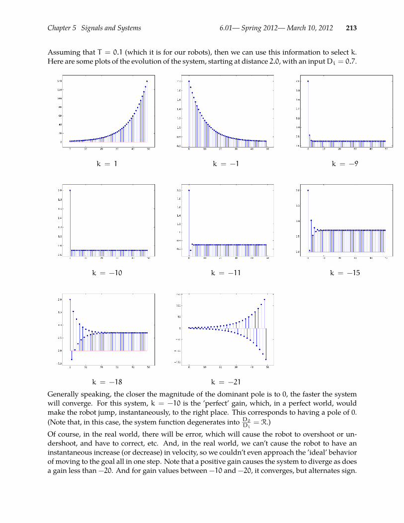
Chapter 5 Signals and Systems 6.01— Spring 2012—March 10, 2012 213
Assuming that T = 0.1 (which it is for our robots), then we can use this information to select k.Here are some plots of the evolution of the system, starting at distance 2.0, with an inputDi = 0.7.
k = 1 k = −1 k = −9
k = −10 k = −11 k = −15
k = −18 k = −21
Generally speaking, the closer the magnitude of the dominant pole is to 0, the faster the systemwill converge. For this system, k = −10 is the ’perfect’ gain, which, in a perfect world, wouldmake the robot jump, instantaneously, to the right place. This corresponds to having a pole of 0.(Note that, in this case, the system function degenerates into D0Di = R.)Of course, in the real world, there will be error, which will cause the robot to overshoot or un-dershoot, and have to correct, etc. And, in the real world, we can’t cause the robot to have aninstantaneous increase (or decrease) in velocity, so we couldn’t even approach the ’ideal’ behaviorof moving to the goal all in one step. Note that a positive gain causes the system to diverge as doesa gain less than −20. And for gain values between −10 and −20, it converges, but alternates sign.

Chapter 5 Signals and Systems 6.01— Spring 2012—March 10, 2012 214
Here is what is called a root-locus plot. It shows how the poles of the system (in this case just onepole) move in the complex plane as we vary parameter k. In this figure, we varied k from −25 to+10. The corresponding poles are plotted in different colors, starting with red corresponding tok = −25 through violet corresponding to k = +10. First, we can easily see that for any value ofk, the pole is on the real line. Then, we observe that for the lowest values of k, the pole is outsidethe unit circle (drawn in dark black, any value inside it has magnitude less than 1), and will causedivergence, and for the highest values of k it is also outside the unit circle and will also diverge.
5.9.3.2 Model 2: A delay in the sensorNow, we’ll consider a version of the problem in which there is a delay in the sensor, so that thecommanded velocity v[n] depends on the distance at the previous time step, do[n− 1], rather thanon do[n].
v[n] = k(di[n] − do[n− 1]) ,
We can describe this system with the operator equation:
V = k(Di − RDo) .
We’ll leave the model of the plant as it was above (but note that in a real situation, there might beadditional delays in the plant, as well as, or instead of, the delay we’re modeling in the controller).
Do(1− R) = −TRV .
Our overall system is a combination of the plant and the controller; we can combine the two equa-tions to get
Do(1− R) = −TRV
Do(1− R) = −TRk(Di − RDo)
Do(1− R− TkR2) = −TkRDi
Do =−TkR
1− R− TkR2Di
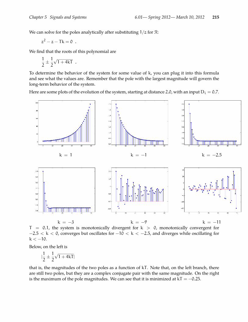
Chapter 5 Signals and Systems 6.01— Spring 2012—March 10, 2012 215
We can solve for the poles analytically after substituting 1/z for R:
z2 − z− Tk = 0 .
We find that the roots of this polynomial are1
2± 12
√1+ 4kT .
To determine the behavior of the system for some value of k, you can plug it into this formulaand see what the values are. Remember that the pole with the largest magnitude will govern thelong-term behavior of the system.
Here are some plots of the evolution of the system, starting at distance 2.0, with an inputDi = 0.7.
k = 1 k = −1 k = −2.5
k = −3 k = −9 k = −11 WhenT = 0.1, the system is monotonically divergent for k > 0, monotonically convergent for−2.5 < k < 0, converges but oscillates for −10 < k < −2.5, and diverges while oscillating fork < −10.
Below, on the left is
|1
2± 12
√1+ 4kT |
that is, the magnitudes of the two poles as a function of kT . Note that, on the left branch, thereare still two poles, but they are a complex conjugate pair with the same magnitude. On the rightis the maximum of the pole magnitudes. We can see that it is minimized at kT = −0.25.

Chapter 5 Signals and Systems 6.01— Spring 2012—March 10, 2012 216
-1.0 -0.5 0.5 1.0kt
0.5
1.0
1.5
PoleMags
-1.0 -0.5 0.5 1.0kt
0.5
1.0
1.5
magDomPole
Magnitudes of both poles Magnitude of dominant pole
Here is a root-locus plot for this system. It shows how the poles of the systemmove in the complexplane as we vary parameter k. In this figure, we varied k from −20 to +10. The correspondingpoles are plotted in different colors, starting with red corresponding to k = −20 through violetcorresponding to k = +10. There are two red points, corresponding to the conjugate pair ofcomplex poles arising when k = −20. This system is unstable, because the magnitudes of thosecomplex poles are greater than 1 (outside the unit circle). Aswe increase k, these polesmove down;that is, their real part stays constant and the imaginary part decreases, untilwe reach complex poles(greenish on the plot) that are stable. Finally, these two polesmeet on the real line: one ’turns’ rightas k increases and one ’turns’ left. Now, we have two real poles, one of which is closer to the unitcircle than the other. As soon as the positive real pole is equal to 1 then the system will begin toturn unstable again (even though the other pole is still inside the unit circle. This, for k = 10, thesystem is unstable (eventually diverging monotonically) because the largest pole is positive andoutside the unit circle.
5.9.4 Cool difference equationsNewton’s law of cooling states that: the rate of change of the temperature of an object is propor-tional to the difference between its own temperature and the temperature of its surroundings.
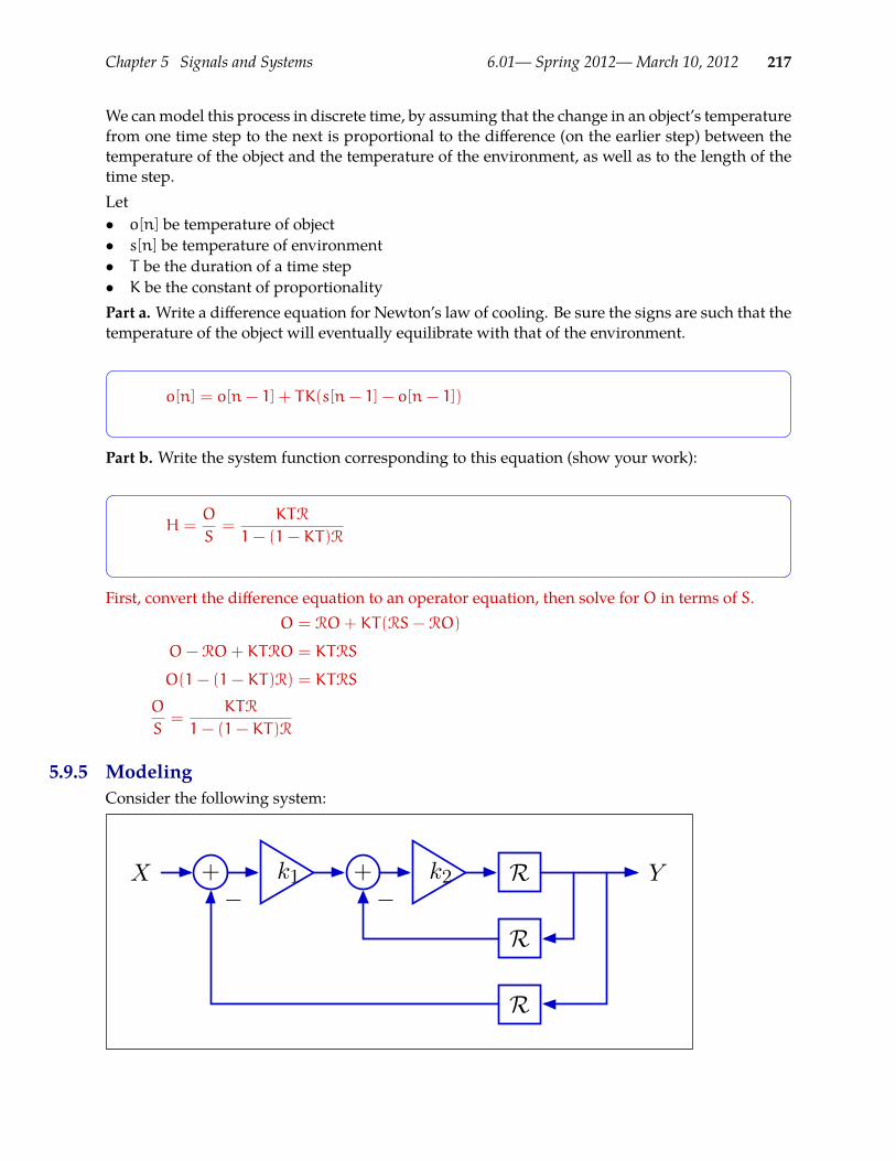
Chapter 5 Signals and Systems 6.01— Spring 2012—March 10, 2012 217
We canmodel this process in discrete time, by assuming that the change in an object’s temperaturefrom one time step to the next is proportional to the difference (on the earlier step) between thetemperature of the object and the temperature of the environment, as well as to the length of thetime step.Let• o[n] be temperature of object• s[n] be temperature of environment• T be the duration of a time step• K be the constant of proportionalityPart a. Write a difference equation for Newton’s law of cooling. Be sure the signs are such that thetemperature of the object will eventually equilibrate with that of the environment.
o[n] = o[n− 1] + TK(s[n− 1] − o[n− 1])
Part b. Write the system function corresponding to this equation (show your work):
H =O
S=
KTR
1− (1− KT)R
First, convert the difference equation to an operator equation, then solve for O in terms of S.O = RO+ KT(RS− RO)
O− RO+ KTRO = KTRS
O(1− (1− KT)R) = KTRS
O
S=
KTR
1− (1− KT)R
5.9.5 ModelingConsider the following system:
R
R
R
+ +k1 k2X Y− −
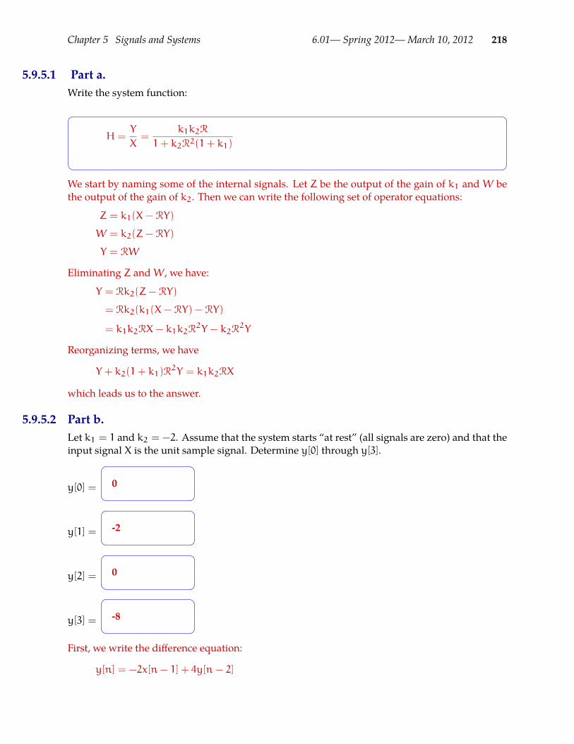
Chapter 5 Signals and Systems 6.01— Spring 2012—March 10, 2012 218
5.9.5.1 Part a.Write the system function:
H =Y
X=
k1k2R
1+ k2R2(1+ k1)
We start by naming some of the internal signals. Let Z be the output of the gain of k1 andW bethe output of the gain of k2. Then we can write the following set of operator equations:
Z = k1(X− RY)
W = k2(Z− RY)
Y = RW
Eliminating Z andW, we have:
Y = Rk2(Z− RY)
= Rk2(k1(X− RY) − RY)
= k1k2RX− k1k2R2Y − k2R
2Y
Reorganizing terms, we have
Y + k2(1+ k1)R2Y = k1k2RX
which leads us to the answer.
5.9.5.2 Part b.Let k1 = 1 and k2 = −2. Assume that the system starts “at rest” (all signals are zero) and that theinput signal X is the unit sample signal. Determine y[0] through y[3].
y[0] = 0
y[1] = -2
y[2] = 0
y[3] = -8
First, we write the difference equation:
y[n] = −2x[n− 1] + 4y[n− 2]
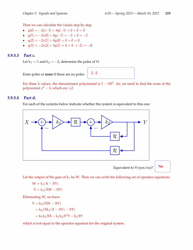
Chapter 5 Signals and Systems 6.01— Spring 2012—March 10, 2012 219
Then we can calculate the values step by step.• y[0] = −2x[−1] + 4y[−1] = 0+ 0 = 0
• y[1] = −2x[0] + 4y[−1] = −2+ 0 = −2
• y[2] = −2x[1] + 4y[0] = 0+ 0 = 0
• y[1] = −2x[2] + 4y[1] = 0+ 4 · (−2) = −8
5.9.5.3 Part c.Let k1 = 1 and k2 = −2, determine the poles of H.
Enter poles or none if there are no poles: 2, -2
For these k values, the denominator polynomial is 1 − 4R2. So, we need to find the roots of thepolynomial z2 − 4, which are ±2.
5.9.5.4 Part d.For each of the systems below indicate whether the system is equivalent to this one:
R
R
R+ +k1 k2X Y− −
Equivalent to H (yes/no)? No
Let the output of the gain of k1 beW. Then we can write the following set of operator equations:
W = k1(X− RY)
Y = k2(RW − RY)
EliminatingW, we have:
Y = k2(RW − RY)
= k2(Rk1(X− RY) − RY)
= k1k2RX− k1k2R2Y − k2RY
which is not equal to the operator equation for the original system.
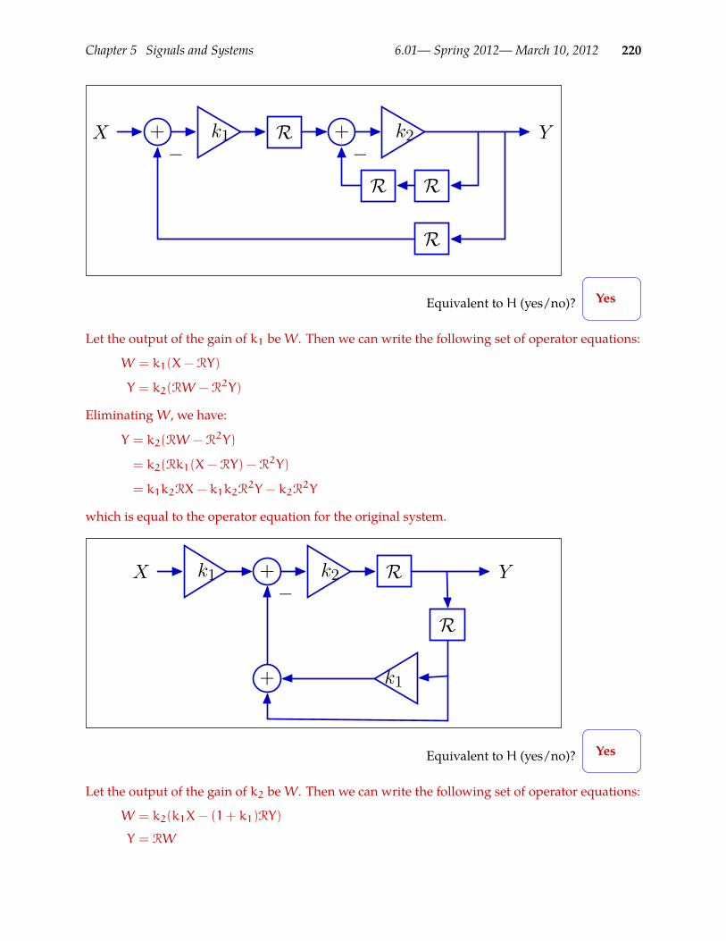
Chapter 5 Signals and Systems 6.01— Spring 2012—March 10, 2012 220
R
R
R
R
+ +k1 k2X Y− −
Equivalent to H (yes/no)? Yes
Let the output of the gain of k1 beW. Then we can write the following set of operator equations:
W = k1(X− RY)
Y = k2(RW − R2Y)
EliminatingW, we have:
Y = k2(RW − R2Y)
= k2(Rk1(X− RY) − R2Y)
= k1k2RX− k1k2R2Y − k2R
2Y
which is equal to the operator equation for the original system.
R
R
+
+
k1 k2
k1
X Y−
Equivalent to H (yes/no)? Yes
Let the output of the gain of k2 beW. Then we can write the following set of operator equations:
W = k2(k1X− (1+ k1)RY)
Y = RW

Chapter 5 Signals and Systems 6.01— Spring 2012—March 10, 2012 221
EliminatingW, we have:
Y = Rk2(k1X− (1+ k1)RY)
= k1k2RX− k1k2R2Y − k2R
2Y
which is equal to the operator equation for the original system.
R
RR
+
+
k1 k2
k1
X Y−
Equivalent to H (yes/no)? No
This is like the previous system, but with an extra delay in the feedback path, so it cannot beequivalent to the original system.
5.9.6 SM to DEHere is the definition of a class of state machines:
class Thing(SM):startState = [0, 0, 0, 0]def getNextValues(self, state, inp):
result = state[0] * 2 + state[2] * 3newState = [state[1], result, state[3], inp]return (newState, result)
1. What is the result of evaluating
Thing().transduce([1, 2, 0, 1, 3])
[0, 0, 3, 6, 6]
2. The state machine above describes the behavior of an LTI system starting at rest. Write a dif-ference equation that describes the same system as the state machine.
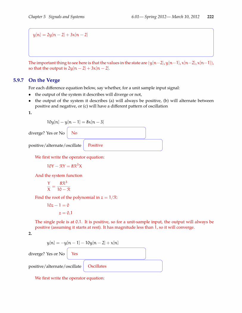
Chapter 5 Signals and Systems 6.01— Spring 2012—March 10, 2012 222
y[n] = 2y[n− 2] + 3x[n− 2]
The important thing to see here is that the values in the state are (y[n−2], y[n−1], x[n−2], x[n−1]),so that the output is 2y[n− 2] + 3x[n− 2].
5.9.7 On the VergeFor each difference equation below, say whether, for a unit sample input signal:• the output of the system it describes will diverge or not,• the output of the system it describes (a) will always be positive, (b) will alternate between
positive and negative, or (c) will have a different pattern of oscillation1.
10y[n] − y[n− 1] = 8x[n− 3]
diverge? Yes or No No
positive/alternate/oscillate Positive
We first write the operator equation:
10Y − RY = 8R3X
And the system function
Y
X=
8R3
10− R
Find the root of the polynomial in z = 1/R:
10z− 1 = 0
z = 0.1
The single pole is at 0.1. It is positive, so for a unit-sample input, the output will always bepositive (assuming it starts at rest). It has magnitude less than 1, so it will converge.
2.
y[n] = −y[n− 1] − 10y[n− 2] + x[n]
diverge? Yes or No Yes
positive/alternate/oscillate Oscillates
We first write the operator equation:
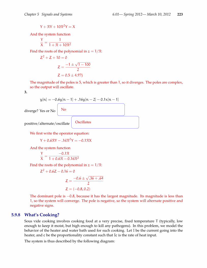
Chapter 5 Signals and Systems 6.01— Spring 2012—March 10, 2012 223
Y + RY + 10R2Y = X
And the system functionY
X=
1
1+ R+ 10R2
Find the roots of the polynomial in z = 1/R:
Z2 + Z+ 10 = 0
Z =−1±
√1− 100
2
Z = 0.5± 4.97j
The magnitude of the poles is 5, which is greater than 1, so it diverges. The poles are complex,so the output will oscillate.
3.
y[n] = −0.6y[n− 1] + .16y[n− 2] − 0.1x[n− 1]
diverge? Yes or No No
positive/alternate/oscillate Oscillates
We first write the operator equation:
Y + 0.6RY − .16R2Y = −0.1RX
And the system functionY
X=
−0.1R
1+ 0.6R− 0.16R2
Find the roots of the polynomial in z = 1/R:
Z2 + 0.6Z− 0.16 = 0
Z =−0.6±
√.36+ .64
2
Z = (−0.8, 0.2)
The dominant pole is −0.8, because it has the largest magnitude. Its magnitude is less than1, so the system will converge. The pole is negative, so the system will alternate positive andnegative signs.
5.9.8 What’s Cooking?Sous vide cooking involves cooking food at a very precise, fixed temperature T (typically, lowenough to keep it moist, but high enough to kill any pathogens). In this problem, we model thebehavior of the heater and water bath used for such cooking. Let I be the current going into theheater, and c be the proportionality constant such that Ic is the rate of heat input.The system is thus described by the following diagram:

Chapter 5 Signals and Systems 6.01— Spring 2012—March 10, 2012 224
+ +
Delay Delay
-I T
k1 k2
c
1. a. Give the system function:c
(1− k1R)(1+ k2R)
If we name the signal coming out of the first adderW, then we have operator equations
W = cI+ k1RW
T =W − k2RT
Solving, we get
W − k1RW = cI
W(1− k1R) = cI
W =cI
1− k1R
T =cI
1− k1R− k2RT
T(1− k1R) = cI− k2RT(1− k1R)
T − k1RT + k2RT − k1k2R2T = cI
T(1− k1R)(1+ k2R) = cI
T
I=
c
(1− k1R)(1+ k2R)
b. Give a difference equation for the system: t[n] =
t[n] = (k1 − k2)t[n− 1] + k1k2t[n− 2] + ci[n]
Starting with this form of the operator equation, taken from the derivation above, and thenrearranging terms
T(1− k1R) = cI− k2RT(1− k1R)
T = cI+ k1RT − k2RT(1− k1R)
We get an equation that’s easy to convert to the difference equation above.
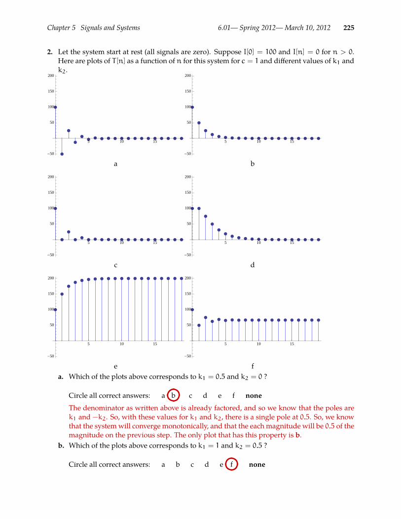
Chapter 5 Signals and Systems 6.01— Spring 2012—March 10, 2012 225
2. Let the system start at rest (all signals are zero). Suppose I[0] = 100 and I[n] = 0 for n > 0.Here are plots of T [n] as a function of n for this system for c = 1 and different values of k1 andk2.
5 10 15
-50
50
100
150
200
5 10 15
-50
50
100
150
200
a b
5 10 15
-50
50
100
150
200
5 10 15
-50
50
100
150
200
c d
5 10 15
-50
50
100
150
200
5 10 15
-50
50
100
150
200
e fa. Which of the plots above corresponds to k1 = 0.5 and k2 = 0 ?
Circle all correct answers: a b c d e f none
The denominator as written above is already factored, and so we know that the poles arek1 and −k2. So, with these values for k1 and k2, there is a single pole at 0.5. So, we knowthat the systemwill converge monotonically, and that the each magnitude will be 0.5 of themagnitude on the previous step. The only plot that has this property is b.
b. Which of the plots above corresponds to k1 = 1 and k2 = 0.5 ?
Circle all correct answers: a b c d e f none
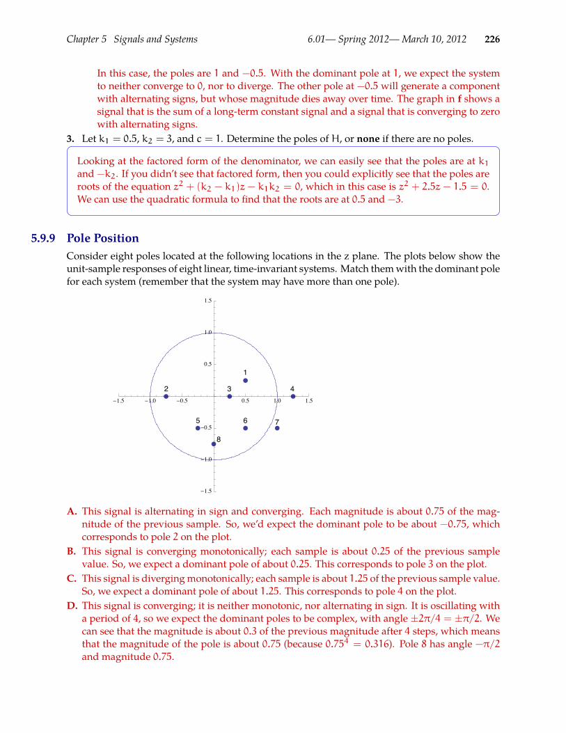
Chapter 5 Signals and Systems 6.01— Spring 2012—March 10, 2012 226
In this case, the poles are 1 and −0.5. With the dominant pole at 1, we expect the systemto neither converge to 0, nor to diverge. The other pole at −0.5 will generate a componentwith alternating signs, but whose magnitude dies away over time. The graph in f shows asignal that is the sum of a long-term constant signal and a signal that is converging to zerowith alternating signs.
3. Let k1 = 0.5, k2 = 3, and c = 1. Determine the poles of H, or none if there are no poles.
Looking at the factored form of the denominator, we can easily see that the poles are at k1and −k2. If you didn’t see that factored form, then you could explicitly see that the poles areroots of the equation z2 + (k2 − k1)z − k1k2 = 0, which in this case is z2 + 2.5z − 1.5 = 0.We can use the quadratic formula to find that the roots are at 0.5 and −3.
5.9.9 Pole PositionConsider eight poles located at the following locations in the z plane. The plots below show theunit-sample responses of eight linear, time-invariant systems. Match themwith the dominant polefor each system (remember that the system may have more than one pole).
1.5 1.0 0.5 0.5 1.0 1.5
1.5
1.0
0.5
0.5
1.0
1.5
1
2 3 4
5 6 7
8
A. This signal is alternating in sign and converging. Each magnitude is about 0.75 of the mag-nitude of the previous sample. So, we’d expect the dominant pole to be about −0.75, whichcorresponds to pole 2 on the plot.
B. This signal is converging monotonically; each sample is about 0.25 of the previous samplevalue. So, we expect a dominant pole of about 0.25. This corresponds to pole 3 on the plot.
C. This signal is divergingmonotonically; each sample is about 1.25 of the previous sample value.So, we expect a dominant pole of about 1.25. This corresponds to pole 4 on the plot.
D. This signal is converging; it is neither monotonic, nor alternating in sign. It is oscillating witha period of 4, so we expect the dominant poles to be complex, with angle ±2π/4 = ±π/2. Wecan see that the magnitude is about 0.3 of the previous magnitude after 4 steps, which meansthat the magnitude of the pole is about 0.75 (because 0.754 = 0.316). Pole 8 has angle −π/2and magnitude 0.75.

Chapter 5 Signals and Systems 6.01— Spring 2012—March 10, 2012 227
E. This signal is converging and oscillating. The period seems to be 8. So, we’d expect a pole atangle ±pi/4. The magnitude is a bit tricky to estimate. It seems to get from 2 to about 0.1 in 8steps, so it’s something like 0.7. That corresponds well to pole 6.
F. This signal is converging and oscillating. The period seems to be something like 3, and themagnitude even smaller than the previous two. Pole 5 has these characteristics.
G. This signal is diverging and oscillating. It seems to have a period of about 12, which wouldmean an angle of ±π/6. The only pole on our picture with magnitude greater than 1 is at thecorrect angle, and so it must be 7.
H. Finally, we have a signal that converges and oscillates. The period seems to be 10 or 12 and therate fairly fast; pole 1 has a smaller magnitude than pole 6, and this converges faster than E, sothis must be pole 1.
5.9.10 System functionsLet H1 represent a subsystem that is part of the larger system shown below.
+ H1
RK0
X0 Y0−
The system function for the larger system can be written as
H0 =Y0
X0=
H1
1+ K0RH1.
Assume that H1 = H1B = Y1X1
as shown below.
+
R
R
KB
X1 Y1
What is the system function for H1B?
H1B =R
1− KBR2
Determine the system function H0 for the larger system when H1 = H1B.
H0 =R
1+ (K0 − KB)R2
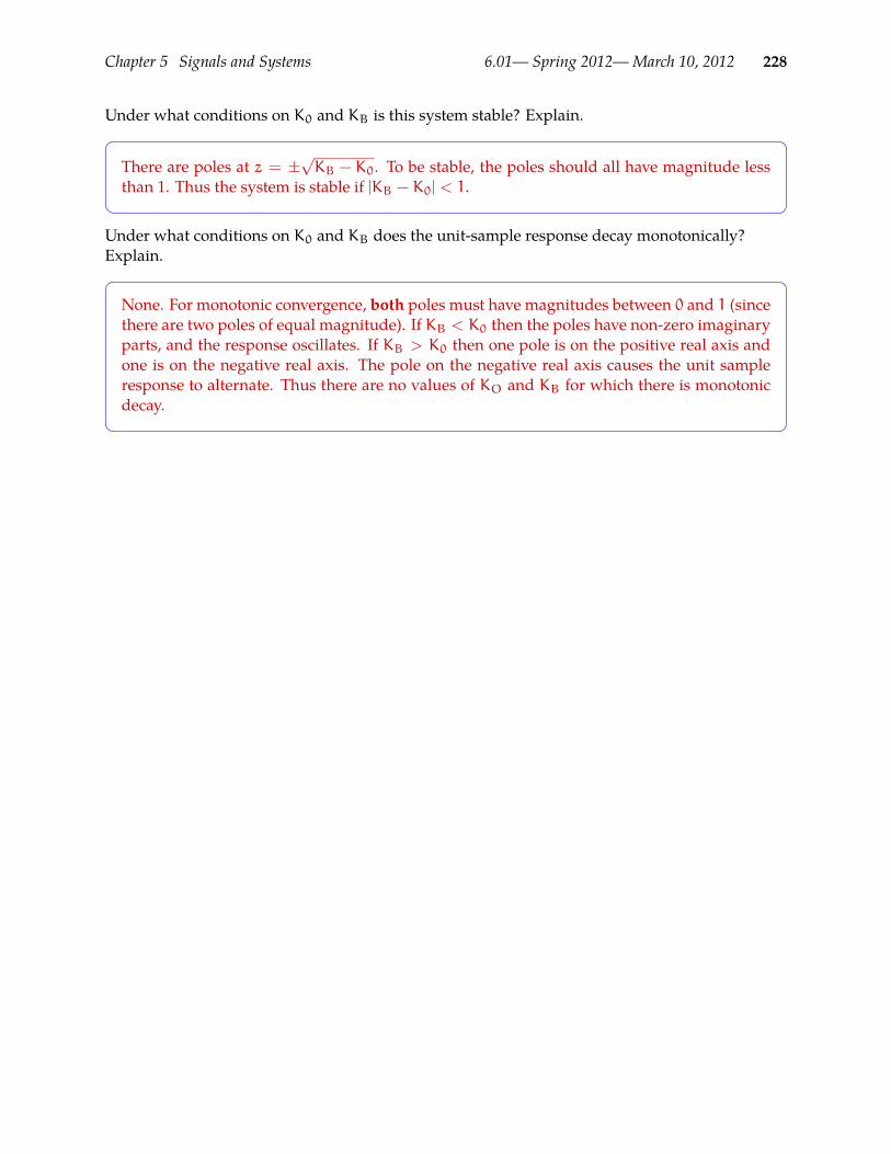
Chapter 5 Signals and Systems 6.01— Spring 2012—March 10, 2012 228
Under what conditions on K0 and KB is this system stable? Explain.
There are poles at z = ±√KB − K0. To be stable, the poles should all have magnitude less
than 1. Thus the system is stable if |KB − K0| < 1.
Under what conditions on K0 and KB does the unit-sample response decay monotonically?Explain.
None. For monotonic convergence, both poles must have magnitudes between 0 and 1 (sincethere are two poles of equal magnitude). If KB < K0 then the poles have non-zero imaginaryparts, and the response oscillates. If KB > K0 then one pole is on the positive real axis andone is on the negative real axis. The pole on the negative real axis causes the unit sampleresponse to alternate. Thus there are no values of KO and KB for which there is monotonicdecay.

Chapter 6 Circuits 6.01— Spring 2012—March 10, 2012 229
Chapter 6Circuits
6.1 What is a circuit?In conventional English, a circuit is a path or route that starts at one place and ultimately returnsto that same place. The engineering sense of the word is similar. In electronics, a circuit is a closedpath through which electrical currents can flow. The flow of electrical current through a flashlightillustrates the idea.
Three parts of the flashlight comprise the circuit: the battery, which supplies power, a bulb, whichproduces light when connected to the battery, and a switch, which can either be on (connected) oroff (disconnected). The important feature of this circuit is that electrical currents flow through itin a loop, as illustrated in the right part of the figure above.
The rules that govern the flow of electrical current are similar to the rules that govern the flow ofcertain types of fluids; and it is often helpful to draw analogies between these flows. The followingfigure illustrates the flow of blood through the human circulatory system.
heart
liver
intestines
kidneys
trunk and legs
head and arms
lungs
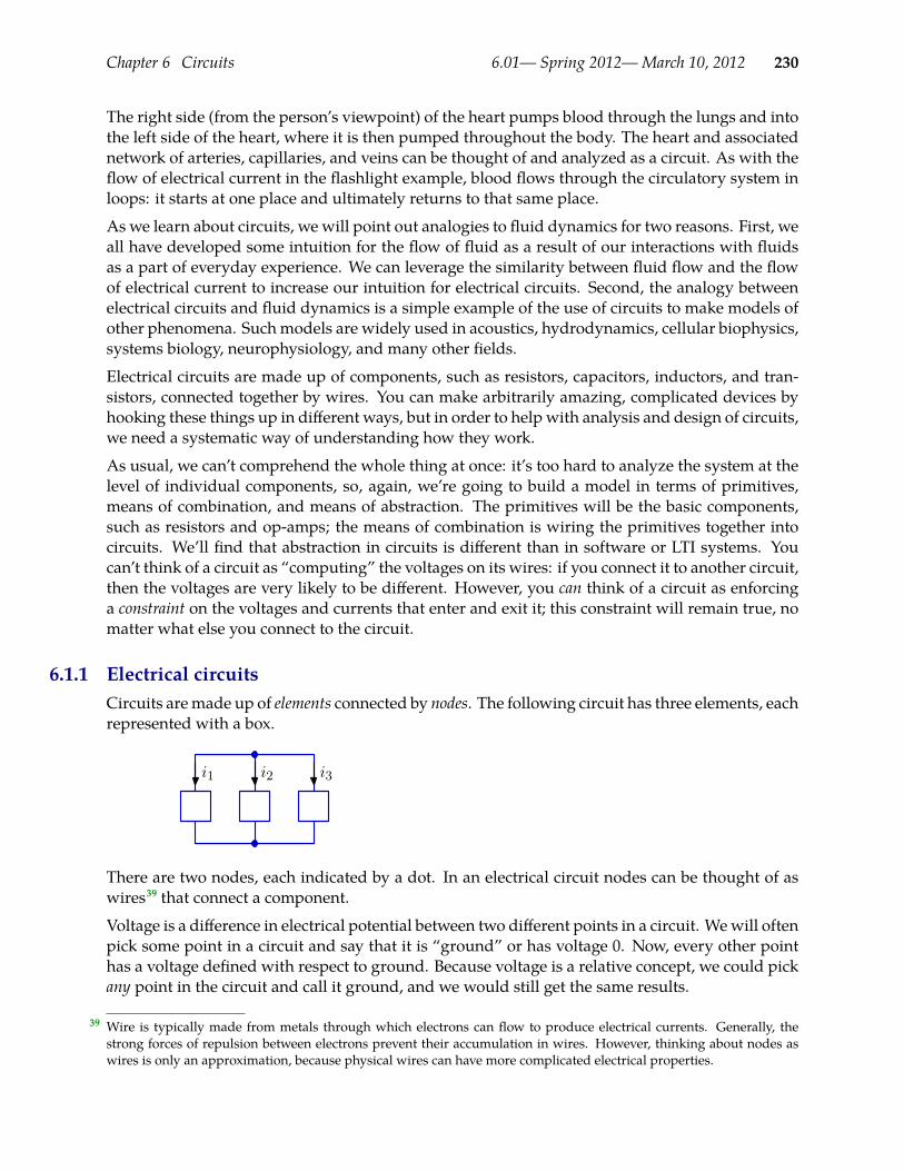
Chapter 6 Circuits 6.01— Spring 2012—March 10, 2012 230
The right side (from the person’s viewpoint) of the heart pumps blood through the lungs and intothe left side of the heart, where it is then pumped throughout the body. The heart and associatednetwork of arteries, capillaries, and veins can be thought of and analyzed as a circuit. As with theflow of electrical current in the flashlight example, blood flows through the circulatory system inloops: it starts at one place and ultimately returns to that same place.
As we learn about circuits, we will point out analogies to fluid dynamics for two reasons. First, weall have developed some intuition for the flow of fluid as a result of our interactions with fluidsas a part of everyday experience. We can leverage the similarity between fluid flow and the flowof electrical current to increase our intuition for electrical circuits. Second, the analogy betweenelectrical circuits and fluid dynamics is a simple example of the use of circuits to make models ofother phenomena. Suchmodels are widely used in acoustics, hydrodynamics, cellular biophysics,systems biology, neurophysiology, and many other fields.
Electrical circuits are made up of components, such as resistors, capacitors, inductors, and tran-sistors, connected together by wires. You can make arbitrarily amazing, complicated devices byhooking these things up in different ways, but in order to help with analysis and design of circuits,we need a systematic way of understanding how they work.
As usual, we can’t comprehend the whole thing at once: it’s too hard to analyze the system at thelevel of individual components, so, again, we’re going to build a model in terms of primitives,means of combination, and means of abstraction. The primitives will be the basic components,such as resistors and op-amps; the means of combination is wiring the primitives together intocircuits. We’ll find that abstraction in circuits is different than in software or LTI systems. Youcan’t think of a circuit as “computing” the voltages on its wires: if you connect it to another circuit,then the voltages are very likely to be different. However, you can think of a circuit as enforcinga constraint on the voltages and currents that enter and exit it; this constraint will remain true, nomatter what else you connect to the circuit.
6.1.1 Electrical circuitsCircuits aremade up of elements connected by nodes. The following circuit has three elements, eachrepresented with a box.
i1 i2 i3
There are two nodes, each indicated by a dot. In an electrical circuit nodes can be thought of aswires39 that connect a component.
Voltage is a difference in electrical potential between two different points in a circuit. Wewill oftenpick some point in a circuit and say that it is “ground” or has voltage 0. Now, every other pointhas a voltage defined with respect to ground. Because voltage is a relative concept, we could pickany point in the circuit and call it ground, and we would still get the same results.
Wire is typically made from metals through which electrons can flow to produce electrical currents. Generally, the39
strong forces of repulsion between electrons prevent their accumulation in wires. However, thinking about nodes aswires is only an approximation, because physical wires can have more complicated electrical properties.
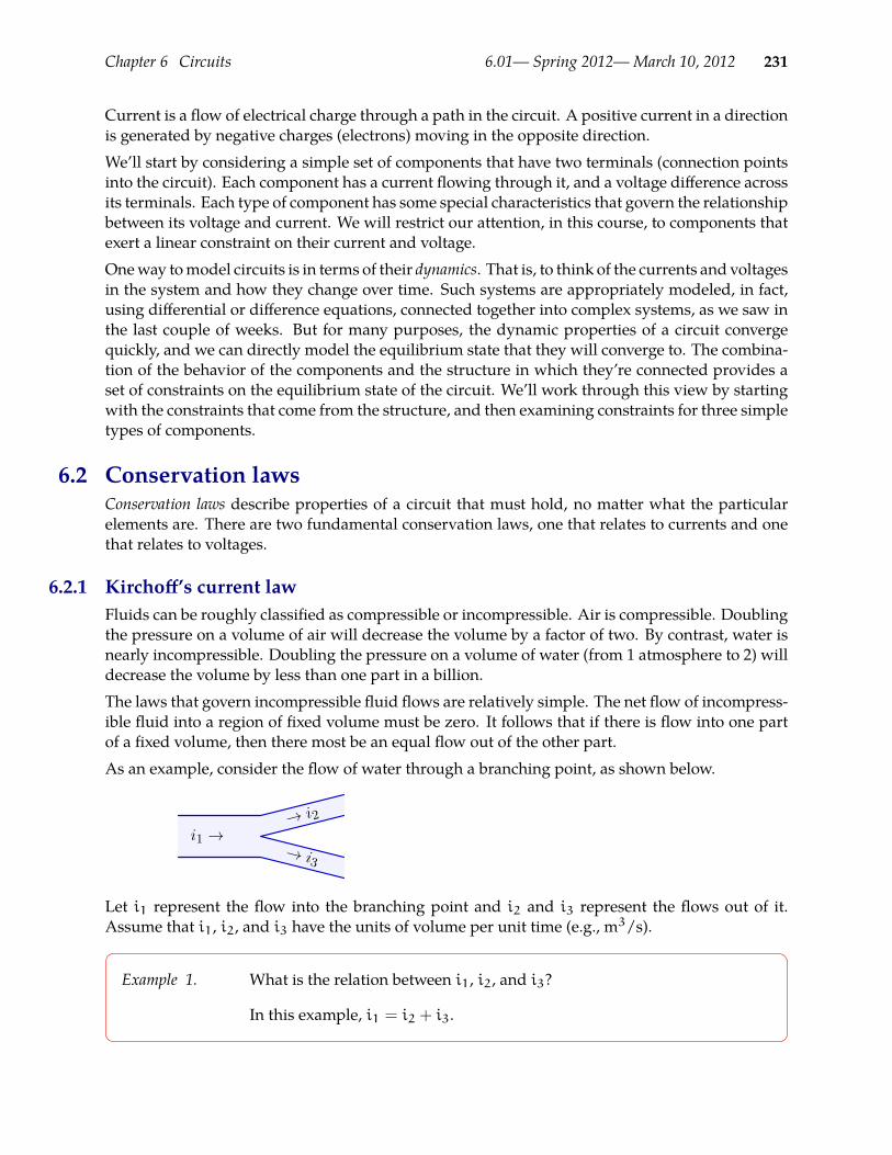
Chapter 6 Circuits 6.01— Spring 2012—March 10, 2012 231
Current is a flow of electrical charge through a path in the circuit. A positive current in a directionis generated by negative charges (electrons) moving in the opposite direction.We’ll start by considering a simple set of components that have two terminals (connection pointsinto the circuit). Each component has a current flowing through it, and a voltage difference acrossits terminals. Each type of component has some special characteristics that govern the relationshipbetween its voltage and current. We will restrict our attention, in this course, to components thatexert a linear constraint on their current and voltage.Oneway tomodel circuits is in terms of their dynamics. That is, to think of the currents and voltagesin the system and how they change over time. Such systems are appropriately modeled, in fact,using differential or difference equations, connected together into complex systems, as we saw inthe last couple of weeks. But for many purposes, the dynamic properties of a circuit convergequickly, and we can directly model the equilibrium state that they will converge to. The combina-tion of the behavior of the components and the structure in which they’re connected provides aset of constraints on the equilibrium state of the circuit. We’ll work through this view by startingwith the constraints that come from the structure, and then examining constraints for three simpletypes of components.
6.2 Conservation lawsConservation laws describe properties of a circuit that must hold, no matter what the particularelements are. There are two fundamental conservation laws, one that relates to currents and onethat relates to voltages.
6.2.1 Kirchoff’s current lawFluids can be roughly classified as compressible or incompressible. Air is compressible. Doublingthe pressure on a volume of air will decrease the volume by a factor of two. By contrast, water isnearly incompressible. Doubling the pressure on a volume of water (from 1 atmosphere to 2) willdecrease the volume by less than one part in a billion.The laws that govern incompressible fluid flows are relatively simple. The net flow of incompress-ible fluid into a region of fixed volume must be zero. It follows that if there is flow into one partof a fixed volume, then there most be an equal flow out of the other part.As an example, consider the flow of water through a branching point, as shown below.
i1 →→ i2
→ i3
Let i1 represent the flow into the branching point and i2 and i3 represent the flows out of it.Assume that i1, i2, and i3 have the units of volume per unit time (e.g., m3/s).
Example 1. What is the relation between i1, i2, and i3?
In this example, i1 = i2 + i3.

Chapter 6 Circuits 6.01— Spring 2012—March 10, 2012 232
Example 2. What if i2 represented flow in the opposite direction, as shown below?
i1 →← i2
→ i3
Now i1 + i2 = i3 or equivalently i1 = −i2 + i3.
Changing the direction of a flow variable is equivalent to changing its sign. For that reason, wethink about flowvariables as signed variables. The direction associatedwith the variable representsthe direction that results when the variable is positive. The flow is in the opposite direction if thevariable is negative. Thus, the direction that we associate with a flow is arbitrary. If we happento associate the one direction, the flow variable will be positive. If we happen to associate theopposite direction, the flow variable will be negative.
The laws for the flow of electrical current are similar to those for the flow of an incompressiblefluid. The net flow of electrical current into a nodemust be zero.
The following circuit has three elements, each represented with a box.
i1 i2 i3
There are two nodes, each indicated by a dot. The net current into or out of each of these nodes iszero. Therefore i1 + i2 + i3 = 0.
Similar current relations apply for all nodes in a circuit. Such relations are called Kirchoff’s Cur-rent Laws (KCL) and represent the first of two fundamental conservation laws for circuits.
Kirchoff’s Current Law: the sum of the currents that flow into a node is zero.
Electrical currents cannot accumulate in elements, so the current that flows into a circuit elementmust equal to the current that flows out.
i1 i2 i3
i4 i5 i6
Therefore i1 = i4, i2 = i5, and i3 = i6.
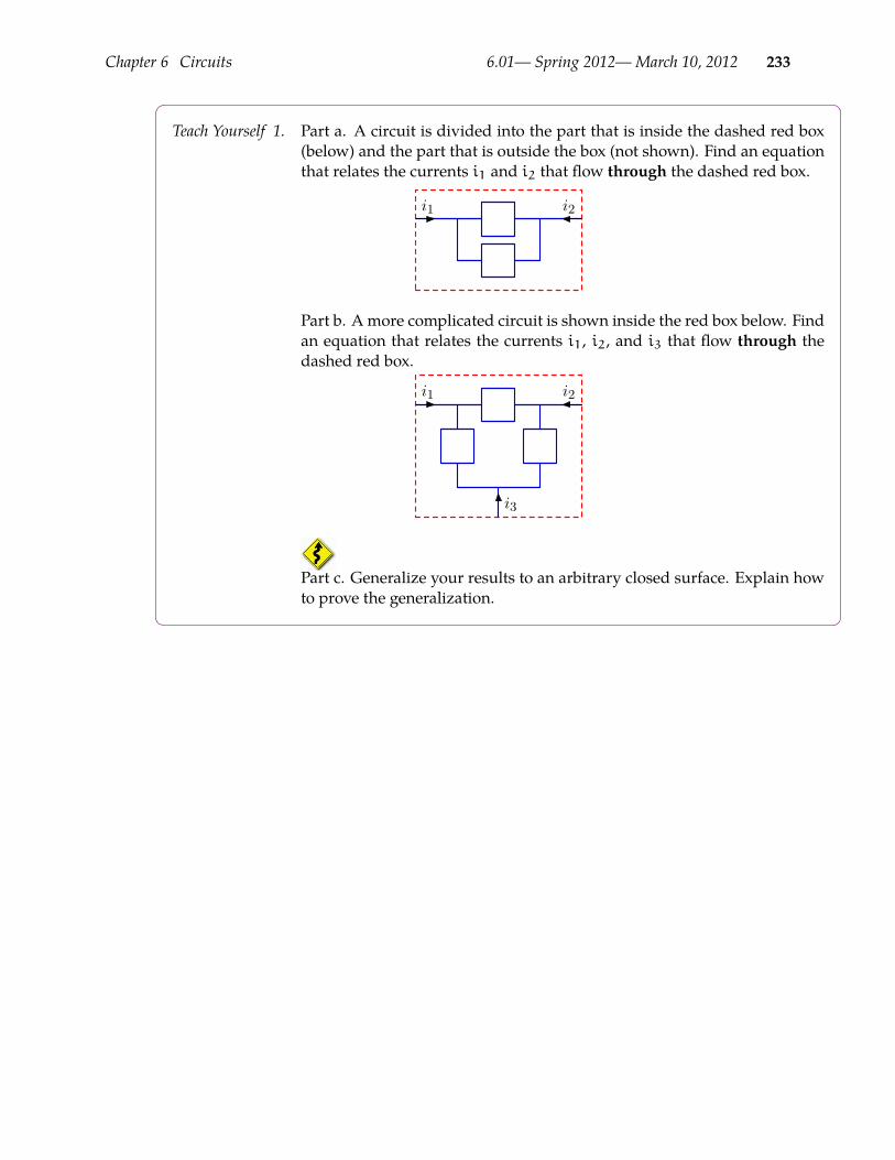
Chapter 6 Circuits 6.01— Spring 2012—March 10, 2012 233
Teach Yourself 1. Part a. A circuit is divided into the part that is inside the dashed red box(below) and the part that is outside the box (not shown). Find an equationthat relates the currents i1 and i2 that flow through the dashed red box.
i1 i2
Part b. A more complicated circuit is shown inside the red box below. Findan equation that relates the currents i1, i2, and i3 that flow through thedashed red box.
i1 i2
i3
Part c. Generalize your results to an arbitrary closed surface. Explain howto prove the generalization.
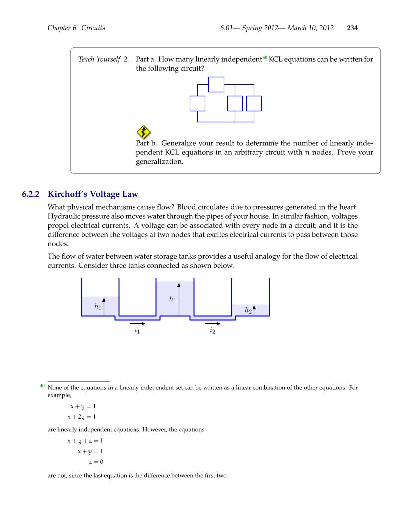
Chapter 6 Circuits 6.01— Spring 2012—March 10, 2012 234
Teach Yourself 2. Part a. Howmany linearly independent40 KCL equations can be written forthe following circuit?
Part b. Generalize your result to determine the number of linearly inde-pendent KCL equations in an arbitrary circuit with n nodes. Prove yourgeneralization.
6.2.2 Kirchoff’s Voltage LawWhat physical mechanisms cause flow? Blood circulates due to pressures generated in the heart.Hydraulic pressure alsomoves water through the pipes of your house. In similar fashion, voltagespropel electrical currents. A voltage can be associated with every node in a circuit; and it is thedifference between the voltages at two nodes that excites electrical currents to pass between thosenodes.
The flow of water between water storage tanks provides a useful analogy for the flow of electricalcurrents. Consider three tanks connected as shown below.
h0h1
h2
i1 i2
None of the equations in a linearly independent set can be written as a linear combination of the other equations. For40
example,
x+ y = 1
x+ 2y = 1
are linearly independent equations. However, the equations
x+ y+ z = 1
x+ y = 1
z = 0
are not, since the last equation is the difference between the first two.
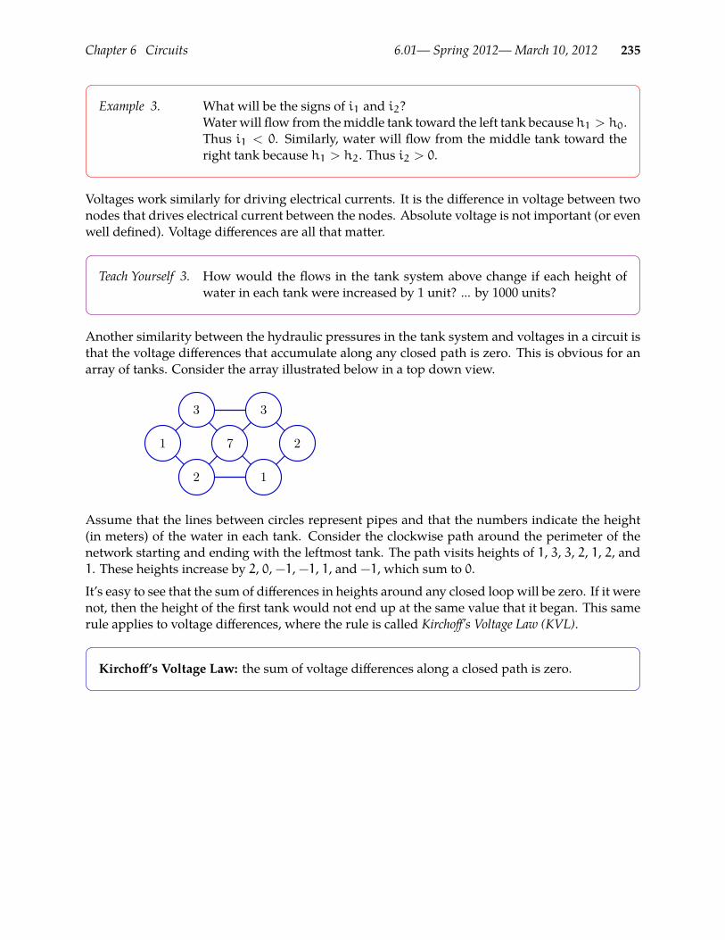
Chapter 6 Circuits 6.01— Spring 2012—March 10, 2012 235
Example 3. What will be the signs of i1 and i2?Water will flow from themiddle tank toward the left tank because h1 > h0.Thus i1 < 0. Similarly, water will flow from the middle tank toward theright tank because h1 > h2. Thus i2 > 0.
Voltages work similarly for driving electrical currents. It is the difference in voltage between twonodes that drives electrical current between the nodes. Absolute voltage is not important (or evenwell defined). Voltage differences are all that matter.
Teach Yourself 3. How would the flows in the tank system above change if each height ofwater in each tank were increased by 1 unit? ... by 1000 units?
Another similarity between the hydraulic pressures in the tank system and voltages in a circuit isthat the voltage differences that accumulate along any closed path is zero. This is obvious for anarray of tanks. Consider the array illustrated below in a top down view.
1
3
2
7
3
1
2
Assume that the lines between circles represent pipes and that the numbers indicate the height(in meters) of the water in each tank. Consider the clockwise path around the perimeter of thenetwork starting and ending with the leftmost tank. The path visits heights of 1, 3, 3, 2, 1, 2, and1. These heights increase by 2, 0, −1, −1, 1, and −1, which sum to 0.
It’s easy to see that the sum of differences in heights around any closed loop will be zero. If it werenot, then the height of the first tank would not end up at the same value that it began. This samerule applies to voltage differences, where the rule is called Kirchoff’s Voltage Law (KVL).
Kirchoff’s Voltage Law: the sum of voltage differences along a closed path is zero.

Chapter 6 Circuits 6.01— Spring 2012—March 10, 2012 236
Example 4. How many KVL equations can be written for the following circuit.
+
−v1
+
−v2
+
−v3
How many of the KVL equations are linearly independent?There are three loops through this circuit. One through the left two ele-ments yields the KVL equation −v1 + v2 = 0 or v1 = v2. One through theright two elements yields the KVL equation −v2 + v3 = 0 or v2 = v3. Onethrough the outer two elements yields the KVL equation −v1 + v3 = 0 orv1 = v3.Only two of the three KVL equations are linearly independent, since eachequation can be derived from the other two.The particularly simple solution to this circuit is that v1 = v2 = v3. Thissolution could also have been derived directly from the fact that there arejust two nodes, and therefore only one possible potential difference.
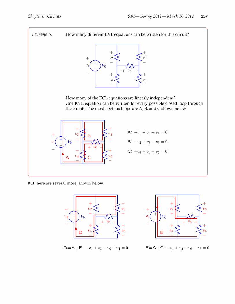
Chapter 6 Circuits 6.01— Spring 2012—March 10, 2012 237
Example 5. How many different KVL equations can be written for this circuit?
+−
V0
+
−
v1
+
−v2
+
−v3
+
−v4
+
−v5
+ −v6
How many of the KCL equations are linearly independent?One KVL equation can be written for every possible closed loop throughthe circuit. The most obvious loops are A, B, and C shown below.
A
B
C
+−
V0
+
−
v1
+
−v2
+
−v3
+
−v4
+
−v5
+ −v6
A: −v1 + v2 + v4 = 0
B: −v2 + v3 − v6 = 0
C: −v4 + v6 + v5 = 0
But there are several more, shown below.
D
+−
V0
+
−
v1
+
−v2
+
−v3
+
−v4
+
−v5
+ −v6
D=A+B: −v1 + v3 − v6 + v4 = 0
E
+−
V0
+
−
v1
+
−v2
+
−v3
+
−v4
+
−v5
+ −v6
E=A+C: −v1 + v2 + v6 + v5 = 0
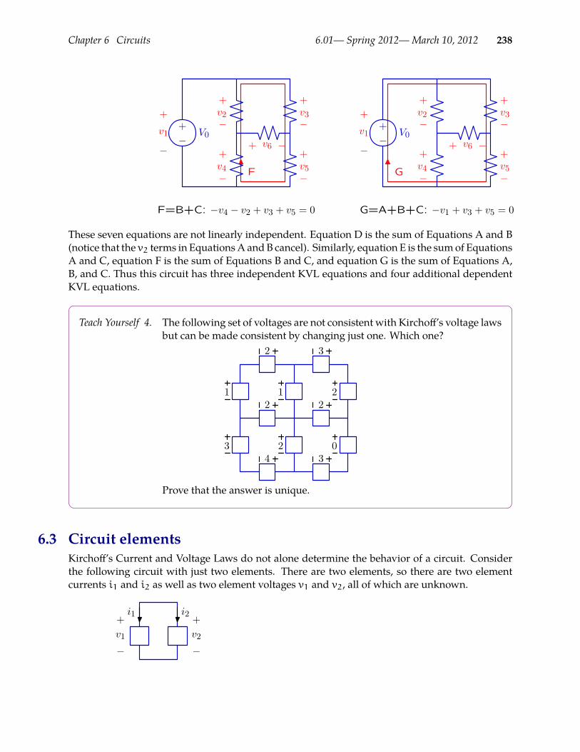
Chapter 6 Circuits 6.01— Spring 2012—March 10, 2012 238
F
+−
V0
+
−
v1
+
−v2
+
−v3
+
−v4
+
−v5
+ −v6
F=B+C: −v4 − v2 + v3 + v5 = 0
G
+−
V0
+
−
v1
+
−v2
+
−v3
+
−v4
+
−v5
+ −v6
G=A+B+C: −v1 + v3 + v5 = 0
These seven equations are not linearly independent. Equation D is the sum of Equations A and B(notice that the v2 terms in EquationsA andB cancel). Similarly, equation E is the sumof EquationsA and C, equation F is the sum of Equations B and C, and equation G is the sum of Equations A,B, and C. Thus this circuit has three independent KVL equations and four additional dependentKVL equations.
Teach Yourself 4. The following set of voltages are not consistent with Kirchoff’s voltage lawsbut can be made consistent by changing just one. Which one?
1
2
21
3
22
34
23
0
Prove that the answer is unique.
6.3 Circuit elementsKirchoff’s Current and Voltage Laws do not alone determine the behavior of a circuit. Considerthe following circuit with just two elements. There are two elements, so there are two elementcurrents i1 and i2 as well as two element voltages v1 and v2, all of which are unknown.
i1 i2+
−v1
+
−v2
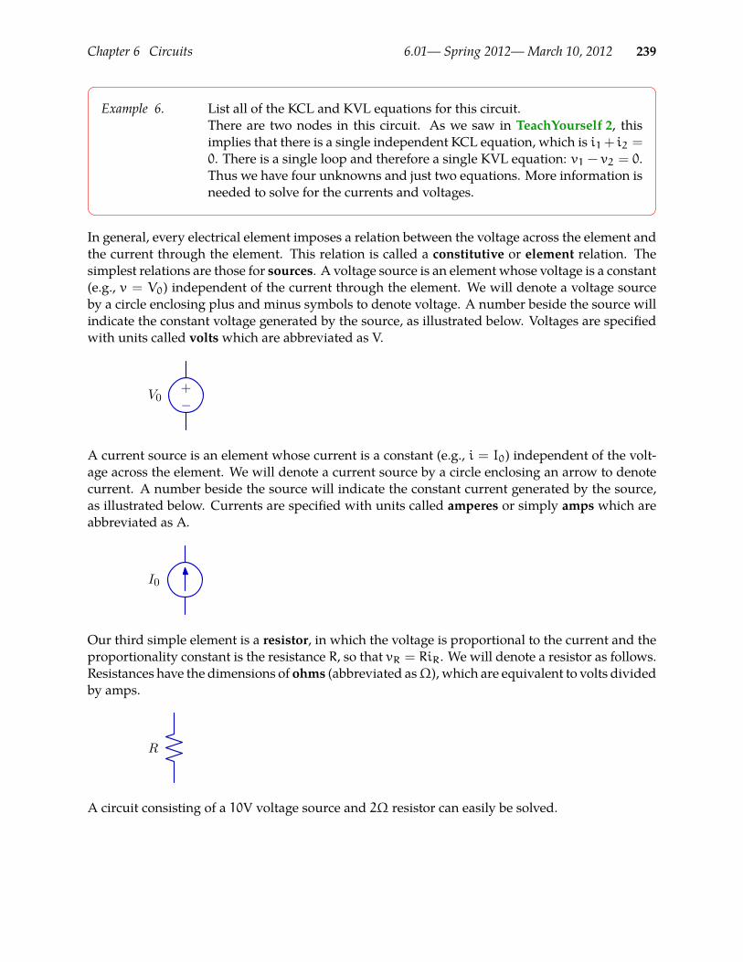
Chapter 6 Circuits 6.01— Spring 2012—March 10, 2012 239
Example 6. List all of the KCL and KVL equations for this circuit.There are two nodes in this circuit. As we saw in TeachYourself 2, thisimplies that there is a single independent KCL equation, which is i1+ i2 =0. There is a single loop and therefore a single KVL equation: v1 − v2 = 0.Thus we have four unknowns and just two equations. More information isneeded to solve for the currents and voltages.
In general, every electrical element imposes a relation between the voltage across the element andthe current through the element. This relation is called a constitutive or element relation. Thesimplest relations are those for sources. A voltage source is an element whose voltage is a constant(e.g., v = V0) independent of the current through the element. We will denote a voltage sourceby a circle enclosing plus and minus symbols to denote voltage. A number beside the source willindicate the constant voltage generated by the source, as illustrated below. Voltages are specifiedwith units called voltswhich are abbreviated as V.
+−
V0
A current source is an element whose current is a constant (e.g., i = I0) independent of the volt-age across the element. We will denote a current source by a circle enclosing an arrow to denotecurrent. A number beside the source will indicate the constant current generated by the source,as illustrated below. Currents are specified with units called amperes or simply amps which areabbreviated as A.
I0
Our third simple element is a resistor, in which the voltage is proportional to the current and theproportionality constant is the resistance R, so that vR = RiR. We will denote a resistor as follows.Resistances have the dimensions of ohms (abbreviated asΩ), which are equivalent to volts dividedby amps.
R
A circuit consisting of a 10V voltage source and 2Ω resistor can easily be solved.
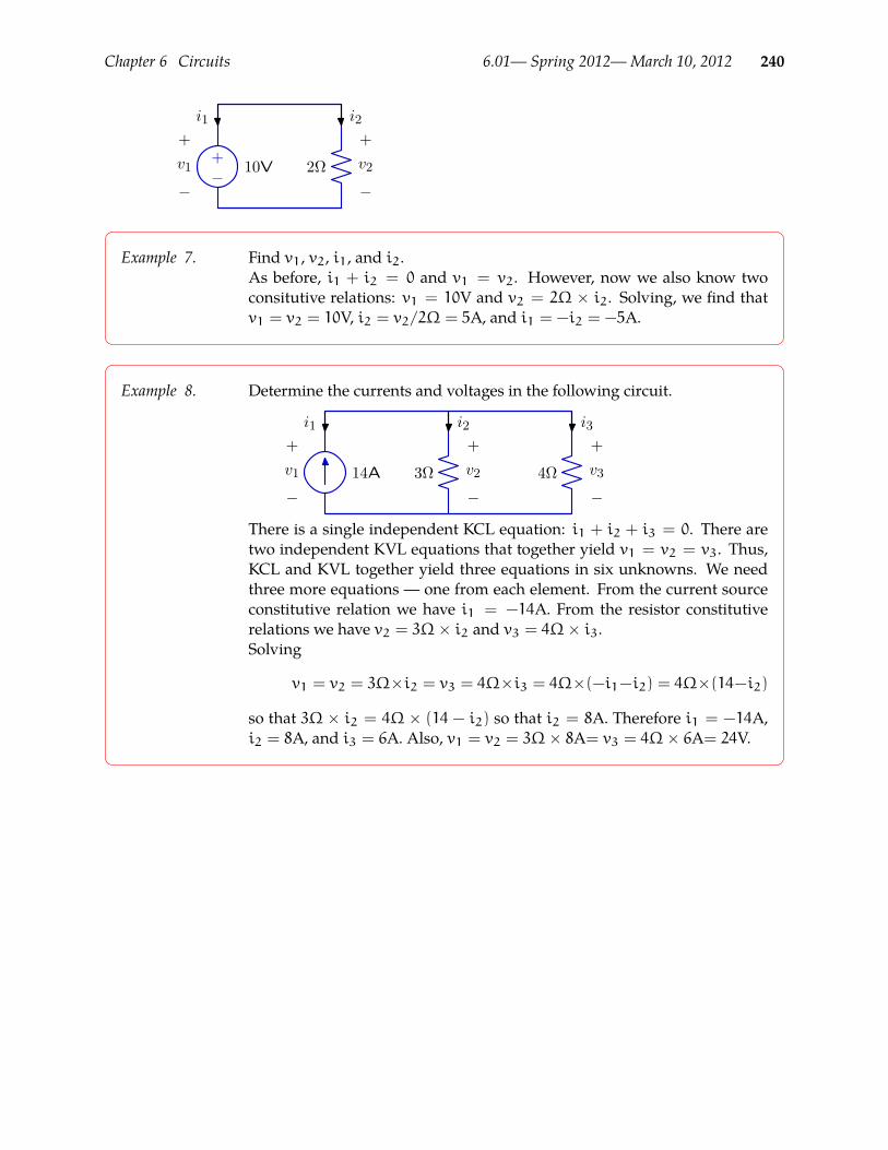
Chapter 6 Circuits 6.01— Spring 2012—March 10, 2012 240
+−
10V 2Ω
i1 i2+
−
v1
+
−
v2
Example 7. Find v1, v2, i1, and i2.As before, i1 + i2 = 0 and v1 = v2. However, now we also know twoconsitutive relations: v1 = 10V and v2 = 2Ω × i2. Solving, we find thatv1 = v2 = 10V, i2 = v2/2Ω = 5A, and i1 = −i2 = −5A.
Example 8. Determine the currents and voltages in the following circuit.
14A 3Ω 4Ω
i1 i2 i3+
−
v1
+
−
v2
+
−
v3
There is a single independent KCL equation: i1 + i2 + i3 = 0. There aretwo independent KVL equations that together yield v1 = v2 = v3. Thus,KCL and KVL together yield three equations in six unknowns. We needthree more equations — one from each element. From the current sourceconstitutive relation we have i1 = −14A. From the resistor constitutiverelations we have v2 = 3Ω× i2 and v3 = 4Ω× i3.Solving
v1 = v2 = 3Ω×i2 = v3 = 4Ω×i3 = 4Ω×(−i1−i2) = 4Ω×(14−i2)
so that 3Ω × i2 = 4Ω × (14 − i2) so that i2 = 8A. Therefore i1 = −14A,i2 = 8A, and i3 = 6A. Also, v1 = v2 = 3Ω× 8A= v3 = 4Ω× 6A= 24V.

Chapter 6 Circuits 6.01— Spring 2012—March 10, 2012 241
Example 9. Solve the following circuit.
+−
36V 3Ω 2Ω
6Ωi1
i2
i3 i4+
−
v1
+
−
v3
+
−
v4
+ −v2
Answer:
i1 = −5A ; i2 = 5A ; i3 = 2A ; i4 = 3A ;
v1 = 36V ; v2 = 30V ; v3 = 6V ; v4 = 6V
6.4 Solving circuitsGiven a description of the circuit’s wiring and a specification of the individual components, wecan solve the circuit to answer questions about particular voltages or currents in the circuit. Thereare several ways to approach this problem: wewill start with a completely systematic method thatis particularly useful if we want to solve circuits using a computer; then, we’ll see some simplermethod and patterns that are easier for humans to use.
The most obvious strategy would be to write down all the KVL and KCL equations, add the con-stituent equations for each element, and then solve for the voltage and current at each component.But we have a problem with redundant KVL equations. The voltages across circuit elements areconstrained by KVL so that the sum of the voltages around any closed loop is zero. However, thereare many possible closed loops through even simple circuits (see section 6.2.2). If we are dealingwith a planar circuit,41 then we know that all loops can be written as combinations of primitiveloops with non-overlapping interiors (see example 5).
Teach Yourself 5. Each of four nodes are connected to each of the others by a 1Ω resistor.How many resistors are there? Is the network planar?
Teach Yourself 6. Each of five nodes are connected to each of the others by a 1Ω resistor. Howmany resistors are there? Is the network planar?
So far, the only general way that we have seen to deal with this redundancy is to (1) find all of thepossible KVL equations, and then (2) eliminate the redundant ones. This process seems needlesslycomplicated.
A circuit is “planar” if it is possible to draw all of the elements and all of the lines that connect the elements without any41
of the lines or elements crossing over one another.

Chapter 6 Circuits 6.01— Spring 2012—March 10, 2012 242
One good way to eliminate KVL redundancy is to use node voltages. Node voltages are voltagesassociated with circuit nodes rather than with circuit elements. Given a complete set of node volt-ages, it is easy to determine the element voltages: each element voltage is the difference betweenthe voltage of the node at the positive end of the element minus that at its negative end.
Example 10. Determine expressions for each of the element voltages from the node volt-ages e0, e1, e2, and e3.
+−
V0
+
−
v1
+
−v2
+
−v3
+
−v4
+
−v5
+ −v6e1 e2
e0
e3
Answers: v1 = e3 − e0; v2 = e3 − e1; v3 = e3 − e2; v4 = e1 − e0; v5 = e2 − e0; v6 = e1 − e2;
Example 11. Howwould the element voltages in the previous example change if 1Vwereadded to each of the node voltages?
Adding a constant voltage to each of the node voltages of a circuit has no effect on any of theelement voltages. Thus, substituting node voltages for element voltages removes redundanciesthat are implicit in KCL equations, but also introduces a new redundancy, which we can think ofas a global offset voltage. If we are only interested in element voltages (which is typically the case),we can exclude effects of a global offset voltage by arbitrarily assigning the potential of one nodeto zero. We refer to that special node with zero potential as the “ground.”
We will explore two methods that use node voltages: the node-voltage-and-component-current(NVCC) method, which has variables for voltages at all of the nodes and currents through all ofthe components, and the node method, which only has variables for voltages at the nodes. TheNVCCmethod is completely general, but rather long-winded (and is perhaps better for computersto use than humans). The node method is terser, with potentially many fewer equations, but canbecome complicated when there are multiple voltage sources.
6.4.1 NVCCMethodIn the NVCC method, we take the following steps:1. Label all of the nodes (places where there is a wire between two or more components) with
names n1, . . . , nn, and make variables v1, . . . , vn, one for the voltage at each node.2. Declare one of them, ng, to be the ground node (this can be any node; the voltages will be
computed relative to the voltage at that node) and set vg = 0.

Chapter 6 Circuits 6.01— Spring 2012—March 10, 2012 243
3. Make current variables i1, . . . , im for each component (resistor or source) in the network. Labela direction for each current in your network (it doesn’t matter what directions you pick as longas you handle them consistently from here on out).
4. Write down n− 1 KCL equations, one for each node except for ng. These equations assert thatthe sum of currents entering each node is 0.
5. Write down m constitutive equations, one for each component, describing that component’slinear relationship between its current ik and the voltage difference across the component.The voltage across the component is vk+ − vk−, where vk+ is the node voltage at the positiveterminal of the component and vk− is the node voltage at its negative terminal voltage. Thedirection of the current defines what constitutes the ’positive’ and ’negative’ terminals of thecomponent: the current runs from positive to negative.
For a resistor with resistance R, the equation is vk+ − vk− = ikR; for a voltage source withvoltage Vs, the equation is vk+ − vk− = Vs; for a current source with current Cs, the equationis ik = Cs.
6. Solve these equations to determine the node voltage and component currents.
So, for this circuit,
Vc
n2
n3
n1 iA
iB
iC
iD
RA
RB
RD
using the current directions for each component as drawn, we have the following equations:• Ground
v3 = 0 .
• KCL
iA − iB − iD − iC = 0
iB − iA = 0 .
• Constitutive equations
(v1 − v2) = iA · RA(v2 − v1) = iB · RB(v2 − v3) = iD · RDv2 − v3 = Vc .

Chapter 6 Circuits 6.01— Spring 2012—March 10, 2012 244
So, now, if we know RA, RB, RD, and VC, which are the specifications of our components, we have7 linear equations in 7 unknowns (v1, v2, v3, iA, iB, iC, and iD). Just a small (though possiblytedious) matter of algebra, and we’re done.
As an example, let RA = 100Ω, RB = 200Ω, RD = 100Ω, and VC = 10V . Then, we get v2 = 10V ;iA = iB = 0A (that’s reasonable: why would any current bother going that way, when it can justrun through the diagonal wire?); and iD = 0.1A, which is pretty straightforward.
6.4.2 Solution strategyYou can see that the KCL equations are all in terms of currents; and the constitutive equationsgive us direct expressions for almost all of the currents. So, a good solution strategy is to workprimarily with the KCL equations, trying to eliminate as many current variables as possible, bysubstituting in expressions derived from the constitutive equations. In the example above, hereare the KCL equations:
iA − iB − iD − iC = 0
iB − iA = 0 .
Now, substituting in expressions from the constitutive equations, we can rewrite them as:v1 − v2RA
−v2 − v1RB
−Vc
RD− iC = 0
v2 − v1RB
−v1 − v2RA
= 0 .
We also know, from the ground equation v3 = 0, that v2 = VC, so we can rewrite our equationsas:
v1 − VcRA
−Vc − v1RB
−Vc
RD− iC = 0
Vc − v1RB
−v1 − VcRA
= 0 .
In most cases, you can write equations of this form down directly, without bothering to writethe KCL and the constituent equations separately, and then substituting in for the currents.
Now we only have two unknowns: v1 and iC, and two equations. The second equation tells usthat Vc = V1, and, substituting that into the first equation, we have
iC =Vc
RD
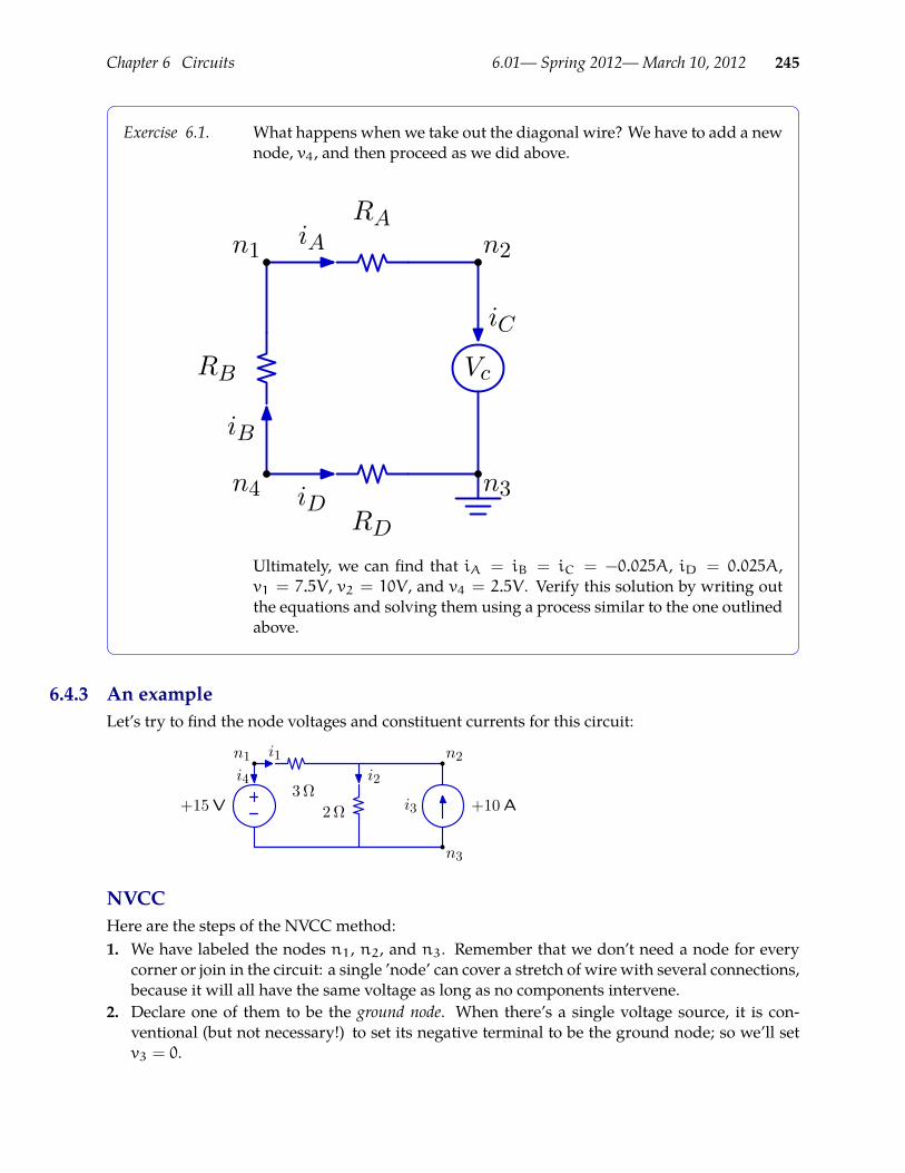
Chapter 6 Circuits 6.01— Spring 2012—March 10, 2012 245
Exercise 6.1. What happens when we take out the diagonal wire? We have to add a newnode, v4, and then proceed as we did above.
Vc
n2
n3n4
n1 iA
iB
iC
iD
RA
RB
RD
Ultimately, we can find that iA = iB = iC = −0.025A, iD = 0.025A,v1 = 7.5V , v2 = 10V , and v4 = 2.5V . Verify this solution by writing outthe equations and solving them using a process similar to the one outlinedabove.
6.4.3 An exampleLet’s try to find the node voltages and constituent currents for this circuit:
+10 A+15 V3 Ω
2 Ω
n1 n2
n3
i1i2
i3
i4
NVCCHere are the steps of the NVCC method:1. We have labeled the nodes n1, n2, and n3. Remember that we don’t need a node for every
corner or join in the circuit: a single ’node’ can cover a stretch of wire with several connections,because it will all have the same voltage as long as no components intervene.
2. Declare one of them to be the ground node. When there’s a single voltage source, it is con-ventional (but not necessary!) to set its negative terminal to be the ground node; so we’ll setv3 = 0.

Chapter 6 Circuits 6.01— Spring 2012—March 10, 2012 246
3. Make current variables for each component in the network and label them with arrows. Wedid this already in the figure.
4. Write down n− 1 KCL equations, one for each node except for the ground node.
− i4 − i1 = 0
i1 − i2 + i3 = 0
5. Write down m constitutive equations, one for each component, describing that component’slinear relationship between its current ik and the voltage difference across the component.
v1 = 15
v1 − v2 = 3i1
v2 − v3 = 2i2
i3 = 10
6. Solve these equations to determine the node voltage and component currents. There are lotsof ways to work through this algebra. Here’s one meandering path to the right answer.
We can do some plugging in of v1, v3, and i3 to simplify matters.
15− v2 = 3i1
v2 = 2i2
− i4 − i1 = 0
i1 − i2 + 10 = 0
Plugging expressions for i1 and i2 derived from the first two equations into the last one, weget
15− v23
−v2
2= −10
so
v2 = 18
And now it’s easy to see that i1 = −1, i2 = 9, and i4 = 1.
NVCC ShortcutIf we want to shortcut the NVCC method, we can follow the first three steps above, but then tryto go straight to versions of the KCL equations that substitute in expressions for current that arederived from the constituent constraints. So, we could observe that if v3 = 0 then v1 = 15. Andthen we could write the KCL equations as:
− i4 −15− v23
= 0
15− v23
+ 10−v2
2= 0
Solving the second equation we find that v2 = 18; from this we can easily determine the otherrelevant quantities.

Chapter 6 Circuits 6.01— Spring 2012—March 10, 2012 247
6.4.4 Node method (optional)Node analysis is similar to NVCC, but with the goal of writing down one equation per node.
We can further simplify the node representation of circuits that contain voltage sources. When avoltage source connects two nodes, it constrains the two node voltages so that one can be deter-mined from the other, as shown in the following figure, where e0 in the previous figure is takenas ground.
+−
V0
+
−
v1
+
−v2
+
−v3
+
−v4
+
−v5
+ −v6e1 e2
gnd
V0
So far, we have seen that node voltages are a concise representation of all of the information that isnecessary to compute the element voltages of a circuit. Furthermore, node voltages automaticallyguarantee that KVL is satisfied by all of the element voltages. To complete the analysis of a circuitusing node voltages, we must next consider the element currents and KCL.
In general, one can write KCL at each of the nodes of a circuit. However, as we saw inTeachYourself 2, one of those equations will always be linearly dependent on the others. Thus, ifthe circuit has n nodes, we can write n− 1 independent KCL equations.
If there are no voltage sources in the circuit, then we can express each KCL equation as a sumof element currents that can each be determined from the node voltages by using the element’sconstitutive equation. The result is a system of n−1KCL equations that can be expressed in termsof n− 1 node voltage variables.
If there are voltage sources in the circuit, then two additional issues arise. First, each voltage sourceconnects two nodes, but is represented by just one node variable (since the voltage of the sourcedetermines the voltage at the other node). Second, the current through a voltage source cannotbe determined from its constitutive equation. The constitutive equation for a voltage source isvs = V0, whichmust be true for all currents. Thus, knowing that vs = V0 provides no informationabout the current through the source. These constraints are illustrated below.
+−
V0
i1i2
i3
i4i5
i6
ek
ek + V0

Chapter 6 Circuits 6.01— Spring 2012—March 10, 2012 248
A consistent set of equations can be derived by treating the entire voltage source as a single node,represented by the dashed green box above. The KCL equation for that node,
i1 + i2 + i3 + i4 + i5 + i6 = 0
involves element currents that can each be written (using their constitutive equations) in terms ofnode voltages outside the box plus ek and ek + V0. Like the KCL equations outside the box, thisKCL equation adds a single new unknown, which is ek.
Example 12. Does the above analysis imply that the current through the voltage sourceis zero?
No. Let iv represent the current through the voltage source. KCL at the top node requires that
i1 + i2 + i3 + iv = 0
KCL at the bottom node requires that
i4 + i5 + i6 − iv = 0
The sum of these equations is the KCL equation given above for the dashed green box. It holdsreguardless of the value of the current through the voltage source. To find the value of the currentthrough the current source, first solve for i1, i2, i3, i4, i5, i6, and ek, ignoring iv. Then iv =−(i1 + i2 + i3), which will be the same as i4 + i5 + i6.
Teach Yourself 7. How would you handle a circuit in which i1 (above) connects directly toanother voltage source outside the dashed green box?
Node Analysis: Summary• Assign a voltage expression to each node in the circuit, as follows:
− Assign a voltage of zero to one node, which is called the “ground.”− Assign voltages to nodes that are connected to voltage sources so that the voltage
source relations are satisfied:? If the voltage on one terminal of a voltage source is known (e.g., ground), then use
the voltage source relation to determine the node voltage on the other terminal.? If neither terminal of the voltage source connects to a known voltage, then assign
a variable to represent the node voltage at one terminal and use the voltage sourcerelation to determine the node voltage at the other terminal.
− Assign variables to represent the voltages at all remaining nodes.• For each element in the circuit that is not a voltage source, use the associated constitu-
tive law to express the current through the element in terms of the node voltages at itsterminals.
• Write one KCL equation for each unknown node voltage, as follows:− Express KCL for each node that is not connected to a voltage source as a sumof element
currents.− For each voltage source, write a single KCL to express the sum of currents entering the
nodes connected to both its positive and negative terminals.
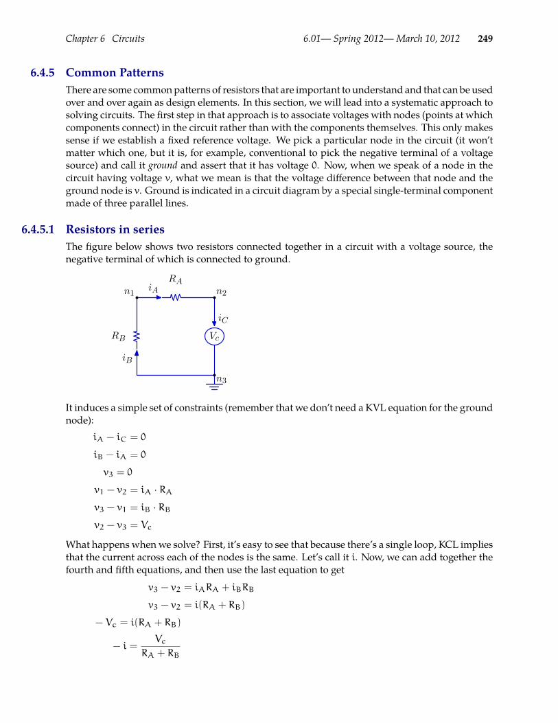
Chapter 6 Circuits 6.01— Spring 2012—March 10, 2012 249
6.4.5 Common PatternsThere are some commonpatterns of resistors that are important to understand and that can be usedover and over again as design elements. In this section, we will lead into a systematic approach tosolving circuits. The first step in that approach is to associate voltages with nodes (points at whichcomponents connect) in the circuit rather than with the components themselves. This only makessense if we establish a fixed reference voltage. We pick a particular node in the circuit (it won’tmatter which one, but it is, for example, conventional to pick the negative terminal of a voltagesource) and call it ground and assert that it has voltage 0. Now, when we speak of a node in thecircuit having voltage v, what we mean is that the voltage difference between that node and theground node is v. Ground is indicated in a circuit diagram by a special single-terminal componentmade of three parallel lines.
6.4.5.1 Resistors in seriesThe figure below shows two resistors connected together in a circuit with a voltage source, thenegative terminal of which is connected to ground.
Vc
n2
n3
n1RA
RB
iA
iB
iC
It induces a simple set of constraints (remember that we don’t need a KVL equation for the groundnode):
iA − iC = 0
iB − iA = 0
v3 = 0
v1 − v2 = iA · RAv3 − v1 = iB · RBv2 − v3 = Vc
What happens whenwe solve? First, it’s easy to see that because there’s a single loop, KCL impliesthat the current across each of the nodes is the same. Let’s call it i. Now, we can add together thefourth and fifth equations, and then use the last equation to get
v3 − v2 = iARA + iBRB
v3 − v2 = i(RA + RB)
− Vc = i(RA + RB)
− i =Vc
RA + RB
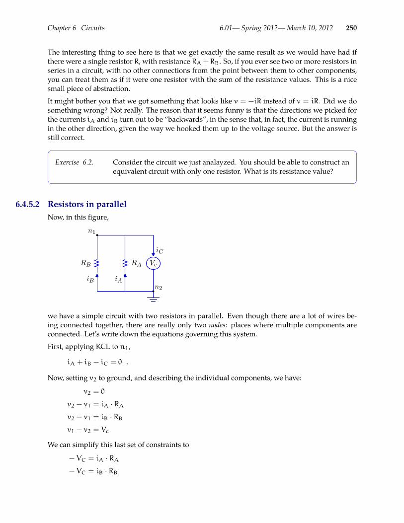
Chapter 6 Circuits 6.01— Spring 2012—March 10, 2012 250
The interesting thing to see here is that we get exactly the same result as we would have had ifthere were a single resistor R, with resistance RA+RB. So, if you ever see two or more resistors inseries in a circuit, with no other connections from the point between them to other components,you can treat them as if it were one resistor with the sum of the resistance values. This is a nicesmall piece of abstraction.
It might bother you that we got something that looks like v = −iR instead of v = iR. Did we dosomething wrong? Not really. The reason that it seems funny is that the directions we picked forthe currents iA and iB turn out to be “backwards”, in the sense that, in fact, the current is runningin the other direction, given the way we hooked them up to the voltage source. But the answer isstill correct.
Exercise 6.2. Consider the circuit we just analayzed. You should be able to construct anequivalent circuit with only one resistor. What is its resistance value?
6.4.5.2 Resistors in parallelNow, in this figure,
Vc
n2
n1
RARB
iAiB
iC
we have a simple circuit with two resistors in parallel. Even though there are a lot of wires be-ing connected together, there are really only two nodes: places where multiple components areconnected. Let’s write down the equations governing this system.
First, applying KCL to n1,
iA + iB − iC = 0 .
Now, setting v2 to ground, and describing the individual components, we have:
v2 = 0
v2 − v1 = iA · RAv2 − v1 = iB · RBv1 − v2 = Vc
We can simplify this last set of constraints to
− VC = iA · RA− VC = iB · RB

Chapter 6 Circuits 6.01— Spring 2012—March 10, 2012 251
so
iA = −Vc
RA
iB = −Vc
RB
Plugging these into the KCL equation, we get:
iA + iB − iC = 0
−Vc
RA−Vc
RB= iC
− VcRA + RBRARB
= iC
− Vc = iCRARB
RA + RB
What we can see from this is that two resistances, RA and RB, wired up in parallel, act like a singleresistor with resistance
RARB
RA + RB.
This is another common pattern for both analysis and design. If you see a circuit with parallelresistors connected at nodes n1 and n2, you can simplify it to a circuit that replaces those twopaths between n1 and n2 with a single path with a single resistor.
To get some intuition, think about what happens when RA is much bigger than RB. Because thevoltage across both resistors is the same, it must be that the current through RA is much smallerthan the current through RB. The appropriate intuition here is that current goes through theresistor that’s easier to pass through.
Exercise 6.3. If RA = 10000Ω and RB = 10Ω, what is the effective resistance of RA andRB in parallel?
6.4.5.3 Voltage dividerThe figure below shows part of a circuit, in a configuration known as a voltage divider.
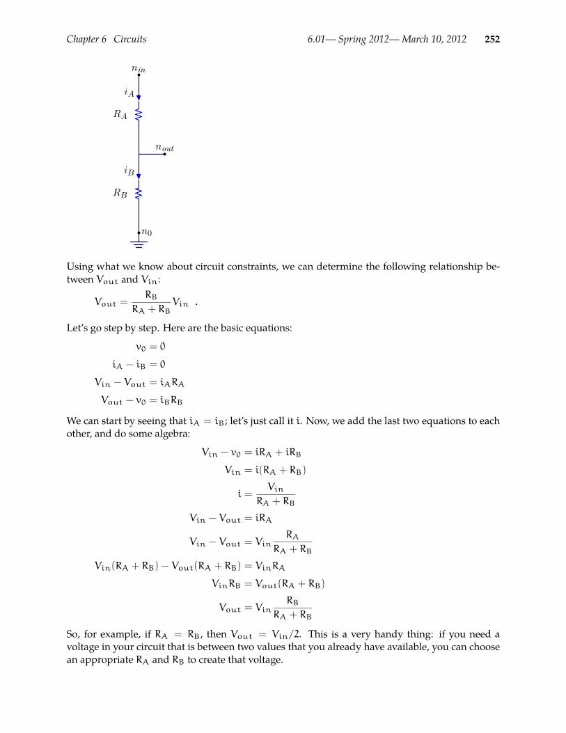
Chapter 6 Circuits 6.01— Spring 2012—March 10, 2012 252
nin
nout
n0
RB
RA
iA
iB
Using what we know about circuit constraints, we can determine the following relationship be-tween Vout and Vin:
Vout =RB
RA + RBVin .
Let’s go step by step. Here are the basic equations:
v0 = 0
iA − iB = 0
Vin − Vout = iARA
Vout − v0 = iBRB
We can start by seeing that iA = iB; let’s just call it i. Now, we add the last two equations to eachother, and do some algebra:
Vin − v0 = iRA + iRB
Vin = i(RA + RB)
i =Vin
RA + RB
Vin − Vout = iRA
Vin − Vout = VinRA
RA + RB
Vin(RA + RB) − Vout(RA + RB) = VinRA
VinRB = Vout(RA + RB)
Vout = VinRB
RA + RB
So, for example, if RA = RB, then Vout = Vin/2. This is a very handy thing: if you need avoltage in your circuit that is between two values that you already have available, you can choosean appropriate RA and RB to create that voltage.
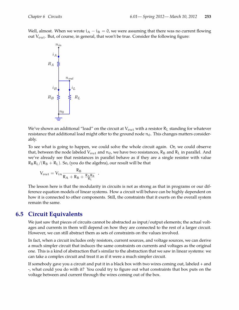
Chapter 6 Circuits 6.01— Spring 2012—March 10, 2012 253
Well, almost. When we wrote iA − iB = 0, we were assuming that there was no current flowingout Vout. But, of course, in general, that won’t be true. Consider the following figure:
nin
nout
n0
RB
RA
RL
iA
iB iL
We’ve shown an additional “load” on the circuit at Vout with a resistor RL standing for whateverresistance that additional load might offer to the ground node n0. This changes matters consider-ably.
To see what is going to happen, we could solve the whole circuit again. Or, we could observethat, between the node labeled Vout and n0, we have two resistances, RB and RL in parallel. Andwe’ve already see that resistances in parallel behave as if they are a single resistor with valueRBRL/(RB + RL). So, (you do the algebra), our result will be that
Vout = VinRB
RA + RB + RARBRL
.
The lesson here is that the modularity in circuits is not as strong as that in programs or our dif-ference equation models of linear systems. How a circuit will behave can be highly dependent onhow it is connected to other components. Still, the constraints that it exerts on the overall systemremain the same.
6.5 Circuit EquivalentsWe just saw that pieces of circuits cannot be abstracted as input/output elements; the actual volt-ages and currents in them will depend on how they are connected to the rest of a larger circuit.However, we can still abstract them as sets of constraints on the values involved.
In fact, when a circuit includes only resistors, current sources, and voltage sources, we can derivea much simpler circuit that induces the same constraints on currents and voltages as the originalone. This is a kind of abstraction that’s similar to the abstraction that we saw in linear systems: wecan take a complex circuit and treat it as if it were a much simpler circuit.
If somebody gave you a circuit and put it in a black box with two wires coming out, labeled + and-, what could you do with it? You could try to figure out what constraints that box puts on thevoltage between and current through the wires coming out of the box.

Chapter 6 Circuits 6.01— Spring 2012—March 10, 2012 254
We can start by figuring out the open-circuit voltage across the two terminals. That is the voltagedropwe’d see across the twowires if nothingwere connected to them. We’ll call thatVoc. Anotherthingwe could do is connect the twowires together, and see howmuch current runs through them;this is called the short-circuit current. We’ll call that isc.
Because all of the relationships in our circuits are linear, these two values are sufficient to charac-terize the constraint that this whole box will exert on a circuit connected to it. The constraint willbe a relationship between the voltage across its terminals and the current flowing through the box.We can derive it by using Thévenin’s theorem:
Any combination of current sources, voltage sources, and resistances with two terminals canbe replaced by a single voltage source Vth and a single series resistor Rth. The value of Vthis the open circuit voltage at the terminals Voc, and the value of Rth is Vth divided by thecurrent with the terminals short circuited (−isc).
Let’s look at a picture, then an example.
+
-VTH
iTH
RTH n+
n-
i
Here, we show a picture of a black (well, gray) box, abstracted as being made up of a circuit witha single voltage source Vth and a single resistor Rth in series. The open-circuit voltage from n+
to n− is clearly Vth. The short-circuit current isc (in the direction of the arrow) is −Vth/Rth. So,this circuit would have the desired measured properties.42
Now, here is an actual circuit. We’ll compute its associated open-circuit voltage and short-circuitcurrent, construct the associated Thévenin equivalent circuit, and be sure it has the same properties.
The minus sign here can be kind of confusing. The issue is this: when we are treating this circuit as a black box with42
terminals n+ and n−, we think of the current flowing out of n+ and in to n−, which is consistent with the voltagedifference Vth = V+ − V−. But when we compute the short-circuit current by wiring n+ and n− together, we arecontinuing to think of isc as flowing out of n+, but now it is coming out of n− and in to n+, which is the oppositedirection. So, we have to change its sign to compute Rth.
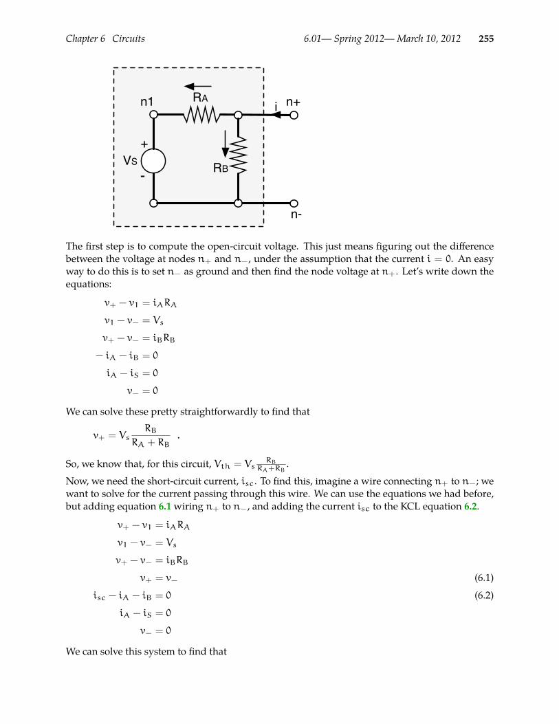
Chapter 6 Circuits 6.01— Spring 2012—March 10, 2012 255
+
-VS
RA n+
n-
i
RB
n1
The first step is to compute the open-circuit voltage. This just means figuring out the differencebetween the voltage at nodes n+ and n−, under the assumption that the current i = 0. An easyway to do this is to set n− as ground and then find the node voltage at n+. Let’s write down theequations:
v+ − v1 = iARA
v1 − v− = Vs
v+ − v− = iBRB
− iA − iB = 0
iA − iS = 0
v− = 0
We can solve these pretty straightforwardly to find that
v+ = VsRB
RA + RB.
So, we know that, for this circuit, Vth = VsRB
RA+RB.
Now, we need the short-circuit current, isc. To find this, imagine a wire connecting n+ to n−; wewant to solve for the current passing through this wire. We can use the equations we had before,but adding equation 6.1wiring n+ to n−, and adding the current isc to the KCL equation 6.2.
v+ − v1 = iARA
v1 − v− = Vs
v+ − v− = iBRB
v+ = v− (6.1)
isc − iA − iB = 0 (6.2)
iA − iS = 0
v− = 0
We can solve this system to find that
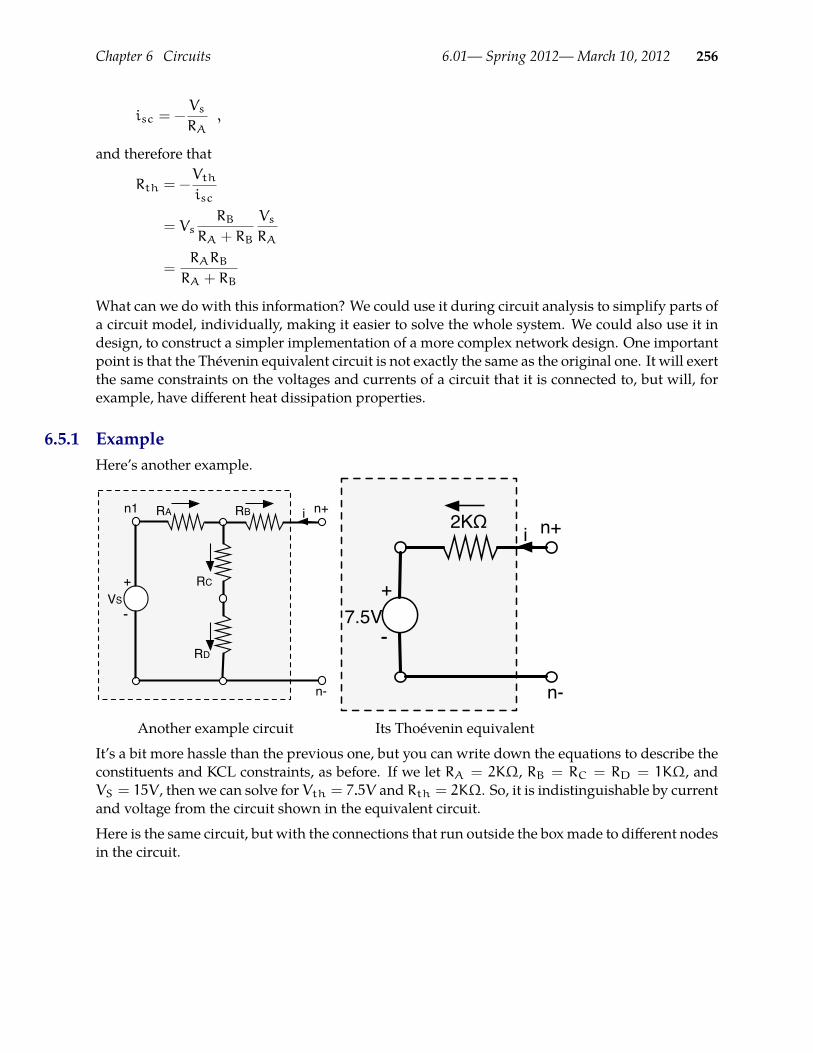
Chapter 6 Circuits 6.01— Spring 2012—March 10, 2012 256
isc = −Vs
RA,
and therefore that
Rth = −Vth
isc
= VsRB
RA + RB
Vs
RA
=RARB
RA + RB
What can we do with this information? We could use it during circuit analysis to simplify parts ofa circuit model, individually, making it easier to solve the whole system. We could also use it indesign, to construct a simpler implementation of a more complex network design. One importantpoint is that the Thévenin equivalent circuit is not exactly the same as the original one. It will exertthe same constraints on the voltages and currents of a circuit that it is connected to, but will, forexample, have different heat dissipation properties.
6.5.1 ExampleHere’s another example.
+
-VS
RA n+
n-
i
RC
n1
RD
RB
+
-7.5V
2KΩ n+
n-
i
Another example circuit Its Thoévenin equivalent
It’s a bit more hassle than the previous one, but you can write down the equations to describe theconstituents and KCL constraints, as before. If we let RA = 2KΩ, RB = RC = RD = 1KΩ, andVS = 15V , then we can solve for Vth = 7.5V and Rth = 2KΩ. So, it is indistinguishable by currentand voltage from the circuit shown in the equivalent circuit.
Here is the same circuit, but with the connections that run outside the boxmade to different nodesin the circuit.

Chapter 6 Circuits 6.01— Spring 2012—March 10, 2012 257
+
-VS
RA
n+
n-
iRC
n1
RD
RB
+
-3.75V
1750Ω n+
n-
i
Same circuit, different ports Its Thévenin equivalent
Note also that the top lead ismarkedn− and the bottom onen+. If we solve, using the same valuesfor the resistors and voltage source as before, we find that Vth = −3.75V and Rth = 1750Ω. Weshow the Thévenin equivalent circuit next to the original. We’ve changed the polarity of the voltagesource and made it 3.75V (instead of having the + terminal at the top and a voltage of -3.75), butthat’s just a matter of drawing.
These results are quite different: so, the moral is, it matters which wires you connect up to what!
6.5.2 Norton EquivalentsIt is also possible to derive an equivalent circuit consisting of a single resistor in parallel with asingle current source. Such a circuit is called a Norton equivalent circuit. The process for derivingNorton equivalents is similar in spirit to the process outlined above.
6.6 Op AmpsSo far, we have considered circuits with resistors, voltage sources, and current sources. Now weare going introduce a new component, called an operational amplifier or op-amp, for short. Op-ampsare a crucial tool for decoupling some aspects of complex circuits, so that they can be designed in-dependently and then connected. They are also important for amplifying small voltage differencesinto larger ones, and can be used to scale, invert, and add voltages.
6.6.1 Voltage-controlled voltage sourcesIn fact, op-amps are complex assemblages of transistors and other circuit components. We’ll needa simpler model than that of what they do, so that we can analyze circuits that contain them, anddesign new circuits that use them.
We will think about an op-amp as a voltage-controlled voltage source (VCVS). Op-amps have fourterminals, two of which are often called the input terminals and two, the output terminals. Wecan think of the op-amp as a voltage source, in which the voltage difference across the outputterminals is controlled by the voltage difference between the input terminals. The crucial thingabout a voltage source is that it maintains the voltage difference that it is trying to source, nomatter what it is connected to.

Chapter 6 Circuits 6.01— Spring 2012—March 10, 2012 258
n-
n+ nout
K(v+! v!)
ngnd
i
Amodel of the constraint that an op-amp exerts on the circuit it is connected to relates the voltagesat its four terminals in this way:
vout − vgnd = K(v+ − v−) ,
where K is a very large gain, on the order of 10,000, and asserts that no current flows into the opamp.
i+ = i− = 0 .
So, we can think of nout and ngnd as constituting a voltage source, whose voltage is defined to beK(v+−v−). We can see it as amplifying the voltage difference v+−v−. It’s hard to really understandhow this model works without seeing it in context. So, we’ll study an op-amp that is wired up ina configuration called a voltage follower:
n-
n+ nout
+
-VC
K(v+! v!)
i
Note that we have connected a wire from the output, nout, to the negative input, n−, and so thoseconstitute one node with a single voltage, which we call vout. We can write down the equations:
v+ = Vc
vout − vgnd = K(v+ − vout)
vgnd = 0
Solving this system, we find that
vout = VcK
K+ 1.
So, for large K, the voltage difference between the output terminals is very close to the voltagedifference between the input terminals.
In this circuit we have set vgnd = 0; in practice this doesn’t matter. If we had left vgnd in ourequations, we would have found that:
vout = VcK
K+ 1+ vgnd
1
K+ 1.

Chapter 6 Circuits 6.01— Spring 2012—March 10, 2012 259
Since K is very large, that second term can be ignored. In fact, if you look at an actual op-amp, youwon’t even find an output corresponding to ngnd. Therefore, we will always treat it as being zero.
The crucial additional fact about an op-amp is that no current flows between the input and outputterminals, so the op-amp acts as a buffer between the input and output signal. It provides a discon-nect between the currents on either side of it. This is a big deal: it gives us a kind of modularity inour circuits that we haven’t had before, by limiting the kinds of influence of one part of the circuiton the other. The ability to partially disconnect sub-parts of our circuits will make it easier to docomplex designs.
We can appreciate the value of a buffer in the context of using a variable voltage to control a motor.If we have a 15V supply, but only want to put 7.5V across the motor terminals, what should wedo? A voltage divider seems like a good strategy: we can use one with two equal resistances, tomake 7.5V , and then connect it to the motor as shown here
nmotor
10K
+15V
RmotorMotor10K
But what will the voltage vmotor end up being? It all depends on the resistance of the motor. If themotor is offering little resistance, say 100Ω, then the voltage vmotor will be very close to 0.43 So, thisis not an effective solution to the problem of supplying 7.5V to the motor.
So, now, back to the motor. In this figure,
Go back and review the discussion of adding a load to a voltage divider, if this doesn’t seem clear.43

Chapter 6 Circuits 6.01— Spring 2012—March 10, 2012 260
n-
n+ nout
Rmotor
Motor
10K
+15V
10K
K(v+! v!)
i
we have used a voltage follower to connect the voltage divider to themotor. Based on our previousanalysis of the follower, we expect the voltage at nout to be 7.5V , at least before we connect it upto the motor. Let’s see how this all works out by writing the equations out for the whole circuit:Letting the current through the top resistor be i1, the current through the second resistor be i2,the current through the motor be im, and recalling that vout = v− (since they are the same node),we have
i1 − i2 − i+ = 0
− iout − i− − im = 0
i+ = 0
i− = 0
(15− v+) = 10000i1
(v+ − 0) = 10000i2
(v− − 0) = K(v+ − v−)
(v− − 0) = imRm
Solving these equations, we find that
v+ = 7.5
v− =K
K+ 17.5
im =K
K+ 1
7.5
Rm
So, now, the voltage across the motor stays near 7.5V , and because of the isolation provided by theop-amp, it will remain that way, no matter what the resistance of the motor. Further, if in fact the

Chapter 6 Circuits 6.01— Spring 2012—March 10, 2012 261
motor has resistance of 5Ω, then we can find that the (maximum) current through the motor, im,is approximately 1.5A.
6.6.2 Simplified modelThe voltage-controlled voltage-source model allows us to use our standard linear-equation formof reasoning about circuit values, but it can become cumbersome to deal with the K’s all the time.In most of the usual applications of an op-amp, we will find that we can use a simpler model toreason about what is happening. That simpler model also comes with a simpler picture:
-
+
n-
n+nout
The simplified behavioral model is that the op-amp adjusts vout in order to try to maintain theconstraint that v+ ≈ v− and that no current flows in to n+ or n−. In what follows we will assumethat the op-amp enforces v+ = v−.
In this section, we will explore several standard applications of op-amps, using this simplifiedmodel. If it becomes confusing, you can always go back and apply the VCVS model from theprevious section.
Non-inverting amplifierNot surprisingly, a primary use of an op-amp is as an amplifier. Here is an amplifier configuration,like this.
-
+
n-
ninnout
RI
RF
Let’s see if we can figure out the relationship between vin and vout. The circuit constraints tell usthat

Chapter 6 Circuits 6.01— Spring 2012—March 10, 2012 262
v− = iIRI
v− − vout = iFRF
− iI − iF = 0 (6.3)
vin = v− (6.4)
The KCL equation (6.3) has no term for the current into the op-amp, because we assume it is zero.Equation 6.4 is the op-amp constraint. So, we find that
vout = vinRF + RIRI
.
This is cool. We’ve arranged for the output voltage to be greater than the input voltage. We canget any gain (greater than one) by choosing the values of RF and RI.We can think intuitively about how it works by examining some cases. First, if RF = 0, then we’llhave vout = vin, so there’s not a particularly interesting change in the voltages. This is still a usefuldevice, essentially the voltage follower, which we have already seen, with an additional resistor.This extra resistor does not change the voltage relationsips but does increase the current flowingfrom the op-amp. Note also that choosing RI very much larger than RF also gives us a follower.Now let’s think about a more interesting case, but simplify matters by setting RF = RI. We canlook at the part of the circuit running from Vout through RF and RI to ground. This looks a lot likea voltage divider, with v− coming out of the middle of it. Because v− needs to be the same as vin,and it is vout being divided in half, then vout clearly has to be 2vin.
Inverting amplifierHere is a very similar configuration, called an inverting amplifier.
-
+
n-
nin
nout
RI RF
n+
The difference is that the + terminal of the op-amp is connected to ground, and the we’re think-ing of the path through the resistors as the terminal of the resulting circuit. Let’s figure out therelationship between vin and vout for this one. The circuit constraints tell us that
vin − v− = iIRI
v− − vout = iFRF
iI − iF = 0
v+ = v−
v+ = 0
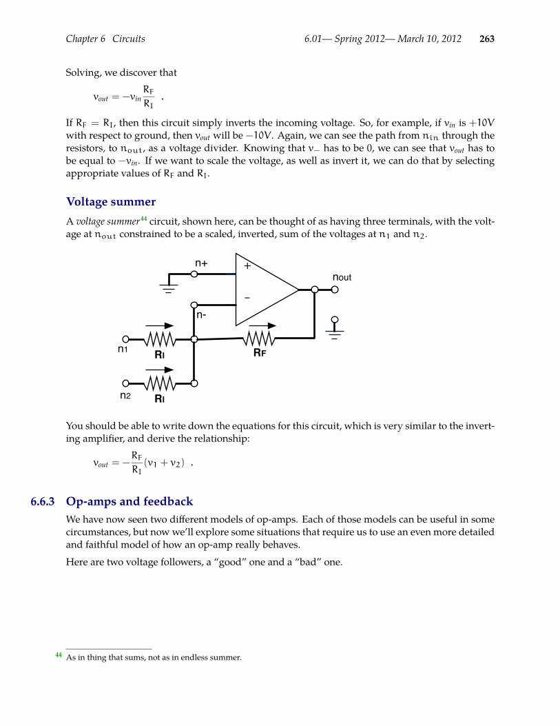
Chapter 6 Circuits 6.01— Spring 2012—March 10, 2012 263
Solving, we discover that
vout = −vinRF
RI.
If RF = RI, then this circuit simply inverts the incoming voltage. So, for example, if vin is +10Vwith respect to ground, then vout will be −10V . Again, we can see the path from nin through theresistors, to nout, as a voltage divider. Knowing that v− has to be 0, we can see that vout has tobe equal to −vin. If we want to scale the voltage, as well as invert it, we can do that by selectingappropriate values of RF and RI.
Voltage summerA voltage summer44 circuit, shown here, can be thought of as having three terminals, with the volt-age at nout constrained to be a scaled, inverted, sum of the voltages at n1 and n2.
-
+
n-
n1
nout
RI RF
n+
RIn2
You should be able to write down the equations for this circuit, which is very similar to the invert-ing amplifier, and derive the relationship:
vout = −RF
RI(v1 + v2) .
6.6.3 Op-amps and feedbackWe have now seen two different models of op-amps. Each of those models can be useful in somecircumstances, but nowwe’ll explore some situations that require us to use an even more detailedand faithful model of how an op-amp really behaves.
Here are two voltage followers, a “good” one and a “bad” one.
As in thing that sums, not as in endless summer.44

Chapter 6 Circuits 6.01— Spring 2012—March 10, 2012 264
-
+
n-
n+nout
+
-VC -
+
n-
n+nout
+
-VC
“Good” voltage follower “Bad” voltage follower
If we use our simplest model to predict their behavior, in both cases, we’ll predict that vout = Vc.If we use the VCVS model, we’ll predict that, for the good follower vout = Vc
KK+1 . For the bad
follower, things are connected a little bit differently:
v− = Vc
vout − vgnd = K(v+ − v−)
v+ = vout
vgnd = 0
Solving this system, we find that
vout = VcK
K− 1.
Those two predictions are basically the same for large K. But, in fact, the prediction about thebehavior of the bad follower is completely bogus! In fact, if you connect an op-amp this way, it islikely to burn out, possibly generating smoke and noise in the process.
To see why this happens, we’ll actually need to make a more detailed model.
Dynamics modelOur new model is going to take the actual dynamics of the circuit into account. We can modelwhat is going on in an op-amp by using a difference equation to describe the value of the outputat a time n as a linear function of its values at previous times and of the values of v+ and v−.
Note that we’re using vo = vout in the following.
You might imagine that the way the op-amp ’tries’ to make Vo equal K(V+ − V−) is by graduallyadjusting Vo to decrease the error, E, making adjustments that are proportional, with a positive’gain’ g, to the error. That is, that
vo[t] = vo[t− 1] − g · e[t− 1]= vo[t− 1] − g · (vo[t− 1] − K(v+[t− 1] − v−[t− 1])) (6.5)
We would expect this system to adjust vo to be closer to K(v+ − v−) on every step. The gain g is aproperty of the design of the op-amp.

Chapter 6 Circuits 6.01— Spring 2012—March 10, 2012 265
Now, what happens when we use this model to predict the temporal behavior of the voltage fol-lowers? Let’s start with the good one.
Good followerIn this case, we have v−[t] = vo[t] for all t. So, equation 6.5 becomes
vo[t] = vo[t− 1] − g · (vo[t− 1] − K(v+[t− 1] − vo[t− 1]))= (1− g− gK)vo[t− 1] + gKv+[t− 1]
Writing this as an operator equation, and then a system function, we get
Vo = (1− g− gK)RVo + gKRV+
Vo(1− R(1− g− gK)) = gKRV+
Vo
V+=
gKR
1− R(1− g− gK)
This system has a pole at 1 − g − gK, so if we let g = 1/(1 + K), then we have a pole at 0, whichmeans the system will, ideally, converge in a single step, with
Vo =K
K+ 1RV+ ,
which agrees with our previous model.
Bad followerIn this case, we have v+[t] = vo[t] for all t. This time, equation 6.5 becomes
vo[t] = vo[t− 1] − g · (vo[t− 1] − K(vo[t− 1] − v−[t− 1]))= (1− g+ gK)vo[t− 1] − gKv−[t− 1]
Writing this as an operator equation, and finding the system function, we get
Vo = (1− g+ gK)RVo − gKRV−
Vo(1− R(1− g+ gK)) = −gKRV−
Vo
V−=
−gKR
1− R(1− g+ gK)
This system has a pole at 1−g+gK, so with g = 1/(1+K) as before, we have a pole at 2K/(1+K),which means the system will diverge for large positive values of K. There is no positive value ofg that will make this system stable (and, if we were to pick a negative value, it would make thegood follower become a bad follower).The prediction we get for g = 1/(1+K) agrees with the empirical behavior of op-amps, at least inso far as op-amps wired up in feedback to the postive input terminal do not converge to a stableoutput voltage, but typically burn themselves out, or behave otherwise unpredictably.
6.6.4 Where does the current come from?In all of the models we have seen so far, we’ve left out an important point. As you know fromlab, op-amps, in fact, need two more connections, which is to VCC, the main positive voltage

Chapter 6 Circuits 6.01— Spring 2012—March 10, 2012 266
supply, and to VEE/GND, which is the negative power supply (which can be ground). Why? If nocurrent flows “through” the op-amp, from n+ or n− to the other side, then how can it maintainthe necessary voltage difference on the output side, and supply current to, e.g., drive the motor?The answer is that it uses current from the power supplies to regulate the output voltage and tosupply the necessary output current.
One metaphorical way of thinking about this is that VCC is a big main water-supply pipe and thatv+ − v− is the controlling the handle of a faucet. As we change the size of the difference v+ − v−,we open or close the faucet; but the water is being supplied from somewhere else entirely.
This metaphor is appropriate in another way: the total voltage on the output of the op-amp islimited by VCC. So, if the VCC = 10, then the output of the op-amp is limited to be between 0and 10. If we connect the ground connection of the op-amp to a negative supply voltage, then theoutput of the op-amp can be negative as well as positive; this has many applications.